Embed Size (px)
Citation preview

FEAP - - A Finite Element Analysis Program
Version 8.0 Parallel User Manual
Robert L. Taylor1 & Sanjay Govindjee1,2
1Department of Civil and Environmental EngineeringUniversity of California at Berkeley
Berkeley, California 94720-1710, USAE-Mail: [email protected]
2Center of MechanicsETH Zurich
CH-8092 ZurichSwitzerland
E-Mail: [email protected]
March 2007

Contents
1 Introduction 11.1 General features . . . . . . . . . . . . . . . . . . . . . . . . . . . . . . . 11.2 Problem solution . . . . . . . . . . . . . . . . . . . . . . . . . . . . . . 21.3 Graph partitioning . . . . . . . . . . . . . . . . . . . . . . . . . . . . . 2
1.3.1 METIS version . . . . . . . . . . . . . . . . . . . . . . . . . . . 21.3.2 ParMETIS: Parallel graph partitioning . . . . . . . . . . . . . . 31.3.3 Structure of parallel meshes . . . . . . . . . . . . . . . . . . . . 4
2 Input files for parallel solution 62.1 Basic structure of parallel file . . . . . . . . . . . . . . . . . . . . . . . 6
2.1.1 DOMAIN - Domain description . . . . . . . . . . . . . . . . . . 62.1.2 BLOCked - Block size for equations . . . . . . . . . . . . . . . . 82.1.3 LOCal to GLOBal node numbering . . . . . . . . . . . . . . . . 82.1.4 GETData and SENDdata - Ghost node retrieve and send . . . . 82.1.5 MATRix storage – equation structure . . . . . . . . . . . . . . . 92.1.6 EQUAtion number data . . . . . . . . . . . . . . . . . . . . . . 102.1.7 END DOMAIN record . . . . . . . . . . . . . . . . . . . . . . . 10
3 Solution process 113.1 Command language statements . . . . . . . . . . . . . . . . . . . . . . 12
3.1.1 PETSc Command . . . . . . . . . . . . . . . . . . . . . . . . . . 123.2 Solution of linear equations . . . . . . . . . . . . . . . . . . . . . . . . 13
3.2.1 Tolerance for equation solution . . . . . . . . . . . . . . . . . . 133.2.2 GLIST & GNODE: Output of results with global node numbers 14
3.3 Eigenproblem solution for modal problems . . . . . . . . . . . . . . . . 153.3.1 Subspace method solutions . . . . . . . . . . . . . . . . . . . . . 153.3.2 Arnoldi/Lanczos method solutions . . . . . . . . . . . . . . . . 16
3.4 Graphics output . . . . . . . . . . . . . . . . . . . . . . . . . . . . . . . 173.4.1 GPLOt command . . . . . . . . . . . . . . . . . . . . . . . . . . 173.4.2 NDATa command . . . . . . . . . . . . . . . . . . . . . . . . . . 18
A Solution Command Manual 21
i

CONTENTS ii
B Program structure 35B.1 Introduction . . . . . . . . . . . . . . . . . . . . . . . . . . . . . . . . . 35B.2 Building the parallel version . . . . . . . . . . . . . . . . . . . . . . . . 36
C Element modification features 37
D Added subprograms 39
E Parallel Validation 43E.1 Timing Tests . . . . . . . . . . . . . . . . . . . . . . . . . . . . . . . . 44
E.1.1 Linear Elastic Block . . . . . . . . . . . . . . . . . . . . . . . . 44E.1.2 Nonlinear Elastic Block . . . . . . . . . . . . . . . . . . . . . . . 44E.1.3 Plasticity . . . . . . . . . . . . . . . . . . . . . . . . . . . . . . 44E.1.4 Box Beam: Shells . . . . . . . . . . . . . . . . . . . . . . . . . . 45E.1.5 Linear Elastic Block: 10-node Tets . . . . . . . . . . . . . . . . 45E.1.6 Transient . . . . . . . . . . . . . . . . . . . . . . . . . . . . . . 46E.1.7 Mock turbine . . . . . . . . . . . . . . . . . . . . . . . . . . . . 46E.1.8 Mock turbine Small . . . . . . . . . . . . . . . . . . . . . . . . . 47E.1.9 Mock turbine Tets . . . . . . . . . . . . . . . . . . . . . . . . . 47E.1.10 Eigenmodes of Mock Turbine . . . . . . . . . . . . . . . . . . . 48
E.2 Serial to Parallel Verification . . . . . . . . . . . . . . . . . . . . . . . . 48E.2.1 Linear elastic block . . . . . . . . . . . . . . . . . . . . . . . . . 48E.2.2 Box Beam . . . . . . . . . . . . . . . . . . . . . . . . . . . . . . 49E.2.3 Linear Elastic Block: Tets . . . . . . . . . . . . . . . . . . . . . 50E.2.4 Mock Turbine: Modal Analysis . . . . . . . . . . . . . . . . . . 51E.2.5 Transient . . . . . . . . . . . . . . . . . . . . . . . . . . . . . . 54E.2.6 Nonlinear elastic block: Static analysis . . . . . . . . . . . . . . 57E.2.7 Nonlinear elastic block: Dynamic analysis . . . . . . . . . . . . 58E.2.8 Plastic plate . . . . . . . . . . . . . . . . . . . . . . . . . . . . . 58E.2.9 Transient plastic . . . . . . . . . . . . . . . . . . . . . . . . . . 59
List of Figures
1.1 Structure of stiffness matrix in partitioned equations. . . . . . . . . . 5
2.1 Input file structure for parallel solution. . . . . . . . . . . . . . . . . . 7
E.1 Comparison of Serial (left) to Parallel (right) mode shape 1 degree offreedom 1. . . . . . . . . . . . . . . . . . . . . . . . . . . . . . . . . . . 52
E.2 Comparison of Serial (left) to Parallel (right) mode shape 2 degree offreedom 2. . . . . . . . . . . . . . . . . . . . . . . . . . . . . . . . . . . 52
E.3 Comparison of Serial (left) to Parallel (right) mode shape 3 degree offreedom 3. . . . . . . . . . . . . . . . . . . . . . . . . . . . . . . . . . . 52
E.4 Comparison of Serial (left) to Parallel (right) mode shape 4 degree offreedom 1. . . . . . . . . . . . . . . . . . . . . . . . . . . . . . . . . . . 53
E.5 Comparison of Serial (left) to Parallel (right) mode shape 5 degree offreedom 2. . . . . . . . . . . . . . . . . . . . . . . . . . . . . . . . . . . 53
E.6 Comparison of Serial (left) to Parallel (right) mode shape 1 degree offreedom 1. . . . . . . . . . . . . . . . . . . . . . . . . . . . . . . . . . . 54
E.7 Comparison of Serial (left) to Parallel (right) mode shape 2 degree offreedom 2. . . . . . . . . . . . . . . . . . . . . . . . . . . . . . . . . . . 54
E.8 Comparison of Serial (left) to Parallel (right) mode shape 3 degree offreedom 3. . . . . . . . . . . . . . . . . . . . . . . . . . . . . . . . . . . 55
E.9 Comparison of Serial (left) to Parallel (right) mode shape 4 degree offreedom 1. . . . . . . . . . . . . . . . . . . . . . . . . . . . . . . . . . . 55
E.10 Comparison of Serial (left) to Parallel (right) mode shape 5 degree offreedom 2. . . . . . . . . . . . . . . . . . . . . . . . . . . . . . . . . . . 55
E.11 von Mises stresses at the end of the loading. (left) serial, (right) parallel 59E.12 Z-displacement for the node located at (0.6, 1.0, 1.0). . . . . . . . . . 60E.13 11-component of the stress in the element nearest (1.6, 0.2, 0.8). . . . . 61E.14 1st principal stress at the node located at (1.6, 0.2, 0.8). . . . . . . . . 61E.15 von Mises stress at the node located at (1.6, 0.2, 0.8). . . . . . . . . . . 62
iii

Chapter 1
INTRODUCTION
1.1 General features
This manual describes features for the parallel version of the general purpose FiniteElement Analysis Program (FEAP). It is assumed that the reader of this manual isfamiliar with the use of the serial version of FEAP as described in the basic usermanual.[1] It is also assumed that the reader of this manual is familiar with the finiteelement method as describe in standard reference books on the subject (e.g., The FiniteElement Method, 6th edition, by O.C. Zienkiewicz, R.L. Taylor, et al. [2, 3, 4]).
The current version of the parallel code modifies the serial version of FEAP to interfaceto the PETSc library system available from Argonne National Laboriatories.[5, 6] Inadditioon the METIS[7] and ParMETIS[8] librairies are used to partion each meshfor parallel solution. The present parallel version of FEAP may only be used in aUNIX/Linux environment and includes an integrated set of modules to perform:
1. Input of data describing a finite element model;
2. An interface to METIS[7] to perform a graph partitioning of the mesh nodes. Astand alone module exists to also use ParMETIS[8] to perform the graph partion-ing.;
3. An interface to PETSc[5, 6, 9] to perform the parallel solution steps;
4. Construction of solution algorithms to address a wide range of applications; and
5. Graphical and numerical output of solution results.
1

CHAPTER 1. INTRODUCTION 2
1.2 Problem solution
The solution of a problem using the parallel versions starts from a standard input filefor a serial solution. This file must contain all the data necessary to define nodal coor-dinat, element connection, boundary condition codes, loading conditions, and materialproperty data. That is, if it were possible, this file must be capable of solving theproblem using the serial version. However, at this stage of problem solving the onlysolution commands included in the file are those necessary to partition the problem forthe number of processors to be used in the parallel solution steps.
1.3 Graph partitioning
To use the parallel version of FEAP it is first necessary to construct a standard inputfile for the serial version of FEAP. Preparation of this file is described in the FEAPUser Manual.[1]
1.3.1 METIS version
After the file is constructed and its validity checked, a one processor run of the parallelprogram may be performed using the GRAPh solution command statement followed byan OUTD solution command. To use this option a basic form for the input file is givenas:
FEAP * * Start record and title
...
Control and mesh description data
...
END mesh
BATCh
GRAPh node numd ! METIS partitions ’numd’ nodal domains
OUTDomains <UNBLocked> ! Creates ’numd’ meshes
END batch
...
STOP
where the node on the GRAPh command is optional. The meaning of the UNBLocked
option is explained below in Sect. 1.3.3 Using these commands, METIS [7] will split a

CHAPTER 1. INTRODUCTION 3
problem into numd partitions by nodes and output numd input files for a subsequentparallel solution of the problem.
1.3.2 ParMETIS: Parallel graph partitioning
A stand alone parallel graph partitioner also exists. The parallel partitioner, partition(located in the ./parfeap/partition subdirectory), uses ParMETIS [8] to perform theconstruction of the nodal split. To use this program it is necessary to have a FEAPinput file that contains all the nodal coordinate and all the element connection records.That is, there must be a file with the form:
FEAP * * Start record and title
Control record
COORdinates
All nodal coordinate records
...
ELEMent
All element connection records
...
remaining mesh statemnts
...
END mesh
The flat form for an input file may be created from any FEAP input file using thesolution command:
OUTM
This creates an input file with the same name and the extender ”.rev”. If a TIE
mesh manipulation command is used the output mesh will remove unused nodes andrenumber the node numbers.
Once the flat input file exists a parallel partitioning is performed by executing thecommand
mpirun -np nump partition numd Ifile
where nump is the number of processors that ParMETIS uses, numd is the number ofmesh partitions to create and Ifile is the name of the flat FEAP input file. For aninput file originally named Ifilename, the program creates a graph file with the namegraph.filename. The graph file contains the following information:
CHAPTER 1. INTRODUCTION 4
1. The processor assignment for each node (numnp)
2. The pointer array for the nodal graph (numnp+1)
3. The adjacency lists for the nodal graph
To create the partitioned mesh input files the flat input file is executed again (in thesame directory containing the graph.filename) as a single processor run of the parallelFEAP together with the solution commands
GRAPh FILE
OUTDomains <UNBLocked>
See the next section for the meaning of the option UNBLocked.
It is usually possible to also create the graph.file in parallel using the command set
OUTMesh
GRAPh PARTition numd
OUTDomains <UNBLocked>
where numd is the number of domains to create. In this case the parameter nump isequal to numd.1 The use of the command OUTMesh is required to ensure that a flatinput file is available and after execution it is destroyed.
1.3.3 Structure of parallel meshes
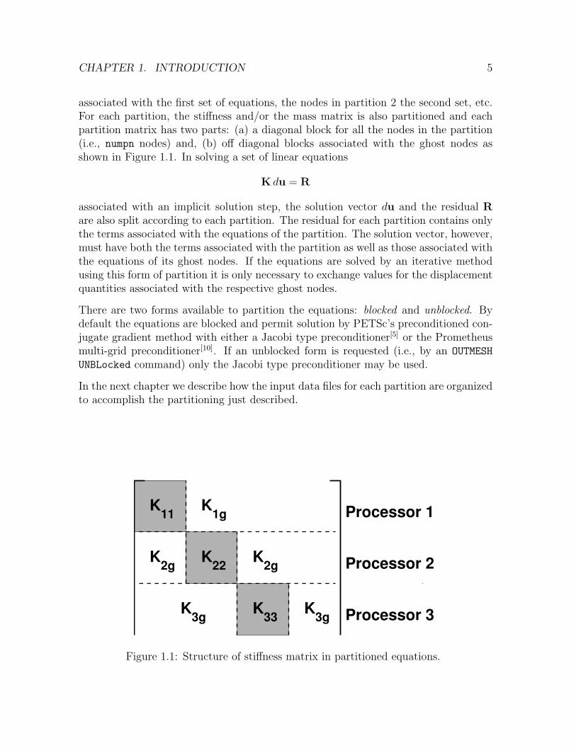
It is assumed that numd represents the number of processors to be used in the parallelsolution. Each partition is assigned numpn nodes. The number can differ slightly amongthe various partitions but is approximately the total number of nodes in the problemdivided by numd. In the current release, no weights are assigned to the nodes to reflectpossible diffences in solution effort. It is next necessary to check which elements areattached to each of these nodes. Once this is performed it is then necessary to checkeach of the attached elements for any additional nodes that are not part of the currentnodal partition. These are called ghost nodes. The sum of the nodes in a partition(numpn) and its ghost nodes defines the total number of nodes in the current partitiondata file (i.e., the total number of nodes, numnp, in each mesh partition).
In the parallel solution the global equations are numbered sequentially from 1 to thetotal number of equations in the problem (numteq). The nodes in partition 1 are
1Use of this command set requires the path to the location of the partition program to be set inthe pstart.F file located in the parfeap directory.
CHAPTER 1. INTRODUCTION 5
associated with the first set of equations, the nodes in partition 2 the second set, etc.For each partition, the stiffness and/or the mass matrix is also partitioned and eachpartition matrix has two parts: (a) a diagonal block for all the nodes in the partition(i.e., numpn nodes) and, (b) off diagonal blocks associated with the ghost nodes asshown in Figure 1.1. In solving a set of linear equations
K du = R
associated with an implicit solution step, the solution vector du and the residual Rare also split according to each partition. The residual for each partition contains onlythe terms associated with the equations of the partition. The solution vector, however,must have both the terms associated with the partition as well as those associated withthe equations of its ghost nodes. If the equations are solved by an iterative methodusing this form of partition it is only necessary to exchange values for the displacementquantities associated with the respective ghost nodes.
There are two forms available to partition the equations: blocked and unblocked. Bydefault the equations are blocked and permit solution by PETSc’s preconditioned con-jugate gradient method with either a Jacobi type preconditioner[5] or the Prometheusmulti-grid preconditioner[10]. If an unblocked form is requested (i.e., by an OUTMESH
UNBLocked command) only the Jacobi type preconditioner may be used.
In the next chapter we describe how the input data files for each partition are organizedto accomplish the partitioning just described.
K11 K1g Processor 1
K2g K22 K2g Processor 2
K33K3g K3g Processor 3
Figure 1.1: Structure of stiffness matrix in partitioned equations.
Chapter 2
Input files for parallel solution
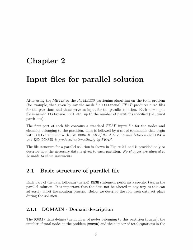
After using the METIS or the ParMETIS partioning algorithm on the total problem(for example, that given by say the mesh file Ifilename) FEAP produces numd filesfor the partitions and these serve as input for the parallel solution. Each new inputfile is named Ifilename 0001, etc. up to the number of partitions specified (i.e., numdpartitions).
The first part of each file contains a standard FEAP input file for the nodes andelements belonging to the partition. This is followed by a set of commands that beginwith DOMAin and end with END DOMAIN. All of the data contained between the DOMAin
and END DOMAIN is produced automatically by FEAP.
The file structure for a parallel solution is shown in Figure 2.1 and is provided only todescribe how the necessary data is given to each partition. No changes are allowed tobe made to these statements.
2.1 Basic structure of parallel file
Each part of the data following the END MESH statement performs a specific task in theparallel solution. It is important that the data not be altered in any way as this canadversely affect the solution process. Below we describe the role each data set playsduring the solution.
2.1.1 DOMAIN - Domain description
The DOMAIN data defines the number of nodes belonging to this partition (numpn), thenumber of total nodes in the problem (numtn) and the number of total equations in the
6

CHAPTER 2. INPUT FILES FOR PARALLEL SOLUTION 7
FEAP * * Start record and title...
Control and mesh description data for a partition...
END MESH
DOMAinnumpn numtn numteq
<BLOCked> equations: Block size = ndf
LOCAl to GLOBal node numbers...
GETData POINter nget_pnt...
GETData VALUes nget_val...
SENDdata POINter nsend_pnt...
SENDdata VALUes nsend_val...
MATRix storage...
<EQUAtion> numbers (If BLOCked not used)...
END DOMAIN
INCLude solve.filename
STOP
Figure 2.1: Input file structure for parallel solution.

CHAPTER 2. INPUT FILES FOR PARALLEL SOLUTION 8
problem (numteq). Note that the number of nodes in the partition (numpn) is alwaysless or equal to the number of nodes given on the control record (numnp) due to thepresence of the ghost nodes. The sum over all partitions of the number of nodes ineach partition (numpn) is equal to the total number of nodes in the problem (numtn).
2.1.2 BLOCked - Block size for equations
This data set is optional. If a blocked form for the equations is requested (this isthe default) this data set defines the block size. The block size is always equal to thenumber of degrees of freedom specified on the control record (i.e., ndf) and the blockedform of the equations is grouped into small blocks of size ndf.
2.1.3 LOCal to GLOBal node numbering
Each record in this set defines three values: (1) a local node number in the partition;(2) the global node associated with the local number; and (3) the global equation blocknumber associated with the local node. The first numpn records in the set are the nodesassociated with the current partition the remaining records with the ghost nodes.
2.1.4 GETData and SENDdata - Ghost node retrieve andsend
The current partition retrieves (GETData) the solution values for its ghost nodes fromother partitions. The data is divided into two parts: (1) A POINTER part which tellsthe number of values to obtain from each partition and (2) The VALUes list of localnode numbers needing values. The pointer data is given as
GETData POINter nparts
np_1
np_2
...
np_nparts
where np i defines the number in partition-i (note the number should be a zero for thecurrent partition record). The nodal values list is given as
GETData VALUes nvalue
local_node_1

CHAPTER 2. INPUT FILES FOR PARALLEL SOLUTION 9
local_node_2
...
local_node_nvalue
The local node i numbers are grouped so that the first np 1 are obtained from pro-cessor 1, the next np 2 from processor 2, etc. The local node 1 is the number of alocal ghost node to be obtained from another processor and may appear only once inthe list of GETData VALUes.
A corresponding pair of lists is given for the data to be sent (SENDdata) to the otherprocessors. The lists have identical structure to the GETData lists and are given by
SENDdata POINter nparts
np_1
np_2
...
np_nparts
and
SENDdata VALUes nvalue
local_node_1
local_node_2
...
local_node_nvalue
where again the local node i numbers are grouped so that the first np 1 are sent toprocessor 1, the next np 2 to processor 2, etc. It is possible for a local node numberto appear more than once in the SENDdata VALUes list as it could be a ghost node formore than one other partition.
2.1.5 MATRix storage – equation structure
Each equation in the global matrix consists of the number of terms that are associatedwith the current partition and the number of terms associated with other partitions.This information is provided for each equation (equation block) by the MATRix storage
data set. Each record in the set is given by the global equation number followed bythe number of terms associated with the current partition and then the number ofterms associated with other partitions. The use of this data is critical to obtain rapidassembly of the global matrices by PETSc. If it is incorrect the assembly time will bevery large compared to the time needed to compute the matrix coefficients.

CHAPTER 2. INPUT FILES FOR PARALLEL SOLUTION 10
When the equations are blocked the data is given for each block number. In the blockedform every node has ndf equations. Thus, the first ndf equations are associated withblock 1, the second with block 2, etc. The total number of equations numteq for thisform is numtn × ndf. Each record of the MATRix storage data is given by the globalblock number, the number of blocks associated with the current partition and thenumber of blocks associated with other partitions. For any node in which all degree-of-freedoms (DOF) are of displacement type the number of blocks in the current partitionwill be 1 and the number in other blocks will be zero. That is, the equations for anynode in which all DOF’s are fixed will be given as:
I dua = Ra = du
where du denotes a specified valued for the solution.
2.1.6 EQUAtion number data
This data set is not present when the equations are blocked. However, when the equa-tions are unblocked it is necessary to fully describe the equation numbering associatedwith each node in the partition. This is provided by the EQUAtion number data set.The set consists of numnp records which contain the local node number followed bythe global equation number for every degree-of-freedom associated with the node. If adegree-of-freedom is restrained (i.e., of displacement type) the equation is not activeand a zero appears. This form results in fewer unknown values but may not be usedwith any equation solution requiring a blocked form (in particular, Prometheus).
2.1.7 END DOMAIN record
The parallel data is terminated by the END DOMAIN record. It is followed by the solutioncommands.

Chapter 3
Solution process
Once the parallel input mesh files are created an execution of the parallel version offeap may be performed using the command line statement
-@$MPIRUN -s all -np $(NPROC) $(FEAPRUN) -ksp_type cg -pc_type jacobi
or
-@$MPIRUN -s all -np $(NPROC) $(FEAPRUN) -ksp_type cg -pc_type prometheus
(for details on other required and optional parameters see the makefile in the parfeapsubdirectory). The parameters setting the number of processors (NPROC) and the exe-cution path FEAPRUN must be defined before issuing the command.
Once FEAP starts the input file should be set to Ifilename 0001 where filename isthe name of the solution file to be solved. Each processor reads its input file up to theEND MESH statement and then starts processing command language statements.
In a parallel solution using FEAP the same command language statements must beprovided for each partition. This is accomplished using the statement
INCLude solve.filename
where filename is the name of the input data file with the leading I and the trailingpartition number removed. Thus for the file named Iblock 0001 the command is givenas solve.block. All solution commands are then placed in a file with this name andcan include both BATCh and INTEractive commands. For example a simple solutionmay be given by the commands
11

CHAPTER 3. SOLUTION PROCESS 12
BATCh
PETSc ON
TOL ITER 1.d-07 1.d-08 1.d+20
TANGent,,1
END
INTEractive
placed in the solve.filename file. Note hat both batch and interactive modes ofsolution are optionally included. Interactive commands need only be entered onceand are sent to other processors automatically if in the makefile for initiating theexecution of the parallel FEAP the target parameter -s all appears. In the subse-quent subse4ctions we describe some of the special commands that control the parallelexecution mode of FEAP
3.1 Command language statements
Most of the standard command language statements available in the serial version ofFEAP (see users manual [1]) may be used in the parallel version of feap. New com-mands are available also that are specifically related to performing a parallel solution.
3.1.1 PETSc Command
The PETSc command is used to activate the parallel solution process. The command
PETSc <ON,OFF>
may be used to turn on and off the parallel execution It is only required for singleprocessor solutions and is optional when two or more processors are used in the solutionprocess. When required, it should always be the first solution command.
The command may also be used with the VIEW parameter to create outputs for thetangent matrix, solution residual or mass matrix. Thus, use as
PETSc VIEW
MASS
PETSc NOVIew
will create a file named mass.m that contains all the non-zero values of the total massmatrix. The parameter VIEW turns on output arrays and this remains in effect for all

CHAPTER 3. SOLUTION PROCESS 13
commands until the command is given with the NOVIew parameter. The file is createdin a format that may be directly used by MATLAB.[11] This command should only beused with small problems to verify the correctness of results as large files will resultotherwise.
3.2 Solution of linear equations
The parallel version of FEAP can use all of the SLES (linear solvers) available in PETScas well as the parallel multigrid solver, Prometheus[10]. The actual type of linear solverused is specified in the makefile located in the parfeap directory (see, Sect. 3 above).Once the solution is initiated the solution of linear equations is performed whenever aTANG,,1 or SOLVe command is given.
The types of solvers and the associated preconditioners tested to date are described inTable 3.1.
Solver Preconditioner NotesCG JacobiCG Prometheus Generally requires fewest iterationsMINRES JacobiMINRES PrometheusGMRES JacobiGMRES PrometheusGMRES Block Jacobi Often gives indefinite factor.GMRES ASM(ILU)
Table 3.1: Linear solvers and preconditioners tested.
The solvers, together with the necessary options for preconditioning may be specifiedin the Makefile as parameters to the mpirun command. Two examples of possibleoptions are contained in the Makefile.
3.2.1 Tolerance for equation solution
The basic form of solution for linear equations is currently restricted to a preconditionedconjugate gradient (PCG) method. Two basic solution forms are defined in the makefilecontained in the parfeap subdirectory. The first (feaprun) uses the solver contained inthe PETSc library and the second is Prometheus (feaprun-mg) available from ColumbiaUniversity.[10] In general the performance of Prometheus is much better than the firstform.

CHAPTER 3. SOLUTION PROCESS 14
Termination tolerances for the solvers are given by either
TOL ITER rtol atol dtol
or
ITER TOL rtol atol dtol
where rtol is the tolerance for the preconditioned equations, atol the tolerance forthe original equations and dtol a value at which divergence is assumed. The defaultvalues are:
rtol = 1.d− 8 ; atol = 1.d− 16 and dtol = 1.d + 16
For many problems it is advisable to check that the actual solution is accurate sincetermination of the equation solution is performed based on the rtol value. A checkshould be performed using the command sequence
TANG,,1
LOOP,,1
FORM
SOLV
NEXT
since the TANG command has significant set up costs, especially for Prometheus. Indeed,for some problems more than one iteration is needed in the loop.
3.2.2 GLIST & GNODE: Output of results with global nodenumbers
In normal execution each partition creates its own output file (e.g., Ofilename 0001,etc.) with printed data given with the local node and element numbers of the proces-sor’s input data file. In some cases the global node numbers are known and it is desiredto identify which processor to which the node is associated. This may be accomplishedby including a GLISt command in the solution statements along with the list of globalnode numbers to be output. The option is restricted to 3 lists, each with a maximumof 100 nodes. The command sequence is given by:
BATCh
GLISt,,<1,2,3>

CHAPTER 3. SOLUTION PROCESS 15
END
list of global node numbers, 8 per record
! blank termination record
The list will be converted by each processor into the local node numbers to be outputusing the command
DISP LIST <1,2,3>
The command may also be used with VELOcity, ACCEleration, and STREss. Seemanual pages in the FEAP Users Manual.[1]
It is also possible to directly output the global node number associated with individuallocal node numbers using the command statement
DISP GNODe nstart nend ninc
where nstart and nend are global node numbers. This command form also may beused with VELOcity, ACCEleration, and STREss.
3.3 Eigenproblem solution for modal problems
The computation of the natural modes and frequencies of free vibration of an undampedlinear structural problem requires the solution of the general linear eigenproblem
KΦ = MΦΛ
In the above K and M are the stiffness and mass matrices, respectively, and Φ and Λare the normal modes and frequencies squared. Normally, the constraint
ΦTMΦ = I
is used to scale the eigenvectors. In this case one also obtains the relation
ΦTKΦ = Λ
3.3.1 Subspace method solutions
The subspace algorithm contained in FEAP has been extended to solve the aboveproblem in a parallel mode. The use of the subspace algorithm requires a linear solutionof the equations
Kx = y

CHAPTER 3. SOLUTION PROCESS 16
for each vector in the subspace and for each subspace iteration. The parallel subspacesolution is performed using the command set
TANGent
MASS <LUMPed,CONSistent>
PSUBspace <print> nmodes <nadded>
where textttnmodes is the desired number of modes, nadded is the number of extravectors used to accelerate the convergence (default if maximum of nmodes and 8) andprint produces a print of the subspace projections of K and M. The accuracy of thecomputed eigenvalues is the maximum of 1.d−12 and the value set by the TOL solutioncommand. The method may be used with either a lumped or a consistend mass matrix.
If it is desired to extract 10 eigenvectors with 8 added vectors and 20 iterations areneeded to converge to an acceptable error it is necessary to perform 360 solutions of thelinear equations. Thus, for large problems the method will be very time consuming.
3.3.2 Arnoldi/Lanczos method solutions
In order to reduce the computational effort the Arnoldi/Lanczos methods implementedin the ARPACK module available from Rice University[12] has been modified to workwith the parallel version of FEAP.
Two modes of the ARPACK solution methods are included in the program:
1. Mode 1: Solves the problem reformed as
M−1/2 KM−1/2 Ψ = ΨΛ
whereΦ = M−1/2 Ψ
This form is most efficient when the mass matrix is diagonal (lumped) and, thus,in the current release of parallel FEAP is implemented only for diagonal (lumped)mass forms. This mode form is specified by the solution command set
TANGent
MASS LUMPed
PARPack LUMPed nmodes <maxiters> <eigtol>
where nmodes is the number of desired modes. Optionally, maxiters is thenumber of iterations to perform (default is 300) and eigtol the solution toleranceon eigenvalues (default is the maximum of 1.d − 12 and the values set by thecommand TOL.

CHAPTER 3. SOLUTION PROCESS 17
2. Mode 3: Solves the general linear eigenproblem directly and requires solution ofthe linear problem
Kx = y
for each iteration. Fewer iterations are normally required than in the subspacemethod, however, the method is generally far less efficient than the Mode 1 formdescribed above. This form is given by the set of commands
TANGent
MASS <LUMPed,CONSistent>
PARPack <SYMMetric> nmodes <maxiters> <eigtol>
Use of the command MASS alone also will employ a consistent mass (or the massproduced by the quadrature specified).
3.4 Graphics output
During a solution the graphics commands may be given in a standard manner. However,each processor will open a graphics window and display only the parts that belong tothat processor. Scaling is also done processor by processor unless the PLOT RANGe
command is used to set the range of a set of plot values.
3.4.1 GPLOt command
An option does exist to collect all the results together and present on a single graphicswindow. This option also permits postscript outputs to be constructed and saved infiles. To collect the results together it is necessary to write the results to disk for eachitem to be graphically presented. This is accomplished using the GPLOt command.This command has the options
GPLOt DISPlacement n
GPLOt STREss n
GPLOt PSTRess n
where n denotes the component of a displacement (DISP), nodal stress (STRE) or prin-cipal stress (PSTRE). Each use of the command creates a file on each processor with theform
Gproblem_domain.xyyyy

CHAPTER 3. SOLUTION PROCESS 18
where problem domain is the name of the problem file for the domain; x is d, s or pfor a displacement, stress or principal stress, respectively; and yyyy is a unique plotnumber (it will be between 0001 and 9999).
3.4.2 NDATa command
Once the GPLOt files have been created they may be plotted using a serial execution ofthe parallel FEAP program (i.e., using the Iproblem file. The command may be givenin INTEractive mode only as one of the options:
Plot > NDATa DISPl n
Plot > NDATa STREss n
Plot > NDATa PSTRess n
where n is the value of yyyy used to write the file.
WARNING: Plots by FEAP use substantial memory and thus this option may notwork for very large problems. One should minimize the number of commands usedduring input of the problem description (i.e., remove input commands in the meshthat create new memory).

Bibliography
[1] R.L. Taylor. FEAP - A Finite Element Analysis Program, User Manual. Univer-sity of California, Berkeley. http://www.ce.berkeley.edu/˜rlt.
[2] O.C. Zienkiewicz, R.L. Taylor, and J.Z. Zhu. The Finite Element Method: ItsBasis and Fundamentals. Butterworth-Heinemann, Oxford, 6th edition, 2005.
[3] O.C. Zienkiewicz and R.L. Taylor. The Finite Element Method for Solid andStructural Mechanics. Butterworth-Heinemann, Oxford, 6th edition, 2005.
[4] O.C. Zienkiewicz, R.L. Taylor, and P. Nithiarasu. The Finite Element Method forFluid Dynamics. Butterworth-Heinemann, Oxford, 6th edition, 2005.
[5] S. Balay, K. Buschelman, W.D. Gropp, D. Kaushik, M.G. Knepley,L.C. McInnes, B.F. Smith, and H. Zhang. PETSc Web page, 2001.http://www.mcs.anl.gov/petsc.
[6] S. Balay, K. Buschelman, V. Eijkhout, W.D. Gropp, D. Kaushik, M.G. Knepley,L.C. McInnes, B.F. Smith, and H. Zhang. PETSc users manual. Technical ReportANL-95/11 - Revision 2.1.5, Argonne National Laboratory, 2004.
[7] G. Karypis. METIS: Family of multilevel partitiong algorithms. http://www-users.ce.umn.edu/˜karypis/metis/.
[8] G. Karypis. ParMETIS parallel graph partitioning, 2003. http://www-users.cs.unm.edu/˜karypis/metis/parmetis/).
[9] S. Balay, W.D. Gropp, L.C. McInnes, and B.F. Smith. Efficient managementof parallelism in object oriented numerical software libraries. In E. Arge, A. M.Bruaset, and H. P. Langtangen, editors, Modern Software Tools in Scientific Com-puting, pages 163–202. Birkhauser Press, 1997.
[10] M. Adams. PROMETHEUS: Parallel multigrid solver library for unstructuredfinite element problems. http://www.columbia.edu/˜ma2325.
[11] MATLAB. www.mathworks.com, 2003.
19

BIBLIOGRAPHY 20
[12] R. Lehoucq, K. Maschhoff, D. Sorensen, and C. Yang. ARPACK: Arnoldi/lanczospackage for eigensolutions. http://www.caam.rice.edu/software/ARPACK/.
[13] R.L. Taylor. FEAP - A Finite Element Analysis Program, Installation Manual.University of California, Berkeley. http://www.ce.berkeley.edu/˜rlt.

Appendix A
Solution Command Manual Pages
FEAP has a few options that are used only to solve parallel problems. The comandsare additions to the command language approach in which users write each step usingavailable commands. The following pages summarize the commands currently addedto the parallel version of FEAP.
21

APPENDIX A. SOLUTION COMMAND MANUAL 22
DISPlacements FEAP COMMAND INPUT COMMAND MANUAL
disp,gnod,<n1,n2,n3>
Other options of this command are described in the FEAP User Manual. The com-mand DISPlacement may be used to print the current values of the solution generalizeddisplacement vector associated with the global node numbers of the original mesh. Thecommand is given as
disp,gnod,n1,n2,n3
prints out the current solution vector for global nodes n1 to n2 at increments of n3(default increment = 1). If n2 is not specified only the value of node n1 is output. Ifboth n1 and n2 are not specified only the first node solution is reported.

APPENDIX A. SOLUTION COMMAND MANUAL 23
GLISt FEAP COMMAND INPUT COMMAND MANUAL
glist,,n1
<values>
The command GLISt is used to specify lists of global node numbers for output ofnodal values. It is possible to specify up to three different lists where the list numbercorresponds to n1 (default = 1). The list of nodes to be output is input with up to8 values per record. The input terminates when less than 8 values are specified or ablank record is encountered. No more than 100 items may be placed in any one list.
List outputs are then obtained by specifying the command:
name,list,n1
where name may be DISPlacement,VELOcity,ACCEleration, or STREss and n1 is the desiredlist number.
Example:
BATCh
GLISt,,1
END
1,5,8,20
BATCh
DISP,LIST,1
...
END
The global list of nodes is processed to determine the processor and the associatedlocal node number. Each processor then outputs its active values (if any) and givesboth the local node number in the partition as well as the global node number.

APPENDIX A. SOLUTION COMMAND MANUAL 24
GPLOt FEAP COMMAND INPUT COMMAND MANUAL
gplo disp n
gplo velo n
gplo acce n
gplo stre n
Use of plot commands during execution of the parallel version of FEAP create the samenumber of graphic windows as processors used to solve the problem. Each windowcontains only the part of the problem contained on that processor.
The use of the GPLOt command is used to save files containing the results for all nodaldispacements, velocities, accelerations or stresses in the total problem. The only actionoccuring after the use of this command is the creation of a file containing the currentresults for the quantity specified. Repeated use of the command creates files withdifferent names.
These results may be processed by a single processor run of the problem using themesh for the total problem. To display the nodal values command NDATa is used. Seemanual page on NDATa.

APPENDIX A. SOLUTION COMMAND MANUAL 25
GRAPh FEAP COMMAND INPUT COMMAND MANUAL
grap,,num d
grap node num d
grap file
grap part num d
The use of the GRAPh command activates the interface to the METIS multilevel par-tioner. The partition into num d parts is performed based on a nodal graph. The nodalpartition divides the total number of nodes (i.e., numnp values) into num d nearly equalparts.
If the GRAPh command is given with the option file the partition data is input from thefile graph.filename where filename is the same as the input file without the leadingI character. The data contained in the graph.filename is created using the standalone partitioner program which employs the PARMETIS multilevel partitioner.
It is also possible to execute PARMETIS to perform the partitioning directly duringa mesh input. It is necessary to have a mesh which contains all the nodal coordinateand element data in the input file. This is accomplished using the command set
OUTMesh
GRAPh PARTition num_d
OUTDomain meshes
where num d is the number of domains to create. The command OUTMesh creates afile with all the nodal and element data and is destroyed after execution of the GRAPh
command.

APPENDIX A. SOLUTION COMMAND MANUAL 26
ITERative FEAP COMMAND INPUT COMMAND MANUAL
iter,,,icgit
iter,bpcg,v1,icgit
iter,ppcg,v1,icgit
iter,tol,v1,v2,v3
The ITERative command sets the mode of solution to iterative for the linear algebraicequations generated by a TANGent. Currently, iterative options exist only for symmetric,positive definite tangent arrays, consequently the use of the UTANgent command shouldbe avoided. An iterative solution requires the sparse matrix form of the tangent matrixto fit within the available memory of the computer.
Serial solutions
In the serial version the solution of the equations is governed by the relative residual forthe problem (i.e., the ratio of the current residual to the first iteration in the currenttime step). The tolerance for convergence may be set using the ITER,TOL,v1,v2 option.The parameter v1 controls the relative residual error given by
(RTR)1/2i ≤ v1 (RTR)
1/20
and, for implementations using PETSc the parameter v2 controls the absolute residualerror given by
(RTR)1/2i ≤ v2
The default for v1 is 1.0d-08 and for v2 is 1.0d-16. By default the maximum numberof iterations allowed is equal to the number of equations to be solved, however, thismay be reduced or increased by specifying a positive value of the paramter icgit.
The symmetric equations are solved by a preconditioned conjugate gradient method.Without options, the preconditioner is taken as the diagonal of the tangent matrix.Options exist to use the diagonal nodal blocks (i.e., the ndf × ndf nodal blocks, orreduced size blocks if displacement boundary conditions are imposed) as the precondi-tioner. This option is used if the command is given as ITERative,BPCG. Another optionis to use a banded preconditioner where the non-zero profile inside a specified half bandis used. This option is used if the command is given as ITERative,PPCG,v1, where v1 isthe size of the half band to use for the preconditioner.
The iterative solution options currently available are not very effective for poorly con-ditioned problems. Poor conditioning occurs when the material model is highly non-

APPENDIX A. SOLUTION COMMAND MANUAL 27
linear (e.g., plasticity); the model has a long thin structure (like a beam); or whenstructural elements such as frame, plate, or shell elements are employed. For compactthree dimensional bodies with linear elastic material behavior the iterative solution isoften very effective.
Another option is to solve the equations using a direct method (see, the DIREct com-mand language manual page).
Parallel solutions
For the parallel version the control of the PETSc preconditioned iterative solvers iscontrolled by the command
ITER TOL itol atol dtol
where itol is the tolerance for the preconditioned equations (default 1.d − 08), atolis the tolerance for the original equations (default 1.d − 16) and dtol is a divergenceprotection when the equations do not converge (default 1.d + 16).

APPENDIX A. SOLUTION COMMAND MANUAL 28
NDATa FEAP COMMAND INPUT COMMAND MANUAL
ndat disp n
ndat velo n
ndat acce n
ndat stre n
This command is used in a single processor execution using the mesh for the totalproblem. It is necessary for files to be created during a parallel execution using theGPLOt command (See manual page on GPLOt).
The command is given by
NDATa DISPlacement num
where the parameter num is the number corresponding to the order the DISPlacement
are created. Thus, the command sequence
NDATa DISPlacement 2
NDATa STREss 2
would display the results for the second files created for the displacements and stresses.

APPENDIX A. SOLUTION COMMAND MANUAL 29
OUTDomain FEAP COMMAND INPUT COMMAND MANUAL
outd,,<bsize>
outd bloc <bsize>
outd unbl
The use of the OUTDomain command may only be used after the GRAPh commandpartitions the mesh into num d parts (see GRAPh command language page for details).
Using the command OUTDomain or OUTDomain BLOCked creates num d input files for asubsequent parallel solution in which the coefficient arrays will be created in a blockedform. The parameter bsize defines the block size and must be an integer divisor ofndf. That is if ndf = 6 then bsize may be 1, 2, 3, or 6. By default each block inthe equations has a size ndf. The setting of the block size can significantly reduce theamount of storage needed to store the sparse coefficient matrix created by TANGent orUTANgent when a problem has a mix of element types. For example if a problem hasa large number of solid elements with 3 degrees of freedom per node and additionalframe or shell elements with 6 degrees of freedom per node, specifying bsize = 3 cansave considerable memory.

APPENDIX A. SOLUTION COMMAND MANUAL 30
PETSc FEAP COMMAND INPUT COMMAND MANUAL
pets
pets on
pets off
pets view
pets noview
The use of the PETSc command turns on or off to activate or deactivate parallelsolution options, respectively. To turn on parallel computing the command may begiven in the simple form: PETSc. When more than one partition is created, i.e., thenumber of solution processors is 2 or more, the PETSc option is on by default. Thecommand must be the first command of the command language program when only 1processor is used.
The option PETSc VIEW will result in a file for all the non-zero coefficients in the tangentmatrix to be output into a file. The output is in a MATLAB format. This option shouldonly be used for very small problems to check that a formulation produces correctresults (i.e., there is another set of terms to which a comparison is to be made). Theoption is turned off using the statement PETSc NOVIew. The default is NOVIew.

APPENDIX A. SOLUTION COMMAND MANUAL 31
STREss FEAP COMMAND INPUT COMMAND MANUAL
stre.gnod,<n1,n2,n3>
Other options for this command are given in the FEAP User Manual. The STREsscommand is used to output nodal stress results at global node numbers n1 to n2 atincrements of n2 (default = 1).
The command specified as:
stre,gnode,n1,n2,n3
If n3 is not given an increment of 1 is used. If n2 is not given only values for node n1
are output. If n1 is not specified the values at global node 1 are output.

APPENDIX A. SOLUTION COMMAND MANUAL 32
TOLerance FEAP COMMAND INPUT COMMAND MANUAL
tol,,v1
tol,ener,v1
tol,emax,v1
tol,iter,v1,v2,v3
The TOL command is used to specify the solution tolerance values to be used at variousstages in the analysis. Uses include:
1. Convergence of nonlinear problems in terms of the norm of energy in the currentiterate (the inner, dot, product of the displacement increment and the solutionresidual vectors).
2. Convergence of iterative solution of linear equations.
3. Convergence of the subspace eigenpair solution which is measured in terms of thechange in subsequent eigenvalues computed.
The basic command, TOL,,tol, without any arguments sets the parameter tol used inthe solution of non-linear problems where the command sequence
LOOP,,30
TANG,,1
NEXT
is given. In this case, the loop is terminated either when the number of iterationsreaches 30 (or whatever number is given in this position) or when the energy error isless than tol. The energy error is given by
Ei = (duTR)i ≤ tol (duTR)0 = E0
in which R is the residual of the equatons and du is the solution increment. The defaultvalue of tol for the solution of nonlinear problems is 1.0d-16.
The TOL command also permits setting a value for the energy below which convergenceis assumed to occur. The command is issued as TOL,ENERgy,v1 where v1 is the value ofthe converged energy (i.e., it is equivalent to the tolerance times the maximum energyvalue). Normally, FEAP performs nonlinear iterations until the value of the energyis less than the TOLerance value times the value of the energy from the first iteration

APPENDIX A. SOLUTION COMMAND MANUAL 33
as shown above. However, for some transient problems the value of the initial energyis approaching zero (e.g., for highly damped solutions which are converging to somesteady state limit). In this case, it is useful to specify the energy for convergencerelative to early time steps in the solution. Convergence will be assumed if either thenormal convergence criteria or the one relative to the specified maximum energy issatisfied.
The TOL command also permits setting the maximum energy value used for conver-gence. The command is issued as
TOL,EMAXimum,v1
where v1 is the value of the maximum energy quantity. Note that the TIME commandsets the maximum energy to zero, thus, the value of EMAXimum must be reset aftereach time step using, for example, a set of commands:
LOOP,time,n
TIME
TOL,EMAX,5.e+3
LOOP,newton,m
TANG,,1
NEXT
etc.
NEXT
to force convergence check against a specified maximum energy. The above two formsfor setting the convergence are nearly equivalent; however, the ENERgy tolerance formcan be set once whereas the EMAXimum form must be reset after each time command.
The command
TOL ITERation itol atol dtol
is used to control the solution accuracy when an iterative solution process is used tosolve the equations
K du = R
In this case the parameter itol sets the relative error for the solution accuracy, i.e.,when
(RTR)1/2i ≤ itol (RTR)
1/20
The parameter atol is only used when solutions are performed using the KSP schemesin a PETSc implementation to control the absolute residual error
(RTR)1/2i ≤ atol

APPENDIX A. SOLUTION COMMAND MANUAL 34
The dtol parameter is used to terminate the solution when divergence occurs. Thedefault for itol is 1.0d-08, that for atol is 1.0d-16 and for dtol is 1.0d+16.

Appendix B
Program structure
B.1 Introduction
This section describes the parallel infrastructure for the general purpose finite elementprogram, FEAP.[1] The current version of the parallel code modifies the serial versionof FEAP to interface to the PETSc library system available from Argonne NationalLaboriatories.[5, 6] In additioon the METIS[7] and ParMETIS[8] librairies are used topartion each mesh for parallel solution.
The necessary modifications and additions for the parallel features are contained in thedirectory parfeap. There are five sub-directories contained in parfeap:
1. arpack: Contains the subprograms and include files needed for the ARPACKeigen solution module (see Section 3.3).
2. blas: Contains Fortran versions of the BLAS routines used by FEAP. It isrecommended that when ever possible a BLAS library be used. These routinesare provided only for cases where no library is available.
3. lapack: Contains the subprograms from LAPACK used in the parallel version.
4. partition: Containts the progream and include file used to construct the parti-tion graph using ParMETIS (see Section 1.3).
5. windows: Contains the replacement for subprogram p metis.f for use in a Win-dows version of the program.1
1N.B. No testing of any parallel solutions other than mesh partitioning using a serial version ofFEAP has been attempted to date.
35

APPENDIX B. PROGRAM STRUCTURE 36
B.2 Building the parallel version
In order to build a parallel version of FEAP it is necessary first to install and compilea serival version (see instructions in the FEAP Installation manual.[13]). Once a serialversion is available and tested the routines in the arpack shoule be compiled using thecommand
make
while in the arpack subdirectory. This will build an archive named arpacklib.a.
The parallel version of FEAP is then compiled by executing the command
make feap
from the parfeap directory. If any subprogram are missing it may be necessary tocompile the programs in the lapack and/or blas subdirectories, modify the Makefile
in the parfeap directory and then recompile the program using the above command.If any errors still exist it is necessary to ensure that all definitions contained in theMakefile have been properly set using setenv and/or that PETSc has been properlyinstalled.

Appendix C
Element modification features
The use of the eigensolver with the LUMPed option requires all elements to form a validdiagonal (lumped) mass matrix. One option to obtain a lumped mass is the use of aquadrature formula that samples only at nodes.[2] In this case all element that use C0
interpolation forms have mass coefficients computed from
Mab =
∫Ωe
Na ρ Nb dV ≈∑
l
Na(ξl) ρ Nb(ξl) j(ξl) Wl
where ξl and Wl are the quadrature points and j(ξl) the jacobian of the coordinatetransformation. For C0 interpolations the shape frunctions have the property[2]
Na(ξb) = δab =
1 ; a = b0 ; a 6= b
Thus if ξl = ξb (the nodal points) and Wl > 0 the mass matrix produced will bediagonal and positive definite.
For quadrilateral and brick elements of linear order use of product forms of trapezoidalrule sample at all nodes ande satisfy the above criterion. Similarly use of Simpson’srule for quadratic order quadrilaterals or bricks also satisfies the above rule. Similarly,for triangular and tetrahedral elements of linear order nodal integrations has positiveweights and produces a valid diagonal mass. However, for a 6-node quadratic ordertriangle or a 10-node quadratic order tetrahedron no such formula exists. Indeed, thenodal quadrature formula for these elements samples only at the mid-edge nodes andhas zero weights Wb at the vertex nodes. Such a formula is clearly not valid for usein computing a diagonal mass matrix. The problem can be cured however by merelyadding an addition node at the baricenter of the triangle or tetrahedron and thusproducint a 7-node or 11-node element, respectively. Another advantage exists in thatthese elements may also be developed as mixed models that permit solution of problemsin which the material behavior is nearly incompressible (e.g., see references [2] and [3]).
37

APPENDIX C. ELEMENT MODIFICATION FEATURES 38
FEAP has been modified to include use of 7-node triangular and 11-node tetrahe-dral elements. Furthermore, nodal quadrature formulas have been added and may beactivated for each material by including the quadrature descriptor
QUADrature NODAl
or, alsternatively, for the whole problem as
GLOBal
QUADrature NODAl
! Other global options or blank record to terminate
Existing meshes of 10-node tetrahedral elements may be converted using the user func-tion umacr0.f included in the subdirectory parfeap. A similar function to convert6-node triangular element may be easily added using this function as a model.
The solution of problems composed of quadratic order tetrahedral elements can bedifficulty when elements have very bad aspect ratios or have large departures fromstraight edges. A more efficient solution is usually possible using linear order elements.Two options are available to convert 10-node tetrahedral elements to 4-node tetrahedralones. These are available as user functions in subdirectory parfeap. The first optionconverts each 10-node element to a single 4-node element. This leads to a problem withmany fewer nodes and, thus, is generally quite easy to solve compared to the originalproblem. This option is given in subprogram umacr8.f. A second option keeps thesame number of nodes and divides each 10-node element into eight (8) 4-node elements.This option is given in subprogram umacr9.f.
One final option exists o modify meshes with 10-node elements. In this option allcurved sides are made straight and mid-edge nodes are placed at the center of eachedge. This option is given in subprogram umacr6.f.

Appendix D
Added subprograms
The tables below describe the modifications and extensions to create the current parallelversion. Table D.1 describe modifications made to subroutines contained in the serialversion. Table D.2 presents the list of subprograms added to create the mesh for eachindividual processor and to permit basic parallel solution steps. Table D.3 presents thelist of subprograms modified for subspace eigensolution and those added to interfaceto the ARPACK Arnoldi/Lanczos eigensolution methods. Finally, Table D.4 describesthe list of user functions that may be introduced to permit various additional solutionsteps with the parallel or serial version.
39

APPENDIX D. ADDED SUBPROGRAMS 40
Filename Description of actions performed
filnam.F Set up file names for input/outputfppsop.F Output postscript file from each processorgamma1.f Compute energy for line searchpalloc.f Allocate memory for arrayspbases.F Parallel application of multiple base excitations for modal solutionspcontr.f Main driver for FEAPpdelfl.f Delete all temporary files at end of executionpextnd.f Dummy subprogram for external node determinationpform.f Parallel driver to compute element arrays and assemble global arrays
plstop.F Closes open plot windows, deletes arrays and stops executionpmacio.F Controls input of solution commandspmacr.f Solution command driver: Adds call to pmacr7 for parallel options
pmacr1.f Solution command driver 1pmacr3.f Solution command driver 3pmodal.f Parallel modal solution of linear transient problemspmodin.F Input initial conditions for jmodal solutionspplotf.F Driver for plot commandspremas.f Initalize data for mass computationprtdis.f Output nodal displacement values for real solutions: Includes global
node numbers for parallel runsprtstr.f Output nodal stress values: Includes global node numbers for parallel
runspstart.F Set starting values and control names of data files for each processorscalev.F Parallel scale of vector to have maximum element of +1.0
Table D.1: Subprograms modified for parallel solutions.
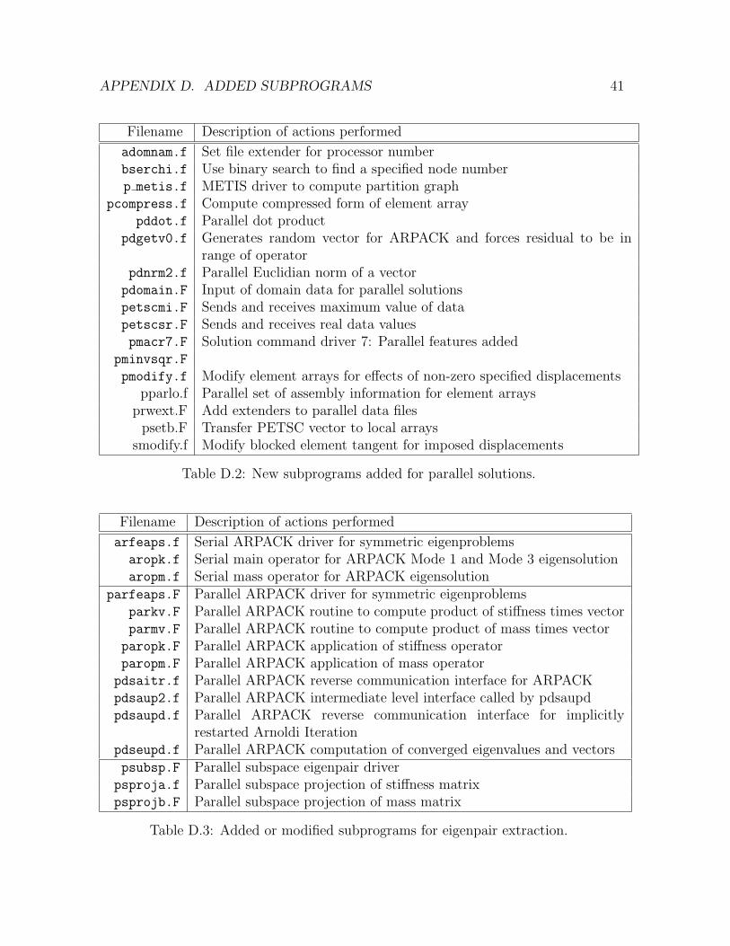
APPENDIX D. ADDED SUBPROGRAMS 41
Filename Description of actions performed
adomnam.f Set file extender for processor numberbserchi.f Use binary search to find a specified node numberp metis.f METIS driver to compute partition graph
pcompress.f Compute compressed form of element arraypddot.f Parallel dot product
pdgetv0.f Generates random vector for ARPACK and forces residual to be inrange of operator
pdnrm2.f Parallel Euclidian norm of a vectorpdomain.F Input of domain data for parallel solutionspetscmi.F Sends and receives maximum value of datapetscsr.F Sends and receives real data valuespmacr7.F Solution command driver 7: Parallel features added
pminvsqr.F
pmodify.f Modify element arrays for effects of non-zero specified displacementspparlo.f Parallel set of assembly information for element arrays
prwext.F Add extenders to parallel data filespsetb.F Transfer PETSC vector to local arrays
smodify.f Modify blocked element tangent for imposed displacements
Table D.2: New subprograms added for parallel solutions.
Filename Description of actions performed
arfeaps.f Serial ARPACK driver for symmetric eigenproblemsaropk.f Serial main operator for ARPACK Mode 1 and Mode 3 eigensolutionaropm.f Serial mass operator for ARPACK eigensolution
parfeaps.F Parallel ARPACK driver for symmetric eigenproblemsparkv.F Parallel ARPACK routine to compute product of stiffness times vectorparmv.F Parallel ARPACK routine to compute product of mass times vector
paropk.F Parallel ARPACK application of stiffness operatorparopm.F Parallel ARPACK application of mass operator
pdsaitr.f Parallel ARPACK reverse communication interface for ARPACKpdsaup2.f Parallel ARPACK intermediate level interface called by pdsaupdpdsaupd.f Parallel ARPACK reverse communication interface for implicitly
restarted Arnoldi Iterationpdseupd.f Parallel ARPACK computation of converged eigenvalues and vectorspsubsp.F Parallel subspace eigenpair driver
psproja.f Parallel subspace projection of stiffness matrixpsprojb.F Parallel subspace projection of mass matrix
Table D.3: Added or modified subprograms for eigenpair extraction.

APPENDIX D. ADDED SUBPROGRAMS 42
Filename Description of actions performed
uasble.F Parallel assembly of element stiffness arrays into PETSc matricesuasblem.F Parallel assembly of element mass arrays into PETSc matricesumacr4.f Parallel ARPACK interface for PETSc instructionsumacr5.f Serial ARPACK interface for PETSc instructionsumacr6.f Average coordinate locations for mid-edge nodes on quadratic order
elementsumacr7.f Convert 10-node tetrahedral elements into 11-node tetrahedraumacr8.f Convert mesh of 10-node tetrahedral elements into mesh of 4-node
tetrahedraumacr9.f Convert mesh of 10-node tetrahedral elements into mesh of 4-node
tetrahedral elementsumacr0.f Convert mesh of 10-node tetrahedral elements into mesh of 11-node
tetrahedral elementsupc.F Sets up user defined preconditioners (PC) for PETSc solutions
upremas.F Parallel interface to initialize mass assembly into PETSc arraysusolve.F Parallel solver interface for PETSc linear solutions
Table D.4: Modified and new user subprograms.
Appendix E
Parallel Validation
The validation of the parallel portion of FEAP has been performed on a number ofdifferent basic problems to verify that the parallel extension of FEAP will solve suchproblems and that the parallel version performs properly in the sense that it scaleswith processor number in an acceptable manner. Furthermore, a series of comparisontests have been performed to verify that the parallel version of the program producesthe same answers as the serial version. Because of the enormous variety of analysesthat one can perform with FEAP, it is not possible to provide parallel tests for allpossible combinations of program features. Nonetheless, below one will find somebasic validation tests that highlight the performance of the parallel version of the codeon a variety of problems.
All validation tests were performed on a cluster of AMD Opteron 250 processors,connected together via a Quadrics QsNet II interconnect. Code performance is oftenstrongly related to the computational sub-systems employed. All tests reported utilizedGCC v3.3.4, MPI v1.2.4, PETSc v2.3.2-p3, AMD ACML (BLAS/LAPACK) v3.5.0,ParMetis v3.1, Prometheus v1.8.5, and ARPACK c©2001. The batch scheduler assuresthat no other jobs are running on the same compute nodes during the runs. All runshave utilized the algebraic multigrid solver Prometheus in blocked form with coordinateinformation. Run times are as reported from PETSc summary statistics from a singlerun; Mflops are those associated with PETSc’s KSPsolve object; Number of solves isthe total number of Ax = b solves during the KSP iterations in the total problem, andScaling % of ideal is computed as (Mflopsnp/np)/(Mflops2/2)× 100.
43
APPENDIX E. PARALLEL VALIDATION 44
E.1 Timing Tests
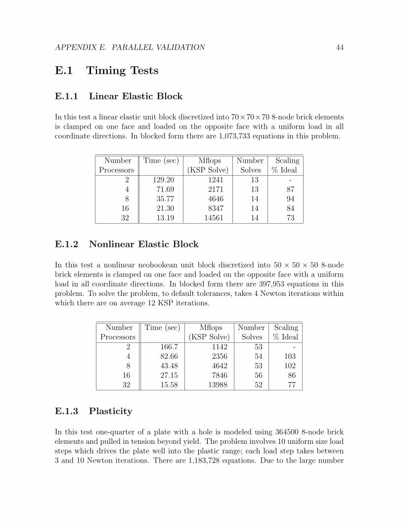
E.1.1 Linear Elastic Block
In this test a linear elastic unit block discretized into 70×70×70 8-node brick elementsis clamped on one face and loaded on the opposite face with a uniform load in allcoordinate directions. In blocked form there are 1,073,733 equations in this problem.
Number Time (sec) Mflops Number ScalingProcessors (KSP Solve) Solves % Ideal
2 129.20 1241 13 -4 71.69 2171 13 878 35.77 4646 14 94
16 21.30 8347 14 8432 13.19 14561 14 73
E.1.2 Nonlinear Elastic Block
In this test a nonlinear neohookean unit block discretized into 50 × 50 × 50 8-nodebrick elements is clamped on one face and loaded on the opposite face with a uniformload in all coordinate directions. In blocked form there are 397,953 equations in thisproblem. To solve the problem, to default tolerances, takes 4 Newton iterations withinwhich there are on average 12 KSP iterations.
Number Time (sec) Mflops Number ScalingProcessors (KSP Solve) Solves % Ideal
2 166.7 1142 53 -4 82.66 2356 54 1038 43.48 4642 53 102
16 27.15 7846 56 8632 15.58 13988 52 77
E.1.3 Plasticity
In this test one-quarter of a plate with a hole is modeled using 364500 8-node brickelements and pulled in tension beyond yield. The problem involves 10 uniform size loadsteps which drives the plate well into the plastic range; each load step takes between3 and 10 Newton iterations. There are 1,183,728 equations. Due to the large number

APPENDIX E. PARALLEL VALIDATION 45
of overall KSP iterations needed for this problem, it has only been solved using 8, 16,and 32 processors. Scaling is thus computed relative to the 8 processor run.
Number Time (sec) Mflops Number ScalingProcessors (KSP Solve) Solves % Ideal
2 - - - -4 - - - -8 220.80 4434 2973 -
16 107.70 8425 2908 9532 59.03 15645 2868 88
E.1.4 Box Beam: Shells
In this test a box beam is modeled using 40000 linear elastic 4-node shell elements (6-dof per node). The beam has a 1 to 1 aspect ratio with each face modeled by 100×100elements. One end is fully clamped and the other is loaded with equal forces in thethree coordinate directions. There are 242,400 equations; the block size is 6× 6.
Number Time (sec) Mflops Number ScalingProcessors (KSP Solve) Solves % Ideal
2 49.43 510 195 -4 16.37 1619 190 1598 12.46 1972 188 97
16 5.03 5246 181 12932 3.28 8177 184 100
E.1.5 Linear Elastic Block: 10-node Tets
In this test the linear elastic unit block from the first test is re-discretized using 10-nodetetrahedral elements. As in the 8-node brick case, there are 1,073,733 equations in thisproblem. In the table below, we also provide the ratio of times for the “same” prob-lem when solved using 8-node brick elements. This indicates the difficulty in solvingproblems (iteratively) that emanate from quadratic approximations. Essentially, perdof, tets solve in the ideal case 1.5 times slower.

APPENDIX E. PARALLEL VALIDATION 46
Number Time (sec) Mflops Number Scaling Slow downProcessors (KSP Solve) Solves % Ideal vs. Brick
2 216.8 1299 30 - 1.74 110.4 2615 30 101 1.58 56.62 5059 29 97 1.6
16 31.44 9370 30 90 1.532 17.07 17659 28 85 1.3
E.1.6 Transient
In this test a short (2 to 1 aspect ratio) neohookean beam is subjected to a stepdisplacement in the axial direction. The modeling employs symmetry boundary con-ditions on three orthogonal planes. The beam is discretized into uniform size 8-nodebrick elements 10 × 10 × 20 for a total of 7623 equations. The dynamic vibrations ofthe material are followed for 40 time steps using Newmark’s method. The steep dropoff in performance should be noted. This is due to the small problems size. There istoo little work for each processor to be effectively utilized here.
Number Time (sec) Mflops Number ScalingProcessors (KSP Solve) Solves % Ideal
2 95.37 1079 1385 -4 58.91 1687 1420 788 39.03 2645 1382 61
16 32.15 3138 1376 3632 33.61 3123 1371 18
E.1.7 Mock turbine
In this test we model a mock turbine fan blade with 12 fins. The system is loaded usingan Rω2 body force term which is computed consistently. Overall there are 1,080,0008-node brick elements in the mesh and 3,415,320 equations. It should be noted thatproblem, at roughly 3.5 million equations, provides enough work for the processors thateven at 32 processors there is no degradation of performance. The scaling is perfect.

APPENDIX E. PARALLEL VALIDATION 47
Number Time (sec) Mflops Number ScalingProcessors (KSP Solve) Solves % Ideal
2 854.3 806 116 -4 362.4 1931 112 1208 172.9 4085 110 127
16 88.99 8232 115 12832 46.68 16159 112 125
E.1.8 Mock turbine Small
In this test we model again a mock turbine fan blade with 12 fins. The system is loadedusing an Rω2 body force term which is computed consistently. Overall, however, thereare only 552960 8-node brick elements in the mesh and 1,771,488 equations.
Number Time (sec) Mflops Number ScalingProcessors (KSP Solve) Solves % Ideal
2 347.40 1097 125 -4 199.50 1878 132 868 91.63 4064 122 93
16 47.68 8024 126 9132 26.32 15400 119 88
E.1.9 Mock turbine Tets
In this test we model again a mock turbine fan blade with 12 fins. The system is loadedusing an Rω2 body force term which is computed consistently. This time however weutilize 10-node tetrahedral elements with a model that has 1,771,488 equations. Thiscomputation can be directly compared to the small mock turbine benchmark. Theslow down is given in the last column of the table below.
Number Time (sec) Mflops Number Scaling Slow DownProcessors (KSP Solve) Solves % Ideal vs. Brick
2 507.7 1193 126 - 1.54 304.2 1934 129 81 1.58 131.0 4675 131 98 1.4
16 70.01 8860 134 93 1.532 41.83 16238 127 85 1.6

APPENDIX E. PARALLEL VALIDATION 48
E.1.10 Eigenmodes of Mock Turbine
In this test we look at the computation of the first 5 eigen modes of the small (552960element) mock turbine model. Again, the mesh is composed of 8-node brick elementsand the model has 1,771,488 equations. A lumped mass is utilized and the algorithmtested is the ARPA symmetric option. Due to the large number of inner-outer iterationsthe timing runs are done only for 8, 16, and 32 processors. Scaling is thus computedrelative to the 8 processor run.
Number Time (sec) Mflops Number ScalingProcessors (KSP Solve) Solves % Ideal
2 - - - -4 - - - -8 916.9 3757 2744 -
16 507.1 7122 2876 9532 248.3 14042 2723 93
E.2 Serial to Parallel Verification
Serial to parallel code verification is reported upon below. For all test run, the programis run in serial mode (with a direct solver) and in parallel mode on 4 processors (forcinginter- and intra-node communications). Then various compuation output quantitiesare compared between the parallel and serial runs. In all cases, it is observed that theoutputs match to the computed accuracy.
E.2.1 Linear elastic block
In this test a linear elastic unit block discretized into 5× 5× 5 8-node brick elementsis clamped on one face and loaded on the opposite face with a uniform load in allcoordinate directions. The displacements are compared at global nodes 100 and 200and the maximum overall principal stress is also determined from both runs. All valuesare seen to be identical. For the parallel runs, the processor number containing thevalue is given in parenthesis and the reported node number is the local processor nodenumber.
Serial DisplacementsNode x-coor y-coor z-coor x-disp y-disp z-disp
100 6.00E-01 8.00E-01 4.00E-01 -1.3778E-01 1.1198E+00 1.1241E+00200 2.00E-01 6.00E-01 1.00E+00 -4.1519E-01 2.3568E-01 2.6592E-01

APPENDIX E. PARALLEL VALIDATION 49
Serial Max Principal StressNode Stress
1 4.0881E+02
Parallel Displacements(P)Node x-coor y-coor z-coor x-disp y-disp z-disp
(4)49 6.00E-01 8.00E-01 4.00E-01 -1.3778E-01 1.1198E+00 1.1241E+00(2)38 2.00E-01 6.00E-01 1.00E+00 -4.1519E-01 2.3568E-01 2.6592E-01
Parallel Max Principal Stress(P)Node Stress
(3)1 4.0881E+02
Note: Processor 3’s local node 1 corresponds to global node 1.
E.2.2 Box Beam
In this test a linear elastic unit box-beam discretized into 4 × 20 × 20 4-node shellelements is clamped on one face and loaded on the opposite face with a uniform loadin all coordinate directions. The displacements are compared at global nodes 500 and1000 and the maximum overall principal bending moment is also determined from bothruns. All values are seen to be identical. For the parallel runs, the processor numbercontaining the value is given in parenthesis and the reported node number is the localprocessor node number.
Serial Displacements/RotationsNode x-coor y-coor z-coor x-disp y-disp z-disp
x-rot y-rot z-rot500 8.00E-01 1.00E-01 1.00E+00 3.6632E-03 -3.2924E-03 2.3266E-03
4.4272E-02 -7.3033E-04 -2.1595E-021000 1.00E+00 3.00E-01 2.00E-01 2.2972E-02 1.5303E-03 1.6876E-02
4.8140E-02 2.8224E-02 -1.3278E-01
Serial Max PrincipalBending Moment
Node Stress1 1.7091E+01

APPENDIX E. PARALLEL VALIDATION 50
Parallel Displacements/Rotations(P)Node x-coor y-coor z-coor x-disp y-disp z-disp
x-rot y-rot z-rot(1)29 8.00E-01 1.00E-01 1.00E+00 3.6632E-03 -3.2924E-03 2.3266E-03
4.4272E-02 -7.3033E-04 -2.1595E-02(2)280 1.00E+00 3.00E-01 2.00E-01 2.2972E-02 1.5303E-03 1.6876E-02
4.8140E-02 2.8224E-02 -1.3278E-01
Parallel Max PrincipalBending Moment
(P)Node Stress(4)1 1.7091E+01
Note: Processor 4’s local node 1 corresponds to global node 1.
E.2.3 Linear Elastic Block: Tets
In this test a linear elastic unit block discretized into 162 10-node tetrahedral elementsis clamped on one face and loaded on the opposite face with a uniform load in allcoordinate directions. The displacements are compared at global nodes 55 and 160and the maximum overall principal stress is also determined from both runs. Allvalues are seen to be identical. For the parallel runs, the processor number containingthe value is given in parenthesis and the reported node number is the local processornode number.
Serial DisplacementsNode x-coor y-coor z-coor x-disp y-disp z-disp
55 8.33E-01 0.00E+00 1.67E-01 4.9509E-01 4.3175E-01 4.2867E-01160 8.33E-01 1.67E-01 5.00E-01 2.1305E-01 4.2030E-01 4.1548E-01
Serial MaxPrincipal Stress
Node Stress8 9.0048E+01
Parallel Displacements(P)Node x-coor y-coor z-coor x-disp y-disp z-disp
(3)23 8.33E-01 0.00E+00 1.67E-01 4.9509E-01 4.3175E-01 4.2867E-01(1)17 8.33E-01 1.67E-01 5.00E-01 2.1305E-01 4.2030E-01 4.1548E-01

APPENDIX E. PARALLEL VALIDATION 51
Parallel MaxPrincipal Stress
(P)Node Stress(4)6 9.0048E+01
Note: Processor 4’s local node 6 corresponds to global node 8.
E.2.4 Mock Turbine: Modal Analysis
In this test we examine a small mock turbine model with 30528 equations, where thediscretization is made with 8-node brick elements. We compute using the serial code(subspace method) the first 5 eigenvalues using a lumped mass. With the parallelcode, we compute the same eigenvalues using a parallel eigensolve (implicitly restartedArnoldi). The computed frequencies and from the first 5 modes are compared and seento be the same within the accuracy of the computation.
Serial Eigenvalues (rad/sec)2
Mode 1 Mode 2 Mode 3 Mode 4 Mode 58.10609997E-02 8.13523152E-02 8.13523152E-02 9.33393875E-02 9.33393875E-02
Parallel Eigenvalues (rad/sec)2
8.10609790E-02 8.13522933E-02 8.13522972E-02 9.33393392E-02 9.33393864E-02
The comparison of eigenvectors is a bit harder for this problem because of repeatedeigenvalues. The first eigenvalue is not repeated and it can easily be seen that the se-rial and parallel codes have produced the same eigenmode (up to an arbitrary scalingfactor). Eigenvalues 2 and 3 are repeated and thus the vectors computed are, permis-sibly, drawn from a subspace and thus direct comparison is not evident. The sameholds for eigenvalues 4 and 5; though, it can be observed that vector 4 from the serialcomputation does closely resemble vector 5 from the parallel computations – i.e. theyappear to be drawn from a similar region of the subspace.
As a test of the claim of differing eigenmodes due to selection of different eigenvectorsfrom a subspace, we also compute the first 5 modes of an asymmetric structure thatdoes not possess repeated eigenvalues. The basic geometry is that of perturbed cube.The first 5 eigenvalues and modes are compared and show proper agreement to withinthe accuracy of the computations for both the eigenvalues and the eigenmodes.

APPENDIX E. PARALLEL VALIDATION 52
-6.02E-02-4.82E-02-3.61E-02-2.41E-02-1.20E-02 8.68E-14 1.20E-02 2.41E-02 3.61E-02 4.82E-02 6.02E-02
-7.23E-02
7.23E-02
_________________ DISPLACEMENT 1
Value = 4.53E-02 Hz.
-2.88E-04-2.30E-04-1.73E-04-1.15E-04-5.75E-05 9.00E-12 5.75E-05 1.15E-04 1.73E-04 2.30E-04 2.88E-04
-3.45E-04
3.45E-04
_________________ EIGENV 1
Time = 0.00E+00
Figure E.1: Comparison of Serial (left) to Parallel (right) mode shape 1 degree offreedom 1.
-5.89E-02-4.72E-02-3.54E-02-2.36E-02-1.18E-02-4.54E-05 1.17E-02 2.35E-02 3.53E-02 4.71E-02 5.88E-02
-7.07E-02
7.06E-02
_________________ DISPLACEMENT 2
Value = 4.54E-02 Hz.
-2.54E-04-2.03E-04-1.52E-04-1.01E-04-5.07E-05 6.36E-08 5.08E-05 1.02E-04 1.52E-04 2.03E-04 2.54E-04
-3.04E-04
3.04E-04
_________________ EIGENV 2
Time = 0.00E+00
Figure E.2: Comparison of Serial (left) to Parallel (right) mode shape 2 degree offreedom 2.
-8.33E-01-6.67E-01-5.00E-01-3.33E-01-1.67E-01 3.91E-10 1.67E-01 3.33E-01 5.00E-01 6.67E-01 8.33E-01
-1.00E+00
1.00E+00
_________________ DISPLACEMENT 3
Value = 4.54E-02 Hz.
-5.64E-03-4.51E-03-3.38E-03-2.26E-03-1.13E-03 4.33E-08 1.13E-03 2.26E-03 3.39E-03 4.51E-03 5.64E-03
-6.77E-03
6.77E-03
_________________ EIGENV 3
Time = 0.00E+00
Figure E.3: Comparison of Serial (left) to Parallel (right) mode shape 3 degree offreedom 3.

APPENDIX E. PARALLEL VALIDATION 53
-4.61E-02-3.69E-02-2.77E-02-1.84E-02-9.22E-03-5.87E-12 9.22E-03 1.84E-02 2.77E-02 3.69E-02 4.61E-02
-5.53E-02
5.53E-02
_________________ DISPLACEMENT 1
Value = 4.86E-02 Hz.
-4.12E-04-3.30E-04-2.47E-04-1.65E-04-8.24E-05 4.72E-10 8.24E-05 1.65E-04 2.47E-04 3.30E-04 4.12E-04
-4.94E-04
4.94E-04
_________________ EIGENV 4
Time = 0.00E+00
Figure E.4: Comparison of Serial (left) to Parallel (right) mode shape 4 degree offreedom 1.
-5.82E-02-4.65E-02-3.49E-02-2.33E-02-1.16E-02 5.23E-12 1.16E-02 2.33E-02 3.49E-02 4.65E-02 5.82E-02
-6.98E-02
6.98E-02
_________________ DISPLACEMENT 2
Value = 4.86E-02 Hz.
-3.08E-04-2.47E-04-1.85E-04-1.23E-04-6.17E-05-8.57E-09 6.17E-05 1.23E-04 1.85E-04 2.47E-04 3.08E-04
-3.70E-04
3.70E-04
_________________ EIGENV 5
Time = 0.00E+00
Figure E.5: Comparison of Serial (left) to Parallel (right) mode shape 5 degree offreedom 2.

APPENDIX E. PARALLEL VALIDATION 54
-4.46E-01-3.50E-01-2.54E-01-1.58E-01-6.15E-02 3.47E-02 1.31E-01 2.27E-01 3.23E-01 4.20E-01 5.16E-01
-5.42E-01
6.12E-01
_________________ DISPLACEMENT 1
Value = 1.06E+00 Hz.
-7.26E-01-5.69E-01-4.13E-01-2.56E-01-1.00E-01 5.65E-02 2.13E-01 3.69E-01 5.26E-01 6.82E-01 8.39E-01
-8.82E-01
9.95E-01
_________________ EIGENV 1
Time = 0.00E+00
Figure E.6: Comparison of Serial (left) to Parallel (right) mode shape 1 degree offreedom 1.
-4.21E-01-3.83E-01-3.45E-01-3.06E-01-2.68E-01-2.30E-01-1.91E-01-1.53E-01-1.15E-01-7.66E-02-3.83E-02
-4.59E-01
0.00E+00
_________________ DISPLACEMENT 2
Value = 1.07E+00 Hz.
6.18E-02 1.24E-01 1.85E-01 2.47E-01 3.09E-01 3.71E-01 4.32E-01 4.94E-01 5.56E-01 6.18E-01 6.80E-01
-1.67E-09
7.41E-01
_________________ EIGENV 2
Time = 0.00E+00
Figure E.7: Comparison of Serial (left) to Parallel (right) mode shape 2 degree offreedom 2.
Serial Eigenvalues (rad/sec)2
Mode 1 Mode 2 Mode 3 Mode 4 Mode 54.46503673E+01 4.52047021E+01 9.08496135E+01 2.32244552E+02 3.04152767E+02
Parallel Eigenvalues (rad/sec)2
4.46503674E+01 4.52047021E+01 9.08496136E+01 2.32244552E+02 3.04152767E+02
E.2.5 Transient
This test involves a mixed element test with shells, bricks, and beams under a randomdynamic load. The basic geometry consists of a cantilevered shell with a brick blockabove it which has an embedded beam protruding from it. The loading is randomlyprescribed on the top of the structure and the time histories are followed and comparedfor the displacements at a particular point, the first stress component in a given element,and the 1st principal stress and von Mises stress at a particular node. The time historyis followed for 20 time steps. The time integration is performed using Newmark’smethod. Agreement is seen to be perfect to the accuracy of the compuations.

APPENDIX E. PARALLEL VALIDATION 55
-8.36E-01-6.71E-01-5.07E-01-3.43E-01-1.78E-01-1.38E-02 1.51E-01 3.15E-01 4.79E-01 6.44E-01 8.08E-01
-1.00E+00
9.72E-01
_________________ DISPLACEMENT 3
Value = 1.52E+00 Hz.
-1.42E+00-1.13E+00-8.43E-01-5.54E-01-2.65E-01 2.42E-02 3.13E-01 6.02E-01 8.91E-01 1.18E+00 1.47E+00
-1.71E+00
1.76E+00
_________________ EIGENV 3
Time = 0.00E+00
Figure E.8: Comparison of Serial (left) to Parallel (right) mode shape 3 degree offreedom 3.
8.33E-02 1.67E-01 2.50E-01 3.33E-01 4.17E-01 5.00E-01 5.83E-01 6.67E-01 7.50E-01 8.33E-01 9.17E-01
0.00E+00
1.00E+00
_________________ DISPLACEMENT 1
Value = 2.43E+00 Hz.
1.34E-01 2.69E-01 4.03E-01 5.38E-01 6.72E-01 8.06E-01 9.41E-01 1.08E+00 1.21E+00 1.34E+00 1.48E+00
-5.18E-09
1.61E+00
_________________ EIGENV 4
Time = 0.00E+00
Figure E.9: Comparison of Serial (left) to Parallel (right) mode shape 4 degree offreedom 1.
-2.54E-01-1.98E-01-1.42E-01-8.53E-02-2.89E-02 2.75E-02 8.38E-02 1.40E-01 1.97E-01 2.53E-01 3.09E-01
-3.11E-01
3.66E-01
_________________ DISPLACEMENT 2
Value = 2.78E+00 Hz.
-9.01E-01-7.37E-01-5.73E-01-4.08E-01-2.44E-01-8.00E-02 8.43E-02 2.49E-01 4.13E-01 5.77E-01 7.41E-01
-1.07E+00
9.06E-01
_________________ EIGENV 5
Time = 0.00E+00
Figure E.10: Comparison of Serial (left) to Parallel (right) mode shape 5 degree offreedom 2.

APPENDIX E. PARALLEL VALIDATION 56
z-Displacement at (0.6,1,1) σxx in Element 1Time Serial Value Parallel Value Serial Value Parallel Value
0.0000E+00 0.0000E+00 0.0000E+00 0.0000E+00 0.0000E+002.5000E-01 2.5181E-04 2.5181E-04 3.9640E-02 3.9640E-025.0000E-01 6.0174E-04 6.0174E-04 1.3681E-01 1.3681E-017.5000E-01 8.3328E-04 8.3328E-04 1.9837E-01 1.9837E-01
1.0000E+00 1.1250E-03 1.1250E-03 2.2532E-01 2.2532E-011.2500E+00 4.2010E-04 4.2010E-04 1.5061E-01 1.5061E-011.5000E+00 -7.1610E-04 -7.1610E-04 -1.5312E-01 -1.5312E-011.7500E+00 -1.3485E-03 -1.3485E-03 -3.7978E-01 -3.7978E-012.0000E+00 -2.2463E-03 -2.2463E-03 -4.2376E-01 -4.2376E-012.2500E+00 -1.8943E-03 -1.8943E-03 -4.4457E-01 -4.4457E-012.5000E+00 -9.1891E-04 -9.1891E-04 -2.9013E-01 -2.9013E-012.7500E+00 -6.8862E-04 -6.8862E-04 -1.4539E-02 -1.4539E-023.0000E+00 3.8305E-05 3.8306E-05 1.1134E-03 1.1139E-033.2500E+00 7.4499E-05 7.4499E-05 -1.1587E-01 -1.1587E-013.5000E+00 -1.4893E-04 -1.4893E-04 1.1732E-01 1.1732E-013.7500E+00 1.9767E-04 1.9767E-04 4.3679E-02 4.3678E-024.0000E+00 -1.8873E-04 -1.8873E-04 -2.1461E-01 -2.1461E-014.2500E+00 5.7747E-04 5.7747E-04 2.6870E-01 2.6871E-014.5000E+00 1.3268E-03 1.3268E-03 3.2132E-01 3.2132E-014.7500E+00 1.3859E-03 1.3859E-03 1.3378E-01 1.3378E-015.0000E+00 2.5241E-03 2.5241E-03 6.6854E-01 6.6854E-01

APPENDIX E. PARALLEL VALIDATION 57
Stresses at Global Node 1Time Serial Values Parallel ValuesStep I1 Principal von Mises I1 Principal von Mises1 7.5561E-02 9.5922E-02 7.5561E-02 9.5922E-022 2.4364E-01 3.0328E-01 2.4364E-01 3.0328E-013 3.4447E-01 4.2623E-01 3.4447E-01 4.2623E-014 4.0833E-01 5.1265E-01 4.0833E-01 5.1265E-015 2.5260E-01 3.1018E-01 2.5260E-01 3.1018E-016 1.5934E-01 3.6208E-01 1.5934E-01 3.6208E-017 3.5077E-01 7.7659E-01 3.5077E-01 7.7659E-018 4.3971E-01 9.8767E-01 4.3971E-01 9.8767E-019 4.4131E-01 9.8761E-01 4.4131E-01 9.8761E-0110 2.5587E-01 5.6437E-01 2.5587E-01 5.6437E-0111 1.2681E-01 2.3667E-01 1.2681E-01 2.3667E-0112 2.3099E-02 3.6287E-02 2.3099E-02 3.6286E-0213 9.8640E-02 2.2004E-01 9.8640E-02 2.2004E-0114 2.0000E-01 2.4597E-01 2.0000E-01 2.4597E-0115 1.1798E-01 1.6039E-01 1.1798E-01 1.6039E-0116 1.8668E-01 4.2255E-01 1.8668E-01 4.2255E-0117 4.3432E-01 5.2267E-01 4.3432E-01 5.2267E-0118 5.8732E-01 7.3503E-01 5.8732E-01 7.3503E-0119 2.7197E-01 3.7066E-01 2.7197E-01 3.7066E-0120 1.1706E+00 1.4434E+00 1.1706E+00 1.4434E+00
E.2.6 Nonlinear elastic block: Static analysis
In this test a unit neo-hookean block is clamped on one side and subjected to surfaceload on the opposite side. The displacements at two random nodes are compared aswell as the max equivalent shear stress (von Mises) over the entire mesh. All valuesare seen to be the same between the serial and parallel computation.
Serial DisplacementsNode x-coor y-coor z-coor x-disp y-disp z-disp
50 0.00E+00 0.00E+00 1.67E-01 0.0000E+00 0.0000E+00 0.0000E+00100 1.67E-01 0.00E+00 3.33E-01 5.6861E-04 1.0501E-04 1.5672E-04
Serial MaximumEquivalent Shear
0.881

APPENDIX E. PARALLEL VALIDATION 58
Parallel Displacements(P)Node x-coor y-coor z-coor x-disp y-disp z-disp
(2) 27 0.00E+00 0.00E+00 1.67E-01 5.8777E-17 4.9956E-18 -6.3059E-17(2) 54 1.67E-01 0.00E+00 3.33E-01 5.6861E-04 1.0501E-04 1.5672E-04
Note: Processor 2’s nodes 27 and 54 correspond to global nodes 50 and 100.
Parallel MaximumEquivalent Shear
0.881
E.2.7 Nonlinear elastic block: Dynamic analysis
In this test a non-linear neo-hookean block is subjected to a step displacement at oneend while the other is end is clamped. The time history of the displacement at thecenter of the block is followed. The time integration is performed using Newmark’smethod. Agreement is seen to be perfect to the accuracy of the compuation.
x-DisplacementSerial Run Parallel Run
Time (Node 172) (Node 25, Processor 3)0.0000E+00 0.0000E+00 0.0000E+001.0000E-02 -6.6173E-07 -6.6173E-072.0000E-02 1.1588E-05 1.1588E-053.0000E-02 -4.8502E-05 -4.8502E-054.0000E-02 -4.8177E-05 -4.8177E-055.0000E-02 2.6189E-04 2.6189E-046.0000E-02 7.8251E-04 7.8251E-047.0000E-02 1.0785E-03 1.0785E-038.0000E-02 9.7015E-04 9.7015E-049.0000E-02 7.7567E-04 7.7567E-041.0000E-01 8.2252E-04 8.2252E-04
Note: Local node 25 of processor 3 corresponds to global node 172.
E.2.8 Plastic plate
In this test a small version of the quarter plastic plate from the timing runs is used with4500 8-node brick elements. The problem involves 10 uniform size load steps which

APPENDIX E. PARALLEL VALIDATION 59
8.82E+01 1.21E+02 1.54E+02 1.87E+02 2.20E+02 2.53E+02 2.86E+02 3.18E+02 3.51E+02 3.84E+02 4.17E+02
5.53E+01
4.50E+02
_________________ Mises Stress
Time = 1.00E+00
8.82E+01 1.21E+02 1.54E+02 1.87E+02 2.20E+02 2.53E+02 2.86E+02 3.18E+02 3.51E+02 3.84E+02 4.17E+02
5.53E+01
4.50E+02
_________________ PSTRESS 6
Time = 1.00E+00
Figure E.11: von Mises stresses at the end of the loading. (left) serial, (right) parallel
drives the plate well into the plastic range. The displacement history is followed for apoint on the loaded edge of the plate. As seen in the tables the parallel and serial runsmatch. Also shown are the contours of the von Mises stresses at the end of the runwith the plastic zone emanating from the plate hole; these also match perfectly withinthe accuracy of the compuation.
y-DisplacementLoad Serial Run Parallel RunStep (Node 5700) (Node 1376, Part. 4)
0.0000E+00 0.0000E+00 0.0000E+001.0000E-01 1.5260E-02 1.5260E-022.0000E-01 3.0520E-02 3.0520E-023.0000E-01 4.5780E-02 4.5780E-024.0000E-01 6.1039E-02 6.1039E-025.0000E-01 7.6308E-02 7.6308E-026.0000E-01 9.1639E-02 9.1639E-027.0000E-01 1.0707E-01 1.0707E-018.0000E-01 1.2264E-01 1.2264E-019.0000E-01 1.3848E-01 1.3848E-01
1.0000E+00 1.5519E-01 1.5519E-01
Note: Local node 1376 on processor 4 corresponds to global node 5700.
E.2.9 Transient plastic
This test involves a mixed element test with shells, bricks, and beams under a randomdynamic load with load sufficient to cause extensive plastic yielding in the system.The basic geometry consists of a cantilevered shell with a brick block above it whichhas a an embedded beam protruding from it. The loading is randomly prescribed

APPENDIX E. PARALLEL VALIDATION 60
0 0.5 1 1.5−8
−6
−4
−2
0
2
4
6
8
10
12x 10−4
Time
Disp
lace
men
t
z−Disp at (0.6,1.0,1.0)
ElasticPlastic SerialPlastic Parallel
Figure E.12: Z-displacement for the node located at (0.6, 1.0, 1.0).
on the top of the structure and the time histories are followed and compared for thedisplacements at a particular point, the first stress component in a given element, andthe 1st principal stress and von Mises stress at a particular node. The time historyis followed for 150 time steps. The time integration is performed using Newmark’smethod. As a benchmark the elastic response (from the serial computation) is alsoshown in each figure. The agreement between the parallel and serial runs is seen to beperfect.

APPENDIX E. PARALLEL VALIDATION 61
0 0.5 1 1.5−0.8
−0.6
−0.4
−0.2
0
0.2
0.4
0.6
Time
Stre
ss
σ11 in element nearest (1.6,0.2,0.8)
ElasticPlastic SerialPlastic Parallel
Figure E.13: 11-component of the stress in the element nearest (1.6, 0.2, 0.8).
0 50 100 1500
0.1
0.2
0.3
0.4
0.5
0.6
0.7
Time Step
Stre
ss
σI at (1.6,0.2,0.8)
ElasticPlastic SerialPlastic Parallel
Figure E.14: 1st principal stress at the node located at (1.6, 0.2, 0.8).

APPENDIX E. PARALLEL VALIDATION 62
0 50 100 1500
0.2
0.4
0.6
0.8
1
1.2
1.4
Time Step
Stre
ss
Von Mises Stress at (1.6,0.2,0.8)
ElasticPlastic SerialPlastic Parallel
Figure E.15: von Mises stress at the node located at (1.6, 0.2, 0.8).

Index
Command language solution, 21
EigensolutionArnoldi/Lanczos method, 16Subspace method, 15
Equation structure, 9, 10
Graph partitioning, 2METIS, 2ParMETIS, 3
GRAPh partitionsDuring solution, 25
Linear equation solutionIterative, 26, 32
MeshInput file form, 6Structure, 4
Mesh commandBLOCked, 6, 8DOMAin, 6, 10EQUAtion, 6, 10GETData, 6, 8LOCAl, 6, 8MATRix, 6, 9SENDdata, 6, 8
Nonlinear equation solutionTolerance, 32
Output domain meshesDuring solution, 29
Output with global node numbers, 14
Parallel solution control, 30Plots
Graphic outputs, 17
Solution commandDISPlacements, 22GLISt, 14, 23GNODe, 14GPLOt, 17, 24GRAPh, 2, 4GRAPh partitions, 25ITER, 13ITERative, 26NDATa, 18, 28OUTDomain, 29OUTDomains, 2, 4PARPack, 16PETSc, 12, 30PSUBspace, 15STREss, 31TOL, 13TOLerance, 32
Solution process, 11PETSc activation, 11, 12PETSc array output, 12Tolerances, 13
63