Embed Size (px)
Citation preview
FEAP - - A Finite Element Analysis Program
Version 8.5 Theory Manual
Robert L. TaylorDepartment of Civil and Environmental Engineering
University of California at BerkeleyBerkeley, California 94720-1710
E-Mail: [email protected]
October 2017
Contents
1 Introduction 1
2 Introduction to Strong and Weak Forms 3
2.1 Strong form for problems in engineering . . . . . . . . . . . . . . . . . 3
2.2 Construction of a weak form . . . . . . . . . . . . . . . . . . . . . . . . 4
2.3 Heat conduction problem: Strong form . . . . . . . . . . . . . . . . . . 5
2.4 Heat conduction problem: Weak form . . . . . . . . . . . . . . . . . . . 7
2.5 Approximate solutions: The finite element method . . . . . . . . . . . . 8
2.6 Implementation of elements into FEAP . . . . . . . . . . . . . . . . . . 12
3 Introduction to Variational Theorems 16
3.1 Derivatives of functionals: The variation . . . . . . . . . . . . . . . . . 16
3.2 Symmetry of inner products . . . . . . . . . . . . . . . . . . . . . . . . 17
3.3 Variational notation . . . . . . . . . . . . . . . . . . . . . . . . . . . . 20
4 Small Deformation: Linear Elasticity 21
4.1 Constitutive Equations for Linear Elasticity . . . . . . . . . . . . . . . 23
5 Variational Theorems: Linear Elasticity 26
5.1 Hu-Washizu Variational Theorem . . . . . . . . . . . . . . . . . . . . . 26
5.2 Hellinger-Reissner Variational Theorem . . . . . . . . . . . . . . . . . . 28
5.3 Minimum Potential Energy Theorem . . . . . . . . . . . . . . . . . . . 29
i
CONTENTS ii
6 Displacement Methods 31
6.1 External Force Computation . . . . . . . . . . . . . . . . . . . . . . . . 32
6.2 Internal Force Computation . . . . . . . . . . . . . . . . . . . . . . . . 32
6.3 Split into Deviatoric and Spherical Parts . . . . . . . . . . . . . . . . . 34
6.4 Internal Force - Deviatoric and Volumetric Parts . . . . . . . . . . . . . 37
6.5 Constitutive Equations for Isotropic Linear Elasticity . . . . . . . . . . 37
6.6 Stiffness for Displacement Formulation . . . . . . . . . . . . . . . . . . 40
6.7 Numerical Integration . . . . . . . . . . . . . . . . . . . . . . . . . . . 41
7 Mixed Finite Element Methods 45
7.1 Solutions using the Hu-Washizu Variational Theorem . . . . . . . . . . 45
7.2 Finite Element Solution for Mixed Formulation . . . . . . . . . . . . . 50
7.3 Mixed Solutions for Anisotropic Linear Elastic Materials . . . . . . . . 52
7.4 Hu-Washizu Variational Theorem: General Problems . . . . . . . . . . 56
7.4.1 Example: Interpolations linear for u and constant φ . . . . . . . 60
8 Enhanced Strain Mixed Method 62
8.1 Hu-Washizu Variational Theorem for Linear Elasticity . . . . . . . . . 62
8.2 Stresses in the Enhanced Method . . . . . . . . . . . . . . . . . . . . . 66
8.3 Construction of Enhanced Modes . . . . . . . . . . . . . . . . . . . . . 67
8.4 Non-Linear Elasticity . . . . . . . . . . . . . . . . . . . . . . . . . . . . 69
8.5 Solution Strategy: Newton’s Method . . . . . . . . . . . . . . . . . . . 69
9 Linear Viscoelasticity 74
9.1 Isotropic Model . . . . . . . . . . . . . . . . . . . . . . . . . . . . . . . 74
10 Plasticity Type Formulations 80
10.1 Plasticity Constitutive Equations . . . . . . . . . . . . . . . . . . . . . 80
10.2 Solution Algorithm for the Constitutive Equations . . . . . . . . . . . . 82
CONTENTS iii
10.3 Isotropic plasticity: J2 Model . . . . . . . . . . . . . . . . . . . . . . . 85
10.4 Isotropic viscoplasticity: J2 model . . . . . . . . . . . . . . . . . . . . . 91
11 Augmented Lagrangian Formulations 93
11.1 Constraint Equations - Introduction . . . . . . . . . . . . . . . . . . . . 93
11.2 Mixed Penalty Methods for Constraints . . . . . . . . . . . . . . . . . . 94
11.3 Augmented Lagrangian Method for Constraints . . . . . . . . . . . . . 97
12 Transient Analysis 100
12.1 Adding the transient terms . . . . . . . . . . . . . . . . . . . . . . . . . 100
12.2 Newmark Solution of Momentum Equations . . . . . . . . . . . . . . . 101
12.3 Hilber-Hughes-Taylor (HHT) Algorithm . . . . . . . . . . . . . . . . . 104
13 Finite Deformation 105
13.1 Kinematics and Deformation . . . . . . . . . . . . . . . . . . . . . . . . 105
13.2 Stress and Traction Measures . . . . . . . . . . . . . . . . . . . . . . . 108
13.3 Balance of Momentum . . . . . . . . . . . . . . . . . . . . . . . . . . . 109
13.4 Boundary Conditions . . . . . . . . . . . . . . . . . . . . . . . . . . . . 110
13.5 Initial Conditions . . . . . . . . . . . . . . . . . . . . . . . . . . . . . . 111
13.6 Material Constitution - Finite Elasticity . . . . . . . . . . . . . . . . . 112
13.7 Variational Description . . . . . . . . . . . . . . . . . . . . . . . . . . . 114
13.8 Linearized Equations . . . . . . . . . . . . . . . . . . . . . . . . . . . . 116
13.9 Element Technology . . . . . . . . . . . . . . . . . . . . . . . . . . . . 118
13.10Consistent and Lumped Mass Matrices . . . . . . . . . . . . . . . . . . 119
13.11Stress Divergence Matrix . . . . . . . . . . . . . . . . . . . . . . . . . . 119
13.12Geometric stiffness . . . . . . . . . . . . . . . . . . . . . . . . . . . . . 120
13.13Material tangent matrix - standard B matrix formulation . . . . . . . . 121
13.14Loading terms . . . . . . . . . . . . . . . . . . . . . . . . . . . . . . . . 121
CONTENTS iv
13.15Basic finite element formulation . . . . . . . . . . . . . . . . . . . . . . 122
13.16Mixed formulation . . . . . . . . . . . . . . . . . . . . . . . . . . . . . 122
A Heat Transfer Element 129
B Solid Elements 137
B.1 Displacement elements . . . . . . . . . . . . . . . . . . . . . . . . . . . 137
C Structural Elements 139
C.1 Truss elements . . . . . . . . . . . . . . . . . . . . . . . . . . . . . . . 139
C.2 Frame elements . . . . . . . . . . . . . . . . . . . . . . . . . . . . . . . 139
C.2.1 Small displacement element . . . . . . . . . . . . . . . . . . . . 139
C.3 Plate elements . . . . . . . . . . . . . . . . . . . . . . . . . . . . . . . . 140
C.4 Shell elements . . . . . . . . . . . . . . . . . . . . . . . . . . . . . . . . 140
D Isoparametric Shape Functions for Elements 141
D.1 Conventional Representation . . . . . . . . . . . . . . . . . . . . . . . . 141
D.2 Alternative Representation in Two Dimensions . . . . . . . . . . . . . . 143
D.3 Derivatives of Alternative Formulation . . . . . . . . . . . . . . . . . . 145
E Properties for J2 plasticity models 147
E.1 Example 1 . . . . . . . . . . . . . . . . . . . . . . . . . . . . . . . . . . 148
E.2 Example 2 . . . . . . . . . . . . . . . . . . . . . . . . . . . . . . . . . . 148
F Matrix Form for Equations of Solids 150
F.1 Stress and Strain . . . . . . . . . . . . . . . . . . . . . . . . . . . . . . 150
F.2 Split into Deviatoric and Spherical Components . . . . . . . . . . . . . 151
F.3 Linear Elastic Constitutive Equations . . . . . . . . . . . . . . . . . . . 153
F.3.1 Example: Isotropic behavior . . . . . . . . . . . . . . . . . . . . 154
Chapter 1
Introduction
The Finite Element Analysis Program FEAP may be used to solve a wide variety ofproblems in linear and non-linear solid continuum mechanics. This report presents thebackground necessary to understand the formulations which are employed to developthe two and three dimensional continuum elements which are provided with the FEAPsystem. Companion manuals are available which describe the use of the program [21]and information for those who wish to modify the program by adding user developedmodules [20].
In this report, Chapters 2 and 3 provide an introduction to problem formulation inboth a strong and a weak form. The strong form of a problem is given as a set ofpartial differential equations; whereas, the weak form of a problem is associated witheither variational equations or variational theorems. Vainberg’s theorem is introducedto indicate when a variational theorem exists for a given variational equation. Avariational statement provides a convenient basis for constructing the finite elementmodel. The linear heat equation is used as an example problem to describe some ofthe details concerning use of strong and weak forms.
Chapters 4 and 5 provides a summary of the linear elasticity problem in its strongand weak forms. Chapter 6 discusses implentation for displacement (irreducible) basedfinite element methods. Chapters 7 and 8 then discuss alternative mixed methods fortreating problems which include constraints leading to near incompressibility. Generalmixed and enhanced strain methods are presented as alternatives to develop low orderfinite elements that perform well at the nearly incompressible regime. Special attentionis given to methods which can handle anisotropic elastic models where the elasticitytangent matrix is fully populated. This is an essential feature required to handle bothinelastic and non-linear constitutive models.
Chapter 9 presents a generalization of the linear elastic constitutive model to thatfor linear viscoelasticity. For applications involving an isotropic model and strong
1
CHAPTER 1. INTRODUCTION 2
deviatoric relaxation compared to the spherical problem, a situation can arise at largetimes in which the response is nearly incompressible – thus requiring use of elementsthat perform well in this regime. Alternative representations for linear viscoelasticbehavior are presented in the form of differential models and integral equations. Thelatter provides a basis for constructing an accurate time integration method which isemployed in the FEAP system.
Chapter 10 presents the general algorithm employed in the FEAP system to modelplasticity type presentations. A discussion is presented for both rate and rate indepen-dent models, as well as, for a generalized plasticity model. Full details are provided forthe case of isotropic models. The formulation used is based on a return map algorithmfor which analytic tangent matrices for use in a Newton solution algorithm can beobtained.
Chapter 11 discusses methods used in FEAP to solve constraints included in a finiteelement model. Such constraints are evident in going to the fully incompressible case,as well as, for the problem of intermittant contact between contiguous bodies. Thesimplest approach is use of a penalty approach to embed the constraint without theintroduction of additional parameters in the algebraic problem. An extension using theUzawa algorithm for an augmented Lagrangian treatment is then considered and avoidsthe need for large penalty parameters – which can lead to numerical ill-conditioning ofthe algebraic problem. A final option is the use of Lagrange multipliers to include theconstraint. All of these methods are used as part of the FEAP system.
Chapter 12 presents a discussion for extension of problems to the fully transient case.The Newmark method and some of its variants (e.g., an energy-momentum conservingmethod) are discussed as methods to solve the transient algorithm by a discrete timestepping method.
Finally, Chapter 13 presents a summary for extending the methods discussed in the firsttwelve chapters to the finite deformation problem. The chapter presents a summaryfor different deformation and stress measures used in solid mechanics together witha discussion on treating hyper-elastic constitutive models. It is shown that generalelements which closely follow the representations used for the small deformation casecan be developed using displacement, mixed, and enhanced strain methods.
Chapter 2
Introduction to Strong and WeakForms
2.1 Strong form for problems in engineering
Many problems in engineering are modeled using partial differential equations (PDE).The set of partial differential equations describing such problems is often referred toas the strong form of the problem. The differential equations may be either linear ornon-linear. Linear equations are characterized by the appearance of the dependentvariable(s) in linear form only, whereas, non-linear equations include nonlinear termsalso. Very few partial differential equations may be solved in closed form - one casebeing the linear wave equation in one space dimension and time. Some equationsadmit use of solutions written as series of products of one dimensional functions forwhich exact solutions may be constructed for each function. Again, in general it is notpossible to treat general boundary conditions or problem shapes using this approach.As an example consider the Poisson equation
∂2u
∂x2+∂2u
∂y2= q(x, y) (2.1)
defined on the region 0 ≤ x ≤ a, 0 ≤ y ≤ b with the boundary condition u = 0 on alledges. This differential equation may be solved by writing u as a product form
u =∑m
∑n
sin(mπx
a) sin(
nπy
b)umn (2.2)
which when substituted into the equation yields
3
CHAPTER 2. INTRODUCTION TO STRONG AND WEAK FORMS 4
∑m
∑n
[(mπa
)2
+(nπb
)2]
sin(mπx
a) sin(
nπy
b)umn = q(x, y) (2.3)
The solution may now be completed by expanding the right hand side as a doublesine series (i.e., Fourier series) and matching terms between the left and right sides.Evaluation of the solution requires the summation of the series for each point (x, y)of interest. Consequently, it is not possible to get an exact solution in closed form.Indeed, use of a finite set of terms leads to an approxiamte solution with the accuracydepending on the number of terms used.
More general solutions may be constructed using separable solution; however, again,the solutions are obtained only in series form. In the sequel, we will be concernedwith the construction of approximate solutions based on the finite element method.This is similar to a series solution in that each mesh used to construct an FE solutionrepresents a particular number of terms. Indeed, if sequences of meshes are constructedby subdivision the concept of a series is also obtained since by constraining the addednodes to have values defined by a subdivision the results for the previous mesh isrecovered - in essence this is the result for fewer terms in the series. Meshes constructedby subdivision are sometimes referred to as a Ritz sequence due to their similarity withsolutions constructed in series form from variational equations. It is well establishedthat the finite element method is one of the most powerful methods to solve generalproblems represented as sets of partial differential equations. Accordingly, we nowdirect our attention to rewriting the set of equations in a form we call the weak formof the problem. The weak form will be the basis for constructing our finite elementsolutions.
2.2 Construction of a weak form
A weak form of a set of differential equations to be solved by the finite element methodis constructed by considering 4 steps:
1. Multiply the differential equation by an arbitrary function which contracts theequations to a scalar.
2. Integrate the result of 1. over the domain of consideration, Ω.
3. Integrate by parts using Green’s theorem to reduce derivatives to their minimumorder.
4. Replace the boundary conditions by an appropriate construction.
CHAPTER 2. INTRODUCTION TO STRONG AND WEAK FORMS 5
2.3 Heat conduction problem: Strong form
The above steps are made more concrete by considering an example. The governingpartial differential equation set for the transient heat conduction equation is given by
−d∑i=1
∂qi∂xi
+ Q = ρ c∂T
∂t(2.4)
where: d is the spatial dimension of the problem; qi is the component of the heat fluxin the xi direction; Q is the volumetric heat generation per unit volume per unit time,T is temperature; ρ is density; c is specific heat; and t is time. The equations hold forall points xi in the domain of interest, Ω.
The following notation is introduced for use throughout this report. Partial derivativesin space will be denoted by
( · ),i =∂( · )
∂xi(2.5)
and in time by
T =∂T
∂t(2.6)
In addition, summation convention is used where
aibi =d∑i=1
aibi (2.7)
With this notation, the divergence of the flux may be written as
qi,i =d∑i=1
∂qi∂xi
(2.8)
Boundary conditions are given by
T (xj, t) = T (2.9)
where T is a specified temperature for points xj on the boundary, ΓT ,; and
qn = qini = qn (2.10)
CHAPTER 2. INTRODUCTION TO STRONG AND WEAK FORMS 6
where qnn is a specified flux for points xj on the flux boundary, Γq, and ni are directioncosines of the unit outward pointing normal to the boundary. Initial conditions aregiven by
T (xi, 0) = T0(xi) (2.11)
for points in the domain, Ω, at time zero. The equations are completed by giving arelationship between the gradient of temperature and the heat flux (called the thermalconstitutive equation). The Fourier law is a linear relationship given as
qi = − kijT,j (2.12)
where kij is a symmetric, second rank thermal conductivity tensor. For an isotropicmaterial
kij = kδij (2.13)
in which δij is the Kronecker delta function (δij = 1 for i = j; = 0 for i 6= j). Hence foran isotropic material the Fourier law becomes
qi = − kT,i (2.14)
The differential equation may be expressed in terms of temperature by substitutingEq. 2.14 into Eq. 2.4. The result is
(kT,i),i + Q = ρcT (2.15)
The equation is a second order differential equation and for isotropic materials withconstant k is expanded for two dimensional plane bodies as
k
(∂2T
∂x21
+∂2T
∂x22
)+ Q = ρc
∂T
∂t(2.16)
We note that it is necessary to compute second derivatives of the temperature to com-pute a solution to the differential equation. In the following, we show that, expressedas a weak form, it is only necessary to approximate first derivatives of functions toobtain a solution. Thus, the solution process is simplified by considering weak (varia-tional) forms. The partial differential equation together with the boundary and initialconditions is called the strong form of the problem.
CHAPTER 2. INTRODUCTION TO STRONG AND WEAK FORMS 7
2.4 Heat conduction problem: Weak form
In step 1, we multiply Eq. 2.4 by an arbitrary function W (xi), which transforms theset of differential equations onto a scalar function. The equation is first written on oneside of an equal sign. Thus
g(W, qi, T ) = W (xi)(ρcT − Q + qi,i
)= 0 (2.17)
In step 2 we integrate over the domain, Ω. Thus,
G(W, qi, T ) =
∫Ω
W (xi)(ρcT − Q + qi,i
)dΩ = 0 (2.18)
In step 3 we integrate by parts the terms involving the spatial derivatives (i.e., thethermal flux vector in our case). Green’s theorem is given by
∫Ω
φ,i dΩ =
∫Γ
φnidΓ (2.19)
Normally, φ is the product of two functions. Thus for
φ = V U (2.20)
we have
∫Ω
(U V ),idΩ =
∫Γ
(U V )nidΓ (2.21)
The left hand side expands to give
∫Ω
[U V,i + U,i V ] dΩ =
∫Γ
(U V )nidΓ (2.22)
which may be rearranged as∫Ω
U V,idΩ = −∫
Ω
U,i V dΩ +
∫Γ
(U V )nidΓ (2.23)
which we observe is an integration by parts.
Applying the integration by parts to the heat equation gives
G(W, qi, T ) =
∫Ω
W (xi)(ρcT − Q
)dΩ −
∫Ω
W,i qidΩ
+
∫Γ
WqinidΓ = 0 (2.24)
CHAPTER 2. INTRODUCTION TO STRONG AND WEAK FORMS 8
Introducing qn, the boundary term may be split into two parts and expressed as
∫Γ
WqndΓ =
∫ΓT
WqndΓ +
∫Γq
WqndΓ (2.25)
Now the boundary condition Eq. 2.10 may be used for the part on Γq and (withoutany loss in what we need to do) we can set W to zero on Γu (Note that W is arbitrary,hence our equation must be valid even if W is zero for some parts of the domain).Substituting all the above into Eq. 2.24 completes step 4 and we obtain the finalexpression
G(W, qi, T ) =
∫Ω
W (xi)(ρcT − Q
)dΩ −
∫Ω
W,i qi dΩ
+
∫Γq
WqndΓ = 0 (2.26)
If in addition to the use of the boundary condition we assume that the Fourier law issatisfied at each point in Ω the above integral becomes
G =
∫Ω
W(ρ c T − Q
)dΩ +
∫Ω
W,i k T,i dΩ
+
∫Γq
W qn dΓ = 0 (2.27)
We note that the above form only involves first derivatives of quantities instead of thesecond derivatives in the original differential equation. This leads to weaker conditionsto define solutions of the problem and thus the notion of a weak form is established.Furthermore, there are no additional equations that can be used to give any additionalreductions; thus, Eq. 2.27 is said to be irreducible [26, Chapter 9].
2.5 Approximate solutions: The finite element method
For finite element approximate solutions, we define each integral as a sum of integralsover each element. Accordingly, we let
Ω ≈ Ωh =
Nel∑e=1
Ωe (2.28)
CHAPTER 2. INTRODUCTION TO STRONG AND WEAK FORMS 9
where Ωh is the approximation to the domain created by the set of elements, Ωe is thedomain of a typical element and Nel is the number of nodes attached to the element.Integrals may now be summed over each element and written as
∫Ω
(·) dΩ ≈∫
Ωh
(·) dΩ =
Nel∑e=1
∫Ωe
(·) dΩ (2.29)
Thus our heat equation integral becomes
G ≈ Gh =
Nel∑e=1
∫Ωe
W(ρcT − Q
)dΩ −
Nel∑e=1
∫Ωe
W,i qi dΩ
+
Nel∑e=1
∫Γeq
W qn dΓ = 0 (2.30)
Introducing the Fourier law the above integral becomes
G ≈ Gh =
Nel∑e=1
∫Ωe
W(ρcT − Q
)dΩ +
Nel∑e=1
∫Ωe
W,ikT,idΩ
+
Nel∑e=1
∫Γeq
W qn dΓ = 0 (2.31)
In order for the above integrals to be well defined, surface integrals between adja-cent elements must vanish. This occurs under the condition that both W and T arecontinuous in Ω. With this approximation, the first derivatives of W and T may bediscontinuous in Ω. The case where only the function is continuous, but not its firstderivatives, defines a class called a C0 function. Commonly, the finite element methoduses isoparametric elements to construct C0 functions in Ωh. Standard element inter-polation functions which maintain C0 continuity are discussed in any standard bookon the finite element method (e.g., See [26, Chapter 7]). Isoparametric elements, whichmaintain the C0 condition, satisfy the conditions
xi =
Nel∑I=1
NI(ξ)xIi (2.32)
for coordinates and
T =
Nel∑I=1
NI(ξ)T I(t) (2.33)
CHAPTER 2. INTRODUCTION TO STRONG AND WEAK FORMS 10
for temperature. Similar expressions are used for other quantities also. In the above,I refers to a node number, NI is a specified spatial function called a shape function fornode I, ξ are natural coordinates for the element, xIi are values of the coordinates atnode I, T I(t) are time dependent nodal values of temperature, and nel is the numberof nodes connected to an element. Standard shape functions, for which all the nodalparameters have the value of approximations to the variable, satisfy the condition
Nel∑I=1
NI(ξ) = 1 (2.34)
This ensures the approximations contain the terms (1, xi) and thus lead to convergentsolutions. In summation convention, the above interpolations are written as
xi = NI(ξ)xIi (2.35)
andT = NI(ξ)T I(t) (2.36)
The weight function may also be expressed as
W = NI(ξ)W I (2.37)
where W I are arbitrary parameters. This form of approximation is attributed toGalerkin (or Bubnov-Galerkin) and the approximate solution process is often calleda Galerkin method. It is also possible to use a different approximation for the weight-ing functions than for the dependent variable, leading to a method called the Petrov-Galerkin process.
The shape functions for a 4-node quadrilateral element in two-dimensions may bewritten as
NI(ξ) =1
4(1 + ξI1ξ1)(1 + ξI2ξ2) (2.38)
where ξIi are values of the natural coordinates at node I. Later we also will use analternative representation for these shape functions; however, the above suffices formost developments. Derivatives for isoparametric elements may be constructed usingthe chain rule. Accordingly, we may write
∂NI
∂ξi=
∂NI
∂xj
∂xj∂ξi
=∂NI
∂xjJji (2.39)
where the Jacobian transformation between coordinates is defined by
CHAPTER 2. INTRODUCTION TO STRONG AND WEAK FORMS 11
Jji =∂xj∂ξi
(2.40)
The above constitutes a set of linear equations which may be solved at each natural co-ordinate value (e.g., quadrature point) to specify the derivatives of the shape functions.Accordingly
∂NI
∂xj=
∂NI
∂ξiJ−1ji (2.41)
Using the derivatives of the shape functions we may write the gradient of the temper-ature in two dimensions as
[T,x1T,x2
]=
[NI,x1
NI,x2
]T I(t) (2.42)
Similarly, the gradient of the weighting function is expressed as
[W,x1
W,x2
]=
[NI,x1
NI,x2
]W I (2.43)
Finally the rate of temperature change in each element is written as
T = NI(ξ) T I(t) (2.44)
With the above definitions available, we can write the terms in the weak form for eachelement as ∫
Ωe
WρcTdΩ = W IMIJ TJ (2.45)
where
MIJ =
∫Ωe
NI ρ cNJ dΩ (2.46)
defines the element heat capacity matrix. Similarly, the term∫Ωe
W,i k T,i dΩ = W IKIJ TJ (2.47)
where
KIJ =
∫Ωe
NI,i k NJ,i dΩ (2.48)
defines the element conductivity matrix. Finally,∫Ωe
W QdΩ −∫
Γeq
W qn dΓ = W IFI (2.49)
CHAPTER 2. INTRODUCTION TO STRONG AND WEAK FORMS 12
where
FI =
∫Ωe
NI QdΩ −∫
Γeq
NI qn dΓ (2.50)
The approximate weak form may now be written as
Gh =
Nel∑e=1
W I(MIJ TJ + KIJ T
J − FI) = 0 (2.51)
and since W I is an arbitrary parameter, the set of equations to be solved is
Nel∑e=1
(MIJ TJ + KIJ T
J − FI) = 0 (2.52)
In matrix notation we can write the above as
MT + KT = F (2.53)
which for the transient problem is a large set of ordinary differential equations to besolved for the nodal temperature vector, T. For problems where the rate of tempera-ture, T, may be neglected, the steady state problem
KT = F (2.54)
results.
2.6 Implementation of elements into FEAP
The implementation of a finite element development into the general purpose programFEAP (Finite Element Analysis Program) is accomplished by writing a subprogramnamed ELMTnn (nn = 01 to 50) [26, 27, 20]. The subroutine must input the materialparameters, compute the finite element arrays, and output any desired quantities. Inaddition, the element routine performs basic computations to obtain nodal values forcontour plots of element variables (e.g., the thermal flux for the heat equation, stressesfor mechanics problems, etc.).
The basic arrays to be computed in each element for a steady state heat equation are
KIJ =
∫Ωe
NI,i k NJ,i dΩ (2.55)
and
CHAPTER 2. INTRODUCTION TO STRONG AND WEAK FORMS 13
FI =
∫Ωe
NI QdΩ −∫
Γeq
NI qn dΓ (2.56)
For a transient problem is is necessary to also compute
MIJ =
∫Ωe
NI ρ cNJ dΩ (2.57)
The above integrals are normally computed using numerical quadrature, where forexample
KIJ =L∑l=1
NI,i(ξl) k NJ,i(ξl)j(ξl)wl (2.58)
where j(ξ) is the determinant of J evaluated at the quadrature point ξl and wl arequadrature weights.
FEAP is a general non-linear finite element solution system, hence it needs to computea residual for the equations (see FEAP User and Programmer Manual for details). Forthe linear heat equation the residual may be expressed as
R = F − KT − MT (2.59)
A solution to a problem is achieved when
R = 0 (2.60)
Each array is computed for a single element as described in the section of the FEAPProgrammer Manual on adding an element. The listing included in Appendix A sum-marizes an element for the linear heat transfer problem. Both steady state and transientsolutions are permitted. The heat capacity array, M, is included separately to permitsolution of the general linear eigenproblem
KΦ = MΦΛ (2.61)
which can be used to assess the values of basic time parameters in a problem. Theroutine uses basic features included in the FEAP system to generate shape functions,perform numerical quadrature, etc.
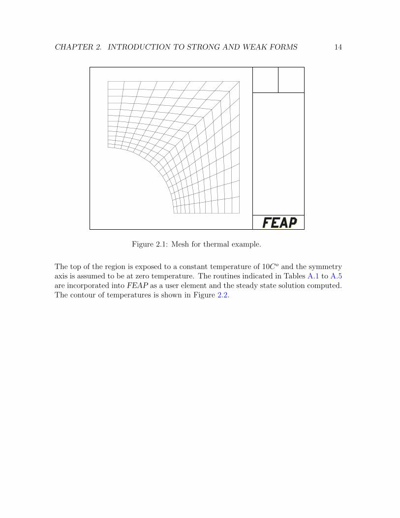
An example of a solution to a problem is the computation of the temperature in arectangular region encasing a circular insulator and subjected to a thermal gradient.The sides of the block are assumed to also be fully insulated. One quadrant of theregion is modeled as shown by the mesh in Figure 2.1.
CHAPTER 2. INTRODUCTION TO STRONG AND WEAK FORMS 14
Figure 2.1: Mesh for thermal example.
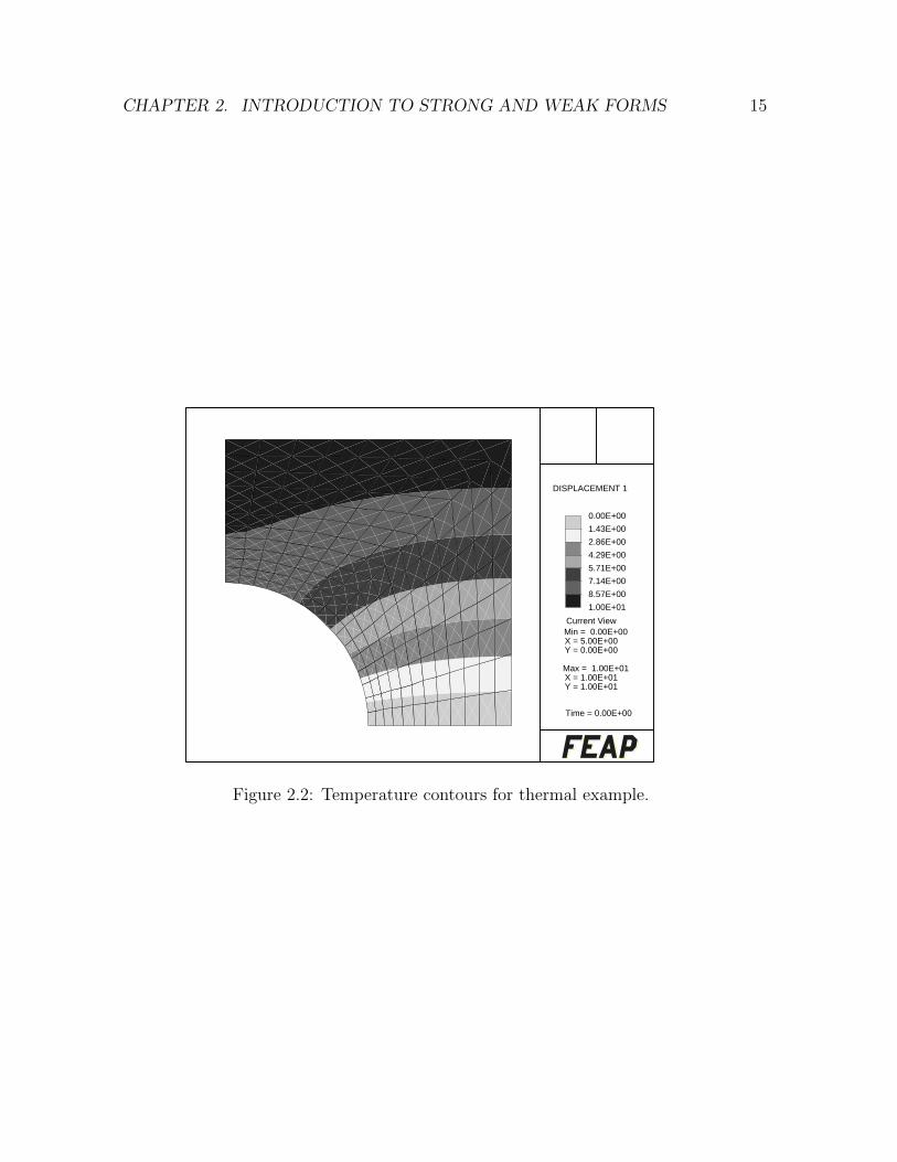
The top of the region is exposed to a constant temperature of 10Co and the symmetryaxis is assumed to be at zero temperature. The routines indicated in Tables A.1 to A.5are incorporated into FEAP as a user element and the steady state solution computed.The contour of temperatures is shown in Figure 2.2.
CHAPTER 2. INTRODUCTION TO STRONG AND WEAK FORMS 15
1.43E+00
2.86E+00
4.29E+00
5.71E+00
7.14E+00
8.57E+00
0.00E+00
1.00E+01
DISPLACEMENT 1
Current ViewMin = 0.00E+00X = 5.00E+00Y = 0.00E+00
Max = 1.00E+01X = 1.00E+01Y = 1.00E+01
Time = 0.00E+00
Figure 2.2: Temperature contours for thermal example.
Chapter 3
Introduction to VariationalTheorems
3.1 Derivatives of functionals: The variation
The weak form of a differential equation is also called a variational equation. Thenotion of a variation is associated with the concept of a derivative of a functional(i.e., a function of functions). In order to construct a derivative of a functional, it isnecessary to introduce a scalar parameter which may be used as the limiting parameterin the derivative[10]. This may be done by introducing a parameter η and defining afamily of functions given by
T η(x) = T (x) + η τ(x) (3.1)
The function τ is an arbitrary function and is related to the arbitrary function Wintroduced in the construction of the weak form. The function ητ is called the variationof the function T and often written as δT (τ(x) alone also may be called the variationof the function)[10].
Introducing the family of functions T η into the functional we obtain, using the steadystate heat equation as an example, the result
Gη = G(W,T η) =
∫Ω
W,i k Tη,i dΩ −
∫Ω
W QdΩ
+
∫Γq
W qn dΓ (3.2)
The derivative of the functional with respect to η now may be constructed using con-ventional methods of calculus. Thus,
dG
dη= lim
η→0
Gη − G0
η(3.3)
16
CHAPTER 3. INTRODUCTION TO VARIATIONAL THEOREMS 17
where G0 is the value of Gη for η equal to 0. The construction of the derivative of thefunctional requires the computation of variations of derivatives of T . Using the abovedefinition we obtain
d(T η),idη
=d
dη(T,i + ητ,i) = τ,i (3.4)
With this result in hand, the derivative of the functional with respect to η is given by
dG
dη=
∫Ω
W,i k τ,i dΩ (3.5)
The limit of the derivative as η goes to zero is called the variation of the functional.For the linear steady state heat equation the derivative with respect to η is constant,hence the derivative is a variation of G. We shall define the derivative of the functionalrepresenting the weak form of a differential equation as
dG
dη= A(W, τ) (3.6)
This is a notation commonly used to define inner products.
3.2 Symmetry of inner products
Symmetry of inner product relations is fundamental to the derivation of variationaltheorems. To investigate symmetry of a functional we consider only terms which includeboth the dependent variable and the arbitrary function. An inner product is symmetricif
A(W, τ) = A(τ,W ) (3.7)
Symmetry of the inner product resulting from the variation of a weak form is a sufficientcondition for the existence of a variational theorem which may also be used to generatea weak form. Symmetry of the functional A also implies that the tangent matrix(computed from the second variation of the theorem or the first variation of the weakform) of a Bubnov-Galerkin finite element method will be symmetric.
A variational theorem, given by a functional Π(T ), has a first variation which is iden-tical to the weak form. Thus, given a functional Π(T ) we can construct G(W,T ) as
limη→0
dΠ(T η)
dη= G(τ, T ) (3.8)
Note that use of Eq. 3.1 leads to a result where τ replaces W in the weak form. Thus,for the variational equation to be equivalent to the weak form τ must be an arbitraryfunction with the same restrictions as we established in defining W . Variational theo-rems are quite common for several problem classes; however, often we may only have a
CHAPTER 3. INTRODUCTION TO VARIATIONAL THEOREMS 18
functional G and desire to know if a variational theorem exists. In practice we seldomneed to have the variational theorem, but knowledge that it exists is helpful since itimplies properties of the discrete problem which are beneficial (e.g., symmetry of thetangent matrices, minimum or stationary value, etc.). Also, existence of a variationaltheorem yields a weak form directly by using Eq. 3.8.
The construction of a variational theorem from a weak form is performed as follows[24]:
1. Check symmetry of the functional A(W, τ). If symmetric then to to 2; otherwise,stop: no varitational theorem exists.
2. Perform the following substitutions in G(W,T )
W (x) → T (x, t) (3.9)
T (x, t) → ηT (x, t) (3.10)
to define G(T, ηT )
3. Integrate the functional result from (b) with respect to η over the interval 0 to 1.
The result of the above process gives
Π(T ) =
∫ 1
0
G(T, ηT )dη (3.11)
Performing the variation of Π and setting to zero gives
limη→0
dΠ(T η)
dη= G(τ, T ) = 0 (3.12)
and a problem commonly referred to as a variational theorem. A variational theoremis a functional whose first variation, when set to zero, yields the governing differentialequations and boundary conditions associated with some problem.
For the steady state heat equation we have
G(T, ηT ) =
∫Ω
T,i k η T,i dΩ −∫
Ω
T QdΩ +
∫Γq
T qn dΓ (3.13)
The integral is trivial and gives
Π(T ) =1
2
∫Ω
T,ikT,idΩ −∫
Ω
TQdΩ +
∫Γq
T qndΓ (3.14)
Reversing the process, the first variation of the variational theorem generates a vari-ational equation which is the weak form of the partial differential equation. The firstvariation is defined by replacing T by
T η = T + ητ (3.15)
CHAPTER 3. INTRODUCTION TO VARIATIONAL THEOREMS 19
and performing the derivative defined by Eq. 3.12. The second variation of the theoremgenerates the inner product
A(τ, τ) (3.16)
If the second variation is strictly positive (i.e., A is positive for all τ), the variationaltheorem is called a minimum principle and the discrete tangent matrix is positive defi-nite. If the second variation can have either positive or negative values the variationaltheorem is a stationary principle and the discrete tangent matrix is indefinite.
The transient heat equation with weak form given by
G =
∫Ω
W(ρ c T − Q
)dΩ +
∫Ω
W,i k T,i dΩ
+
∫Γq
W qn dΓ = 0 (3.17)
does not lead to a variational theorm due to the lack of the symmetry condition forthe transient term
A =(T , ητ
)6= (ητ , T ) (3.18)
If however, we first discretize the transient term using some time integration method,we can often restore symmetry to the functional and then deduce a variational theoremfor the discrete problem. For example if at each time tn we have
T (tn) ≈ Tn (3.19)
then we can approximate the time derivative by the finite difference
T (tn) ≈ Tn+1 − Tntn+1 − tn
(3.20)
Letting tn+1 − tn = ∆t and omitting the subscripts for quantities evaluated at tn+1,the rate term which includes both T and τ becomes
A =
(T
∆t, ητ
)=(ητ
∆t, T)
(3.21)
since scalars can be moved from either term without affecting the value of the term.That is,
A = (T, η τ) = (η T, τ) (3.22)
CHAPTER 3. INTRODUCTION TO VARIATIONAL THEOREMS 20
3.3 Variational notation
A formalism for constructing a variation of a functional may be identified and is similarto constructing the differential of a function. The differential of a function f(xi) maybe written as
df =∂f
∂xidxi (3.23)
where xi are the set of independent variables. Similarly, we may formally write a firstvariation as
δΠ =∂Π
∂uδu +
∂Π
∂u,iδu,i + · · · (3.24)
where u, u,i are the dependent variables of the functional, δu is the variation of thevariable (i.e., it is formally the ητ(x)), and δΠ is called the first variation of the func-tional. This construction is a formal process as the indicated partial derivatives haveno direct definition (indeed the result of the derivative is obtained from Eq. 3.3). How-ever, applying this construction can be formally performed using usual constructionsfor a derivative of a function. For the functional Eq. 3.14, we obtain the result
δΠ =1
2
∫Ω
∂
∂T,i(T,i k T,i) δT,i dΩ −
∫Ω
∂
∂T(T Q) δT dΩ
+
∫Γq
∂
∂T(T qn) δT dΓ (3.25)
Performing the derivatives leads to
δΠ =1
2
∫Ω
(k T,i + T,i k) δT,i dΩ −∫
Ω
QδT dΩ +
∫Γq
qn δT dΓ (3.26)
Collecting terms we have
δΠ =
∫Ω
δT,i k T,i dΩ −∫
Ω
QδT dΩ +
∫Γq
qn δT dΓ (3.27)
which is identical to Eq. 3.2 with δT replacing W , etc.
This formal construction is easy to apply but masks the meaning of a variation. Wemay also use the above process to perform linearizations of variational equations inorder to construct solution processes based on Newton’s method. We shall address thisaspect at a later time.
Chapter 4
Small Deformation: LinearElasticity
A summary of the governing equations for linear elasticity is given below. The equationsare presented using direct notation. For a presentation using indicial notation see [26,Chapter 6]. The presentation below assumes small (infinitesimal) deformations andgeneral three dimensional behavior in a Cartesian coordinate system, x, where thedomain of analysis is Ω with boundary Γ. The dependent variables are given in termsof the displacement vector, u, the stress tensor, σ, and the strain tensor, ε. The basicgoverning equations are:
1. Balance of linear momentum expressed as
∇ · σ + ρbm = ρ u (4.1)
where ρ is the mass density, bm is the body force per unit mass, ∇ is the gradientoperator, and u is the acceleration.
2. Balance of angular momentum, which leads to symmetry of the stress tensor
σ = σT (4.2)
3. Deformation measures based upon the gradient of the displacement vector, ∇u,which may be split as follows
∇u = ∇(s)u + ∇(a)u (4.3)
where the symmetric part is
∇(s)u =1
2
[∇u + (∇u)T
](4.4)
21
CHAPTER 4. SMALL DEFORMATION: LINEAR ELASTICITY 22
and the skew symmetric part is
∇(a)u =1
2
[∇u − (∇u)T
](4.5)
Based upon this split, the symmetric part defines the strain
ε = ∇(s)u (4.6)
and the skew symmetric part defines the spin, or small rotation,
ω = ∇(a)u (4.7)
In a three dimensional setting the above tensors have 9 components. However, ifthe tensor is symmetric only 6 are independent and if the tensor is skew symmetriconly 3 are independent. The component ordering for each of the tensors is givenby
σ →
σ11 σ12 σ13
σ21 σ22 σ23
σ31 σ32 σ33
(4.8)
which from the balance of angular momentum must be symmetric, hence
σij = σji (4.9)
The gradient of the displacement has the components ordered as (with no sym-metries)
∇u →
u1,1 u1,2 u1,3
u2,1 u2,2 u2,3
u3,1 u3,2 u3,3
(4.10)
The strain tensor is the symmetric part with components
ε →
ε11 ε12 ε13
ε21 ε22 ε23
ε31 ε32 ε33
(4.11)
and the symmetry conditionεij = εji (4.12)
The spin tensor is skew symmetric,thus,
ωij = ωji (4.13)
which implies ω11 = ω22 = ω33 = 0. Accordingly,
ω →
ω11 ω12 ω13
ω21 ω22 ω23
ω31 ω32 ω33
=
0 ω12 ω13
−ω12 0 ω23
−ω13 −ω23 0
(4.14)
CHAPTER 4. SMALL DEFORMATION: LINEAR ELASTICITY 23
The basic equations which are independent of material constitution are completed byspecifying the boundary conditions. For this purpose the boundary, Γ, is split into twoparts:
• Specified displacements on the part Γu, given as:
u = u (4.15)
where u is a specified quantity; and
• specified tractions on the part Γt, given as:
t = σn = t (4.16)
where t is a specified quantity.
In the balance of momentum, the body force was specified per unit of mass. This maybe converted to a body force per unit volume (i.e., unit weight/volume) using
ρbm = bv (4.17)
Static or quasi-static problems are considered by omitting the acceleration term fromthe momentum equation (Eq. 4.1). Inclusion of intertial forces requires the specifica-tion of the initial conditions
u(x, 0) = d0(x) (4.18)
u(x, 0) = v0(x) (4.19)
where d0 is the initial displacement field, and v0 is the initial velocity field.
4.1 Constitutive Equations for Linear Elasticity
The linear theory is completed by specifying the constitutive behavior for the material.In small deformation analysis the strain is expressed as an additive sum of parts. Weshall consider several alternatives for splits during the course; however, we begin byconsidering a linear elastic material with an additional known strain. Accordingly,
ε = εm + ε0 (4.20)
where εm is the strain caused by stresses and is called the mechanical part, ε0 is asecond part which we assume is a specified strain. For example, ε0 as a thermal strainis given by
ε0 = εth = α(T − T0) (4.21)
CHAPTER 4. SMALL DEFORMATION: LINEAR ELASTICITY 24
.LP where T is temperature and T0 is a stress free temperature. The constitutiveequations relating stress to mechanical strain may be written (in matrix notation,which is also called Voigt notation) as
σ = Dεm = D(ε − ε0) (4.22)
where the matrix of stresses is ordered as the vector
σ =[σ11 σ22 σ33 σ12 σ23 σ31
]T(4.23)
the matrix of strains is ordered as the vector (note factors of 2 are used to make shearingcomponents the engineering strains, γij)
ε =[ε11 ε22 ε33 2 ε12 2 ε23 2 ε31
]T(4.24)
and D is the matrix of elastic constants given by
D =
D11 D12 D13 D14 D15 D16
D21 D22 D23 D24 D25 D26
D31 D32 D33 D34 D35 D36
D41 D42 D43 D44 D45 D46
D51 D52 D53 D54 D55 D56
D61 D62 D63 D64 D65 D66
(4.25)
Assuming the existence of a strain energy density, W (εm), from which stresses arecomputed as
σab =∂W
∂εmab(4.26)
the elastic modulus matrix is symmetric and satisfies
Dij = Dji (4.27)
Using tensor quantities, the constitutive equation for linear elasticity is written inindicial notation as:
σab = Cabcd(εcd − ε0cd) (4.28)
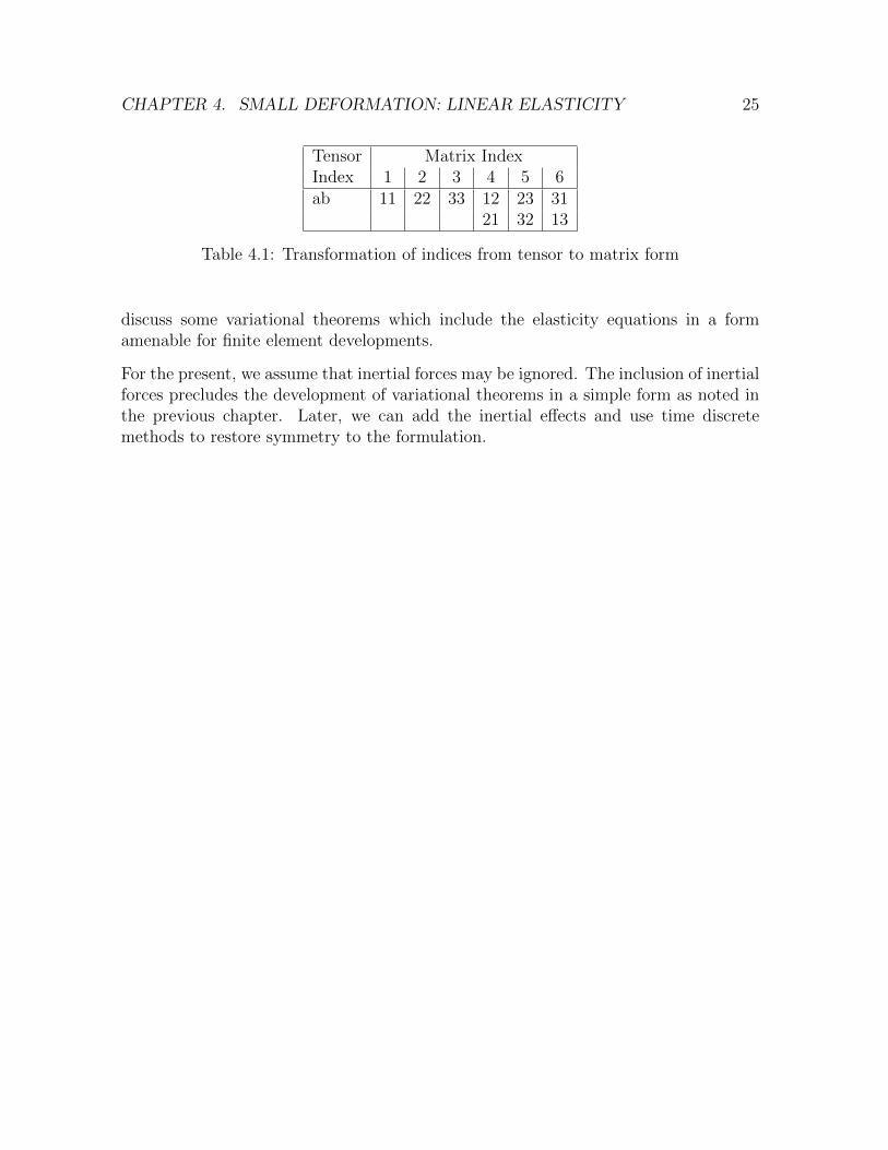
The transformation from the tensor to the matrix (Voigt) form is accomplished by theindex transformations shown in Table 4.1
Thus, using this table, we have
C1111 → D11 ; C1233 → D43 ; etc. (4.29)
The above set of equations defines the governing equations for use in solving linearelastic boundary value problems in which the inertial forces may be ignored. We next
CHAPTER 4. SMALL DEFORMATION: LINEAR ELASTICITY 25
Tensor Matrix IndexIndex 1 2 3 4 5 6ab 11 22 33 12 23 31
21 32 13
Table 4.1: Transformation of indices from tensor to matrix form
discuss some variational theorems which include the elasticity equations in a formamenable for finite element developments.
For the present, we assume that inertial forces may be ignored. The inclusion of inertialforces precludes the development of variational theorems in a simple form as noted inthe previous chapter. Later, we can add the inertial effects and use time discretemethods to restore symmetry to the formulation.
Chapter 5
Variational Theorems: LinearElasticity
5.1 Hu-Washizu Variational Theorem
Instead of constructing the weak form of the equations and then deducing the existenceof a variational theorem, as done for the thermal problem, a variational theorem whichincludes all the equations for the linear theory of elasticity (without inertial forces)will be stated. The variational theorem is a result of the work of the Chinese scholar,Hu, and the Japanese scholar, K. Washizu [25], and, thus, is known as the Hu-Washizuvariational theorem. The theorem may be written as
I(u,σ, ε) =1
2
∫Ω
εT D ε dΩ −∫
Ω
εT D ε0 dΩ
+
∫Ω
σT (∇(s)u − ε) dΩ −∫
Ω
uT bvdΩ
−∫
Γt
uT t dΓ −∫
Γu
tT (u − u)dΓ = Stationary (5.1)
Note that the integral defining the variational theorem is a scalar; hence, a transposemay be introduced into each term without changing the meaning. For example,
I =
∫Ω
aT b dΩ =
∫Ω
(aT b)T dΩ =
∫Ω
bT a dΩ (5.2)
A variational theorem is stationary when the arguments (e.g., u, σ, ε) satisfy the condi-tions where the first variation vanishes. To construct the first variation, we proceed asin the previous chapter. Accordingly, we introduce the variations to the displacement,U, the stress, S, and the strain, E, as
uη = u + ηU (5.3)
26
CHAPTER 5. VARIATIONAL THEOREMS: LINEAR ELASTICITY 27
ση = σ + η S (5.4)
εη = ε + ηE (5.5)
and define the single parameter functional
Iη = I(uη,ση, εη) (5.6)
The first variation is then defined as the derivative of Iη with respect to η and evaluatedat η = 0. For the Hu-Washizu theorem the first variation defining the stationarycondition is given by
dIη
dη
∣∣∣∣η=0
=
∫Ω
ETDεdΩ −∫
Ω
ETDε0dΩ
+
∫Ω
ST (∇(s)u − ε)dΩ +
∫Ω
σT (∇(s)U − E)dΩ
−∫
Ω
UTbvdΩ −∫
Γt
UT tdΓ
−∫
Γu
nTS(u − u)dΓ −∫
Γu
tTUdΓ = 0 (5.7)
The first variation may also be constucted using 3.23 for each of the variables. Theresult is
δI =
∫Ω
δεTDεdΩ −∫
Ω
δεTDε0dΩ
+
∫Ω
δσT (∇(s)u − ε)dΩ +
∫Ω
σT (∇(s)δu − δε)dΩ
−∫
Ω
δuTbvdΩ −∫
Γt
δuT tdΓ
−∫
Γu
nT δσ(u − u)dΓ −∫
Γu
tT δudΓ = 0 (5.8)
and the two forms lead to identical results.
In order to show that the theorem in form 5.7 is equivalent to the equations for linearelasticity, we need to group all the terms together which multiply each variation func-tion (e.g., the U, S, E). To accomplish the grouping it is necessary to integrate byparts the term involving ∇(s)U. Accordingly,∫
Ω
σT∇(s)UdΩ = −∫
Ω
UT∇ · σdΩ +
∫Γt
tTUdΓ +
∫Γu
tTUdΓ (5.9)
CHAPTER 5. VARIATIONAL THEOREMS: LINEAR ELASTICITY 28
Grouping all the terms we obtain
dIη
dη
∣∣∣∣η=0
=
∫Ω
ET [D(ε − ε0) − σ]dΩ
+
∫Ω
ST (∇(s)u − ε)dΩ −∫
Ω
UT (∇ · σ + bv)dΩ
+
∫Γt
UT (t − t)dΓ −∫
Γu
nTS(u − u)dΓ = 0 (5.10)
The fundamental lemma of the calculus of variations states that each expression mul-tiplying an arbitrary function in each integral type must vanish at each point in thedomain of the integral. The lemma is easy to prove. Suppose that an expression doesnot vanish at a point, then, since the variation is arbitrary, we can assume that it isequal to the value of the non-vanishing expression. This results in the integral of thesquare of a function, which must then be positive, and hence the integral will not bezero. This leads to a contradiction, and thus the only possibility is that the assumptionof a non-vanishing expression is false.
The expression which multiplies each variation function is called an Euler equation ofthe variational theorem. For the Hu-Washizu theorem, the variations multiply the con-stitutive equation, the strain-displacement equation, the balance of linear momentum,the traction boundary condition, and the displacement boundary condition. Indeed,the only equation not contained is the balance of angular momentum.
The Hu-Washizu variational principle will serve as the basis for most of what we needin the course. There are other variational principles which can be deduced directlyfrom the principle. Two of these, the Hellinger-Reissner principle and the principleof minimum potential energy are presented below since they are also often used inconstructing finite element formulations in linear elasticity.
5.2 Hellinger-Reissner Variational Theorem
The Hellinger-Reissner principle eliminates the strain as a primary dependent variable;consequently, only the displacement, u, and the stress, σ, remain as arguments inthe functional for which variations are constructed. The strains are eliminated bydeveloping an expression in terms of the stresses. For linear elasticity this leads to
ε = ε0 + D−1σ (5.11)
The need to develop an expression for strains in terms of stresses limits the applicationof the Hellinger-Reissner principle. For example, in finite deformation elasticity thedevelopment of a relation similar to 5.11 is not possible in general. On the other
CHAPTER 5. VARIATIONAL THEOREMS: LINEAR ELASTICITY 29
hand, the Hellinger-Reissner principle is an important limiting case when consideringproblems with constraints (e.g., linear elastic incompressible problems, thin plates asa limit case of the thick Mindlin-Reissner theory). Thus, we shall on occasion use theprinciple in our studies. Introducing 5.11 into the Hu-Washizu principle leads to theresult
I(u,σ) = −1
2
∫Ω
ε0TDε0dΩ − 1
2
∫Ω
σTD−1σdΩ
−∫
Ω
σTε0dΩ +
∫Ω
σT∇(s)udΩ −∫
Ω
uTbvdΩ
−∫
Γt
uT tdΓ −∫
Γu
tT (u − u)dΓ (5.12)
The Euler equations for this principle are
∇(s)u = ε0 + D−1σ (5.13)
together with 4.1, 4.15 and 4.16. The strain-displacement equations are deduced byeither directly stating 4.6 or comparing 5.11 to 5.13. The first term in 5.12 may beomitted since its first variation is zero.
5.3 Minimum Potential Energy Theorem
The principle of minimum potential energy eliminates both the stress, σ, and the strain,ε, as arguments of the functional. In addition, the displacement boundary conditionsare assumed to be imposed as a constraint on the principle. The MPE theorem maybe deduced by assuming
ε = ∇(s)u (5.14)
andu = u (5.15)
are satisfied at each point of Ω and Γ, respectively. Thus, the variational theorem isgiven by the integral functional
I(u) =1
2
∫Ω
(∇(s)u)TD(∇(s)u)dΩ −∫
Ω
(∇(s)u)TDε0dΩ
−∫
Ω
uTbvdΩ −∫
Γt
uT tdΓ (5.16)
Since stress does not appear explicitly in the theorem, the constitutive equation mustbe given. Accordingly, in addition to 5.14 and 5.15 the relation
σ = D(ε − ε0) (5.17)

CHAPTER 5. VARIATIONAL THEOREMS: LINEAR ELASTICITY 30
is given.
The principle of minimum potential energy is often used as the basis for developing adisplacement finite element method.
Chapter 6
Displacement Finite ElementMethods
A variational equation or theorem may be solved using the direct method of the calculusof variations. In the direct method of the calculus of variations the dependent variablesare expressed as a set of trial functions multiplying parameters. This reduces a steadystate problem to an algebraic process and a transient problem to a set of ordinarydifferential equations. In the finite element method we divide the region into elementsand perform the approximations on each element. As indicated in Chapter 2 the regionis divided as
Ω ≈ Ωh =
Mel∑e=1
Ωe (6.1)
and integrals are defined as∫Ω
( · ) dΩ ≈∫
Ωh
( · ) dΩ =
Mel∑e=1
∫Ωe
( · ) dΩ (6.2)
In the above Mel is the total number of elements in the finite element mesh. A similarconstruction is performed for the boundaries. With this construction the parts of thevariational equation or theorem are evaluated element by element.
The finite element approximation for displacements in an element is introduced as
u(ξ, t) =
Nel∑α=1
Nα(ξ) uα(t) = Nα(ξ) uα(t) (6.3)
where Nα is the shape function at node α, ξ are natural coordinates for the element,uα are the values of the displacement vector at node α and repeated indices implysummation over the range of the index. Using the isoparametric concept
31
CHAPTER 6. DISPLACEMENT METHODS 32
x(ξ) = Nα(ξ) xα (6.4)
where xα are the cartesian coordinates of nodes, the displacement at each point in anelement may be computed.
In the next sections we consider the computation of the external force (from appliedloads) and the internal force (from stresses) by the finite element process.
6.1 External Force Computation
In our study we will normally satisfy the displacement boundary conditions u = u bysetting nodal values of the displacement to the values of u evaluated at nodes. Thatis, we express
u = Nα(ξ) uα(t) (6.5)
and set
uα(t) = u(xα, t) (6.6)
We then will assume the integral over Γu is satisfied and may be omitted. This stepis not necessary but is common in most applications. The remaining terms involvingspecified applied loads are due to the body forces, bv, and the applied surface tractions,t. The terms in the variational principal are
Πf =
∫Ωe
uTbv dΩ +
∫Γte
uT t dΓ (6.7)
Using Eq. 6.3 in Eq. 6.7 yields
Πf = (uα)T[∫
Ωe
Nα bv dΩ +
∫Γte
Nα t dΓ
]= (uα)T Fα (6.8)
where Fα denotes the applied nodal force vector at node α and is computed from
Fα =
∫Ωe
Nα bv dΩ +
∫Γte
Nα t dΓ (6.9)
6.2 Internal Force Computation
The stress divergence term in the Hu-Washizu variational principle is generated fromthe variation with respect to the displacements, u, of the term
Πσ =
∫Ωe
(∇(s)u)T σ dΩ =∑e
∫Ωe
(∇(s)u)T σ dΩ (6.10)
CHAPTER 6. DISPLACEMENT METHODS 33
Using the finite element approximation for displacement, the symmetric part of thestrains defined by the symmetric part of the deformation gradient in each element isgiven by
∇(s)u = ε(u) = Bα uα (6.11)
where Bα is the strain displacement matrix for the element. If the components of thestrain for 3-dimensional problems are ordered as
εT =[ε11 ε22 ε33 2 ε12 2 ε23 2 ε31
](6.12)
and related to the displacement derivatives by
εT =[u1,1 u2,2 u3,3 (u1,2 + u2,1) (u2,3 + u3,2) (u3,1 + u1,3)
](6.13)
the strain-displacement matrix is expressed as:
Bα =
Nα,1 0 0
0 Nα,2 00 0 Nα,3
Nα,2 Nα,1 00 Nα,3 Nα,2
Nα,3 0 Nα,1
(6.14)
where
Nα,i =∂Nα
∂xi(6.15)
For a 2-dimensional plane strain problem the non-zero strains reduce to
εT =[ε11 ε22 ε33 2 ε12
](6.16)
and are expressed in terms of the displacement derivatives as
εT =[u1,1 u2,2 0 (u1,2 + u2,1)
](6.17)
thus, Bα becomes:
Bα =
Nα,1 0
0 Nα,2
0 0Nα,2 Nα,1
(6.18)
Finally, for a 2-dimensional axisymmetric problem (with no torsional loading) thestrains are
εT =[ε11 ε22 ε33 2 ε12
](6.19)
and are expressed in terms of the displacements as
εT =[u1,1 u2,2 u1/x1 (u1,2 + u2,1)
](6.20)
CHAPTER 6. DISPLACEMENT METHODS 34
The strain-displacement matrix for axisymmetry, Bα, becomes:
Bα =
Nα,1 0
0 Nα,2
Nα/x1 0Nα,2 Nα,1
(6.21)
where x1, x2 now denote the axisymmetric coordinates r, z, respectively1
The stress divergence term for each element may be written as
Πσe = (uα)T∫
Ωe
(Bα)T σ dΩ (6.22)
In the sequel we define the variation of this term with respect to the nodal displace-ments, uα, the internal stress divergence force. This force is expressed by
Pα(σ) =
∫Ωe
(Bα)T σ dΩ (6.23)
which givesΠσe = (uα)T Pα(σ) (6.24)
The stress divergence term is a basic finite element quantity and must produce aresponse which is free of spurious modes or locking tendencies. Locking is generallyassociated with poor performance at or near the incompressible limit. To study thelocking problem we split the formulation into deviatoric and volumetric terms.
6.3 Split into Deviatoric and Spherical Parts
For problems in mechanics it is common to split the stress and strain tensors into theirdeviatoric and spherical parts. For stress the spherical part is the mean stress definedby
p =1
3tr(σ) =
1
3σkk (6.25)
For infinitesimal strains the spherical part is the volume change defined by
θ = tr(ε) = εkk (6.26)
The deviatoric part of stress , s, is defined so that its trace is zero. The stress may bewritten in terms of the deviatoric and pressure parts (pressure is spherical part) as
σ = s + p1 (6.27)
1For axisymmetry it is also necessary to replace the volume element by dΩ → x1 dx1 dx2 and thesurface element by dΓ → x1 dS where dS is an boundary differential in the x1 - x2 plane.
CHAPTER 6. DISPLACEMENT METHODS 35
where, 1 is the rank two identity tensor, which in matrix notation is given by the vector
mT =[1 1 1 0 0 0
](6.28)
In matrix form the pressure is given by
p =1
3mT σ (6.29)
thus, the deviatoric part of stresses now may be computed as
s = σ − 1
3m mT σ =
(I − 1
3m mT
)σ (6.30)
where, in three dimensions, I is a 6× 6 identity matrix. We note that the trace of thestress gives
mT σ = 3 p = mT s + pmT m = mT s + 3 p (6.31)
and hencemT s = 0 (6.32)
as required.
For subsequent developments, we define
Idev = I − 1
3m mT (6.33)
as the deviatoric projector. Similarly, the volumetric projector is defined by
Ivol =1
3m mT (6.34)
These operators have the following properties
I = Idev + Ivol (6.35)
Idev = Idev Idev = (Idev)m (6.36)
Ivol = Ivol Ivol = (Ivol)m (6.37)
andIvol Idev = Idev Ivol = 0 (6.38)
In the above m is any positive integer power. We note, however, that inverses to theprojectors do not exist.
Utilizing the above properties, we can operate on the strain to define its deviatoric andvolumetric parts. Accordingly, the deviatoric and volumetric parts are given by
ε = e +1
3θ 1 (6.39)
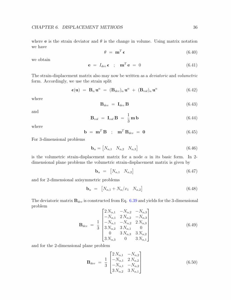
CHAPTER 6. DISPLACEMENT METHODS 36
where e is the strain deviator and θ is the change in volume. Using matrix notationwe have
θ = mT ε (6.40)
we obtaine = Idev ε ; mT e = 0 (6.41)
The strain-displacement matrix also may now be written as a deviatoric and volumetricform. Accordingly, we use the strain split
ε(u) = Bα uα = (Bdev)α uα + (Bvol)α uα (6.42)
whereBdev = Idev B (6.43)
and
Bvol = Ivol B =1
3m b (6.44)
whereb = mT B ; mT Bdev = 0 (6.45)
For 3-dimensional problems
bα =[Nα,1 Nα,2 Nα,3
](6.46)
is the volumetric strain-displacement matrix for a node α in its basic form. In 2-dimensional plane problems the volumetric strain-displacement matrix is given by
bα =[Nα,1 Nα,2
](6.47)
and for 2-dimensional axisymmetric problems
bα =[Nα,1 +Nα/x1 Nα,2
](6.48)
The deviatoric matrix Bdev is constructed from Eq. 6.39 and yields for the 3-dimensionalproblem
Bdev =1
3
2Nα,1 −Nα,2 −Nα,3
−Nα,1 2Nα,2 −Nα,3
−Nα,1 −Nα,2 2Nα,3
3Nα,2 3Nα,1 00 3Nα,3 3Nα,2
3Nα,3 0 3Nα,1
(6.49)
and for the 2-dimensional plane problem
Bdev =1
3
2Nα,1 −Nα,2
−Nα,1 2Nα,2
−Nα,1 −Nα,2
3Nα,2 3Nα,1
(6.50)
CHAPTER 6. DISPLACEMENT METHODS 37
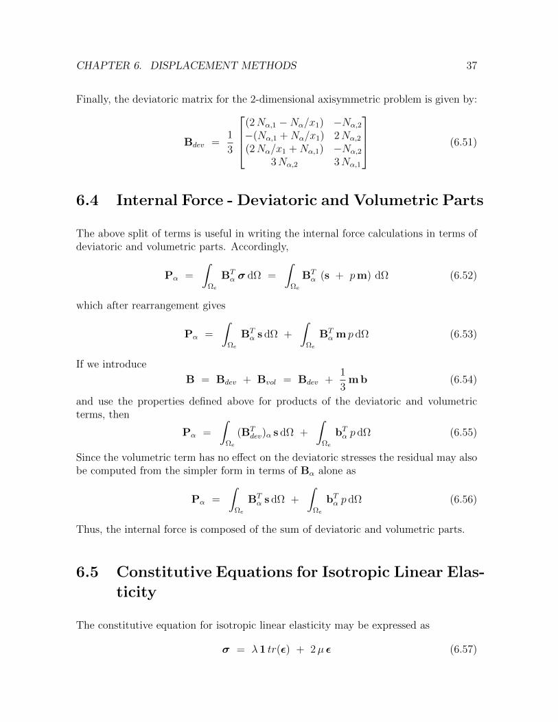
Finally, the deviatoric matrix for the 2-dimensional axisymmetric problem is given by:
Bdev =1
3
(2Nα,1 −Nα/x1) −Nα,2
−(Nα,1 +Nα/x1) 2Nα,2
(2Nα/x1 +Nα,1) −Nα,2
3Nα,2 3Nα,1
(6.51)
6.4 Internal Force - Deviatoric and Volumetric Parts
The above split of terms is useful in writing the internal force calculations in terms ofdeviatoric and volumetric parts. Accordingly,
Pα =
∫Ωe
BTα σ dΩ =
∫Ωe
BTα (s + pm) dΩ (6.52)
which after rearrangement gives
Pα =
∫Ωe
BTα s dΩ +
∫Ωe
BTα m p dΩ (6.53)
If we introduce
B = Bdev + Bvol = Bdev +1
3m b (6.54)
and use the properties defined above for products of the deviatoric and volumetricterms, then
Pα =
∫Ωe
(BTdev)α s dΩ +
∫Ωe
bTα p dΩ (6.55)
Since the volumetric term has no effect on the deviatoric stresses the residual may alsobe computed from the simpler form in terms of Bα alone as
Pα =
∫Ωe
BTα s dΩ +
∫Ωe
bTα p dΩ (6.56)
Thus, the internal force is composed of the sum of deviatoric and volumetric parts.
6.5 Constitutive Equations for Isotropic Linear Elas-
ticity
The constitutive equation for isotropic linear elasticity may be expressed as
σ = λ1 tr(ε) + 2µ ε (6.57)
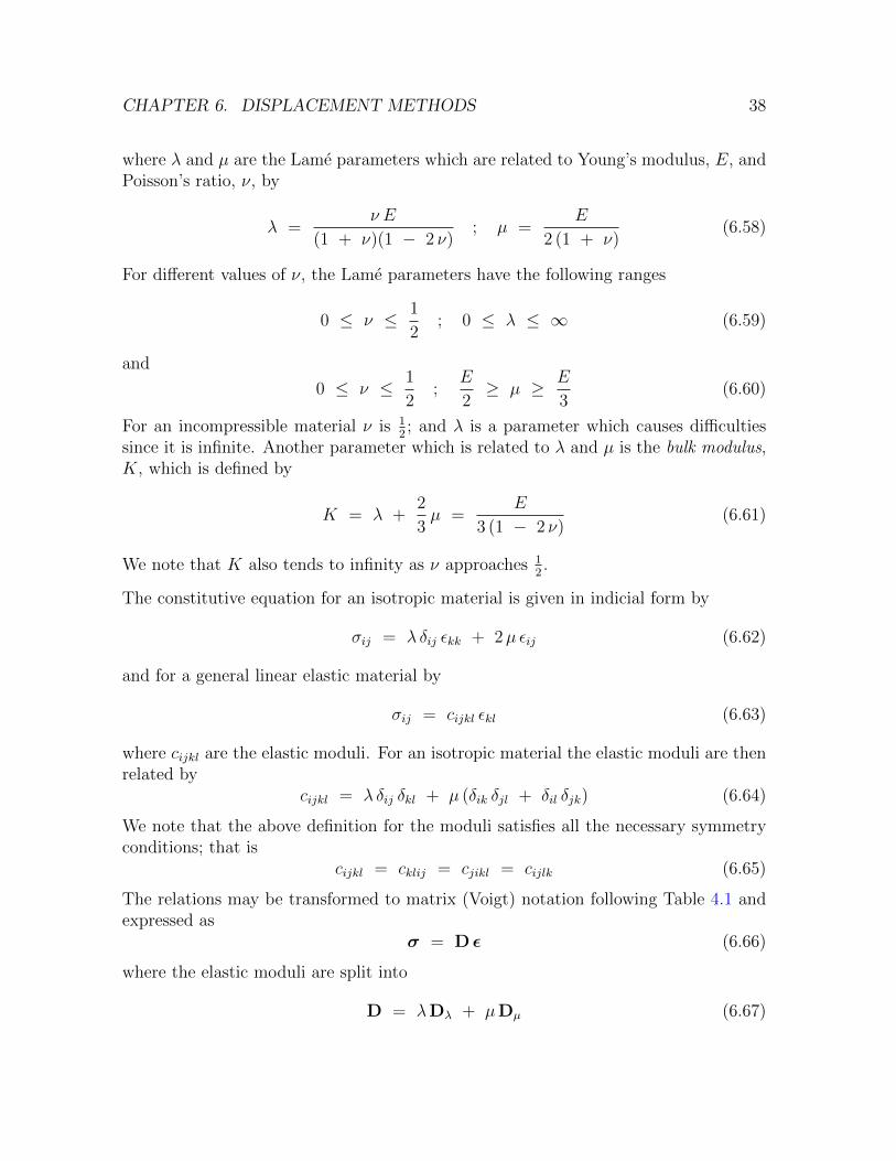
CHAPTER 6. DISPLACEMENT METHODS 38
where λ and µ are the Lame parameters which are related to Young’s modulus, E, andPoisson’s ratio, ν, by
λ =ν E
(1 + ν)(1 − 2 ν); µ =
E
2 (1 + ν)(6.58)
For different values of ν, the Lame parameters have the following ranges
0 ≤ ν ≤ 1
2; 0 ≤ λ ≤ ∞ (6.59)
and
0 ≤ ν ≤ 1
2;
E
2≥ µ ≥ E
3(6.60)
For an incompressible material ν is 12; and λ is a parameter which causes difficulties
since it is infinite. Another parameter which is related to λ and µ is the bulk modulus,K, which is defined by
K = λ +2
3µ =
E
3 (1 − 2 ν)(6.61)
We note that K also tends to infinity as ν approaches 12.
The constitutive equation for an isotropic material is given in indicial form by
σij = λ δij εkk + 2µ εij (6.62)
and for a general linear elastic material by
σij = cijkl εkl (6.63)
where cijkl are the elastic moduli. For an isotropic material the elastic moduli are thenrelated by
cijkl = λ δij δkl + µ (δik δjl + δil δjk) (6.64)
We note that the above definition for the moduli satisfies all the necessary symmetryconditions; that is
cijkl = cklij = cjikl = cijlk (6.65)
The relations may be transformed to matrix (Voigt) notation following Table 4.1 andexpressed as
σ = D ε (6.66)
where the elastic moduli are split into
D = λDλ + µDµ (6.67)
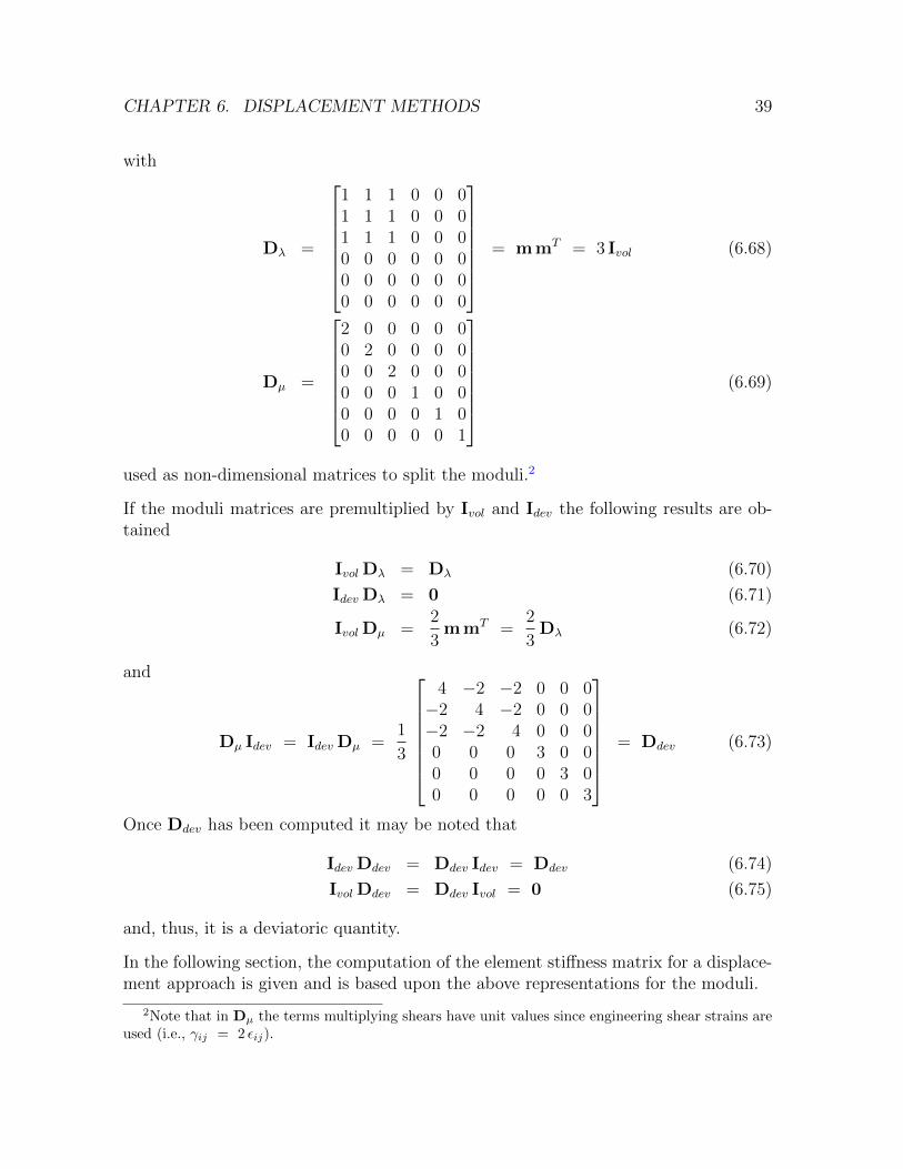
CHAPTER 6. DISPLACEMENT METHODS 39
with
Dλ =
1 1 1 0 0 01 1 1 0 0 01 1 1 0 0 00 0 0 0 0 00 0 0 0 0 00 0 0 0 0 0
= m mT = 3 Ivol (6.68)
Dµ =
2 0 0 0 0 00 2 0 0 0 00 0 2 0 0 00 0 0 1 0 00 0 0 0 1 00 0 0 0 0 1
(6.69)
used as non-dimensional matrices to split the moduli.2
If the moduli matrices are premultiplied by Ivol and Idev the following results are ob-tained
Ivol Dλ = Dλ (6.70)
Idev Dλ = 0 (6.71)
Ivol Dµ =2
3m mT =
2
3Dλ (6.72)
and
Dµ Idev = Idev Dµ =1
3
4 −2 −2 0 0 0−2 4 −2 0 0 0−2 −2 4 0 0 00 0 0 3 0 00 0 0 0 3 00 0 0 0 0 3
= Ddev (6.73)
Once Ddev has been computed it may be noted that
Idev Ddev = Ddev Idev = Ddev (6.74)
Ivol Ddev = Ddev Ivol = 0 (6.75)
and, thus, it is a deviatoric quantity.
In the following section, the computation of the element stiffness matrix for a displace-ment approach is given and is based upon the above representations for the moduli.
2Note that in Dµ the terms multiplying shears have unit values since engineering shear strains areused (i.e., γij = 2 εij).
CHAPTER 6. DISPLACEMENT METHODS 40
6.6 Stiffness for Displacement Formulation
The displacement formulation is accomplished for a linear elastic material by notingthat the constitutive equation is given by (for simplicity ε0 is assumed to be zero)
σ = D ε (6.76)
The strains for a displacement approach are given by
ε = Bβ uβ (6.77)
where uβ are the displacements at node β.
Constructing the deviatoric and volumetric parts may be accomplished by writing
s = Idev σ = Idev D ε = Idev(λDλ + µDµ)ε (6.78)
andpm = Ivol D ε = Ivol(λDλ + µDµ)ε (6.79)
If we use the properties of the moduli multiplied by the projectors, the above equationsreduce to
s = µDdev ε = µDµ e = µDµ(Bdev)β uβ (6.80)
and
pm = (λ +2
3µ) Dλ ε = K Dλ ε = K m(mT ε) = K m θ (6.81)
Thus, the pressure constitutive equation is
p = K θ (6.82)
Noting that the volumetric strain may be computed from
θ = bβ uβ (6.83)
the pressure for the displacement model may be computed from
p = K bβ uβ (6.84)
We recall from Section 6.2 that
Pα =
∫Ωe
(BTdev)α s dΩ +
∫Ωe
bTα p dΩ (6.85)
Using the above definitions and identities the internal force vector may be written as
Pα =
∫Ωe
µ (BTdev)α Dµ (Bdev)β dΩ uβ +
∫Ωe
K bα bTβ dΩ uβ (6.86)
CHAPTER 6. DISPLACEMENT METHODS 41
and, thus, for isotropic linear elasticity, the stiffness matrix may be deduced as thesum of the deviatoric and volumetric parts
Kαβ = (Kdev)αβ + (Kvol)αβ (6.87)
where
(Kdev)αβ =
∫Ωe
µ (BTdev)α Dµ (Bdev)β dΩ =
∫Ωe
µBTα Ddev Bβ dΩ (6.88)
and
(Kvol)αβ =
∫Ωe
K bα bTβ dΩ =
∫Ωe
K BTα Dλ Bβ dΩ (6.89)
6.7 Numerical Integration
Generally the computation of integrals for the finite element arrays is performed us-ing numerical integration (i.e., quadrature). The use of the same quadrature for eachpart of the stress divergence terms given above (in P and K) leads to a conventionaldisplacement approach for numerically integrated finite element developments. Theminimum order quadrature which produces a stiffness with the correct rank (i.e., num-ber of element degree-of-freedoms less the number of rigid body modes) will be calleda standard or full quadrature (or integration). The next lowest order of quadrature iscalled a reduced quadrature. Alternatively, use of standard quadrature on one term andreduced quadrature on another leads to a method called selective reduced quadrature.
A typical integral is evaluated by first transforming the integral onto a natural coordi-nate space ∫
Ωe
f(x) dΩ =
∫2
f(x(ξ)) j(ξ) dξ (6.90)
where∫2
denotes integration over the natural coordinates ξ, dξ denotes dξ1dξ2 in2-dimensions, and j(ξ) is the determinant of the jacobian transformation
J(ξ) =∂x
∂ξ(6.91)
Thusj(ξ) = detJ(ξ) (6.92)
The integrals over 2 are approximated using a quadrature formula, thus∫2
f(x(ξ)) j(ξ) dξ ≈L∑l=1
f(x(ξl)) j(ξl)wl (6.93)
CHAPTER 6. DISPLACEMENT METHODS 42
where ξl and wl are quadrature points and quadrature weights, respectively. For brickelements in three dimensions and quadrilateral elements in two dimensions, the inte-gration is generally carried out as a product of one-dimensional Gaussian quadrature.Thus, for 2-dimensions, ∫
2
g(ξ) dξ =
∫ 1
−1
∫ 1
−1
g(ξ) dξ1 dξ2 (6.94)
and for 3-dimensions ∫2
g(ξ) dξ =
∫ 1
−1
∫ 1
−1
∫ 1
−1
g(ξ) dξ1 dξ2 dξ3 (6.95)
Using quadrature, the stress divergence is given by
Pα =L∑l=1
Bα(ξl)T σ(ξl) j(ξl)wl (6.96)
and the stiffness matrix is computed by quadrature as
Kαβ =L∑l=1
Bα(ξl)T D (ξl)Bβ(ξl) j(ξl)wl (6.97)
Similar expressions may be deduced for each of the terms defined by the deviatoric/volu-metric splits. The use of quadrature reduces the development of finite element arraysto an algebraic process involving matrix operations. For example, the basic algorithmto compute the stress divergence term is given by:
1. Initialize the array Pα
2. Loop over the quadrature points, l
• Compute j(ξl)wl = c
• Compute the matrix in the integrand, (e.g., Bα(ξl)T σl = Aα).
• Accumulate the array, e.g.,
Pα ← Pα + Aα c (6.98)
3. Repeat step 2 until all quadrature points in element are considered.
Additional steps are involved in computing the entries in each array. For example, thedetermination of Bα requires computation of the derivatives of the shape functions,Nα,i, and computation of σl requires an evaluation of the constitutive equation at thequadrature point. The evaluation of the shape functions is performed using a shapefunction subprogram. In FEAP, a shape function routine for 2 dimensions is calledshp2d and is accessed by the call
CHAPTER 6. DISPLACEMENT METHODS 43
call shp2d( xi, xl, shp, xsj, ndm, nel, ix, flag)
where
xi natural coordinate values (ξ1, ξ2) at quadraturepoint (input)
xl array of nodal coordinates for element(xl(ndm,nen)) (input)
shp array of shape functions and derivatives(shp(3,nen)) (output)
xsj jacobian determinant at quadrature point(output)
ndm spatial dimension of problems (input)nel number of nodes on element (between 3 and
9) (input)ix array of global node numbers on element
(ix(nen)) (input)flag flag, if false derivatives returned with
respect to x (input); if truederivatives returned with respect to ξ.
The array of shape functions has the following meanings:
shp(1,A) is NA,1
shp(2,A) is NA,2
shp(3,A) is NA,3
The quadrature points may be obtained by a call to int2d:
call int2d( l, lint, swg )
where
l -number of quadrature points in each direction(input).
lint -total number of quadrature points (output).swg -array of natural coordinates and weights (output).
The array of points and weights has the following meanings:
CHAPTER 6. DISPLACEMENT METHODS 44
swg(1,L) is ξ1,L
swg(2,L) is ξ2,L
swg(3,L) is wL
Using the above two utility subprograms a 2-dimensional formulation for displacement(or mixed) finite element method can be easily developed for FEAP. An example, iselement elmt01 which is given in Appendix B.
Chapter 7
Mixed Finite Element Methods
7.1 Solutions using the Hu-Washizu Variational The-
orem
A finite element formulation which is free from locking at the incompressible or nearlyincompressible limit may be developed from a mixed variational approach. In the workconsidered here we use the Hu-Washizu variational principle, which we recall may bewritten as
Π(u,σ, ε) =1
2
∫Ω
εT D ε dΩ −∫
Ω
εT D ε0 dΩ
+
∫Ω
σT (∇(s)u − ε) dΩ −∫
Ω
uTbv dΩ
−∫
Γt
uT t dΓ −∫
Γu
tT (u − u) dΓ = Stationary (7.1)
In the principle, displacements appear up to first derivatives, while the stresses andstrains appear without any derivatives. Accordingly, the continuity conditions we mayuse in finite element approximations are C0 for the displacements and C−1 for thestresses and strains (a C−1 function is one whose first integral will be continuous).Appropriate interpolations for each element are thus
u(ξ) = NI(ξ) uI(t) (7.2)
σ(ξ) = φα(ξ)σα(t) (7.3)
andε(ξ) = ψα(ξ) εα(t) (7.4)
45
CHAPTER 7. MIXED FINITE ELEMENT METHODS 46
where φα(ξ) and ψα(ξ) are interpolations which are continuous in each element butmay be discontinuous across element boundaries.1 The parameters σα and εα are notnecessarily nodal values and, thus, may have no direct physical meaning.
If, for the present, we ignore the integral for the body force, and the traction anddisplacement boundary integrals and consider an isotropic linear elastic material, theremaining terms may be split into deviatoric and volumetric parts as
Π(u,σ, ε) =1
2
∫Ω
µ εT Ddev ε dΩ −∫
Ω
µ εT Ddev ε0 dΩ
+
∫Ω
sT [e(u) − e] dΩ (7.5)
+1
2
∫Ω
K θ2 dΩ −∫
Ω
K θ θ0 dΩ +
∫Ω
p[θ(u) − θ] dΩ
wheree(u) = Idev∇(s)u (7.6)
andθ(u) = tr(∇(s)u) = ∇ · u (7.7)
are the strain-displacement relations for the deviatoric and volumetric parts, respec-tively.
Constructing the variation for the above split leads to the following Euler equationswhich hold in the domain Ω:
1. Balance of Momentum
∇ · (s + 1 p) + bv = 0 (7.8)
which is also written as
div(s + 1 p) + bv = 0 (7.9)
2. Strain-Displacement equations
e(u) − e = 0 (7.10)
θ(u) − θ = 0 (7.11)
3. Constitutive equationsµDdev ε − s = 0 (7.12)
K θ − p = 0 (7.13)
1Strictly, φα and ψα need only be piecewise continuous in each element; however, this makes theevaluation of integrals over each element more difficult and to date is rarely used.
CHAPTER 7. MIXED FINITE ELEMENT METHODS 47
In addition the boundary conditions for Γu and Γt are obtained.
Using the interpolations described above, the Hu-Washizu variational theorem may beapproximated by summing the integrals over each element. Accordingly,
Π(u,σ, ε) ≈ Πh(u,σ, ε) =∑e
Πe(u,σ, ε) (7.14)
If the deviatoric part is approximated by taking
e = e(u) (7.15)
for each point of Ω, this part of the problem is given as a displacement model. Thevariational expression Eq. 7.5 becomes
Π(u, p, θ) =1
2
∫Ω
µ εT (u) Ddev ε(u) dΩ −∫
Ω
µ εT (u) Ddev ε0 dΩ
+1
2
∫Ω
K θ2 dΩ −∫
Ω
K θ θ0 dΩ
+
∫Ω
p [θ(u) − θ] dΩ (7.16)
which may be split into integrals over the elements as
Π(u, p, θ) ≈ Πh(u, p, θ) =∑e
Πe(u, p, θ) (7.17)
A mixed approximation may now be used to describe the pressure and the volumechange in each element. Accordingly, we assume
p(ξ) = φα(ξ) pα(t) = φ(ξ) p (7.18)
θ(ξ) = φα(ξ) θα(t) = φ(ξ)θ (7.19)
where it is noted that the same approximating functions are used for both p and theta.If the material is isotropic linear elastic, the use of the same functions will permit anexact satisfaction of the constitutive equation, Eq. 7.13 at each point of the domain ofan element. For other situations, the constitutive equation may be approximately sat-isfied. Recall that the strain-displacement equations for a finite element approximationare given by
ε(u) = BI uI (7.20)
Thus, the finite element approximation for the mixed formulation may be written as
Πe(u,p,θ) = (uI)T[
1
2
∫Ωe
µBTI Ddev BJ dΩ uJ −
∫Ωe
µBTI Ddev ε
0 dΩ
]+ θT
[1
2
∫Ωe
K φT φ dΩθ −∫
Ωe
K φT θ0 dΩ
]+ pT
[ ∫Ωe
φT bJ dΩ uJ −∫
Ωe
φT φ dΩθ
](7.21)
CHAPTER 7. MIXED FINITE ELEMENT METHODS 48
If we define the following matrices:
k =
∫Ωe
K φT φ dΩ (7.22)
π0 =
∫Ωe
K φT θ0 dΩ (7.23)
h =
∫Ωe
φT φ dΩ (7.24)
gI =
∫Ωe
φT bI dΩ (7.25)
and recall that the deviatoric stiffness is defined as
(Kdev)IJ =
∫Ωe
BTI Ddev BJ dΩ (7.26)
and denote the effects of initial deviatoric strains as
(P0dev)I =
∫Ωe
µBTI Ddev ε
0 dΩ =
∫Ωe
µBTI Dµ e0 dΩ (7.27)
where e0 are the deviatoric initial strains. The mixed variational terms become
Πe(u,p,θ) = (uI)T[
1
2(Kdev)IJ uJ − (P0
dev)I
]+ θT
[1
2kθ − π0
]+ pT
[gJ uJ − hθ
](7.28)
If we denote the variations of pressure and volume change as
pη = p + ηΠ (7.29)
θη = θ + ηΘ (7.30)
the first variation of Eq. 7.28 may be written in the matrix form
dΠe
dη=
[(UI)T ,ΠT ,ΘT
] (Kdev)IJ gJ 0gTI 0 −h0 −h k
uJ
pθ
−
(P0dev)I0π0
(7.31)
CHAPTER 7. MIXED FINITE ELEMENT METHODS 49
or in variational notation as
δΠe =[(δuI)T , δpT , δθT
] (Kdev)IJ gJ 0gTI 0 −h0 −h k
uJ
pθ
−
(P0dev)I0π0
(7.32)
We note that the parameters p and θ (and their variations Π and Θ) are associatedwith a single element, consequently, from the stationarity condition, the last two rowsof the above matrix expression must vanish and may be solved at the element level.The requirement for a solution to exist is that2
nθ ≥ np (7.33)
where nθ and np are the number of parameters associated with the volume change andpressure approximations, respectively. We have satisfied this requirement by takingan equal number for the two approximations. Also, since we used the same functionsfor the two approximations, the matrix h is square and positive definite (provided ourapproximating functions are linearly independent), consequently, we may perform theelement solutions by inverting only h. The solution to Eq. 7.32 is
θ = h−1 gJ uJ (7.34)
and the solution to the third row is
p = h−1(kθ − π0) (7.35)
Substitution of the above results into the first equation gives
dΠe
dη= (UI)T
([(Kdev)IJ + gTI h−1 k h−1 gJ
]uJ
− (P0dev)I − gTI h−1 π0
)(7.36)
Finally, by defining a modified volumetric strain-displacement matrix as
bI = h−1 gJ (7.37)
the above simplifies to
dΠe
dη= (UI)T
[((Kdev)IJ + bTI k bJ
)uJ − (P0
dev)I − bTI π0]
(7.38)
2This is a mixed patch test requirement. See [26, Chapter 12].
CHAPTER 7. MIXED FINITE ELEMENT METHODS 50
The volumetric stiffness for the mixed formulation is given as
(Kvol)IJ = bTI k bJ (7.39)
and the volumetric initial force by
(P0vol)I = bTI π
0 (7.40)
The stress divergence term for the mixed model formulation is computed from
PI =
∫Ωe
BTI (s + pm) dΩ (7.41)
where the deviatoric stress is expressed by the displacement approximation as
s = µDdev(BJ uJ − ε0) (7.42)
and the pressure is expressed by the mixed approximation as
p = φ(ξ) h−1 (kθ − π0) (7.43)
7.2 Finite Element Solution for Mixed Formulation
The mixed finite element solution for the linear elastic problem requires selecting a setof approximating functions for φ. The number of φ functions will affect the rank ofthe volumetric terms. The modified volumetric stiffness has a rank which is given by
rank(Kvol) = min ( rank(b), rank(k) ) (7.44)
Provided the approximations for φ are linearly independent, and the number is smallcompared to the number of degrees-of-freedom on the element, the rank will normallybe that of k. For example, 4-node quadrilateral or 8-node brick elements can use asingle function
φ1 = 1 (7.45)
for the approximating space. This gives a rank of 1 for the volumetric stiffness. Therequirement for the approximation is guided by the principle that: (1) we use theminimum number of functions which make K have correct rank for a single element,and (2) the functions produce an element which is invariant with respect to the inputdata. For example, if we show that two functions are sufficient for a 2-dimensionalelement, use of
φ1 = 1 ; φ2 = ξ1 (7.46)
CHAPTER 7. MIXED FINITE ELEMENT METHODS 51
would not be good since the element is not invariant with respect to a permutation inthe definition of ξ1 and ξ2. Several alternatives are possible, one being
φ1 = 1 ; φ2 = ξ1 + ξ2 (7.47)
another is to use 3 functions with
φ1 = 1 ; φ2 = ξ1 ; φ3 = ξ2 (7.48)
The actual functions selected must be subjected to further evaluations to decide whichbest meets the objectives of the problem solution.
An algorithm to implement the above mixed model for linear elasticity where D isconstant in each element may be summarized as:
1. Initialize arrays: gI , h, k, π0. FEAP will initialize K and the element residual.
2. Loop over quadrature points, l
(a) Compute shape functions: In 2-d problems FEAP uses,
NI(ξl) = shp(3, I, l) (7.49)
NI , i(ξl) = shp(i, I, l) (7.50)
(b) Compute the volume element times the quadrature weight
jl wl = dv(l) (7.51)
3. Loop over quadrature points, l
(a) Compute the volumetric strain matrices, gI and h.
4. Invert h and compute bIbI = h−1gI (7.52)
5. Loop over quadrature points, l
(a) Compute strain-displacement matrix, B, and strains, ε
εl = [Idev BI(ξl) +1
3mφ(ξl) bI ] u
I (7.53)
(b) Compute quadrature stresses and π0
σl = D (εl − ε0) (7.54)
CHAPTER 7. MIXED FINITE ELEMENT METHODS 52
(c) Compute the residual
RI = FI −lint∑l=1
BTI (ξl)σl j(ξl)Wl (7.55)
(d) Compute the deviatoric tangent, Kdev
(e) Compute the volumetric local tangent, k
6. Compute the tangent, K
K = Kdev + bT k b (7.56)
7.3 Mixed Solutions for Anisotropic Linear Elastic
Materials
A more general form of the Hu-Washizu principle is needed to consider either anisotropiclinear elastic materials or inelastic materials in which there is coupling between volu-metric and deviatoric effects. In this section we construct the form of the functionalfor an anisotropic linear elastic material. Accordingly, we have
σ = D [ε − ε0] (7.57)
where D is a symmetric matrix in which there may be coupling between the deviatoricand volumetric strain effects. It is now assumed that a finite element solution will beconstructed in which deviatoric strains, e, are computed directly from the displace-ments but the volumetric strain, θ, is computed from a mixed form. Accordingly,
ε = Idev ε(u) +1
3m θ (7.58)
A stress may be computed from ε as
σ = D [Idev (ε(u) − ε0) +1
3m (θ − θ0)] (7.59)
where θ0 = mTε0. The stress may be split into deviatoric and pressure parts as
σ = s + m p (7.60)
where
s = Idev D [Idev (ε(u) − ε0) +1
3m (θ − θ0)] (7.61)
and
p =1
3mT D [Idev (ε(u) − ε0) +
1
3m (θ − θ0)] (7.62)
CHAPTER 7. MIXED FINITE ELEMENT METHODS 53
If we defineDdev = Idev D Idev (7.63)
d =1
3Idev D m (7.64)
dvol =1
9mT D m (7.65)
s0 = − Ddev ε0 − d θ0 (7.66)
andp0 = − dT ε0 − dvol θ
0 (7.67)
then the stress may be written as
σ = Ddev ε(u) + d θ +1
3m (dTε(u) + dvol θ) + s0 + m p0 (7.68)
This form of the stress may be multiplied by the virtual ε and integrated over thedomain to obtain part of the variational equation associated with the strain energy.Subsequently, adding the terms associated with the mixed volumetric pressure andvolume change Vainberg’s theorem may be used to obtain a variational theorem. Al-ternatively, the stress and strain splits may be substituted into 7.1. The result is
Π(u, p, θ) =1
2
∫Ω
[ε(u) θ
] [Ddev ddT dvol
] [ε(u)θ
]dΩ
+
∫Ω
(ε(u) s0 + θ p0) dΩ
+
∫Ω
p [θ(u) − θ] dΩ + Πext (7.69)
This form of the variational principle is equivalent to 7.16 which was deduced forisotropic materials. The added terms in 7.69 are all associated with d which defines acoupling between deviatoric and volumetric strains. For isotropy d is zero.
If we introduce finite element interpolations using standard displacement interpolationtogether with the pressure and volume interpolations given by 7.18 and 7.19, the firstvariation of 7.69 for a single element is
δΠe =[δuTI δθ
T] ∫
Ωe
[BTI DdevBJ BT
I dφφTdTBJ φTdvolφ
] [uJθ
]+
[BTI s0
φTp0
]dΩ + δpT
∫Ωe
φT[bJ −φ
]dΩ
[uJθ
]+
[δuTI δθ
T] ∫
Ωe
[bTI φ−φTφ
]dΩ p + δIext (7.70)
CHAPTER 7. MIXED FINITE ELEMENT METHODS 54
The variational equation 7.70 may be expressed in terms of stresses by substituting theinterpolations into 7.61 and 7.62 resulting in
δΠe =[δuTI δθ
T] ∫
Ωe
[BTI s
φT p
]dΩ
+ δpT∫
Ωe
φT[bJ −φ
]dΩ
[uJθ
]+
[δuTI δθ
T] ∫
Ωe
[bTI φ−φTφ
]dΩ p + δIext (7.71)
Since the interpolations for the pressure and volume change are associated with a singleelement it is possible to solve for their parameters at the element level. Accordingly,the multiple of δp yields∫
Ωe
φT bJ dΩ uJ =
∫Ωe
φT φ dΩ θ = h θ (7.72)
which yieldsθ = bI uI = h−1gI uI (7.73)
where h and gI are as defined in 7.24 and 7.25, respectively. similarly, the equationmultiplying δθ yields the equation∫
Ωe
φT p dΩ =
∫Ωe
φT φ dΩ p = h p (7.74)
Using these results, the first integral in the variational equation defines the stressdivergence terms
δΠσ = δuTI
[∫Ω
BTI s dΩ + bTI
∫Ω
φT p dΩ
](7.75)
which upon use of the definitions for the mixed pressure, p, and the mixed volumetricstrain displacement equation, bI , yields
δΠσ = δuTI
∫Ω
BTI [s + m p] dΩ (7.76)
The stress of the mixed method is defined as
σ = s + m p (7.77)
and, in general, is not equal to σ. The stress σ, however, is the stress which is computedfrom the constitutive equation for each material. Thus, when we later consider othermaterial models (e.g., viscoelasticity, plasticity, etc.) the effective material moduli arethe ones computed by linearizing the constitutive equation expressed in terms of the
CHAPTER 7. MIXED FINITE ELEMENT METHODS 55
σ stresses. The residual for a finite element formulation is most efficiently computedfrom the mixed stress and we note the result is identical to the form of the standarddisplacement model except for the stress expression used.
The tangent matrix may be expressed in terms of the displacements alone by writingthe variational equation 7.70 as
δΠe =[δuTI δθ
TδpT
] (Kdev)IJ kI gJkTJ kvol −hgTI −h 0
uIθp
+ δΠ0 + δΠext (7.78)
Using the solutions to 7.72 and 7.74 the dependence of 7.78 on θ and p may beeliminated to give
δΠe = δuTI KIJ uJ + δΠ0 + δΠext (7.79)
whereKIJ = (Kdev)IJ + kIbJ + bTI kTJ + bTI kvolbJ (7.80)
The algorithm for the development of a mixed element based upon the above may besummarized as:
1. Numerical integration of strain matrices
(a) Compute φ = [1, ξ1, ξ2, · · · ] (for the 4-node element φ = 1
(b) Compute arrays
h =
∫Ωe
φTφ dΩ (7.81)
gI =
∫Ωe
φTbJ dΩ (7.82)
2. Mixed volumetric strain displacement matrix
(a) Compute bI = h−1gI
3. Constitution computation for each quadrature point
(a) Computeε = BI uI (7.83)
θ = φ(ξ) bI uI (7.84)
ε = Idev ε +1
3m θ (7.85)
σ = D[ε − ε0] (7.86)
CHAPTER 7. MIXED FINITE ELEMENT METHODS 56
p =1
3mT σ (7.87)
π =
∫Ωe
φT p dΩ (7.88)
4. Mixed Pressure
(a) Compute p = φ(ξ) h−1 π
5. Residual and Stiffness Integrals
(a) Compute mixed stress σ = Idev σ + m p
(b) Compute
RσI = −
∫Ωe
BTI σ dΩ (7.89)
(Kdev)IJ =
∫Ωe
BTI Ddev Bd
JΩ (7.90)
kI =
∫Ωe
BTI dφ dΩ (7.91)
kvol =
∫Ωe
φT dvol φ dΩ (7.92)
6. Stiffness assembly
(a) Compute
KIJ = (Kdev)IJ + kIbJ + bTI kTJ + bTI kvol bJ (7.93)
7.4 Hu-Washizu Variational Theorem: General Prob-
lems
The finite element approximation for the mixed formulation of a general linear elasticmaterial (i.e., anistotropic behavior) may be written for a typical element as
Πe(u,p,θ) =1
2
∫Ωe
εT D ε dΩ −∫
Ωe
εT D ε0 dΩ
+ p (∇ · u − θ) dΩ (7.94)
Using the approximations introduced for the isotropic model for the displacement andmixed volume change gives
ε = Idev BI uI +1
3mφ(ξ)θ (7.95)
CHAPTER 7. MIXED FINITE ELEMENT METHODS 57
which when introduced into the variational theorem gives
Πe(u,p,θ) =1
2
∫Ωe
[Idev BI uI +
1
3mφ(ξ)θ
]TD[Idev BI uI
+1
3mφ(ξ)θ
]dΩ −
∫Ωe
[Idev BI uI +
1
3mφ(ξ)θ
]TD ε0 dΩ
+ pT[ ∫
Ωe
φT bJ dΩ uJ −∫
Ωe
φT φ dΩθ
](7.96)
For symmetric D, we can define the following matrices:
(Kdev)IJ =
∫Ωe
BTI Idev D Idev BJ dΩ (7.97)
(Kco)J =1
3
∫Ωe
φT mT D Idev BJ dΩ (7.98)
k =1
9
∫Ωe
φT mT D mφ dΩ (7.99)
π0 =1
3
∫Ωe
φT m D ε0 dΩ (7.100)
h =
∫Ωe
φT φ dΩ (7.101)
gI =
∫Ωe
φT bI dΩ (7.102)
and denote the effects of initial deviatoric strains as
(P0dev)I =
∫Ωe
BTI Idev D ε0 dΩ (7.103)
The mixed variational terms become
Πe(u,p,θ) =1
2[(uI)T (Kdev)IJ uJ + 2θT (Kco)J uJ + θT kθ]
− (uI)T (P0dev)I − θT π0 + pT gI uI − pT hθ (7.104)
The first variation of Eq. 7.104 may be written in the matrix form
dΠe
dη=
[(UI)T ,ΠT ,ΘT
] (Kdev)IJ gI (Kco)IgTJ 0 −h
(KTco)J −h k
uJ
pθ
−
(P0dev)I0π0
(7.105)
CHAPTER 7. MIXED FINITE ELEMENT METHODS 58
Recall that the terms which multiply the variations in pressure, Π, and the variation inthe volume change, Θ, are associated with individual elements, and, thus, the secondrow of Eq. 7.105 may be solved at the element level to give the parameters for thevolume change, θ, as
θ = h−1 gJ uJ (7.106)
and the solution to the third row is
p = h−1[(Kco)J uJ + kθ − π0] (7.107)
Defining a modified volumetric strain-displacement matrix as
bI = h−1 gJ (7.108)
Substitution of the above results into the first equation gives
dΠe
dη= (UI)T
([(Kdev)IJ + bTI (Kco)J + (KT
co)IbJ + bTI k bJ]
uJ
− (P0dev)I − bTI π
0)
(7.109)
Thus, the stiffness matrix for the general anisotropic linear elastic formulation is givenby
KIJ = (Kdev)IJ + bTI (Kco)J + (KTco)IbJ + bTI k bJ (7.110)
This operation may be performed after all the integrals over the element are evaluated.
The matrices which involve the elastic moduli may be simplified by defining somereduced terms. Accordingly, we let3
d =1
3D m (7.112)
Also, define
dvol =1
9mTD m =
1
3mT d (7.113)
ThenD Idev = D − d mT (7.114)
orIdev D = D − m dT (7.115)
3If D is not symmetric, equations Eq.7.112 through Eq.7.117 must be modified. Essentially, thisrequires a computation of two d terms as
dR = Dm ; dL = DT m (7.111)
and using these in the remaining equations instead of d (note, when D is symmetric the dR and dLterms are equal).
CHAPTER 7. MIXED FINITE ELEMENT METHODS 59
which gives
1
3Idev D m =
1
3(D − m dT ) m = d − dvol m = ddev (7.116)
Finally, the deviatoric part of the modulus is now defined in terms of the above as
Ddev = Idev D Idev = D − d mT − m dT + dvol m mT (7.117)
For isotropy, the above expressions reduce to:
dvol = K (7.118)
d =[K K K 0 0 0
]T(7.119)
ddev = 0 (7.120)
and
Ddev =1
3µ
4 −2 −2 0 0 0−2 4 −2 0 0 0−2 −2 4 0 0 00 0 0 3 0 00 0 0 0 3 00 0 0 0 0 3
(7.121)
The matrices for the mixed treatment of the symmetric D anisotropic case are com-puted as:
(Kdev)IJ =
∫Ωe
BTI Ddev BJ dΩ (7.122)
(Kco)J =
∫Ωe
φT dTdev BJ dΩ (7.123)
and
k =
∫Ωe
dvol φT φ dΩ (7.124)
The matrix for the initial strains is computed as
π0 =
∫Ωe
φT dT ε0 dΩ (7.125)
which is a 1× 6 vector.
CHAPTER 7. MIXED FINITE ELEMENT METHODS 60
7.4.1 Example: Interpolations linear for u and constant φ
As an example, we consider the case where the set of shape functions for the displace-ments is the tri-linear interpolation
NI(ξ) =1
8(1 + ξI1 ξ1) (1 + ξI2 ξ2) (1 + ξI3 ξ3) (7.126)
where ξIi are the values of the natural coordinates at the I-node. The interpolation forthe pressure (and volume change) is constant
φ1 = 1 (7.127)
This element is often called B1-P0 (order 1 interpolations for the brick element, order 0for the pressure/volume change). In 2-dimensions the element is Q1-P0, for the order 1quadrilateral. Higher order elements are also defined, for example, the Q2-P1 elementuses quadratic interpolation for displacements (Lagrange interpolations) and linear forthe pressure with
φ(ξ) =[1 ξ1 ξ2
](7.128)
Alternatively, it is possible to use the interpolations
φ(ξ) =[1 x1(ξ) x2(ξ)
](7.129)
The matrices for the B1-P0 (or Q1-P0) element reduce to
(Kco)J =
∫Ωe
dTdev BJ dΩ (7.130)
which is a column vector (of size 1× 24). For isotropy, this matrix is zero. The volumestiffness becomes:
k =
∫Ωe
dvol dΩ (7.131)
which is a 1× 1 matrix and for constant dvol becomes
k = kvol = dvol Ωe (7.132)
where Ωe is the volume of the element. For isotropy kvol is the bulk modulus times theelement volume. The other matrices in the stiffness are
h = h =
∫Ωe
dΩ = Ωe (7.133)
and
gI =
∫Ωe
bI dΩ (7.134)
CHAPTER 7. MIXED FINITE ELEMENT METHODS 61
which gives the modified volumetric strain-displacement equation
bI =1
Ωe
gI =1
Ωe
∫Ωe
bI dΩ (7.135)
The initial strain term is computed as
π0 =
∫Ωe
dT ε0 dΩ (7.136)
For the mixed element the internal force is computed using
PI =
∫Ωe
BTI (s(u) + pm) dΩ (7.137)
where the deviatoric part of the stress is computed from the displacement form, andthe pressure is computed from the mixed form
p =1
Ωe
([(Kco)J + kvol bJ ] uJ − π0
)(7.138)
Chapter 8
Enhanced Strain Mixed Method
8.1 Hu-Washizu Variational Theorem for Linear Elas-
ticity
An alternative to the mixed finite element method discussed previously is given bythe enhanced strain method [16]. The enhanced strain method is related to earlierworks which utilized incompatible displacement modes; however, the method does nothave the deficiencies which are present in the earlier works. Enhanced strains providegreat flexibility in designing accurate finite element models for problems which haveconstraints or other similar types of difficulties. In the enhanced strain method weagain use the Hu-Washizu variational principle, which we recall may be written forlinear elasticity as
Π(u,σ, ε =1
2
∫Ω
εT D ε dΩ −∫
Ω
εT D ε0 dΩ
+
∫Ω
σT (∇(s)u − ε) dΩ −∫
Ω
uTbv dΩ
−∫
Γt
uT t dΓ −∫
Γu
tT (u − u) dΓ = Stationary (8.1)
The strain tensor is expressed as an additive sum of the symmetric gradient of thedisplacement vector, ∇(s)u, and the enhanced strains, ε, and written as
ε(u, ε) = ∇(s)u + ε(ξ) (8.2)
62
CHAPTER 8. ENHANCED STRAIN MIXED METHOD 63
If we again ignore the integral for the body force and the traction and displacementboundary integrals, upon use of Eq. 8.2 the remaining terms become
Π(u,σ, ε) =1
2
∫Ω
(∇(s)u + ε)T D (∇(s)u + ε) dΩ
−∫
Ω
(∇(s)u + ε)T D ε0 dΩ −∫
Ω
σT ε dΩ (8.3)
Introducing the variations for each function as
uη = u + ηU (8.4)
ση = σ + η S (8.5)
andεη = ε + η E (8.6)
the variation for the above enhanced principle is given by
dΠ
dη=
∫Ω
(∇(s)U)T D (∇(s)u + ε − ε0) dΩ
+
∫Ω
ET [D (∇(s)u + ε − ε0) − σ] dΩ −∫
Ω
ST ε dΩ (8.7)
After integration by parts of the variation of the displacement gradient term (and alsoconsidering the body force term), the following Euler equations are obtained for thedomain Ω:
1. Balance of momentum
div [D (∇(s)u + ε − ε0)] + bv = 0 (8.8)
2. Strain-displacement equations on the enhanced modes
ε = 0 (8.9)
3. Constitutive equations
D (∇(s)u + ε − ε0) − σ = 0 (8.10)
In addition the boundary conditions for Γu and Γt are obtained. We note Eq. 8.9implies that, at the solution, the enhanced strains must vanish. Substitution of thisresult into the remaining equations yields the appropriate displacement equations ofequilibrium and constitutive equation for linear elasticity, from 8.8 and 8.10, respec-tively. While the enhanced strains vanish pointwise at a solution, in an approximate
CHAPTER 8. ENHANCED STRAIN MIXED METHOD 64
scheme based upon the enhanced strain method this is not the case. The enhancedstrains will only vanish in some integral sense over each element, just as the balance ofmomentum and constitutive equations are approximated by finite element solutions.
In the enhanced strain principle, displacements appear up to first derivatives, whilethe stresses and enhanced strains appear without any derivatives. Accordingly, thecontinuity conditions we may use in finite element approximations again are C0 for thedisplacements and C−1 for the stresses and enhanced strains. Appropriate interpola-tions for displacements and stresses are the same as given previously for each element,and are thus
u(ξ) = NI(ξ) uI(t) (8.11)
andσ(ξ) = φα(ξ)σα(t) (8.12)
respectively. The choice of appropriate approximating functions φα will be affected bythe strain approximation, as will be shown below. From Eq. 8.2, the strain approxi-mations are now given by
ε(u, ε) = ∇(s)u + ε(ξ) (8.13)
where the approximations for the enhanced strains are assumed as
ε(ξ) = ψα(ξ) εα(t) (8.14)
It should be noted that different interpolations are introduced for the stress and theenhanced strain terms.
Using the interpolations described above, the Hu-Washizu variational theorem may beapproximated by summing the integrals over each element. Accordingly,
Π(u,σ, ε) = Πh(u,σ, ε) ≈∑e
Πe(u,σ, ε) (8.15)
The variational expression in each element becomes
Πe(u,σ, ε) =1
2
∫Ωe
(∇(s)u + ε)T D (∇(s)u + ε) dΩ
−∫
Ωe
(∇(s)u + ε)T D ε0 dΩ −∫
Ωe
σT ε dΩ (8.16)
Substituting the approximations for displacements, stresses, and enhanced strains andreplacing with
uIη = uI + ηUI (8.17)
σαη = σα + η Sα (8.18)
andεαη = εα + η Eα (8.19)
CHAPTER 8. ENHANCED STRAIN MIXED METHOD 65
gives the first variation in each element as
dΠe
dη=[
(UI)T , (Eα)T , (Sα)T]KIJ ΓβI 0
ΓT
αJ Hαβ Qαβ
0 QTβα 0
uJ
εβ
σβ
−P0
I
π0α
0
(8.20)
where
KIJ =
∫Ωe
BTI D BJ dΩ (8.21)
ΓαJ =
∫Ωe
ψTα D BJ dΩ (8.22)
Hαβ =
∫Ωe
ψTα Dψβ dΩ (8.23)
Qαβ =
∫Ωe
φTα ψβ dΩ (8.24)
P0I =
∫Ωe
BTI D ε0 dΩ (8.25)
π0α =
∫Ωe
ψTα D ε0 dΩ (8.26)
The discrete Euler equation generated by the third equation of Eq. 8.20 is given ineach element by
Qαβ εβ = 0 (8.27)
There are at least three possible ways this may be used:
1. The εβ are zero, which is not a useful result.
2. The interpolations for φα are orthogonal to the interpolations ψβ, which meansthat
Qαβ = 0 (8.28)
which is the solution to be followed here. This is not perfect since we will notobtain a method to compute the σβ directly from the variational formulation.
3. A combination of options (a) and (b).
For a formulation which satisfies Eq. 8.28, the variational equations in each elementreduce to
dΠe
dη=[
(UI)T , (Eα)T]([KIJ ΓβI
ΓT
αJ Hαβ
] [uJ
εβ
]−[P0I
π0α
])(8.29)
CHAPTER 8. ENHANCED STRAIN MIXED METHOD 66
Since the interpolations for the enhanced strains are assumed for each element inde-pendently, the second of Eq. 8.29 may be solved at the element level giving
εβ = (Hαβ)−1[π0α − ΓαJ uJ
](8.30)
which may be substituted into the first equation to give
dΠe
dη= (UI)T KIJ uJ − P0
I (8.31)
whereKIJ = KIJ − Γ
T
βI (Hαβ)−1 ΓαJ (8.32)
andP0I = P0
I − ΓT
βI (Hαβ)−1 π0α (8.33)
8.2 Stresses in the Enhanced Method
Since the stresses based upon the mixed approximation are no longer available analternative is needed for computations. Simo and Rifai suggest using a least squareprojection technique to obtain the stresses; however, the stresses which are directlyutilized in the variational equation Eq. 8.7 may be deduced as
σ = D (∇(s)u + ε − ε0) (8.34)
In subsequent development we shall use these stresses for all calculations of arrays, aswell as, for outputs and stress projections to nodes. Thus, the variation in each elementmay be written
dΠe
dη
∣∣∣∣η=0
=
∫Ωe
(∇(s)U)T σ dΩ +
∫Ωe
ET σ dΩ (8.35)
It is noted that the orthogonality condition∫Ωe
ST ε dΩ = 0 (8.36)
has been incorporated in the above variation.
With the above description, the residual in each element becomes:
RI = FI −∫
Ωe
BTI σ dΩ (8.37)
CHAPTER 8. ENHANCED STRAIN MIXED METHOD 67
for the contribution in the element to the global residual. Similarly, the residual forthe enhanced modes is computed from
Rα = −∫
Ωe
ψTα σ dΩ (8.38)
Note that the residual for the enhanced modes will vanish at a solution since it belongsto a single element.
8.3 Construction of Enhanced Modes
The construction of the enhanced modes depends crucially on the orthogonality require-ment being satisfied for each element. Based upon the study of the shape functionsusing the alternative representation we recall that the gradient of the displacementinvolves a constant part and a part which depends only on the determinant of the jaco-bian matrix, j(ξ), the constant part of the jacobian matrix, J0, and gradients of localcoordinates, ξ. Accordingly, it is useful to express the enhanced strains in a similarform. Using tensor notation we introduce the representations
ε =j0
j(ξ)J−T0 E(ξ) J−1
0 (8.39)
which represents a transformation of the local enhanced strains, E, expressed on thebi-unit square to the global strains, ε, using the transformation defined at the elementcenter. The weighting by the jacobian determinant terms is motivated by the gradientof the shape functions. Similarly, a transformation of the local stresses, Σ, on thebi-unit square element to the global stresses, σ, is given by
σ = J0 Σ(ξ) JT0 (8.40)
These transformations have the property that
tr(σ ε) =j0
j(ξ)tr(Σ E) (8.41)
The transformations may also be written in matrix form as
ε =j0j(ξ)
F−10 E(ξ) (8.42)
σ =j0
j(ξ)FT
0 Σ(ξ) (8.43)
where for 2-dimensional problems
ET =[E11 E22 E33 2 E12
](8.44)
CHAPTER 8. ENHANCED STRAIN MIXED METHOD 68
ΣT =[Σ11 Σ22 Σ33 Σ12
](8.45)
and ε and σ have similar ordering. The matrix F0 is given by
F0 =
(J11
0 )2 J210 J
120 0 2 J11
0 J120
J120 J
210 (J22
0 )2 0 2 J210 J
220
0 0 1 0J11
0 J210 J12
0 J220 0 J11
0 J220 + J12
0 J210
(8.46)
In matrix form Eq. 8.41 may be written as
σT ε =j0
j(ξ)ΣT E (8.47)
The integral over the element becomes∫Ωe
σT ε dΩ = j0
∫2
ΣT E d2 = 0 (8.48)
Thus, the satisfaction of the orthogonality condition may be accomplished by con-structing the interpolations in the natural coordinate system and transforming to theglobal frame using Eq. 8.42 and Eq. 8.43. A number of alternatives are discussed inthe paper by Simo and Rifai [16]. Here we consider the simplest form, which indeed isidentical to the modified incompatible mode formulation [22]. It should be noted how-ever, that no ad-hoc assumptions are required in the enhanced formulation, contraryto what is necessary when using incompatible modes.
For the simplest form, the interpolations
Σ =
1 0 0 00 1 0 00 0 1 00 0 0 1
Σ1
Σ2
Σ3
Σ4
(8.49)
for the stress and
E =
ξ1 0 0 00 ξ2 0 00 0 0 00 0 ξ1 ξ2
E1
E2
E3
E4
(8.50)
for the enhanced strains are used. The integrals of natural coordinates over the bi-linear(2-dimensional) element obey the following properties∫
2
ξpi d2 =
0 if p odd
4p+1
if p even(8.51)
Thus, the interpolations given by Eqs. 8.49 and Eqs. 8.50 contain only linear polyno-mials in ξ and, thus, satisfy the orthogonality condition Eq. 8.48. These interpolationshave been incorporated into the element routine elmt04 which has been developed fora linear elastic-viscoelastic material, as well as, for non-linear materials.
CHAPTER 8. ENHANCED STRAIN MIXED METHOD 69
8.4 Non-Linear Elasticity
For a non-linear, hyperelastic material the stresses are computed from a strain energydensity function, W (ε), through
σ =∂W
∂ε(8.52)
The partial derivative is understood in terms of components, where
σij =∂W
∂εij(8.53)
We note that for the linear material model discussed previously that
W (ε) =1
2εT D ε − εT D ε0 (8.54)
For the enhanced formulation the computation of stresses is given by
σ =∂W
∂ε
∣∣∣∣ε = ∇(s)u + ε
(8.55)
In subsequent development we shall use these stresses for all calculations of arrays, aswell as, for outputs and stress projections to nodes. Thus, for the enhanced formulationthe variation in each element may be written as (see Eqs. 8.35 to 8.38)
dΠe
dη=
∫Ωe
(∇(s)U)T σ dΩ +
∫Ωe
ET σ dΩ (8.56)
In a manner identical to the linear elastic material, the residual in each element be-comes:
RI = FI −∫
Ωe
BTI σ dΩ (8.57)
Similarly, the residual for the enhanced modes is computed from
Rα = −∫
Ωe
ψTα σ dΩ = 0 (8.58)
We note above that at a solution the residual, Rα, should vanish independently in eachelement.
8.5 Solution Strategy: Newton’s Method
The solution to a non-linear problem is commonly computed using a sequence of linearapproximations. A popular scheme is Newton’s method, which may be summarized as:
CHAPTER 8. ENHANCED STRAIN MIXED METHOD 70
1. Given the set of equationsf(x) = 0 (8.59)
where x are the dependent variables.
2. Construct the linear part of f about a current point x(i) as
f (i+1) ≈ f (i) +∂f
∂x
∣∣∣∣x=x(i)
dx(i+1) = 0 (8.60)
where dx(i+1) is an increment of x.
3. Solve the linear problem
dx(i+1) = − (F(i))−1 f (i) ; F(i) =∂f
∂x
∣∣∣∣x=x(i)
(8.61)
and update the solution as
x(i+1) = x(i) + dx(i+1) (8.62)
In the above, F(i), is the Jacobian or tangent matrix for the equations.
4. Repeat steps b.) and c.) until the solution converges to within a tolerance, tol.Convergence may be assessed from
| dx(i+1) | < tol | x(i+1) | (8.63)
where | x | is the length of the vector, x.
Using Newton’s method on the set of equations defined by Eq. 8.57 and Eq. 8.58 abovegives the problem[
R(i+1)I
R(i+1)α
]≈
[R
(i)I
R(i)α
]−
[K
(i)IJ Γ
(i)
βI
Γ(i)
αJT H(i)αβ
] [duJ(i+1)
dεβ(i+1)
]=
[R
(i+1)I
0
](8.64)
In the above, the terms in the Jacobian are defined as
K(i)IJ = − ∂RI
∂uJ
∣∣∣∣(i) (8.65)
which expands to
K(i)IJ =
∫Ωe
BI∂σ
∂ε
∣∣∣∣(i) ∂ε
∂uJdΩ =
∫Ωe
BI D(i)t BJ dΩ (8.66)
CHAPTER 8. ENHANCED STRAIN MIXED METHOD 71
where
D(i)t =
∂σ
∂ε
∣∣∣∣(i) (8.67)
define the tangent moduli for the material. For the non-linear elastic material
D(i)t =
∂2W
∂ε ∂ε
∣∣∣∣(i) (8.68)
Similarly,
Γ(i)
αJ =
∫Ωe
ψTα D
(i)t BJ dΩ (8.69)
and
H(i)αβ =
∫Ωe
ψTα D
(i)t ψβ dΩ (8.70)
Since the second equation in Eq. 8.64 is complete at the element level, we may performa partial solution by static condensation. Accordingly,
dεβ(i+1) = (H(i)αβ)−1 [R(i)
α − Γ(i)
αJ duJ(i+1)] (8.71)
which may be substituted into the first equation to give
R(i+1)I = R
(i)I − K
(i)IJ du
J(i+1) (8.72)
whereR
(i)I = R
(i)I − Γ
(i)
βIT (H(i)αβ)−1 R(i)
α (8.73)
andK
(i)IJ = K
(i)IJ − Γ
(i)T
βI (H(i)αβ)−1 Γ
(i)
αJ (8.74)
The reduced first equations may be assembled into the global equations. Thus afteradding any nodal forces, FI , the assembled equations become∑
e
K(i)IJ du
J(i+1) =∑e
R(i)I + FI (8.75)
which may be solved for the incremental nodal displacements, duJ(i+1). After the solve,the new nodal displacements are updated
uJ(i+1) = uJ(i) + duJ(i+1) (8.76)
The incremental displacements also may be substituted back into Eq. 8.71 to computethe increments to the enhanced modes; these may then be used for the update
εβ(i+1) = εβ(i) + dεβ(i+1) (8.77)
CHAPTER 8. ENHANCED STRAIN MIXED METHOD 72
It should be noted that these last steps may not be performed until after the elementarrays are assembled and the resulting global problem is solved for the incrementalnodal displacements. Consequently, for this algorithm, it is necessary to save thearrays used in Eq. 8.71 for the later update of the enhanced modes. In the enhancedelement for 2-dimensional plane strain applications in FEAP, the arrays are moved intohistory arrays using a pmove routine. This requires additional storage for the enhancedformulation with respect to that needed for a displacement or a mixed B-bar type offormulation. It is possible to modify the above algorithm such that the additionalstorage is reduced to saving only the current values of the enhanced mode parameters,εβ(i).
The alternate algorithm is given by linearizing the residual, Rα, with respect to εβ only.Accordingly, with uJ(i) known we enter each element calculation with the enhancedstrain parameters at the values εβ(i−1) and perform the following steps.
1. For k = 0 setεβ(i,k) = εβ(i−1) (8.78)
where a single superscript i denotes the value of εβ computed in the last globaliteration.
2. Compute the linear part of Rα as
Rα(uJ(i), εβ(i,k)) − H(i,k)αβ dεβ(i,k+1) = 0 (8.79)
where now
H(i,k)αβ =
∫Ωe
ψTα D
(i,k)t ψβ dΩ (8.80)
with
D(i,k)t =
∂σ
∂ε
∣∣∣∣∇(s)u(i) + ε(i,k)
(8.81)
3. Solve for the increment
dεβ(i,k+1) = (H(i,k)αβ )−1 R(i,k)
α (8.82)
4. Update the solutionεβ(i,k+1) = εβ(i,k) + dεβ(i,k+1) (8.83)
5. Set k ← k + 1 and repeat Steps 2. to 4. until convergence achieved (or a setnumber of k-steps is completed).
6. Setεβ(i) = εβ(i,k+1) (8.84)
and save for the next global iteration, as well as use for subsequent steps for theglobal i-iterations or to compute stresses.
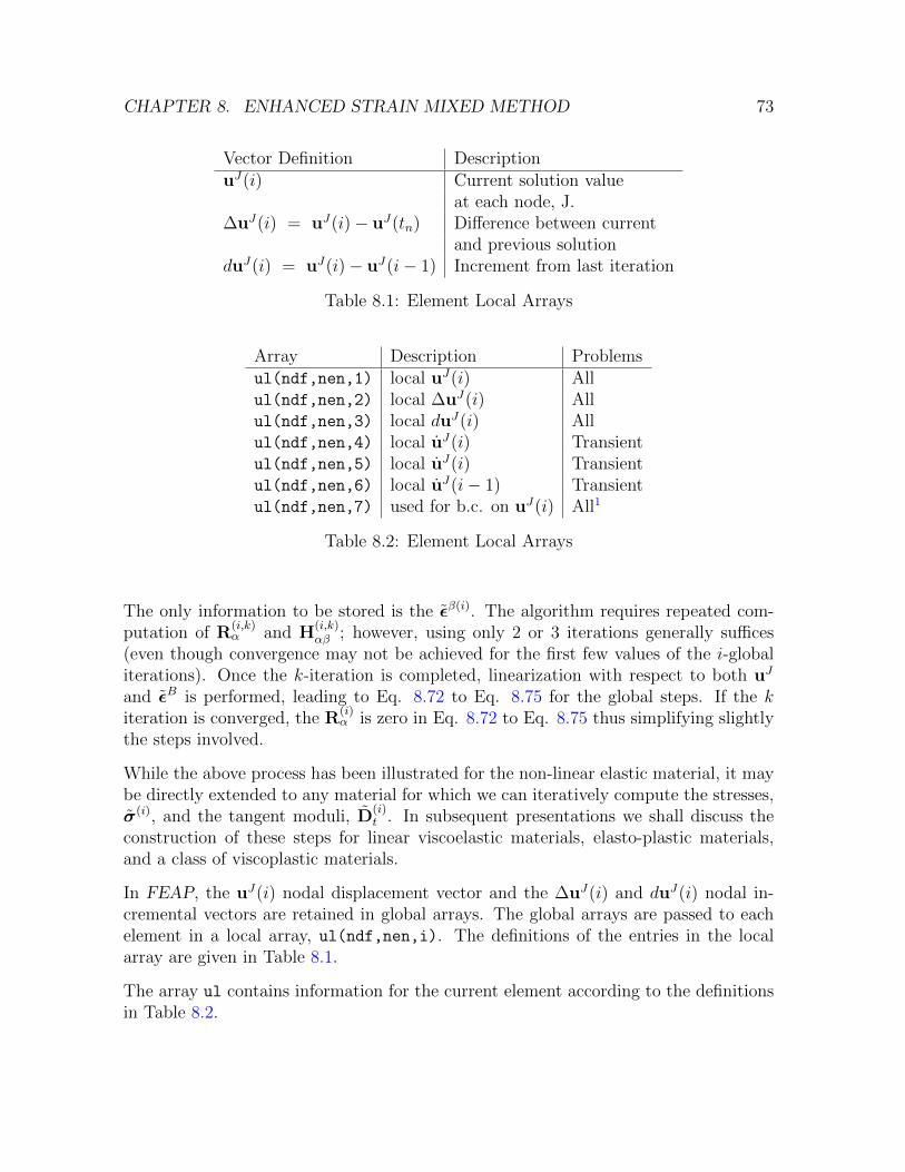
CHAPTER 8. ENHANCED STRAIN MIXED METHOD 73
Vector Definition DescriptionuJ(i) Current solution value
at each node, J.∆uJ(i) = uJ(i)− uJ(tn) Difference between current
and previous solutionduJ(i) = uJ(i)− uJ(i− 1) Increment from last iteration
Table 8.1: Element Local Arrays
Array Description Problemsul(ndf,nen,1) local uJ(i) Allul(ndf,nen,2) local ∆uJ(i) Allul(ndf,nen,3) local duJ(i) Allul(ndf,nen,4) local uJ(i) Transientul(ndf,nen,5) local uJ(i) Transientul(ndf,nen,6) local uJ(i− 1) Transientul(ndf,nen,7) used for b.c. on uJ(i) All1
Table 8.2: Element Local Arrays
The only information to be stored is the εβ(i). The algorithm requires repeated com-putation of R
(i,k)α and H
(i,k)αβ ; however, using only 2 or 3 iterations generally suffices
(even though convergence may not be achieved for the first few values of the i-globaliterations). Once the k-iteration is completed, linearization with respect to both uJ
and εB is performed, leading to Eq. 8.72 to Eq. 8.75 for the global steps. If the kiteration is converged, the R
(i)α is zero in Eq. 8.72 to Eq. 8.75 thus simplifying slightly
the steps involved.
While the above process has been illustrated for the non-linear elastic material, it maybe directly extended to any material for which we can iteratively compute the stresses,σ(i), and the tangent moduli, D
(i)t . In subsequent presentations we shall discuss the
construction of these steps for linear viscoelastic materials, elasto-plastic materials,and a class of viscoplastic materials.
In FEAP, the uJ(i) nodal displacement vector and the ∆uJ(i) and duJ(i) nodal in-cremental vectors are retained in global arrays. The global arrays are passed to eachelement in a local array, ul(ndf,nen,i). The definitions of the entries in the localarray are given in Table 8.1.
The array ul contains information for the current element according to the definitionsin Table 8.2.
Chapter 9
Linear Viscoelasticity
9.1 Isotropic Model
The representation of a constitutive equation for linear viscoelasticity may be in theform of either a differential equation or an integral equation form. In the discussionto be presented here we assume the material is linear and isotropic. Accordingly, inmatrix form the stress and strain may be split as
σ = s + m p (9.1)
and
ε = e +1
3m θ (9.2)
where σ is the Cauchy stress, s is the stress deviator, and p is the mean (pressure)stress defined in matrix form as
p =1
3mT σ (9.3)
ε is strain, e is the strain deviator, and θ is the volume change defined in matrix formas
θ = mT ε (9.4)
In the presentation given here we assume that the pressure-volume parts of the behaviorare governed by a linear elastic model
p = K θ (9.5)
where K is the bulk elastic modulus defined in terms of Young’s modulus and Poisson’sratio as
K =E
3 (1− 2 ν)(9.6)
74
CHAPTER 9. LINEAR VISCOELASTICITY 75
The deviatoric parts are assumed to satisfy a linear viscoelastic model.
Linear viscoelastic behavior may be stated in the form of differential equation modelsor in the form of integral equations. In the differential equation model the constitutiveequation may be written as
P (s) = 2GQ(e) (9.7)
where P and Q are differential operators expressed as
P = pm∂m
∂tm+ pm−1
∂m−1
∂tm−1+ · · · + p0 (9.8)
Q = qm∂m
∂tm+ qm−1
∂m−1
∂tm−1+ · · · + q0 (9.9)
and
G =E
2 (1 + ν)(9.10)
is identical to the elastic shear modulus. Alternatively, the operator may be written as
s = 2G (µ0e +N∑i=1
µi qi) (9.11)
qi +1
λiqi = e (9.12)
This form of the representation is equivalent to a generalized Maxwell model (a set ofMaxwell models in parallel). The set of first order differential equations may be inte-grated for specified strains, e. The integral for each term is given by the homogeneousdifferential equation solution, qih,
qih(t) = C exp−tλi
(9.13)
and variation of parameters on C to give
qi(t) =
∫ t
−∞exp−t− τ
λ1
e(τ) dτ (9.14)
An advantage to the differential equation form is that it may be easily extended toinclude aging effects by making the parameters time dependent.
An alternative to the linear viscoelastic model in differential form is to use an integralequation form. The integral form equivalent to the above is expressed in terms of therelaxation modulus function. The relaxation modulus function is defined in terms of anidealized experiment in which, at time labeled zero (t = 0), a specimen is subjected toa constant strain, e0, and the stress response, s(t), is measured. For a linear material
CHAPTER 9. LINEAR VISCOELASTICITY 76
a unique relation is obtained which is independent of the magnitude of the appliedstrain. This relation may be written as
s(t) = 2G(t) e0 (9.15)
where G(t) is defined as the shear relaxation modulus function. Using linearity andsuperposition for an arbitrary state of strain yields an integral equation specified as
s(t) =
∫ t
−∞G(t− τ) e(τ) dτ (9.16)
It is noted that the above form is a generalization of the Maxwell material. Indeed theintegral equation form may be defined as a generalized Maxwell model by assumingthe shear relaxation modulus function in the Prony series form
G(t) = G0 +N∑i=1
Gi exp−tλi
(9.17)
or the alternate form
G(t) = G (µ0 +N∑i=1
µi exp−tλi
) (9.18)
where
µ0 +N∑i=1
µi = 1 (9.19)
With this form the integral equation form is identical to the differential equation modelfor the generalized Maxwell material. In the subsequent discussion we will consider thegeneralized Maxwell material and let N be 1 (i.e., the standard linear solid). Theaddition of more terms may be easily accommodated based upon the one term repre-sentation. Accordingly,
G(t) = G (µ0 + µ1 exp−tλ1
) (9.20)
whereµ0 + µ1 = 1 (9.21)
In applications involving a linear viscoelastic model, it is usually assumed that thematerial is undisturbed until a time identified as zero. At time zero a strain may besuddenly applied and then varied over subsequent time. The integral representationfor the the model may be simplified by dividing the integral into∫ t
−∞(·) dτ =
∫ 0−
−∞(·) dτ +
∫ 0+
0−(·) dτ +
∫ t
0+(·) dτ (9.22)
CHAPTER 9. LINEAR VISCOELASTICITY 77
The first term is zero, the second term includes a jump term associated with e0 attime zero, and the last term covers the subsequent history of strain. The result of thisseparation when applied to Eq. 9.16 gives
s(t) = 2G(t) e0 + 2
∫ t
0
G(t− τ) e(τ) dτ (9.23)
where subsequently the 0 limit on the integral is understood as 0+.
Substitution of Eq. 9.20 into Eq. 9.23 gives
s(t) = 2G [µ0 e(t) + µ1 exp−tλ1
(e0 +
∫ t
0
expt
λ1
e(τ) dτ)] (9.24)
It remains to evaluate the integral. Accordingly, we divide the integral as∫ t
0
(·) dτ =
∫ tn
0
(·) dτ +
∫ t
tn
(·) dτ (9.25)
If we define the integral as
i1(t) =
∫ t
0
expτ
λ1
e(τ) dτ (9.26)
the above separation gives
i1(t) = i1(tn) +
∫ t
tn
expτ
λ1
e(τ) dτ (9.27)
Including the negative exponential multiplier term gives
h1 = exp−tλ1
i1 (9.28)
and then
h1(t) = exp−∆t
λ1
h1n + ∆h (9.29)
where
∆h = exp−tλ1
∫ t
tn
expτ
λ1
e(τ) dτ (9.30)
The strain rate is now approximated as constant over each time increment tn to t, thus
e(τ) ≈ e(t)− en∆t
; tn ≤ τ ≤ t (9.31)
where en denotes the value of the strain at time tn and ∆t denotes the time incrementt − tn. A numerical approximation to ∆h may be employed and one proposal uses amidpoint (one-point) approximation for the integral as [8]
∆h = exp−∆t
2λ1
(e− en) (9.32)
CHAPTER 9. LINEAR VISCOELASTICITY 78
The recursion then becomes∫ t
tn
expτ
λ1
dτ ≈ ∆t exptn+ 1
2
λ1
(9.33)
where tn+ 12
denotes the time 12(tn + t). Thus, the recurrsion is now given in the form
h1(t) = exp−tλ1
i1(t) = exp−∆t
λ1
[h1n + exp
∆t
2λ1
(e − en)] (9.34)
and simplifies to
h1(t) = exp−∆t
2λ1
[exp−∆t
2λ1
h1n + (e − en)] (9.35)
This form requires only one evaluation of an exponential term. Furthermore, a zerovalue of the time step produces a correct answer, as well as, a very large value of thetime step producing a zero value. Thus, the form is doubly asymptotically accurate.The use of finite difference approximations on the differential equation form directlydoes not produce this property.
While the above form is easy to evaluate it has problems when the size of the timestep is changed. Thus, a more stable form is used in FEAP where the integral over thetime step is evaluated in closed form [23]. The result gives
∆h =λ1
∆t
(1 − exp
−∆t
λ1
)(e− en) (9.36)
This approximation produces a singular ratio for zero time steps; however, the limitvalue is well behaved at a unit value. For very small time steps a series expansion maybe used to yield accurate values. This form gives a recursion which is stable for smalland large time steps and gives smooth transitions under variable time steps. It mayalso be extended for use with thermorheologically simple materials.
The constitutive equation now has the simple form
s(t) = 2G [µ0 e(t) + µ1 h1(t)] (9.37)
The inclusion of more terms in the series reduces to evaluation of additional hi(t)integral recursions. The required storage is increased by a need to preserve the hi foreach quadrature point in the problem and each term in the series.
The implementation of the viscoelastic model into a Newton solution process requiresthe computation of the tangent tensor. Accordingly, we need to compute
∂s
∂ε=
∂s
∂e
∂e
∂ε=
∂s
∂eIdev (9.38)
CHAPTER 9. LINEAR VISCOELASTICITY 79
where Idev is the deviatoric operator identified previously. The partial derivative withrespect to the deviatoric stress is given by
∂s
∂e= 2G [µ0 I + µ1
∂h1
∂e] (9.39)
If we let∆h1 = ∆h1(∆t) (e − en) (9.40)
the derivative of the last term in Eq. 9.39 becomes
∂h1
∂e= ∆h1(∆t), I (9.41)
Thus, the tangent tensor is given by
∂s
∂ε= 2G [µ0 + µ1 ∆h1(∆t)] Idev (9.42)
The only modification from a linear elastic material is the substitution of the factor
Gvisc = G [µ0 + µ1 ∆h1(∆t)] (9.43)
for the elastic shear modulus. Again we note that for zero ∆t the full elastic modulusis recovered, whereas for very large increments the equilibrium modulus µG0 is used.The above formulation is incorporated into the subroutine viscoe. Note the simplicityof the additional coding needed to include the linear viscoelastic formulation. Sincethe material is linear, use of the consistently derived tangent modulus terms leads toconvergence in one iteration (the second iteration produces a zero residual).
Chapter 10
Plasticity Type Formulations
10.1 Plasticity Constitutive Equations
The constitutive equations for a material which behaves according to a plasticity typeformulation for deformation states which exceed the elastic limit may be expressed byassuming that the strains are decomposed according to
ε = εe + εp (10.1)
where εe are the elastic strains and εp are the inelastic strains. If the material is non-linear hyper-elastic we may deduce the stress from the expression for the elastic strainenergy as
σ =∂W
∂ε
∣∣∣∣εe
(10.2)
where W is the strain energy density and is expressed as a function of the elasticstrains and σ and εe are stress and strain energy conjugates. For a linear hyper-elasticmaterial the stress to elastic strain relation is given by
σ = D εe = D (ε − εp − ε0) (10.3)
In the following discussion we limit our comments to linear elastic materials and alsoset ε0 zero. The inelastic component of the strain rate is related to the gradient of aloading function with respect to stress. Accordingly,
εp = γ∂f
∂σ(10.4)
where f is a loading function and γ is a scalar rate term called the plastic consistencyparameter. The plastic consistency parameter, γ, is zero for elastic behavior and pos-itive for plastic behavior. A back stress is defined as α which is related to the plastic
80
CHAPTER 10. PLASTICITY TYPE FORMULATIONS 81
strain rate through
α =2
3Hkin ε
p =2
3Hkin γ
∂f
∂σ(10.5)
where Hkin is a kinematic hardening modulus. The yield surface is defined in an as-sociative manner, using the same function as the loading function, and is expressedas
f(σ,α, ep) = F (Σ) − Y (ep) (10.6)
where the stress and back stress appear in the form
Σ = σ − α (10.7)
andY (ep) = Y0 + Hiso e
p (10.8)
is a function which measures the size of the current yield surface. Commonly, Y0 isrelated to σy, the yield stress in uniaxial tension. The isotropic hardening behavior ofthe material is included in Y through an effective or accumulated plastic strain definedby
ep =
∫ t
0
(2
3εp · εp
) 12
dτ (10.9)
In Eq. 10.8 Hiso is an isotropic hardening modulus. In the present study both theisotropic and the kinematic hardening moduli will be assumed as constants. Using thedefinition of the plastic strain rate the effective plastic strain may also be written as
ep =
∫ t
0
γ
(2
3
∂f
∂σ· ∂f∂σ
) 12
dt (10.10)
thus it is evident that ep is dependent on the integral of γ and the particular load-ing/yield function used to describe the material.
Generally, the model is completed by describing a scalar function, g, which describesthe limit behavior of the model. Different limit equations may be written for rateindependent plasticity, rate dependent plasticity, and generalized plasticity models.The simplest relation is for classical, associative, rate independent plasticity where
g = f(σ,α, ep) ≤ 0 (10.11)
is used. Later alternative forms will be introduced to represent other types of materialbehavior.
CHAPTER 10. PLASTICITY TYPE FORMULATIONS 82
10.2 Solution Algorithm for the Constitutive Equa-
tions
The solution of the above set of equations may be effected numerically using a varietyof algorithms. A very effective method to integrate plasticity equations is the operatorsplit method with a return map concept[17, 18, 3, 4] the algorithm may be extended toinclude a variety of modeling concepts for the limit behavior; however, for the presentwe restrict our attention to plasticity as defined by Eq. 10.11 above. Accordingly, adiscrete solution at time tn is defined in terms of the state σn, αn, εpn, and epn. Thesolution is then advanced to time tn+1 by specifying the strain, εn+1.
To initiate the solution at tn+1 a trial state is computed assuming the step is entirelyelastic. Recall that a step is elastic when γ is zero. This implies that there will be nochange to εp, α, or ep during an elastic increment. The step is initiated by taking thetrial values for plastic quantities
εpTRn+1 = εpn (10.12)
αTRn+1 = αn (10.13)
epTRn+1 = epn (10.14)
andγTRn+1 = 0 (10.15)
Thus for linear elasticityσTRn+1 = D (εn+1 − εpTRn+1) (10.16)
The trial stress given by Eq. 10.16 is checked in Eq. 10.6 and Eq. 10.11 to determineif the step is elastic or whether inelastic terms should be active. If the state at tn+1
is elastic the stresses (as well as other state variables) are set equal to the trial value;otherwise, a correction is required to include the inelastic terms.
For an inelastic step the stresses must satisfy (1.2) for the time tn+1 which requiresthe rate equations for εp and α to be integrated over the time increment. Accordingly,integrating non-linear terms using a backward Euler implicit method between tn andtn+1, the plastic strain is given by
εpn+1 = εpn + λn+1∂f
∂σ
∣∣∣∣n+1
(10.17)
and the back stress by
αpn+1 = αpn + Hkin λn+1∂f
∂σ
∣∣∣∣n+1
(10.18)
CHAPTER 10. PLASTICITY TYPE FORMULATIONS 83
where Hkin is a constant kinematic hardening parameter and the integral of the con-sistency parameter is given by
λn+1 = γn+1 − γn (10.19)
Similarly, evaluating Eq. 10.11 at tn+1 gives
gn+1 = fn+1 = 0 (10.20)
Finally, integration of Eq. 10.4 produces
epn+1 = epn + λn+1 (3
2
∂f
∂σ· ∂f∂σ
)12
∣∣∣∣n+1
(10.21)
The set of equations Eqs. 10.3, 10.18 and 10.20 constitute a set of non-linear equationsin terms of the values of σn+1, αn+1 and λn+1 which must be solved for each stress pointand each time step of interest. A Newton method may be used to solve the equations.To simplify the notation the subscripts on n+ 1 are omitted. The iteration counter isshown as a superscript (j) and initial iterate values are taken as the trial stress andzero λ(0). The iterative solution is continued until the norm the residuals are withinacceptable tolerance values (e.g., normally, half machine precision relative to the initialiterate values are used since Newton’s method then guarantees that machine precisionis achieved if the next iteration is checked). Before proceeding with Newton’s methodwe note that the following relations hold
∂f
∂σ=
∂f
∂Σ
∂Σ
∂σ=
∂f
∂Σ(10.22)
and∂f
∂α=
∂f
∂Σ
∂Σ
∂α= − ∂f
∂Σ(10.23)
Thus, treating the equations Eq. 10.18 and Eq. 10.20 as residual equations, in theform
R(j)σ = ε − εpn − D−1 σ(j) − λ
∂f
∂Σ(10.24)
R(j)α = αn + Hkinλ
∂f
∂Σ− α(j) (10.25)
andR
(j)f = − f(σ(j),α(j), ep(j)) (10.26)
we may linearize the equations to obtain (note the iteration counter j is omitted in thecoefficient array for simplicity) C −λ ∂2f
∂Σ2∂∂λ
(λ ∂f∂Σ
)
−Hkinλ∂2f∂Σ2 (I + Hkinλ
∂2f∂Σ2 ) −Hkin
∂∂λ
(λ ∂f∂Σ
)∂f∂Σ
T − ∂f∂Σ
T −A
dσ(j+1)
dα(j+1)
dλ(j+1)
=
R(j)σ
T(j)α
R(j)f
(10.27)
CHAPTER 10. PLASTICITY TYPE FORMULATIONS 84
where
A =∂Y
∂ep∂ep
∂λ(10.28)
and
C = D−1 + λ∂2f
∂Σ2 (10.29)
The solutions to Eq. 10.27 are computed and added to obtain the next iterates. Ac-cordingly,
σ(j+1) = σ(j) + dσ(j+1) (10.30)
α(j+1) = α(j) + dα(j+1) (10.31)
andλ(j+1) = λ(j) + dλ(j+1) (10.32)
define the next iterates. The solution is terminated whenever the norms of the residualsare smaller than a selected small tolerance.
Once convergence is achieved for each stress point evaluation (i.e., to compute the stressat each Gauss point for a given strain), the stresses may be used in the finite elementto compute each element residual. In addition it is necessary to compute the tangentmoduli, Dt, for use in the element stiffness matrix (if one is used) for the next iterationon the momentum balance equation. That is we need to perform a new solution tosee if the strains we used to compute the stresses are correct. This is accomplished, asbefore, by solving ∑
e
KIJ uJ = FI +∑e
RI (10.33)
where KIJ and RI are the element stiffness and residual, respectively. The computationof the tangent moduli may be obtained by noting that the computation of the last stressincrement in the Newton solution of Eq. 10.27 may be written asdσ(j+1)
dα(j+1)
dλ(j+1)
=
C −λ ∂2f∂Σ2
∂∂λ
(λ ∂f∂Σ
)
− Hkin λ∂2f∂Σ2 (I + Hkin λ
∂2f∂Σ2 ) − Hkin
∂∂λ
(λ ∂f∂Σ
)∂f∂Σ
T − ∂f∂Σ
T −A
−1 R
(j)σ
T(j)α
R(j)f
(10.34)
At convergence for the given strain, ε, the residuals will vanish; however, if we nowconsider a linearization with respect to strain only Rσ contributes to the change. Thelinearization of the residuals with respect to an increment of strain yields
Rσ = dε ; Rα = 0 ; Rf = 0 (10.35)
Denoting the inverse matrix asD11 D12 D13
D21 D22 D23
D31 D32 D33
=
C −λ ∂2f∂Σ2
∂∂λ
(λ ∂f∂Σ
)
−Hkinλ∂f∂Σ
(I + Hkinλ∂2f∂Σ2 ) −Hkin
∂∂λ
(λ ∂f∂Σ
)∂f∂Σ
T − ∂f∂Σ
T −A
−1
(10.36)
CHAPTER 10. PLASTICITY TYPE FORMULATIONS 85
The final result for the linearization with respect to strain givesdσ(j+1)
dα(j+1)
dλ(j+1)
=
D11 dε
D21 dε
D31 dε
(10.37)
thus, the tangent moduli for the next momentum iteration is
Dt = D11 (10.38)
Except for giving the form of f this completes the specification of the general algorithm.Multiple yield surfaces may be included by modifying Eq. 10.4 to
εp =K∑k=1
γk∂fk∂σ
(10.39)
with each part of the yield surface described by a separate function
gk = fk(σ,α, ep) ≤ 0 (10.40)
An active condition for each surface is denoted when γk ≥ 0. Thus, usually only 1 or2 of the surfaces are active at any time.
As constitutive equations become complex the specification of the parameters is moredifficult. A systematic procedure for determining the parameters from experimentaldata is given by Ju, et. al.[13]. The method provides the best estimates for the param-eters and their sensitivities to errors or inconsistencies in the data.
10.3 Isotropic plasticity: J2 Model
As in previous developments, the strain is again split into deviatoric, e, and volumetric(spherical), θ, parts and expressed in matrix notation as
ε = e +1
3m θ (10.41)
whereθ = mT ε (10.42)
For our study on inelastic behavior, the decomposition into elastic and plastic partsmay now be expressed as
e = ee + ep (10.43)
andθ = θe + θp (10.44)
CHAPTER 10. PLASTICITY TYPE FORMULATIONS 86
The stress also is split into the deviatoric, s, and pressure (spherical) parts as
σ = s + m p (10.45)
where
p =1
3mT σ (10.46)
With the above splits the isotropic linear elastic constitutive equations are given by
p = K (θ − θp) (10.47)
ands = 2G (e − ep) (10.48)
In the developments below we restrict plasticity to the deviatoric part only. Thus θp
vanishes and the yield function can depend only on the deviatoric part of the stress.For isotropic materials the yield and loading function may be expressed in terms of theinvariants of stress and back stress. The invariants of s are denoted as J1, J2, and J3
and given byJ1 = mT s = 0 (10.49)
J2 =1
2sT s (10.50)
andJ3 = det (s) (10.51)
The simplest formulation is where the function depends only on J2. We write thismodel using √
2 J2 = (sT s)12 = ‖ s ‖ (10.52)
and including the back stress, the limit equation as
g = f(s,α, ep) = ‖ s − α ‖ − Y (ep) ≤ 0 (10.53)
where Y is the radius of the yield function which is related to the uniaxial yield stress,σy, through
Y (ep) =
√2
3(σy + Hiso e
p) (10.54)
and, thus, includes the effects of linear isotropic hardening. The back stress adjustedvalue Σ is given by
Σ = s − α (10.55)
A simple calculation shows that
∂f
∂σ=
∂f
∂sIdev ;
∂f
∂s=
∂f
∂Σ
∂Σ
∂s=
∂f
∂Σ;
∂f
∂α=
∂f
∂Σ
∂Σ
∂α= − ∂f
∂Σ(10.56)
CHAPTER 10. PLASTICITY TYPE FORMULATIONS 87
(where we recall that Idev = I − 13m mT ), and
∂f
∂Σ=
Σ
‖ Σ ‖= n =
∂f
∂σ(10.57)
Thus, the evolution of the back stress satisfies
α =2
3Hkinγ
∂f
∂σ=
2
3Hkinγ n (10.58)
Noting that at the initial state α is zero, we can conclude that the back stress evolvessuch that it is a purely deviatoric quantity. thus,
mT α = 0 (10.59)
With this fact we then have the following important properties
mT Σ = 0 ; mT n = 0 ; nT n = 1 (10.60)
Based upon the above all aspects of the J2 plasticity model are restricted to deviatoriccomponents only. Thus, our model is completed by giving the evolution equations forplastic strain and effective plastic strain in the form
ep = γ n (10.61)
ep =
∫ t
0
√2
3γ dτ (10.62)
The discrete form of the isotropic J2 model is given by the equations
pn+1 = K θn+1 (10.63)
sn+1 = 2G (en+1 − epn+1) (10.64)
epn+1 = epn + λn+1 nn+1 (10.65)
αn+1 = αn +2
3Hkinλn+1 nn+1 (10.66)
epn+1 = epn +
√2
3λn+1 (10.67)
gn+1 = ‖ Σn+1 ‖ − Yn+1 ≤ 0 (10.68)
Σn+1 = sn+1 − αn+1 (10.69)
and
Yn+1 =
√2
3(σy + Hiso e
pn+1) = Yn +
2
3Hiso λn+1 (10.70)
CHAPTER 10. PLASTICITY TYPE FORMULATIONS 88
The solution of the J2 model is straight forward and may be accomplished by solvingonly a scalar equation in λn+1. The solution is performed using a trial state basedupon the assumption that λTRn+1 is zero. Accordingly,
epTRn+1 = epn ; αTRn+1 = αn ; epTRn+1 = epn (10.71)
This yields the trial deviator stresses
sTRn+1 = 2G (en+1 − epTRn+1) = 2G (en+1 − epn) (10.72)
which may be used to check the limit equation, gn+1. If the limit equation is satisfiedthen the trial values define the solution at tn+1. If the trial values violate the limitequation, it is necessary to perform the second part of the algorithm. The secondpart of the algorithm solves the discrete rate equations using the trial values as initialconditions. Accordingly, using Eqs. 10.65, 10.71 and 10.72 in Eq. 10.64 gives
sn+1 = sTRn+1 − 2Gλn+1 nn+1 (10.73)
Next subtracting Eq. 10.66 from Eq. 10.73 gives
Σn+1 = sn+1 − αn+1 = sTRn+1 − αn − 2 (G +1
3Hkin)λn+1 nn+1 (10.74)
Noting that Σn+1 = ‖ Σn+1 ‖ nn+1 Eq. 10.74 gives also that sTRn+1 − αn is in thedirection nn+1, and may be written as the scalar equation[
‖ Σn+1 ‖ − ‖ ΣTRn+1 ‖ + 2 (G +
1
3Hkin)λn+1
]nn+1 = 0 (10.75)
that is, the coefficient must vanish to obtain a solution. In the above
ΣTRn+1 = sTRn+1 − αn (10.76)
Combining Eq. 10.75 with Eq. 10.68 and Eq. 10.70 yields the scalar equation,
‖ ΣTR ‖ − Yn = 2 [G +1
3(Hiso + Hkin)]λn+1 (10.77)
Once λn+1 is known it may be combined with the result
nn+1 = nTRn+1 =ΣTRn+1
‖ ΣTRn+1 ‖
(10.78)
to give the stress assn+1 = sTRn+1 − 2Gλn+1 nn+1 (10.79)
CHAPTER 10. PLASTICITY TYPE FORMULATIONS 89
as well as the plastic strain and the back stress. In practice λn+1 is reduced slightly tothat sn+1 is always slightly outside the limit yield condition. Accordingly, the solutionto Eq. 10.78 is perturbed as
λn+1 =‖ ΣTR
n+1 ‖ − Yn (1 + tol)
2 [G + 13
(Hiso + Hkin)](10.80)
where tol is a small value, say 10−8.
The solution of the problem, as shown above, does not require a linearization or aniteration process. If non-linear isotropic hardening is included or alternative forms forthe limit equation are employed, the equation equivalent to Eq. 10.77 will be nonlinearin λn+1 and a linearization and iteration process are required to obtain a solution.Similarly, if non-linear kinematic hardening is introduced the reduction to a scalarequation may also be complicated.
Once the converged value for λn+1 is known and the stress state determined, a checkon satisfaction of the momentum equation must be made. If the momentum equationis not satisfied for the current time, tn+1, another iteration is necessary to improvethe estimate for the state of strain, εn+1. If a Newton type solution method is used itis necessary to compute an appropriate tangent modulus matrix for each stress pointin the analysis. For the solution process developed here, this may be achieved byselecting as primary dependent variables the stress, sn+1, the back stress, αn+1, andthe consistency parameter, λn+1. Writing appropriate residual equations as
Rs = e − epn −1
2Gs − λn = 0 (10.81)
Rα = α − αn −2
3λHkin n = 0 (10.82)
and
Rf = Yn +2
3Hiso λ − ‖ Σ ‖ = 0 (10.83)
In the above we have deleted specific reference to the values at tn+1, to avoid addedcomplexity in the linearization performed below. It should be understood that λ de-notes the value of the solution in the tn+1 step, i.e., previously given as λn+1, and etc.for all the other variables. We note that for the current strain, e, the above equationsare satisfied; however, to proceed to the next iteration of the momentum equation weconsider a linearization of the above equations with respect to a change in the strainalso, which we denote by de. Accordingly, the linearization n becomes
∂n
∂Σ=
1
‖ Σ ‖(I − n nT ) =
1
‖ Σ ‖N (10.84)
CHAPTER 10. PLASTICITY TYPE FORMULATIONS 90
Using this result, the linearization of Eqs. 10.81 to 10.83 yields the set of equations1
2GI + λ
‖Σ‖ N − λ‖ΣTR‖ N n
− 2λHkin
3 ‖Σ‖ N I + 2λHkin
3 ‖Σ‖ N − 23Hkin n
nT −nT − 23Hiso
dsdαdλ
=
de00
(10.85)
The inverse to the coefficient matrix may be computed by first solving the first twoequation for ds and dα in terms of dλ and de, and then substituting the result into thethird equation to obtain a final expression for dλ in terms of de. This also permits thesubstitution of alternative limit equations without changing the solution to the firstpart. Accordingly, we consider[
12G
I+ λ‖Σ‖
N − λ‖Σ‖ N
− 2λHkin
3 ‖ΣTR‖ N I + 2λHkin
3 ‖Σ‖ N
] [dsdα
]=
[de − n dλ− 2
3Hkin n dλ
](10.86)
The solution to this equation is1[dsdα
]=
[2G (I − BN) BN
2GC N I − C N
] [de − n dλ− 2
3Hkin n dλ
](10.87)
where B and C are given by
B =2Gλ
‖ Σ ‖D=
2Gλ
‖ ΣTR ‖; C =
2Hkin λ
3 ‖ Σ ‖ D=
2Hkin λ
3 ‖ ΣTR ‖(10.88)
and where we have noted that
D = 1 + 2 (G +Hkin
3)
λ
‖ Σ ‖=‖ ΣTR ‖‖ Σ ‖
(10.89)
This result may be substituted into the third equation in Eq. 10.85 to obtain
2GnT de = 2 [G +1
3(Hiso + Hkin)] dλ (10.90)
Substituting this result back into the first of equation Eq. 10.87 yields the incrementalequation which yields the tangent modulus matrix for the algorithm. Thus, we obtain
ds = 2G [I − B (I − n nT ) − An nT ] de (10.91)
where
A =G
G + 13
(Hiso + Hkin)(10.92)
Finally, for the differential strains, dε, the tangent becomes
ds = 2G[Idev − B (Idev − n nT ) − An nT
]dε (10.93)
1See Appendix E for a discussion on the inverse of this type of matrix.
CHAPTER 10. PLASTICITY TYPE FORMULATIONS 91
10.4 Isotropic viscoplasticity: J2 model
The previous section presented the formulation and solution algorithm for a J2 classicalplasticity model. In this section we show how such a formulation may be easily extendedto include rate effects in the inelastic behavior. The model selected for exposition isclassical viscoplasticity as introduced by Prager for one-dimension and extended to fullthree-dimensional form by Perzyna[15].
For the viscoplastic model considered here, the only modification to the formulationis the replacement of the limit equation for g. Indeed, other models representing theproblems of generalized plasticity and generalized viscoplasticity can also be developedby such replacement. In viscoplasticity, the relationship for g becomes a constitutiveequation describing the evolution for the consistency parameter, γ. Accordingly, wewrite
g = Φ [f(s,α, ep)] − ζ γ ≤ 0 (10.94)
where the yield condition, f , still is given by
f(s,α, ep) = ‖ s − α ‖ − Y (ep) (10.95)
with Y the radius of the yield function which is related to a uniaxial yield stress, σy,through
Y (ep) =
√2
3(σy + Hiso e
p) (10.96)
and, thus, includes the effects of linear isotropic hardening. For viscoplasticity, Y andσy relate to the inelastic behavior in the limit as γ tends to zero (the rate independentlimit). For loading rates which are finite, the stress state may lie outside the yieldsurface. The function Φ together with the parameter ζ determine the rate dependencyof the model. Perzyna considers alternatives for representing Φ; however, here werestrict our attention to the simple case given by
Φ (f) =
(f
Y (0)
)m(10.97)
where m is a positive integer power. Other functional forms for Φ may be consideredwithout conceptual difficulty. All the other equations for the model remain as given inSection 10.3.
For trial stress values for which the yield function defined by Eq. 10.95 exceeds zero,the behavior is inelastic and the return map solution for the viscoplastic model is givenby Eqs. 10.63 to 10.67, 10.69 and 10.70. The formulation is completed by integrationof the constitutive equation Eq. 10.94 for the time interval tn to tn+1 (i.e., ∆t) usinga backward Euler evaluation of the integrals to obtain
∆tΦ [f (sn+1,αn+1, epn+1)] − ζ λn+1 = 0 (10.98)
CHAPTER 10. PLASTICITY TYPE FORMULATIONS 92
The discrete consistency parameter may be obtained by combining the scalar coeffi-cient from Eq. 10.75 with Eq. 10.98 to obtain a single nonlinear equation in λn+1.Accordingly, we obtain
∆tΦ
[‖ ΣTR ‖ − Yn − 2 (G + 1
3(Hiso + Hkin))λn+1
Y0
]− ζ λn+1 = 0 (10.99)
For the simple model used here for Φ, the above becomes
∆t
(‖ ΣTR ‖ − Yn − 2 [G + 1
3(Hiso + Hkin)]λn+1
Y0
)m
− ζ λn+1 = 0 (10.100)
In general, the above equation is nonlinear and must be solved numerically. For thecase where m = 1 the equation is linear and has the solution
λn+1 =∆t (‖ ΣTR
n+1 ‖ − Yn (1 + tol))
ζ Y0 + 2 ∆t [G + 13
(Hiso + Hkin)](10.101)
Comparing Eq. 10.101 to Eq. 10.80 we can observe that the limit solution for ζ zerois identical to the classical plasticity problem. The stress, back stress, plastic strain,and effective plastic strain are computed using the same expressions as for the classicalplasticity model. For nonzero ζ, the presence of ∆t in Eq. 10.101 implies a ratedependency, with results depending on time durations for applying and changing loadson the body. The extension to higher powers of m may be constructed using a Newtonsolution scheme to solve the non-linear scalar equation.
Chapter 11
Augmented LagrangianFormulations
11.1 Constraint Equations - Introduction
The solution of many problems requires imposition of constraints as part of the for-mulation. For example, if it is desired to solve the incompressible equations for linearelasticity it is necessary to impose the constraint
tr(ε) = mT ε = 0 (11.1)
Another type of constraint is to impose boundary conditions on a node, where we wishto impose the condition for node I that
uI = uI (11.2)
in which u denotes a specified value. This type of constraint can be made more generalby letting the degrees-of-freedom be associated with a rotated local coordinate system(e.g., a spherical coordinate frame) where now
u′I = TI uI = u′I (11.3)
in which TI is an orthogonal rotation matrix which transforms the degrees-of-freedomfrom the global Cartesian to the prime system. Many other conditions could be given;however, the above suffice for the present. The inclusion of the constraints into the finiteelement problem may be performed by several different approaches. For constraints ofthe type Eq. 11.2 it is easy to directly eliminate the variables associated with uI , as isdone in FEAP. On the other hand the inclusion of Eq. 11.1 or Eq. 11.3 presents moredifficulty to implement. Thus, an alternative method is needed to implement generaltypes of constraints. A common approach is to use penalty methods; however, these
93
CHAPTER 11. AUGMENTED LAGRANGIAN FORMULATIONS 94
are sensitive to the value of the penalty parameter selected. A better approach, whichis numerically superior, is to use an augmented Lagrangian approach. This method isan extension to the penalty method and uses values for the penalty parameter whichlead to a better conditioned numerical problem. In the sequel we first consider penaltymethods, based upon a mixed formulation. Subsequently, we show how to extend themixed penalty treatment to the augmented Lagrangian algorithm which is based on aniterative update procedure generally attributed to Uzawa [1].
11.2 Mixed Penalty Methods for Constraints
Consider a general constraint equation expressed as
g(u) = 0 (11.4)
which is to be imposed for some part of the domain, Ωc. The constraint may beincluded as part of the problem formulation by supplementing the variational problem,Π(u), with the term
Πc(u,λ) =
∫Ωc
λT g(u) dΩ (11.5)
Define the variations asuη = u + ηU (11.6)
andλη = λ + ηΛ (11.7)
The variation of the integral gives the added terms
dΠcη
dη
∣∣∣∣η=0
=
∫Ωc
ΛT g(u) dΩ +
∫Ωc
UT GT λ dΩ (11.8)
where
G =∂g
∂u(11.9)
The Euler equation for the first integral leads to the constraint equation.
g(u) = 0 (11.10)
for each point in Ωc, and the second equation leads to a term which is combined withthe variation of the original variational theorem to generate revised Euler equationsfor the problem.
In a finite element matrix setting we can approximate the λ in each element as
λ = Nλα(x)λα (11.11)
CHAPTER 11. AUGMENTED LAGRANGIAN FORMULATIONS 95
and use the usual isoparametric interpolations for u. Thus, Eq. 11.8 generates thematrix problem
G =dΠcη
dη
∣∣∣∣η=0
=[(Λα)T (UI)T
] [Pλα
PλI
](11.12)
where
Pλα =
∑e
∫Ωce
Nλα g(u) dΩ (11.13)
and
PλI =
∑e
∫Ωce
NI GT λ dΩ (11.14)
For non-linear constraint equations it is necessary to linearize this expression for com-bination with the remaining part of the problem. Performing the linearization leads tothe problem [
(Λα)T (UI)T] [ 0 Kλ
αJ
KλIβ Kλ
IJ
] [dλβ
duJ
](11.15)
where
KλIβ =
∑e
∫Ωce
NI GT Nλβ dΩ (11.16)
KλαJ =
∑e
∫Ωce
Nλα GNJ dΩ = (Kλ
Jα)T (11.17)
and
KλIJ =
∑e
∫Ωce
NI λT ∂2g
∂u∂uNJ dΩ =
∑e
∫Ωce
NI λT ∂G
∂uNJ dΩ (11.18)
The difficulty with the above formulation lies in the fact that there are no termsin Eq. 11.15 which are associated with the diagonals for the λ degrees-of-freedom.Moreover, if the constraints are linear there are no terms on the diagonals for any ofthe degrees-of-freedom. This greatly, complicates a solution process since for a directsolution the equations must be ordered to eliminate the displacement equations priorto the Lagrange multiplier equations. Furthermore, iterative methods are even moredifficult to consider. The deficiency associated with the diagonals for the Lagrangemultiplier equations may be removed by adding a regularization term to Eq. 11.5. Themodification to the variational term considered takes the form
Πc(u,λ) =
∫Ωc
λT g(u) dΩ −∫
Ωc
1
kλTλ dΩ (11.19)
where k is a penalty parameter introduced such that in the limit as k goes to infinitythe original problem is recovered.
dΠcη
dη
∣∣∣∣η=0
=
∫Ωc
ΛT (g(u) − 1
kλ) dΩ +
∫Ωc
UT GT λ dΩ (11.20)
CHAPTER 11. AUGMENTED LAGRANGIAN FORMULATIONS 96
The Euler equation for the first integral now gives the constraint equation.
g(u) − 1
kλ = 0 (11.21)
for each point in Ωc. It is evident that the solution converges to satisfy the constraintonly in the limit when k is infinity. The linearization of Eq. 11.20 gives the matrixproblem [
(Λα)T (UI)T] [Kλ
αβ KλαJ
KλIβ Kλ
IJ
] [dλβ
duJ
](11.22)
where
Kλαβ =
∑e
∫Ωce
Nλα
1
kINλ
β dΩ (11.23)
Many cases for constraints permit the elimination of the equations for λα at a locallevel. Thus, if a Newton solution scheme is employed the residual equations may bewritten as[
Rλα
RI(u) + RλI
]=
[−Pλ
α + Kλαβ λ
β
R(Iu
) − PλI
]−[−Kλ
αβ KλαJ
KλIβ KIJ + Kλ
IJ
] [dλβ
duJ
]=
[00
](11.24)
This gives the set of equations to solve for the increment as[−Kλ
αβ KλαJ
KλIβ KIJ + Kλ
IJ
] [dλβ
duJ
]=
[−Pλ
α + Kλαβ λ
β
RI(u) − PλI
](11.25)
Solving the first row of Eq. 11.25 gives
dλβ = (Kλαβ)−1
[Pλα + Kλ
αJ duJ]− λβ (11.26)
Since the residual equation for λβ is linear it may be solved to give
λβ =(Kλαβ
)−1Pλα (11.27)
and this simplifies Eq. 11.26 to
dλβ =(Kλαβ
)−1KλαJ du
J (11.28)
which when substituted into the second of Eq. 11.25 once again yields a displacementmodel for the problem which is expressed as
KIJ duJ = RI(u) − Pλ
I (11.29)
whereKIJ = KIJ + Kλ
IJ + KλIβ
(Kλαβ
)−1KλαJ (11.30)
CHAPTER 11. AUGMENTED LAGRANGIAN FORMULATIONS 97
The above solution process defines a perturbed Lagrangian form of the penalty solu-tion process. In order to yield a solution which provides an adequate satisfaction ofthe constraint equation, fairly large values for the penalty parameter should be used(generally on the order of about half machine precision, e.g., 106 or 107). The valuesused then yield stiffness modifications for the second term on the right hand side ofEq. 11.30 which are several orders larger than components appearing in the stiffness,KIJ . If the values are too large, ill conditioning for the solution to the linear equationswill result; if too small, the constraint may be violated by an unacceptable amount.Furthermore, iterative solutions become very difficult for these large penalty values.Consequently, an alternative approach is needed. In the next section, the augmentedLagrangian method is introduced as an alternative.
11.3 Augmented Lagrangian Method for Constraints
The augmented Lagrangian strategy presented is a simple modification to the perturbedLagrangian form which now becomes
Πc(u,λ,λA) =
∫Ωc
(λ + λA)T g(u) dΩ −∫
Ωc
1
kλTλ dΩ (11.31)
where λA is the augmented term. The variation to Eq. 11.31 gives
dΠcη
dη
∣∣∣∣η=0
=
∫Ωc
ΛT
(g(u) − 1
kλ
)dΩ +
∫Ωc
UT GT (λ + λA) dΩ (11.32)
+
∫Ωc
ΛTA g(u) dΩ (11.33)
The Euler equation for the variation of λ gives the equation
g(u) − 1
kλ = 0 (11.34)
which may be used to compute λ. The variation for λA gives the constraint equation
g(u) = 0 (11.35)
and, thus, the constraint equation is satisfied independently of the value of the penaltyparameter, k, and we also conclude that λ must vanish at the solution. Using, thesefacts we also note that the algorithm merely reduces to the original Lagrange multipliermethod, but with λA used as the multiplier. The method may be made computation-ally viable by making the determination of λA an iterative algorithm. The Uzawaalgorithm is the simplest algorithm which may be considered. In the Uzawa algorithmwe introduce an outer iteration loop for the augmentation. For each step in the analysiswe assume:
CHAPTER 11. AUGMENTED LAGRANGIAN FORMULATIONS 98
1. Let j be the augmentation iteration counter. For each time, tn+1, set j to zeroand take the initial value of the augmented multiplier as
λβ(j)A = λβA(tn) (11.36)
where the dependence on the n+1 step on the left side is implied. Let λβA(0) = 0.
2. Solve the non-linear problem[−Kλ
αβ KλαJ
KλIβ KIJ + Kλ
IJ
] [dλβ
duJ
]=
[−Pλ
α + Kλαβ λ
β
R(Iu
) − (PA)λI
]=
[0
RI(u) − (PA)λI
](11.37)
whereλβ =
(Kλαβ
)−1Pλα (11.38)
and
(PA)λI =∑e
∫Ωce
NI GT Nλβ (λβ + λ
β(j)A ) dΩ (11.39)
In the above the iteration aspects for the incremental problem are not shown.
3. After the iteration for the incremental problem converges update the augmentedparameters using
λβ(j+1)A = λ
β(j)A + λβ (11.40)
whereλβ =
(Kλαβ
)−1Pλα (11.41)
is computed using the converged solution from step 2.
4. Check convergence for the augmented step. If the constraint is satisfied to withina specified tolerance, or the change in the λβ is less than some tolerance timesλβ(j+1)A proceed to the next time and repeat steps 1 to 3.
If not converged increase the j counter and repeat steps 2 and 3.
To perform the above algorithm it is necessary for the penalty parameter k to be largeenough for the iteration to converge. All that is required is that the terms in the addedstiffness be somewhat larger than the original stiffness terms. The convergence rate forthe augmented iteration is generally linear, not quadratic as in a Newton solution. Thelarger k is made the more rapid the convergence. Thus, it is desirable for the value tobe at least one or two orders in magnitude larger than the conventional stiffness terms(as compared with the six or seven used in a penalty approach). Use of values withthis range in magnitudes leads to 3-6 augmented steps for most problems. The numberof non-linear iterations will decrease for the later augmented steps since the violationin the constraint is becoming less and less.
CHAPTER 11. AUGMENTED LAGRANGIAN FORMULATIONS 99
Using the above augmented Lagrangian approach to satisfy the incompressibility con-straint leads to a particularly simple update. For the constant pressure/volume elementthere is only one equation for each element. Thus the equations to be solved are scalar.For the enhanced element there is one equation at each Gauss point so it is also easy tomodify. For more complex situations, involving multi-point constraints, the situationis slightly more complex. Augmented approaches have been used to solve a varietyof problems in finite element methods. In some cases (for example, frictional contactproblems) it is possible to augment in a way which renders a problem which origi-nally has an un-symmetric tangent matrices to one which is symmetric. In general,the method is the one of current choice since, as a special case, it also includes anoption of penalty solution through the perturbed Lagrangian approach (merely omitall augmented steps!).
Chapter 12
Transient Analysis of Non-LinearProblems
12.1 Adding the transient terms
The variational equation for a quasi-static problem solved by the finite element methodis expressed as
dΠη
dη
∣∣∣∣η=0
=∑e
(UI)T[∫
Ωe
BTI σ dΩ −
∫Ωe
NI bv dΩ −∫
Γe
NI t dΓ
]= 0 (12.1)
where σ is computed for a displacement, mixed, or enhanced method as describedin previous chapters. In order to extend the variational equation to accommodatetransient analysis, the body force vector, bv, is replaced by
bv ← bv − ρ u (12.2)
in which u is the acceleration vector. With this replacement the variational equationbecomes
dΠη
dη
∣∣∣∣η=0
=∑e
(UI)T[∫
Ωe
BTI σ dΩ +
∫Ωe
NI ρ u dΩ −∫
Ωe
NI b dΩ
−∫
Γe
NI t dΓ
]= 0 (12.3)
which leads to the residual equation for each node
RI = FI −∑e
∫Ωe
BTI σ dΩ −
∑e
∫Ωe
NI ρ u dΩ (12.4)
100
CHAPTER 12. TRANSIENT ANALYSIS 101
The last term is the inertia contribution to the momentum equation. For continuumproblems the acceleration is computed from the isoparametric interpolations as
u = NJ(x) uJ(t) (12.5)
thus, the inertia term may be written as∑e
∫Ωe
NI ρ u dΩ = MIJ uJ (12.6)
where MIJ is the mass matrix for the problem. If we define
PI(σ) =∑e
∫Ωe
BI σ dΩ (12.7)
the residual equation becomes
RI = FI − PI(σ) − MIJ uJ (12.8)
or, by ignoring the nodal indices, in the total matrix form as
R = F − P(σ) − M u (12.9)
In general, the above equation is a non-linear set of ordinary differential equations.The practical solution of the equations is accomplished using a time marching scheme,as described in the next section.
12.2 Newmark Solution of Momentum Equations
In this section we illustrate the solution of Eq. 12.9 by a time marching process usingthe classical Newmark method of solution [14]. The Newmark method is a one-stepmethod which may be used to advance a solution from time tn to time tn+1. Themethod is self starting, consequently, given the initial conditions,
u(0) = d0 ; u(0) = v0 (12.10)
where d0 and v0 are the initial displacement and velocity vectors, the solution at thefirst increment may be determined. The Newmark method uses approximations to thedisplacements, velocities, and accelerations and these are given as:
un ≈ u(tn) (12.11)
vn ≈ u(tn) (12.12)
CHAPTER 12. TRANSIENT ANALYSIS 102
andan ≈ u(tn) (12.13)
The initial state is completed by solving the residual equation at time zero. Accordingly,
R0 = F0 − P(σ0) − M a0 = 0 (12.14)
which yields the solutiona0 = M−1 [F0 − P(σ0)] (12.15)
this is combined with the initial conditions
u0 = d0 ; v0 = v0 (12.16)
to give a complete state at time zero.
The Newmark formulas to advance a solution are given by
un+1 = un + ∆tvn + ∆t2[(1
2− β) an + β an+1
](12.17)
andvn+1 = vn + ∆t [(1 − γ) an + γ an+1] (12.18)
in which β and γ are numerical parameters which control the stability and numeri-cal dissipation, respectively. For γ = 1
2there is no numerical dissipation, whereas
for γ > 12
numerical dissipation is introduced. The values of β control primarilythe stability but also influence the form of the matrix problem. A β of zero leadsto a formulation which is called explicit, where for no damping, the solution for theacceleration, an+1, involves only the mass matrix. For a diagonal mass this solutionstep is very efficient; however, in general the method is only conditionally stable andvery small time steps are needed. For β non-zero, the method is implicit and a solu-tion step normally involves linearization of the momentum equation and an iterativesolution process based on Newton’s method. The advantage of implicit solutions isimproved stability, where quite large time steps may usually be taken. For example,for β = 0.25, the method for linear problems is unconditionally stable. This methodis commonly called trapezoidal rule or constant average acceleration. Values of β lessthan 0.25 should not be used since they are only conditionally stable with allowabletime steps not much larger than the explicit scheme.
The advancement of a solution from one step to the next is completed by combining Eq.12.17 and Eq. 12.18 with the momentum equation written at time tn+1. Accordingly,
Rn+1 = Fn+1 − P(σn+1) − M an+1 = 0 (12.19)
In order to advance the solution to the next time it is necessary to recast the problem inan iterative form. This involves selecting appropriate values for the variables to initiate
CHAPTER 12. TRANSIENT ANALYSIS 103
the step, linearization of the equations, solution of the linearized equations, and updat-ing of the variables. Since the Newmark formulas are linear and have scalar coefficientsthey may be directly used in the momentum equation to reduce the primary unknownsto a single vector. This vector may be the displacements, un+1, the velocities, vn+1,or the accelerations, an+1. For the explicit case the only viable choice is accelerations.In the sequel we will address the implicit case and use the displacements, un+1, as theprimary unknowns. For an implicit solution it is best to select the initial value for theiterate as
u(0)n+1 = un (12.20)
Any other choice may perturb the displacements in such a way to cause false inelasticvalues, especially near boundaries, which impede convergence of the Newton method.With the choice Eq. 12.20, the values of the initial state which satisfy the Newmarkformulas are given by
v(0)n+1 =
(1 − γ
β
)vn + ∆t
(1− γ
2 β
)an (12.21)
and
a(0)n+1 = − 1
β∆tvn +
(1− 1
2 β
)an (12.22)
Linearizing the Newmark formulas leads to the results
du(i+1)n+1 = β∆t2 da
(i+1)n+1 (12.23)
anddv
(i+1)n+1 = γ∆t da
(i+1)n+1 (12.24)
Thus the appropriate update formulas (which also satisfy the Newmark formulas) aregiven by
u(i+1)n+1 = u
(i)n+1 + du
(i+1)n+1 (12.25)
v(i+1)n+1 = v
(i)n+1 +
γ
β∆tdu
(i+1)n+1 (12.26)
and
a(i+1)n+1 = a
(i)n+1 +
1
β∆t2du
(i+1)n+1 (12.27)
The linearization of the momentum equation leads to
K?(i)t du
(i+1)n+1 = R
(i)n+1 (12.28)
where
K?(i)t = −
[∂R
∂u+
∂R
∂v
∂v
∂u+
∂R
∂a
∂a
∂u
](12.29)
or
K?(i)t = Kt +
γ
β∆tCt +
1
β∆t2M (12.30)
In Eq. 12.30, Kt is the tangent stiffness matrix as computed for the quasi-staticproblem, Ct is a tangent damping matrix, and M is the mass matrix introduced above.
CHAPTER 12. TRANSIENT ANALYSIS 104
12.3 Hilber-Hughes-Taylor (HHT) Algorithm
The Newmark algorithm given in the previous section can be altered by consideringthe residual for the momentum equation to be given by1
Rn+α = Fn+1 − P(un+α,vn+α) − M an+1 = 0 (12.31)
where the displacement at the intermediate point is given by2
un+α = (1− α) un + αun+1 (12.32)
and the velocity by
vn+α = (1− α) vn + αvn+1 (12.33)
In the above tn+α = (1 − α)tn + αtn+1. This algorithm is called the Hilber-Hughes-Taylor α-method or, for short, the HHT-method [9] and has been analyzed extensivelyfor stability and dissipative properties by Hughes [12]. To reduce the properties to asingle parameter, the relations,
β =(2− α)2
4(12.34)
and
γ =3
2− α (12.35)
are employed.
Linearization of 12.31 gives the tangent matrix
K? =1
β∆t2M +
αγ
β∆tC + αK (12.36)
for use in the Newton method
K? dun+1 = Rn+α (12.37)
1Note that the definition of α is different than in the original paper [9].2Note that the definition of α is different than in Hilber et al.[9].
Chapter 13
Finite Deformation Formulations:Elasticity
13.1 Kinematics and Deformation
The basic equations for solid mechanics may be found in standard references on thesubject (e.g., see Chadwick[2] or Gurtin[7]). Solution by finite element methods isconsidered by Crisfield in [3], by Curnier in [5], and by Zienkiewicz and Taylor in [27]..Here only a summary of the basic equations is presented. A body B has materialpoints whose positions are given by the vector X in a fixed reference configuration1,Ω0, in a three dimensional space. In Cartesian coordinates the position vector may bedescribed in terms of its components as:
X = XA EA ; A = 1, 3 (13.1)
where EA are unit base vectors. After the body is loaded each material point isdescribed by its position vector, x, in the current configuration, Ω. The positionvector in the current configuration may be given in terms of its components as
x = xa ea ; a = 1, 3 (13.2)
where ea are unit base vectors for the current time. In our discussion, common originsand directions are used for the reference and current coordinates. The position vectorat the current time is related to the reference configuration position vector through themapping
x = φ(X, t) (13.3)
1As much as possible we adopt the notation that upper case letters refer to quantities defined inthe reference configuration and lower case letters to quantities defined in the current configuration.Exceptions occur when quantities are related to both the reference and current configurations.
105
CHAPTER 13. FINITE DEFORMATION 106
When common origins and directions for the coordinate frames are used, a displacementvector, u, may be introduced as the change between the two frames. Accordingly,
x = 1 X + u (13.4)
is used. In the above 1 is a rank two shifter tensor between the two coordinate frames,and is given by
1 = δaAea ETA ; a, A = 1, 3 (13.5)
where δaA is a Kronecker delta quantity such that
δaA =
1 if a = A0 if a 6= A
(13.6)
In component form we then have
xa = δaAXA + ua (13.7)
A fundamental measure of deformation is described by the deformation gradient relativeto X given by
F =∂φ
∂X(13.8)
subject to the constraintJ = detF > 0 (13.9)
to ensure that material volume elements remain positive. The determinant of thedeformation gradient maps a volume element in the reference configuration into one inthe reference configuration, that is
dv = detF dV = J dV (13.10)
where dV is a volume element in the reference configuration and dv its correspondingform in the current configuration.
The deformation gradient relates the current configuration to the reference configura-tion, consequently it has components defined as
F = FaA ea ETA (13.11)
The deformation gradient may be expressed in terms of the displacement as
F = 1 +∂u
∂X(13.12)
Using F directly complicates the development of constitutive equations and it is com-mon to introduce deformation measures which are related completely to either the
CHAPTER 13. FINITE DEFORMATION 107
reference or the current configurations. Accordingly, for the reference configuration,the right Cauchy-Green deformation tensor, C, is introduced as
C = FT F (13.13)
Alternatively the Green strain tensor, E (do not confuse with the base vectors), isintroduced as
E =1
2(C − 10) (13.14)
where 10 is the rank two identity tensor with respect to the reference configuration andis given by
10 = δAB EA ETB (13.15)
and δAB is a Kronecker delta for the reference configuration. The Green strain may beexpressed in terms of the displacements as
E =1
2
[1T
∂u
∂X+ (
∂u
∂X)T 1 + (
∂u
∂X)T
∂u
∂X
](13.16)
Defining the displacement vector for the reference configuration as
U = 1 u (13.17)
with componentsUA = δaA ua (13.18)
the components of the Green strain may be written in the familiar form
EIJ =1
2
(∂UI∂XJ
+∂UJ∂XI
+∂UK∂XI
∂UK∂XJ
)(13.19)
In the current configuration a common deformation measure is the left Cauchy-Greendeformation tensor, b, expressed as
b = F FT (13.20)
The Almansi strain tensor, e, may be expressed in terms of b as
e =1
2
(1t − b−1
)(13.21)
where 1t is the rank two identity tensor with respect to the current configuration andis given by
1t = δab ea eTb (13.22)
and δab is a Kronecker delta for the current configuration.
CHAPTER 13. FINITE DEFORMATION 108
13.2 Stress and Traction Measures
Stress measures the amount of force per unit of area. In finite deformation problemscare must be taken to describe the configuration to which stress is measured. TheCauchy stress, σ, and the Kirchhoff stress, τ , are measures defined with respect to thecurrent configuration. They are related through the determinant of the deformationgradient as
τ = τab ea eTb = J σ = J σab ea eTb (13.23)
The second Piola-Kirchhoff stress, S, is a stress measure with respect to the referenceconfiguration and has components
S = SAB EA ETB (13.24)
The second Piola-Kirchhoff stress is related to the Kirchhoff stress through
τ = F S FT (13.25)
Finally, the first Piola-Kirchhoff stress, P, is related to S through
P = F S = PaA ea ETA (13.26)
which givesτ = P FT (13.27)
For the current configuration traction is given by
t = σT n (13.28)
where n is an unit outward pointing normal to a surface defined in the current configu-ration. This form of the traction may be related to reference surface quantity throughforce relations defined as
t ds = t0 dS (13.29)
where ds and dS are surface elements in the current and reference configurations,respectively, and t0 is traction on the reference configuration. Note that the directionof the traction component is preserved during the transformation and, thus, remainsrelated to the current configuration forces. The reference configuration traction isdeduced from the first Piola-Kirchhoff stress through
t0 = P N (13.30)
where N is an unit outward pointing normal to the reference surface. Using the defi-nition for traction and stresses we obtain
FT n ds = J N dS (13.31)
and
ds = J[N ·
(C−1 N
)] 1
2dS (13.32)
to relate changes in the surface area and transformation of the normals.
CHAPTER 13. FINITE DEFORMATION 109
13.3 Balance of Momentum
The balance of momentum for a solid body consists of two parts: balance of linearmomentum; and balance of angular momentum. The balance of linear momentum maybe expressed by integrating the surface and body loads over the body. Accordingly, fora body force per unit mass, bm the resultant force, R, acting on a body is given by∫
Ω
ρbm dv +
∫∂Ω
t ds = R (13.33)
where ρ is the mass density per unit volume and ∂Ω is the surface area of the body,both for the current configuration. The mass density in the current configuration isrelated to the reference configuration mass density, ρ0, through
ρ0 = J ρ (13.34)
The total linear momentum of the body is given by
p =
∫Ω
ρv dv (13.35)
The balance of linear momentum describes the translational equilibrium of a body (orany part of a body) and is obtained by equating the resultant force, R, to the rate ofchange of the body momentum, p. Accordingly,∫
Ω
ρbm dv +
∫∂Ω
tds =
∫Ω
ρ v dv (13.36)
Introducing the relationship between traction and stress and using the divergence prin-cipal leads to the balance of linear momentum relation∫
Ω
[divσ + ρ (bm − v)] dv = 0 (13.37)
where div is the divergence with respect to the current configuration, that is,
divσ =∂σab∂xa
eb (13.38)
Since the above result must hold for any part of a body a local form for balance oflinear momentum may be deduced as
divσ + ρbm = ρ v (13.39)
This relation is also called the local equilibrium equation for a body.
CHAPTER 13. FINITE DEFORMATION 110
Similar relations may be constructed for the balance of angular momentum and leadto the requirement
σ = σT (13.40)
that is, the Cauchy stress tensor is symmetric and, thus, has only six independentcomponents.
The balance of momentum may also be written for the reference configuration usingresults deduced above. Accordingly, we may write the integrals with respect to thereference body as ∫
Ω0
ρ0 bm dV +
∫∂Ω0
t0 dS =
∫Ω0
ρ0 v dV (13.41)
where the definitions for rho, σ and n ds in terms of reference configuration quantitieshave been used. Using the divergence principle on the traction term leads to the result∫
Ω0
[DivP + ρ0 (bm − v)] dV = 0 (13.42)
which has the local formDivP + ρ0 bm = ρ0 v (13.43)
In these relations Div is the divergence with respect to the reference configurationcoordinates
DivP =∂PaA∂XA
ea (13.44)
We also note that the symmetry of the Cauchy stress tensor, σ, leads to the corre-sponding requirement on P
F PT = P FT (13.45)
and subsequently to the symmetry of the second Piola-Kirchhoff stress tensor
S = ST (13.46)
13.4 Boundary Conditions
The basic boundary conditions for a solid region consist of two types: displacementboundary conditions and traction boundary conditions.
Boundary conditions are defined on each part of the boundary for which a componentor components of a vector may be specified without solution of any auxiliary problem.The conditions are usually given in terms of their components with respect to a localcoordinate system defined by the orthogonal basis, e′a, a = 1, 2, 3. At each point onthe boundary one (and only one) boundary condition must be specified for all three
CHAPTER 13. FINITE DEFORMATION 111
directions of the basis e′a. Generally, these conditions may be a mixture of displacementand traction boundary conditions.
For displacement boundary conditions, components of the position vector, x, may beexpressed with respect to the basis as
x = x′a e′a (13.47)
Boundary conditions may now be given for each component by requiring2
x′a = x′a (13.48)
for each point on the displacement boundary, ∂Ωu. The boundary condition may alsobe expressed in terms of components of the displacement vector, u. Accordingly,
u = x − 1 X = u′a e′a (13.49)
define components of the displacement with respect to the prime coordinates. Thus,boundary conditions may now be given for each displacement component by requiring
u′a = u′a (13.50)
In general, the boundary condition is non-linear unless points in the reference config-uration can be identified easily (such as fixed points).
The second type of boundary condition is a traction boundary condition. Using theorthogonal basis described above, the traction vector t may be written as
t = t′a e′a (13.51)
Traction boundary conditions may be given for each component by requiring
t′a = t′a (13.52)
for each point on the boundary, ∂Ωt.
13.5 Initial Conditions
Initial conditions describe the state of a body at the start of an analysis. The conditionsdescribe the initial kinematic state with respect to the reference configuration usedto define the body and the initial state of stress in this position. In addition, forconstitutive equations the initial values for internal variables which evolve in timemust be given.
2A specified quantity is indicated by a superposed bar, (·).
CHAPTER 13. FINITE DEFORMATION 112
The initial conditions for the kinematic state consist of specifying the position andvelocity at time zero. Accordingly,
x(0) = φ(X, 0) = d0(X) (13.53)
andv(0) = φ(X, 0) = v0(X) (13.54)
are specified at each point in the body.
The initial conditions for stresses are specified as
σ(0) = σ0 (13.55)
at each point in the body.
13.6 Material Constitution - Finite Elasticity
The equations are completed by specifying a material constitution. As an example, weconsider a finite deformation form for hyperelasticity. Thus, we postulate the existenceof a strain energy density function, W , from which stresses are computed by taking aderivative with respect to a deformation measure. For a strain energy density expressedin terms of the right Cauchy-Green deformation tensor, C, the second Piola-Kirchhoffstress tensor is computed as
S = 2∂ W
∂C(13.56)
For an isotropic material the strain energy density depends only on the three invariantsof the deformation. Here we consider the three invariants as
IC = trC = CKK (13.57)
IIC =1
2(I2C − trC2) =
1
2(CKK CLL − CKLCLK) (13.58)
andIIIC = detC = J2 (13.59)
and write the strain energy density as
W (C) = W (IC , IIC , J) (13.60)
We select J instead of IIIC as the measure of the volume change. Thus, the stress iscomputed as
S = 2∂ W
∂ IC
∂ IC∂C
+ 2∂ W
∂ IIC
∂ IIC∂C
+ 2∂ W
∂ J
∂ J
∂C(13.61)
CHAPTER 13. FINITE DEFORMATION 113
The derivatives of the invariants may be evaluated as
∂ IC∂C
= 10 (13.62)
∂ IIC∂C
= IC 10 − C (13.63)
∂ J
∂C= J C−1 (13.64)
Thus, the stress is computed to be
S = 2∂ W
∂ IC10 + 2
∂ W
∂ IIC(IC 10 − C) +
∂ W
∂ JJ C−1 (13.65)
The second Piola-Kirchhoff stress may be transformed to the Kirchhoff stress using Eq.13.25, and gives
τ = 2∂ W
∂ ICb + 2
∂ W
∂ IIC(IC b − 1t) +
∂ W
∂ JJ 1t (13.66)
As an example, we consider the case of a Neo-Hookean material which includes acompressibility effect. The strain energy density is expressed as
W (IC , J) = 12µ (IC − 3 − 2 ln J) + 1
2λ (J − 1)2 (13.67)
The material constants λ and µ have been selected to give the same response in smalldeformations as a linear elastic material using the Lame moduli. Substitution into Eq.13.65 gives
S = µ (10 − C−1) + λ J (J − 1) C−1 (13.68)
which may be transformed to give the Kirchhoff stress
τ = µ (b − 1t) + λ J (J − 1) 1t (13.69)
The Cauchy stress is then obtained from
σ =τ
J(13.70)
Some formulations require computation of the elastic moduli for the finite elasticitymodel. The elastic moduli with repect to the reference configuration are deduced from
CI = 4∂2W
∂C ∂C(13.71)
The spatial elasticities related to the Cauchy stress, σ, are obtained by the push forward
cijkl =1
JFiI FjJ FkK FlLCIJKL (13.72)
CHAPTER 13. FINITE DEFORMATION 114
For the Neo-Hookean model the material modul with respect to the reference configu-ration are given as
CIJKL = λ J (2 J − 1)C−1IJ C
−1KL − 2 [µ − λ J (J − 1)] C−1
IKC−1JL (13.73)
Transforming to spatial quantities gives
cijkl = λ (2 J−1) δijδkl − 2[µJ− λ (J − 1)
]δikδjl (13.74)
To preserve the both major and minor symmetries in the tangent it is necssary to makethe substitution
δikδjl → 12
(δikδjl + δilδjk) ≡ Iijkl (13.75)
giving the tangent form
cijkl = λ (2 J−1) δijδkl − 2[µJ− λ (J − 1)
]Iijkl (13.76)
We note that when J = 1
bij − δij →∂ui∂xj
+∂uj∂xi≡ 2 εij (13.77)
giving the Cauchy stress and tangent
σij = 2µ εij + λ δij and cijkl = λ δijδkl − 2µ Iijkl (13.78)
which agrees with the results from linear elasticity.
Other forms of constitutive equations may be introduced using appropriate expansionsof the strain energy density function. As an alternative, an elastic formulation mayalso be expressed in terms of the principal stretches (which are the square root of theeigenvalues of C); however, the computations are quite delicate (see [19]).
13.7 Variational Description
A variational theorem for finite elasticity may be written in the reference configurationas
Π(u) =
∫Ω0
W (C(u)) dV −∫
Ω0
uTρ0bm dV −∫∂Ω0t
uT t0 dS (13.79)
where t0 denotes the specified tractions in the reference configuration and ∂Ω0t is thetraction boundary for the reference configuration. In a finite element formulation, thebasic element arrays evolve from the balance of linear momentum equations written
CHAPTER 13. FINITE DEFORMATION 115
as a variational equation. Accordingly, in the reference configuration a variationalequation is defined from Eq. 13.79 as3
δΠ =
∫Ω0
∂ W
∂CδC dV −
∫Ω0
δuTρ0 bm dV −∫∂Ω0t
δuT t0 dS = 0 (13.81)
where δu is a variation of the displacement (often called a virtual displacement) whichis arbitrary except at the kinematic boundary condition locations, ∂Ωu, where, for con-venience, it vanishes. Since a virtual displacement is an arbitrary function, satisfactionof the variational equation implies satisfaction of the balance of linear momentum ateach point in the body as well as the traction boundary conditions. We note that usingEq. 13.26, Eq. 13.56 and constructing the variation of C, the first term reduces to
∂ W
∂CδC =
1
2S δC = δFT P (13.82)
Furthermore, by introducing the inertial forces through the body force as
bm → bm − v = bm − x (13.83)
where v is the velocity vector, the variational equation may be written as
δΠ =
∫Ω0
δuT ρ0 v dV +
∫Ω0
δFT P dV (13.84)
−∫
Ω0
δuTρ0 bm dV −∫∂Ω0
δuT t0 dS = 0 (13.85)
This is the variational equation form of the equations which is used for subsequentdevelopment of the finite element arrays. The first term side represents the inertialterms. For static and quasi-static problems this term may be neglected. The secondterm is the stress divergence term which also may be given in terms of the secondPiola-Kirchhoff stress as
δFT P = δFT F S =1
2δC S = δE S (13.86)
where symmetry of the second Piola-Kirchhoff stress is noted. The third and fourthterms of the variational equation represent the effects of body and surface tractionloadings.
3Since the notation for finite deformation includes use of upper and lower case letters, the notationfor a variation to a quantity is written as δ. Thus,
ueta → u + δu (13.80)
Furthermore, matrix notation is used as much as possible to express the variational equation.
CHAPTER 13. FINITE DEFORMATION 116
The above variational equation may be transformed to the current configuration as
δΠ =
∫Ω
δuT ρ v dv +
∫Ω
∇ (δu)T σ] dv (13.87)
−∫
Ω
δuT ρbm dv −∫∂Ωt
δuT t ds = 0 (13.88)
The last result is identical to the conventional, small deformation formulation foundin earlier chapters and in finite element texts (e.g., see Hughes[12] or Zienkiewicz andTaylor[26, 27]) except that integrals are performed over the deformed current configura-tion.
Representations with respect to a fixed reference configuration are introduced to sim-plify the development of the basic relations. Some authors refer to the case wherethe reference configuration is the initial description of the body (at time zero) as atotal Lagrangian description and to one which is referred to the previous computedconfiguration as an updated Lagrangian description. For the development consideredhere it is not important which is selected since ultimately all integrations are carriedout over the current configuration; and, either a total or an updated description canbe transformed to the current state.
13.8 Linearized Equations
The stress divergence term may be written in many forms, as shown above. To solvea boundary value problem the nonlinear equations may be linearized and solved asa sequence of linear problems. The linearization should be considered in a referenceconfiguration representation. In this section it is expedient to again use a tensor formof the equations instead of the matrix form used above. Accordingly, a formulationbased upon the second Piola-Kirchhoff stress and written in tensor form is consideredfor the linearization step.∫
Ω0
tr (δFT F S) dV =
∫Ω0
tr (δF S FT ) dV (13.89)
which are equivalent forms. In the above, the trace operation denotes the followingstep (reference configuration tensors are used as an example, but other forms also hold)
tr (A B) = AIJ BJI (13.90)
Note that in the reference configuration the domain, Ω0 is fixed (i.e, does not change)which is not true for a formulation considered directly in the current configuration.Consequently, a linearization may be written as
∆
(∫Ω0
tr (δF S FT ) dV
)=
∫Ω0
tr (δF S ∆FT ) dV +
∫Ω0
tr (δF ∆S FT ) dV (13.91)
CHAPTER 13. FINITE DEFORMATION 117
We also note that for a continuum problem ∆ (δF) vanishes, which is not true forproblems in beams, plates and shells and, thus, additional terms are necessary. Thelinearization may be transformed to the current configuration and expressed in termsof quantities associated with the Cauchy stress. Accordingly, using
δF = ∇ (δu) F (13.92)
and a similar expression for ∆F gives
∆ (
∫Ω0
tr (δF S FT dV ) =
∫Ω
tr (∇ (δu)σ∇ (∆u)T ) dv
+
∫Ω
tr (∇ (δu) ∆σ) dv (13.93)
where
∆σ =1
JF ∆S FT (13.94)
The first term on the right hand side leads to the geometric stiffness term in a finiteelement formulation, whereas, the second term depends on the material constitutionand leads to the material part of the stiffness.
The material part involves ∆S which is computed for each particular constitutiverelation. This will be discussed later for a particular constitutive equation; however,in general we seek an expression of the form
∆S = CI ∆E (13.95)
where CI are the material moduli for the material constitution expressed in the referenceconfiguration. When used with the definition of ∆σ this may be transformed to thecurrent configuration as
∆σ = cI ∆ε (13.96)
where cI are the material moduli expressed in the current configuration. The moduliare related through
J cI = F F CI FT FT (13.97)
In the above ∆ε is the symmetric part of the gradient of the incremental displacement.It is expressed as
∆ε =1
2[∇∆u + (∇∆u)T ] (13.98)
Substitution of the above into the term for the material part of the stiffness yields∫Ω
tr (∇ (δu) ∆σ) dv =
∫Ω
tr (δε cI ∆ε)) dv (13.99)
which we note is also identical to the form of the linear problem.
CHAPTER 13. FINITE DEFORMATION 118
13.9 Element Technology
A finite element discretization may be constructed by dividing the body into finiteelements. Accordingly, we have
Ω ≈ Ωh =∑e
Ωe (13.100)
where Ωe is the domain of an individual element, e, and Ωh is the domain coveredby all the elements. We note that in general Ωh is an approximation to the domainof the real body since the elements only have mapped polygonal shapes. With thisapproximation the integrals in the variational equation may be approximated as∫
Ω
( · ) dv ≈∫
Ωh
( · ) dv =∑e
∫Ωe
( · ) dv (13.101)
Using this approximation the variational equation become∑e
[ ∫Ωe
δuT ρ v dv +
∫Ωe
∇ (δu)T σ dv
]=
∑e
[ ∫Ωe
δuT ρbm dv +
∫∂Ωet
δuT t ds
](13.102)
An approximate variational solution may be developed by writing trial solutions andtest functions for the motions and virtual displacements, respectively. Adopting anisoparametric formulation (e.g., see [12, 26, 27]) we may write for a typical element
X = NI(ξ) XI ; I = 1, 2, , nen (13.103)
where nen is the number of nodes defining an element, I are node labels for the ele-ment, NI(ξ) are shape functions for node I which maintain suitable continuity betweencontiguous elements and XI are the coordinates for node I. Similarly, we may writeapproximations for the current configuration as
x = NI(ξ) xI(t) (13.104)
the displacements asu = NI(ξ) uI(t) (13.105)
the incremental displacements as
∆u = NI(ξ) ∆uI(t) (13.106)
and the virtual displacements as
δu = NI(ξ) δuI (13.107)
Time dependence is included in the nodal parameters for the current position anddisplacements.
CHAPTER 13. FINITE DEFORMATION 119
13.10 Consistent and Lumped Mass Matrices
Using the above approximations we may discretize the terms in the variational equationfor each element. Accordingly, the first term becomes∫
Ωe
δuT ρ v dv = (δuT )I∫
Ωe
NI ρNJ dv 1t xJ (13.108)
where summation convention is implied for the a and b indices. The integral for theshape functions defines the consistent mass matrix for the analysis which may be writ-ten as
MIJ =
∫Ωe
NI ρNJ dv 1t (13.109)
For procedures to construct a lumped mass see either [26, Appendix 8] or [11].
13.11 Stress Divergence Matrix
The stress divergence term may be expanded by noting symmetry of σ to give∫Ωe
tr [∇ (δu)σ] dv =
∫Ωe
tr [δεσ] dv (13.110)
where δε is given by
δε =1
2
[∇ (δu) + (∇ (δu))T
](13.111)
Introducing matrix notation for σ and δε as
σ =[σ11 σ22 σ33 σ12 σ23 σ31
]T(13.112)
andδε =
[δε11 δε22 δε33 2 δε12 2 δε23 2 δε31
]T(13.113)
the stress divergence term may be written as∫Ωe
δεT σ dv (13.114)
Expressing the δε in terms of the virtual displacements gives
δε =[∂δu1∂x1
∂δu2∂x2
∂δu3∂x3
∂δu1∂x2
+ ∂δu2∂x1
∂δu2∂x3
+ ∂δu3∂x2
∂δu3∂x1
+ ∂δu1∂x3
]T(13.115)
Using the interpolations for the virtual displacements in each element leads to thematrix relation
CHAPTER 13. FINITE DEFORMATION 120
δε =
NI,1 0 0
0 NI,2 00 0 NI,3
NI,2 NI,1 00 NI,3 NI,2
NI,3 0 NI,1
δuI1δuI2δuI3
= BI δuI (13.116)
In the above, the notation
NI,1 =∂NI
∂x1
(13.117)
has been used for conciseness. The BI matrix describes the transformation from thevirtual displacements, δuI to the δε. The stress divergence term may now be writtenas ∫
Ωe
δεT σ dv = (δuI)T∫
Ωe
BTI σ dv (13.118)
The above expressions are identical to results obtained for the linear problem exceptthat all calculations are based upon coordinates in the current (deformed) configura-tion.
13.12 Geometric stiffness
The geometric stiffness for a finite element formulation is obtained by substituting theinterpolations described above into the geometric term for a single element. Accord-ingly,∫
Ωe
tr (∇ (δu)σ∇ (∆u)T ) dv = (δuI)T∫
Ωe
tr (∇NTI σ∇NJ) dv∆uJ (13.119)
Evaluation of the right hand side of the above expression leads to the geometric stiffnessmatrix which is given by
(Kg)IJ =
∫Ωe
tr (∇NTI σ∇NJ) dv 1t (13.120)
In component form the expression for the geometric stiffness is given as
(Kgij)IJ =
∫Ωe
∂ NI
∂ xkσkl
∂ NJ
∂ xldv δij (13.121)
CHAPTER 13. FINITE DEFORMATION 121
13.13 Material tangent matrix - standard B matrix
formulation
The material tangent matrix is deduced from the term∫Ωe
tr (∇ (δu) ∆σ) dv =
∫Ωe
tr (δε cI ∆ε) dv (13.122)
which is evaluated for a typical element. In matrix notation the right hand side becomes∫Ωe
tr (δε cI ∆ε) dv =
∫Ωe
δεT D ∆ε dv (13.123)
where D denotes the material moduli in the current configuration given in the matrixrepresentation introduced for the linear problem. Furthermore, substitution of thefinite element interpolations into the incremental strain term leads to the result inmatrix form
∆ε = BJ ∆uJ (13.124)
Thus, the material tangent is computed from∫Ωe
δεT D ∆ε dv = (δuI)T∫
Ωe
BTI D BJ dv∆uJ (13.125)
and the material tangent matrix is given by
(Km)IJ =
∫Ωe
BTI D BJ dv (13.126)
which again is identical to the linear problem except that all steps are performed forthe current configuration.
13.14 Loading terms
The right hand side terms may be discretized by introducing the interpolations for thevirtual displacement. Accordingly, the body force may be given as∫
Ωe
δuTρbm dv = (δuI)T∫
Ωe
NI ρbm dv (13.127)
and the boundary loading is∫∂Ωe
δuT tds = (δuI)T∫∂Ωet
NI t ds (13.128)
CHAPTER 13. FINITE DEFORMATION 122
13.15 Basic finite element formulation
Accumulating all terms together, the variational equation may be written as∑e
(δuI)T[
MIJ xJ +
∫Ωe
BTI σ dv − fI
]= 0 (13.129)
where fI is the sum of the body and surface traction terms.
fI =
∫Ωe
NI ρbm dv +
∫∂Ωet
NI t ds (13.130)
Since δuI is arbitrary, the variational equation leads to the discrete balance of linearmomentum equations∑
e
[MIJ xJ +
∫Ωe
BTI σ dv − fI
]= 0 (13.131)
which may be written in the compact matrix form
M x + N(σ) = f (13.132)
where N(σ) is the stress divergence vector.
Solution of this set of equations together with satisfying the material constitution andthe displacement boundary conditions, yields the solution to a problem. A commonsolution procedure is to use a Newton type solution method and solve a sequence oflinear problems. Accordingly, in a Newton Method we write the momentum equationas
R = f − M x − N(σ) = 0 (13.133)
A linearization of this set of equations gives the result
M ∆u + Kt ∆u = R (13.134)
whereKt = Km + Kg (13.135)
The above description is for a standard displacement type formulation. We refer to themethod as the standard B-matrix formulation.
13.16 Mixed formulation
In the mixed formulation used, a modified deformation gradient, (as described in [19]),is used. The mixed formulation is used to permit solution of incompressible and nearly
CHAPTER 13. FINITE DEFORMATION 123
incompressible materials, as well as, compressible solutions which can be treated bya standard B matrix formulations. Thus, the modified deformation gradient is basedupon a separation into volumetric and deviatoric parts as
F = Fvol Fdev (13.136)
where Fvol measures volumetric part and Fdev the deviatoric part of deformation. SincedetF measures the volumetric part we have
J = detF = detFvol detFdev (13.137)
which leads to the resultdetFvol = J (13.138)
anddetFdev = 1 (13.139)
This may be accomplished by using
Fvol = J13 1 (13.140)
for the volumetric part which gives
Fdev = J−12 F (13.141)
for the deviatoric part. The modified deformation gradient may then be constructedby replacing the volumetric part by a mixed treatment. Accordingly, we define
F =
(θ
J
) 13
F (13.142)
as the modified tensor. In the above expression, θ is a mixed representation for the de-terminant of the deformation gradient. The modified right Cauchy-Green deformationtensor is then computed from
C = FT F (13.143)
with similar definitions for E and b. The virtual modified deformation gradient is nowgiven by
δF =
[δθ
3 θ1t + (∇δu − 1
3div δu 1t)
]F (13.144)
A three field variational statement of the problem is completed by adding to the motion,φ, and mixed determinant of the modified deformation gradient, θ, the mixed pressure,p.
Π(u, θ, p) =
∫Ω0
W(C(u, θ)
)dV +
∫Ω0
p (J − θ) dV (13.145)
CHAPTER 13. FINITE DEFORMATION 124
−∫
Ω0
uT ρ0bm dV −∫∂Ω0t
uT t0 dS (13.146)
A variational equation including the effects of inertia may be constructed followingsteps above and written as (see, [19])∫
Ω
δuTρ v dv +
∫Ω
∇δuT (σdev + p1t) dv =
∫Ω
δuTρbm dv +
∫∂Ω
δuT t ds
(13.147)for the linear momentum equation,∫
Ω
δθ(trσ
3θ− p
J) dv = 0 (13.148)
for the relationship between the mixed pressure and the trace of the stress, and∫Ω
δp (1 − θ
J) dv = 0 (13.149)
for the relation between the mixed and the determinant of the deformation gradient.In the above, the modified Cauchy stress, σ, and the modified Kirchhoff stress, τ , arerelated to the modified second Piola-Kirchhoff stress by
J σ = τ = F S FT (13.150)
where S is computed using C as the deformation measure. The deviatoric part of thestress, σdev, is then computed using
σdev = (I − 1
31t 1
Tt ) σ = Idev σ (13.151)
where I is a rank four identity tensor. The spherical part of the stress is given by themixed pressure, p, not trσ. The mixed pressure p is computed from trσ using thevariational equation given above. Thus, the stress in this approach is computed using
σ = p1t + σdev (13.152)
A finite element implementation for the above may be deduced using the isoparametricinterpolations given above for X, x, u, and δu. In addition interpolations for θ, δθ, p,and δp must be given. In the low order elements the above functions are all taken asconstant in each element. Discretization of the modified momentum equation gives
M x + N(σdev + p1t) = F (13.153)
where the stress divergence vector for a typical node is given by
NI(σdev + p1t) =∑e
∫Ωe
BTI (σdev + p1t) dv (13.154)
CHAPTER 13. FINITE DEFORMATION 125
The pressure, p, appearing in the above relations may be obtained by first computingthe mixed volume, θ, using the third variational equation. Accordingly, for each ele-ment (with the constant interpolations for θ and p) integration of the third variationalequation yields a solution
θ =Ωe
Ωe0
(13.155)
for each element, where Ωe is the volume of the element in the current configurationand Ωe0 is the volume in the undeformed reference configuration. The θ may now beused to define the modified deformation quantity and the modified stress state, σ maybe determined in each element. Finally, use of the second variational equation yieldsthe mixed pressure as
p =1
Ωe0
∫Ωe
trσ
3 θdv (13.156)
in each element. This may be combined with the deviatoric part of σ to define themixed stress, σ, in each element. A tangent matrix may be computed for the mixedformulation. Details for the construction are included in [19].
Bibliography
[1] K.J. Arrow, L. Hurwicz, and H. Uzawa. Studies in Non-Linear Programming.Stanford University Press, Stanford, CA, 1958.
[2] P. Chadwick. Continuum Mechanics. John Wiley & Sons, New York, 1976.
[3] M.A. Crisfield. Non-linear Finite Element Analysis of Solids and Structures, vol-ume 1. John Wiley & Sons, Chichester, 1991.
[4] M.A. Crisfield. Non-linear Finite Element Analysis of Solids and Structures, vol-ume 2. John Wiley & Sons, Chichester, 1997.
[5] A. Curnier. Computational Methods in Solid Mechanics. Kluwer Academic Pub-lishers, Dordrecht, 1993.
[6] G.H. Golub and C.F. Van Loan. Matrix Computations. The Johns Hopkins Uni-versity Press, Baltimore MD, 3rd edition, 1996.
[7] M.E. Gurtin. An Introduction to Continuum Mechanics. Academic Press, NewYork, 1981.
[8] L.R. Herrmann and F.E. Peterson. A numerical procedure for viscoelastic stressanalysis. In Proceedings 7th ICRPG Mechanical Behavior Working Group, Or-lando, FL, 1968.
[9] H. Hilber, T.J.R. Hughes, and R.L. Taylor. Improved numerical dissipation forthe time integration algorithms in structural dynamics. Earthquake Engineeringand Structural Dynamics, 5:283–292, 1977.
[10] F.B. Hildebrand. Methods of Applied Mathematics. Dover Publishers, New York,2nd edition, 1992.
[11] E. Hinton, T. Rock, and O.C. Zienkiewicz. A note on mass lumping and relatedprocesses in the finite element method. Earthquake Engineering and StructuralDynamics, 4:245–249, 1976.
126
BIBLIOGRAPHY 127
[12] T.J.R. Hughes. The Finite Element Method: Linear Static and Dynamic Analysis.Prentice-Hall, Englewood Cliffs, N.J., 1987.
[13] J.W. Ju, J.C. Simo, K.S. Pister, and R.L. Taylor. A parameter estimation algo-rithm for inelastic material behavior. In C.S. Desai, editor, Constitutive Equationsfor Engineering Materials. January 1987.
[14] N. Newmark. A method of computation for structural dynamics. J. EngineeringMechanics, ASCE, 85:67–94, 1959.
[15] P. Perzyna. Fundamental problems in viscoplasticity. Advances in Applied Me-chanics, 9:243–377, 1966.
[16] J.C. Simo and M.S. Rifai. A class of mixed assumed strain methods and themethod of incompatible modes. International Journal for Numerical Methods inEngineering, 29:1595–1638, 1990.
[17] J.C. Simo and R.L. Taylor. Consistent tangent operators for rate-independentelastoplasticity. Computer Methods in Applied Mechanics and Engineering,48:101–118, 1985.
[18] J.C. Simo and R.L. Taylor. A return mapping algorithm for plane stress elastoplas-ticity. International Journal for Numerical Methods in Engineering, 22:649–670,1986.
[19] J.C. Simo and R.L. Taylor. Quasi-incompressible finite elasticity in principalstretches: Continuum basis and numerical algorithms. Computer Methods in Ap-plied Mechanics and Engineering, 85:273–310, 1991.
[20] R.L. Taylor. FEAP - A Finite Element Analysis Program, Programmer Manual.University of California, Berkeley. projects.ce.berkeley.edu/feap.
[21] R.L. Taylor. FEAP - A Finite Element Analysis Program, User Manual. Univer-sity of California, Berkeley. projects.ce.berkeley.edu/feap.
[22] R.L. Taylor, P.J. Beresford, and E.L. Wilson. A non-conforming element for stressanalysis. International Journal for Numerical Methods in Engineering, 10:1211–1219, 1976.
[23] R.L. Taylor, K.S. Pister, and G.L. Goudreau. Thermomechanical analysis of vis-coelastic solids. International Journal for Numerical Methods in Engineering,2:45–79, 1970.
[24] M.M. Vainberg. Variational Methods for the Study of Nonlinear Operators.Holden-Day Inc., San Francisco, CA, 1964.
BIBLIOGRAPHY 128
[25] K. Washizu. Variational Methods in Elasticity and Plasticity. Pergamon Press,New York, 3rd edition, 1982.
[26] O.C. Zienkiewicz and R.L. Taylor. The Finite Element Method, volume 1.McGraw-Hill, London, 4th edition, 1989.
[27] O.C. Zienkiewicz and R.L. Taylor. The Finite Element Method, volume 2.McGraw-Hill, London, 4th edition, 1991.
Appendix A
Heat Transfer Element
This appendix contains a FEAP user subprogram to formulate the finite element arraysneeded to solve two-dimensional plane or axisymmetric linear heat transfer problems.Table A.1 is the interface program to FEAP and Table A.2 is the subprogram to inputmaterial parameters for the type of region, thermal conductivity, heat capacity, anddensity for an isotropic Fourier material model. Table A.3 presents the routine used tocompute the element tangent and residual arrays and Tables A.4 and A.8 the routinesto output numerical values and nodal projections for the heat flux. Nodal projectionsof the heat flux may then be plotted in graphics mode by FEAP. Table A.6 defines theFourier model and Table A.7 a routine to compute coordinates in elements. The heatcapacity array has been coded separtately in (Table A.8) to permit solution of generallinear eigenproblem.
129
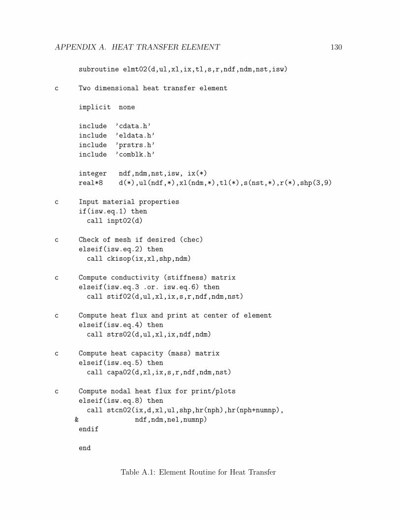
APPENDIX A. HEAT TRANSFER ELEMENT 130
subroutine elmt02(d,ul,xl,ix,tl,s,r,ndf,ndm,nst,isw)
c Two dimensional heat transfer element
implicit none
include ’cdata.h’
include ’eldata.h’
include ’prstrs.h’
include ’comblk.h’
integer ndf,ndm,nst,isw, ix(*)
real*8 d(*),ul(ndf,*),xl(ndm,*),tl(*),s(nst,*),r(*),shp(3,9)
c Input material properties
if(isw.eq.1) then
call inpt02(d)
c Check of mesh if desired (chec)
elseif(isw.eq.2) then
call ckisop(ix,xl,shp,ndm)
c Compute conductivity (stiffness) matrix
elseif(isw.eq.3 .or. isw.eq.6) then
call stif02(d,ul,xl,ix,s,r,ndf,ndm,nst)
c Compute heat flux and print at center of element
elseif(isw.eq.4) then
call strs02(d,ul,xl,ix,ndf,ndm)
c Compute heat capacity (mass) matrix
elseif(isw.eq.5) then
call capa02(d,xl,ix,s,r,ndf,ndm,nst)
c Compute nodal heat flux for print/plots
elseif(isw.eq.8) then
call stcn02(ix,d,xl,ul,shp,hr(nph),hr(nph+numnp),
& ndf,ndm,nel,numnp)
endif
end
Table A.1: Element Routine for Heat Transfer
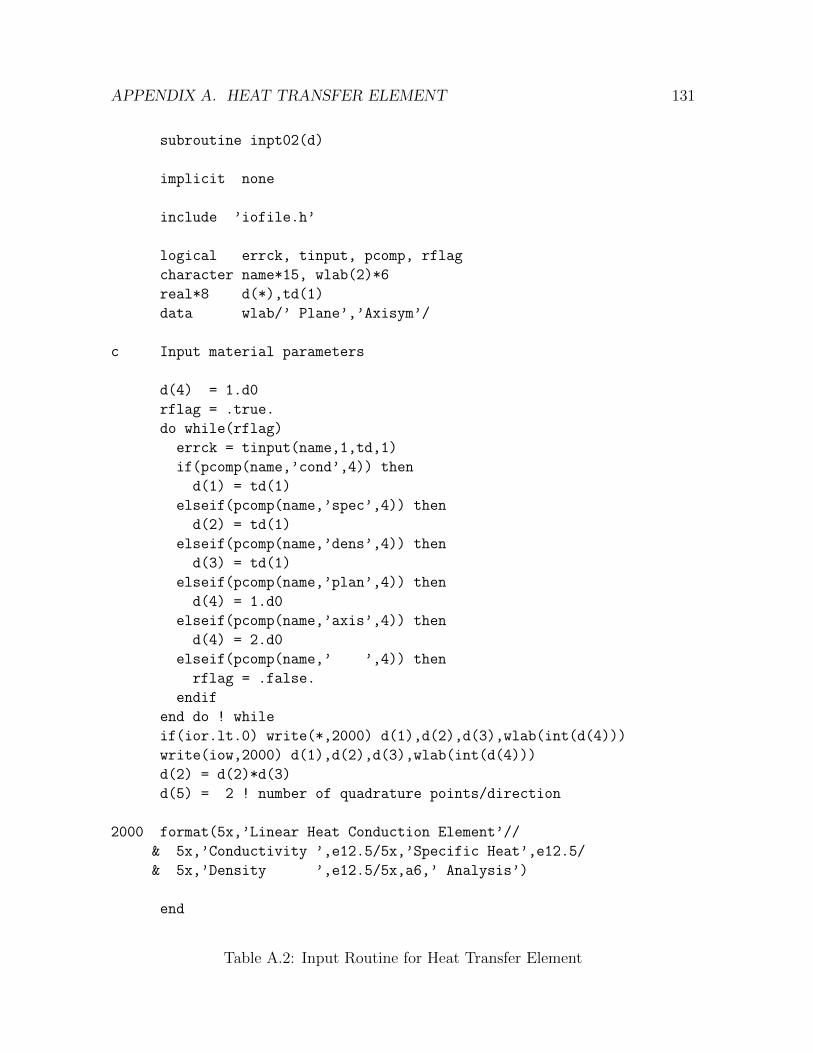
APPENDIX A. HEAT TRANSFER ELEMENT 131
subroutine inpt02(d)
implicit none
include ’iofile.h’
logical errck, tinput, pcomp, rflag
character name*15, wlab(2)*6
real*8 d(*),td(1)
data wlab/’ Plane’,’Axisym’/
c Input material parameters
d(4) = 1.d0
rflag = .true.
do while(rflag)
errck = tinput(name,1,td,1)
if(pcomp(name,’cond’,4)) then
d(1) = td(1)
elseif(pcomp(name,’spec’,4)) then
d(2) = td(1)
elseif(pcomp(name,’dens’,4)) then
d(3) = td(1)
elseif(pcomp(name,’plan’,4)) then
d(4) = 1.d0
elseif(pcomp(name,’axis’,4)) then
d(4) = 2.d0
elseif(pcomp(name,’ ’,4)) then
rflag = .false.
endif
end do ! while
if(ior.lt.0) write(*,2000) d(1),d(2),d(3),wlab(int(d(4)))
write(iow,2000) d(1),d(2),d(3),wlab(int(d(4)))
d(2) = d(2)*d(3)
d(5) = 2 ! number of quadrature points/direction
2000 format(5x,’Linear Heat Conduction Element’//
& 5x,’Conductivity ’,e12.5/5x,’Specific Heat’,e12.5/
& 5x,’Density ’,e12.5/5x,a6,’ Analysis’)
end
Table A.2: Input Routine for Heat Transfer Element
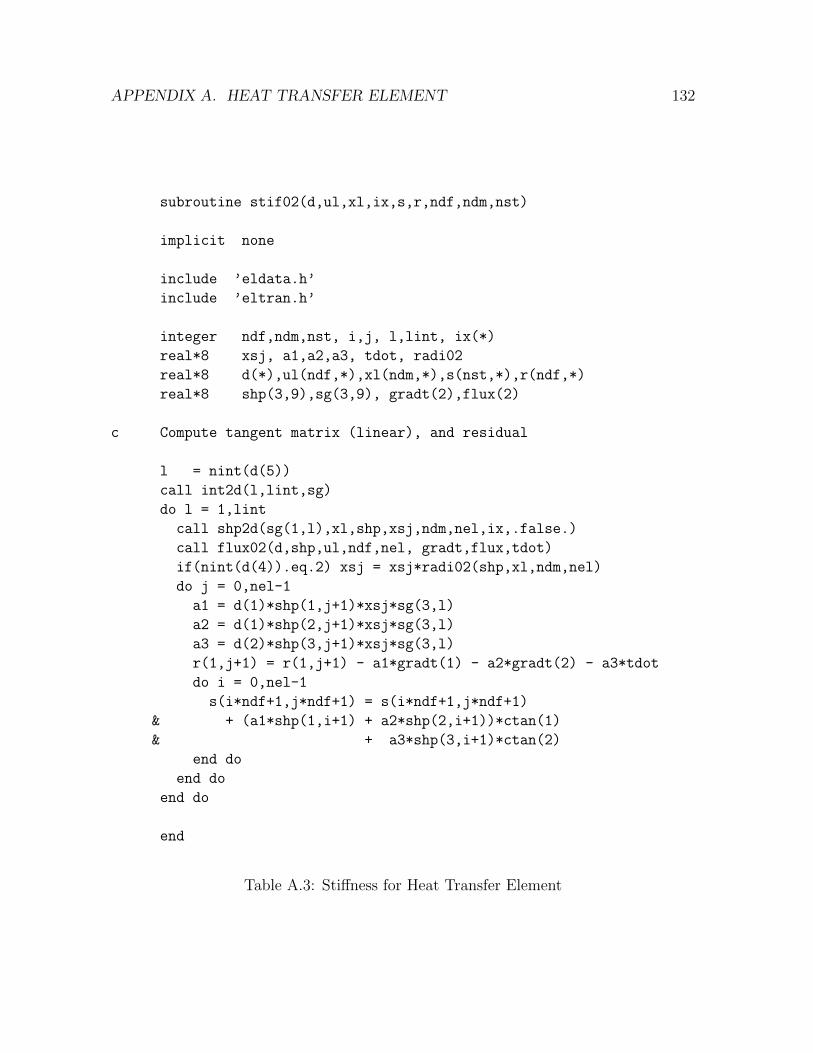
APPENDIX A. HEAT TRANSFER ELEMENT 132
subroutine stif02(d,ul,xl,ix,s,r,ndf,ndm,nst)
implicit none
include ’eldata.h’
include ’eltran.h’
integer ndf,ndm,nst, i,j, l,lint, ix(*)
real*8 xsj, a1,a2,a3, tdot, radi02
real*8 d(*),ul(ndf,*),xl(ndm,*),s(nst,*),r(ndf,*)
real*8 shp(3,9),sg(3,9), gradt(2),flux(2)
c Compute tangent matrix (linear), and residual
l = nint(d(5))
call int2d(l,lint,sg)
do l = 1,lint
call shp2d(sg(1,l),xl,shp,xsj,ndm,nel,ix,.false.)
call flux02(d,shp,ul,ndf,nel, gradt,flux,tdot)
if(nint(d(4)).eq.2) xsj = xsj*radi02(shp,xl,ndm,nel)
do j = 0,nel-1
a1 = d(1)*shp(1,j+1)*xsj*sg(3,l)
a2 = d(1)*shp(2,j+1)*xsj*sg(3,l)
a3 = d(2)*shp(3,j+1)*xsj*sg(3,l)
r(1,j+1) = r(1,j+1) - a1*gradt(1) - a2*gradt(2) - a3*tdot
do i = 0,nel-1
s(i*ndf+1,j*ndf+1) = s(i*ndf+1,j*ndf+1)
& + (a1*shp(1,i+1) + a2*shp(2,i+1))*ctan(1)
& + a3*shp(3,i+1)*ctan(2)
end do
end do
end do
end
Table A.3: Stiffness for Heat Transfer Element
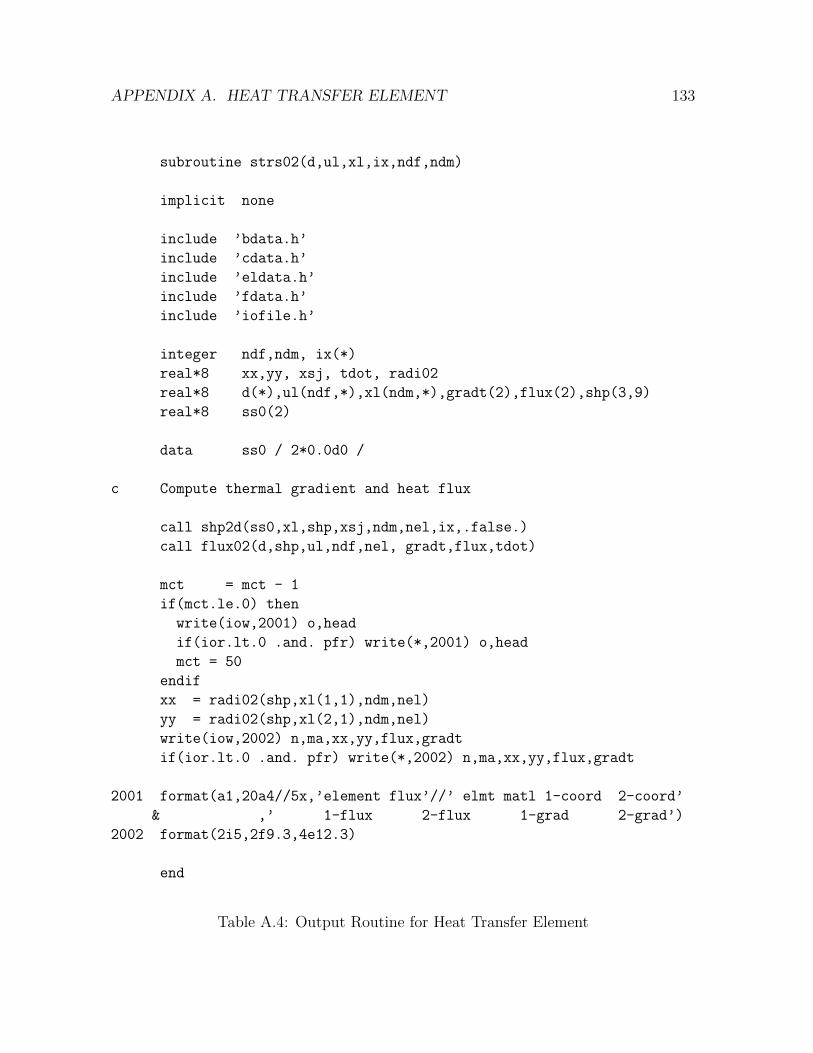
APPENDIX A. HEAT TRANSFER ELEMENT 133
subroutine strs02(d,ul,xl,ix,ndf,ndm)
implicit none
include ’bdata.h’
include ’cdata.h’
include ’eldata.h’
include ’fdata.h’
include ’iofile.h’
integer ndf,ndm, ix(*)
real*8 xx,yy, xsj, tdot, radi02
real*8 d(*),ul(ndf,*),xl(ndm,*),gradt(2),flux(2),shp(3,9)
real*8 ss0(2)
data ss0 / 2*0.0d0 /
c Compute thermal gradient and heat flux
call shp2d(ss0,xl,shp,xsj,ndm,nel,ix,.false.)
call flux02(d,shp,ul,ndf,nel, gradt,flux,tdot)
mct = mct - 1
if(mct.le.0) then
write(iow,2001) o,head
if(ior.lt.0 .and. pfr) write(*,2001) o,head
mct = 50
endif
xx = radi02(shp,xl(1,1),ndm,nel)
yy = radi02(shp,xl(2,1),ndm,nel)
write(iow,2002) n,ma,xx,yy,flux,gradt
if(ior.lt.0 .and. pfr) write(*,2002) n,ma,xx,yy,flux,gradt
2001 format(a1,20a4//5x,’element flux’//’ elmt matl 1-coord 2-coord’
& ,’ 1-flux 2-flux 1-grad 2-grad’)
2002 format(2i5,2f9.3,4e12.3)
end
Table A.4: Output Routine for Heat Transfer Element
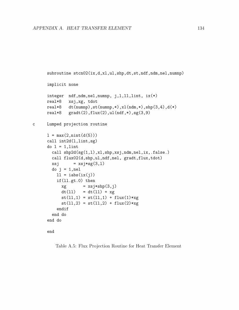
APPENDIX A. HEAT TRANSFER ELEMENT 134
subroutine stcn02(ix,d,xl,ul,shp,dt,st,ndf,ndm,nel,numnp)
implicit none
integer ndf,ndm,nel,numnp, j,l,ll,lint, ix(*)
real*8 xsj,xg, tdot
real*8 dt(numnp),st(numnp,*),xl(ndm,*),shp(3,4),d(*)
real*8 gradt(2),flux(2),ul(ndf,*),sg(3,9)
c Lumped projection routine
l = max(2,nint(d(5)))
call int2d(l,lint,sg)
do l = 1,lint
call shp2d(sg(1,l),xl,shp,xsj,ndm,nel,ix,.false.)
call flux02(d,shp,ul,ndf,nel, gradt,flux,tdot)
xsj = xsj*sg(3,l)
do j = 1,nel
ll = iabs(ix(j))
if(ll.gt.0) then
xg = xsj*shp(3,j)
dt(ll) = dt(ll) + xg
st(ll,1) = st(ll,1) + flux(1)*xg
st(ll,2) = st(ll,2) + flux(2)*xg
endif
end do
end do
end
Table A.5: Flux Projection Routine for Heat Transfer Element
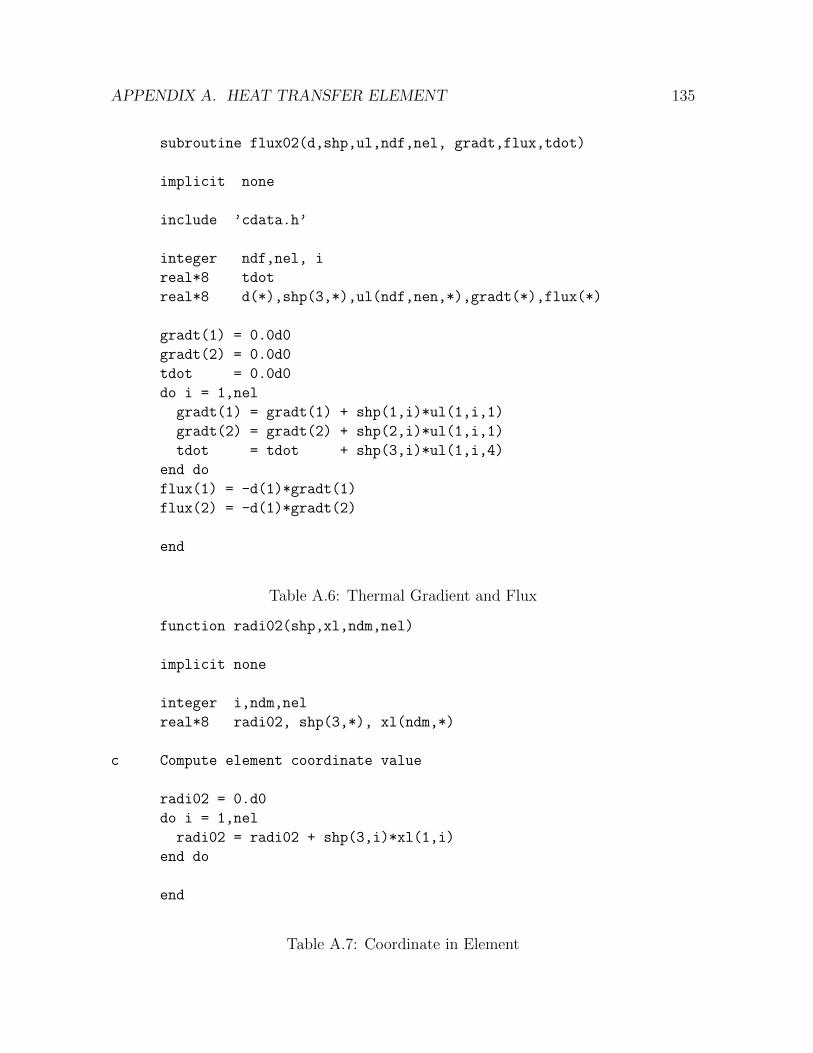
APPENDIX A. HEAT TRANSFER ELEMENT 135
subroutine flux02(d,shp,ul,ndf,nel, gradt,flux,tdot)
implicit none
include ’cdata.h’
integer ndf,nel, i
real*8 tdot
real*8 d(*),shp(3,*),ul(ndf,nen,*),gradt(*),flux(*)
gradt(1) = 0.0d0
gradt(2) = 0.0d0
tdot = 0.0d0
do i = 1,nel
gradt(1) = gradt(1) + shp(1,i)*ul(1,i,1)
gradt(2) = gradt(2) + shp(2,i)*ul(1,i,1)
tdot = tdot + shp(3,i)*ul(1,i,4)
end do
flux(1) = -d(1)*gradt(1)
flux(2) = -d(1)*gradt(2)
end
Table A.6: Thermal Gradient and Flux
function radi02(shp,xl,ndm,nel)
implicit none
integer i,ndm,nel
real*8 radi02, shp(3,*), xl(ndm,*)
c Compute element coordinate value
radi02 = 0.d0
do i = 1,nel
radi02 = radi02 + shp(3,i)*xl(1,i)
end do
end
Table A.7: Coordinate in Element
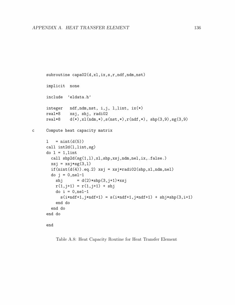
APPENDIX A. HEAT TRANSFER ELEMENT 136
subroutine capa02(d,xl,ix,s,r,ndf,ndm,nst)
implicit none
include ’eldata.h’
integer ndf,ndm,nst, i,j, l,lint, ix(*)
real*8 xsj, shj, radi02
real*8 d(*),xl(ndm,*),s(nst,*),r(ndf,*), shp(3,9),sg(3,9)
c Compute heat capacity matrix
l = nint(d(5))
call int2d(l,lint,sg)
do l = 1,lint
call shp2d(sg(1,l),xl,shp,xsj,ndm,nel,ix,.false.)
xsj = xsj*sg(3,l)
if(nint(d(4)).eq.2) xsj = xsj*radi02(shp,xl,ndm,nel)
do j = 0,nel-1
shj = d(2)*shp(3,j+1)*xsj
r(1,j+1) = r(1,j+1) + shj
do i = 0,nel-1
s(i*ndf+1,j*ndf+1) = s(i*ndf+1,j*ndf+1) + shj*shp(3,i+1)
end do
end do
end do
end
Table A.8: Heat Capacity Routine for Heat Transfer Element
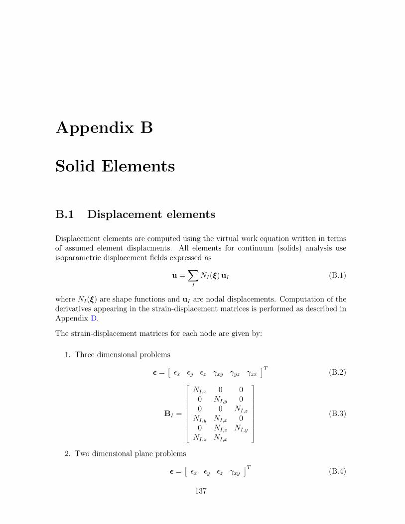
Appendix B
Solid Elements
B.1 Displacement elements
Displacement elements are computed using the virtual work equation written in termsof assumed element displacments. All elements for continuum (solids) analysis useisoparametric displacement fields expressed as
u =∑I
NI(ξ) uI (B.1)
where NI(ξ) are shape functions and uI are nodal displacements. Computation of thederivatives appearing in the strain-displacement matrices is performed as described inAppendix D.
The strain-displacement matrices for each node are given by:
1. Three dimensional problems
ε =[εx εy εz γxy γyz γzx
]T(B.2)
BI =
NI,x 0 0
0 NI,y 00 0 NI,z
NI,y NI,x 00 NI,z NI,y
NI,z NI,x
(B.3)
2. Two dimensional plane problems
ε =[εx εy εz γxy
]T(B.4)
137
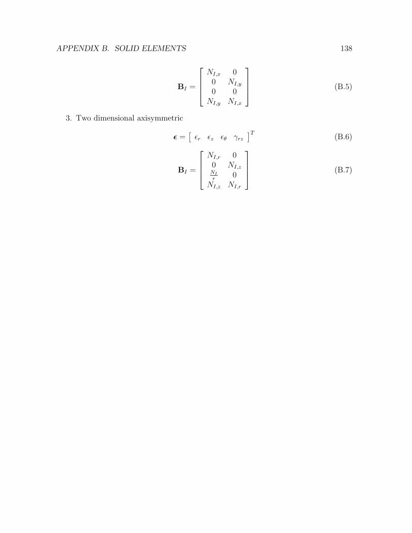
APPENDIX B. SOLID ELEMENTS 138
BI =
NI,x 0
0 NI,y
0 0NI,y NI,x
(B.5)
3. Two dimensional axisymmetric
ε =[εr εz εθ γrz
]T(B.6)
BI =
NI,r 0
0 NI,zNI
r0
NI,z NI,r
(B.7)
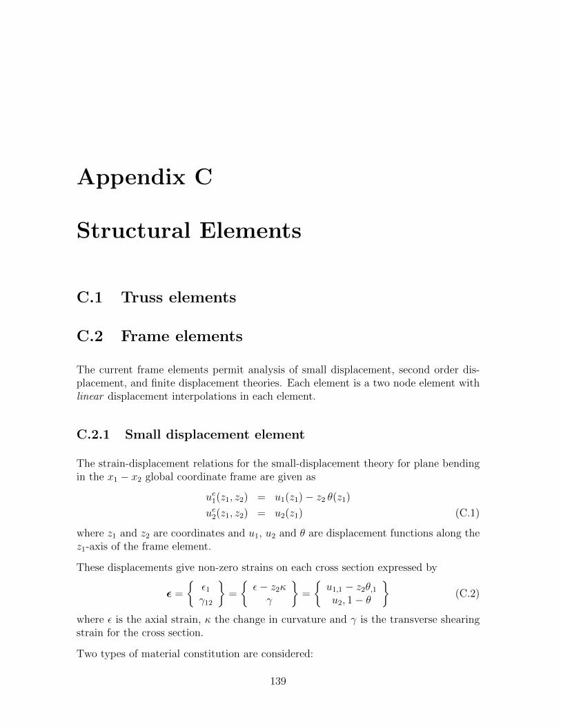
Appendix C
Structural Elements
C.1 Truss elements
C.2 Frame elements
The current frame elements permit analysis of small displacement, second order dis-placement, and finite displacement theories. Each element is a two node element withlinear displacement interpolations in each element.
C.2.1 Small displacement element
The strain-displacement relations for the small-displacement theory for plane bendingin the x1 − x2 global coordinate frame are given as
ue1(z1, z2) = u1(z1)− z2 θ(z1)
ue2(z1, z2) = u2(z1) (C.1)
where z1 and z2 are coordinates and u1, u2 and θ are displacement functions along thez1-axis of the frame element.
These displacements give non-zero strains on each cross section expressed by
ε =
ε1γ12
=
ε− z2κγ
=
u1,1 − z2θ,1u2, 1− θ
(C.2)
where ε is the axial strain, κ the change in curvature and γ is the transverse shearingstrain for the cross section.
Two types of material constitution are considered:
139
APPENDIX C. STRUCTURAL ELEMENTS 140
1. Resultant theory whereNMV
=
EA 0 00 EI 00 0 kGA
εκγ
(C.3)
2. Integration on the cross section whereNM
=
∫A
1z2
σ1(ε− z2κ) dA (C.4)
C.3 Plate elements
C.4 Shell elements
Appendix D
Isoparametric Shape Functions forElements
D.1 Conventional Representation
The shape functions for the bilinear quadrilateral isoparametric element are given by
NI(ξ) =1
4(1 + ξI1 ξ1) (1 + ξI2 ξ2) (D.1)
Using these shape functions, the derivatives with respect to the natural coordinatesare computed to be
∂NI
∂ξ1
=1
4ξI1 (1 + ξI2 ξ2) (D.2)
and∂NI
∂ξ2
=1
4ξI2 (1 + ξI1 ξ1) (D.3)
Using the shape functions, the interpolation for the global Cartesian coordinates maybe expressed in each element as
x = NI(ξ) xI (D.4)
where xI are the values of coordinates at the nodes of the element and the repeatedindex I implies summation over the 4 nodes describing the quadrilateral element.
The derivatives of the shape functions with respect to the global coordinates, x, arecomputed using the chain rule. Accordingly,
∂NI
∂ξα=
∂xi∂ξα
∂NI
∂xi(D.5)
141
APPENDIX D. ISOPARAMETRIC SHAPE FUNCTIONS FOR ELEMENTS 142
which may be written in direct (matrix) notation as
∇ξNI = ∇xNI J (D.6)
When solved for the derivatives with respect to the global coordinates we obtain
∇xNI = ∇ξNI J−1 (D.7)
In the above
∇xNI =
[∂NI
∂x1∂NI
∂x2
](D.8)
∇ξNI =
[∂NI
∂ξ1∂NI
∂ξ2
](D.9)
and
J(ξ) =
[∂x1∂ξ1
∂x1∂ξ2
∂x2∂ξ1
∂x2∂ξ2
](D.10)
Using the shape functions D.1 for the 4-node element, the terms in J(ξ) have thestructure
Jiα =∂xi∂ξα
=1
4
4∑I=1
xIi ξIα +
1
4
4∑I=1
xIi ξIα ξ
Iβ ξβ (D.11)
where1
β = mod(α, 2) + 1 (D.12)
The constant part of J is evaluated at the point ξ = 0 (commonly named the elementcenter), and is given by
∂NI
∂ξα=
1
4ξIα (D.13)
thus
Jiα(0) =∂xi∂ξα
∣∣∣∣ξ=0
=1
4
4∑I=1
xIi ξIα (D.14)
describe the derivatives of the coordinates at the element center. We denote the jaco-bian at the center as J0, that is
J0 = J(0) (D.15)
The global derivatives of the shape functions at the element center become
∇xNI(0) = ∇xiNI(0) J−10 (D.16)
1Note that mod(i, j) = i − ij j where i
j is evaluated in integer arithmetic. Thus, mod(1, 2) and
mod(3, 2) are both evaluated to be 1, while mod(2, 2) and mod(4, 2) are 0.
APPENDIX D. ISOPARAMETRIC SHAPE FUNCTIONS FOR ELEMENTS 143
In subsequent developments we use the notation
biI =∂NI
∂xi
∣∣∣∣ξ=0
(D.17)
to denote the derivatives of the shape functions at the element center.
In subsequent descriptions we will define
∆ Jiαβ =1
4
4∑I=1
xIi ξIα ξ
Iβ =
1
4
4∑I=1
xIi ξI1 ξ
I2 = ∆ Ji (D.18)
which is the coefficient to the spatially varying part of the jacobian transformation.That is, the jacobian determinant may be expressed as[
J11(ξ) J12(ξ)J21(ξ) J22(ξ)
]=
[(J0)11 (J0)21
(J0)21 (J0)22
]+
[∆J112 ξ2 ∆J121 ξ1
∆J212 ξ2 ∆J221 ξ1
](D.19)
which in matrix notation may be written as
J(ξ) = J0 + ∆J Ξ (D.20)
where
Ξ =
[ξ2 00 ξ1
](D.21)
and
∆J =
[∆J1 ∆J1
∆J2 ∆J2
](D.22)
D.2 Alternative Representation in Two Dimensions
An alternative representation for the shape functions has been proposed by Belytschko.In the development of stabilized elements he introduced the representation
NI(ξ) =1
4δI +
2∑i=1
biI (xi − x0i ) + ΓI h(ξ) (D.23)
where xi are the element global cartesian coordinates,
x0i =
4∑I=1
xIi NI(0) =1
4(x1
i + x2i + x3
i + x4i ) (D.24)
are the values of the global coordinates at the element center,
h(ξ) = ξ1 ξ2 (D.25)
APPENDIX D. ISOPARAMETRIC SHAPE FUNCTIONS FOR ELEMENTS 144
and δI and ΓI are constant parameters associated with node I. These parameters maybe evaluated by defining the shape functions at each node and using the fact that
NI(ξJ) = δIJ (D.26)
where δIJ is the Kronecker delta function for the nodes. Evaluating the alternativeshape function expression at each node gives
NI(ξJ) =1
4δI +
2∑i=1
biI (xJi − x0i ) + ΓI h(ξJ) (D.27)
Introducing the notation1T =
[1 1 1 1
](D.28)
hT =[1 −1 1 −1
](D.29)
xTi =[x1i x2
i x3i x4
i
](D.30)
bTi =[bi1 bi2 bi3 bi4
](D.31)
and the parameter vectorsδT =
[δ1 δ2 δ3 δ4
](D.32)
ΓT =[Γ1 Γ2 Γ3 Γ4
](D.33)
The shape functions at the nodes may be written in the matrix form
I =1
4δ 1T +
2∑i=1
bi (xi − x0i 1)T + Γ hT (D.34)
Note that the rows in the expression are associated with the I in the NI shape functions,while the columns are associated with the J where the ξJ are evaluated. The I is a4 × 4 identity matrix for the element. Using this form, the parameters δ and Γ maybe easily computed. First by multiplying (from the right) by 1, we obtain
I 1 = 1 = δ (D.35)
In obtaining this result we note that
1T 1 = 4 (D.36)
andxTi 1 = 4x0
i (D.37)
which gives(xi − x0
i 1)T 1 = 0 (D.38)
Finally, we note thathT 1 = 0 (D.39)
APPENDIX D. ISOPARAMETRIC SHAPE FUNCTIONS FOR ELEMENTS 145
Next by multiplying (again from the right) by h, we get
hT h = 4 (D.40)
I h = h =2∑i=1
xhi bi + 4 Γ (D.41)
where2
xhi = xTi h (D.42)
Thus, the parameters for Γ are computed as
Γ =1
4[h −
2∑i=1
xhi bi] (D.43)
It remains to compute the bi.
D.3 Derivatives of Alternative Formulation
Using the alternative expression for the shape functions, the derivatives with respectto the global coordinates, xi, are given by
∂NI
∂xi= biI + ΓI
∂h
∂xi(D.44)
where the biI are constant over the entire element and are computed by the conventionalexpressions at the center of the element. The derivatives of the function h may also becomputed using the chain rule and are given by
∇x h = ∇ξ hJ−1 (D.45)
For the specific functional expression for h, the gradient with respect to the naturalcoordinates is given by
∇ξ h =
[ξ2
ξ1
](D.46)
Furthermore, the inverse for the jacobian matrix is given by
J−1 =1
j(ξ)
[∂x2∂ξ2
−∂x1∂ξ2
−∂x2∂ξ1
∂x1∂ξ1
](D.47)
2The factor xhi is sometimes called an hour glass shape, and when the coordinate, x, is replacedby the displacement, u, the factor uhi , defines the magnitude of the hour glass mode.
APPENDIX D. ISOPARAMETRIC SHAPE FUNCTIONS FOR ELEMENTS 146
where j(ξ) is the determinant of the jacobian transformation matrix, J. Recall that thederivative of a global coordinate with respect to a natural coordinate has a constantand a linear part. For the specific form of the h(ξ) function the product of the linearpart vanishes and the relationship for the gradient simplifies to
∇x h =j0
j(ξ)∇ξ hJ−1
0 (D.48)
where j0 is the value of the jacobian determinant evaluated at the element center. Thejacobian determinant at the center of the element is computed to be
j0 = (J0)11 (J0)22 − (J0)21 (J0)12 (D.49)
We note also that the jacobian determinant at any location in the element may beexpressed as
j(ξ) = j0 + j1 ξ1 + j2 ξ2 (D.50)
wherej1 = (J0)11 ∆ J22 − (J0)21 ∆ J12 (D.51)
j2 = ∆ J11 (J0)22 − ∆ J21 (J0)12 (D.52)
With the above definitions and
bI =
[b1I
b2I
](D.53)
the gradient of the displacement may be written as
∇x u = ∇xNI uI =
[bI +
j0
j(ξ)∇ξ hJ−1
0 ΓI
]uI (D.54)
The structure of this representation is useful knowledge when we consider the construc-tion of the enhanced part of the strains in Chapter 8.
Appendix E
Properties for J2 plasticity models
The solution of the J2 plasticity model leads to derivatives of the yield and loadingfunctions in the form
∂f
∂Σ= n (E.1)
where
n =Σ
‖ Σ ‖(E.2)
andΣ = s − α (E.3)
We note that n has the properties
1T n = 0 ; nT n = 1 (E.4)
In the derivation of the tangent the derivative of n leads to
∂2f
∂Σ ∂Σ=
∂n
∂Σ=
1
‖ Σ ‖(1 − n nT ) (E.5)
which appears in several location in the tangent matrices. The inversion of the tangentmatrices may be simplified using the Sherman-Morrison-Woodbury formula[6] whichgives
(A + U VT )−1 = A−1 − A−1 U W VT A−1 (E.6)
whereW = (I + VT A−1 U)−1 (E.7)
In the above A is an ntimesn matrix, U,V are n× k matrices, where k ≤ n, and Wis a k × k matrix. The inverse may be proved by multiplying the results together torecover the identity matrix. In the case of the deviatoric model A is diagonal and U
147
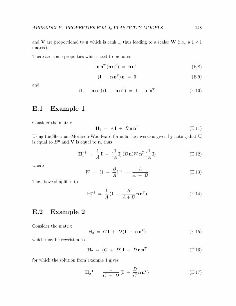
APPENDIX E. PROPERTIES FOR J2 PLASTICITY MODELS 148
and V are proportional to n which is rank 1, thus leading to a scalar W (i.e., a 1× 1matrix).
There are some properties which need to be noted:
n nT (n nT ) = n nT (E.8)
(I − n nT ) n = 0 (E.9)
and(I − n nT ) (I − n nT ) = I − n nT (E.10)
E.1 Example 1
Consider the matrixH1 = A I + B n nT (E.11)
Using the Sherman-Morrison-Woodward formula the inverse is given by noting that Uis equal to Bn and V is equal to n, thus
H−11 =
1
AI − (
1
AI) (B n)W nT (
1
AI) (E.12)
where
W = (1 +B
A)−1 =
A
A + B(E.13)
The above simplifies to
H−11 =
1
A(I − B
A+Bn nT ) (E.14)
E.2 Example 2
Consider the matrixH2 = C I + D (I − n nT ) (E.15)
which may be rewritten as
H2 = (C + D) I − D n nT (E.16)
for which the solution from example 1 gives
H−12 =
1
C + D(I +
D
Cn nT ) (E.17)
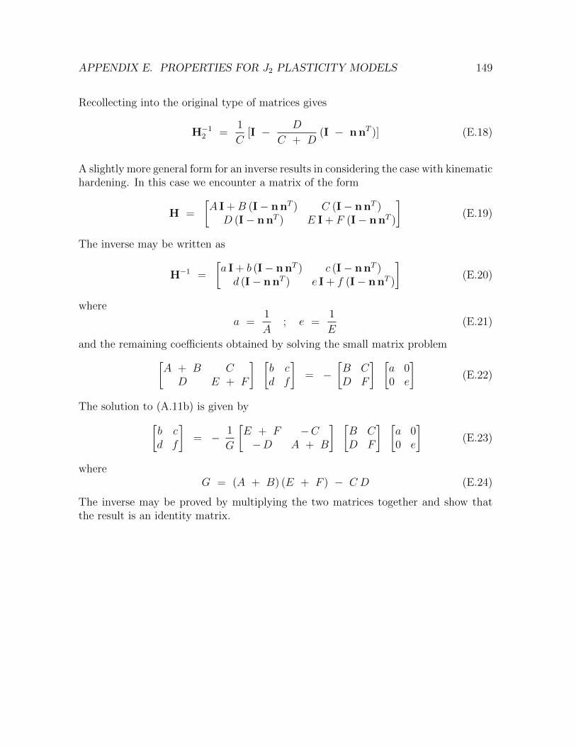
APPENDIX E. PROPERTIES FOR J2 PLASTICITY MODELS 149
Recollecting into the original type of matrices gives
H−12 =
1
C[I − D
C + D(I − n nT )] (E.18)
A slightly more general form for an inverse results in considering the case with kinematichardening. In this case we encounter a matrix of the form
H =
[A I +B (I− n nT ) C (I− n nT )D (I− n nT ) E I + F (I− n nT )
](E.19)
The inverse may be written as
H−1 =
[a I + b (I− n nT ) c (I− n nT )d (I− n nT ) e I + f (I− n nT )
](E.20)
where
a =1
A; e =
1
E(E.21)
and the remaining coefficients obtained by solving the small matrix problem[A + B C
D E + F
] [b cd f
]= −
[B CD F
] [a 00 e
](E.22)
The solution to (A.11b) is given by[b cd f
]= − 1
G
[E + F −C−D A + B
] [B CD F
] [a 00 e
](E.23)
whereG = (A + B) (E + F ) − C D (E.24)
The inverse may be proved by multiplying the two matrices together and show thatthe result is an identity matrix.
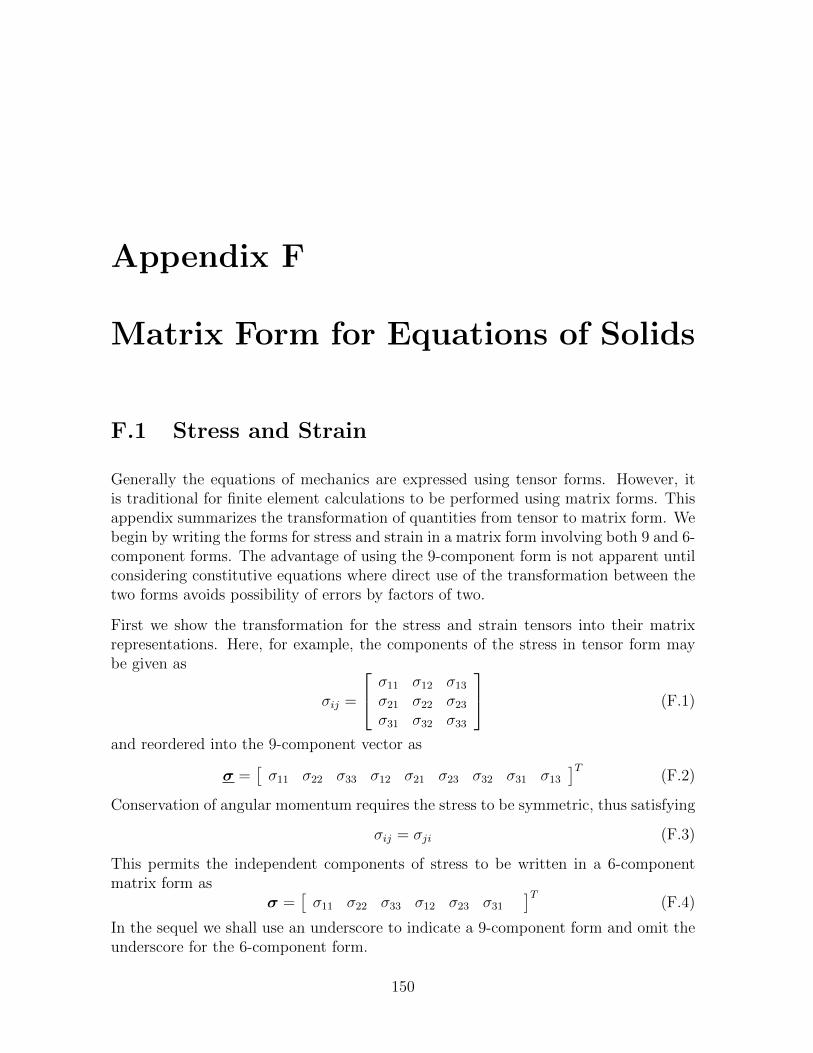
Appendix F
Matrix Form for Equations of Solids
F.1 Stress and Strain
Generally the equations of mechanics are expressed using tensor forms. However, itis traditional for finite element calculations to be performed using matrix forms. Thisappendix summarizes the transformation of quantities from tensor to matrix form. Webegin by writing the forms for stress and strain in a matrix form involving both 9 and 6-component forms. The advantage of using the 9-component form is not apparent untilconsidering constitutive equations where direct use of the transformation between thetwo forms avoids possibility of errors by factors of two.
First we show the transformation for the stress and strain tensors into their matrixrepresentations. Here, for example, the components of the stress in tensor form maybe given as
σij =
σ11 σ12 σ13
σ21 σ22 σ23
σ31 σ32 σ33
(F.1)
and reordered into the 9-component vector as
σ =[σ11 σ22 σ33 σ12 σ21 σ23 σ32 σ31 σ13
]T(F.2)
Conservation of angular momentum requires the stress to be symmetric, thus satisfying
σij = σji (F.3)
This permits the independent components of stress to be written in a 6-componentmatrix form as
σ =[σ11 σ22 σ33 σ12 σ23 σ31
]T(F.4)
In the sequel we shall use an underscore to indicate a 9-component form and omit theunderscore for the 6-component form.
150
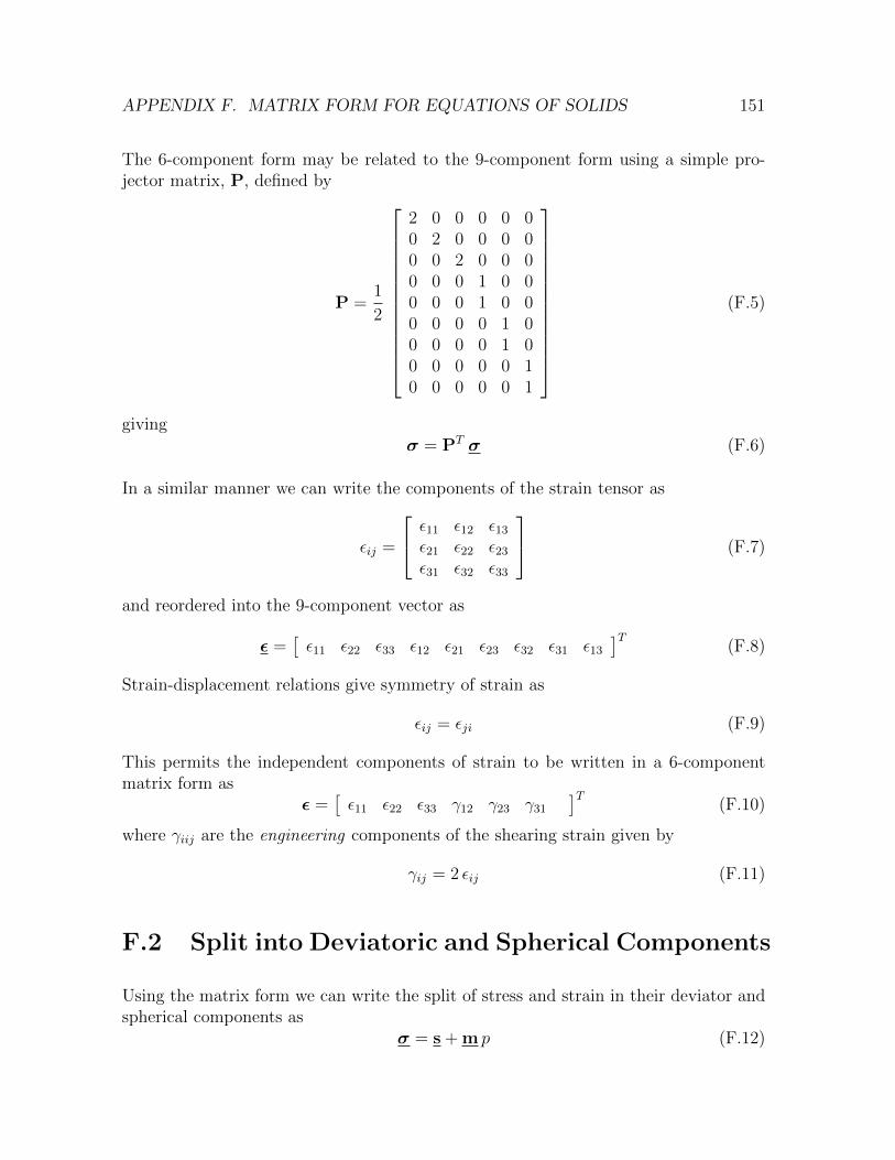
APPENDIX F. MATRIX FORM FOR EQUATIONS OF SOLIDS 151
The 6-component form may be related to the 9-component form using a simple pro-jector matrix, P, defined by
P =1
2
2 0 0 0 0 00 2 0 0 0 00 0 2 0 0 00 0 0 1 0 00 0 0 1 0 00 0 0 0 1 00 0 0 0 1 00 0 0 0 0 10 0 0 0 0 1
(F.5)
givingσ = PT σ (F.6)
In a similar manner we can write the components of the strain tensor as
εij =
ε11 ε12 ε13
ε21 ε22 ε23
ε31 ε32 ε33
(F.7)
and reordered into the 9-component vector as
ε =[ε11 ε22 ε33 ε12 ε21 ε23 ε32 ε31 ε13
]T(F.8)
Strain-displacement relations give symmetry of strain as
εij = εji (F.9)
This permits the independent components of strain to be written in a 6-componentmatrix form as
ε =[ε11 ε22 ε33 γ12 γ23 γ31
]T(F.10)
where γiij are the engineering components of the shearing strain given by
γij = 2 εij (F.11)
F.2 Split into Deviatoric and Spherical Components
Using the matrix form we can write the split of stress and strain in their deviator andspherical components as
σ = s + m p (F.12)
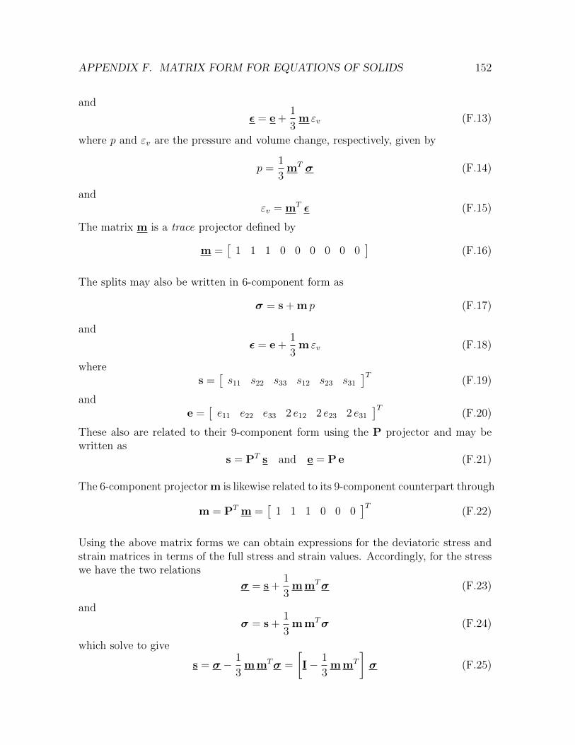
APPENDIX F. MATRIX FORM FOR EQUATIONS OF SOLIDS 152
and
ε = e +1
3m εv (F.13)
where p and εv are the pressure and volume change, respectively, given by
p =1
3mT σ (F.14)
andεv = mT ε (F.15)
The matrix m is a trace projector defined by
m =[
1 1 1 0 0 0 0 0 0]
(F.16)
The splits may also be written in 6-component form as
σ = s + m p (F.17)
and
ε = e +1
3m εv (F.18)
wheres =
[s11 s22 s33 s12 s23 s31
]T(F.19)
ande =
[e11 e22 e33 2 e12 2 e23 2 e31
]T(F.20)
These also are related to their 9-component form using the P projector and may bewritten as
s = PT s and e = P e (F.21)
The 6-component projector m is likewise related to its 9-component counterpart through
m = PT m =[
1 1 1 0 0 0]T
(F.22)
Using the above matrix forms we can obtain expressions for the deviatoric stress andstrain matrices in terms of the full stress and strain values. Accordingly, for the stresswe have the two relations
σ = s +1
3m mTσ (F.23)
and
σ = s +1
3m mTσ (F.24)
which solve to give
s = σ − 1
3m mTσ =
[I− 1
3m mT
]σ (F.25)
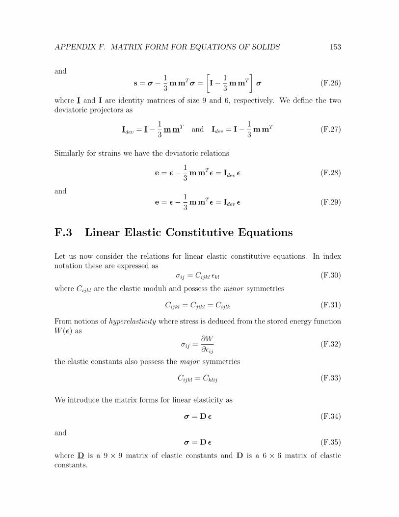
APPENDIX F. MATRIX FORM FOR EQUATIONS OF SOLIDS 153
and
s = σ − 1
3m mTσ =
[I− 1
3m mT
]σ (F.26)
where I and I are identity matrices of size 9 and 6, respectively. We define the twodeviatoric projectors as
Idev = I− 1
3m mT and Idev = I− 1
3m mT (F.27)
Similarly for strains we have the deviatoric relations
e = ε− 1
3m mTε = Idev ε (F.28)
and
e = ε− 1
3m mTε = Idev ε (F.29)
F.3 Linear Elastic Constitutive Equations
Let us now consider the relations for linear elastic constitutive equations. In indexnotation these are expressed as
σij = Cijkl εkl (F.30)
where Cijkl are the elastic moduli and possess the minor symmetries
Cijkl = Cjikl = Cijlk (F.31)
From notions of hyperelasticity where stress is deduced from the stored energy functionW (ε) as
σij =∂W
∂εij(F.32)
the elastic constants also possess the major symmetries
Cijkl = Cklij (F.33)
We introduce the matrix forms for linear elasticity as
σ = D ε (F.34)
andσ = D ε (F.35)
where D is a 9 × 9 matrix of elastic constants and D is a 6 × 6 matrix of elasticconstants.
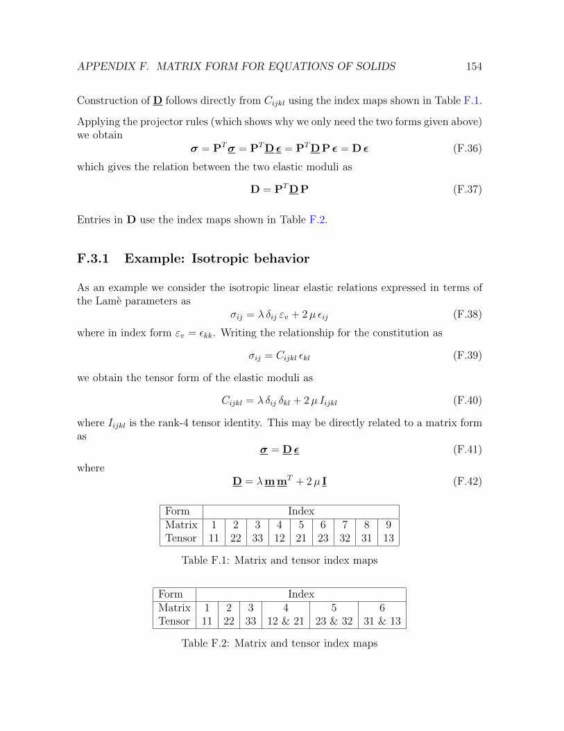
APPENDIX F. MATRIX FORM FOR EQUATIONS OF SOLIDS 154
Construction of D follows directly from Cijkl using the index maps shown in Table F.1.
Applying the projector rules (which shows why we only need the two forms given above)we obtain
σ = PTσ = PTD ε = PTD P ε = D ε (F.36)
which gives the relation between the two elastic moduli as
D = PTD P (F.37)
Entries in D use the index maps shown in Table F.2.
F.3.1 Example: Isotropic behavior
As an example we consider the isotropic linear elastic relations expressed in terms ofthe Lame parameters as
σij = λ δij εv + 2µ εij (F.38)
where in index form εv = εkk. Writing the relationship for the constitution as
σij = Cijkl εkl (F.39)
we obtain the tensor form of the elastic moduli as
Cijkl = λ δij δkl + 2µ Iijkl (F.40)
where Iijkl is the rank-4 tensor identity. This may be directly related to a matrix formas
σ = D ε (F.41)
whereD = λm mT + 2µ I (F.42)
Form IndexMatrix 1 2 3 4 5 6 7 8 9Tensor 11 22 33 12 21 23 32 31 13
Table F.1: Matrix and tensor index maps
Form IndexMatrix 1 2 3 4 5 6Tensor 11 22 33 12 & 21 23 & 32 31 & 13
Table F.2: Matrix and tensor index maps
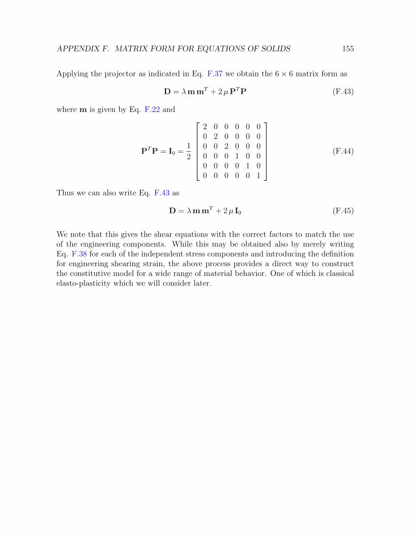
APPENDIX F. MATRIX FORM FOR EQUATIONS OF SOLIDS 155
Applying the projector as indicated in Eq. F.37 we obtain the 6× 6 matrix form as
D = λm mT + 2µPTP (F.43)
where m is given by Eq. F.22 and
PTP = I0 =1
2
2 0 0 0 0 00 2 0 0 0 00 0 2 0 0 00 0 0 1 0 00 0 0 0 1 00 0 0 0 0 1
(F.44)
Thus we can also write Eq. F.43 as
D = λm mT + 2µ I0 (F.45)
We note that this gives the shear equations with the correct factors to match the useof the engineering components. While this may be obtained also by merely writingEq. F.38 for each of the independent stress components and introducing the definitionfor engineering shearing strain, the above process provides a direct way to constructthe constitutive model for a wide range of material behavior. One of which is classicalelasto-plasticity which we will consider later.