Embed Size (px)
DESCRIPTION
Eurostat/UNECE Work Session on Demographic Projections Lee-Carter Mortality Projection with "Limit Life Table" Jorge Miguel Bravo University of Évora (Deparment of Economics) and CEFAGE -UE Lisbon , Portugal, 29 th April 2010. Introduction and motivation - PowerPoint PPT Presentation
Citation preview

© Jorge Miguel Bravo 1
Eurostat/UNECE Work Session on Demographic Projections
Lee-Carter Mortality Projection
with "Limit Life Table"
Jorge Miguel Bravo
University of Évora (Deparment of Economics) and CEFAGE -UE
Lisbon, Portugal, 29th April 2010

© Jorge Miguel Bravo 2
1. Introduction and motivation
2. Classical Lee-Carter mortality modelling
3. Lee-Carter Model with "Limit Life Table“
4. Implementation issues
5. Concluding remarks and further research
Agenda

© Jorge Miguel Bravo 3
• Mortality forecasting methods currently can be classified into
1. Explanatory methods
Based on structural or causal epidemiological models, analyze the
relationship between age-specific risk factors (e.g., smoking) and
mortality rates
2. Expert-opinion based methods
Involve the use of informed expectations about the future,
alternative low/high scenarios or a targeting approach
3. Extrapolative methods
Assume that future mortality patterns can be estimated by
projecting into the future trends observed in the recent to
medium-term past (e.g., Lee-Carter, APC methods)
Mortality forecasting methods

© Jorge Miguel Bravo 4
• Why do we use extrapolative methods? Because...
– of the inherent complexity of the factors affecting
human mortality
– of the current lack of understanding of the intricate
mechanisms governing the aging process
– of the relative stability of the past demographic trends
– they offer a reliable basis for projection
• So what’s the problem?
“... using extrapolative methods is like driving a car through
the rear mirror ...!”
Extrapolative methods

© Jorge Miguel Bravo 5
• Since the methods rely on the assumption that future
mortality trends will continue into the future as observed in
the past, they may
– generate biologically implausible scenarios (e.g., null
mortality rates for all ages)
– produce implausible age patterns
Crossover of consecutive mortality rates
Crossover of male/female life expectancy
– produce increasing divergence in life expectancy
Extrapolative methods: limitations

© Jorge Miguel Bravo 6
• Age-Period demographic model
• Identification constraints
• Fitting method: OLS by Singular Value Decomposition (SVD)
• Forecasting: Age effects (x and x) are assumed constant + a time
series ARIMA (p,d,q) model for the time component (kt)
• Problem: Asymptotic behavior of the model
Classical AP Lee-Carter model
2
, , ,ln , (0, )x t x x t x t x tm k N
max max
min min
1, 0x t
x tx x t t
k
,ˆ ˆˆˆlim lim exp ˆ 0x t x x tk k
m k

© Jorge Miguel Bravo 7
AP Lee-Carter model

© Jorge Miguel Bravo 8
• Basic idea (Bravo, 2007)
– There is a “target” life table to which longevity improvements
over time (over a projection horizon) converge
– We explicitly admit that there are (at least in a limited time
horizon) natural limits to longevity improvements
• Rationale
– there is a decline in the physiological parameters associated
with ageing in humans duration of life is limited?
– stylized facts: slowdown in life expectancy at birth increases
observed in many developed countries
AP LC Model with “Limit Life Table”

© Jorge Miguel Bravo 9
• Hip. 1: the age-specific forces of mortality are constant within
each rectangle of the Lexis diagram
• Hip. 2: Let denote the instantaneous death rate or
probability of death corresponding to this “target” life table
• Hip. 3: AP LC model is formulated within a Generalized Linear
Model (GLM) framework with a generalized error distribution
age- and period-specific numbers of deaths are independent
realizations from a Poisson distribution with parameters
AP LC Model with “Limit Life Table”
lim lim,x xq
, , , for 0 , 1x t x t
, , , , ,, x t x t x t x t x tE D E Var D E D

© Jorge Miguel Bravo 10
• Age-Period demographic model
with
identification constraints
• GLM model of the response variable Dx,t with logarithmic link and
non-linear parameterized predictor
AP LC Model with “Limit Life Table”
lim
, ,
ad
x t x x t
max max
min min
1, 0x t
x tx x t t
k
, expad
x t x x tk
lim
, ,log logx t x t x x x tE k
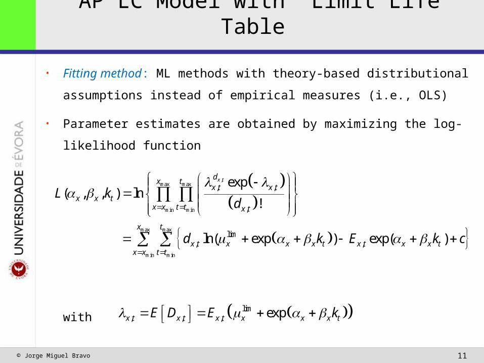
© Jorge Miguel Bravo 11
• Fitting method: ML methods with theory-based distributional
assumptions instead of empirical measures (i.e., OLS)
• Parameter estimates are obtained by maximizing the log-likelihood
function
with
AP LC Model with “Limit Life Table”
,max max
min min
max max
min min
, ,
,
lim, ,
exp( , , ) ln
!
ln( exp ) exp( )
x tdx tx t x t
x x tx x t t x t
x t
x t x x x t x t x x tx x t t
L kd
d k E k c
lim, , , expx t x t x t x x x tE D E k

© Jorge Miguel Bravo 12
• Because of the log-bilinear term xkt we cannot use standard
statistical packages that include GLM Poisson regression
• Solution: Use an iterative algorithm for estimating log-bilinear
models developed by Goodman (1979) based on a Newton-
Raphson algorithm Updating-scheme
• Adjust parameter estimates to meet identification constraints
• Forecasting: Age effects (x and x) constant and a time series
ARIMA (p,d,q) model for the time component (kt)
AP LC Model with “Limit Life Table”
( )
( 1) ( )2 ( )
2
( , , )
ˆˆ ˆ ˆ ˆˆ, , ,( , , )
vx x t
jv vj j x x tv
x x t
j
L k
kL k

© Jorge Miguel Bravo 13
• We need a “limit/target” life table as input subjective/informed
assumptions about the future development of a set of important
biological, economic and social variables have to be made
• Alternative approaches
– Use an epidemiological model to define the target life table (TLT)
– Consider the life table of a more advanced population as TLT
– Use the observed gaps between countries and regions
– combination of the lowest mortality rates observed by sex-age groups
– estimates of the lowest achievable cause-specific death rates
– Calibrate some mortality law to express different scenarios on the main
trends in human longevity (e.g., rectangularization survival curve, life
expectancy trends, median, mode, entropy, IQR,...)
Implementation issues
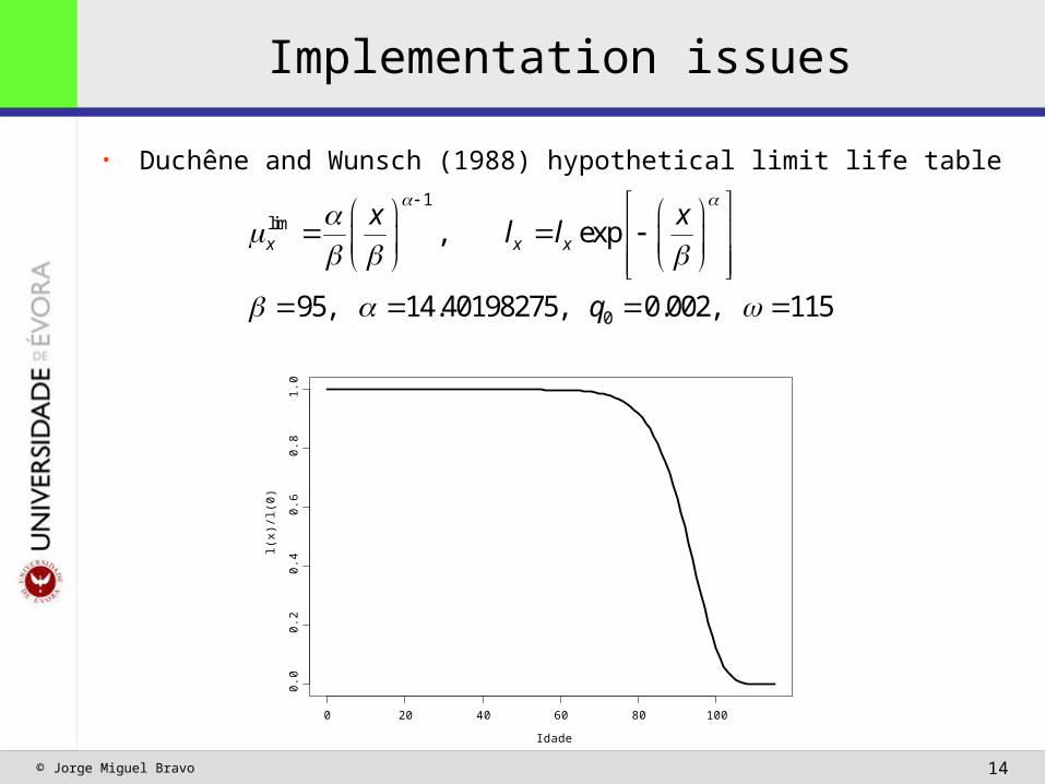
© Jorge Miguel Bravo 14
• Duchêne and Wunsch (1988) hypothetical limit life table
Implementation issues
1lim
0
, exp
95, 14.40198275, 0.002, 115
x x x
x xl l
q
Idade
l(x)/l(0)
0 20 40 60 80 100
0.0
0.2
0.4
0.6
0.8
1.0

© Jorge Miguel Bravo 15
• 2nd Heligman-Pollard (1980) mortality law
Implementation issues
( ) 2exp (ln ln )1
Cx
x Bx x
GHq A D E x F
KGH
Age
ln(mux)
0 20 40 60 80
-10
-8-6
-4-2
Heligman-Pollard2007
© Jorge Miguel Bravo 16
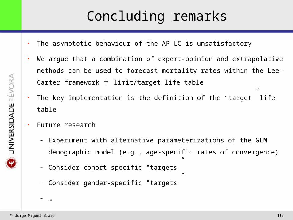
• The asymptotic behaviour of the AP LC is unsatisfactory
• We argue that a combination of expert-opinion and extrapolative
methods can be used to forecast mortality rates within the Lee-
Carter framework limit/target life table
• The key implementation is the definition of the “target” life table
• Future research
– Experiment with alternative parameterizations of the GLM
demographic model (e.g., age-specific rates of convergence)
– Consider cohort-specific “targets”
– Consider gender-specific “targets”
– …
Concluding remarks
© Jorge Miguel Bravo 17
THANK YOUJORGE MIGUEL BRAVO
Eurostat/UNECE Work Session on Demographic Projections