ENGINEERING DESIGN HANDBOOK · 2014-10-02 · amcp 706-196 department of the army headquarters us army materiel command 5001 eisenhower avenue, alexandria, va 22333 amc pamphlet 5

AMC PAMPHLET AMCP 706-196

ENGINEERING DESIGN

HANDBOOK

DEVELOPMENT GUIDE

FOR RELIABILITY

PART TWO

DESIGN. FOR

RELIABILITY

HEADQUARTERS, US ARMY MATERIEL COMMAND JANUARY 1976

AMCP 706-196

DEPARTMENT OF THE ARMY HEADQUARTERS US ARMY MATERIEL COMMAND

5001 EISENHOWER AVENUE, ALEXANDRIA, VA 22333

AMC PAMPHLET 5 January 1976 NO. 706-196

ENGINEERING DESIGN HANDBOOK ~

DESIGN FOR RELIABILITY

TABLE OF CONTENTS

Paragraph Page

IZST OF ILLUSTRATIONS vi LISTOFTABLES viii PREFACE ix

CHAPTER 1. INTRODUCTION

1-0 List of Symbols 1-1 1-1 General 1-1 1-2 System Engineering 1-2 1-3 System Effectiveness 1-4 1-4 The Role cf Reliability 1-7 1-5 The Role of Maintainability 1-9 1-5.1 Relationship to Reliability 1-10 1-5.2 Design Guidelines 1-10 1-5.3 Prediction 1-12 1-5.4 Design Review 1-12 1-5.5 Availability 1-13 1-6 The Role of Safety 1-13 1-6.1 Relationships to Reliability 1-14 1-6.2 System Hazard Analysis 1-14 1-6.3 Trade-offs 1-15 1-7 Summary 1-16

CHAPTER 2. THE ENVIRONMENT

2-1 Introduction 2-1 2-1.1 Military Operations 2-1 2-1.2 Predicting Environmental Conditions 2-1 2-2 Effects of the Environment 2-3 2-2-1 General Categories 2-3 2-2.2 Combinations of Natural Environmental Factors 2-3 2-2.2.1 Evaluation of Environmental Characteristics 2-3 2-2.2.2 Combinations 2-3 2-2.2.3 Practical Combinations . . . 2-7

AMCP 706-196

TABLE OF CONTENTS

Paragraph Page

2-2.3 Combinationsof Induced Environmental Factors 2-8 2-2.4 Environmental Analysis 2-8 2-3 Designing for the Environment 2-8 2-3.1 Temperature Protection 2-14 2-3.2 Shock and Vibration Protection *„ . 2-15 2-3.3 Moisture Protection 2-17 2-3.4 Sand and Dust Protection 2-17 2-3.5 Explosion Proofing 2-18 2-3.6 Electromagnetic-Radiation Protection 2-19 2 4 Operations Research Methods 2-19

CHAPTER 3. MEASURES OF RELIABILITY

3-0 List of Symbols 3-1 3-1 Introduction 3-1 3-2 Probabilities cf Success and Failure 3-1 3-3 Failure Distributions 3-2 3-4 Failure Rate 3-3 3-5 Time-to-Failure 3-5 3-6 Time Between Failures 3-5 3-7 Fraction Defective 3-6

CHAPTER 4. MODEL BUILDING AND ANALYSIS

4-0 List cf Symbols 4-1 41 Introduction 4-1 4-2 Model Building 4-2 4-3 Analysis 4-9 4-4 Simulation 4-9 4-4.1 General Description cf a Simulation Program 4-9 4-5 Computer Programs 4-16

CHAPTER 5. ALLOCATION OF RELIABILITY REQUIREMENTS

5-0 List of Symbols 5-1 5-1 Introduction 5-1 5-2 Systems Without Repair 5-2 5-2.1 Equal Allocation 5-3 5-2.2 Proportional Complexity 5-3 5-2.3 Simple-Modular Complexity 5-3 5-2.4 Detailed Complexity 5-8 5-2.5 Feasibility-of-Objectives Allocations 5-9 5-2.6 Redundant Systems 5-13 5-2.7 Redundant Systars with Constraints 5-13 5-2.7.1 Simple Redundancy Allocation with a

Single Constraint 5-20 5-2.7.2 Dynamic Programming Allocation 5-20 5-2.7.3 Minimization of Effort Algorithm 5-20 5-3 Systems with Repair .- 5-23

■1

AMCP 706-196

TABLE OF CONTENTS

Paragraph Page

5-3.1 An Elementary Approach to Steady-State Availability .» .... 5-23

5-3.2 Failure Rate and Repair Rate Allocation €orSeries Systems 5-25

5-3.3 A Simple Technique for Allocating Steady-State Availability to Series Systems 5-26

5-3.4 Failure and Repair Rate Allocations -v for Redundant Systems 5-26

5-3.5 Reliability with Repair and Instantaneous Availability 5-32

CHAPTER6. HUMAN FACTORS

6-0 List of Symbols 6-1 6-1 Introduction 6-1 6-2 Design and Production 6-1 6-3 Human Engineering 6-2 6-4 Human Performance Reliability 6-3 6-4.1 The Relationship Between Human

Factors and Reliability 6-4 6-4.2 Human Factors Theory 6-4 6-4.3 Man/Machine Allocation and Reliability 6-5 6-4.4 Interactions and Trade-offs 6-8 64.5 THERP (Technique for Human Error Rate

Prediction) 6-9

CHAPTER 7. CAUSE-CONSEQUENCE CHARTS

7-1 Introduction 7-1 7-2 Generation 7-2 7-2.1 System Definition 7-6 7-2.2 Fault Tree Construction 7-6 7-3 Minimal Cut Sets 7-7 7-3.1 Finding the Minimal Cut Sets 7-7 7-3.2 Modifications for Mutually Exclusive Events 7-12 7-4 Failure Probability 7-15

CHAPTER 8. FAILURE MODES AND EFFECTS ANALYSIS

8-0 ListofSymbols 8-1 8-1 Introduction 8-1 8-2 Phasel 8-2 8-3 Phase2 8-2 8-4 Computer Analysis 8-13

CHAPTER 9. MODELS FOR FAILURE

9-0 ListofSymbols 9-1 9-1 Introduction 9-1

iii

a

AMCP 706-196

TABLE OF CONTENTS

Paragraph Page

9-2 Deterministic Stress-Strength 9-2 9-2.1 Tensile Strength 9-2 9-2.2 Safety Factors. Load Factors, and

Margin of Safety 9-5 9-3 Probabilistic StressTStiengÜv, ., -. . . . 9-6 1 g „ 1 Computing Probability 5i Failure - „„ |

9-32 Probabilistic Safety Margin 9-11 94 Simple Cumulative Damage 9-12 9-5 Severity Levels for Electronic Equipment 9-12 9-6 Other Models 9-18

CHAPTER 10. PARAMETER VARIATION ANALYSIS

10-0 List of Symbols 10-1 10-1 Introduction 10-1 10-2 Descriptions of Variability 10-2 10-3 Sources of Variability 10-5 104 Effects of Variability 10-6 10-5 Worst-Case Method 10-8 10-6 Moment Method 10-9 10-7 Monte Carlo Method 10-15 10-8 Method Selection 10-17 10-9 Computer Programs 10-17 10-91 A General Program 50-17 10-9.2 ECAPandNASAP 10-17

CHAPTER 11. DESIGN AND PRODUCTION REVIEWS

11-1 Introduction 11-1 11-2 Organizingfor the Reviews 11-2 11-2.1 Review Board Chairman 11-2 11-2.2 Design Group 114 11-2.3 Other Review Team Members 114 11-2-4 Followup System 114 11-3 Review Cycles 11-5 11-3.1 Technical Exchange Phase 11-5 11-3.2 Internal Design Review Meeting/Agreement Phase H-5 11-3.3 Army Involvement in Internal Eteskp. Review H*" 11-3.4 Design Data Package Phase 11-5 11-3.5 Change Data Package • 11-5 11-3,6 Performance Specification Changes 11-5 11-3.7 Government Response 11-6 11-3.8 Unsatisfactory Design Data 11-6 11-3.9 Army/Contractor Review Meeting 11-6 11-3.10 Standard Review 11-S 11-3.11 Subcontractor Design Review 11-6 114 Minimum Requirements in Conceptual-Phase Review .... 11-6 11-5 Minimum Requirements for Developmental-Phase Review . . 11-7 11-6 Checklists H-8

IV

AMCP 706-196

TABLE OF CONTENTS

Paragraph Page

APPENDIX A. DESIGN DETAIL CHECKLISTS

A_i Introduction ". A-l A-2 Propulsion Systems A-l ^_3 Fuel/Propellant System A-l A 4 Hydraulic Systems A.2 A-5 Pressurization and Pneumatic Systems _«. A.3 A.g Electrical/Electronic Systems A-3 A-7 Vehicle Control Systems A-5 A-8 Guidance and Navigation Systems A-6 ^.9 Communication Systems A-7 A-10 Protection Systems A.7 A-ll Fire Extinguishing and Suppression Sysbsn A-8 A-12 Crew Station Systems A9 A-13 Ordnance and Explosive Systsns A-ll

APPENDIX B. RELIABILITY DATA SOURCES

B-l Introduction B-l B-2 GIDEP. Government-Industry Data

Exchange Program .El B-2.1 Introduction B-l B-2.2 Functions B2 B-2.2.1 Engineering Data Bank B-2 B-2.2.2 Failure Experience Data Bank B2 B-2.2.3 Failure Rate Data Bank (FARADA) B.2 B-2.2.4 Metrology Data Bank B-3 B-2.3 Operations B-3 B-2.4 Cost Savings B-4 B-3 Reliability Analysis Center—A DOD Electronics

Information Center B 4 B^ Army Systems B5 B-4.1 The Amy Equipment Record System (TAERS) B-5 B-4.2 The Army Maintenance Management Systsii

(TAMMS)Including Sample Data Collection E5 B-5 Precautions in Use JB-6 B-6 Partial Listing of Data Banks in Operation B-7 B-7 Discontinued or Transferred Activities B-15

APPENDIX C. ANNOTATED BIBLIOGRAPHY ON HUMAN FACTORS (from NT1S Government Reports Announcement)

]

1

]

1 AMCP 706-196 |

LIST OF ILLUSTRATIONS —

Figure Page f I

1-1 System Management Activities ' i i-3 1-2 Fundamental System Engineering Process Cycle 1-4 1 1-3 Flow Diagram for a General Optimization Process ^_g ] 1-4 Reliability/Maintainability Relationships 1-11 2-1 Latitudinal Distribution of Environmental Extremes. ..... 2-6 2-2 Semispatial Distribution of Environmental Extremes. . - ."*T . 2-7 2-3 Coirparison Between Temperature and Other

Environmental Factors 2-7 2-4 Comparison of Heat Removal Methods 2-15 2-5 Environmental Situation Diagram 2-20 2-6 Algorithm for Program Performance . 2-21 2-7 Matrix of Interrelationships of Tasks - - 2-22 4-1 Example of Reliability Block Diagrams and Up-state Rules . . 4.4 4-2 ILS Localizer Functional Block Diagram 4.5 4 3 ILS Localizer Reliability Block Diagram 4_g TA

4 4 Progressive Expansion of Reliability Block Diagram 4.7 T 4-5 Sampling from a Distribution 4.9 **■ 5-1 Steady-state Availability vs the Ratio of Failure Rate to Re-

pair Rate -..-....-...-....-.- 5.25 5-2 Repair Rate to Failure Rate Ratio vs Unavailability {n = 2) . . 5-29 5-3 Repair Rate to Failure Rate Ratio vs Unavailability (n = 3) . . 5-29 5-4 Repair Rate to Failure Rate Ratio vs Unavailability (n = 4) . . 5-30 5-5 Repair Rate of Failure Rate Ratio vs Unavailability (n= 5) . . 5-30 6-1 The Man/Machine Interaction 6-5 6-2 Predicting Man/Machine Reliability 5.9 7-1 Fault Tree Logic Symbols 7-4 7-2 Fault Tree Event Symbols 7.5 7-3 Sample System 7.7 7-^4 First Treetop System Boundary Condition for

Sample System 7-7 7-5 First Fault Tree for Sample System 1 7-8 7-6 Second Treetop System Boundary Condition for

Sample System 7-9 7-7 Second Fault Tree for Sample System . 7-10 7-8 Sample System 2 7-13 7-9 Fault Tree for Sample System 2 7-14 7-10 Sample Fault Tree for Probability Evaluation 7-16 7-11 Boolean Equivalent of Sample Fault Tree Shown in Fig. 7-10 . 7.^7 7-12 Sample Fault Tree with Time-Dependent Probabilities .... 7-18 8-1 Typical System Symbolic Logic Block Diagram 8-3 8-2 Typical Unit Symbolic Logic Block Diagram 3.4 8-3 Failure Effects Analysis Form g_7 8-4 Symbolic logic Block Diagram of Radar Example 8-10 8-5 Determination of Preamplifier Criticality 8-11 9-1 Typical Tensile-test Diagrams 9.4 9-2 Aluminum Simple Uniaxial Tension g.g 9-3 Typical Probability Density Function g of Stress f and

Strength F g.g ^ 9-4 Simply Supported Rectangular Plate Subject to Uniform Load

P -'- 9-16

VI

AMCP 706-196

LIST OF ILLUSTRATIONS

Figure Page

9-5 Determination of Failure Rate XB as Related to Stress Ratio S forMIL-R-ll/4E Resistors, RC-22 9-21

9-6 Determination of Longevity Factor JIL for MIL-R-l 1 Resistors, All Styles 9-21

9-7 Determination of Resistor Longevity as Related to Body Tem- perature, for MIL-R-11 Resistors, All Styles 9-21

10-1 Performance Variability 10-3 10-2 Performance Variability of a Systan as a Function ofthe Vari-

ability c£ Three Parameters 10-4 10-3 Frequency Histogram and Cumulative Polygon for a Typical

Frequency Distribution 10-5 10-4 Moments of a Distribution 10-5 10-5 Worst-case Method 10-8 10-6 Moment Method 10-12 10-7 The Monte Carlo Method 10-15 10-8 Flow Diagram for General PVA Program 10-19

AMCP 706-196

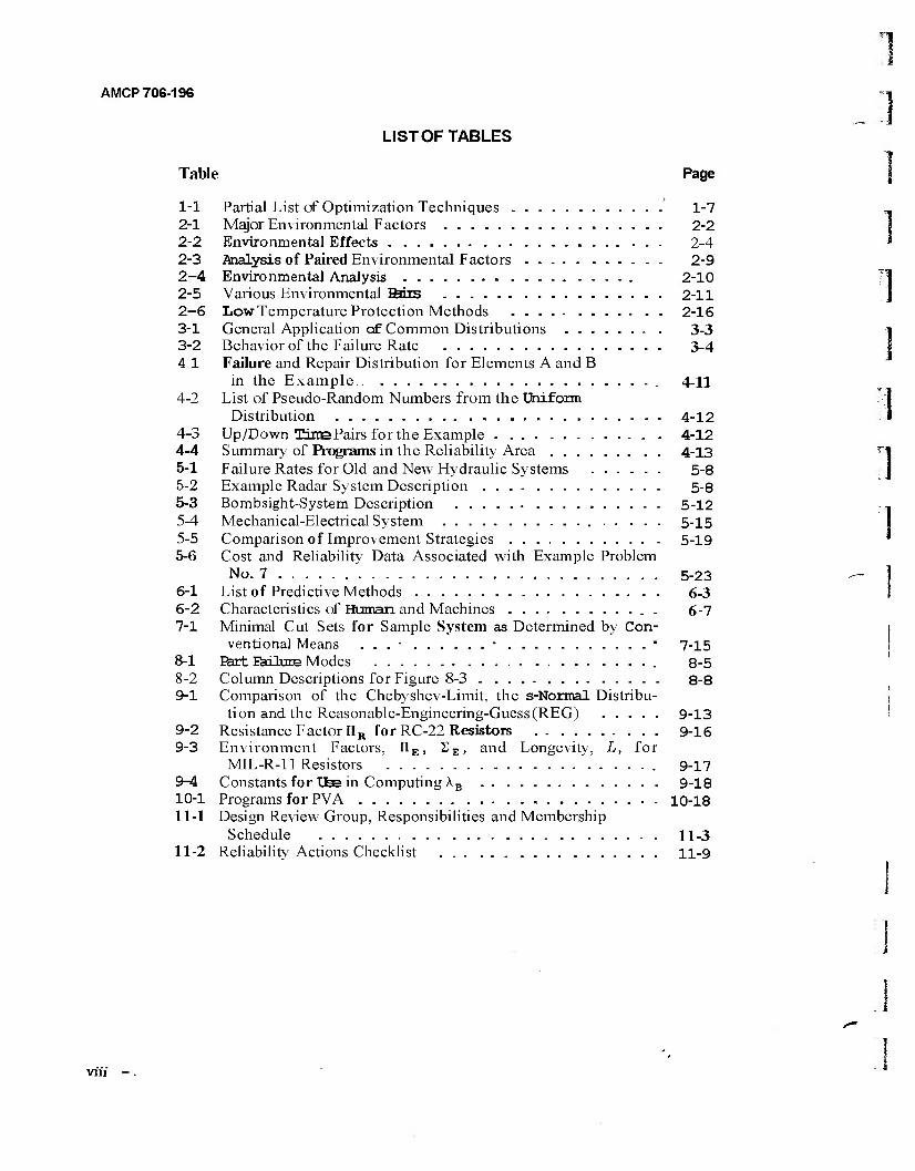
LIST OF TABLES

Table Page

1-1 Partial List cf Optimization Techniques 1-7 2-1 Major Environmental Factors 2-2 2-2 Environmental Effects 2-4 2-3 Analysis of Paired Environmental Factors 2-9 2-4 Environmental Analysis 2-10 2-5 Various Environmental Tfrirs 2-11 2-6 Low Temperature Protection Methods 2-16 3-1 General Application of Common Distributions 3-3 3-2 Behavior of the Failure Rate 3-4 4 1 Failure and Repair Distribution for Elements A and B

in the Example 4-H 4-2 List of Pseudo-Random Numbers from the Uniform

Distribution 4-12 4-3 Up/Down Time Pairs for the Example 4-12 4-4 Summary of Programs in the Reliability Area 4-13 5-1 Failure Rates for Old and New Hydraulic Systems 5-8 5-2 Example Radar System Description 5-8 5-3 Bombsight-System Description 5-12 5-4 Mechanical-Electrical System 5-15 5-5 Comparison of Improvement Strategies 5-19 5-6 Cost and Reliability Data Associated with Example Problem

No. 7 5-23 6-1 List of Predictive Methods 6-3 6-2 Characteristics of Human and Machines . 6-7 7-1 Minimal Cut Sets for Sample System as Determined by Con-

ventional Means . . . ■ ■ ■ 7-15 8-1 Eört Eailure Modes 8-5 8-2 Column Descriptions for Figure 8-3 8-8 9-1 Comparison of the Chebyshev-Limit, the s-Normal Distribu-

tion and the Reasonable-Engineering-Guess (REG) 9-13 9-2 Resistance Factor IIR for RC-22 Resistors 9-16 9-3 Environment Factors, F1E, £E, and Longevity, L, for

MIL-R-11 Resistors 9-17 9^4 Constants for Ute in Computing AB 9-18 10-1 Programs for PVA 10-18 11-1 Design Review Group, Responsibilities and Membership

Schedule 11-3 11-2 Reliability Actions Checklist 11-9

vni -

AMCP 706-196

PREFACE

This handbook, Design for Reliability is the first in a series of five on reliability. The series is directed largely toward the working engineers who have the responsibility for creating and producing equipment and systems which can be relied upon by the users in the field.

The five handbooks are:

1. Design for Reliability, AMCP 706-196 2. Reliability Prediction, AMCP 706-197 3. Reliability Measurement, AMCP 706-198 4. Contracting for Reliability, AMCP 706-199 5. Mathematical Appendix and Glossary, AMCP 706-200.

This handbook is directed toward reliability engineers who need to be familiar with the mathematical-probabilistic-statistical techniques for predicting the reliability of various configurations of hardware. The material in standard textbooks is not repeated here; the important points are summarized, and references are given to the standard works.

The majority of the handbook content was obtained from many individuals, reports, journals, books, and other literature. It is impractical here to acknowledge the assistance of everyone who made a contribution,

The original volume was prepared by Tracor Jitco, Inc. The revision was prepared by Dr. Ralph A. Evans of Evans Associates, Durham, N.C., for the Engineering Handbook Office of the Research Triangle Institute, prime contractor to the US Army Materiel Command. Technical guidance and coordination on the original draft were provided by a committee under the direction of Mr. O. P. Bruno, US Army Materiel Systems Analysis Agency, US Army Materiel Command.

The Engineering Design Handbooks fall into two basic categories, those approved for release and sale, and those classified for security reasons. The US Army Materiel Command policy is to release these Engineering Design Handbooks in accordance with current DOD Directive 7230.7, dated 18 September 1973. All unclassified handbooks can be obtained from the National Technical Information Service (NTIS). Procedures for acquiring these handbooks follow:

a. All Department of Army activities having need for the handbooks must submit their request on an official requisition form (DA Form 17, dated Jan 70) directly to:

Commander Uetterkenny Army Depot ATTN: AMXUE-ATD Chambersburg, PA 17201

(Requests for classified documents must be submitted, with appropriate "Need to Know" justification, to Uetterkenny Army Depot,) DA activities will not requisition handbooks for further free distribution.

IX

1 AMCP 706-196

b. AH other requestors, DOD, Navy, Air Force, Marine Corps, non- military Government agencies, contractors, private industry, individuals, universities, and others must purchase these handbooks from:

National Technical Information Service Department of Commerce Springfield, VA 22151

Classified documents may be released on a VNeed to Know" basis verified by an official Department of Army representative and processed from-Defense Documentation Center (DDC), ATTN: DDC-TSR, Cameron Station, Alexandria, VA 22314.

Comments and suggestions on this handbook are welcome and should be addressed to:

Commander US Army Materiel Development and Readiness Command Alexandria, VA 22333

(DA Forms 2028, Recommended Changes to Publications, which are available through normal publications supply channels, may be used for comments/suggestions. )

1 1 ]

AMCP 706-196

CHAPTER I INTRODUCTION

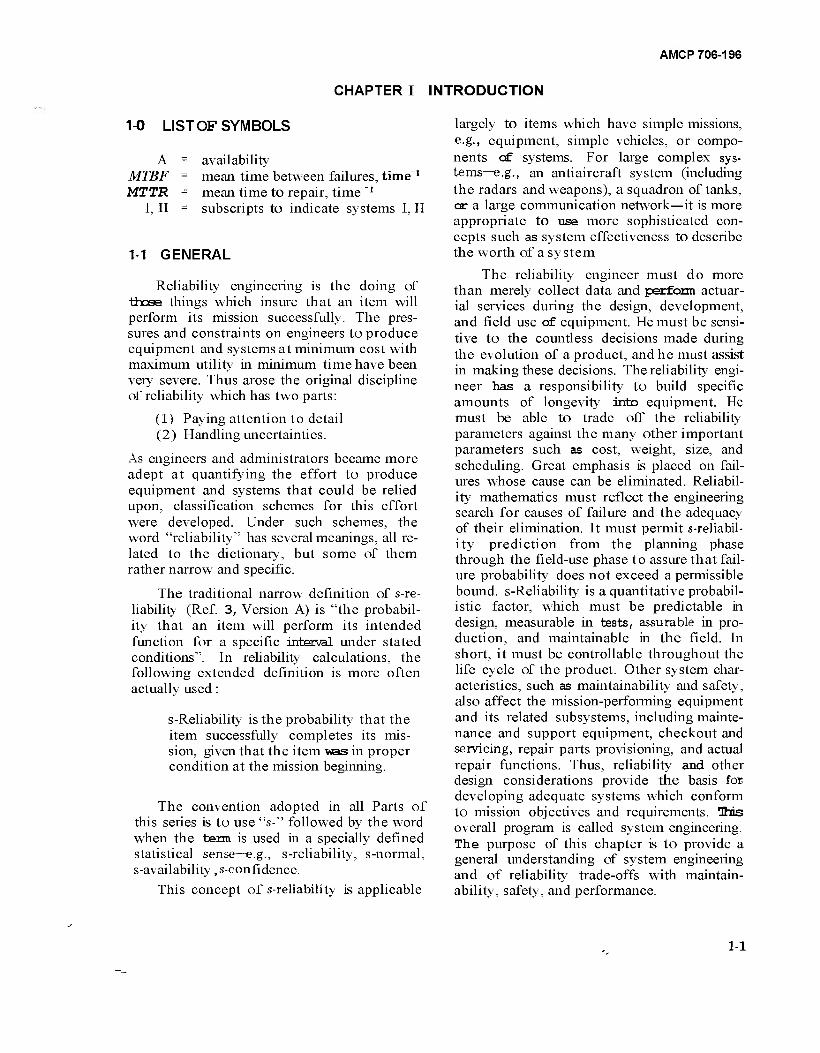
1-0 LIST OF SYMBOLS

A = availability MTBF - mean time between failures, time"1

MTTR = mean time to repair, time _1

I, II = subscripts to indicate systems I, II

1-1 GENERAL

Reliability engineering is the doing of those things which insure that an item will perform its mission successfully. The pressures and constraints on engineers to produce equipment and systems at minimum cost with maximum utility in minimum time have been very severe. Thus arose the original discipline of reliability which has two parts:

(1) Paying attention to detail (2) Handling uncertainties.

As engineers and administrators became more adept at quantifying the effort to produce equipment and systems that could be relied upon, classification schemes for this effort were developed. Under such schemes, the word "reliability" has several meanings, all related to the dictionary, but some of them rather narrow and specific.

The traditional narrow definition of s-reliability (Ref. 3, Version A) is "the probability that an item will perform its intended function for a specific interval under stated conditions". In reliability calculations, the following extended definition is more often actually used:

s-Reliability is the probability that the item successfully completes its mission, given that the item was in proper condition at the mission beginning.

The convention adopted in all Parts of this series is to use "s-" followed by the word when the term is used in a specially defined statistical sense—e.g., s-reliability, s-normal, s-availability ,s-confidence.

This concept of s-reliability is applicable

largely to items which have simple missions, e.g., equipment, simple vehicles, or components of systems. For large complex systems—e.g., an antiaircraft system (including the radars and weapons), a squadron of tanks, or a large communication network—it is more appropriate to use more sophisticated concepts such as system effectiveness to describe the worth of a system

The reliability engineer must do more than merely collect data and perform actuar- ial services during the design, development, and field use of equipment. He must be sensitive to the countless decisions made during the evolution of a product, and he must assist in making these decisions. The reliability engineer has a responsibility to build specific amounts of longevity into equipment. He must be able to trade off the reliability parameters against the many other important parameters such as cost, weight, size, and scheduling. Great emphasis is placed on failures whose cause can be eliminated. Reliabil- ity mathematics must reflect the engineering search for causes of failure and the adequacy of their elimination. It must permit s-reliability prediction from the planning phase through the field-use phase to assure that failure probability does not exceed a permissible bound. s-Reliability is a quantitative probabilistic factor, which must be predictable in design, measurable in tests, assurable in production, and maintainable in the field. In short, it must be controllable throughout the life cycle of the product. Other system characteristics, such as maintainability and safety, also affect the mission-performing equipment and its related subsystems, including maintenance and support equipment, checkout and servicing, repair parts provisioning, and actual repair functions. Thus, reliability and other design considerations provide the basis fo* developing adequate systems which conform to mission objectives and requirements. This overall program is called system engineering. The purpose of this chapter is to provide a general understanding of system engineering and of reliability trade-offs with maintainability, safety, and performance.

1-1

AMCP 706-196

1-2 SYSTEM ENGINEERING

In recent years, come to include:

the word system has

(1) The prime mission equipment (2) The facilities required for operation

and maintenance (3) The selection and training of per-

sonnel (4) Operational and maintenance pro-

cedures (5) Instrumentation and data reduction

for test and evaluation (6) Special activation and acceptance

programs (7) Logistic support programs.

Specifically, a system is defined (Ref. 1, Ver- sion A) as: "A composite, at any level of complexity, of operational and support equipment , personnel, facilities, and software which are used together as an entity and capable of performing and supporting an operational role".

System engineering (Ref. 2) is the application of scientific, engineering, and management effort to:

(1) Transform an operational need into a description of system performance parameters and a system configuration through theuse of an iterative process of definition, synthesis, analysis, design, test, and evaluation

(2) Integrate related technical parameters and assure compatibility of all physical, functional, and program interfaces in a manner that optimizes the total system design

(3) Integrate reliability, maintainability, safety, survivability (including electronic warfare considerations), human factors, and other factors into the total engineering effort.

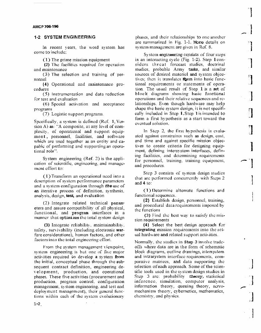
From the system management viewpoint, system engineering is but one of five major activities required to develop a system from the initial, conceptual phase through the subsequent contract definition, engineering development, production, and operational phases. These five activities (procurement and production, program control, configuration management, system engineering, and test and deployment management), their general functions within each of the system evolutionary

phases, and their relationships to one another are summarized in Fig. 1-1. More details on system management are given in Ref. 8.

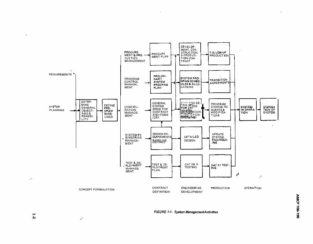
System engineering consists of four steps in an interacting cycle (Fig. 1-2). Step 1 considers threat forecast studies, doctrinal studies, probable Army tasks, and similar sources of desired materiel and system objectives; then it translates tjjem into basic functional requirements or statements of operation. The usual result of Step 1 is a set of block diagrams showing basic functional operations and their relative sequences and relationships. Even though hardware may help shape the basic system design, it is not specifically included in Step l.Step lis intended to form a first hypothesis as a start toward the eventual solution.

In Step 2, the first hypothesis is evaluated against constraints such as design, cost, and time and against specific mission objectives to create criteria for designing equipment, defining intersystem interfaces, defining facilities, and determining requirements for personnel, training, training equipment, and procedures.

Step 3 consists of system design studies that are performed concurrently with Steps 2 and 4 to:

(1) Determine alternate functions and functional sequences.

(2) Establish design, personnel, training, and procedural data requirements imposed by the functions

(3) Find the best way to satisfy the mission requirements

(4) Select the best design approach for integrating mission requirements into the actual hardware and related support activities.

Normally, the studies in Step 3 involve trade- offs where data are in the form of schematic block diagrams, outline drawings, intersystem and intrasystem interface requirements, comparative matrices, and data supporting the selection of each approach. Some of the scientific tools used in the system design studies in Step 3 are: probability theory, statistical inference, simulation, computer analysis, information theory, queuing theory, servo- mechanism theory, cybernetics, mathematics, chemistry, and physics.

!1

1-2

REQUIREMENT6

SYSTEM PLANNING

DETER- MINE GENERAL OBJECT- IVES & FEASIBI- LITY

DEFINE PRO- GRAM BASE- LINES

PROCURE- MENTS! PRO- - DUCTION MANAGEMENT

PROGRAM CONTROL MANAGE. MENT

CONFIGU- RATION MANAGE- MENT

SYSTEM EN- GINEERING MANAGE- MENT

TEST & DE- PLOYMENT MANAGE- MENT

PROCURE- MENT PLAN

PRELIMI- NARY SYSTEM PROGRAM PLAN

DEVELOP- MENT, CON- STRUCTION, & PRODUC- TION CON. TRACT

GENERAL SYSTEM SPECS FOR CONTRACT END ITEMS ICED

SYSTEM PRO- GRAM SCHED- ULES & ALLO- CATIONS

DESIGN RE QUIREMENTS

t»TS

D DE

FOR CE CON

..._, ....ION lÄSIblNEI

L

DETAILED DESIGN

FOLLOW-UP PRODUCTION

TRANSITION AGREEMENTS

t- PROGRAM CHANGE RE- QUESTS & MODIFICA- TIONS

UPDATE SYSTEM ENGINEER- ING

TEST& DE- PLOYMENT PLAN

CAT 1 & 11 TESTING

CAT III TEST- ING

SYSTEM IN OPERA- TION

DISPOSI- TION OF SYSTEM

CONCEPT FORMULATION CONTRACT DEFINITION

ENGINEERING DEVELOPMENT

PRODUCTION OPERATION

FIGURE 1-1. System Management Activities

Co

> S o

o

s

AMCP 706-196

STEP 1 . . — STFP^> STPD A

TRANSLATE SYSTEM REQUIREMENTS INTO FUNCTIONAL REQUIRE- MENTS

ANALYZE FUNCTIONS & TRANSLATE INTO RE- QUIREMENTS FOR 0€- SIGN, FACILITIES, PER- SONNEL, TRAINING, AND PROCEDURES

INTEGRATE REQUIRE- MENTS INTO CONTRACT END ITEMS, TRAINING, & TECHNICAL PROCE- DURES

1 i I

I i *

1

1 1

i

—*

STEP 3

1

SYSTEM/DESIGN ENGI- NEERING TRADE-OFF STUDIES TO DETERMINE REQUIREMENTS AND DESIGN APPROACH 1

FIGURE 1-2. Fundamental System Engineering Process Cycle

Step 4 uses the design approach selected in Step 3 to integrate the design requirements from Step 2 into the Contract End Items (CEI's). The result of Step 4 provides the criteria for detailed design, development, and test of the CEI based upon defined engineering information and associated tolerances. Outputs from Step 4 are used to:

(1) Determine intersystem interfaces (2) Formulate additional requirements

and functions that evolve from the selected devices or techniques

(3) Provide feedback to modify or verify the system requirements and functional flow diagrams prepared in Step 1.

When the first cycle of the system engineering process is completed, the modifications, alternatives, imposed constraints, additional requirements, and technological problems that have been identified are recycled through the process with the original hypothesis (initial design) to make the design more practical. This cycling is continued until a satisfactory design is produced, or until available resources (time, money, etc.) are expend- ed and the existing design is accepted, or until the objectives are found to be unattainable.

1-4 -

Other factors that are part of thesystem engineering process—such as reliability, maintainability, safety, and human factors—exist as separate but interacting engineering disciplines and provide specific inputs to each other and to the overall system program. Per- tinent questions at this point might be: "How do we know when the design is adequate?" or "How is the effectiveness of a system measured?" The answers to these questions lead to the concept of system effectiveness.

1-3 SYSTEM EFFECTIVENESS

System effectiveness is defined (Ref. 3, Version B) as: "a measure of the degree to which an item can be expected to achieve a set of specific mission requirements, and which may be expressed as a function of availability, dependability, and capability". Cost and time are also critical in the evaluation of the merits of a system or its components and must eventually be included in making administrative decisions regarding the purchase, use, maintenance, or discard of any equipment.

The effectiveness of a system obviously is influenced by the way the equipment was designed and built, it is. however, just as

AMCP 706-196

influenced by the way the equipment is used and maintained; i.e., system effectiveness is influenced by the designer, production engineer, maintenance man, and user/operator. The concepts of availability, dependability, and capability included in the definition of system effectiveness illustrate these influences and their relationships to system effectiveness. MIL-STD-721 (Ref. 3, Version B) provides the following definitions of these concepts:

(1) Availability. A measure of the degree to which an item is in an operable and com- mittable state at the start of a mission, when the mission is called for at an unknown (randomj point in time.

(2) Dependability. A measure of the item operating condition at one or more points during the mission, including the effects of reliability, maintainability, and survivability, given the item condition(s) at the start of the mission. It may be stated as the probability that an item will: (a) enter or occupy any one of its required operational modes during a specified mission, and (b) perform the functions associated with these operational modes.

(3) Capability. A measure of the ability of an item to achieve mission objectives, given the conditions during the mission.

Dependability is related to reliability; the intention was that dependability would be a more general concept than reliability. No designer should become bogged down in semantic discussions when intent is clear.

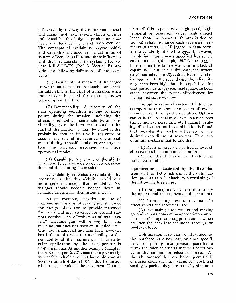
As an example, consider the use of machine guns against attacking aircraft. Since the design intent was to provide increased firepower and area coverage for ground support combat, the effectiveness of this "system" (machine gun) will be very low. The machine gun does not have an intended capability for antiaircraft use. This fact, however, has little to do with the availability or dependability of the machine gun. That particular application by the user/operator is simply a misuse. As another example (adapted from Ref. 4, par. 2.7.3), consider a previously serviceable vehicle tire that has a blowout at 90 mph on a hot day (110"F) due to impact with a jagged hole in the pavement. If most

tires of this type survive high-speed, high- temperature operation under high impact loads, then the blowout (failure) is due to lack cf reliability, since such severe environments (90 mph, 110° F, jagged hole) are within the capability of the tire type. If, however, the design requirements specified less severe environments (60 mph, 80° F, no jagged holes), then the failure was due to a lack of capability. Thus, in the first case, the system (tire) had adequate capability, but its reliability VBS low. In the second case, the reliability may have been high, but the capability (for that particular usage) was inadequate. In both cases, however, the system effectiveness for the applied usage was low.

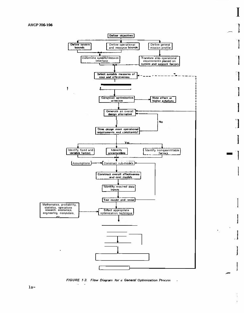
The optimization of system effectiveness is important throughout the system life cycle, frcm concept through the operation. Optimi- zation is the balancing of available resources (time, money, personnel, etc.) against resulting effectiveness, until a combination is found that provides the most effectiveness for the desired expenditure of resources. Thus, the optimum system might be one that:

(1) Meets or exceeds a particular level of effectiveness for minimum cost, and/or

(2) Provides a maximum effectiveness for a given total cost.

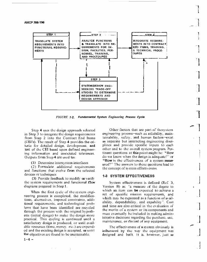
Optimization is illustrated by the flow diagram of Fig. 1-3 which shows the optimization process as a feedback loop consisting of the following three steps:

(1) Designing many systems that satisfy the operational requirements and constraints.

(2) Computing resultant values for effectiveness and resources used

(3) Evaluating these results and making generalizations concerning appropriate combinations of design and support factors, which are then fed back into the model through the feedback loops.

Optimization also can be illustrated by the purchase of a new car, or more specifically, of putting into precise, quantifiable terms the rules or criteria that will be followed in the automobile selection process- Al- though automobiles do have quantifiable characteristics, such as horsepower, cost, and seating capacity, they are basically similar in

1-5

I AMCP 706-196

| Define objectives |

Define system bounds

Define operational and resource bounds

Define general mission profile

Determine system/resource Interface

Translate into operational requirements placed on

system and support factors

Select suitable measures of cost and effectiveness

Construct optimization criterion

Generate an overall design alternative

Does design meet operational requirements and constraints?

IdenfiTy fixed and variable factors

T

Yes

Identity uncertainties

F [Assumptions | »{construct sub-modelsJ»

Construct overall effectiveness and cost models

IdenfiTy required data inputs

Mathematics, probability, statistics, operations research, economics,

engineering, computers, etc,

j Test model and revise (-

Select appropriate optimization technique

Note effect at higher echelons

No

IdenfiTy nonq.uantifiable factors

FIGURE 1-3. Flow Diagram for a General Optimization Process

la-

AMCP 706-196

most cars of a particular class (low-price sedans, sports models, etc.)- Thus, the selection criteria essentially reduce to esthetic appeal, prior experience with particular models, and similar intangibles. In the same sense, the choice of best design for the weapon system is greatly influenced by experience with good engineering practices, knowledge assimilated from similar systems, and economics. Despite this fuzziness, the selection criteria must be adjusted so that:

(l)The problem size can be reduced to ease the choice of approaches

(2) All possible alternatives can be examined more readily and objectively for adapta- tion to mathematical representation and analysis

(3) Ideas and experiences frcm other disciplines can be more easily incorporated into the solution

(4) The final choice of design approaches can be based on more precise, quantifiable terms, permitting more effective review and revision, and better inputs for future optimization problems.

The choice of parameters in the optimization model also is influenced by system definition. The automobile purchaser, for example, may not consider the manufacturer's and dealer's service policies. If these policies are considered, the system becomes the automobile plus the sendee policies. If service policies are not considered, the system consists only of the autanobile.

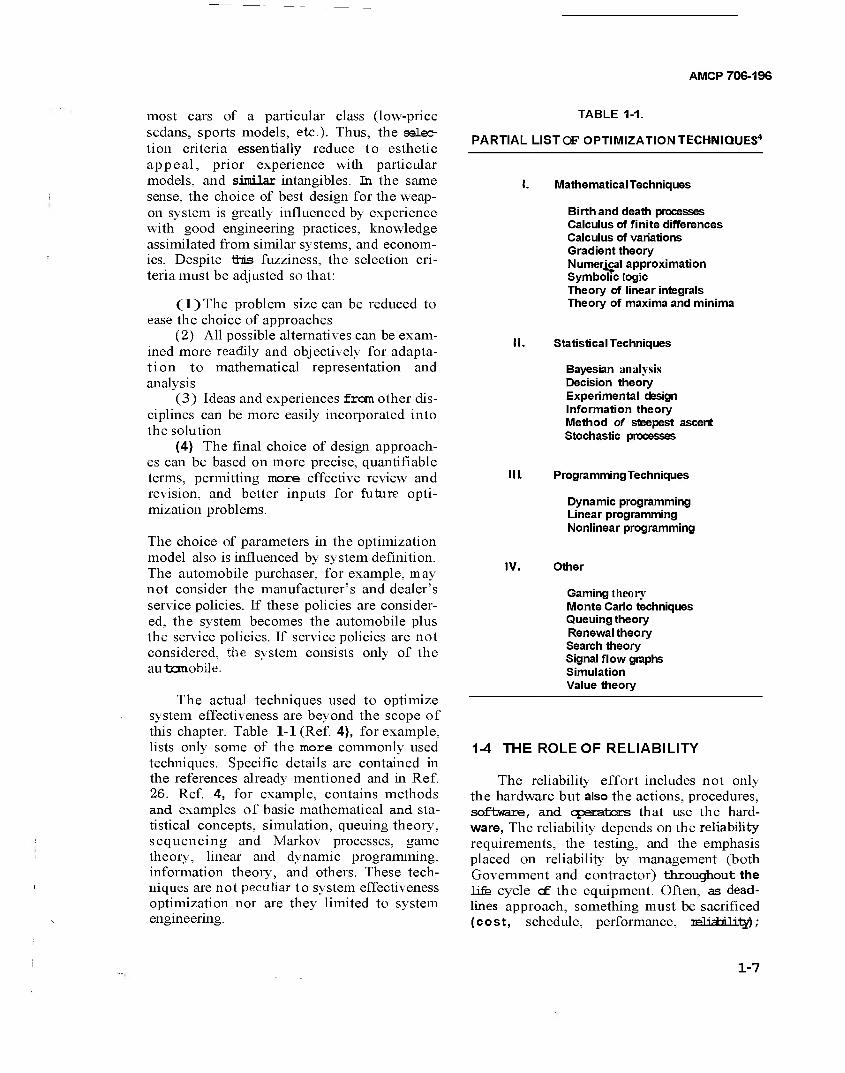
The actual techniques used to optimize system effectiveness are beyond the scope of this chapter. Table 1-1 (Ref. 4), for example, lists only some of the more commonly used techniques. Specific details are contained in the references already mentioned and in Ref. 26. Ref. 4, for example, contains methods and examples of basic mathematical and statistical concepts, simulation, queuing theory, sequencing and Markov processes, game theory, linear and dynamic programming, information theory, and others. These techniques are not peculiar to system effectiveness optimization nor are they limited to system engineering.

TABLE 1-1.

PARTIAL LIST OF OPTIMIZATION TECHNIQUES4

Mathematical Techniques

Birth and death processes Calculus of finite differences Calculus of variations Gradient theory Numerjcal approximation Symbolic logic Theory of linear integrals Theory of maxima and minima

Statistical Techniques

Bayesian analysis Decision theory Experimental design Information theory Method of steepest ascent Stochastic processes

ML Programming Techniques

Dynamic programming Linear programming Nonlinear programming

IV. Other

Gaming theory Monte Carlo techniques Queuing theory Renewal theory Search theory Signal flow graphs Simulation Value theory

1-4 THE ROLE OF RELIABILITY

The reliability effort includes not only the hardware but also the actions, procedures, software, and operators that use the hardware, The reliability depends on the reliability requirements, the testing, and the emphasis placed on reliability by management (both Government and contractor) throughout the life cycle cf the equipment. Often, as dead- lines approach, something must be sacrificed (cost, schedule, performance, TPlirJ-rility);

1-7

AMCP 706-196

management decides what it will be; e.g., will management decide that a paper "demonstration" be substituted for a physical demonstration rFra\ iîlity?

It is much easier to talk about optimizing reliability and to analyze ways of doing it than it is to get a physical system which is optimized. Achieving high reliability is an engineering problem, not a statistical one.

Before reliability can be optimized, one needs to look at ways reliability can be changed and the kinds of constraints that can be imposed upon efforts to change it. These classifications are convenient for discussion. They do not in themselves limit anyone's activities. Not all changes which are made with the intention of improving reliability actually do improve it—especially when there is insufficient information about the mission.

Reliability can be modified by changing:

(1) The overall approach to the problem (e.g., wire lines or a microwave link for a communication system)

(2) The configuration of the system (e.g., an aircraft can have propeller or jet engines, wings over or under the fuselage, and the mounting and number of engines are adjustable)

(3) Some of the modules or subsystems (e.g., motor functions can be performed electrically, hydraulically, or by mechanical levers and gears)

(4) Some components (e.g., use high reliability parts or commercial ones)

(5) Details of manufacture (e.g., holes in steel can be punched, drilled, reamed, and/or burned)

(6) Materials (e.g., wood, plastics, metal alloys)

(7) Method of operation (e.g., the operator of a radio-receiver can be required to tune each stage separately or it can all be done with one switch)

(8) Definition of mission success (e.g., range and resolution of a radar)

(9) Amount of attention to detail (e.g., an alloy can simply be selected from a handbook table, or many tests can be run on many alloys to find the one which holds up best in service).

Efforts to improve reliability are constrained by:

(1) Cost of design effort (2) Cost of parts manufacture (3) Calendar time schedules (4) Manpower available to do the job (5) Availability of purchased compo-

nents or materials (6) Volume or weigrk of finished prod-

uct (7) Operator training limitations (8) Uncertainty about actual use condi-

tions (9) Maintenance philosophy, and logis-

tics (10) Logical consequences of various

user regulations (11) User resistance to some configura-

tions (12) Management refusal to effect ad-

ministrative changes (13) Lack of knowledge about material

or component properties or about the way a part will be made.

Other techniques and constraints are likely tobe important in any particular job. Some of the changes and constraints are not easily quantifiable, and the ones listed are certainly not mutually exclusive. All of this makes a complete mathematical analysis virtually impossible.

It is worthwhile to have many of the critical failure modes such that the equipment fails gracefully; viz., there is a very degraded mode of operation which is still feasible after the major failure. For example, if the power steering on a vehicle fails, it may still be possible for it to limp to safety if thevehicle can be steered by hand.

The repair philosophy during a mission must be stated explicitly- Standby redundancy often can be considered a special case of repair—it is just a question of how the changeover is effected in case of failure. In some situations, the mission will not be a failure if the equipment is down for only a very short time. In what state will a repair leave the system'! Is the entire system to be restored to a like-new condition after each failure? Will only a subsystem be restored to like-new or perhaps the equipment will be

1-8

AMCP 706-196

returned to the statistical condition it had just before failure? In general, the exact situation will not be known, and it is a matter of engineering judgment to pick tractable assumptions that are reasonably realistic.

The design approaches and requirements are investigated by the system reliability engineer. They include the following:

(l)The definitions of (a) the mission, (b) successful completion, and (c) proper condition (at mission beginning) must be sufficiently explicit to make the reliability calculations.

(2) Relationships and interactions between reliability and each of the other system parameters (maintainability, etc.) must be carefully analyzed.

(3) A method of estimating reliability must be selected to permit quantitative description of the consequences of each design.

(4) Reliability objectives must be match- ed to the system mission.

(5) System reliability levels must be related to overall program resource allocations.

These and others are discussed in this handbook and Parts Three, Four, and Five.

The techniques used in this analysis include development of a model that considers :

(1) Required functions for each mission phase

(2) Identification of critical time periods for each function

(3) Establishment of external and internal environmental stresses for each functional element

(4) Operational and maintenance concepts

(5) Hardware and software system elements for each function

(6) Determination of any required functional redundancies.

Specific design techniques, such as stress derating, redundancy, stressj strength analysis, apportionment of reliability requirements, prediction, design of experiments and tests, parameter variation analysis, failure mode and effect analysis, and worst case analysis, are the "tools c£ the trade" for reliability engineers. Additionally, the reliability engineer must:

(1) Actively participate in selecting preferred parts having established reliabilities, and thus promote standardization within military system.

(2) Participate in design reviews at appropriate stages "to evaluate reliability objectives and achievement thereof.

(3) Monitor attainment of reliability requirements throughout the entire program.

(4) Work with other members of the system engrneering~-team to integrate reliability with other engineering areas.

Thus, the reliability engineer performs system engineering fron the reliability viewpoint. These methods and techniques are discussed in greater detail in later chapters and other Parts. Additional information is provided in the references at the end of this chapter; e.g., MIL-STD-785 (Ref. l)specifies the requirements for system reliability programs, MIL STD-721 (Ref. 3) defines terms for reliability and related disciplines, and AR 702-3 (Ref. 5) establishes Army requirements for reliability and maintainability.

1-5 THE ROLE OF MAINTAINABILITY

Maintainability is a characteristic of design and installation of equipment. s-Maintain- ability is defined (Ref. 3) as the probability that an item will be retained in a specified condition, or restored to that condition within a given time period, when maintenance is performed according to prescribed procedures and resources. Maintenance consists of those actions needed to retain the designed-in characteristics throughout the sysban lifetime. Maintainability, like reliability, must be designed into the equipment.

Maintainability engineering is similar to other engineering practices, but it emphasizes recovery of the equipment after a failure and reductions in upkeep costs. Maintainability engineers consider the purpose, type, use, and limitations of the product, all of which influence the ease, rapidity, economy, accuracy of its service and repair, effects of installation, environment, support equipment, personnel, and operational policies on the item geometry, size, and weight. Thus, maintainability studies assist in the development of a product which can be maintained by personnel of

1-9

AMCP 706-196

ordinary skill under the environmental conditions in which it will operate.

1-5.1 RELATIONSHIP TO RELIABILITY

Reliability is related to the effectiveness of the maintenance perfoxmed on a system. If this maintenance is incorrect or not timely, the system may fail- Maintainability, on the other hand, can provide designed-in ease of maintenance and, thereby, increase the maintenance effectiveness.

Fccm a system effectiveness viewpoint, reliability and maintainability j ointly provide system availability and dependability. Increas- ed reliability directly contributes to system uptime, while improved maintainability reduces downtime. If reliäaLLüy and maintainability are not jointly considered and con- tiiually reviewed, as required by Ref. 5, then serious consequences may result. With military equipment, failures or excessive downtime can jeopardize a mission and possibly cause a loss of lives. Excessive repair time and failures also impose burdens on logistic support and maintenance activities, causing high costs for repair parts and personnel training, expenditure of many man-hours for actual repair and sendee, obligation of facilities and equipment to test and service, and to movement and storage of repair parts.

From the cost viewpoint, reliability and maintainability must be evaluated over the system life cycle, rather then merely from the standpoint of initial acquisition. The overall cost of ownership has been estimated to be from three to twenty times the original acquisition cost. An effective design approach to reliability and maintainability can reduce this cost of upkeep.

The reliability and maintainability characteristics of an item are relatively fixBd and difficult to change in the field. Thus, the soldier/user finds himself faced with accepting the item reliability as a determination of whether the item* will function correctly or not; as long as it functions, he can use it. Consequently, reliability data do not greatly concern him (Ref, 7). Maintainability, on the other hand, provides the soldier/user with his only means of returning the equipment to a serviceable condition, A tank, for example,

that has a nonrepairable weapon system beccmes, on breakdown of the weapon, an immensely heavy mobile radio from the viewpoint of its users.

The primary objectives of the Army reliability , availability, and maintainability (RAM) programs are to assure that Army materiel will:

(1) Be ready foruse When needed (2) Be capable of successfully complet-

ing its mission and (3) HJLELU aU required maintenance ob-

jectives throughout its life cycle.

Ref. 8 provides guidance on management of reliability and maintainability programs, and Ref. 5 delineates concepts, objectives, responsibilities, and general policies for Army reliability and maintainability programs.

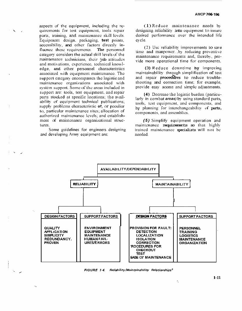
Policies and guidance on life cycles of Army equipment are provided by Refs. 6 and 9. Amplification of Army reliability and maintainability policies can be found in the references at the end of this chapter. Fig. 1-4 illustrates some of the fundamental relationships between reliability and maintainability.

1-5.2 DESIGN GUIDELINES

System maintainability goals must be apportioned among three major categories: (1) equipment design, (2) personnel, and (3)

support. To accomplish this, a maintenance concept must be selected, and a mathematical model developed to describe the concept. Initially, the goals can be apportioned based upon past experience with similar systems, and upon general guidelines presented here and in the references for this chapter. As the design progresses, the initial apportionment can be changed by trade-offs among these three categories. The design goals can be further apportioned to the subsystem and component levels. Allocating maintainability for subsystems and components of a complex system can be difficult due to the mathematical/statistical complexity of the model. Some of the problems associated with combining or apportioning downtime and suggested approaches to their solution are covered in Refs. 7, 10,11, and 12.

The design category covers the physical

1-10-

AMCP 706-196

aspects of the equipment, including the requirements for test equipment, tools repair parts, training, and maintenance skill levels. Equipment design, packaging, test points, accessibility, and other factors directly influence these requirements. The personnel category considers the actual skill levels cf the maintenance technicians, their job attitudes and motivations, experience, technical knowledge, and other personnel characteristics associated with equipment maintenance. The support category encompasses the logistic and maintenance organizations associated with system support. Some of the areas included in support are: tools, test equipment, and repair parts stocked at specific locations; the availability of equipment technical publications; supply problems characteristic of, or peculiar to, particular maintenance sites; allocation of authorized maintenance levels; and establishment of maintenance organizational structures.

Some guidelines for engineers designing and developing Army equipment are:

(1) Reduce maintenance needs by designing reliability into equipment to insure desired performance over the intended life cycle.

(2) Use reliability improvements to save time and manpower. ,by reducing preventive maintenance requirements and, thereby, provide more operational time for components.

(3) Reduce downtime by improving maintainability through simplification of test and repair procedures to reduce troubleshooting and correction time; for example, provide easy access and simple adjustments.

(4) Decrease the logistic burden (particularly in combat areas) by using standard parts, tools, test equipment, and components, and by planning for interchangeability of parts, components, and assemblies.

(5) Simplify equipment operation and maintenance requrrari3T.ts so that highly trained maintenance specialists will not be needed.

AVAILABILITY/DEPENDABILITY

i

RELIABILITY

DESIGN FACTORS SUPPORTFACTORS

QUALITY APPLICATION SIMPLICITY REDUNDANCY. PROVEN

ENVIRONMENT EQUIPMENT MAINTENANCE HUMAN FAIL- URES/ERRORS

MAINTAINABILITY

DESIGN FACTORS

PROVISION FOR FAULT:

SUPPORT FACTORS

PERSONNEL DETECTION TRAINING LOCALIZATION LOGISTICS ISOLATION MAINTENANCE CORRECTION ORGANIZATION

■ROCEDURES FOR CHECKOUT TEST

EASE OF MAINTENANCE

FIGURE 1-4. Reliability/Maintainability Relationships1

1-11

AMCP 706-196

1-5.3 PREDICTION

M1it=ny specifications and contractual requirements incorporate maintenance time restrictions that must be met by the designer. Thus, predictions are needed to establish how close the equipment will be to these requirements during its development cycle and in its end-use phase. Similarly, a prediction of how long an item will be inoperative during maintenance is important to the user, because the user is deprived of the equipment contribution to his irdssicn performance. This prediction must be quantitative and be capable of being updated as the item progresses through successive development phases. Two advantages of predicting maintainability are that:

(1) It identifies areas of poor maintainability which must be improved.

(2) An early assessment can be made of the adequacy of predicted downtime, quality and quantity of maintenance and support personnel, and tools and test equipment.

Most maintainability prediction methods use recorded reliability and maintainability experience obtained from comparable systems and components under similar conditions of use and operation. Thus, it is common to assume that the principle-of-transferability is applicable. Basically, this principle is that data from a system can be transferred and used to predict the maintainability of a comparable system that is in the design, development, or evaluation phase. Obviously, this approach depends upon establishing some commonality between systems. Usually this commonality can be inferred on a broad basis during the early design phase; but as the design is refin- ed, the commonality must be established more exactly for equipment functions, maintenance task times, and levels of maintenance..

The data used in maintainability predictions depend on specific applications, but, in general, prediction methods use at least the following two parameters:

(1) Failure rates of components at the specific level of interest

(2) The amount of repair time required at each maintenance level-

A Repair times are obtained from prior experience, simulation of repair tasks, or data from similar applications on other systems. Component failure rates, however, have been recorded by many sources as a function of use and environment. Some of these sources are listed in Refs. 13-17, and in Appendix B. Actual prediction techniques are covered in detail in R=fe. 7, 10, 11, and 12.

1-5.4 DESIGN REVIEW

The design review process originally was established to achieve reliability objectives, but has since been extended to include all system characteristics throughout the life cycle (see Chap. 11).Maintainability specifications require that a formal design review program be established and documented for eacb development.

A design review involves four major tasks: (l)assembling data, (2) actual review, (3) documentation, and (4) followup. For maintainability, the first task (assembling data) includes engineering drawings: mock- ups, breadboard assemblies, or prototypes; maintainability prediction data; maintainability test data; and a description of the maintenance concept.

The review ought to be performed by people familiar with maintainability theory, maintenance processes, and human factors. The quantitative review techniques use prediction data to identify areas needing improvement, and the qualitative techniques use the experience and knowledge of the review board members, plus available reference material. The review ought to impartially analyze a design, isolate real or potential maintainability difficulties, propose solutions, and document the proceedings so that the designer can incorporate any needed changes. Thus, the designer benefits from the experience of other technical disciplines, and the equipment is improved. Design review meetings must be held at each stage during the equipment development to exercise control over the design, and to allow easier incorporation of changes. Further discussion of reviews is in Chapter 11.

1

3

1

1-12

AMCP 706-196

1-5.5 AVAILABILITY

Maintainability trade-off techniques are used by designers to weigh the potential advantages of a maintainability design change against possible disadvantages. If mission requirements allow it, trade-offs can be made between maintainability and other parameters, such as reliability, or among the three categories of maintainability equipment—i.e., design, personnel, and support.

Availability is one of the important characteristics of equipment and systems. Gen- erally speaking, s-availability is said to be the probability that, at any instant, an item is in proper condition to begin a mission (see the second definition of s-reliability in par. 1-1). There are many variations for an exact definition (see Ref. 10); they usually explicitly state what kinds of downtime are to be excluded or included in the calculation. Ref. 10 ought to be consulted for formal definitions of s-availability; for the purposes of this paragraph s-availability will be taken as

A = 1/[1 + (MTTR/MTBF)) (l-i)

where A = availability calculated without

considering downtime for scheduled or preventive maintenance, or logistic support. Ready time, supply downtime, waiting or administrative downtime, and preventive maintenance downtime are all excluded (see Ref. 10 for definitions).

MTBF = Mean Time Between Failures, ignoring downtime.

MTTR = Mean Time To Repair, viz., the average time required to detect and isolate a malfunction, make repairs, and restore the system to satisfactory performance (see the definition of A for other conditions)-

s-Availability can be improved by reducing MTTR and by increasing MTBF. Either MTTR = 0 or MTBF -* °° would provide per- fect s-availability but, of course, neither is possible.

As examples, consider systems I and II with

MTTR, =0.1hr MTBF, = 2 hr MTTRn =10hr

MTBF, , = 200 hr

Then the s-availability is

A, = 1/[1 + (0.1/2)] = 0.952 (l-2a) An = 1/[1 + (10/200)] = 0.952 (l-2b)

Both systems have the same s-availability, but they are not equally desirable. A 10-hr MTTR might be too long for some systems whereas a 2-hr MTBF might be too short for some systems.

Even though reliability and maintainability individually can be increased or decreased in combinations giving the same system availability, care must be taken to insure that reliability does not fall below its specified minimum, or that individually acceptable values of reliability and maintainability are not combined to produce an unacceptable level of system availability.

Other trade-off techniques involve:

(1) Increasing system availability by improving maintainability through trade-offs between design and support parameters, for example, by using sophisticated maintenance equipment to reduce maintainability requirements. This method, however, may increase overall program costs.

(2) Comparing costs versus availability for a basic system, a redundant system, a basic system plus sophisticated support equipment, etc., to determine which approach provides the highest availability for the least cost.

(3) Extending system-level techniques to subsystem or component levels and then working upward to the overall system level.

Refs. 7, 10, 11, and others at the end of this chapter provide additional discussions of trade-off techniques.

1-6 THE ROLE OF SAFETY

A safety program, one of the basic elements of the system engineering effort, has the following objectives:

1-13

AMCP 706-196

(1) Systan design must include a level of safety consistent with mission requirements.

(2) Hazards associated with each system, subsystem, and equipment must be identified, evaluated, and eliminated or controlled to an acceptable level.

(3) Hazards tha: cannot be eliminated must be controlled to protect personnel, equipment, and property.

(4) Minimum risk levels must be determined and applied in the acceptance and use of new materials, and new production and testing techniques.

(5) Retrofit actions required to improve safety must be minimized by conservative design during the acquisition of a system,

(6) Historical safety data generated by similar system programs must be considered and used where appropriate (Ref. 18).

The purpose of safety analysis is to identify hazards and minimize or eliminate risks. Statistical and analy'' ic techniques, however, are not a replacement for common sense. Sometimes, establishment of an acceptable risk level can result in unnecessary hazarHc when a change with a slight, acceptable increase in cost cur decrease in effectiveness would eliminate the risk entirely. This reasoning is particularly pertinent when the event, even though its probability of Occurrence is relatively low, might cause system failure.

1-6.1 RELATIONSHIPS TO RELIABILITY

Safety, like reliability and other system parameters, can be expressed as a probability, as, for example, the probability that no unsafe event will happen under specified operating conditions for a given time period. Thus, safety-analysis techniques closely parallel and, in some cases, actually use methods commonly associated with reliability. The Failure Mode and Effect Analysis (FMEA) and Cause-Consequence chart, for example, are reliability and safety tools. They are discussed in detail in Chapters 7 and 8. In general, safety is a specialized form of reliability study. This does not imply, however, that safety is a subordinate activity or derived discipline of reliability, but only that the activities of safety and reliability are closely related, both in concepts and in techniques. A system that is unreliable, for example, also

may be unsafe, because system failures may cause injuries or loss of life of operators or users.

People are a more important part of safety than of reliability, because of possible injury to users or bystanders even when the mission is not imperiled. The human subsystem is discussed further in Chapter 6.

Just as a reliability/maintainability guideline requires that components that are difficult to maintain should be made more reliable, a reliability/safety guideline requires increased reliability of components that are unsafe to repair or replace. Some additional safety guidelines and techniques are discussed in the paragraphs that follow. Their relationships to reliability and to system engineering produce data that are useful to these other disciplines and, similarly, allow use of information generated by studies performed by other technical fields.

1-6.2 SYSTEM HAZARD ANALYSIS

As shown in Fig. 1-1, system lifetime is divided into five phases: (l)concept formulation, (2) contract definition, (3) engineering development, (4) production, and (5) operation. During the concept formulation phase, a preliminary hazard analysis identifies potential hazards associated with each design and must be reviewed and revised as the system progresses through subsequent phases. This analysis is qualitative and develops safety criteria for inclusion in the performance and design specifications formulated in Step 2 of the system engineering process (par. 1-2). The preliminary hazard analysis also must consider solutions to safety problems, outline inade- quately defined conditions for additional study, and consider specific technical risks in the proposed design.

The subsystem hazard analysis is basically an expansion of the preliminary hazard analysis and usually occurs in the contract definition phase. Its purpose is to analyze the functional relationships between components of each subsystem and identify potential hazards due to component malfunctions or failures. Thus, the subsystem hazard analysis is similar to Step 3 of the system engineering process (par. 1 -2) and, in fact, provides inputs to Step

3

1-14

AMCP 706-196

3. An FMEA and Cause-Consequence chart, s adapted to the safety viewpoint, are included

to evaluate individual component failures and their influences on safety within each subsystem.

The contract definition phase also includes the system hazard analysis, which is basically an extension of the subsystem analysis in that the system hazard analysis treats safety integration and subsystem interfaces on an overall svstem basis. Trade-off and interaction studies during this phase must interlock with the system hazard analysis to obtain maximum system effectiveness and balanced apportionment among the various contributing disciplines (safety, reliability, etc.).

The operating hazard analysis encompasses safety requirements for personnel, procedures, and equipment in such functional areas as installation, maintenance, support, testing, storage, transportation, operation, training, and related activities. This study, like the previous ones, must be continued by reviews and revisions throughout the system life cycle, and involves having other disciplines (reliability, human factors, etc.) work with

•"' the safety engineers.

Thus, hazard analysis, through a comprehensive safety program, provides many useful inputs to the system engineering process and to other system parameters. These inputs—if effectively developed and intelligently used- can reduce overall program costs, contribute to economical scheduling, and make the task of interaction and trade-off studies much easier, since safety analysis techniques parallel or duplicate studies in reliability, maintainability, human factors, and other system disciplines.

1-6.3 TRADE-OFFS

Some trade-offs have been mentioned previously. The increase in reliability of parts that are relatively unsafe to repair or replace represents one such consideration. Trade-offs must be treated in the initial design phases, so that changes can be made early to preclude later problems in costs and scheduling or bare- ly adequate fixes.

The selection of trade-off alternatives

basically involves an analysis of all possible methods to improve safety, and a determination of the degree to which each method should be used. The analysis involves the investigation of safety hazards due to poor design, assembly errors, incorrect materials, improper test procedures, inadequate maintenance practices, careless handling during transportation, system malfunctions or failures that create unsafe conditions, and similar sources. Reliability anjd maintainability trade- offs, in conjunction with safety analysis, can reduce such hazards by use of standard components having proven reliability; ease of maintenance; and familiarity to operator/ users, maintenance technicians, and production and test personnel. Similarly, reliability techniques such as redundancy, derating, and stress/strength analysis can be used to provide higher reliability and lower the probability of unsafe conditions. Safety/maintainability considerations, in addition to standardizing parts, can improve safety by reducing or eliminating hazards during maintenance through such methods as reducing weight and/or size to prevent personal strain or dropping hazards, eliminating sharp edges or projections, considering proximity of parts or subassemblies to dangerous items or conditions (high temperatures, moving machinery, etc.). One trade-off, which must be carefully evaluated for its effect on reliability or maintainability, is the use of remote control devices to isolate operators frcm safety hazards. These devices may, themselves, create reliability or maintainability difficulties, or may increase system engineering efforts unacceptably, or decrease system effectiveness through influences on reliability and/or maintainability. In almost all cases, remote control devices will increase system costs and development time. Remote control devices also will create their own unique problems of component, subassembly, or subsystem interfaces and interactions.

The references at the end of this chapter discuss in greater detail the design objectives, interactions, and trade-offs associated with safety. Safety terms, for example, are defined in Ref. 3, while Refs. 18 and 19 give military policies, guidelines, and objectives for system safety. Other approaches to safety are discussed in Refs. 20-25. Ref. 22

1-15

AMCP 706-196

in particular treats the subject of safety/reliability relationships and trade-offs, and provides additional information on analytic methods, including FMEA and Fault Trees.

1-7 SUMMARY

Consideration of interactions and trade- offs must not be limited to the solution of problems that are easily identified or solved. Too often, a problem that is difficult to handle is simply ignored or treated with an expedient fix. Invariably, it is these fixes and ignored problems that reappear as major obstacles to schedule milestones and attainment of technical objectives, cr contribute to coat overruns. Comprehensive trade-off and interaction studies must be made, therefore, in the initial design phases, so alternatives can be applied intelligently to preclude these downstream obstacles.

The heavy emphasis on trade-offs in this chapter does not mean that the designer is always faced with hade-off difficulties. In many situations, what is good for reliability is goad for safety, maintainability, etc.; i.e., some things are just good all around.

As the gap between design drawings and actual hardware narrows in the engineering development phase, the importance of trade- offs, interactions, and thorough studies in each system discipline increases. Schedules and costs become critical restraints, and changes to the system must be made promptly and only when actually needed, Many programs have suffered schedule and cost overruns in production, for example, because effective studies either were not made, or were not used intelligently to identify and correct difficulties. An error invariably costs more to correct during production (or later) phases than it would if the same solution had been found and implemented during earlier phases. In some cases, tooling must be modified ot even discarded and new tooling fabricated, parts must be scrapped or modified, engineering drawings must be changed, cost proposals must be prepared for changes, and new studies must be made to evaluate the impact and interactions created by these changes. These activities require the time and talents c£ the engineers and managers who

1-16

otherwise could be concentrating on providing the Army with an effective system, rather than solving problems that should have been found and corrected earlier and with less effort. Thus, the importance cf thorough, comprehensive trade-off and interaction studies cannot be overemphasized, although the cost for this extra effort must be provided for.

From the reliability viewpoint, the cost of designing to reduce the probability of an unwanted event is usually less than the subsequent cost to redesign and correct the resulting system problems. The loss created by the failure or malfunction, for example, must include system damage plus losses of time, mission objectives, and, perhaps, the lives of people associated with the correct functioning of the system. With this viewpoint, the reliability engineer must answer the following question: Does the initiation of a given corrective action sufficiently reduce the probability of an unwanted event to make the action worthwhile? This is a tough question to answer. Fortunately, the reliability engineer is aided in his decision by the other system engineering disciplines. The safety engineer, for example, can evaluate the risk to operators or other system personnel in the vicinity of the failure, and the human factors engineer can evaluate the responses of personnel to the failure to aid in predicting secondary accidents (injuries resulting firm human reactions to the failure).

In designing for reliability, interactions and trade.-offs should be applied to overall system objectives as they relate to future improvements in technology, expansions of system capabilities, and variations in predicted enemy actions and equipment. In other words, consideration should be given to designing some capacity into military systems to assimilate improvements throughout the life cycle. In the vehicle tire discussion of par. 1-3,for example, if technology did not permit fabrication of a tire capable of reliable operation in 90 mph, 110°F, and jagged surface environments, and if desired military objectives included these environments, then system design should plan for eventual development of such a tire- These plans would include increased braking capacity for the higher speeds, better susj>ejisions for the jag-

1

1

AMCP 706-196

ged surfaces, sturdier wheels and bearings, and other related aspects- Another approach to designing for the future involves the use of high reliability components in a system having components with relatively low reliability. The standard argument against this approach is that the low reliability components act as "weak links in the chain" and, thereby, negate the advantages of the high reliability items. If, however, these relatively unreliable parts subsequently are improved to higher reliabilities during the system lifetime, the overall system improvement cost is confined to replacing the low reliability items with their improved versions, rather than having a complete system overhaul or redesign to up- grade all components. The technique of designing for the future, however, must be evaluated carefully against actual needs. There are cases where such design measures are not appropriate. If the system lifetime is short compared with the anticipated development time of better components, planning for subsequent incorporation of these more reliable parts would not be practical. Similarly, if the system reliability is already at or above the actual requirement for its application, then a reliability "overkill" might be wasteful.

This chapter has presented the elements of system engineering and their relationships to one another and to reliability. The intent has been to provide an overall perspective of system engineering and the role of reliability in this system development process. Other disciplines such as quality assurance, value engineering, logistic engineering, manufacturing, and production engineering also contribute to system development, interact with reliability studies, and create their own unique trade- offs with system parameters.

REFERENCES

1. MIL-STD-785, Reliability Program for Systems and Equipment Development and Production.

2. MIZ-STD-499, System Engineering Management.

3. MIL-STD-721, Definitions of Effective- ness Terms for Reliability, Maintain- ability, Human Factors, and Safety.

4. AM CP 706-191, Engineering Design

Handbook, System Analysis and Cost- Effectiveness.

5. AR 702-3, Army Materiel Reliability, Availability and Maintainability (RAM).

6. AMCP 11-6, Program Evaluation and Beview (PERT),,

7. C. D. Cox, Ed., Maintainability Engi- neering Guide, Report No. RC-S-65-2, U.S. Army Missile Command, Redstone Arsenal, Ala, April 1967.

8. AR 70-1, ArmiL Research, Development, and Acquisition.

9. DA PAM 11-25, Life Cycle Management Model for Army Systems.

10. AMCP 706-134, Engineering Design Handbook, Maintainability Guide for Design.

11. E. J. Nucci, "Maintainability Design and M ai n t ainability-Reliability-bfeintenance Interrelations", DoD Logistic Research Conference, 1965.

12. MIL-HDBK-472, Maintainability Predic- tion.

13. Bureau of Ships Reliability and Main- tainability Training Handbook, General Dynamics,/Astronautics, San Diego. Calif, 1964.

14. NAVSHIPS 94501, Bureau of Ships Reliability Design Handbook, Federal Electric Corp., Paz-amus, N.J., 1968.

15. NAVWEPS 00-65-502, Reliability Engi- neering Handbook, 15 March 1968.

16. MIL-HDBK-217, Reliability Stress and Failure Rate Data for Electronic Equip- ment.

17. Reliability and Maintainability Data- Source Guide, US. Naval Applied Science Lab, N.Y., 1967.

18. MIL-STD-882, System Safety Program for Systems and Associated Subsystems and Equipment.

19. AR 38516,System Safety.

20. A. J. Bonis, "Practical Aids on Reliabil- ity Safety lxfeuxpns", Industrial Quality Control 21,645-649 (June 1965).

21. A. Bulfinch, Safety Margins and Ulti- mate Reliability, Picatinny Arsenal, Dover, N.J., 1960.

22. R. F. Johnson, "System Safety-Imple- mentation in the Reliability Program", 9th Annual West Coast Reliability Symposium, 105-125 (1968). (Available

1-17

AMCP 706-196

! 1

fron Western Periodicals Go.; 13000 Raymer St.; North Hollywood,Calif.)

23. AFSC DH 1-6, System Safety, 2nd E±, 20 January 1970.

24. USAF-Industry System Safety Confer- ence, Directorate of Aerospace Safety, Norton AFB, Calif., 1969.

25. J. R, Jordan and R. L. Buchanan, "System Safety-rA. Quantitative Fallout from Reliability Analysis", 1967 Annals

of Reliability and Maintainability 6, 653-660 (1967). (Available from SAE, 485 Lexington Ave., New York, N.Y. 10017.)

26. H. S. Balaban and D. t.. Costello, System Effectiveness: Concepts and Analytical Techniques, No. 267-01-7-419, ARINC Research Corp., Washington, D.C., for Aeronautical Systems Div., USAF, January 1964.

1-1«

AMCP 706-196

CHAPTER 2 THE ENVIRONMENT

2-1 INTRODUCTION

A series of the Engineering Design Hand- books deals explicitly and in detail with environmental problems: Befs. 1,10, 17, 18,and 19. This chapter gives a brief summary of some of the elements of the environment. Those Handbooks should be consulted for specific information.

Some miscellaneous aspects of environment vs reliability are covered in Refs. 11-16.

2-1.1 MILITARY OPERATIONS

Practically all military operations require information about the environment. In addition, the materiel and equipment used during these operations must provide satisfactory performance in the environment. Consequen- tly, design and development engineers must be familiar with the reliability aspects of environmental influences and with methods used to prevent or reduce significant adverse effects due to the environment. Some generalization is possible for both the influences and the methods used to compensate for the effects, but the limits established for each must be reasonable, Unless design, test, and evaluation criteria are based upon a realistic model, the results will show only that the design operates satisfactorily within the arti- ficial conditions of the environmental model. Whether designing equipment or devising environmental tests, there are two basic considerations :

(1) Decide which environmental factors are important because their effects might be adverse to military operations.

(2) Determine which of these conditions are most likely to occur.

Both considerations require knowledge of environmental elements and factors, but the first also involves a study of military activities and equipment that may be affected by the environment.

2-1.2 PREDICTING CONDITIONS

ENVIRONMENTAL

Basically, there are two parts of the environmental problem:

(1) A consideration of the properties or characteristics of the environment.

(2) An analysis*of the effects caused by the environment.

The first part leads to a division of the environment into three broad categories: (1) man-independent, (2) man-made, and (3) man-altered. Man-independent environment is an ambient condition and consists of climate, terrain, vegetation, and other elements existing at or near the surface of the earth. Man- made environment involves conditions such as radioactivity and shock waves from nuclear explosions, air pollution from fuel combustion, and interference from electromagnetic wave generation. Man-altered environment results from the interaction between man- independent conditions and man's activities; for example, increased ground and air temperatures caused by cities, erosion and decreased ground moisture levels due to removal of vegetation, and ecology modification by chemicals and pesticides. Since Categories 2 and 3 pertain to conditions caused by man, they usually are combined into one category called induced environment.

AMCP 706-115 (Ref. l)divides environmental characteristics into elements and factors, which are defined as:

(1) Element: a broad and qualitative term such as climate, terrain, etc.

(2) Factor: a constituent of an element which can be measured quantitatively. Fac- tors of the weather, for example, are temperature, wind, rain, etc.; factors of terrain are elevation, soil, soil moisture, etc.

Thus, there are three basic environmental elements: (1) climatic, (2) terrestrial, and (3) induced. Environmental factors associated with each of these three elements are shown

2-1

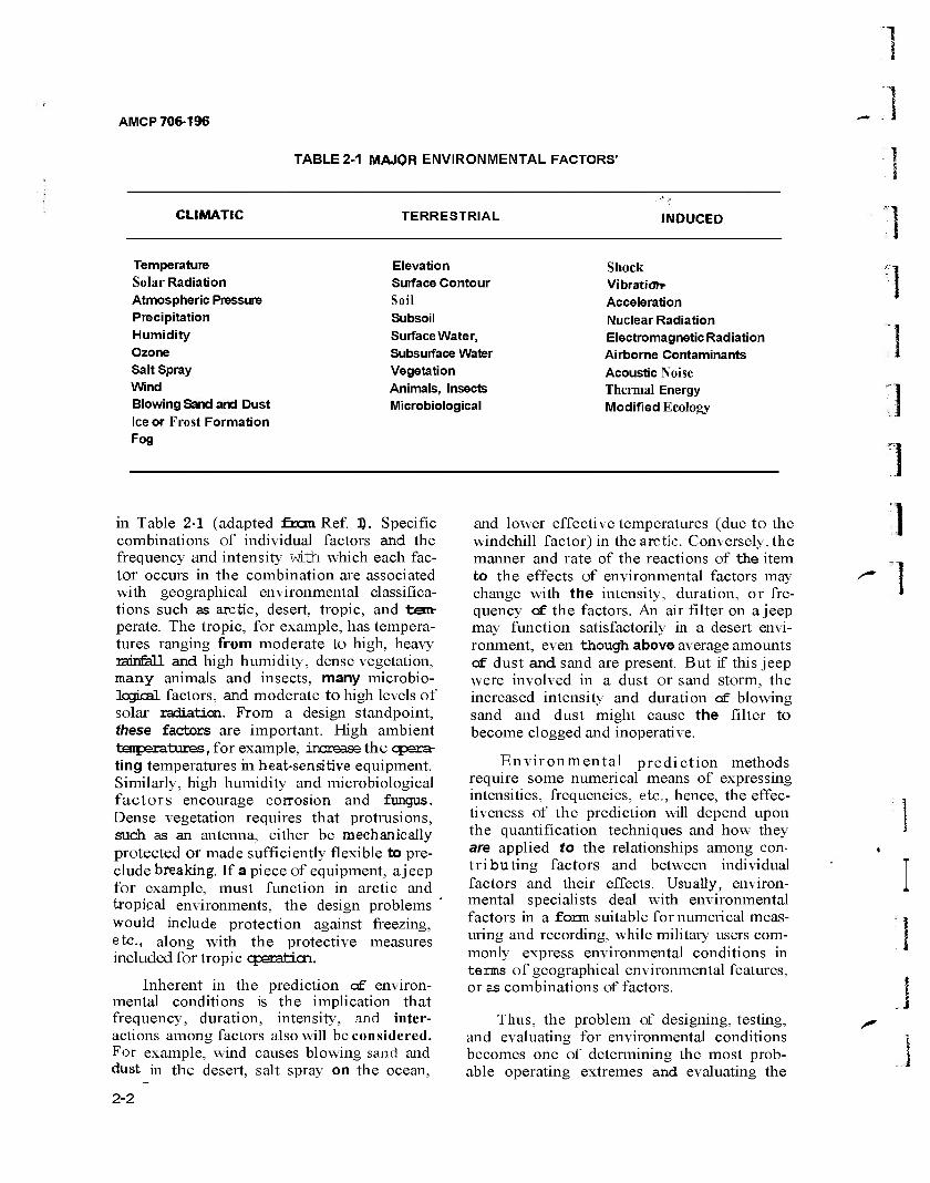
AMCP 706-196

TABLE 2-1 MAJOR ENVIRONMENTAL FACTORS'

CLIMATIC TERRESTRIAL INDUCED

Temperature Solar Radiation Atmospheric Pressure Precipitation Humidity Ozone Salt Spray Wind Blowing Sand and Dust Ice or Frost Formation Fog

Elevation Surface Contour Soil Subsoil Surface Water, Subsurface Water Vegetation Animals, Insects Microbiological

Shock Vibratidrr Acceleration Nuclear Radiation Electromagnetic Radiation Airborne Contaminants Acoustic Noise Thermal Energy Modified Ecology

in Table 2-1 (adapted fron Ref. 1). Specific combinations of individual factors and the frequency and intensity wLtti which each factor occurs in the combination are associated with geographical environmental classifications such as arctic, desert, tropic, and tarr perate. The tropic, for example, has temperatures ranging from moderate to high, heavy rainfall and high humidity, dense vegetation, many animals and insects, many microbiological factors, and moderate to high levels of solar radiation. From a design standpoint, these factors are important. High ambient tenperatures, for example, increase the operating temperatures in heat-sensitive equipment. Similarly, high humidity and microbiological factors encourage corrosion and fungus. Dense vegetation requires that protrusions, such as an antenna, either be mechanically protected or made sufficiently flexible to preclude breaking. If a piece of equipment, a jeep for example, must function in arctic and tropical environments, the design problems would include protection against freezing, etc., along with the protective measures included for tropic cparatLcn.

Inherent in the prediction of environmental conditions is the implication that frequency, duration, intensity, and interactions among factors also will be considered. For example, wind causes blowing sand and dust in the desert, salt spray on the ocean,

and lower effective temperatures (due to the windchill factor) in the arctic. Conversely, the manner and rate of the reactions of the item to the effects of environmental factors may change with the intensity, duration, or frequency of the factors. An air filter on a jeep may function satisfactorily in a desert environment, even though above average amounts of dust and sand are present. But if this jeep were involved in a dust or sand storm, the increased intensity and duration of blowing sand and dust might cause the filter to become clogged and inoperative.

Environmental prediction methods require some numerical means of expressing intensities, frequencies, etc., hence, the effectiveness of the prediction will depend upon the quantification techniques and how they are applied to the relationships among contributing factors and between individual factors and their effects. Usually, environmental specialists deal with environmental factors in a form suitable for numerical measuring and recording, while military users commonly express environmental conditions in terms of geographical environmental features, or as combinations of factors.

Thus, the problem of designing, testing, and evaluating for environmental conditions becomes one of determining the most probable operating extremes and evaluating the

i

2-2

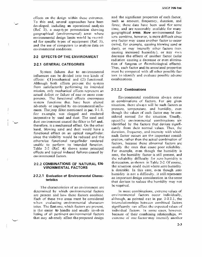
AMCP 706-1 ab

effects on the design within these extremes. To this end, several approaches have been developed, including an operational analysis (Ref. 2), a map-type presentation showing geographical (environmental) areas where environmental design limits would be exceeded for specific types of equipment (Ref. 3), and the use of computers to analyze data on environmental conditions.

2-2 EFFECTS OF THE ENVIRONMENT

2-2.1 GENERAL CATEGORIES

System failures due to environmental influences can be divided into two kinds of effects: (1)mechanical and (2) functional. Although both effects prevent the system from satisfactorily performing its intended mission, only mechanical effects represent an actual defect or failure of one or more components. The functional effects encompass system functions that have been altered adversely or impeded by environmental influences. The jeep filter mentioned in par. 2-1.2, for example, was clogged and rendered inoperative by sand and dust. The sand and dust environment caused the filter to fail and. therefore, is a mechanical effect. On the other hand, blowing sand and dust would have a functional effect on an optical rangefinder: since the visibility would be reduced and the otherwise functional rangefinder rendered unable to perform its intended function. Table 2-2 (Ref. 4) shows some principal effects and typical induced failures caused by environmental factors.

2-2.2 COMBINATIONS OF NATURAL EN- VIRONMENTAL FACTORS

2-2.2.1 Evaluation of Environmental Charac- teristics

The characteristics of an environment are determined by which environmental factors are present and how these factors combine. Each of these two areas must be considered when evaluating environmental characteristics. The first one, which factors are present, is the easier to handle and usually involves listing of all pertinent environmental factors that may adversely affect the proposed design

and the significant properties of each factor, such as amount, frequency, duration, and force; these data have been used €or some time, and are reasonably available for many geographical areas. How environmental factors combine, however, is more difficult since one factor may cause another factor to occur (wind, for example, causing blowing sand or dust), or may intensify other factors (rain causing increased humidity), or may evtn decrease the effects of another factor (solar radiation causing a decrease or even elimination of fungous or microbiological effects). Thus, each factor and its associated properties must be compared with all other possible factors to identify and evaluate possible adverse combinations.

2-2.2.2 Combinations

Environmental conditions always occur as combinations of factors. For any given situation, there always will be such factors as pressure, temperature, and humidity, even though the values of each factor may be considered normal for the situation. Usually, specific environmental combinations are identified by the factors that deviate significantly from their normal values. Thus, the duration, frequency, and intensity with which each factor occurs are the important consideration, rather than the actual combination of factors, because these abnormal factors are usually the ones that cause poor reliability. For example, even though the humidity is zero, the humidity factor is still present, and the reliability difficulty for zero humidity is desiccation, as shown in Table 2-2. Of course, the situation could exist where zero humidity is desirable. In this case, even though zero humidity is not a difficulty, it still represents an important design consideration in the sense that devices to reduce the humidity may not be required.

In most combinations, extreme values of environmental factors occur individually, although, as pointed out in par. 2-2.2.1, the interrelationships between combined factors significantly can affect the expected values of individual factors. In some cases, however, because of their combining relationships, an extreme of one factor may intensify another

2-3

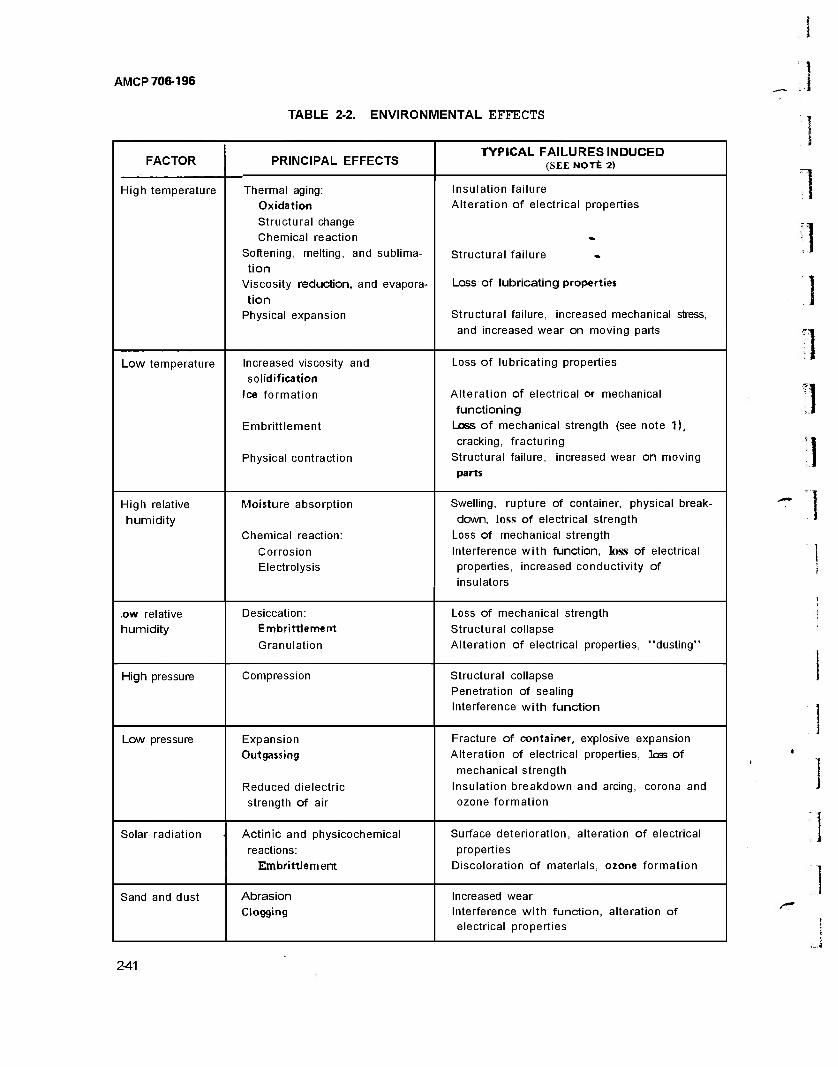
AMCP 706-196

TABLE 2-2. ENVIRONMENTAL EFFECTS

FACTOR PRINCIPAL EFFECTS TYPICAL FAILURES INDUCED

(SEE NOTfe 2)

High temperature Thermal aging:

Oxidation

Structural change

Chemical reaction

Softening, melting, and sublima-

tion Viscosity reduction, and evapora-

tion Physical expansion

Insulation failure

Alteration of electrical properties

Structural failure -

Loss of lubricating properties

Structural failure, increased mechanical stress,

and increased wear on moving parts

Low temperature Increased viscosity and

solidification

Ice formation

Embrittlement

Physical contraction

Loss of lubricating properties

Alteration of electrical or mechanical

functioning

Loss of mechanical strength (see note 1),

cracking, fracturing

Structural failure, increased wear on moving

parts

High relative

humidity

Moisture absorption

Chemical reaction:

Corrosion Electrolysis

Swelling, rupture of container, physical break-

down, loss of electrical strength

Loss of mechanical strength

Interference with function, loss of electrical

properties, increased conductivity of

insulators

,ow relative humidity

Desiccation: Embrittlement

Granulation


Structural collapse

Alteration of electrical properties, "dusting"

High pressure Compression Structural collapse

Penetration of sealing

Interference with function

Low pressure Expansion

Out gassing

Reduced dielectric

strength of air

Fracture of container, explosive expansion

Alteration of electrical properties, 1cm of

mechanical strength

Insulation breakdown and arcing, corona and ozone formation

Solar radiation ■ Actinic and physicochemical

reactions: Embrittle merit

Surface deterioration, alteration of electrical

properties

Discoloration of materials, ozone formation

Sand and dust Abrasion Clogging

Increased wear Interference with function, alteration of electrical properties

3

241

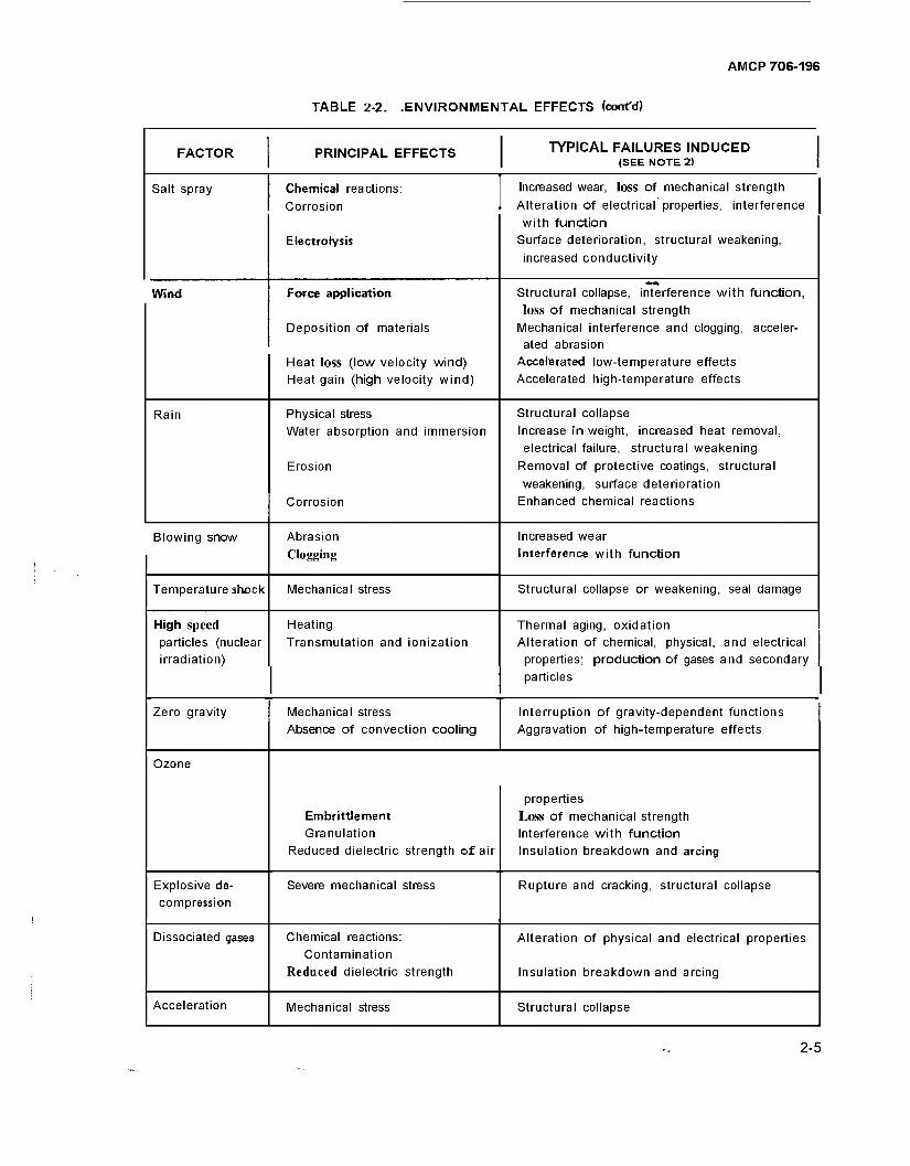
AMCP 706-196

TABLE 2-2. .ENVIRONMENTAL EFFECTS (cont'd»

FACTOR PRINCIPAL EFFECTS I TYPICAL FAILURES INDUCED I | (SEE NOTE 2) |

Salt spray Chemical reactions:

Corrosion

Electrolysis

Increased wear, loss of mechanical strength

Alteration of electrical properties, interference

with function

Surface deterioration, structural weakening,

increased conductivity

Wind Force application

Deposition of materials

Heat loss (low velocity wind) Heat gain (high velocity wind)

Structural collapse, interference with function,

loss of mechanical strength

Mechanical interference and clogging, accelerated abrasion

Accelerated low-temperature effects

Accelerated high-temperature effects

Rain Physical stress

Water absorption and immersion

Erosion

Corrosion

Structural collapse

Increase in weight, increased heat removal,

electrical failure, structural weakening

Removal of protective coatings, structural

weakening, surface deterioration

Enhanced chemical reactions

Blowing snow Abrasion

Clogging

Increased wear


Temperature ahcck Mechanical stress Structural collapse or weakening, seal damage

High speed

particles (nuclear irradiation)

Heating

Transmutation and ionization

Thermal aging, oxidation Alteration of chemical, physical, and electrical

properties; production of gases and secondary

particles

Zero gravity Mechanical stress

Absence of convection cooling

Interruption of gravity-dependent functions

Aggravation of high-temperature effects

Ozone

Embrittlement

Granulation

Reduced dielectric strength of air

properties



Insulation breakdown and arcing

Explosive de-

compression

Severe mechanical stress Rupture and cracking, structural collapse

Dissociated gases Chemical reactions:

Contamination

Reduced dielectric strength

Alteration of physical and electrical properties

Insulation breakdown and arcing

Acceleration Mechanical stress Structural collapse

2-5

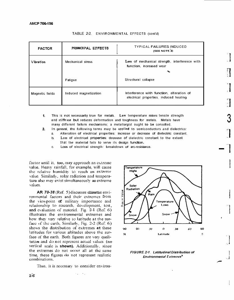
AMCP 706-196

TABLE 2-2. ENVIRONMENTAL EFFECTS (cont'd)

FACTOR PRINCIPAL EFFECTS TYPICAL FAILURES INDUCED (SEE NOTE 1)

Vibration Mechanical stress

Fatigue

Loss of mechanical strength, interference with function, increased wear

Structural collapse

Magnetic fields Induced magnetization Interference with function, alteration of electrical properties, induced heating

This is not necessarily true for metals. Low temperature raises tensile strength

and stiffness but reduces deformation and toughness for metals. Metals have

many different failure mechanisms; a metallurgist ought to be consulted.

In general, the following terms may be applied to semiconductors and dielectrics:

a. Alteration of electrical properties: increase or decrease of dielectric constant.

b. Loss of electrical properties: decrease of dielectric constant to the extent

that the material fails to serve its design function. c. Loss of electrical strength: breakdown of arc-resistance.

3

-1 factor until it, too, may approach an extreme value. Heavy rainfall, for example, will cause the relative humidity to reach an extreme value. Similarly, solar radiation and temperature also may exist simultaneously as extreme values.

AR 70-38 (Ref. 5) discusses climatic environmental factors and their extremes from the viewpoint of military importance and relationship to research, development, test, and evaluation of materiel. Fig. 2-1 (Ref. 6) illustrates the environmental extremes and how they vary relative to latitude at the surface of the earth, Similarly, Fig. 2-2 (Ref. 6) shows the distribution of extremes at these latitudes for various altitudes above the surface of the earth. Both figures are very qualitative and do not represent actual values (no vertical scale is shown). Additionally, since the extremes do not occur all at the same time, these figures <lo not represent realistic combinations.

Thus, it is necessary to consider environ-

Temperature Highs

7

90

N

60 30 O 30

Latitude

60 90

FIGURE 2-1. Latitudinal Distribution of Environmental Extremes'"

1

■A

2-6

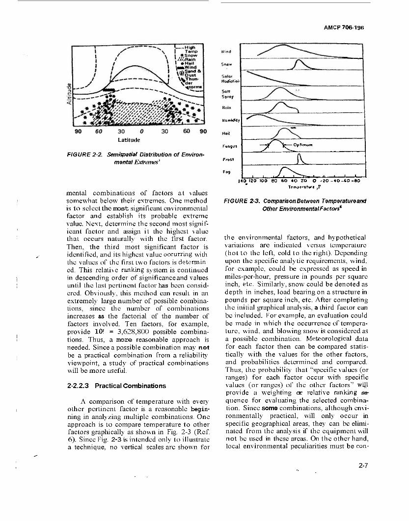
A MCP 706-196

Latitude

FIGURE 2-2. Semispatial Distribution of Environ- mental Extremes'

mental combinations of factors at values somewhat below their extremes. One method is to select the most significant environmental factor and establish its probable extreme value. Next, determine the second most significant factor and assign it the highest value that occurs naturally with the first factor. Then, the third most significant factor is identified, and its highest value occurring with the values of the first two factors is determined. This relative ranking system is continued in descending order of significance and values until the last pertinent factor has been considered. Obviously, this method can result in an extremely large number of possible combinations, since the number of combinations increases as the factorial of the number of factors involved. Ten factors, for example, provide 10! = 3,628,800 possible combinations. Thus, a more reasonable approach is needed. Since a possible combination may not be a practical combination from a reliability viewpoint, a study of practical combinations will be more useful.

2-2.2.3 Practical Combinations

A comparison of temperature with every other pertinent factor is a reasonable beginning in analyzing multiple combinations. One approach is to compare temperature to other factors graphically as shown in Fig. 2-3 (Ref. 6). Since Fig. 2-3 is intended only to illustrate a technique, no vertical scales are shown for

Mumldity

Fungus

Frost

Fog

•y~x^ Optimum

JL |40 120 »00 eO 60 40 20 O -2O-40-S0-80

TtmpK-atiK« ,F

FIGURE 2-3. Comparison Between Temperature and Other Environmental Factors6

the environmental factors, and hypothetical variations are indicated versus temperature (hot to the left, cold to the right). Depending upon the specific analytic requirements, wind, for example, could be expressed as speed in miles-per-hour, pressure in pounds per square inch, etc. Similarly, snow could be denoted as depth in inches, load bearing on a structure in pounds per square inch, etc. After completing the initial graphical analysis, a third factor can be included. For example, an evaluation could be made in which the occurrence of temperature, wind, and blowing snow is considered as a possible combination. Meteorological data for each factor then can be compared statistically with the values for the other factors, and probabilities determined and compared. Thus, the probability that "specific values (or ranges) for each factor occur with specific values (or ranges) of the other factors" will provide a weighting or relative ranking sequence for evaluating the selected combination. Since some combinations, although envi- ronmentally practical, will only occur in specific geographical areas, they can be eliminated from the analysis if the equipment will not be used in these areas. On the other hand, local environmental peculiarities must be con-

2-7

AMCP 706-196

sidered carefully in any study, since they may create effects that o ;herwise would go unde- tected in a generalised analysis over a large area. Furthermore, nany optimistic predictions of the future nre wrong; "if the worst can happen, it will happen."

In addition to the graphical approach, environmental factors may be combined in pairs and analyzed by a chart similar to Table 2-3 (Ref. 7). The techniques involved in developing a chart are similar to those for the graphical method, and the same general comments apply to both approaches.

2-2-3 COMBINATIONS OF INDUCED ENVIRONMENTAL FACTORS

All environmental conditions are influenced to some extent by the presence of man or man's products. The basic act of breathing, for example, consumes oxygen and releases carbon dioxide and water vapor into the atmosphere. While the breathing of one man in the middle of a forest will not cause a noticeable change in the concentrations of oxygen, water vapor, or carbon dioxide, the change is extremely important in the closed atmosphere of a spacecraft life-support system. Similarly, the motion of a hydraulic piston causes shock and vibration, and the piston operating pressure and friction create heat. If the piston ir take stroke allows moisture to enter the cylinder, the moisture may cause corrosion which, in turn, could lead to increased friction, ; greater wear, and additional heat. Any contaminants, such as sand or dust, that enter the cylinder with the moisture will also contribute to increased friction, wear, and leat. Even the color of paint used on equipn.ent can affect reliability, since optically light colors such as white or silver also reflect significant amounts of infrared, while optically i lark colors such as black or olive-drab will cause higher internal temperatures by absorbing infrared. These examples illustrate that induced environmental factors, either singly or in combination, represent the major environmental problems from a reliability viewpoint.

2-2.4 ENVIRONMENTAL ANALYSIS

After establishing the desired equipment

parameters and roughing out the initial design, the designer ought to analyze the probable operating environment. The results can then be applied to system components to determine the environments experienced by individual components and how these individual environments will affect component operation and reliability. Thus, individual part specifications can be selected to compensate for environmental influences, rather than having to add environmental compensating methods after the design has progressed to more advanced stages. The environmental analysis must consider all phases of the mission profile, i.e., the equipment stockpile- to-target sequence. Some of the distinct phases that must be evaluated are transportation, handling, storage, standby-idle time, standby-active time, use or operational tiie, and maintenance. Each phase creates its own peculiar influences on equipment reliability. The circulation of air during operation, for example, may prevent the accumulation of moisture or dust, while the same item in storage may not have this circulation and may corrode or grow fungus. Table 2-4 (adapted from Ref. 6) shows some effects of natural and induced environments during the various phases of the lifetime of an item. Table 2-5 (adapted from Ref, 6)provides reliability considerations for pairs of environmental factors. Ref. 7 gives more information on combinations of environments.

2-3 DESIGNING FOR THE ENVIRON- MENT

Equipment failures have three convenient classifications:

(1) Poor design or incorrect choice of materials or components

(2) Inadequate . quality control which permits deviations from design specifications

(3) Deterioration caused by environmental effects or influences.

The perceptive reader, at this point, wDl have observed that the first and third classes are related. Specifically, the careful selection of design and materials can extend item reliability by reducing or eliminating adverse environmental effects. Needless to say, this is not a profound thought, but merely one that is

1

I n

2-8

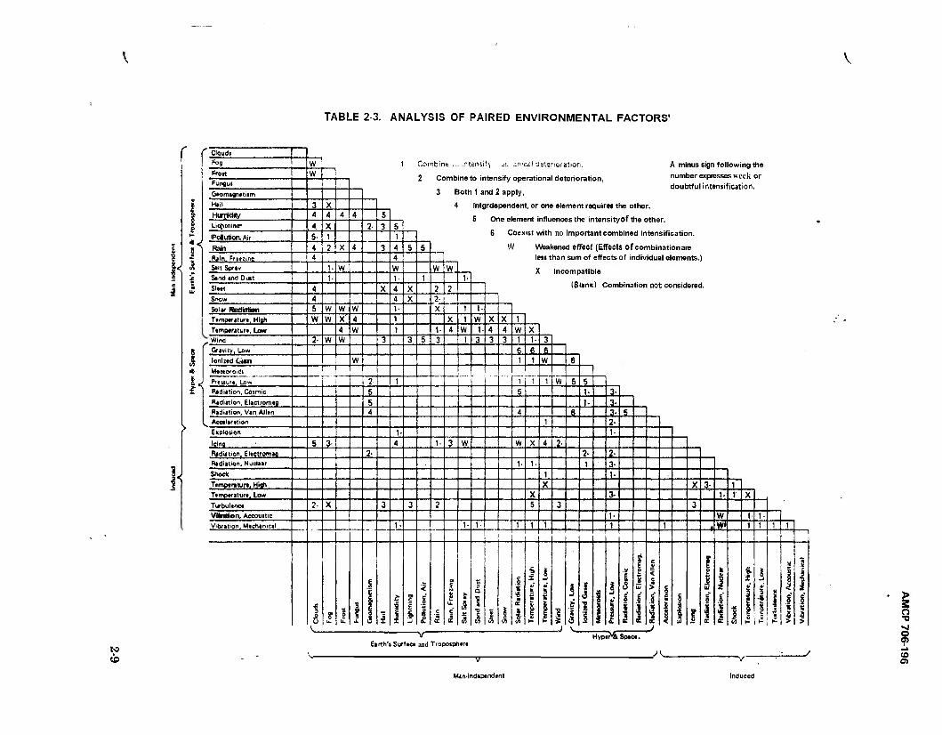
TABLE 2-3. ANALYSIS OF PAIRED ENVIRONMENTAL FACTORS'

bo

r Cloudi

Fog w 1 Combine ... .mensi^ .c. inicäl deterioration, A minus sign following the Fro« w o f-»»ki..i, i.k,.,a .;...u .: number expresses week or Fungut

Geomegnetiim 3 Both 1 and 2 apply,

Hail 3 X 4 Intgrdependent, or one element reauirei the other. % Humidity 4 4 4 4 5

0 Ltqt\tninp- 4 X 2- 3 5 >- Pollution. Air 6' 1 1 b wexisi with no important combined intensification.

1 Ran 4 2 X 4 3 4 6 5 W Weakened effect (Effects of combinational«

Rain, Fr«e:ino 4 4 Im than sum of effects of individual elements.) «a Sad Sprjy 1- W W W W

i Sind and Duct 1- 1- 1- 1- SlMl 4 X 4 X 2 2 lölank) Combination not considered.

Snow 4 4 X 2- Sola/ Radiaton 5 W w W 1- X 1 1- Temperature, High W W X 4 1 X 1 w X X 1 Temperature, Low 4 W 1 1- 4 W 1- 4 4 W X

^Wind 2- w w 3 3 5 3 1 3 3 3 1 1- 3

I Gravity, Low 6 6 6 Ionized Li.ui w i 1 w 6

* Meteoroids

i< Prewure, Low 2- 1 i- i 1 w 5 5 Radiation, Coimic ? 5 1- 3- Radiation, Electromeg 5 1- 3- Radiation, Van Allen 4 4 9 3- 5

^ Acceleration 1 2- Exploiion 1- 1- tcinj S 3- 4 1- 3 W W X 4 2- Radiation, Electromeg 2- 2- ?• Radiation, Nuclear 1- 1- 1 3- Shock 1 1- Temperature, High X X 3- 1 Temperatur«, Low X 3- 1- 1 X Turbulence 2- X 3 3 2 5 3 3 VUnMion, Accouitic 1- W 1 1- Vibration, Mechanical 1- 1- 1- 1 1 1 1 1 w* 1 1 i 1

"' l

1 0 Ü

? u.

1 3

f u.

i

I i ■i E 3 I

? C

1

<

I c '5 a

a c

| c 3

a:

>• n

c

3 a

I -o 1 s

c o % m

<r 5

s

|

I I «* s s

1

1

J J 1 1

| J V 8

1 "S

t S |

I

c * < s > i 1

1 m i 1

i 5 I

1 Hi

J .« -» a

1

i ,

2 »V*

3

1 w r*

I -> •V

5 -S i c

3

i ?

8 '6 >

1 1 i 1' s >

. -

V Hyper* So.«. Eerlh'l Surface and Tropoiphere

v _,

Ind

J

M ian-i

V

id«p< inda nt

i

jced

>

•a (O en

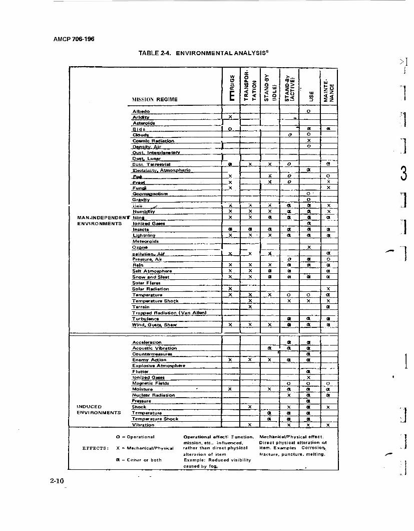
AMCP 706-196

TABLE 2-4. ENVIRONMENTAL ANALYSIS6

MISSION REGIME

W O a re

E

e O

3 I < r- CC < 1- r-

> m a — < J

vt s

o>

r-< UJ —

Ul (4 3

UJ |_ Ul

II Albedo O

Aridity X ^ Asteroids

0 Bids 9 a

Clouds a O

Cosmic Radiation . X

Re,nsity. Air J o

Oust. Interplanetary

Dust, Lunar Dust, Terrestrial a X X o a

Tiia^+i-iîtv. Atmospheric a F<m X X o O

fro«rt X X o X Funsü X X

Geomag nettem o Gravity o nail sf X "X "X a a X

Humidity X X X a a X MAN.INDEPENDENTT Icing X X a a a a ENVIRONMENTS Ionized Gases a

Insects a a a a a a Lightning X X - X a a a Meteoroids Ozone

X X

X

p^n»ti-9-f>.. A+r * a Pressure, Air o a o Rain X X X a a a Salt Atmosphere X X a a a Snow and Sleet X X a a a a Solar Flares Solar Radiation X X

Temperature X X X o o a Temperature Shock X X X X

Terrain X a Trapped Radiation (Van Allen)

Turbulence a a a Wind, Gusts, Shear X X X a a a

Acceleration a a Acoustic Vibration a a a Countermeasures i a Enemy Action X X X a a Explosive Atmosphere Flutter a Ionized Gases X Magnetic Fields o o o Moisture X X a a a Nuclear Radiation X a a Pressure a

INDUCED Shock X X a X ENVIRONMENTS Temperature a a a

Temperature Shock a a a Vibration X X X X

O = Operational Operational effect: Function. mission, etc.. influenced,

EFFECTS: X = Mechanical/Physical rather than direct physical

alterarion of item a = Enher or both Example: Reduced visibility

caused by fog^

vlechanical/Physical effect: Direct physical alteration of tern. Examples Corrosion.,

racture. puncture, melting.

>I

3

1

2-10

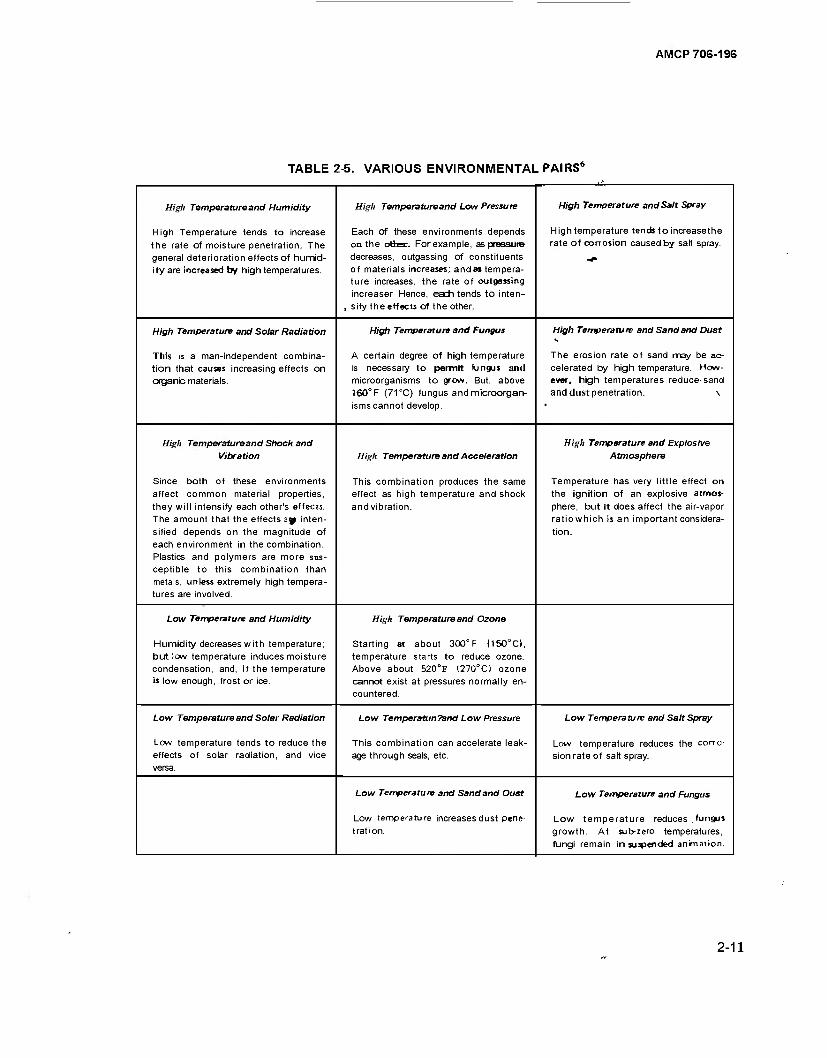
AMCP 706-196

TABLE 2-5. VARIOUS ENVIRONMENTAL PAIRS6

High Temperature and Humidity

High Temperature tends to increase the rate of moisture penetration. The general deterioration effects of humidity are increased by high temperatures.

High Temperatureand Low Pressure

Each of these environments depends on the other. For example, as pressure decreases, outgassing of constituents of materials increases; andas temperature increases, the rate of outgassing increaser Hence, each tends to inten-

, sify the effects of the other.

High temperature and Salt Spray

High temperature tends to increasethe rate of corrosion caused by salt spray.

High Temperature and Solar Radiation

This is a man-independent combination that causes increasing effects on organic materials.

High Temperatun and Fungus

A certain degree of high temperature is necessary to permit fungus and microorganisms to grow. But. above 160°F (71°C) fungus and microorganisms cannot develop.

High Temperature and Sandand Dust

The erosion rate of sand may be accelerated by high temperature. How- ever, high temperatures reduce-sand and dust penetration. \

High Temperatureand Shock and Vibration

Since both of these environments affect common material properties, they will intensify each other's effects. The amount that the effects ay inten- sified depends on the magnitude of each environment in the combination. Plastics and polymers are more susceptible to this combination than metals, unless extremely high temperatures are involved.

High Temperatureand Acceleration

This combination produces the same effect as high temperature and shock andvibration.

High Temperature and Explosive Atmosphere

Temperature has very little effect on the ignition of an explosive atmosphere, but it does affect the air-vapor ratiowhich is an important consideration.

Low Temperature and Humidity

Humidity decreases with temperature; but low temperature induces moisture condensation, and, if the temperature is low enough, frost or ice.

High Temperatureand Ozone

Starting at about 300°F (150°C), temperature starts to reduce ozone. Above about 520°F (270°C) ozone cannot exist at pressures normally encountered.

Low Temperatureand Solar Radiation

Low temperature tends to reduce the effects of solar radiation, and vice versa.

Low TemperatunTand Low Pressure

This combination can accelerate leakage through seals, etc.

Low Temperature and Salt Spray

Low temperature reduces the corrosion rate of salt spray.

Low Temperature and Sandand Oust

Low temperature increases dust penetration.

Low Temperature and Fungus

Low temperature reduces fungus growth. At sub-zero temperatures, fungi remain in suspended animation.

2-11

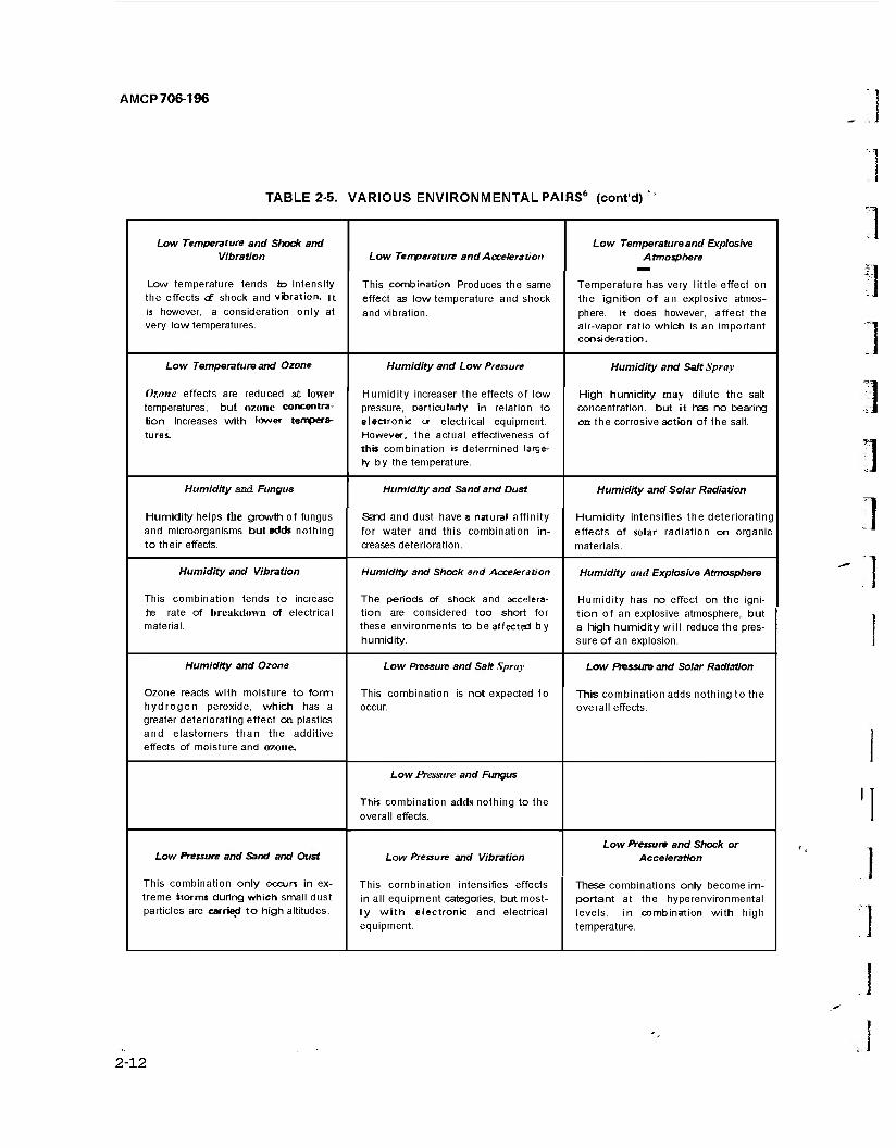
AMCP 706-196

TABLE 2-5. VARIOUS ENVIRONMENTAL PAIRS6 (cont'd)

Low Temperature and Shock and Vibration

Low temperature tends to intensify the effects <£ shock and vibration, it is however, a consideration only at very low temperatures.

Low Temperature and Acceleration

This combination Produces the same effect as low temperature and shock and vibration.

Low Temperature and Explosive Atmosphere

Temperature has very little effect on the ignition of an explosive atmosphere. It does however, affect the air-vapor ratio which is an important consideration.

Low Temperature and Ozone

Ozone effects are reduced at lower temperatures, but ozone concentration increases with lower temperatures.

Humidity and Low Pressure

Humidity increaser the effects of low pressure, particularly in relation to electronic or electrical equipment. However, the actual effectiveness of this combination is determined largely by the temperature.

Humidity and Salt Spray

High humidity may dilute the salt concentration, but it has no bearing on the corrosive action of the salt.

Humidity and Fungus

Humidity helps the growth of fungus and microorganisms but adds nothing to their effects.

Humidity and Sand and Dust

Sand and dust have a natural affinity for water and this combination increases deterioration.

Humidity and Solar Radiation

Humidity intensifies the deteriorating

effects of solar radiation on organic materials.

Humidity and Vibration

This combination tends to increase tie rate of breakdown of electrical material.

Humidity and Shock and Acceleration

The periods of shock and acceleration are considered too short for these environments to be affected by humidity.

Humidity and Explosive Atmosphere

Humidity has no effect on the ignition of an explosive atmosphere, but a high humidity will reduce the pressure of an explosion.

Humidity and Ozone

Ozone reacts with moisture to form hydrogen peroxide, which has a greater deteriorating effect on plastics and elastomers than the additive effects of moisture and ozone.

Low Pressure and Salt Spray

This combination is not expected to occur.

Low Pressure and Solar Radiation

This combination adds nothing to the overall effects.

Low Pressure and Fungus

This combination adds nothing to the overall effects.

Low Pressure and Sand and Oust

This combination only occur» in extreme storms during which small dust particles are carried to high altitudes.

Low Pressure and Vibration

This combination intensifies effects in all equipment categories, but mostly with electronic and electrical equipment.

Low Pressure and Shock or Acceleration

These combinations only become important at the hyperenvironmental levels, in combination with high temperature.

2-12

AMCP 706-196

TABLE 2-5. VARIOUS ENVIRONMENTALPAIRS6 (cont'd)

Low Pressure and Explosiv» Atmosphere

At low pressures an electrical dk- charge is easier to develop, but the explosive atmosphere is harder to ignite.

Sal? Spray and Fungus

This is considered an incompatible combination.

Salt^Spray and Sand and Dust

Thk wMI have the same combined effect as humidity end sand and dust.

Salt Spray and Vibration

This will have the same combined effect as humidity and vibration.

Salt Spray and Shock or Acceleration

These combinations will produce no added effects.

Salt Spray and Explosive Atmosphere

This is considered an incompatible combination.

Sa/t Spray and Ozone

These environments have the same combined effect as humidity and ozone.

Solar Radiation and Fungus

Because of the resuming heat from solar radiation, this combination probably produces the same combined effect as high temperature and fungus. Further, the ultraviolet inun- filtered radiation is an effective fungi- cide.

Solar Radiation and Sand and Dust

It is suspected that this combination will produce high temperatures.

Solar Radiation and Ozone

This combination increases the rate of oxidation of materials.

fungus and Ozone

Fungus is destroyed by ozone.

Solar Radiation and Shock or Acceleration

These combinations produce no additional effects.

Solar Radiation and Vibration

Under vibration conditions, solar radiation deteriorates plastics, elastomers, oils, etc., at a higher rate.

Sand and Dust and Vibration

Vibration might possibly increase the wearing effects of sand and dust.

Shock and Vibration

This combination produces no added effect.

Vibration and Acceleration

This combination produces increased effects when encountered with high temperatures and low pressures in the hyperenvironmental ranges.

Solar Radiation and Explosive A tmosphere

This combination produces no added effects.

2-13

AMCP706-196

sometimes forgotten or perhaps relegated to mental footnotes. The environment is neither forgiving nor understanding; it methodically surrounds and attacks every component of a system, and when a weak point easts, the equipment reliability suffers. Design and reliability engineers, therefore, must understand the environment and its potential effects, and then must select designs or materials that counteract these effects or must provide methods to alter or control the environment within acceptable limits. Selecting designs or materials that withstand the environment has the advantage of not requiring extra components that also require environmental protection and add weight and costs.

In addition to the obvious environments of temperature, humidity, shock, and vibration, the design engineer will create environments by his choice of designs and materials. A gasket car seal, for example, under elevated temperatures or reduced pressures may release corrosive cr degrading volatiles into the system. Teflon may release fluorine, and Poly- vinylchloride (PVC) may release chlorine. Certain solid rocket fuels are degraded into a jelly-like nass when exposed to aldehydes or ammonia, either of which can come from a phenolic nozzle cone. These examples illustrate that internal environments designed into the system can seriously affect reliability.

Many aids are available to design and reliability engineers in selecting materials and components, e.g., the text, Deterioration of Materials, Causes and Preventive Techniques, by Glenn A. Greathouse and Carl J. Wessel (Ref. 8). In addition, military specifications, standards, and handbooks provide both general and specific guidance on this subject. Appendix B lists data banks that consolidate and evaluate materials and components from the reliability viewpoint.

2-3.1 TEMPERATURE PROTECTION

Heat arid cold are powerful agents of chemical and physical deterioration for two very simple, basic reasons:

(l)The physical properties of almost all known materials are modified greatly by changes in temperature.

(2) The rate of almost all chemical reactions is influenced markedly by the temperature of the reactants. A familiar rule-of-thumb for chemical reactions is that the rate of many reactions doubles for every -rise in temperature of 10 degC (Ref. 8);this is equivalent to an activation energy of about 0.6 eV.

Basically, heat is transferred by three methods: (1) radiation, (2^ conduction, and (3) convection. One, or a "combination of

these three methods, therefore, is used to protect against temperature degradation. High temperature degradation can be minimized by passive or active techniques. Passive techniques use natural heat sinks to remove heat, while active techniques use devices such as heat pumps or refrigeration units to create heat sinks. Such design measures as compart- mentation, insulation of compartment walls, and intercompartment and intrawall air flow can be applied independently or in combination. Every system component should be studied from two viewpoints:

(1) Is a substitute available that will generate less heat?

(2) Can the component be located and positioned so that its heat has minimum effect on other components?

For a steady temperature, heat must be removed at the same rate at which it is generated- Thermal systems such as conduction cooling, forced convection, blowers, direct or indirect liquid cooling, direct vaporization or evaporation cooling, and radiation cooling must be capable of handling both natural and induced heat sources. Fig. 2-4 compares the effectiveness of several such methods.

Passive sinks require some means of progressive heat transfer from intermediate sinks to ultimate sinks until the desired heat extrac- tion has been achieved. Thus, when heat sources have been identified, and heat removal elements selected, they must be integrated into an overall heat removal system, so that heat is not merely redistributed within the system. Efficiently integrated heat removal techniques can significantly improve item reliability.

Besides the out-gassing of corrosive volatiles when subjected to heat, almost all known

2-14,

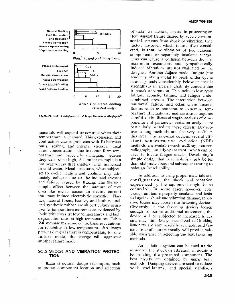
AMCP 706-19S

Natural Cooling\

Free Convection V and Radiation'

Forced Convection Direct Liquid Cooling Vaporization Cooling

0 5 10

W/in.2 {based on 40 deg 0 rise)

Plastic Embedment

Free Air

Metallic Conduction

Forced Convection

Direct Liquid Cooling

Vaporization Cooling

« OS 1 5

t 5 Max

1 1 1 1

10 15 20

W/:n - (for internal cooling of sealed units)

FIGURE 2-4. Comparison of Heat Removal Methods6

materials will expand or contract when their temperature is changed, This expansion and contraction causes problems with fit between parts, sealing, and internal stresses. Local stress concentrations due to nonuniform temperature are especially damaging, because they can be so high, A familiar example is a hot water-glass that shatters when immersed in cold water, Metal structures, when subjected to cyclic heating and cooling, may ulti- mately collapse due to the induced stresses and fatigue caused by flexing. The thermo- couple effect between the juncture of two dissimilar metals causes an electric current that may induce electrolytic corrosion. Plas- tics, natural fibers, leather, and both natural and synthetic rubber are all particularly sensitive to temperature extremes as evidenced by their brittleness at low temperatures and high degradation rates at high temperatures. Table 2-6 summarizes some of the basic precautions for reliability at low temperatures. An always present danger is that in compensating for one failure mode, the change will aggravate another failure mode.

2-3.2 SHOCK AND VIBRATION PROTEC- TION

Basic structural design techniques, such as proper component location and selection

of suitable materials, can aid in protecting an item against failure caused by severe environmental stresses from shock or vibration, One factor, however, which is not often considered, is that the vibration of two adjacent components or separately insulated subsystems can cause a collision between them if maximum excursions and sympathetically induced vibrations are not evaluated by the designer. Another failure mode, fatigue (the tendency Sor a metal to break under cyclic stressing loads considerably below its tensile strength) is an area of reliability concern due to shock or vibmtion. This includes low cycle fatigue, acoustic fatigue, and fatigue under combined stresses. The interaction between multiaxial fatigue and other environmental factors such as temperature extremes, temperature fluctuations, and corrosion requires careful study. Stress-strength analysis of components and parameter variation analysis are particularly suited to these effects. Destruc- tive testing methods are also very useful in this area. For one-shot devices, several efficient nondestructive evaluation (NDE) methods are available—such as X ray, neutron radiography, and dye-penetrant—which can be used to locate fatigue cracks. Developing'a simple design that is reliable is much better than elaborate fixes and subsequent testing to redesign for reliability.

In addition to using proper materials and configuration, the shock and vibration experienced by the equipment ought to be controlled. In some cases, however, even though an item is properly insulated and isolated against shock and vibmtion damage, repetitive forces may loosen the fastening devices. Obviously, if the fastening devices loosen enough to permit additional movement, the device will be subjected to increased forces and may fail. Many specialized self-locking fasteners are commercially available, and fas-< tener manufacturers usually will provide valuable assistance in selecting the best fastening methods.

An isolation system can be used at the source of the shock or vibration, in addition to isolating the protected component- The best results am obtained by using both methods. Damping devices are used to reduce peak oscillations, and special stabilizers

2-15

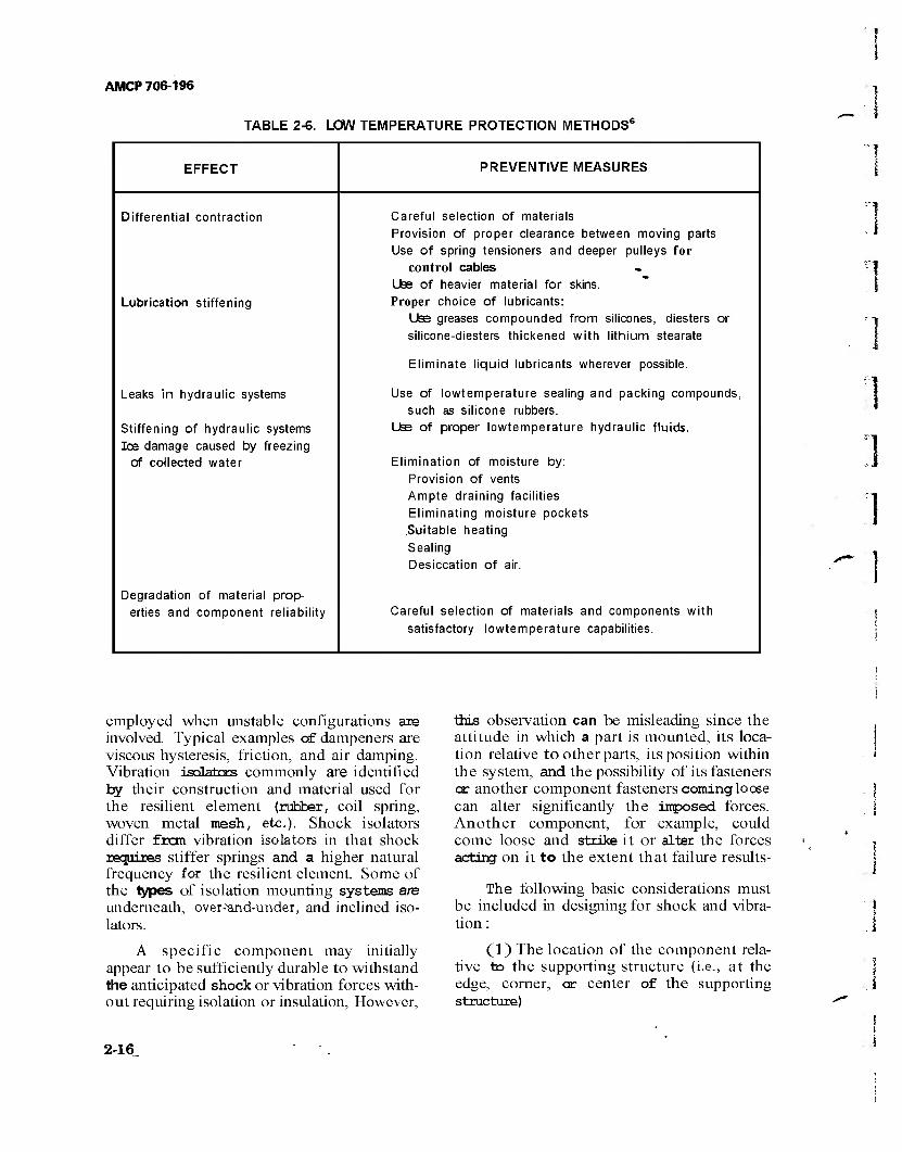
AMCP 706-196

TABLE 2-6. LOW TEMPERATURE PROTECTION METHODS6

EFFECT PREVENTIVE MEASURES

Differential contraction

Lubrication stiffening

Leaks in hydraulic systems

Stiffening of hydraulic systems Ice damage caused by freezing

of collected water

Degradation of material properties and component reliability

Careful selection of materials Provision of proper clearance between moving parts Use of spring tensioners and deeper pulleys for

control cables Ltee of heavier material for skins. Proper choice of lubricants:

Use greases compounded from silicones, diesters or silicone-diesters thickened with lithium stearate

Eliminate liquid lubricants wherever possible.

Use of lowtemperature sealing and packing compounds, such as silicone rubbers.

Lte of proper lowtemperature hydraulic fluids.

Elimination of moisture by: Provision of vents Ampte draining facilities Eliminating moisture pockets Suitable heating Sealing Desiccation of air.

Careful selection of materials and components with satisfactory lowtemperature capabilities.

employed when unstable configurations are involved. Typical examples of dampeners are viscous hysteresis, friction, and air damping. Vibration isolators commonly are identified by their construction and material used for the resilient element (rubber, coil spring, woven metal mesh, etc.). Shock isolators differ frcm vibration isolators in that shock requires stiffer springs and a higher natural frequency for the resilient element. Some of the types of isolation mounting systems are underneath, over-"and-under, and inclined isolators.

A specific component may initially appear to be sufficiently durable to withstand the anticipated shock or vibration forces without requiring isolation or insulation, However,

this observation can be misleading since the attitude in which a part is mounted, its location relative to other parts, its position within the system, and the possibility of its fasteners or another component fasteners coming loose can alter significantly the imposed forces. Another component, for example, could come loose and strike it or alter the forces acting on it to the extent that failure results-

The following basic considerations must be included in designing for shock and vibration :

(1) The location of the component relative to the supporting structure (i.e., at the edge, corner, or center of the supporting structure)

2-16

AMCP 706-196

(2) The orientation of the part with respect to the anticipated direction of the shock cr vibration forces

(3) The method used to mount the part-

2-3.3 MOISTURE PROTECTION

Moisture is a chemical and, considering its abundance and availability in almost all environments, is probably the most important chemical deteriorative factor of all. Moisture is not simply H20, but usually is a solution of many impurities; these impurities cause many of the chemical difficulties. In addition to its chemical effects, such as the corrosion c£ many metals, condensed moisture also acts as a physical agent- An example of the physical effects of moisture is the damage done in the locking together of mating parts when moisture condenses on them and then freezes. Similarly, many materials that are normally pliable at low temperatures will become hard and perhaps brittle if moisture has been absorbed and subsequently freezes. Con- densed moisture acts as a medium for the interaction between many, otherwise relatively inert, materials. Most gases readily dissolve in moisture, The chlorine released by PVC plastic, for example, forms hydrochloric acid when combined with moisture.

Although the presence of moisture may cause deterioration, the absence of moisture also may cause reliability problems. The useful properties of many nonmetallic materials, for example, depend upon an optimum level of moisture. Teather and paper become brittle and crack when they are very dry. Similarly, fabrics wear out at an increasing rate as moisture levels are lowered and fibers become dry and brittle. Dusting is encountered in dry environments and can cause increased wear, friction, and clogged filters.

Moisture, in conjunction with other environmental factors, creates difficulties that may not be characteristic cf the factors acting alone. For example, abrasive dust and grit, which would otherwise escape, are trapped by moisture. The permeability (to water vapor) of some plastics (PVC, polystyrene, poly- ethylene, etc.) is related directly to their temperature. The growth of fungus is en-

hanced by moisture, as is the galvanic corrosion between dissimilar metals.

Some design techniques that can be used singly or combined to counteract the effects of moisture are: elimination of moisture traps by providing drainage or air circulation; using desiccant devices to remove moisture when air circulation or drainage is not possible; applying protective coatings; providing rounded edges to allow uniform coating of protective materialT'using materials resistant to moisture effects, fungus, corrosion, etc.; hermetically sealing components; gaskets and other sealing devices; impregnating or encap- sulating materials with moisture resistant waxes, plastics, or varnishes; and separation of dissimilar metals, or materials that might combine or react in the presence of moisture, or of components that might damage protective coatings. The designer also must consider possible adverse effects caused by specific methods of protection. Hermetic sealing, gaskets, protective coatings, etc., may, for example, aggravate moisture difficulties by sealing moisture inside or contributing to condensation. The gasket materials must be evaluated carefully for out-gassing of corrosive volatiles or for incompatibility with adjoining surfaces or protective coatings.

2-3.4 SAND AND DUST PROTECTION

In addition to the obvious effect of reduced visibility, sand and dust primarily degrade equipment by:

(1) Abrasion leading to increased wear (2) Friction causing both increased wear

and heat (3) Clogging of filters, small apertures,

and delicate equipment.

Thus, equipment having moving parts requires particular care when designing for sand and dust protection. Sand and dust will abrade optical surfaces, either by impact when being carried by air, or by physical abrasion when the surfaces are improperly wiped during cleaning. Dust accumulations have an affinity for moisture and, when combined, may lead to corrosion or the growth of fungus.

2-17

AMCP 706-196

In the relatively dry regions, such as deserts, fine particles of dust and sand readily are agitated into suspensionin the air, where they may persist for many hours, sometimes reaching heights of several thousand feet. Thus, even though there is virtually n o wind present, the speeds of vehicles or vehicle- transported equipment though these dust clouds can cause surface abrasion by impact, in addition to the other adverse effects of the sand or dust.

Although dust commonly is considered to be fine, dry particles of earth, i t also may include minute particles of metals, combustion products, solid chemical contaminants, etc. These other forms may provide direct corrosion or fungicidal effects on equipment, since this dust may be alkaline, acidic, or microbiological.

Since most equipment requires air circulation for cooling, removing moisture, or simply functioning, the question is not whether to allow dust to enter, but, rather, how much or what size dust can be tolerated. The problem becomes one of filtering the air to remove dust particles above a specific nominal size. The nature of filters, however, is such that for a given working filter area, as the ability of the filter to stop increasingly smaller dust particles is increased, the flow of air or other fluid through the filter is decreased. Therefore, the filter surface area either must be increased, the flow of fluid through the filter decreased, or the allowable particle size increased; i.e., invariably, there must be a compromise. Interestingly enough, a study by R. V. Pavia (Ref. 9) showed that, for aircraft engines, the amount of wear was proportional to the weight of ingested dust, but that the wear produced by 100-/jm dust was approximately half that caused by 15-£im dust. The 15-^m dust was the most destructive of all sizes tried.

Sand and dust protection, therefore, must be planned in conjunction with protective measures against other environmental factors. It is not practical, for example, to specify a protective coating against moisture if sand and dust will be present, unless the coating is carefully chosen to resist abrasion and erosion or is self-healing.

2-3.5 EXPLOSION PROOFING

Protection against explosion is both a safety and reliability problem. An item that randomly exhibits explosive tendencies is one that has undesirable design characteristics and spectacular failure modes. This type of functional termination, therefore, requires extreme care in design and reliability analyses.

Explosion protection planning must be directed to three categories (not necessarily mutually exclusive) of equipment:

(1) Items containing materials susceptible to explosion

(2) Components located near enough to cause the explosive items to explode

(3) Equipment that might be damaged or rendered temporarily inoperative by overpressure, flying debris, or heat from an explosion.

The first category includes devices containing flammable gases or liquids, suspensions of dust in the air, hypergolic materials, compounds which spontaneously decompose in certain environments, equipment containing or subjected to high a~ low extremes of pressure (includes implosions), or any other systems capable of creating an explosive reaction. The second category is fairly obvious and includes many variations on methods for providing an energy pulse, a catalyst, or a specific condition that might trigger an explosion. A nonexplosive component, for example, could create a corrosive atmosphere, mechanical puncture, or frictional wear on the side of a vessel containing high-pressure air and thereby cause the air container to explode. The third category encompasses practically everything, including items in the first two categories, since a potentially explosive device (such as a high-pressure air tank) can be damaged or made to explode by the overpressure, etc. from another explosion. Thus, some reasoning must be applied when considering devices not defined by the first two categories. From a practical standpoint, explosion protection for items in the third category ought to be directed to equipment that might possibly be near explosions. The sides cE a maintenance van, for example, will be subjected to overpressures from exploding

■1

] 1

2-18

AMCP 706-196

enemy artillery rounds. If designed for protection against anything but a direct hit, the van would be extremely difficult to transport. Thus, mobility (and size) and protections against blast are traded off. On the other end of the compromise scale, however, is the bad effect, on the reliability of internal equipment when explosion protection is minimal or non- existent.

The possibility of an explosive atmosphere leaking or circulating into other equipment compartments must be recognized. Lead-acid batteries, for example, create hydrogen gas that, if confined or leaked into a small enclosure, could be exploded by electrical arcing from motor brushes, by sparks frcm metallic impacts, or by exhaust gases. Explo- sive environments, such as dust-laden air, might be circulated by air distribution systems.

Explosion protection and safety are very important for design and reliability evaluations, and must be closely coordinated and controlled. Just as safe equipment is not necessarily reliable, neither is reliable equipment necessarily safe; but the two can be compatible, and often are.

2-3.6 ELECTROMAGNETIC-RADIATION PROTECTION

The electromagnetic spectrum is divided conveniently into several categories ranging from gamma rays at the short-wavelength end through X rays, ultraviolet, visible, infrared, and radio, to the long-wavelength radiation from power lines. Solar radiation is the principal reliability concern. Damage near the surface cf the earth is caused by the electromagnetic radiation in the wavelength range frcm approximately 0.15 to 5/im. This range includes the longer ultraviolet rays, visible light, and up to about midpoint in the infrared band. Visible light accounts for roughly one-third of the solar energy falling on the earth, with the rest being in the invisible ultraviolet and infrared ranges. The solar constant (the quantity of radiant solar heat received normally at the outer layer of the atmosphere of the earth) is, very roughly, about 1 kilo- watt per square meter or 1 horsepower per square yard. In some parts of the world,

almost this much can fall on a horizontal surface on the ground a' noon (Ref. 10).

Solar radiation principally causes physical or chemical deterioration of materials. Exam- ples are the effects due to increased temperature and deterioration of natural and synthetic rubber. As defined in par. 2-2.1, these are mechanical effects. Radiation also can cause functional effects, such as the temporary electrical breakdown of semiconductor devices exposed to ionizing radiation. Considerations to include in a radiation protection analysis are the type of irradiated material and its characteristics of absorption and sensitivity to specific wavelengths and energy levels, ambient temperature, and proximity of reactive substances such as moisture, ozone, and oxygen. Some specific protection techniques are shielding, exterior surface finishes that will absorb less heat and are less reactive to radiation, effects of deterioration, minimizing exposure time to radiation, and removing possibly reactive materials by circulation of air or other fluids or by careful location of system components- More extensive information is given in Ref. 3 0.

2-4 OPERATIONS RESEARCH METHODS

Par. 2-2 discussed the complexity of describing the effects cf the complete environment.

Operations analysis, the system concept of input-transform-outpu t, provides a powerful tool for dealing with this complex situation and allows relationships between several inputs, between inputs and outputs, and between the transformation function and effectiveness of output.

Problem solving is always helped by dia- gramming the conditions. Fig. 2-5 provides a picture of the overall environmental situation. A climate consists of an envelope of natural environmental factors cf natural ambient conditions. A generic classification of the environmental factors contains temperature, humidity, radiation, precipitation, contamination, and wind.

A systematic procedure is also valuable for handling technical review and technical review reporting and evaluation, and is partic-

2-19

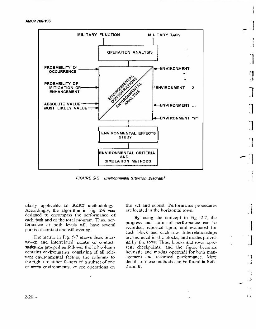
AMCP 706-196

MILITARY FUNCTION MILITARY TASK

OPERATION ANALYSIS

PROBABILITY CO- OCCURRENCE

PROBABILITY OF MITIGATION OR- ENHANCEMENT

ABSOLUTE VALUE- MOST LIKELY VALUE-

-ENVIRONMENT

'ENVIRONMENT 2

•-ENVIRONMENT ....

•—ENVIRONMENT "n"

ENVIRONMENTAL EFFECTS STUDY

ENVIRONMENTAL CRITERIA AND

SIMULATION METHODS

1 "1 ]

FIGURE 2-5. Environmental Sitwtion Diagram2

ularly applicable to PERT methodology. Accordingly, the algorithm in Fig. 2-6 was designed to encompass the performance of each task and of the total program. Thus, performance at both levels will have several points of contact and will overlap.

The matrix in Fig. ?-7 shows these interwoven and interrelated points of contact. Tasks are grouped as follows: the left column contains environments consisting of all relevant environmental factors; the columns to the right are either factors of a subset of one or more environments, or are operations on

the set and subset. Performance procedures are located in the horizontal rows.

By using the concept in Fig. 2-7, the progress and status of performance can be recorded, reported upon, and evaluated for each block and each row. Interrelationships are included in the blocks, and modes provided by the rows. Thus, blocks and rows represent checkpoints, and the figure becomes heuristic and modus operandi for both management and technical performance. More details of these methods can be found in Refs. 2 and 6.

J

2-20 J

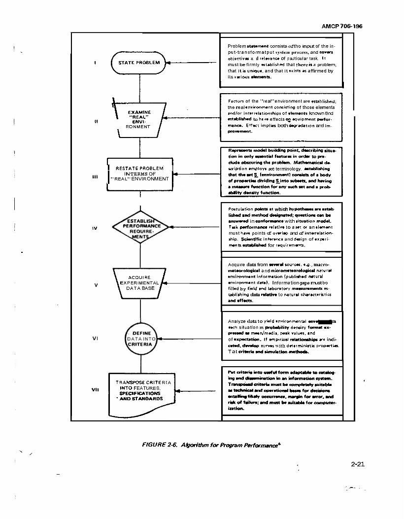
AMCP 706-196

I STATE PROBLEM \

\ EXAMINE "REAL"

ENVI RONMENT

III

RESTATE PROBLEM INTERMSOF

" REAL" ENVIRONMENT

IV

ACQUIRE {EXPERIMENTAL /ej-

DATA BASE

VI

VII

TRANSPOSE CRITERIA INTO FEATURES, SPECIFICATIONS

' AND STANDARDS

Problem tunmoni consists of tho input of the input-transformatput system process, and covers objectives a d relevance of particular task. It must be firmly estaolfshed that there«« problem, that it a unktue, and that it exists as affirmed by its various 4

Fjctors of the "real"environment are established; the realenvkonment consisting of those elements and/or interrelationships of elements known8nd established to have effects on equipment perfor- manca. Erf eel implies both degradation and im- pravffimrt.

Represents modal building point, describing situation in only essential features in order to pre- duda obscuring tha problem. Mathematical description employs set terminology, establishing that tha aat S_ (environment) consists of a body of properties dividing Sinto «uhaati. and having a measure function for any auch aat and a probability density function.

Postuiation points at which hypotheses ere estab- lishad and method daaignatad; questions can be answered i n conformance with situation model. Task performance relative to a sei or an element must have points <£ overlap and <£ intarralation- ship. Scientific inference and design of experiments established for requirements.

Acquire data from several sources, 14., macro- meteorological andmicrorneteorological ruturei environment information (published natural environment data). Information gaps mustbo filled by field and laboratory measurements establishing data relative to natural characteristics and effects.

Analyze data to yield environmental enve^p^î each situation m probability density format ax- pressed a« meerVmedit, peak values, and of expectation. If empirical relationships are indicated, develop curves with deterministic properties. T a t criteria and simulation methods.

Put criteria into useful form adaptable to catalog- ing and däsaammation in an information system. Tran ip need criteria must be completely suitable as technical and operetional bases for decisions einetting Nkaty occurrence, margin for error, and risk of failure; and must be auitaWa for computer- iaation.

FIGURE 2-6. Algorithm for Program Performance*'

2-21

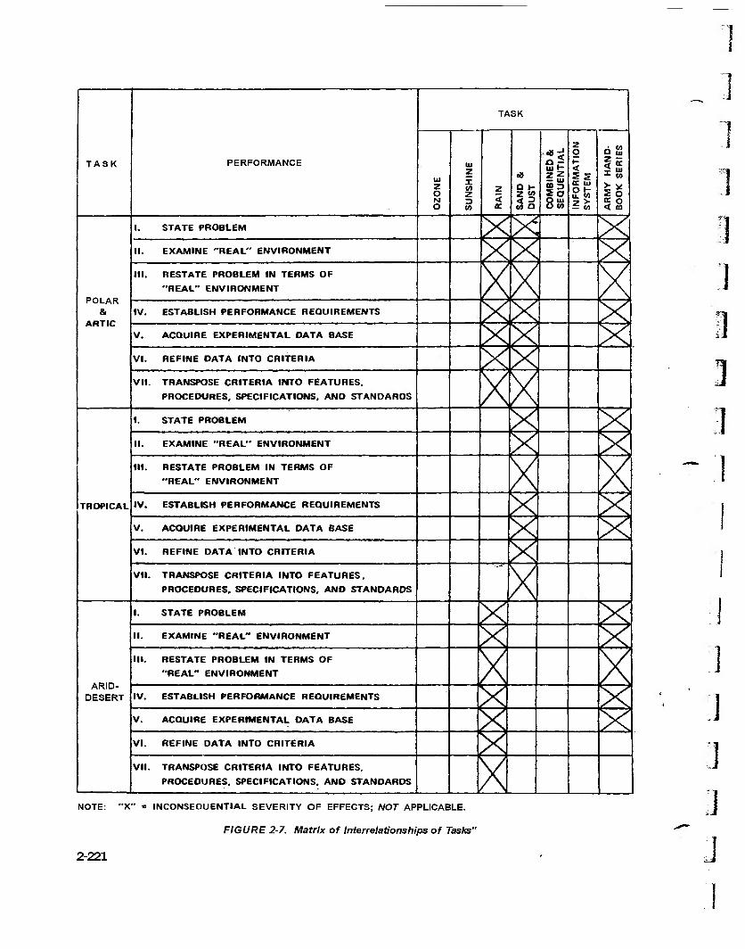
TASK PERFORMANCE

TASK

Ul Z o M o

Ul z I W z D

z 3 tc

O H z «» < 3 M Q

11 SO Q Ul O to IN

FO

RM

AT

ION

S

YS

TEM

0 ui

< K T Ul 1 CO

2 o 5 o

POLAR &

ARTIC

1. STATE PROBLEM

II. EXAMINE "REAL" ENVIRONMENT

III. RESTATE PROBLEM IN TERMS OF

"REAL" ENVIRONMENT

IV. ESTABLISH PERFORMANCE REQUIREMENTS

V. ACQUIRE EXPERIMENTAL DATA BASE

VI. REFINE DATA INTO CRITERIA

VII. TRANSPOSE CRITERIA INTO FEATURES.

PROCEDURES, SPECIFICATIONS. AND STANDARDS

TROPICAL

1. STATE PROBLEM



"REAL" ENVIRONMENT





PROCEDURES. SPECIFICATIONS. ANO STANDARDS

ARID- DESERT

1. STATE PROBLEM



"REAL" ENVIRONMENT





PROCEDURES. SPECIFICATIONS. ANO STANDARDS

0

;]

NOTE: "X" * INCONSEQUENTIAL SEVERITY OF EFFECTS; NOT APPLICABLE.

FIGURE 2-7. Matrix of Interrelationships of Tasks"

}

]

2-221

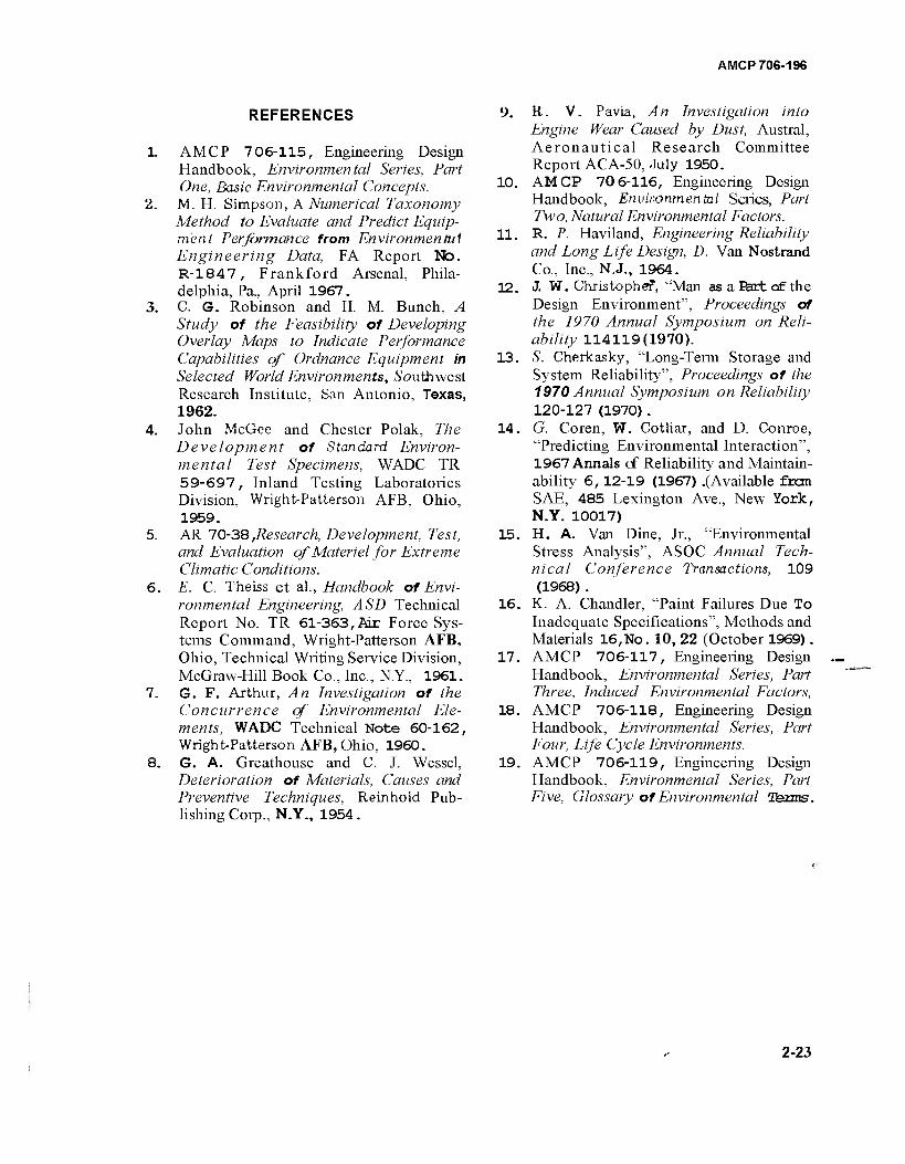
AMCP 706-196

REFERENCES

1. AMCP 706-115, Engineering Design Handbook, Environmental Series, Part One, Basic Environmental Concepts.

2. M. H. Simpson, A Numerical Taxonomy Method to Evaluate and Predict Equip- ment Performance from Environment Engineering Data, FA Report No. R-1847, Frankford Arsenal, Phila- delphia, Pa, April 1967.

3. CG. Robinson and H. M. Bunch, A Study of the Feasibility of Developing Overlay Maps to Indicate Performance Capabilities of Ordnance Equipment in Selected World Environments, Southwest Research Institute, San Antonio, Texas, 1962.

4. John McGee and Chester Polak, The Development of Standard Environ- mental Test Specimens, WADC TR 59-697, Inland Testing Laboratories Division, Wright-Patterson AFB, Ohio, 1959.

5. AR 70-38 ,Research, Development, Test, and Evaluation of Materiel for Extreme Climatic Conditions.

6. E. C. Theiss et al., Handbook of Envi- ronmental Engineering, ASD Technical Report No. TR 61-363,Air Force Sys- tems Command, Wright-Patterson AFB, Ohio, Technical Writing Service Division, McGraw-Hill Book Co., Inc., N.Y., 1961.

7. G. F. Arthur, An Investigation of the Concurrence of Environmental Ele- ments, WADC Technical Note 60-162, Wright-Patterson AFB, Ohio, 1960.

8. G. A. Greathouse and C. J. Wessel, Deterioration of Materials, Causes and Preventive Techniques, Reinhold Pub- lishing Corp., N.Y., 1954.

9. R. V. Pavia, An Investigation into Engine Wear Caused by Dust, Austral, Aeronautical Research Committee Report ACA-50, July 1950.

10. AMCP 70 6-116, Engineering Design Handbook, Environmental Series, Part Two, Natural Environmental Factors.

11. R. P. Haviland, Engineering Reliability and Long Life Design, D. Van Nostrand Co., Inc., N.J., 1964.

12. J. W. Christopher, "Man as a Eört afthe Design Environment", Proceedings of the 1970 Annual Symposium on Reli- ability 114119(1970).

13. S. Cherkasky, "Long-Term Storage and System Reliability", Proceedings of the 1970 Annual Symposium on Reliability 120-127 (1970).

14. G. Coren, W. Cotliar, and D. Conroe, "Predicting Environmental Interaction", 1967 Annals cf Reliability and Maintain- ability 6,12-19 (1967) .(Available fron SAE, 485 Lexington Ave., New York, N.Y. 10017)

15. H. A. Van Dine, Jr., "Environmental Stress Analysis", ASOC Annual Tech- nical Conference Transactions, 109 (1968).

16. K. A. Chandler, "Paint Failures Due To Inadequate Specifications", Methods and Materials 16,No. 10, 22 (October 1969).

17. AMCP 706-117, Engineering Design Handbook, Environmental Series, Part Three, Induced Environmental Factors,

18. AMCP 706-118, Engineering Design Handbook, Environmental Series, Part Four, Life Cycle Environments.

19. AMCP 706-119, Engineering Design Handbook, Environmental Series, Part Five, Glossary of Environmental Terms.

2-23

AMCP 706-196

CHAPTER 3 MEASURES OF RELIABILITY

3-0 LIST OF SYMBOLS

Cdf = Cumulative distribution function MTBF = mean time between failures MTTF = mean time to failure

pdf = probability density function Sf = Survivor function, Sf = 1 — Cdf

t = time to failure (for nonrepairable items) time between failures (for repairable items)

3 1 INTRODUCTION

Engineers face tremendous difficulties in attempting to measure reliability, maintainability, safety, or other product characteristics precisely with a single number. The reason for the difficulty is that products are usually complex, are made up of many different parts, serve many different uses, and operate under many different conditions. The question "how good is a jeep?" might well take 50 pages of explanation and great detail to arrive at a plethora of answers. How then is it possible to measure the reliability of ajeep with a single number?

By using a single number to measure reliability, some information is lost, But the con- venience of one number—or perhaps a few numbers-makes up for the lost information. All the measures given in this chapter are related to probabilities. The methods for calculating (predicting) reliability are given in Part Three, Reliability Prediction. A discussion of many concepts in probability and statistics together with information about specific probability distributions are given in Part Six, Mathematical Appendix and Glos- sary. Techniques involved in estimating and measuring reliability by means of test results on existing items are given in Part Four, Reli- ability Measurement,

The process of designing, creating, and producing reliable hardware is an engineering one, not a statistical one. But the measures of reliability are statistical; so the engineer does need to be familiar with probability and statistics.

Reliability is a measure of the ability of an item to complete its mission successfully,

given that the item was in proper condition (available) at the mission beginning. Some- times, quantitative reliability measures are assigned as a goal in -the conceptual stage, before any design or hardware has been fabricated. In this case, the system must be designed and the subsystems and parts selected to preserve the desired reliability. At each decision point in the concept, design, or fabrication phase, the system reliability must be predicted. In these cases, the predicted reliability is compared with the required reliability, and such changes and trade-offs made as are necessary. This reliability constraint imposed upon designers and developers of equipment is not different in spirit from the cost constraints imposed on an architect. He wishes to create as distinguished a building as possible within the limits of his allowed costs. Nor is it different in spirit from the weight constraints imposed on an aircraft designer who must consider engine, equipment, and fuel requirements against the weight of the payload. The difference with the constraint on reliability is that it has been more recently recognized. Reliability, like cost and weight, must be specified in advance; the quantitative measures of reliability make it possible to do this.

Of the several measures of reliability, it is a matter of engineering judgment to decide which to use. Mair/ ties it will make little difference, but sometimes it will. A supplier, once given the measure as a specification, might well try to maximize his gains by changing anything but the specified measure. Se&Part Five, Caatzactingfor Reliability.

3-2 PROBABILITIES OF SUCCESS AND FAILURE

The traditional narrow definition of reli-, ability as a probability of success is repeated ' here from par. 1-1:

"s-Reliability is the probability that an item \ÖIL perform its intended function for a specific interval under stated conditions."

This definition has two major shortcomings:

3-1

AMCP 706-196

(l)It does not cover one-shot items like ammunition.

(2) It does not explicitly consider the condition of the item at the beginning of the mission, whereas virtually all calculations and predictions of s-reliability do consider it.

Most of the theoretical analyses of reliability which appear in the literature and those in Part Three, Reliability Prediction use the following definition which alleviates those two shortcomings:

"s-Reliability is the probability that an item successfully completes its mission, given that the item was in proper condition at the beginning of the mission."

In a practical situation, the four elements of the definition must be carefully explained, defined, and delineated.

(1) The item (2) The mission (especially any limita-

tions on repair during the mission) (3) Successful completion (4) Proper condition (especially the

manner in which it is assured).

For a theoretical analysis one usually specifies the repair philosophy for the components during the mission, and in what conditions the components may appear during the mission. Proper-condition almost always is assumed to be "every component is good", not merely that the item is functioning.

One-shot items are covered in par. 3-7.

The probability cf failure often is calculated, rather than probability of success, because of the significant-figure difficulty with probabilities near 1 and because of the easy approximations for small probabilities. Failure and success are complementary events; the sum of their probabilities is 1.

3-3 FAILURE DISTRIBUTIONS

A failure distribution gives all the information about times to failure, not just a single number. (This paragraph is written as if the variable of interest is failure-time, but the variable could easily be strength, damage,

] etc.) In the usual application of failure distributions it is presumed that no failure/repair pairs are allowed, although preventive maintenance is considered occasionally. The statistical concepts of failure distributions are explained in Part Six, Mathematical Appendix and Glossary, The probability density function (pdf) is the description of a distribution most often used in discussions. It historically has been used, it has mathematical conveni- ence, and its shape is usually quite characteristic of the distribution (whereas all cumulative distribution functions tend to look alike). It will be used in this paragraph. The uses of failure distributions are classified conveniently into interpolation, extrapolation, and calculations of moments and percentiles.

Interpolation (usually a smoothing type) means calculating a value of the pdf for a failure time that is within the region where data are available, but for which there was no test result or for which some smoothing of data was needed. The choice of failure distribution is not critical in interpolation. Many distributions will give equally good results, especially when goodness is evaluated with respect to the usual tremendous uncertainty in the data

Extrapolation means calculating a value of thepdf for a failure time that is outside the region where data are available. This is the most popular and the most misleading use of distributions. It is misleading because the user forgets that he doesn't know the behavior in this region; he then confuses "numerical precision in calculation" with "accuracy of describing the real behavior". One method cf avoiding this trap is to use two regions of failure time: internal and external. The internal region is essentially the one where interpolation, or very mild extrapolation, is possible. The external region is the one where gross extrapolation would have to be used. Very often it will be in two parts, one on either side of the internal region. One then estimates the fraction of the population which lieswith- in these two subregions. In any subsequent calculation, a further assumption might have to be made about where in the subregionthe values might be; but then the user is on guard that he is guessing and that he should see what happens for several different guesses, There is absolutely no law of nature that says

J

1

3-2

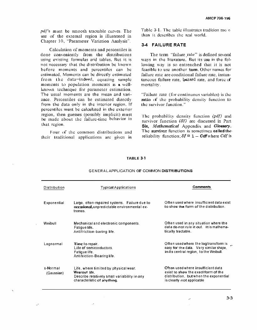
AMCP 706-196

pdf's must be smooth tractable curves. The use of the external region is illustrated in Chapter 10, "Parameter Variation Analysis".

Calculation of moments and percentiles is done conveniently from the distributions using existing formulas arid tables. But it is not necessary that the distribution be known before moments and percentiles can be estimated, Moments can be directly estimated from the data—indeed, equating sample moments to population moments is a well- known technique for parameter estimation. The usual moments are the mean and variance. Percentiles can be estimated directly from the data only in the interior region. If percentiles must be calculated in the exterior region, then guesses (possibly implicit) must be made about the failure-time behavior in that region.

Four of the common distributions and their traditional applications are given in

Table 3-1. The table illustrates tradition mo e than it describes the real world.

3-4 FAILURE RATE

The term "failure rate" is defined several ways in the literature. But its use in the following way is so entrenched that it is not feasible to use another term. Other names for failure rate are conditional failure rate, instantaneous failure rate, b«zard rate, and force of mortality.

"Failure rate (for continuous variables) is the ratio of the probability density function to the survivor function."

The probability density function (pdf) and survivor function (Sf) are discussed in Part Six, Mathematical Appendix and Glossary. The survivor function is sometimes called the reliability function; Sf= 1 — Cdfwhere Cdf is

TABLE 3-1

GENERAL APPLICATION OF COMMON DISTRIBUTIONS

Distribution Typical Applications Comments

Exponential Large, often-repaired systems. Failure due to occasional,unpredictable environmental extremes.

Often used where insufficient data exist to show the form of the distribution.

Weibull Mechanical and electronic components. Fatigue life. Antifriction-baring life.

Often used in any situation where the data do not rule it out. Itis mathematically tractable.

Lognormal Time to repair. Life of semiconductors. Fatigue life. Antifriction-Bearing life.

Often usedwhere the log transform is easy for the data. Very similar shape, in its central region, to the Weibull.

s-Normal (Gaussian)

Life, where limited by physical wear. Wearout life. Describe relatively small variability inany characteristic of anything.

Often usedwhere insufficient data exist to show the exact form of the distribution, butwhen the exponential is clearly not applicable

3-3

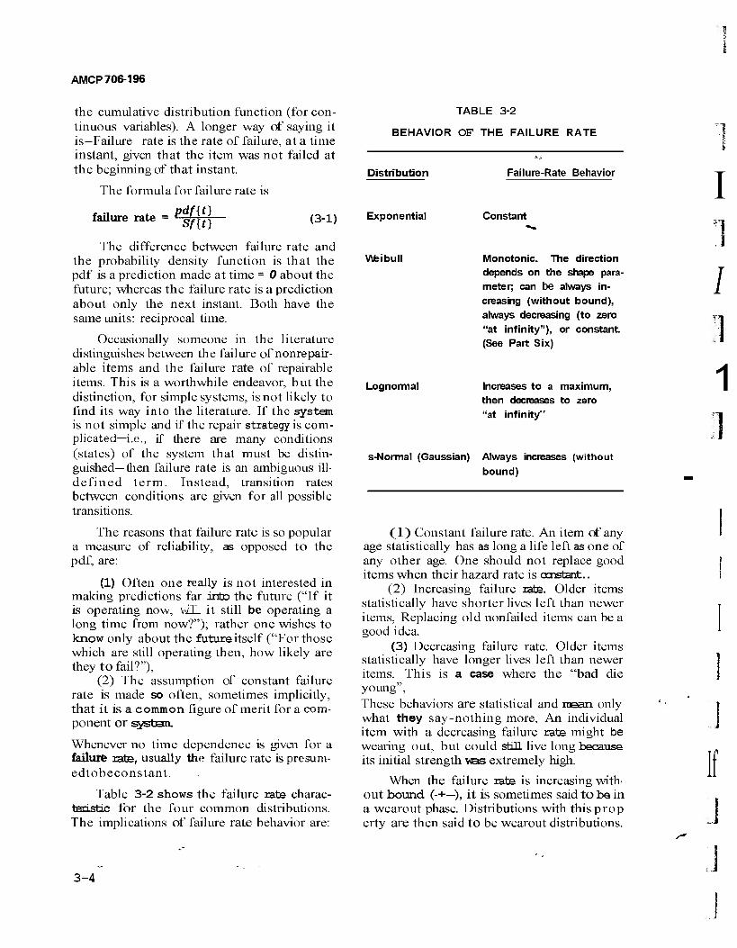
AMCP 706-196

the cumulative distribution function (for continuous variables). A longer way of saying it is-Failure rate is the rate of failure, at a time instant, given that the item was not failed at the beginning of that instant.

TABLE 3-2

BEHAVIOR OF THE FAILURE RATE

The formula for failure rate is

failure rate pdfjt}

Sf{t] (3-1)

The difference between failure rate and the probability density function is that the pdf is a prediction made at time = 0 about the future; whereas the failure rate is a prediction about only the next instant. Both have the same units: reciprocal time.

Occasionally someone in the literature distinguishes between the failure of nonrepairable items and the failure rate of repairable items. This is a worthwhile endeavor, but the distinction, for simple systems, is not likely to find its way into the literature. If the system is not simple and if the repair strategy is complicated—i.e., if there are many conditions (states) of the system that must be distinguished—then failure rate is an ambiguous ill- defined term. Instead, transition rates between conditions are given for all possible transitions.

The reasons that failure rate is so popular a measure of reliability, as opposed to the pdf, are:

(1) Often one really is not interested in making predictions far into the future ("If it is operating now, WH_ it still be operating a long time from now?"); rather one wishes to know only about the future itself ("For those which are still operating then, how likely are they to fail?"),

(2) The assumption of constant failure rate is made so often, sometimes implicitly, that it is a common figure of merit for a component or system.

Whenever no time dependence is given for a failure rate, usually tho failure rate is presum- edtobeconstant.

Table 3-2 shows the failure rate characteristic for the four common distributions. The implications of failure rate behavior are:

Distribution

Exponential

Weibull

Failure-Rate Behavior

Lognormal

Constant

Monotonie. The direction depends on the shape parameter; can be always increasing (without bound), always decreasing (to zero "at infinity"), or constant. (See Part Six)

Increases to a maximum, then decreases to zero "at infinity"

s-Normal (Gaussian) Always increases (without bound)

(1) Constant failure rate. An item of any age statistically has as long a life left as one of any other age. One should not replace good items when their hazard rate is omstant..

(2) Increasing failure rate. Older items statistically have shorter lives left than newer items, Replacing old nonfailed items can be a good idea.

(3) Decreasing failure rate. Older items statistically have longer lives left than newer items. This is a case where the "bad die young", These behaviors are statistical and mean only what they say-nothing more, An individual item with a decreasing failure rate might be wearing out, but could stül live long because its initial strength was extremely high.

When the failure rate is increasing without bound (-+—), it is sometimes said to be in a wearout phase. Distributions with this prop erty are then said to be wearout distributions.

I

/

1 D

If J

3-4

AMCP 706-196

The s-normal (Gaussian) and some Weibull distributions are wearout distributions. The exponential and lognormal distributions are not.

The parameter of a Poisson process is also a failure rate. See Refs, 1 or 2 for more details.

The failure rate of a system is often fairly high at the beginning when it is put into commission. This is largely due to human frailty in one form or another. Then, once the severe weaknesses have been removed (possibly even by redesign) the failure rate often settles down to a reasonably constant value (fluctuates within a factor of 2 or so). Some systems, if they are used long enough, have a rise in failure rate because many of the components seem to near the end of their useful lives. If this failure rate behavior is plotted as a function of time, it has the so-called bathtub shape. Many electronic systems become obsolete before their failure rate rises appreciably. Some systems are debugged thoroughly before being delivered. The bathtub curve is neither inevitable nor always desirable. It is better to avoid the term and separately discuss variations in failure rate if they will be important.

3-5 TIME-TO-FAILURE

This concept applies to nonrepairable items. It is sometimes called time-to-first- failure, but that concept usually is confusing since further failures are implied, but yet time-between-failures is obviously not meant. (One can, of course, calculate and use any figure he chooses, provided both he and the intended reader understand it.) In this paragraph, each item fails but once and so "failure" is "first failure", If the item is repaired and returned to a like-new condition, then it is considered a different, new item.

Not all failure-time distributions have a mean (i.e., the mean is "infinite"), but the usual ones do. The mean time-to-failure MT TF is

MTTF 'f t Pdf{t\dt = L Sf{t\dt 0 (3-2)

if the MTTF exists; where

t = time to failure pdf = probability density function

Sf = survivor function

The MTTF is used because it is tractable and traditional. In some instances, the existence of many long-lived items inflates the MTTF so that it is not characteristic of lives actually observed in the field. Very often a median time-to-failure is more characteristic of the lives that will be observed in the field. For short times, failure rate is often a better, more useful reliability measure than MTTF; the early failures will hurt the system—no one cares about the exact life of the very long- lived systems.

The means and medians of the common distributions are given in Part Six, Mathemati- cal Appendix and Glossary.

3-6 TIME BETWEEN FAILURES

This concept applies to' repairable items, In any repair situation one must know the presumed condition of the item after repair in order to make calculations. There are two conventional tractable assumptions:

(1)A repaired item is "good as new". This means that, statistically, the repaired item is just like anew one.

(2) A repaired item is "bad as old". This means that, statistically, the repaired item is just as bad as it was before failure. An example is a jeep, just after a failed set of distributor points has been replaced; the overall condition of the jeep has not been significantly altered by the repair.

If the failure rate is constant, then the two assumptions are equivalent, since age is irrele- vant in predicting future life.

When the repaired item is "good as new",' the time-between-failures is the same as time- , to-failure, If not, then the repair philosophy must be explicitly enumerated.

The mean time-between-failures (MTBF) appears often in the reliability literature; it is defined just as in Eq. 3-2. Unfortunately, the repair situation is rarely explained. In some

3-5

AMCP 706-196

cases, the author may have been confused and, if it is a theory paper, the author may not even realize what his implicit assumptions are. Virtually always when MTBF is given a specific value (e.g., MTBF = 100 hr), the failure rate of the item is presumed constant (or reasonably s^. When failure rate is constant, the MTBF is just the reciprocal of the failure rate.

For large complex repairable systems where no few components are responsible for many of the failures, and where the system has had many failures already, the failure rate is reasonably constant and MTBF is a reasonable concept.

Theoreticians have to be more wary of this concept than do engineers.

3-7 FRACTION DEFECTIVE

For one-shot items, such as ammunition, the time concept in reliability is not appropriate. They either function, or they fail in some way. So the fraction defective (or fraction good) is a useful concept. One often wishes to classify failures into several categories. For ammunition, twocommon categories are duds and prematures; generally, the fraction of prematures should be much less than the fraction of duds.

Another case where fraction defective ib appropriate is where a distribution ofstrength of an item is reasonably known between some limits; e.g., the strength has an s-normal distribution with mean 10,000 ID and standard deviation of 1000 lb, in the range 7000 to 13000 lb. On the weak side, the actual strength is not known, the items are just considered defective and the fraction defective is estimated, say 0.5%. One rarely will care if a small fraction has strengths above 13000 !b because they will not affect appreciably the reliability.

Another use for fraction defective is where one doesn't care how good an item is, or how long it lasts, just as long as it is good enough. Then those which are good enough constitute the fraction good; the others are the fraction defective.

REFERENCES

W. Feller, An Introduction to Probability Theory and its Applications, John Wiley and Sons, Inc., N.Y., 1966. M. L. Shooman, Probabilistic Reliability: An Engineering Approach, McGraw-Hill Book Co., N.Y., 1968.

1

3-6

CHAPTER 4 MODEL BUILDING AND ANALYSIS

4-0 LIST OF SYMBOLS

Cdf = Cumulative distribution function

f(t) = pdf{t) f(x) = pdf{x]

F(x) = Cdf{x) g(y) = pdf{y) G(y) = Cdf{y) pdf = probability density function

R(t) = Sf{t} Sf = Survivor function, Sf = 1 — Cdf

t = a random variable, time X = any random variable y = F(x) a = scale parameter, see Table 4-1 ß = shape parameter, see Table 4-1 X = a failure rate

4-1 INTRODUCTION

No one can analyze the real world situation or the real hardware; he can only analyze his mental picture of the situation or hardware. This mental picture is called a conceptual model (often shortenedjust to "model").

The idea of a conceptual model is adapted from the idea of a physical model such as a model car. In a physical model, the characteristics of importance are reproduced quite well. In a model car these might be propor- tions, shape, and color. The characteristics of little or no importance are not usually reproduced at all; e.g., there may be no motive power and the tires may not be pneumatic. The "inbetweens" receive indifferent treatment. The physical model is an abstracting of something important from the physical world; it is an imitation.

A conceptual model is analogous to a physical model. Since everything in the universe affects everything else to some degree, however slightly, any exact treatment would be hopelessly complicated. Therefore the engineer decides how he will look at the situation and makes a set of assumptions (both explicit and implicit) about what he will ignore and what he will include in the conceptual model. By its very nature, a con-

ceptual model is incomplete: it ignores some things and describes others in an approximate fashion.

After having made,a set cf assumptions for a conceptual model, the engineer then operates on those assumptions with mathematics and logic; he analyzes them by any means at his disposal. While developing the logical implications »I a set of assumptions, he often doesn't like the results: they don't seem to fit; they appear to be inconsistent with his beliefs, etc. Then he has two rational choices:

(1) Change his beliefs about the way the world is, if he is convinced that the set of assumptions is very realistic; and/or

(2) Go back and modify the assumptions, so that their logical implications do in fact fit his beliefs about the world.

The creation of a conceptual model is a cir- cular, often haphazard, process wherein ideas come from everywhere and get analyzed, tested, compared, junked, and accepted.

A conceptual model is often mathematical in nature and the same formalism will describe several different situations. It is important to keep the distinction between the mathematics itself (which is quite general, completely impersonal, and always "true") and what it represents in an engineering sense.

All reliability analyses and optimizations are made on conceptual models of equipment, not on the equipment itself. The engineer forgets this at the peril of the person in the field who uses, not the engineer's conceptual model, but the real hardware.

This chapter describes the procedure used to create mathematical models of systems. The models can then be analyzed by the methods in Part Three. Reliability Prediction.

For systems with (a)repair, and (b) many elements that are treated separately, a more complicated description is needed than for simple nonrepairable systems. The possible states (conditions) of each element are defined, and the state (condition) of the system is the set of states of the elements. This

4-1

AMCP 706-196

approach is sometimes called the state-matrix approach because the state of the system is described, not by a single number, but by a matrix of numbers. The approach is discussed more fully in par. 4-2.

Some terms that will be used are defined:

(1) Element. An element of a system is an item whose failure and repair characteristics are considered as a unit and not as a collection of items.

(2) Up. An item is up if it is capable of performing its function; i.e., it is available. There might be various degrees of being up, each with different failure behavior.

(3) Down, An item is down if it is not up.

(4) On. An item is on if it is both up and operating.

(5) Idle. An item is idle if it is up and not operating; i.e., it is being held in standby.

(6) State. The state of an item is a statement of its condition, as measured by its characteristics which are considered important. The states are often given names such as Up, In Repair, Degraded, Standby, or Failed.

'(7) State-matrix. The state-matrix of an item is the matrix of the states of the elements of the item.

(8) Series. Elements of a subsystem are in series if they all must be up for the subsystem to be up,

4-2 MODEL BUILDING

To compute the reliability and maintainability measures of a system, there must be a mathematical model of the system. The appropriate mathematical model is a reliability model which aonsists cf a reliability block diagram or a Cause-Consequence chart; all equipment failure time and repair t i e distributions; a definition cf the states of each element and of the item; and a statement of maintenance, spares, and repair strategies,

A reliability, block diagram is obtained from a careful analysis of the manner in which the system operates—i.e., the effects of failures on overall system performance cf the various parts that make up the system; the support environment and constraints including such factors as the number and assignment

cf spare parts and repairmen; and finally, a consideration of the mission to be performed by the system. Careful consideration of these aspects yields a set of rules (which will be referred to as up-state rules) which define satisfactory operation of the system (system up) and unsatisfactory operation (system down), as well as the various ways in which these can be achieved. If a system operates in more than one mode, a segarate reliability diagram must be developed for each.

For complicated systems, a Cause- Consequence chart might be more appropriate than a reliability diagram. See Chapter 7 for a discussion cf Cause-Consequence charts and fault trees. Regardless of which is used, the model building is similar. This chapter uses reliability diagrams because the discussion is simpler that way.

A considerable amount of engineering analysis must be performed in order to develop a reliability model. The engineering analysis proceeds as follows:

(l)The engineer develops a functional block diagram of the system based on his knowledge of the physical principles governing system operation.

(2) The engineer uses the results of performance evaluation studies to determine to what extent the system can operate in a degraded state. This information can be provided by outside sources.

(3) Eased on the functional block diagram, and the amount of acceptable perfonnance degradation, the engineer develops the reliability block diagram, and the upstate rules.

(4) The reliability block diagram and the upstate rules are used as inputs to the equations for system behavior and for calculating various measures of reliability and maintainability (including availability). The actual analyses are described in Part Three, Reliability Prediction,

The reliability diagram is a pictorial way of showing all the success or failure combinations of the blocks in the system, Those combinations must be known before the reliability diagram can be drawn; one does not "derive" the combinations from the diagram for the first time; rather, they are implicit in

4-2

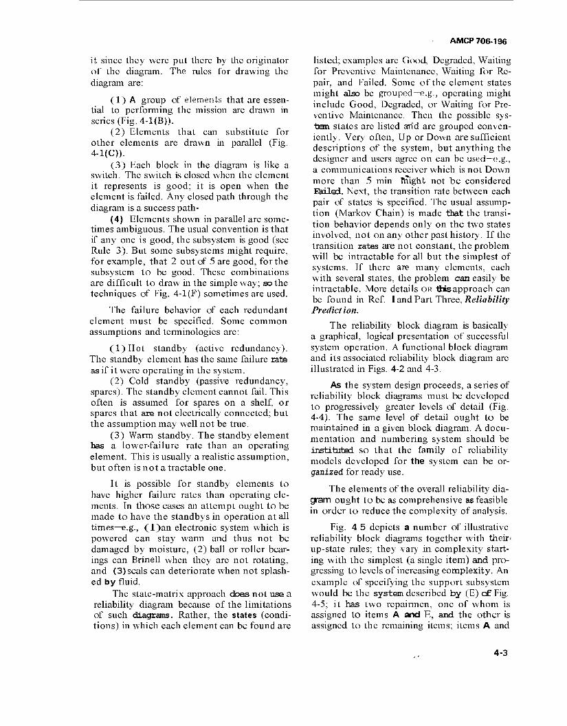
AMCP 706-196

it since they were put there by the originator of the diagram. The rules for drawing the diagram are:

(1) A group of elements that are essential to performing the mission are drawn in series (Fig. 4-l(B)).

(2) Elements that can substitute for other elements are drawn in parallel (Fig. 4-KC)).

(3) Each block in the diagram is like a switch. The switch is closed when the element it represents is good; it is open when the element is failed. Any closed path through the diagram is a success path-

(4) Elements shown in parallel are sometimes ambiguous. The usual convention is that if any one is good, the subsystem is good (see Rule 3). But some subsystems might require, for example, that 2 out of 5 are good, for the subsystem to be good. These combinations are difficult to draw in the simple way; so the techniques of Fig. 4-1 (F) sometimes are used.

The failure behavior of each redundant element must be specified. Some common assumptions and terminologies are:

(l)Hot standby (active redundancy). The standby element has the same failure rate as if it were operating in the system.

(2) Cold standby (passive redundancy, spares). The standby element cannot fail. This often is assumed for spares on a shelf, or spares that are not electrically connected; but the assumption may well not be true.

(3) Warm standby. The standby element has a lower-failure rate than an operating element. This is usually a realistic assumption, but often is not a tractable one.

It is possible for standby elements to have higher failure rates than operating elements. In those cases an attempt ought to be made to have the standbys in operation at all times—e.g., (l)an electronic system which is powered can stay warm and thus not be damaged by moisture, (2) ball or roller bearings can Brinell when they are not rotating, and (3) seals can deteriorate when not splash- ed by fluid.

The state-matrix approach does not use a reliability diagram because of the limitations of such diagrams. Rather, the states (conditions) in which each element can be found are

listed; examples are Good, Degraded, Waiting for Preventive Maintenance, Waiting for Re- pair, and Failed. Some of the element states might also be grouped—e.g., operating might include Good, Degraded, or Waiting for Pre- ventive Maintenance. Then the possible system, states are listed arid are grouped conveniently. Very often, Up or Down are sufficient descriptions of the system, but anything the designer and users agree on can be used—e.g., a communications receiver which is not Down more than 5 min might not be considered E=ri1ad. Next, the transition rate between each pair of states is specified. The usual assumption (Markov Chain) is made that the transition behavior depends only on the two states involved, not on any other past history. If the transition rates are not constant, the problem will be intractable for all but the simplest of systems. If there are many elements, each with several states, the problem can easily be intractable. More details OR this approach can be found in Ref. land Part Three, Reliability Prediction.

The reliability block diagram is basically a graphical, logical presentation of successful system operation. A functional block diagram and its associated reliability block diagram are illustrated in Figs. 4-2 and 4-3.

As the system design proceeds, a series of reliability block diagrams must be developed to progressively greater levels of detail (Fig. 4-4). The same level of detail ought to be maintained in a given block diagram. A documentation and numbering system should be instituted so that the family of reliability models developed for the system can be or- ganized for ready use.

The elements of the overall reliability diagram ought to be as comprehensive as feasible in order to reduce the complexity of analysis.

Fig. 4 5 depicts a number of illustrative reliability block diagrams together with their' up-state rules; they vary in complexity starting with the simplest (a single item) and pro- gressing to levels of increasing complexity. An example of specifying the support subsystem would be the system described by (E) cf Fig. 4-5; it has two repairmen, one of whom is assigned to items A and E, and the other is assigned to the remaining items; items A and

4-3

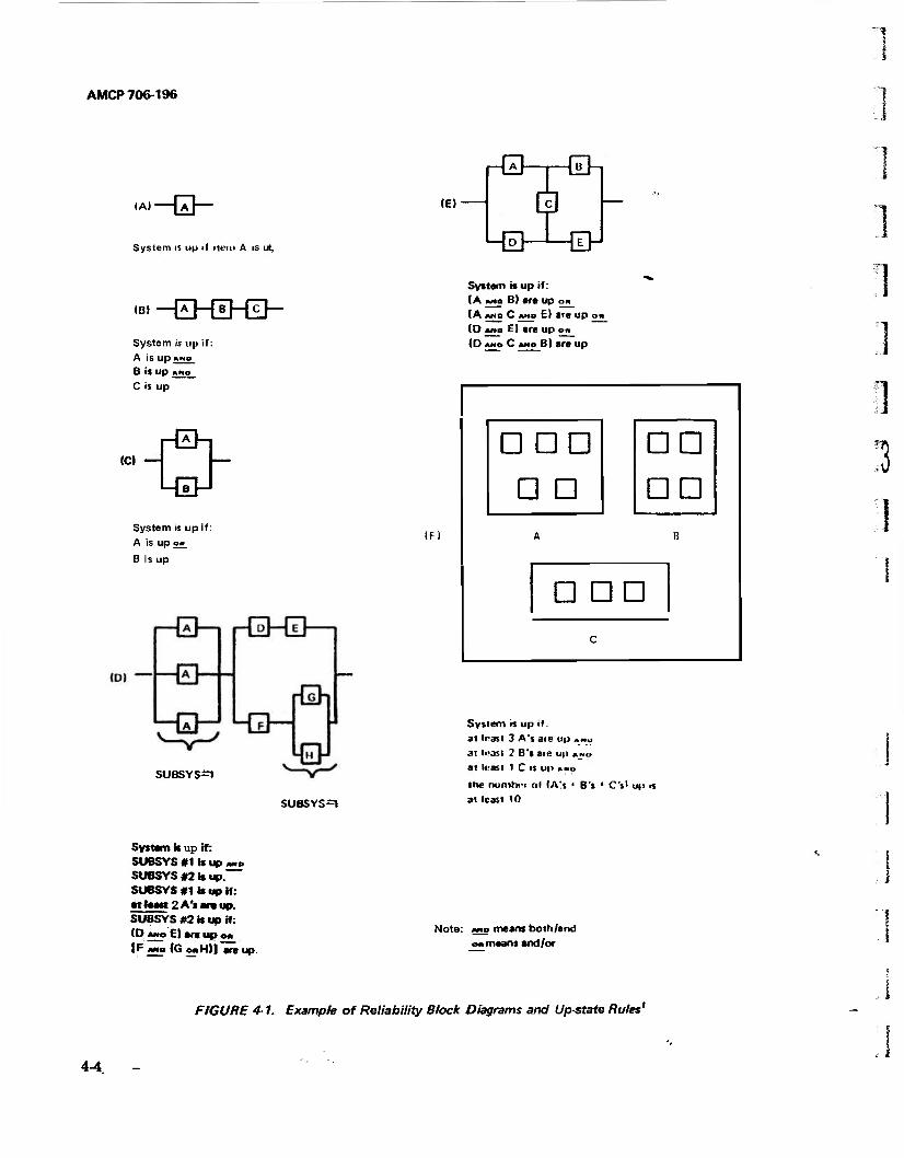
AMCP 706-196

(Al—0—

System is up <l HKM A IS ut,

IE)

r-0-T-S-i

LQ_L_[7}J

(Bl -EKEH3- System is up if: A is up »wo B is up AMO

C is up

<C| —

-0- System is up if: A is up on

B is up

SUBSYS=1

(F)

System it up if:

(A MO B) are up o»_ (A AMo C AMo E) are up o*_ (D AMD E) are up on_ (D AMo C AMD B) are up

DDD D D

DD DD

A B

DDD c

SUBSYS=l

System is up if at least 3 A's aie up *«» at li'asi 2 B's ate up »~i> at leasi 1 C is up »»o

the numhi'i ol (A's * 8's * C's' up is at least 10

3

System it up if: SUBSYS #1 is up AMP

SUBSYS #2 Is up. SUBSYS #1 to up it: atjaatt 2 A't at» up. SUBSYS #2 it up if: (O MO E) are up ©«_

IF «» (G MHI] are up.

Note: MO meant both/and »■means and/or

FIGURE 4-1. Example of Reliability Block Diagrams and Up-state Rules'

4-4.

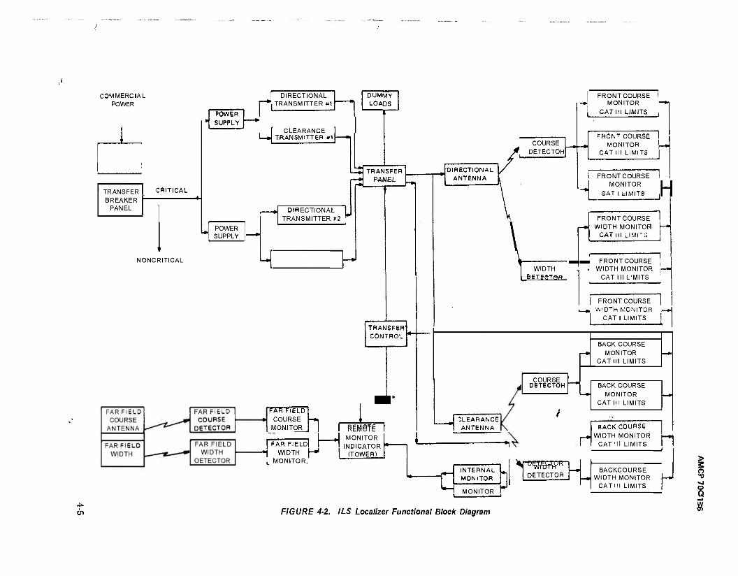
COMMERCIAL POWER

TRANSFER BREAKER

PANEL

CRITICAL

POWER SUPPLY

POWER SUPPLY

NONCRITICAL

n DIRECTIONAL

TRANSMITTER #1

CLEARANCE TRANSMITTER «1

DUMMY LOADS

DIRECTIONAL TRANSMITTER #2 V

COURSE DETECTOH

TRANSFER PANEL

TRANSFER CONTROL

FAR FIELD COURSE -*.

MONITOR J I I RiM§TE r————1 | J MONITOR [FAR FIELD] | | |ND|CATOR

-^ WIDTH (-• (TOWER) MONITOR,

DIRECTIONAL ANTENNA

FRONT COURSE -J MONITOR

CAT III LIMITS

WIDTH _BETggTSR,..

FRONT COURSE MONITOR

CAT III LIMITS

FRONTCOURSE MONITOR

SAT I fclMlTS

FRONTCOURSE WIDTH MONITOR

CAT III L.IMH ij

CLEARANCE ANTENNA

COURSE DETECTOH

BACK COURSE MONITOR

CAT III LIMITS

BACK COURSE MONITOR

CAT III LIMITS

n BACK COURSE

WIDTH MONITOR CAT III LIMITS

□ MONITOR \

K»r\Kl ITHD MONITOR

ÎTJT'R^ DETECTOR

BACKCOURSE WIDTH MONITOR

CAT III LIMITS

FIGURE 4-2. ILS Localizer Functional Block Diagram

H

^ FRONTCOURSE J WIDTH MONITOR

CAT III LIMITS

FRONTCOURSE | WIDTH MONITOR -

CAT I LIMITS j

r > o T3

O Q

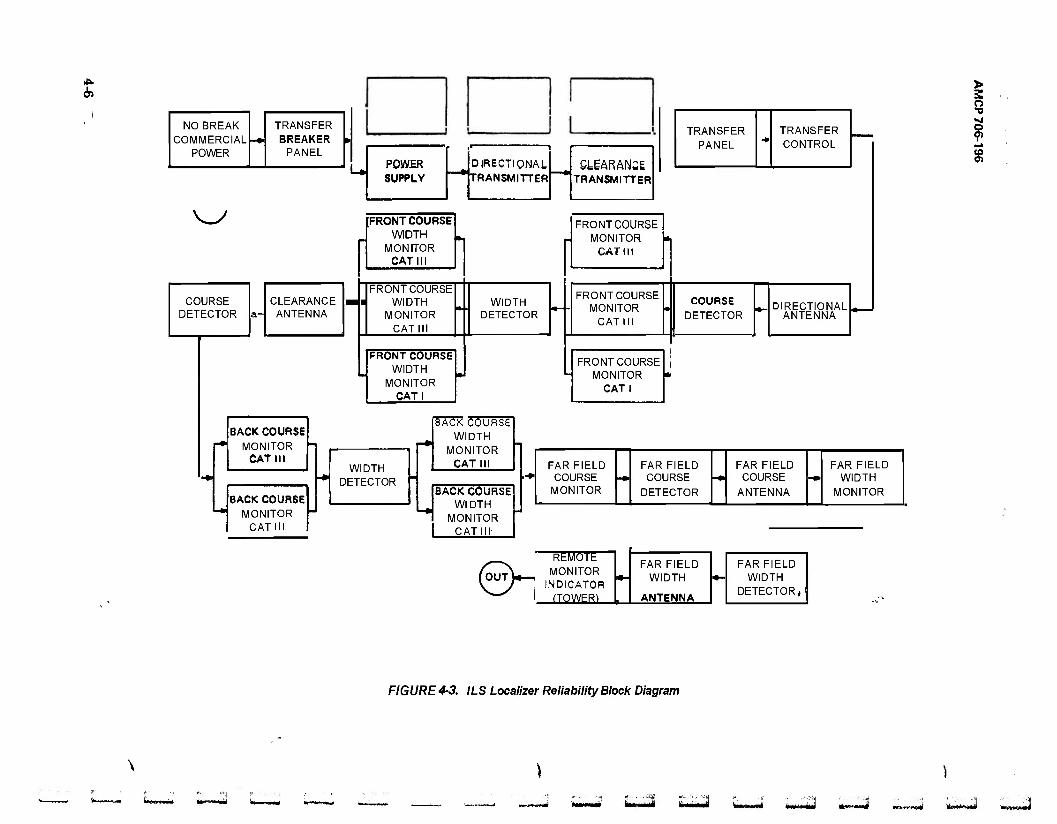
itfc

6>

NO BREAK COMMERCIAL

POWER

TRANSFER BREAKER

PANEL POWER SUPPLY

■ ■ i

DIRECTIONAL TRANSMITTER

CLEARANCE TRANSMITTER

TRANSFER PANEL ■*

TRANSFER CONTROL

w

COURSE DETECTOR

CLEARANCE ANTENNA

[FRONT COURSE WIDTH

MONFOR CAT III

FRONT COURSE WIDTH

MONITOR CAT III

FRONT COURSE WIDTH

MONITOR CAT I

WIDTH DETECTOR


CAT III


CAT III


CAT I

COURSE DETECTOR

DIRECTIONAL ANTENNA

> s o

?

BACK COURSE MONITOR

CAT III

BACK COURSE MONITOR

CAT III

WIDTH DETECTOR

l£c"R couflse WIDTH

MONITOR CAT III

BACK COURSE WIDTH

MONITOR CAT III

FAR FIELD COURSE MONITOR

- FAR FIELD COURSE

DETECTOR

FAR FIELD COURSE

ANTENNA -

FAR FIELD WIDTH

MONITOR

^_^^ REMOTE

(OUTV-H MONITOR \~\/ INDICATOR ^^ (TOWERS

FAR FIELD WIDTH

ANTENNA

FAR FIELD WIDTH

DETECTOR,!

FIGURE 4-3. ILS Localizer Reliability Block Diagram

W^MMH Xm«*o«j vdoM

AMCP 706-196

LEVEL I

LEVELIII

LEVEL IV

LEVEL V

ASSEMBLY

r C f xl L C R

L C U PART STRESS ANALYSIS AND FAILURE MODE DIAGRAM

STRESS

_ x0 . xt. xs.

FIGURE 4-4. Progressive Expansion of Reliability Block Diagram

D require a spare part which is taken from a pool of five spares; item B requires no spares for its repair; item C is not repairable; and in the case c£ conflicting demands on repairmen and/or spares, the order of priorities to be followed is D, A, B, E.

The up-state rules are in addition to the diagram and define what combinations of ele-

ments must be up for the system to be up. A set of rules must be defined for each block or section in the reliability block diagram.

The failure and repair distributions of each equipment must be defined, The most common failure distributions ana exponential, lognormal, and Weibull; and the most common repair distributions are exponential and

4-7

AMCP 706-196

0.2 r

50.1 -

FIGURE 45(A). Probability Density Function fix)

1.0

-r 0.5 -

FIGURE 4-5(8). CumulativeDistribution Function Fix)

0.5 -

FIGURE 45(C). Cumulative Distribution Function Giy)

1.0

i 0.5

1 * * • * ir • •

0 0.5 1.0

Variate y

FIGURE 4 5 (D). Probability Density Function g(y)

10

0 0.5 1.0

Probability f

FIGURE 4-5 (E). Inverse CumulativeDistribution

Function

■\.i

FIGURE 4-5. Sampling from a Distribution3

4-8

AMCP 706-196

iognormal. Great care must be taken when selecting repair and failure distributions; they need to be reasonably tractable and reasonably accurate. For complicated systems, non- constant transition rates present an almost hopeless analytic difficulty.

Other factors that must be defined are the repair and maintenance strategies and spares allocation. The maintenance strategies define the number of repairmen assigned to each section. The repair strategies define the order in which equipments are repaired if more than one equipment is down. The spares allocation defines the number of spare equipments assigned to each section.

4-3 ANALYSIS

Figures-of-merit can in principle be computed for any electrical or mechanical system if a reliability model can be developed. A variety of techniques is available for computing the figures-of-merit. The specific techniques to be used on a problem depend on the parameter to be computed, the complexity and type of system, the type of failure and repair distributions, and the nature of the logistic system. All of these factors must be considered in detail. Simulation techniques and computer programs for reliability prediction often are used. Because of their complexity, detailed discussions of drift failure and stress/strength analysis are reserved for later chapters. Stress/strength analysis is discussed in Chapter 9, and drift failure is discussed in Chapter 10. Part Three, Reliability Prediction discusses the analysis of the mathematical model, once it has been developed. For a system of any complexity, it is likely that the analysis will not be feasible until many simplifying assumptions have been made in the original model. Ref. lis a good textbook on analytic methods.

4-4 SIMULATION

Simulation techniques (Ref. 2) can be used to determine the appropriate reliability and maintainability measures (r & m measures) for complex systems. This approach is also very useful for evaluating systems whose elements have nonexponential failure and

repair distributions, redundant sections, and can operate in a degraded mode. Frequently, systems of this kind cannot be evaluated by ordinary analytic methods. Another advantage of using simulation is that the effect of the logistic system on the r & m measure can be explored in detaii,' e.g., the effect of administrative downtime on availability.

4-4.1 GENERAL DESCRIPTION OF A SIMULATION-PROGRAM

Simulation of a complex system for the estimation of r & m measures is best accomplished by means of a computer program because of the large number of calculations that are required to estimate the r & m measures to an adequate level of s-confidence. Simulation is the direct observation of the system model "in action". It's a "try it and see" approach. The name Monte Carlo (fkom the gambling city) often is used when the simulation is probabilistic and repetitive. Monte Carlo simulation always is implied (in this chapter)by the woid simulation.

The input data consist of:

(1) A list of elements in each section (2) The failure, repair, and other event

distributions of each element (3) System failure criteria, which can in-

clude allowable downtime (4) If the system operates in more than

one mode, the input data must define the equipment list and failure criteria for each mode and the fraction of time the system operates in each mode.

The logic of such a program follows (Ref. 3):

(1) Select an operating mode. (2) Generate time to failure for all ele-

ments by random sampling from the failure distributions,

(3) Search for the element with earliest {

time to failure. (4) Check element reliability configura-

tion and failure criteria to determine if such failure results in system failure. Check operating procedure to determine when the element failure will be discovered.

(5) Proceed to the nest event. Generate a new time for that event. There may be

4-9

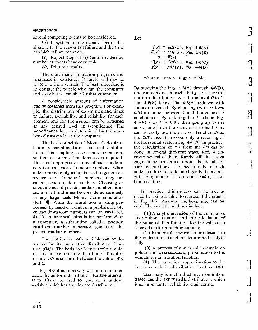
AMCP 706-196

several competing events to be considered. (6) If system failure occurs, record this

along with the reason for failure and the time at which failure occurred,

(7) Repeat Steps (l)-(6)until the desired number of events have occurred-

(8) Print out results.

There are many simulation programs and languages in existence. It rarely will pay to write one from scratch. The best procedure is to contact the people who run the computer and see what is available for that computer.

A considerable amount of information can be obtained from this program. For example, the distribution of downtimes and times to failure, availability, and reliability for each element and for the system can be obtained to any desired level of s-confidence. The s-confidence level is determined by the number of runs made on the computer.

The basic principle of Monte Carlo simulation is sampling from statistical distributions. This sampling process must be random, so that a source of randomness is required. The most appropriate source of such randomness is a sequence of random numbers. When a deterministic algorithm is used to generate a sequence of "random" numbers, they are called pseudo-random numbers. Choosing an adequate set of pseudo-random numbers is an art in itself and must be considered seriously in any large scale Monte Carlo simulation (Ref. 4). When the simulation is being performed by hand calculation, a published table of pseudo-random numbers can be used (Ref. 4). For a large scale simulation performed on a computer, a subroutine called a pseudo random number generator generates the pseudo-random numbers.

The distribution of a variable can be described by its cumulative distribution function (Cdf). The basis for Monte Carlo simulation is the fact that the distribution function of any Cdf is uniform between the values of 0 and 1.

Fig- 4-5 illustrates why a random number frcm the uniform distribution (onthe interval 0 to l)can be used to generate a random variable which has any desired distribution.

Let

f{x) = pdf{x}, Fig. 4-6(A) F(x) = Cdf{x), Fig. 4-6(B)

y = F(x) G(y) = Cdf{y], Fig. 4-6(C) g(y) = Pdf{y}, Fig. 46(D)

where x = any random variable,

By studying the Figs. 4-5(A) through 4-5(D), one can convince himself that y does have the uniform distribution over the interval 0 to 1. Fig. 4-5(E) is just Fig. 4-5(A) redrawn with the axes reversed. By choosing (withuniform pdf) a number between 0 and 1, a value of F is obtained. By entering the f-axis in Fig. 4-5(E) (say F = 0.6), then going up to the curve, one finds the value of x to be 4. One can as easily use the survivor function Sf as the Cdf since it involves only a reversing of the horizontal scale in Fig. 4-5(E). In practice, the calculations of x's from the F's can be done in several different ways. Ref. 4 discusses several of them. Rarely will the design engineer be concerned about the details of such calculations. He needs only enough understanding to talk intelligently to a computer programmer or to use an existing simulation routine.

In practice, this process can be mechanized by using a table to represent the graphs in Fig. 4-5. Analytic methods also can be used. The analytic methods include:

(1) Analytic inversion of the cumulative distribution function and the calculation of the value of this function for the value of a selected uniform random variable

(2) Numerical inverse interpolation in the distribution function determined analytically

(3) A process of numerical inverse interpolation in a numerical approximation to the cumulative distribution function

(4) The numerical approximation to the inverse cumulative distribution function itself.

The analytic method of inversion is illustrated far the exponential distribution, which is so important in reliability engineering.

3

] 3

J

4-10

A

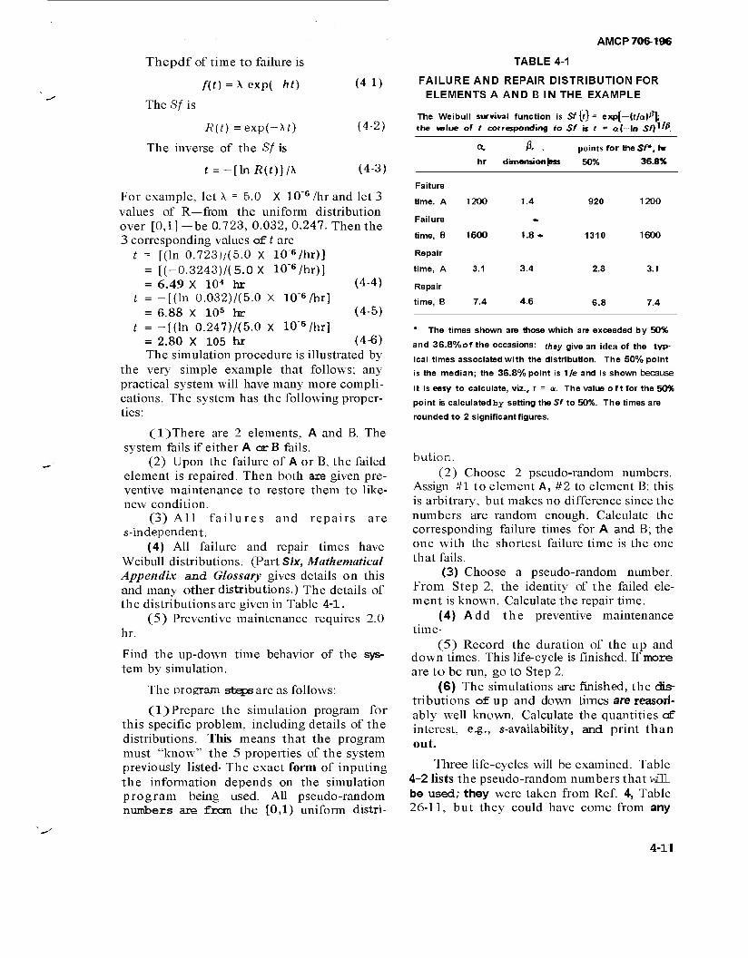
AMCP 706-196

Thepdf of time to failure is

f(t) =\ exp{~ht) (4-1)

The Sf is

R(t) =exp(-Af) (4-2)

The inverse of the Sf is

f = -[lnfi(0]A (43>

For example, let X = 5.0 X 10"6 /hr and let 3 values of R— from the uniform distribution over [0,1] -be 0.723, 0.032, 0.247. Then the 3 corresponding values of t are

t = [(In 0.7231/(5.0 X 10 6/hr)] = t(-0.3243)/(5.0X 10"6/hr)] = 6.49 X 10* hr (4-4)

t = -[(In 0.032)/(5.0 X lO^/hr) = 6.88 X 105 hr (4-5)

t = -[(In 0.247)/(5.0 X 10"6/hr] = 2.80 X 105 hr (4-6) The simulation procedure is illustrated by

the very simple example that follows; any practical system will have many more compli- cations. The system has the following properties:

(l)There are 2 elements, A and B. The system fails if either A or B fails.

(2) Upon the failure of A or B, the failed element is repaired. Then both are given preventive maintenance to restore them to like- new condition.

(3) All failures and repairs are «-independent.

(4) All failure and repair times have Weibull distributions. (Part Six, Mathematical Appendix and Glossary gives details on this and many other distributions.) The details of the distributions are given in Table 4-1.

(5) Preventive maintenance requires 2.0 hr.

Find the up-down time behavior of the system by simulation.

The program stgasare as follows:

(1) Prepare the simulation program for this specific problem, including details of the distributions. This means that the program must "know" the 5 properties of the system previously listed- The exact form of inputing the information depends on the simulation program being used. All pseudo-random numbers are from the [0,1) uniform distri-

TABLE 4-1

FAILURE AND REPAIR DISTRIBUTION FOR ELEMENTS A AND B IN THE EXAMPLE

The Weibull survival function Is Sf{f}= exp[—iffatfy the value of I corresponding to Sf is f = <*(—In SO "&.

a. A . points for the Sf*, hr

hr dimension |ess 50% 36.3%

Falture

time. A 1200 1.4 920 1200

Failure - time, B 1600 1.8 - 1310 1600

Repair

time, A 3.1 3.4 2.8 3.1

Repair

time, B 7.4 4.6 6.8 7.4

* The times shown are those which are exceeded by 50%

and 36.8%of the occasions: they give an idea of the typ-

ical times associated with the distribution. The 50% point

is the median; the 36.8% point is 1/e and is shown because

it is easy to calculate, viz., t = a. The value oft for the 50%

point Is calculated by setting theSf to 50%. The times are

rounded to 2 significant figures.

bution. (2) Choose 2 pseudo-random numbers.

Assign #1 to element A, #2 to element B: this is arbitrary, but makes no difference since the numbers are random enough. Calculate the corresponding failure times for A and B; the one with the shortest failure time is the one that fails.

(3) Choose a pseudo-random number. From Step 2, the identity of the failed element is known. Calculate the repair time.

(4) Add the preventive maintenance time-

(5) Record the duration of the up and down times. This life-cycle is finished. If more are to be run, go to Step 2.

(6) The simulations are finished, the distributions of up and down times are reasonably well known. Calculate the quantities of interest, e.g., »-availability, and print than out.

Three life-cycles will be examined. Table 4-2 lists the pseudo-random numbers that vül be used; they were taken from Ref. 4, Table 26-11, but they could have come from any

4-11

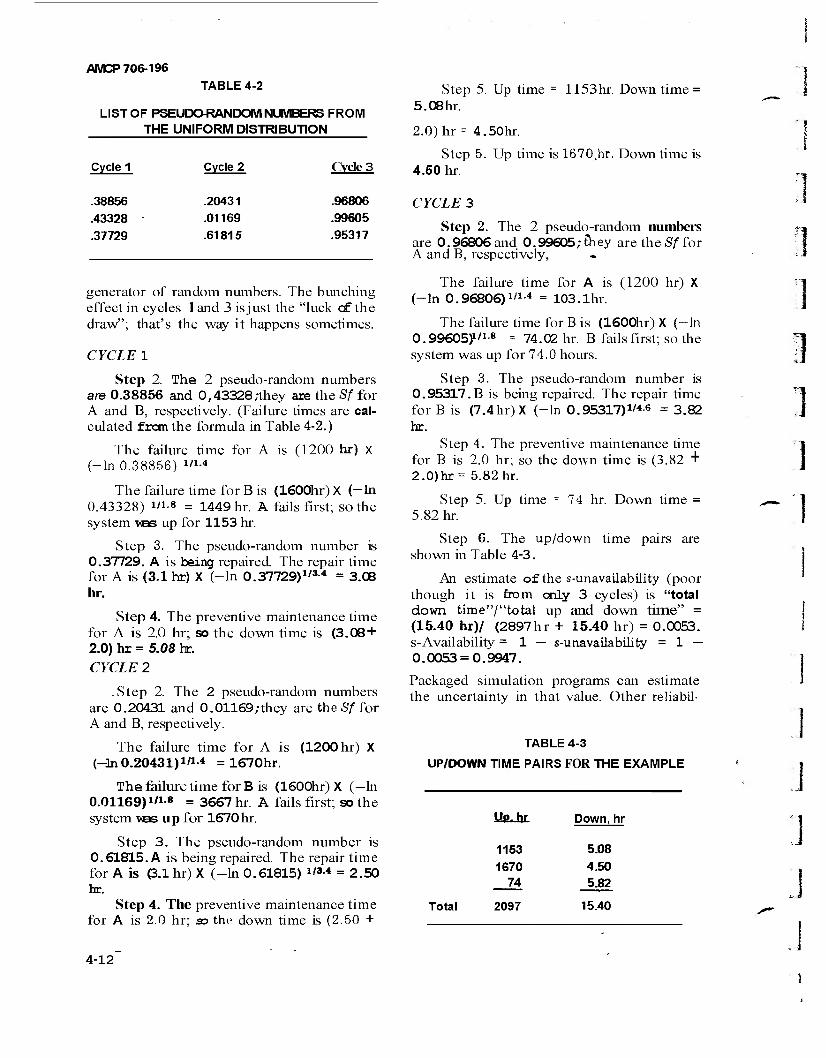
AMCP 706-196

TABLE 4-2

LIST OF PSEUDORANDOM NUMBERS FROM THE UNIFORM DISTRIBUTION

Cycle 1 Cycle 2 Cycle 3

Step 5. Up time = 1153hr. Down time = 5.08hr.

2.0) hr = 4.50hr.

Step 5. Up time is 1670,hr. Downtime is 4.50 hr.

.38856

.43328

.37729

.20431

.01169

.61815

.96806

.99605

.95317

generator of random numbers. The bunching effect in cycles land 3 is just the "luck cfthe draw"; that's the way it happens sometimes.

CYCLE 1

Step 2. The 2 pseudo-random numbers are 0.38856 and 0,43328,-they are the Sf for A and B, respectively. (Failure times are calculated from the formula in Table 4-2.)

The failure time for A is (1200 hr) X (-In 0.38856) »i-«

The failure time for B is (1600hr) X (-In 0.43328) i'1-8 = 1449 hr. A fails first; so the system vas up for 1153 hr.

Step 3. The pseudo-random number is 0.37729. A is being repaired. The repair time for A is (3.1 hr) X (-In 0.37729)1'3-4 = 3.08 hr.

Step 4. The preventive maintenance time for A is 2.0 hr; so the down time is (3.08 + 2.0) hr = 5.08 hr.

CYCLE 2

. Step 2. The 2 pseudo-random numbers are 0.20431 and 0.01169;they are the Sf for A and B, respectively.

The failure time for A is (1200 hr) X (-On 0.20431 )>/»•* = 1670hr.

The failure time for B is (1600hr) X (—In 0.01169)i'1-8 = 3667 hr. A fails first; so the system \««as up for 1670hr.

Step 3. The pseudo-random number is 0.61815. A is being repaired. The repair time for A is (3.1 hr) X (-In 0.61815) *'»-* = 2.50 hr.

Step 4. The preventive maintenance time for A is 2.0 hr; so the down time is (2.50 +

CYCLE 3

Step 2. The 2 pseudo-random numbers are 0.96806 and 0.99605,-they are the Sf for A and B, respectively,

The failure time for A is (1200 hr) X (-In 0.96806)1'1-4 = 103.Ihr.

The failure time for B is (1600hr) X (—In 0.99605p'18 = 74.02 hr. B fails first; so the system was up for 74.0 hours.

Step 3. The pseudo-random number is 0.95317.B is being repaired. The repair time for B is (7.4hr)X (-In 0.95317)1'4-6 = 3.82 hr.

Step 4. The preventive maintenance time for B is 2.0 hr; so the down time is (3.82 T

2.0)hr= 5.82 hr.

Step 5. Up time = 74 hr. Down time = 5.82 hr.

Step 6. The up/down time pairs are shown in Table 4-3.

An estimate of the s-unavailability (poor though it is from only 3 cycles) is "total down time"/"total up and down time" = (15.40 hr)/ (2897hr + 15.40 hr) = 0.0053. s-Availability = 1 — s-unavailability = 1 — 0.0053 = 0.9947.

Packaged simulation programs can estimate the uncertainty in that value. Other reliabil-

TABLE 4-3

UP/DOWN TIME PAIRS FOR THE EXAMPLE

Up.hr

1153 1870

74

Total 2097

Down, hr

5.08 4.50 5.82

15.40

4-12

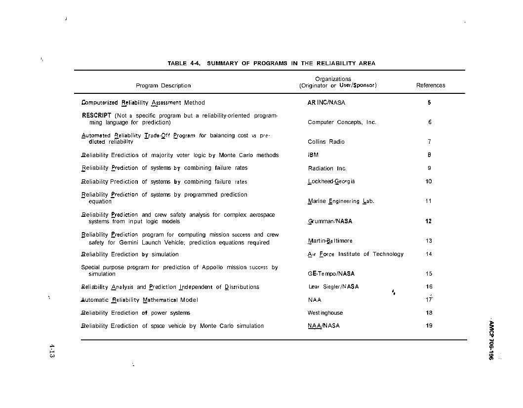
TABLE 4-4. SUMMARY OF PROGRAMS IN THE RELIABILITY AREA

Program Description Organizations

(Originator or User /Sponsor) References

Computerized Reliability Assessment Method

RESCRIPT (Not a specific program but a reliability-oriented programming language for prediction)

Automated Reliability £rade-Qff Program for balancing cost vs predicted reliability

.Reliability Erediction of majority voter logic by Monte Carlo methods

Reliability .Prediction of systems by combining failure rates

.Reliability Prediction of systems by combining failure rates

Reliability Prediction of systems by programmed prediction equation

.Reliability Prediction and crew safety analysis for complex aerospace systems from input logic models

.Reliability Prediction program for computing mission success and crew safety for Gemini Launch Vehicle; prediction equations required

.Reliability Erediction by simulation

Special purpose program for prediction of Appollo mission success by simulation

.Reliability .Analysis and .Prediction independent of Distributions

Automatic ^Reliability Mathematical Model

.Reliability Erediction of power systems

.Reliability Erediction of space vehicle by Monte Carlo simulation

AR INC/NASA 5

Computer Concepts, Inc. 6

Collins Radio 7

IBM 8

Radiation Inc. 9

Lockheed-Georgia 10

Marine .Engineering Lab. 11

Grumman/NASA 12

Martin-galtimore 13

Air Force Institute of Technology 14

GE-Tempo/NASA 15

Lear Siegler/NASA 16

NAA 17"

Westinghouse 18

NAA/NASA 19

t

W

9 o

£

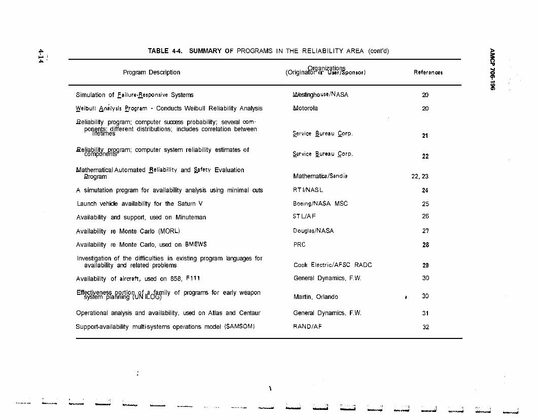
t TABLE 4-4. SUMMARY OF PROGRAMS IN THE RELIABILITY AREA (cont'd)

Program Description ,_ . . Organizations (Onginatora- Tfser/sponsor

Simulation of failure-jjjesponsive Systems

Welbull Analysis Program • Conducts Weibull Reliability Analysis

.Reliability program; computer success probability; several corn- its; difl times

nents; different distributions; includes correlation between iTetim

.Reliability program; computer system reliability estimates of components3 r ' '

Mathematical Automated Reliability and Safety Evaluation Erogram

A simulation program for availability analysis using minimal cuts

Launch vehicle availability for the Saturn V

Availability and support, used on Minuteman

Availability re Monte Carlo (MORD

Availability re Monte Carlo, used on BMEWS

Investigation of the difficulties in existing program languages for availability and related problems

Availability of aircraft, used on 858, F111

Effectiveness portion of aJamily of programs for early weapon

Operational analysis and availability, used on Atlas and Centaur

Support-availability multi-systems operations model (SAMSOM)

iufestingho use/NASA

.Motorola

Service Bureau Corp.

Service Bureau Corp,

Martin, Orlando

General Dynamics, F.W.

RAND/AF

References

20

20

21

22

Mathematica/Sandia 22,23

RTI/NASL 24

Boeing/NASA MSC 25

STL/AF 26

Douglas/NASA 27

PRC 28

Cook Electric/AFSC RADC 29

General Dynamics, I :.W. 30

30

31

32

> 3 o "V -4 O 9 i

Wtt*MwavK»i

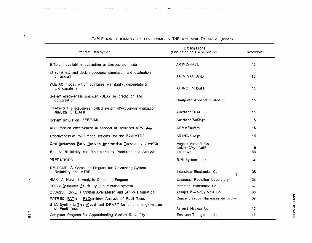
TABLE 4-4. SUMMARY OF PROGRAMS IN THE RELIABILITY AREA (cont'd)

Program Dercription Organirations

(Originator or User/Sponsor) References

en

Efficient availability evaluation as changes are made

Effectiveness and design adequacy simulation and evaluation of aircraft

WSEIAC model, which combines availability, dependability, and capability

System effectiveness analyzer (SEA) for prediction and optiraLtation

Steady-state effectiveness, called system effectiveness evaluation analyzer (SEE/AN)

System simulation (SEE/SIM)

ASW mission effectiveness in support of advanced ASW ship

Effectiveness of multi-mode systems, for the E2A/ATDS

Cost Reduction Early ßecision information Techniques (Oct73)

Routine Reliability and Maintainability Prediction and Analysis

PREDICTORS

RELCOMP: A Computer Program for Calculating System Reliability and MTBF

BIAS: A Network Analysis Computer Program

CROS: Computer Reliability optimization system

OLSASS: ^n-J_ine System Availability and Service simulation

PATREC: PATtern RECoonition Analysis of Fault Trees

STM: Synthetic Jree Model and DRAFT for automatic generation of Fault Trees

Computer Program for Approximating System Reliability

ARINC/NASL

ARINC/AF ASD

ARINC In-House

Computer Applications/NASL

Auerbach/DCA

Auerbach/BuShips

ARMA/BuWps

ARINC/BuWps

Hughes Aircraft Co. Culver City, Calif, unknown

R/M Systems, Inc.

Interstate Electronics Co. /

Lawrence Radiation Laboratory

Hoffman Electronics Co.

Aerojet ElectroSystems Co.

Centre d'Etude Nucleaires de Saclay

Aerojet Nuclear Co.

Research Triangle Institute

15

15

15

15

15

15

15

15

15 33

34

35

36

37

38

39

40

41

>

I

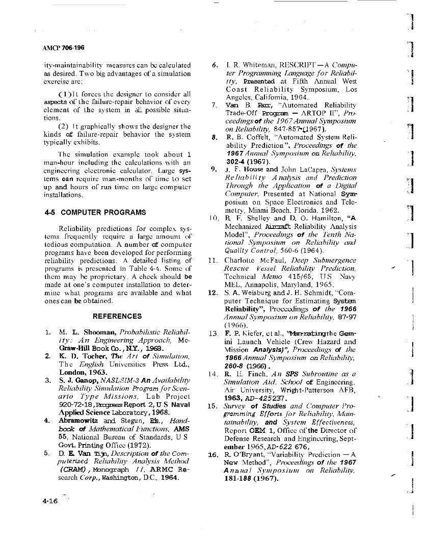
AMCP 706-196

ity-maintainability measures can be calculated as desired. Two big advantages of a simulation exercise are:

(l)It forces the designer to consider all aspects of the failure-repair behavior of every element of the system in all possible situations.

(2) It graphically shows the designer the kinds of failure-repair behavior the system typically exhibits.

The simulation example took about 1 man-hour including the calculations with an engineering electronic calculator. Large systems can require man-months of time to set up and hours of run time on large computer installations.

4-5 COMPUTER PROGRAMS

Reliability predictions for complex systems frequently require a large amount of tedious computation. A number of computer programs have been developed for performing reliability predictions. A detailed listing of programs is presented in Table 4-4. Some of them may be proprietary. A check should be made at one's computer installation to determine what programs are available and what ones can be obtained.

REFERENCES

1. M. L. Shooman, Probabilistic Reliabil- ity: An Engineering Approach, Mc- Graw-Hill Book Co., N.Y., 1968.

2. K. D. Tocher, The Art of Simulation, The English Universities Press Ltd., London, 1963.

3. S. J. Ganop, NASLSIM-3 An Availability Reliability Simulation Program for Scen- ario Type Missions, Lab Project 920-72-18,Progress Report 2,U S Naval Applied Science Laboratory, 1968.

4. Abramowitz and Stegun, Efe., Hand- bock of Mathematical Functions, AMS 55. National Bureau of Standards, U S Govt. Printing Office (1972).

5. D. E. Van TLjn, Description of the Com- puterized Reliability Analysis Method

(CRAM) , Monograph 11, ARMC Re- search Corp., Washington, D.C., 1964.

6. I. R. Whiteman, RESCRIPT -A Compu- ter Programming Language for Reliabil- ity, Presented at Fifth Annual West Coast Reliability Symposium, Los Angeles, California, 1964.

7. Van B. Barr, "Automated Reliability Trade-Off Program - ARTOP II", Pro- ceedings of the 1967 Annual Symposium on Reliability, 847-857-11967).

8. R. B. Coffelt, "Automated System Reli- ability Prediction", Proceedings of the 1967Annual Symposium on Reliability, 302-4(1967).

9. j. F. House and John LaCapra, Systems Re Habili ty A nalysis and Prediction Through the Application of a Digital Computer, Presented at National Sym- posium on Space Electronics and Tele- metry, Miami Beach, Florida, 1962.

10. B. F. Shelley and D. O. Hamilton, "A Mechanized Aircraft Reliability Analysis Model", Proceedings of the Tenth Na- tional Symposium on Reliability and Quality Control, 560-6 (1964).

11. Charlotte McFaul, Deep Submergence Rescue Vessel Reliability Prediction, Technical Memo 415/65, US Navy MEL, Annapolis, Maryland, 1965.

12. S. A. Weisburg and J. H. Schmidt, "Com- puter Technique for Estimating System Reliability", Proceedings of the 1966 Annual Symposium on Reliability, 87-97 (1966).

13. F. P. Kiefer, etal., "Ixbn-ratingthe Gem- ini Launch Vehicle (Crew Hazard and Mission Analysis)", Proceedings of the 1966 Annual Symposium on Reliability, 260-8 (1966).

14. R. E. Finch, An SPS Subroutine as a Simulation Aid, School of Engineering, Air University, Wright-Patterson AFB, 1963, AD-425231.

15. Survey of Studies and Computer Pro- gramming Efforts for Reliability, Main- tainability, and System Effectiveness, Report OEM 1, Office of the Director of Defense Research and Engineering, Sept- ember 1965,AD-622 676,

16. R. O'Bryant, "Variability Prediction —A New Method", Proceedings of the 1967 Annual Symposium on Reliability, 181-188 (1967).

1 1 1

4-16

AMCP 706-196

17. C. W. McKnight, et al., "An Automatic Reliability Mathematical Model", Pro- ceedings of the Eleventh National Symposium on Reliability and Quality Control, 518-32 (1965).

18. A. D. Patton, et ah, "Power System Reli- ability II —Applications and a Computer Program", IEEE Transactions on Power Apparatus and Systems PAS-84, 636 (July 1965).

19. B. H. Hershkowitz, et al., "Reliability Simulation Model", Proceedings of the Tenth National Symposium on Reliabil- ity and Quality Control, 186-200 (1964).

20. J. M. Hannigan, A Computer Program for the Simulation of Failure-Responsive Systems, Technical Report No. 6, West- inghouse Defense and Space Center, 1966,N66-26880.

21. Reliability Engineering at SBC, Service Bureau Corporation, Computing Sci- ences Division, Palo Alto, California. 1066.

22. A Description of the MARSEP Program — A Mathematica Report, Mathematica, Inc., Princeton, N.J., July 1969.

23. A. M. Breipohl and R. A. Hemquist, A Computer Program for Performing Reli- ability Analyses, Report SC-TM-65-523, Sandia Laboratory, Albuquerque, New Mexico, December 1965.

24. Evaluation of Computer Programs for System Performance Effectiveness, Vol- ume II, RTI Project SU-285, Research Triangle Institute, Research Triangle Park, North Carolina 27709, August 1967.

25. "Computer Tells Launch Vehicle Readi- ness", Technology Week (April 1967).

26. J. Dresner and K. H. Borchers, "Mainte- nance, Maintainability and System @- quirements Engineering", Proceedings of the Third Annual Aerospace Reliability and Maintainability Conference (1964).

27. AM. Economos, "A Monte Carlo Simu- lation for Maintenance and Reliability", Proceedings of the Third Annual Aero- space Reliability and -Maintainability Conference (1964). - .

28. W. E. Faragher and H. S. Watson, "Avail- ability Analyses — A Realistic Method- ology' *, Proceedings of the Tenth Na-

tional Symposium on Reliability and Quality Control, 365-78 (1964).

29. T. J. Horrigan, Development of Tech- niques for Prediction of System Effec- tiveness, RADC TDR-63-407, Cook Elec- tric Company, February 1964, AD-432 844.

30. "Maintainability Trade-off Techniques", Maintainability Bulletin No. 8, Elec- tronic Industries-Association, July 1966.

31. R. K. Ruhe, "Logic Simulation for System Integration and Design Assur- ance", Proceedings of the Third Annual Aerospace Reliability and Maintain- ability Conference (1964).

32. T. C. Smith, "The Support-Availability Multi-System Operations Model", Pro- ceedings of the Third Annual Aerospace Reliability and Maintainability Confer- ence (1964) .

33. A. C. Spann, "A Synergistic Reliability and Maintainability Prediction Package", Proceedings of the 1973 Annual Zfeli- ability and Maintainability Symposium, 542-549 (1973).

34. K. G. Blemel, "Computer Software Synergism Integrates R/M Design", Pro- ceedings of the 1974 Annual Reliability and Maintainability Symposium, 68-72 (1974).

35. J. L. Fleming, "Relcomp: A Computer Program for Calculating System Reli- ability and MTBF", IEEE Trans. Reli- ability R-20, 102-107 (August 1971).

36. J. L. Willows and W. G. Magnuson, Jr., "Bias: A Network Analysis Computer Program Useful to the Reliability Engi- neer", IEEE Trans. Reliability R-20, 108-116 (August 1971).

37. A. S. Cici and V. O. Muglia, "Computer Reliability Optimization System", IEEE Trans. Reliability R-20, 110-116 (August , 1971).

38. Irving Doshay, "On-Line System Avail- ability and Service Simulation (OL- SASS)", IEEE Trans. Reliability R-20, 142-147 (August 1974).

39. B. V. Koen and A. Camino, "Reliability Calculations with a List Processing Tech- nique", IEEE Trans. Reliability R-23 (April 1974).

40. J. B. Fussell, Synthetic Tree Models: A Formal Methodology for Fault Tree

4-17

AMCP 706-196

Construction, ANCR-1098, UC-32, «A Computer Program far Approxi- 1 Aeroject Nuclear Cb., Idaho Falls, Idaho mating System Reliability", IEEE Trans. ) 83401,March 1973. Reliability R-19,61T£5 (May 1970) and

41. A C. Nelson, J. R. Batts, R. L. Beadles, R.20,88-90 (May 1971). _

1

v ]

4-18

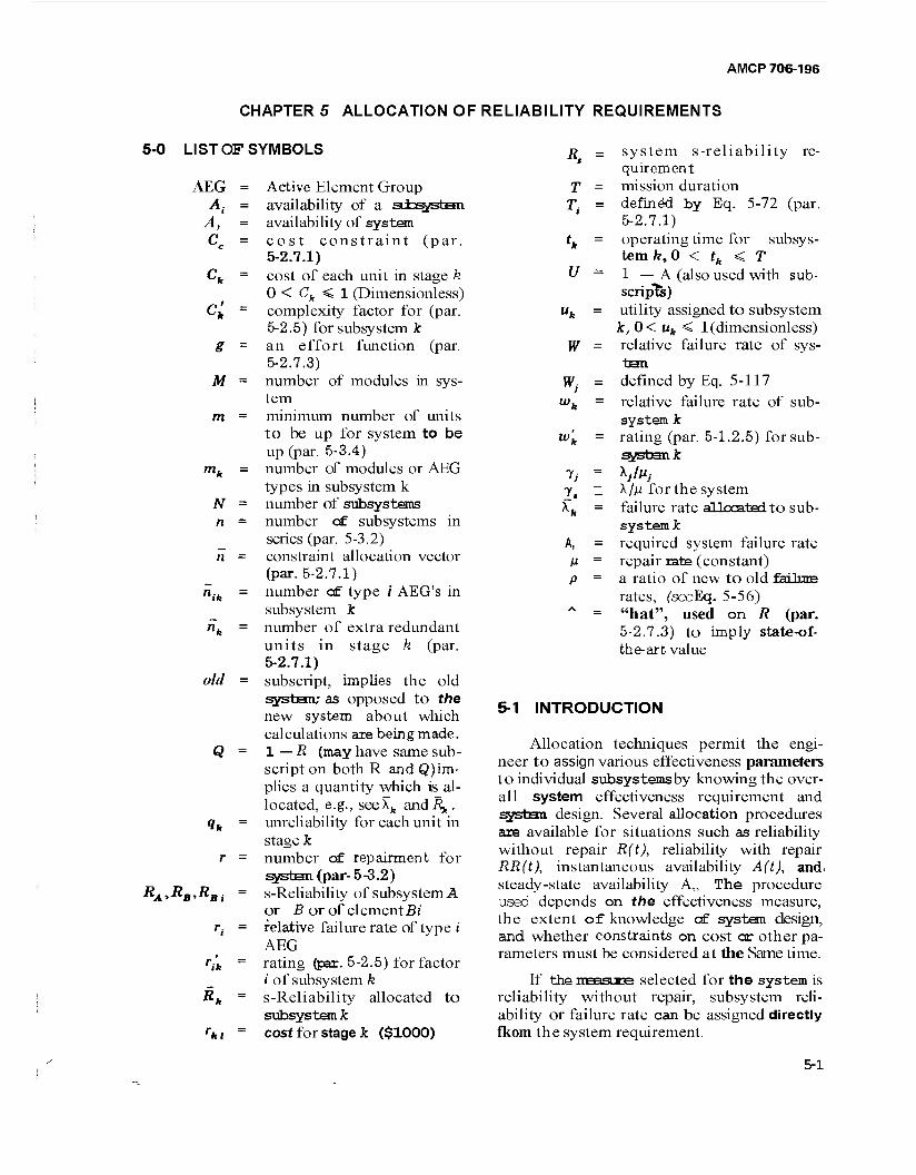
AMCP 706-196

CHAPTER 5 ALLOCATION OF RELIABILITY REQUIREMENTS

m =

mu =

5-0 LIST OF SYMBOLS

AEG = Active Element Group A( = availability of a subsystan

A, = availability of system Cc = cost constraint (par.

5-2.7.1) Ck = cost of each unit in stage k

0 < Ck < 1 (Dimensionless) Ck = complexity factor for (par.

5-2.5) for subsystem k g ~ an effort function (par.

5-2.7.3) M = number of modules in sys-

tem minimum number of units to be up for system to be up (par. 5-3.4) number of modules or AEG types in subsystem k

N - number of subsystems n - number cf subsystems in

series (par. 5-3.2) n = constraint allocation vector

(par. 5-2.7.1) number cf type / AEG's in subsystem k number of extra redundant units in stage k (par. 5-2.7.1)

old = subscript, implies the old systaii; as opposed to the new system about which calculations are being made.

Q = 1 — R (may have same subscript on both R and Q) implies a quantity which is allocated, e.g., seeXfe and J^ .

qk = unreliability for each unit in stage k

r = number of repairment for systen (par- 5-3.2) s-Reliability of subsystem A or B or of el ement Bi relative failure rate of type i AEG rating (par. 5-2.5) for factor i of subsystem k

Rk - s-Reliability allocated to subsystem k

rkl ~ cost for stage k ($1000)

lih

nh

RA>RB*RBi ~

r.

'ife

R = system s-reliability requirement

T = mission duration T. = defined by Eq. 5-72 (par.

5-2.7.1) rfc = operating time for subsys-

tem fe, 0 < tk < T U = 1 — A (also used with sub-

scripts) uh = utility assigned to subsystem

k, 0< uk < 1 (dimensionless) W = relative failure rate of sys-

tem Wj = defined by Eq. 5-117

wh = relative failure rate of subsystem k

w'k = rating (par. 5-1.2.5) forsub- sysban. k

yt - ^/M for the system Xfe = failure rate allocatEd to sub-

system k A, = required system failure rate

M = repair rate (constant) p = a ratio of new to old failure

rates, (seeEq. 5-56) A = "hat", used on R (par.

5-2.7.3) to imply state-of- the-art value

5-1 INTRODUCTION

Allocation techniques permit the engineer to assign various effectiveness parameters to individual subsystems by knowing the overall system effectiveness requirement and systBii design. Several allocation procedures are available for situations such as reliability without repair R(t), reliability with repair RR(t), instantaneous availability A(t), and- steady-state availability A„ The procedure used depends on the effectiveness measure, the extent of knowledge cf system design, and whether constraints on cost or other parameters must be considered at the Same time.

If the measure selected for the system is reliability without repair, subsystem reliability or failure rate can be assigned directly fkom the system requirement.

5-1

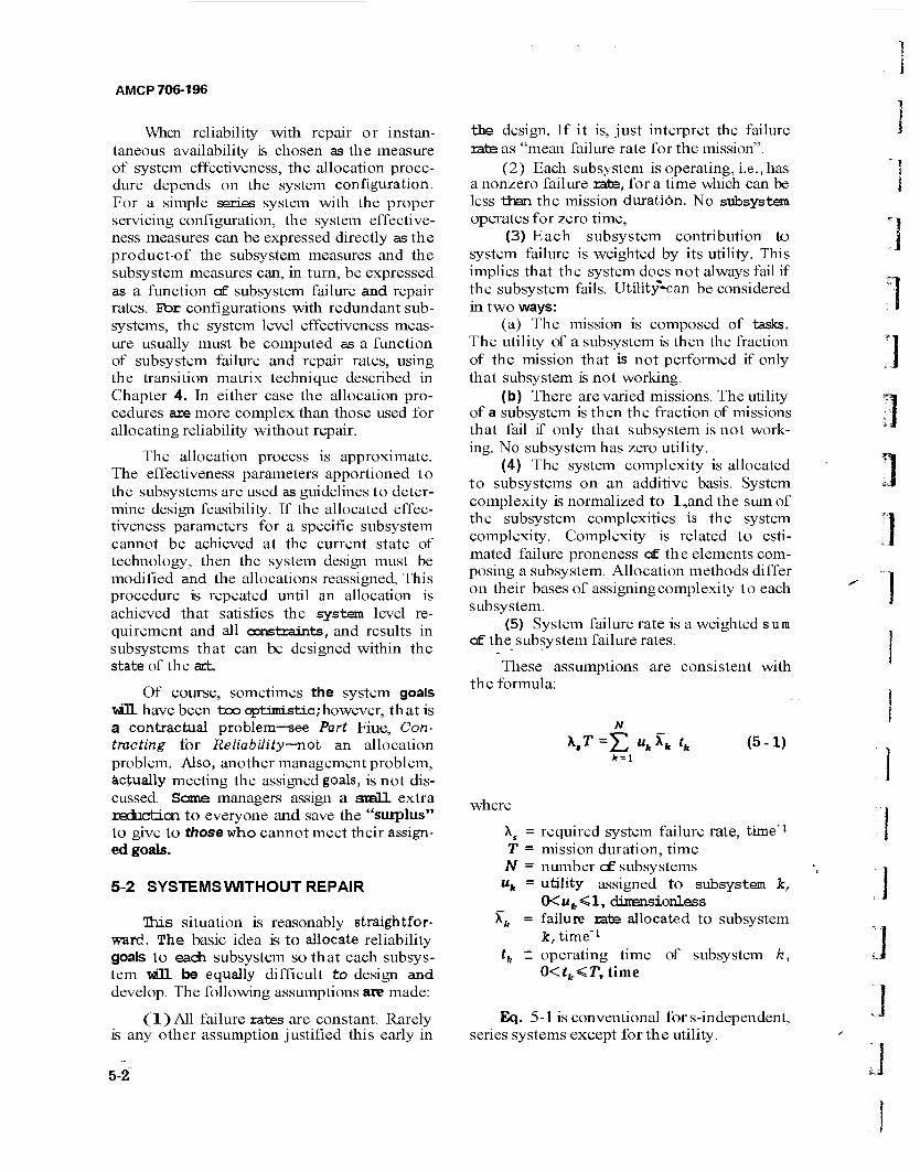
AMCP 706-196

When reliability with repair or instantaneous availability is chosen as the measure of system effectiveness, the allocation procedure depends on the system configuration. For a simple series system with the proper servicing configuration, the system effectiveness measures can be expressed directly as the product-of the subsystem measures and the subsystem measures can, in turn, be expressed as a function cf subsystem failure and repair rates. For configurations with redundant subsystems, the system level effectiveness measure usually must be computed as a function of subsystem failure and repair rates, using the transition matrix technique described in Chapter 4. In either case the allocation procedures are more complex than those used for allocating reliability without repair.

The allocation process is approximate. The effectiveness parameters apportioned to the subsystems are used as guidelines to determine design feasibility. If the allocated effectiveness parameters for a specific subsystem cannot be achieved at the current state of technology, then the system design must be modified and the allocations reassigned, This procedure is repeated until an allocation is achieved that satisfies the system level requirement and all constraints, and results in subsystems that can be designed within the state of the art.

Of course, sometimes the system goals wüß. have been too optimistic;however, that is a contractual problem—see Part Fiue, Con- tracting fbr ReliabÜity—not an allocation problem. Also, another management problem, actually meeting the assigned goals, is not discussed. Some managers assign a grail extra reduction to everyone and save the "surplus" to give to those who cannot meet their assigned goals.

5-2 SYSTEMS WITHOUT REPAIR

This situation is reasonably straightforward. The basic idea is to allocate reliability goals to each subsystem so that each subsystem VÜL be equally difficult to design and develop. The following assumptions are made:

(1)A11 failure rates are constant. Rarely is any other assumption justified this early in

the design. If it is, just interpret the failure rate as "mean failure rate for the mission".

(2) Each subsystem is operating, i.e., has a nonzero failure rate, for a time which can be less than the mission duration. No subsystem operates for zero time,

(3) Each subsystem contribution to system failure is weighted by its utility. This implies that the system does not always fail if the subsystem fails. Utility~can be considered in two ways:

(a) The mission is composed of tasks. The utility of a subsystem is then the fraction of the mission that is not performed if only that subsystem is not working.

(b) There are varied missions. The utility of a subsystem is then the fraction of missions that fail if only that subsystem is not working. No subsystem has zero utility.

(4) The system complexity is allocated to subsystems on an additive basis. System complexity is normalized to l,and the sum of the subsystem complexities is the system complexity. Complexity is related to estimated failure proneness cf the elements com- posing a subsystem. Allocation methods differ on their bases of assigning complexity to each subsystem.

(5) System failure rate is a weighted sum cf the subsystem failure rates.

These assumptions are consistent with the formula:

N X.T=£ ukKtk (5-1)

h-1

where

\t = required system failure rate, time*1

T = mission duration, time N = number cf subsystems uh = utility assigned to subsystem k,

(X«fc<l, dimensionless \b = failure rate allocated to subsystem

k, time"1

th - operating time of subsystem k, 0<afe«7\time

Eq. 5-1 is conventional for s-independent, series systems except for the utility.

5-2

AMCP 706-196

The following allocation cf failure rate is consistent with Eq. 5-1.

X. = Vfe (tkIT)uk \ (5-2)

where

Ck = complexity factor of subsystem k, N

0 < Ck < l»2jCk = 1, dimensionless

If Xfc in Eq. 5-2 is substituted in Eq. 5-1, an identity results, which demonstrates that Eq. 5-2 is indeed a solution to Eq. 5-1.

5-2.1 EQUAL ALLOCATION

This is the simplest situation. It arises under the following additional assumptions about the system:

(1) JQ1 utilities are 1: uk = lfor all k (2) 2Ü1 subsystems operate for the entire

mission: tk = Tfor all k (3) Each subsystem is of equal com-

plexity: Ck = 1/WforaU k.

Eq. 5-2 becomes

X, =(l/iV)X,. (5-3)

Eq. 5-3 is equivalent to

Sk=R,^ (5-4)

where

Rk = s-Reliability allocated to each subsystem

JRS = systems-reliability requirement

When the s-reliability R is near 1, it is often desirable to calculate the s-unreliability Q.

Q=l- R (5-5)

It is easier to understand, because it is the probability of failure. Example Problem No. 1 illustrates the application cf reliability goals.

5-22 PROPORTIONAL COMPLEXITY

When a new system is very similar to an

old one, with the exception of a new reliability requirement, Eq. 5-2 can be simplified. The basic assumption is that

Ck \,old (tJT)uk \,old

(5-8)

where

old = subscript denoting the old system.

Eq. 5-2, when combined with Eq. 5-8, simplifies to

*fe ~ ^k.o 'a X s.old (5-9)

Example Problem No. 2 illustrates the procedure.

5-2.3 SIMPLE-MODULAR COMPLEXITY

Each subsystem is presumed to be composed of s-independent modules in series, each of which has the Same failure rate. Com- plexity is taken to be the fraction of modules - in the subsystem

Ck=mJM (5-15)

where tnk = number of modules in subsystem k M = number of modules in the system

Then Eq. 5-2 becomes

_ (mk/M) k ' (tJT)uk

A« (5-16)

Example Problem No. 3 illustrates the procedure.

It is possible to calculate subsystem s-reliab$- ity, but its meaning is distorted by the utility and operating time factors in Eq. 5-1. It is better not to make the calculation since the proper explanations will be lost too easily, and the results will appear erroneous without the explanations.

5-3

AMCP 706-196

Example Problem No. 1

A group of 8 roller bearings is required to have an s-reliability of 0.99 and the conditions of Eqs. 5-3 and 5-4 are assumed to be satisfied. What s-reliability is to be allocated to each bearing?

Procedure

(1) Set Rs to the required system s-reliability, and N to the number of subsystems. Solve also for Q, by Eq. 5-5.

Example

RM = 0.99 N=8

Q, = 1-0.99=0.01 (5-6)

(2) Solve for Rh by Eq. 5-4 and Qk by Eq. 5-5.

Rh =(0.99) »'8=0.99874 Qk = 1 - 0.99874 = 0.00126

(5-7)

Each bearing can have only about 1/8 the failure probability of the whole system. The application cf the formulas presumes that bearing failures are s-independent of each other; e.g., failure is not due to a sudden stoppage of lubrieating-oil flow to all bearings.

5^1

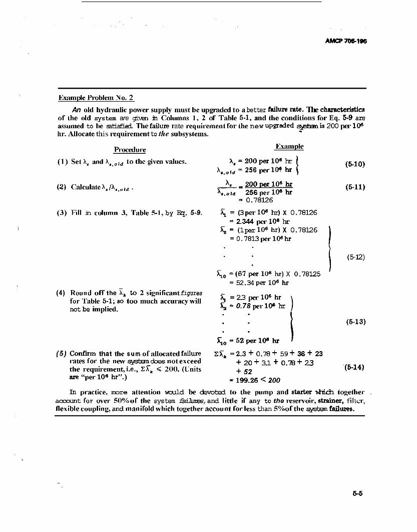
AMCP 706-196


An old hydraulic power supply must be upgraded to a better failure rate. The characteristic« of the old system are given in Columns 1, 2 of Table 5-1, and the conditions for Eq. 5-9 are assumed to be satisfied. The failure rate requirement for the new upgraded j^stanis 200 per 106

hr. Allocate this requirement to the subsystems.

Procedure

(1) Set X5 and X, old to the given values.

(2) CalculateX,/X,j0ld .

(3) Fill ±i column 3, Table 5-1, by Eq. 5-9.

Example

X# = 200 per 10« hr j ,ld = 256 per 10« hr j 256 per:

200 per 10« hr __A-„ - K.otd 256 per 10« hr

= 0.78126

\ = (3per 10« hr) X 0.78126 » 2.344 per 10« hr

X^ = (lper 10« hr) X 0.78126 = 0.7813 per 10« hr

(5-10)

(5-11)

(4) Round off the \k to 2 significant figures for Table 5-1; so too much accuracy will not be implied.

(5) Confirm that the sumof allocated failure rates for the new ^standees not exceed the requirement, i.e., ZXk < 200. (Units are "per 10« hr".)

\o

(5-12)

= (67 per 10« hx) X 0, = 52.34 per 10« hr

78125

= 23 per 10« hr " 0.78 per 10« hr )

(5-13)

X^0 - 52 per 10« hr

ZX* = 2.3 + 0.78 +59+36+23 + 20 + 3.1 + 0.78 + 23 + 52

= 199.26 < 200

(5-14)

In practice, more attention would be devoted to the pump and starter vhkri together account for over 50% of the system iäüzzss, and little if any to the reservoir, strainer, filter, flexible coupling, and manifold which together account for less than 5%of the system failures.

5-5

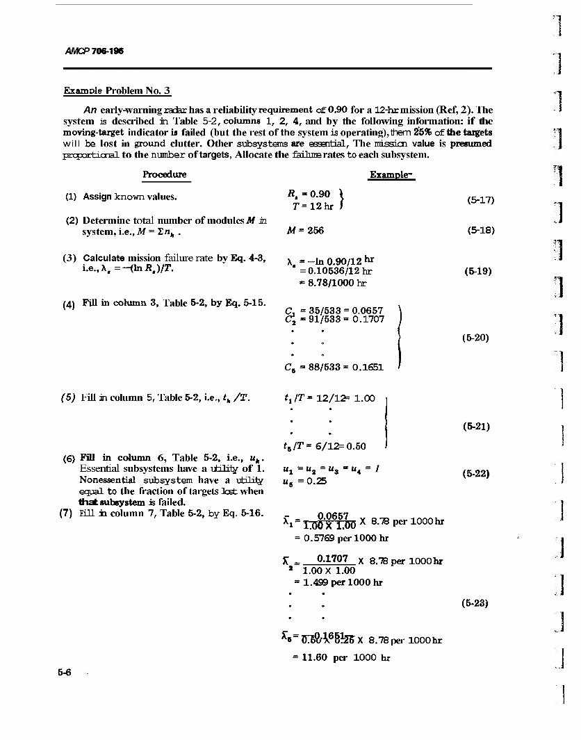
AMCP 706-196


An early-warning radar has a reliability requirement of 0.90 for a 12-hr mission (Ref, 2). The system is described in Table 5-2, columns 1, 2, 4, and by the following information: if the moving-target indicator is failed (but the rest of the system is operating), them 25% of the targets will be lost in ground clutter. Other subsystems are essential, The irdssicn value is presumed proportional to the number of targets, Allocate the failure rates to each subsystem.

Procedure

(1) Assign known values.

(2) Determine total number of modules M in system, i.e., M = *Lnh .

(3) Calculate mission failure rate by Eq. 4-3, i.e.,X, =-(ln R.)fT.

(4) Fill in column 3, Table 5-2, by Eq. 5-15.

Example"

R, = 0.90 \ r=12hr /

Jlf = 256

X. = -In 0.90/12 *"" = 0.10536/12 hr = 8.78/1000 hr

C, =35/533 = 0.0657 C\ =91/533 = 0.1707

C6 = 88/533= 0.1651

(5-17)

(5-18)

(5-19)

(5-20)

(5) Fill in column 5, Table 5-2, i.e., th /T.

(6) Fill in column 6, Table 5-2, i.e., uk. Essential subsystems have a utility of 1. Nonessential subsystem have a utility equal to the fraction of targets lest when that subsystem is failed.

(7) Fill ±1 column 7, Table 5-2, by Eq. 5-16.

fj/r- 12/12= 1.00

th/T= 6/12=0.50

"x Ä "a = "s = u4 = 1 u6 =0.25

Xi = I^XrJüX 8.78 per 1000 hr = 0.5769 per 1000 hr

% m 0.1707 x 8.78 per 1000hr 2 1.00 X 1.00

= 1.499 per 1000 hr

*»~ TT&jlPhhE X 8.78per 1000hr

= 11.60 per 1000 hr

(5-21)

(5-22)

(5-23)

5-6

AMCP 706-196

(8) Round off Xft to 2 significant figures for Table 5-2, column 7; so too much accuracy will not be implied.

The failure rates ±i column 7, Table 5-2 do not sum to X, = 8.78 per 1000 hr (Eq. 5-19) because of the various weighting factors. To check the calculations, Eq. 5-1 has to be used.

(9) Fill in column 8, Table 5-2, i.e., uk\kth.

X, =0.58 per 1000 hr.

X5 = 12 per 1000hr

(5-24)

1)1.00X (0.58/1000 hr)X 12 hr = 0.00696

(5-25)

(10) Sum column 8 by Eq. 5-1.

5) 0.25X (12/1000 hr)X 6 hr = 0.01800

S = 0.00696 + 0.01800+ 0.1680 + 0.04560 + 0.01800

= 0.1054

(11) Compare with requirement XfT = 8.78 X Q 1054 < 0 1054 12 = 0.1054

(5-26)

(5-27)

The requirement is satisfied to within the accuracy of the problem statement.

5-7

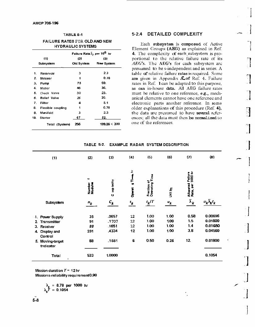
AMCP 706-196

TABLE 5-1

FAILURE RATES FOR OLD AND NEW HYDRAULIC SYSTEMS

Failure Rate A,-, per 106 hr

(1) 12) (3)

Subsystem Old System N BW System

1. Reservoir 3 2.3

2. Strainer 1 0.78

3. Pump 75 59.

4. Motor 46 36.

5. Check Valve 30 23.

6. Relief Valve 26 20.

7. Filter 4 3.1

8. Flexible coupling 1 0.78

9. Manifold 3 2.3

10. Starter

Total (System)

67 52.

256 199.26 < 200

5-2.4 DETAILED COMPLEXITY

Each subsystem is composed of Active Element Groups (AEG) as explained in Ref. 4. The complexity of each subsystem is proportional to the relative failure rate of its AEG's. The AEG's for each subsystem are presumed to be s-independent and in series. A table of relative failure rates is required. Some are given in Appendix ÄLof Ref. 4. Failure rates in Ref. lean be adapted to this purpose, as can in-house data. All AEG failure rates must be relative to one reference, e.g., mechanical elements cannot have one reference and electronic parts another reference. In some older explanations of this procedure (Ref. 4), the data are presumed to have several references; all the data must then be normalized to one of the references.

] TABLE 5-2. EXAMPLE RADAR SYSTEM DESCRIPTION

<1) (2) (3) (4) (5) (6) (7) (8) - \

> "5 .• a E o

I-

•* •

o o c c OS

Si. u-O

E

5

• •

Subsystem nk ck fk V uk ** ukhfk

1. Power Supply 35 .0657 12 1.00 1.00 0.58 0.00696

2. Transmitter 91 .1707 12 1.00 1.00 1.5 0.01800

3. Receiver 88 .1651 12 1.00 1.00 1.4 0.01680

4. Display and 231 .4334 12 1.00 1.00 3.8 0.04560

Control 5. Moving-target 88 .1651 6 0.50 0.25 12. 0.01800

tndicator

Total 533 1.0000 0.1054

Mission duration T- 12 hr Missions-reliability requirement0.90

>5 = 8.78 per 1000 hr \T = 0.1054

5-8

AMCP 706-196

The subsystem complexity is

Ck=wJW (5-28)

wk =y"r. nik (5-29) i= 1

W=Y,wk (5-30) k = I

where

r. = i

wk = W =

m^. =

number of type i AEG's in subsystem k relative failure rate of type i AEG relative failure rate of subsystem k relative failure rate of the system number of AEG types in subsystem k


5-2.5 FEASIBILITY-OF-OBJECTIVES AL- LOCATIONS

This technique adapted from Ref. 5 was developed primarily as a method of allocating reliability without repair, for mechanical- electrical systems. In this method, subsystem allocation factors are computed as a function of numerical ratings of system intricacy, state of the art, performance time, and environmental conditions. These ratings are estimated by the engineer on the basis of his experience. Each rating is on a scale from lto 10,with values assigned as discussed:

(1) System Intricacy, intricacy is evaluated by considering the probable number of parts or components making up the system and also is judged by the assembled intricacy cf these parts car components. The least intri- cate system is rated at 1, and a highly intri- cate system is rated at 10.

(2) State of the Art. The state cf present engineering progress in all fields is considered. The least developed design or method is assigned a value of 10, and the most highly developed is assigned a value of 1.

(3) Performance Time. The element that operates for the entire mission time is rated 10, and the element that operates the least time during the mission is rated at 1.

(4) Environment. Environmental conditions are also rated from 10 through 1. Ele- ments expected to experience harsh and very severe environments during their operation aiB rated as 10, and those expected to en- counter the least -severe environments are rated as 1.

The ratings are assigned by the engineer using his engineering know-how and experience. An estimate is made of the types of parts and components likely to be used in the new system and what effect their expected use has on their reliability. If particular components had proven to be unreliable in a particular environment, the environmental rating is raised- The ratings can be selected by individual engineers, or through some form of voting technique among a group of design engineers.

The 4 ratings for each subsystem are multiplied together to give a rating for the subsystem; the subsystem rating will be between 1 and 104. The subsystem ratings are then normalized so that their sum is 1. The normalized subsystem rating C'h is used in place of the factor C, l(tk/T) in Eq. 5-2. The utility of each subsystem is considered to be l.Eqs. 5-1 and 5-2then become

Vr=X>hT (5-42) k=l

K=C>\ (5-43]

where

C = complexity of subsystem k

C'^w'JW' (5-44) r

t t i t t Wk " rikr2k r3k r4fe (5-45)

N

wu (5-46) *=i

5-9

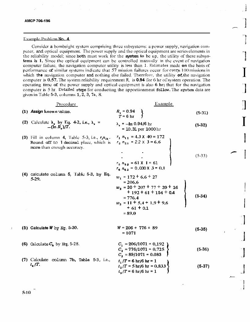
AMCP 706-196

Fvample Prnhlem Nn A

Consider a bombsight system comprising three subsystems: a power supply, navigation computer, and optical equipment. The power supply and the optical equipment are series elements in the reliability model; since both must work for the systsn to be up, the utility of these subsystems is 1. Since the optical equipment can be controlled manually in the event of navigation computer failure, the navigation computer utility is less than 1. Estimates made on the basis of performance of similar systems indicate that 57 mission failures occur for every. 100 missions in which the navigation computer and nothing else failed. Therefore, the utility of,the navigation computer is 0.57. The system reliability requirement R, is 0.94 for 6 hr of system operation. The operating time of the power supply and optical equipment is also 6 hr; that for the navigation computer is 5 hr. Detailed steps for conducting the apportionment follow. The system data are given in Table 5-3, columns 1,2, 3, 7a, 8.

Procedure

(1) Assign known valuss.

(2) Calculate X, by Eq. 4-2, i.e., X, = _(lnÄ,)/T.

(3) Fill in column 4, Table 5-3, i.e., r^^. Round off to 1 decimal place, which is more than enough accuracy.

(4) calculate column 5, Table 5-3, by Eq. 5-29.

Example

Rt = 0.94 T = 6hr

X, = -In 0.94/6 hr = 10.31 per 1000 hr

ri nti =4.3X 40= 172 r2 n21 = 2.2 X 3 = 6.6

r5 n53 =61 X 1= 61 r6 n63 = 0.030X 3= 0.1

(5-31)

(5-32)

(5-33)

w.

w.

w,

= 172+ 6.6 + 27 = 206.6 = 30 + 207 +77 + 39+16

+ 192 + 61 + 154 + 0.4 = 776.4 = 11 + 5.4+ 1.9+ 9.6

+ 61 + 0.1 = 89.0

(5-34)

I

]

I

(5) Calculate W by Eq. 5-30. W = 206 + 776 + 89 = 1071

(5-35)

(6) Calculate Ck by Eq. 5-28.

(7) Calculate column 7b, Table 5-3, i.e., tJT.

Ct =206/1071 = 0,192 C2 = 776/1071 = 0.725 C3 = 89/1071 = 0.083

t1/T = 6 hr/6 hr = 1

*2/r = 5hr/6hr=0.833 t3/7' = 6hr/6hr = l

(5-36)

(5-37)

5-10

s . ,1

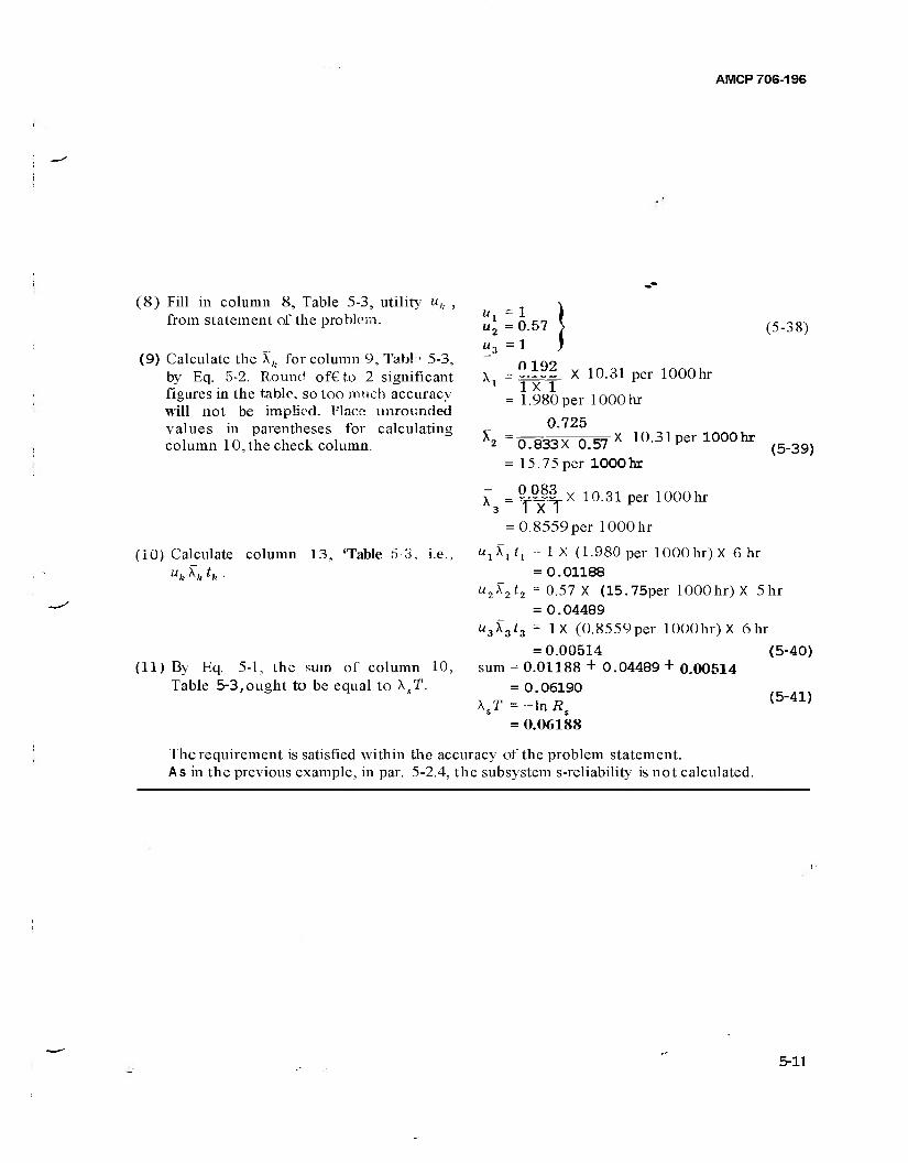
AMCP 706-196

(8) Fill in column 8, Table 5-3, utility ult , from statement of the problem.

(9) Calculate the %,. for column 9, Tabl ■ 5-3, by Eq. 5-2. Round of€to 2 significant figures in the table, so too much accuracy will not be implied. Place unrounded values in parentheses for calculating column 10, the check column.

(10) Calculate column 13, 'Table 6 3, i.e., ufe\*fc ■

(11) By Eq. 5-1, the sum of column 10, Table 5-3,ought to be equal to X,T.

u2 =0.57 \ u3=l )

x = ?.*?? x 10.31 per lOOOhr 1 TxT = 1.980 per lOOOhr

0.725 0T833X 0.57 X 10.31 per 1000hr

(5-38)

K =

= 15.75 per lOOOhr

0 083

(5-39)

X 10.31 per lOOOhr S'TTT = 0.8559per lOOOhr

utX, ty = 1 X (1.980 per lOOOhr) X 6 hr = 0.01188

u2\2t2 = 0.57 X (15.75per lOOOhr) X 5 hr = 0.04489

U3X3/3 = IX (0.8559per lOOOhr) X 6hr

= 0.00514 (5-40) sum = 0.01188 + 0.04489 + 0.00514

= 0.06190 XST =-lnÄ,

= 0.06188

(5-41)

The requirement is satisfied within the accuracy of the problem statement. As in the previous example, in par. 5-2.4, the subsystem s-reliability is not calculated.

5-11

p*WS»W>K r

jq 0001 «d LE'Ol - \ »usuoduioo Diuojjsaig 01 u»pa. 88l90-0-lN

JM9-1 '»oiiiuoiMiw WO ■ '« 'A»!l|q8||8a uo!«|W

06190'0 000'1 li01 l»°JL

} 1*0 19

9'6 6'1 tr'S

tM900'0 (69S80) 11 980 t t 9 C800 68

fr"0 frSl 19

261 91 ec u

£02

68t*0-0 (Si"9L) OC 91 iS"0 CC80 9 S2£-0 9U

LI 9*9

88110'0 I086H) W[ oz 119 zero 902

a/

E oeo'o jiiunoo -j

1 ■19 JOWJpAq»a '*

2 8'fr JOjoiM -p

c WO IBWOOU81|J_ '3

c 8'1 ujtjjd -q

9 22

21 OEO'O JMunoo •>

01 22 A»|»u 'M 1 '19 joi*jpAt(»a 6

o* 8't JOIO|/\| >

sz WO IB»0LU4«L|1 '•

I ■6C OjArj -p

sc 2*2 J8A|0taj 'ojqsuAs °3

(JOlljiUtU)

OK 06'0 jsMod AAO| 'M|n^. -q (»qn»)

01 O'E j»;ndujoo UO|JB8IA»N 2

1 'it 6uiddsi$ 'A»|9y '3

c 2*2 A»|»u 'q 0* E> iBMOd AJCUIIJ^, '«

A|ddr>s jtMOd ' i

*'i/ / eui«N 03V V pus UJ«iAiqns

8 a- i> m o

SI

r *

& — • ' w (01) (6) (8) {ID iU) (9) (9) <») («Kl (■£) (Z) U)

1 NoiidiHosaa waiSAS-iHOisawoa *c-s anavi < &

AMCP 706-196

where

w = subsystem rating = system rating = rating for factor i of subsystem k; i

= 1 is intricacy, i = 2 is state of the art, i = 3 is performance time, i = 4 is environment.

Example Problem No. procedure.

5 illustrates the

5-2.6 REDUNDANT SYSTEMS

The technique described so far in par. 5-2 can be used to allocate reliability without repair for simple redundant systems consisting of two redundant units. Relationships have been developed for both active and standby redundancy by calculating an equivalent series failure index for the redundant subsystem. Ref. 6 describes the procedure and gives graphs for calculating seme of the conversion factors. The Ref. 6 procedure is based on finding a common multiplier for all failure rates—even those in redundant systems. This procedure permits the use of the basic allocation formulas developed for series systems.

Before jumping into the allocation problem for systems that contain redundant elements, the designer must ask himself: "What criterion do I want to use in this allocation?". The allocation in par. 5-2.2, where previous failure rates are known or estimated, fiids a common factor (X,A,,0w) with which to multiply all failure rates. If this factor is applied to all elements in a subsystem that contains redundancy, the system failure rate will be too low.

The Example Problem No. 6 and Table 5-5 illustrate the situation. The formulas for calculation, and the notation are:

Rt ~ RA RB (5-52) BB=l-(l-ßBl)2 (5-53)

ÄBi = l~(l-ÄB)* (5-54) R = exp (- XT) (5-55a)

\T = -lnR (5-55b) P = (XT)„eu,/(AT)oJd (5-56)

where

s = subscript denoting system Aß = subscripts denoting subsystems AJB

Bi = subscript denoting elements Bi, i = l,2(viz.,£l>B2)

R = s-Reliability X = failure rate of an element, or mean

failure rate for B and s (over mission time T)

T = mission time XT = s-Expected number of failures dur-

ing the mission; i.e., the fraction of times the item will fail, when a great many missions are considered.

Eqs. 5-52, 5-53, and 5-54, where subscripts are shown, are true only for those subscripts; Eqs. 5-55 and 5-56 are always true.

5-2.7 REDUNDANT SYSTEMS WITH CON- STRAINTS

A project engineer frequently must commit large sums of money for the development and procurement of large and complex weapon systems (Ref. 6). These procurements often must take place within severe time and budget limitations. Although the budget limitations may place very Severe restrictions upon the final system configuration, the project engineer is under pressure to deliver a system that has high perfonnance for a given cost and satisfies qpera- ticrBl requirements. This paragraph considers several methods of achieving maximum systsn reliability for a given set of constraints. Since weapon systems are complex, the interrelationships among system design characteristics often are not obvious; therefore, a methodical approach to design optimization is required.

The allocation methods described in this paragraph offer the engineer a set of con-, venient tools that are relatively easy to apply. They are algebraic in nature and can be solved using a slide rule. However, these techniques cannot be applied to the more complex problem of designing an optimal sgsbanin the face of constraints,

5-13

AMCP 706-196

■l Example Problem No. 5

A mechanical-electrical system consists of the following subsystems: propulsion, ordnance, guidance, flight acntrol, structures, and auxiliary power. A system reliability of 0.90 in 120hris required. Engineering estimates of intricacy, state of the art, performance time, and-environments can be made. The subsystems and their ratings are described in Table 5-4, columns 1-5. Compute the allocated failure rate for each subsystem.

Ü Procedure

(1) Compute the product cf the ratings rj for each subsystem and their sums—i.e., fill in column 6, Table 5-4—by Eqs. 5-45 and 5-46.

Example

(2) Compute the complexity factors C'k for each subsystem—i.e., fill in column 7, Table 5-4—by Eq. 5-44.

(3) Compute system failure rate X, from system specifications by Eq. 4-3; R, = 0.90 and T=120hr.

u/j=5X 6X5X5 = 750

i»;=6X 5X5X5 = 750

W = 750 + 840 + 2500 + 2240 + 640 + 750

= 7720

C; = 750/7720 = 0.097

C6 = 750/7720 = 0.097

X, = -In 0.90/120 hr = 878.0 per 10« hr

(5-47) ]

(5-48)

(5-49)

(4) Compute the allocated subsystem failure X, = 0.097 X (878.0per 10* hr) = 85.17perl06 hr

X2 = 0.109 X (878.0 per 106 hr)

rate Xk—i.e., fill in column 8, Table 5-4-Hjy Eq. 5-43.

11 (5-50)

(5) Round off fauns rates \k to 2 significant figures, go that too much accuracy will not be implied; sum and compare with X<

Eq. 5-49.

X6 = 0.097X (878.Oper 10« hr) = 85.17 per 10« hr

£ = 85 + 96 + 280 + 250 +73+85 = 869 < 878

(5-51) I

5-14

TABLE 5-4, MECHANICAL-ELECTRICAL SYSTEM

(1) (2) (3) State-of -

(4) Performance

(5) (6) Overall

(7) <8) Allocated

Intricacy theart time Environment rating Complexity failure rate

Subsystem r

'1 r2 r3 t

r4 wk <* (per 106 hours)

1. Propulsion 5 6 5 5 750 .097 85

2, Ordnance 7 6 10 2 840 .109 96

3. Guidance 10 10 5 5 2500 .324 280

4. Flight Control 8 a 5 7 2240 .290 250

5. Structure 4 2 10 8 640 .083 73

8. Auxiliary Power

Total

6 5 5 5 750 ,097 85

7720 1.000 869

System «-reliability "0.90 i

Mission Time = 120 hours t

\ "878 per 106 hours

O

? 10

AMCP 706-196


Procedure

' ' State the given quantities.

(2) Calculate the remainder of cf Table 5-5. UseEq. S-ööaforß,» . Use Eq. 5-55afor RB . UseEq. 5-52 far Rs. UseEq. 5-54 for RBi. UseBq. 5-55b for (\T)Bt. UseEq. 5-55bfor (AT),.

SYSTEM : OLD

m = 0.0500 = 0.0500

lumns

RA =exp(

Example

(5-57)

0.05) = 0.9512 RB =exp(-0.05) =0.9512 R, = 0.9512 X 0.9512 = 0.9048

RBi = 1 - (1- 0.9512)w = 0.7792 (AT),i = -In 0.7792 = 0.2495

(AT), =-In 0.9048 = 0.1000 (5-58)

SYSTEM: NEW NO. 1

(1) State the given quantities.

(2) Calculate the remainder of the columns of Table 5-5.

UseEq. 5-55a for RBi. UseEq. 5-53 for RB. Use E5. 5-5 5a for R, . Use Eq. 5-52 for R,. Use Eq. 5-55b for (\T)t. UseEq. 5-55b for (XT)B. Use Eq. 5-56 for p and round off to 2 significant figures.

(AT), =0.0500/2 = 0.0250

{\T)Bt =0.2495/2 = 0.1248

(5-59)

R. (AT),, (XT)B

P,

= exp(-0.1248) =0.8827 = 1- (1- 0.8827)w = 0.9862 = exp(-0.025) = 0.9753 = 0.9753 X 0.9862 = 0.96L8 = -ln 0.9618 = 0.0389 = -ln 0.9862 = 0.0139 = 0.0389/0.1 = 0.39

(5-60)

Put = 0.1248/0.2495 = 0.50

SYSTEM: NEW NO. 2

(1) State the given quantities!

(2) Calculate the remainder of the columns of Table 5-5.

Use Eq. 5-55a for-R,, UteEq. 5-55aforR,. Ute Eq. 5-52 for R,. UseEq. 5-54 forRBi. UteEq. 5-55bfor(XT),. Use Eq. 5-55b for Ute Eq, 5-56 for p and round off to 2 significant figures.

(\T)A = 0.0500/2 = 0.0250 \ (5-61) (AT) ,= 0.0500/2 = 0.0250 /

RA = exp(-0.0250) = 0.9753 RB = exp(-0.0250) = 0.9753 R, =0.9753 X 0.9753 =0.9512

RBi= 1- (1-0.9753) " = 0.8429 (AT), =-In 0.9512 =0.0500 (5^2)

(AT), , = -In 0-8429= 0.1709 pt = 0.0500/0.1 = 0.50

p„, = 0.1709/0.2495 = 0.68

5-16

AMCP 706-196

The analysis that follows uses the tabulation in Table 5-5.

The factor XT is the s-expected number of failures in a mission. In the old system, those failures are evenly split between A and B. The elements Bl and 52 have 5 times the failures that A has.

In New No. l,the failure rates for the elements have been equally improved, by design, Now A has 2 times the failures of B, i.e., B has been improved more than A has.

In New No. 2, the failure rates for the subsystems have been equally improved, by design. The system failures are evenly split between A and B, as in the old system; however, Bl, B2 only needed their failure rates reduced to 68%of the old value, while A needed its failure rate reduced to 50% of its old value.

The degree of imbalance depends on the kind cf system and the numbers chosen for illustration, but the principle remains: there is no one "right" way to allocate reliability improvement to elements of redundant systems.

A quick-and-dirty method of allocating reliability improvement is to apply the system improvement factor to each element, as in par. 5-2.2. The new system will then be better than needed. Take this ' 'bonus" and allocate it to the series subsystems that appear least capable of meeting the improvement goals. With the widespread use of engineering calculators for small systems and computerized calculations for large systems, the trial-and-error method proposed here is quick (no special formulas are needed) and is good enough.

The quick-and-dirty method will be illustrated for the system in Table 5-5. Suppose the system is to have its failure rate halved.

SYSTEM: NEW NO. 3 ("Quick and Dirt^'Allocation)

(1) State system failure reduction.

(2) Apply the reduction factor to each element of the systsn as described in the steps that follow,

(3) Find the surplus failures, i.e.,

(XT) new No. 3 (XT) new No.l (5-64)

(4) Decide on the basis of difficulty of meeting goals, i.e., where to allocate the surplus failures. Assume the element Bl and B2 will be difficult to improve; accordingly, give B about 2/3 and A about 1/3.

p, = 0.50 | (ATJ,= o.iooox 0.50 >

= 0.0500 ) See, System: New No. 1

0.0500 - 0.0389 = 0.0111

extra for B = 0.0111X (2/3) = 0.0074

extra for A = 0.0111 X (1/3) = 0.0037

(XT)B =0.0139+ 0.0074 = 0.0213

(XT)„ =0.0250+ 0.0037 = 0.0287

(5-63)

(5-64)

(5-65)

5-17

AMCP 706-196

(5) Calculate the remainder of the columns in Table 5-5.

UseEq. 5-55afori?A . UseEq. 5-55aforfifl. UseEq. 5-52 forKt. Use Eq. 5-55b for 0EE) r

Use Eq. 5-54 for RBi.

UseEq. 5-55b for (\T)Bi. Use Eq, 5-56 for p and round off to 2 significant figures.

RA = exp(-0.0287) = 0.9717 RB = exp(-0.0213) = 03289 Rs = 0-9717X 0-9789= 0.9512

(XT), =-ln 0.9512= 0.0500

R ,-=1- (1-0.9789)^ = 0,8548 (XT)*(. =-ln 0.8548= 0.1569

Ps = 0.0500/0.1000 = 0.50

(5-66)

1 pBi = 0.1569/0.2495 = 0.63

The problem has been "solved"; no complicated charts or theory had to be used; and the results look reasonable. Bl and B2 require less improvement than does A, and the system goal of 50%reduction in XT was met.

Whenever redundancy is involved in a subsystem, that subsystem will not have a constant failure rate, nor will the system. The allocations of XT (or of X) then depend somewhat on mission time. This is another reason why it rarely pays to use anything but quick-and-dirty methods of allocation. In very large system, the calculations will be long and tedious, but the principles on which the calculation are based ought to be simple.

- 1

5-18

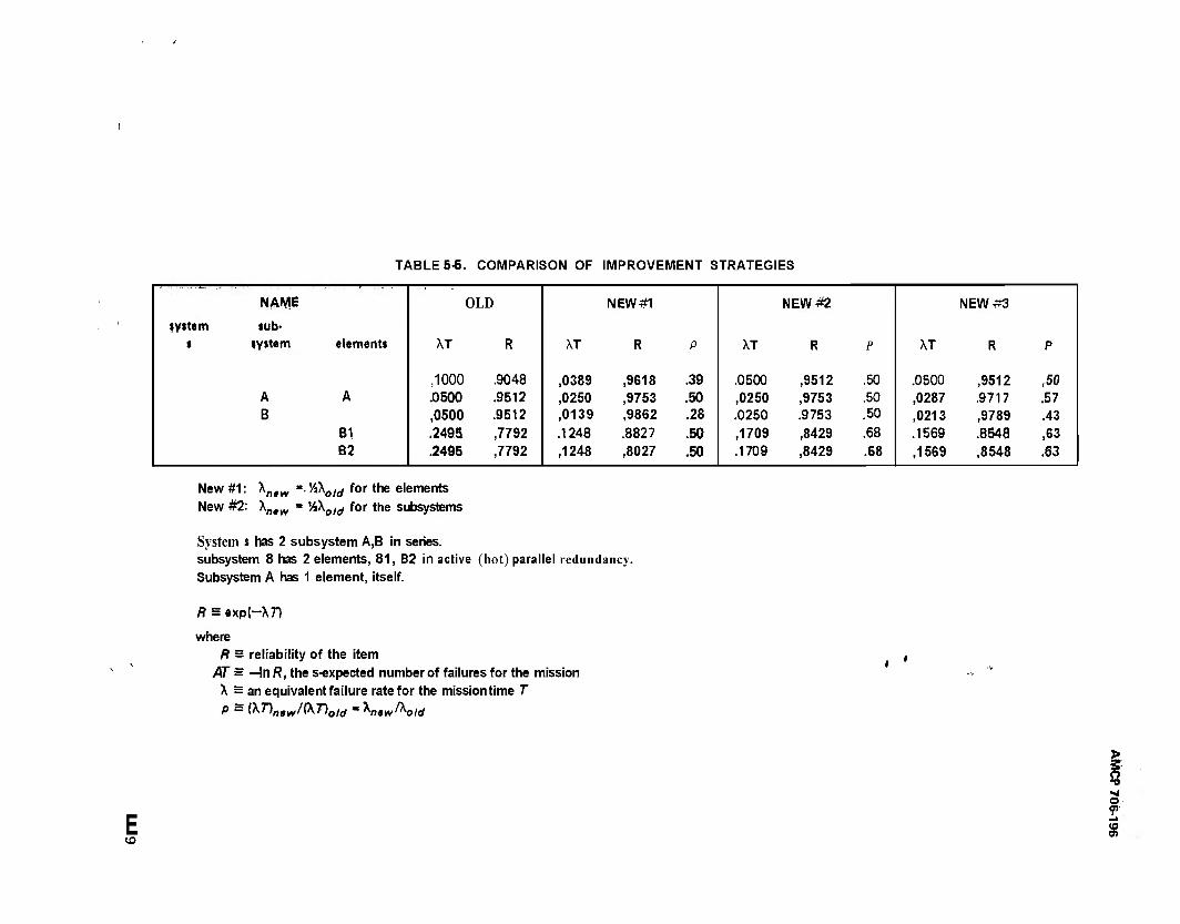
TABLE 5-6, COMPARISON OF IMPROVEMENT STRATEGIES

NAME OLD NEW#1 NEW #2 NEW #3

«yttem tub- t iv»tem elements XT R XT R P XT R P XT R P

,1000 .9048 ,0389 ,9618 .39 .0500 ,9512 .50 .0500 ,9512 ,50 A A .0500 .9512 ,0250 ,9753 .50 ,0250 ,9753 .50 ,0287 .9717 .57 B ,0500 .9512 ,0139 ,9862 .28 .0250 .9753 .50 ,0213 ,9789 .43

B1 .2493 ,7792 .1248 .8827 .50 ,1709 ,8429 .68 .1569 .8548 ,63 B2 .2495 ,7792 ,1248 ,8027 .50 .1709 ,8429 .68 ,1569 ,8548 .63

New#1: \new

New #2: Xn#vv

■ '/iX0/cy for the elements V4Xo/d for the subsystems

System s has 2 subsystem A,B in series. subsystem 8 has 2 elements, 81, B2 in active (hot) parallel redundancy. Subsystem A has 1 element, itself.

R s exp(—\T)

where R & reliability of the item

AT s —In R, the s-expected number of failures for the mission X s an equivalent failure rate for the missiontime T f> s (^71„9vv/(\71oW 'Ktm^-old

<o

■a

o 9 s

AMCP 706-196

A number of different optimization techniques are available that work well for many different types of problems. The methods are general; however, only a limited number of variables will be considered, permitting the use of simple examples. Also, from a practical point of view, limiting the analysis to a few variables results in mathematically tractable problems whose results can be visualized by the engineer.

An allocation of subsystem reliability with constraints requires the existence of data or formulas that relate the constrained variables to reliability, i.e., the cost (or weight, etc.) of system alternatives of different reliabilities must be computable. This is usually the area of greatest uncertainty in system design, and the cost data frequently are obtained by means of a rough guess. Although the techniques described are general, the engineer must keep in mind the fact that the results produced are very sensitive to the quality of the input data.

5-2.7.1 Simple Redundancy Allocation With a Single Constraint

As the complexity of weapon systems increases, their reliabilities tend to decrease, One method for coping with this problem is to design reliable systems using less reliable subsystems in redundant configurations,

The simple technique in this paragraph describes a method for maximizing system reliability subject to a single constraint such as cost; it also can be extended to multiple constraints. An abundant literature has been developed that describes the techniques used for redundancy allocation, such as Lagrange multipliers and dynamic programming.

Example Problem No. procedure (Rafs.7 to 23).

7 jHustzatES the

5-2.7.2 Dynamic Programming Allocation

Dynamic programming allocation (Ref. 10) is another useful procedure when system reliability must be allocated to the subsystems in the face of constraints on such factors as weight and cost. The dynamic programming approach can be most useful because it can be

implemented with a simple algorithm that consists of only arithmetic operations. Some advantages of the dynamic programming approach are:

(1) Large problems can be solved with a minimum number of calculations (this "minimum" may be very large for a complex system).

(2) There is always a finite number of steps required in computing'&n optimum solution.

(3) There are no restrictions of any kind on the form cf the functional expressions for computing reliability or the form of the cost estimating equations. Nonlinear functions can be used if required.

The dynamic programming algorithms provide a guide through the maze of possible alternate calculations that may arise when big systems are being analyzed. The dynamic programming approach also can be applied to the problem of reliability optimization of redundant systems with repair. The use of the dynamic programming algorithm does not in any way remove the requirement for computing the reliability and cost for each system configuration. However, it minimizes the total number of calculations by rejecting those configurations that would result in a decreasing reliability or in costs exceeding the cost constraints, etc.

Many algorithms can be developed to solve dynamic programming problems, Gener- ally, the algorithm chosen should be the one that is more efficient, i.e., finds the solution with the least number of iterations. For any reasonably large system a large number of calculations are required; therefore, the engineer must consider using the computer and should consult the sysban programmers to findvfoat programs are readily available.

5-2.7.3 Minimization of Effort Algorithm

The minimization cf effort algorithm technique (Ref. 24) can be used to allocate reliability requirements to the subsystems in a way that minimizes the engineering design effort (cost, man-hours, etc.) required to achieve overall systsn reliability. We are not applying a constraint to cost by merely trying

3

n

5-20

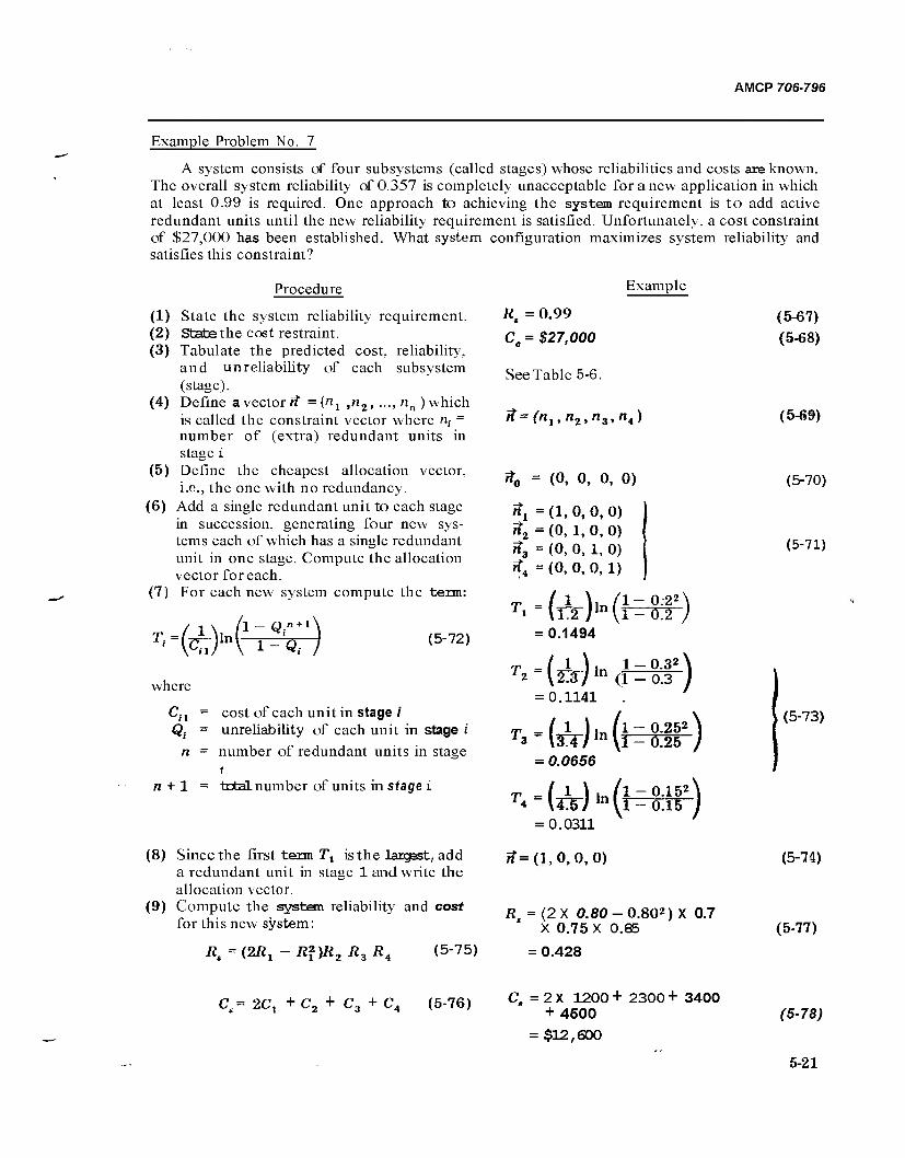
AMCP 706-796


A system consists of four subsystems (called stages) whose reliabilities and costs are known. The overall system reliability of 0.357 is completely unacceptable for a new application in which at least 0.99 is required. One approach to achieving the system requirement is to add active redundant units until the new reliability requirement is satisfied. Unfortunately, a cost constraint of $27,000 has been established. What system configuration maximizes system reliability and satisfies this constraint?

Procedure

(1) State the system reliability requirement. (2) State the cost restraint. (3) Tabulate the predicted cost, reliability,

and unreliability of each subsystem (stage).

(4) Define avectorff ={n1 ,n2, ...,nn)which is called the constraint vector where n, = number of (extra) redundant units in stage i

(5) Define the cheapest allocation vector, i.e., the one with no redundancy.

(6) Add a single redundant unit to each stage in succession, generating four new systems each of which has a single redundant unit in one stage. Compute the allocation vector for each.

(7) For each new system compute the term:

T,= («Ö In Qi n + l

Q, (5-72)

where

Cn = cost of each unit in stage / Q. - unreliability of each unit in stage i

n = number of redundant units in stage 1

n + l = total number of units in stage i

(8) Since the first term 7\ is the largest, add a redundant unit in stage 1 and write the allocation vector.

(9) Compute the system reliability and cost for this new system:

Example

Rt = 0.99

Ce = $27,000

See Table 5-6.

rt=(n1,n2,n3,n4)

% = (°. o. o. 0)

nx = (1, 0, 0, 0) h*2 = (0, 1, 0, 0) it3 = (0, 0, 1, 0) X4 =(0,0,0,1)

(5-67)

(5-68)

(5-69)

(5-70)

(5-71)

= 0.1494

T2 = (^jln (1 - 0.3* ) = 0.1141 .

T3 = (sx)ln (l - lit) = 0.0656

(5-73)

Rt = (2RX R*)R2R3R4 (5-75)

= 0.0311

7f=(l,0,0,0)

fi =(2X 0.80 -0.802)X 0.7 X 0.75 X 0.85

= 0.428

(5-74)

(5-77)

C = 2C, + c2 + c3+c4 (5-76) C, = 2 X 1200 + 2300 + 3400 + 4500

= $12,600

(5-78)

5-21

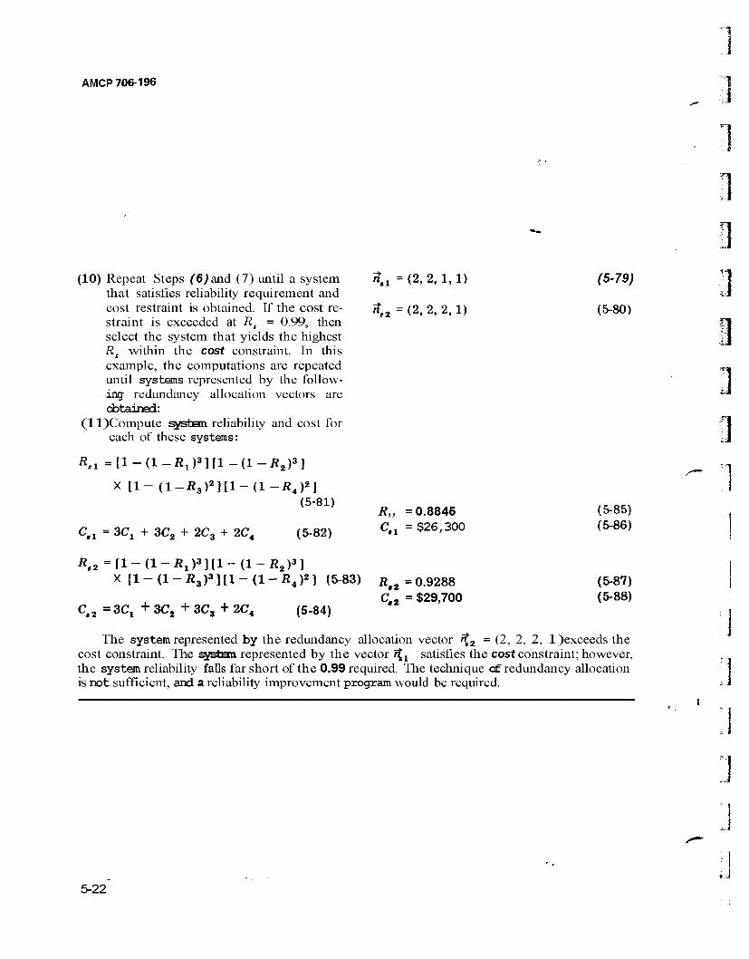
AMCP 706-196 1

. i

1

(10) Repeat Steps (6) and (7) until a system nti = (2, 2, 1, 1) (5-79) that satisfies reliability requirement and cost restraint is obtained. If the cost re- 7?f2 = (2, 2, 2, 1) (5-80) straint is exceeded at Rt = 0.99, then select the system that yields the highest Rs within the cost constraint. In this example, the computations are repeated until systems represented by the following redundancy allocation vectors are obtained:

(ll)Compute system reliability and cost for each of these systems:

Rtl =[1-(1-Rl)3}[l-(1-R2)

3)

X [l-(l-Ä3)2][l-(l-ii4)2]

c.i = 3Ci + 3C2 + 2C3 + 2C4

(5-81) R„ = 0.8845

(5-82) C.x = $26,300

(5-85) (5-86)

Ä.aMl-d-.R^Hl-U-Ä,)3] X [1 - (1 - R3 )S ] [i - (i _ R4 )»] (5.83) Ri2 = 0.9288 (5-87)

c.2 = 3Ci + 3C2 + 3C3 + 2C4 (5-84) C,2 = $29,700 (5-88)

The system represented by the redundancy allocation vector ft2 = (2, 2, 2, l)exceeds the cost constraint. The system represented by the vector ^j satisfies the cost constraint; however, the system reliability falls far short of the 0.99 required. The technique cf redundancy allocation is not sufficient, and a reliability improvement program would be required. :i

j

5-22

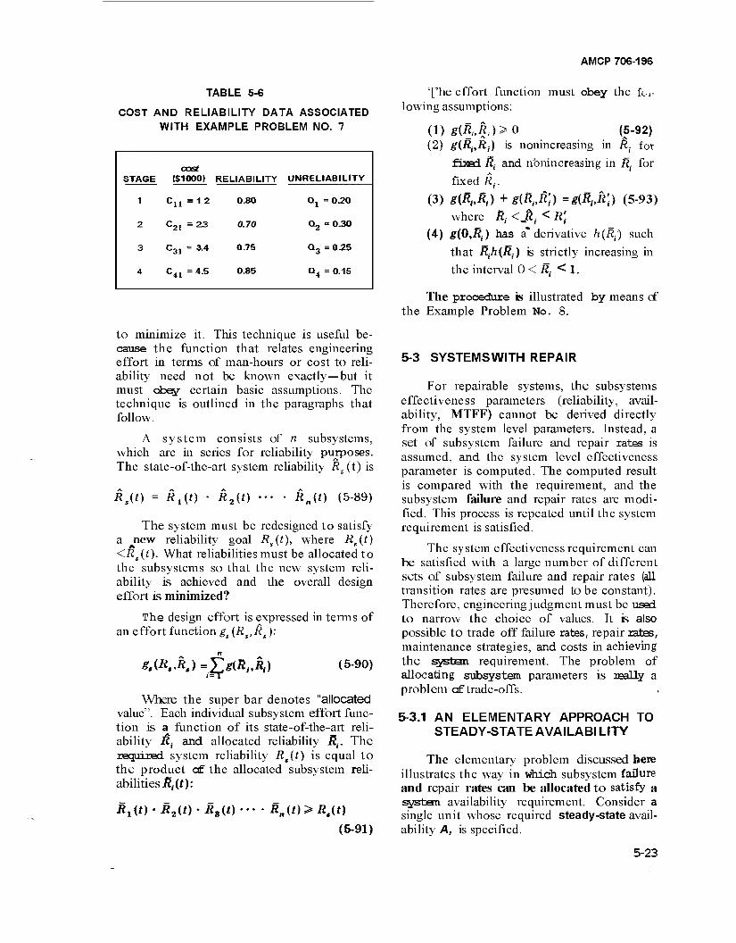
AMCP 706-196

TABLE 5-6

COST AND RELIABILITY DATA ASSOCIATED WITH EXAMPLE PROBLEM NO. 7

cost STAGE

1

($1000)

C„ =12

RELIABILITY

0.80

UNRELIABILITY

Qj = 0.20

2 C21 = 23 0.70 Q2 = 0.30

3 C31 - 3.4 0.75 Q3 = 0.25

4 C41=4.5 0.85 Q4 = 0.15

to minimize it. This technique is useful because the function that relates engineering effort in terms of man-hours or cost to reliability need not be known exactly—but it must obey certain basic assumptions. The technique is outlined in the paragraphs that follow.

A system consists of n subsystems, which are in series for reliability purposes. The state-of-the-art system reliability Rs (t) is

Rs{t) = R^t) - R2(t) RJt) (5-89)

The system must be redesigned to satisfy a new reliability goal R,(t), where RK(t) <Rs(t). What reliabilities must be allocated to the subsystems so that the new system reliability is achieved and the overall design effort is minimized?

The design effort is expressed in terms of an effort function gs {Rs,Rt )'■

g,(R,.Rt) =^giR„R,) (5-90)

Where the super bar denotes "allocated value". Each individual subsystem effort function is a function of its state-of-the-art reliability Rt and allocated reliability R~t. The required system reliability Rs(t) is equal to the product at" the allocated subsystem reliabilities R,(t):

R^t) • R2(t) ■ Ra{t) Rjt)>Rt(t)

(5-91)

'['he effort function must obey the following assumptions:

(1) g(R:,Ri)>0 (5-92) (2) giR^Rj) is nonmcreasing in R. for

fixBd R( and nbnincreasing in R. for

fixed Rr

(3) g(R,,Rt) + g(M,:) =*tM;> (5-93) where fi,- <ßi < R\

(4) g{OyR{) has a* derivative h(Rj) such

that Rjhföj) is strictly increasing in

the interval 0 < ß,- < 1.

The procedure is illustrated by means of the Example Problem No. 8.

5-3 SYSTEMSWITH REPAIR

For repairable systems, the subsystems effectiveness parameters (reliability, availability, MTFF) cannot be derived directly from the system level parameters. Instead, a set of subsystem failure and repair rates is assumed, and the system level effectiveness parameter is computed. The computed result is compared with the requirement, and the subsystem failure and repair rates are modified. This process is repeated until the system requirement is satisfied.

The system effectiveness requirement can be satisfied with a large number of different sets of subsystem failure and repair rates (all transition rates are presumed tobe constant). Therefore, engineering judgment must be used to narrow the choice of values. It is also possible to trade off failure rates, repair rates, maintenance strategies, and costs in achieving the sygten requirement. The problem of allocating subsystem parameters is really a problem cf trade-offs.

5-3.1 AN ELEMENTARY APPROACH TO STEADY-STATE AVAILABILITY

The elementary problem discussed here illustrates the way in which subsystem failure and repair rates can be allocated to satisfy a sysbart availability requirement. Consider a single unit whose required steady-state availability A, is specified.

5-23

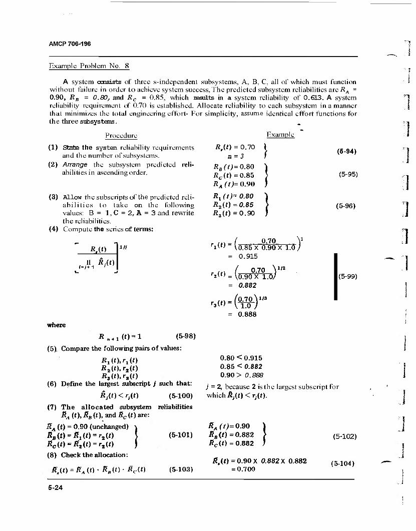
AMCP 706-196


A system cmsists of three s-independent subsystems, A, B, C, all of which must function without failure in order to achieve system success, The predicted subsystem reliabilities are RA = 0.90, RB = 0.80, and Rc = 0.85, which results in a system reliability of 0.613. A system reliability requirement of 0.70 is established. Allocate reliability to each subsystem in a manner that minimizes the total engineering effort- For simplicity, assume identical effort functions for the three subsystems.

Procedure

(1) State the system reliability requirements and the number of subsystems.

(2) Arrange the subsystem predicted reliabilities in ascending order.

(3) Allow the subscripts of the predicted reliabilities to take on the following values: B= 1, C = 2, A = 3 and rewrite the reliabilities.

(4) Compute the series of terms:

*.(*)

n Rjit)

ifj

where

R n+ 1 (0 = 1 (5-98)

(5). Compare the following pairs of values:

R1(t),r1(t) iJ2(0,r2(0 R3{t),ra(t)

(6) Define the largest subscript / such that:

Äi(0<'>(0 (5-100)

(7) The allocated subsystem reliabilities RA(t),RB(t), and Rc(t) are:

KA (t) = 0.90 (unchanged) \ JZj(t)«£1(')'sr1(t) } (5-101) *c(') = #8(0 = r2(0 ) (8) Check the allocation:

Ä.(0 = ^(0-Äj,(0-Äc(0 (5-103)

Example

ß,(0 = 0.70 n = 3

RB(t)= 0.80 Rc(t) =0.85 RA (t)= 0.90

Rx (t)~ 0.80 R2(t) =0.85 R3{t) = 0.90

I

!

i

(5-94)

(5-95)

(5-96)

... _ ( 0.70 V riW" V0.85X 0.90 X 1.0/

= 0.915

r m ( JP-70 V/2 r2^f = \0.90X 1.0/

= 0.882

= 0.888

(5-99)

0.80 < 0.915 0.85 < 0.882 0.90 > 0.888

j = 2, because 2 is the largest subscript for which ftj(t) < rj(t).

RA (0=0.90 SB(t)= 0.882 Rc(t) = 0.882 } £,(f) = 0.90 X 0.882 X 0.882

= 0.700

(5-102)

(5-104)

5-24

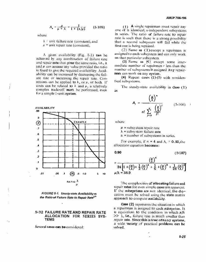
AMCP 706-196

H + \ 1 + (X/JI) (5-105)

where

X - unit failure rate (constant), and M = unit repair rate (constant),

A given availability (Fig. 5-1) can be achieved by any combination of failure rate and repair rate that gives the same ratio, i.e., A and p can assume any value provided the ratio is fixed to give the required availability. Avail- ability can be increased by decreasing the failure rate or increasing the repair rate. Con- straints can be applied to X, or ß, or both. If costs can be related to X and ju, a relatively complex trade-off must be performed, even for a simple 1 -unit system.

AVAILABILITY .99

.5

.2

>y EXAMPLE

■1

(1) A single repairman must repair any one of n identical, s-independent subsystems in series. The ratio c£ failure rate to repair rate is such that there is a strong possibility that a second subsystem will fail while the first one is being repaired.

(2) Same as (1) except a repairman is assigned to each subsystem and can only work on that particular subsystem.

(3) Same as f4) except some intermediate number of repairmen r less than the number of subsystems is assigned. Any repair- nan can work on any system.

(4) Repeat cases (l)-(3) with noniden- tical subsystems.

The steady-state availability in Case (1) is:

A, = (*)"

" (ir)' }=0 J'

(5-106)

where

V = subsystem repair rate X = subsystem failure rate n = number of subsystems in series.

For example, if n = 4 and A, allocation equation becomes:

0.90

0.90,the

(5-107)

HtHft)' (Ö4

24 1 + 2 1

(*)' .01 .05 .1 (25) .5 1.0 5 10 ßfk = 38.9

JW\ RATIO

FIGURE 5-1. Steady-state Availability vs the Ratio of Failure Rate to Repair Rate2 6

5-32 FAILURE RATE AND REPAIR RATE ALLOCATION FOR SERIES SYS- TEMS

Several cases can be considered:

The complexities cf allocating failure and repair rates for even simple cases are apparent. If the subsystems are not identical, the do- cation must be solved using the state matrix approach to compute availabUity.

Case (2) represents the situation in which a repairman is assigned to each subsystem. It is equivalent to the condition in which p/X » 1, i.e., failure rate is much smaller than repair rate. Since this is true of many systems, a wide -variety of practical problems can be solved.

5-25

AMCP 706-196

The steady-state availability of a series system of n identical, s-independent subsystems is

(5-108) ^ = V=[TTW]

where

A, = system steady-state availability Aj = subsystem availability n = number of subsystems

Example Problem No. procedure.

9 illustrates the

5-3.3 A SIMPLE TECHNIQUE FOR ALLO- CATING STEADY-STATE AVAIL- ABILITY TO SERIES SYSTEMS

A procedure similar to the method in par. 5-2.2 for allocating reliability without repair can be used when the ratio yJ = \/jU; *■> 0.1 for subsystem;', for all j. The accuracy of the method increases as ?y decreases. The availability of a series system with subsystems whose failures and repairs are all s-independent is:

A, =

1 + X>/ (5-115)

where

7y = ratio for subsystem / with all y f < 0.1 n = number of subsystems in series

The system yM :

y,,oid =Ti +72 + * • • +yn (5-116)

A relative weighting factor Wf can be computed from:

^ ">;/7..ow (5-117)

The new system is similar in design to the old, and the relative weighting factors are the same for each new subsystem.


5-3.4 FAILURE AND REPAIR RATE AL- LOCATIONS FOR REDUNDANT SYSTEMS

A system comprising several stages c£ redundant subsystems whose X/ju ratio is less than 0.1 can be treated as if the stages were s-independent. The system steady-state availability A, is

A, = At

where

A2 • A3 " ' A, (5-131)

Aj = the availability of stagej.

This is equivalent to treating each stage as if it had a repairman assigned to it. It is also equivalent to saying that a single repairman is assigned to the system, but that the probability of a second failure occurring while the first is being repaired is very small. If the stages are not s-independent, the system availability must be computed .by the state matrix approach. In either case, the system requirement can be obtained with a range of failure and repair rates. Trade-offprocedures must be used to determine the best set of these parameters.

The availability of a systaem of n identical units where at least m cf n must be operating &r the system to be operating is:

n (5-132)

where

V = X = n =

unit repair rate (constant) unit failure rate (constant) total number of units

m = minimum number cf units which must be up for the system to be up.

Availabilities can be computed as a function of repair rate to failure rate ratios for systems cf up to five redundant units in parallel using Figs. 5-2through 5-5 (Ref. 25).

If the subsystems in the stage are not identical, state matrix techniques can be used to compute availability.

5-26

AMCP 706-196


A system consists of three identical, s-independent subsystems connected in series. The availability requirement is 0.99, and the repair rate is limited to 0.3 per hr. What is the minimum failure rate which must be allocated to each subsystem to satisfy the system requirement? A repairman is assigned exclusively to each subsystem.

Procedure

(1) State the system availability requirement. (2) Compute the availability of each sub-

system by Af = (A,)"" (5-110)

(3) For each subsystem compute the ratio X/ju by:

2L A (5-112)

Example

A, = 0.99

A, =0.991'3

= 0.99666

X_ 1 H 0.99666

= G. 00336

- 1

(5-109)

(5-111)

(5-113)

(4) Compute X by Eq. 5-113 with u - 0.3 per hr. The final answer is rounded cff" to 2 significant figures to avoid implying too much accuracy.

X = 0.00336 X

= 1.0 per 10 3 per hr) (5-114)

Case (3) represents a much more complex problem. Availability must be computed using the state matrix approach. An optimum allocation requires the use cf dynamic programming algorithms.

5-27

AMCP 706-196


A system consisting cf two s-independent subsystems has an availability of 0.90. Subsystem 1 has an availability of 0.97, and subsystem 2hasan availability of 0.93. Anew system, similar in design to this one, must meet a required 0.95 availability. What are the new subsystem availabilities and ratios of failure-to-repaix rate?

Procedure

(1) State the availability requirement A, of the new system.

(2) Compute the sum ys of the y-ratios for the old system:

y,,oiä=yi +T2 (5-ii9)

(3) Compute the relative weights W{ by Eq. 5-117.

Example-

A, =0.95

Von =0.0309 + 0.0753 = 0.1062

ii/ - 0-0309 wi ~ 0.1062

(5-118)

(5-120)

(5-121) = 0.291

(4) Compute an overall ys for the new system by:

T. = T (5-123)

Wn _ 0.0753

0.1062 = 0.709

= 0.0526

(5-122)

(5-124)

(5) Compute the allocated 7;- for each subsystem of the new design by:

y, = vrp. (5-125)

fj = 0.291 X 0.0526 = 0.0153

f2 = 0.709 X 0.0526 = 0.0373

(5-126)

(6) Compute the availabilitiesÄ} allocated to each subsystem by:

*>-T (5-127)

î "Ii" 0.0153 = 0.985

A, = 1 + 0.0373 = 0.964

(5-128)

(7) Check the allocated availability A, of the new system by:

As = Ä • Ä2 (5-129)

A, =0.985 X 0.964 = 0.950 (5-130)

Since the allocated ratios are known, the trade-off studies can be performed. ^

5-28

AMCP 706-196

m = minimum number of units which must be up tor

the system to be up.

n = total number of units

m = minimum number of_units which must be up for the system to be up

n " total number of units.

a.l-<

10'

10

10'

2 10*

Q 1)

O o

10'

10

1 1

m A

Solution for 1 , Ml" n + — I \

r. = 2

"SsV'" - 1

10 s 10" 10 ■' 10;

Unavailability 10

Copyrighted by Prentice-Hall, Englewood Cliffs. NJ., 1963. Reprinted from System Reliability Engineering by permis- sion.

FIGURE 5-2. Repair Rate to Failure Rate Ratio vs Unavailability fn V'"

■10"

10*

| 10*

CO »*- O

£ 103

a

° 10' o

10

Solution for 1- m A

V rri 3

(1

n = .1

*X- m e 2

„m - 1

10 10" 10"'

Unavailability

10 10

Copyrighted by Prentice-Hall, Englewood Cliffs. NJ., 1963. Reprinted from System Reliability Engineering by permis- sion.

FIGURE 53. .lepair Rate to failure Rate Ratio vs

Unavailability (n = 3}-s

5-29

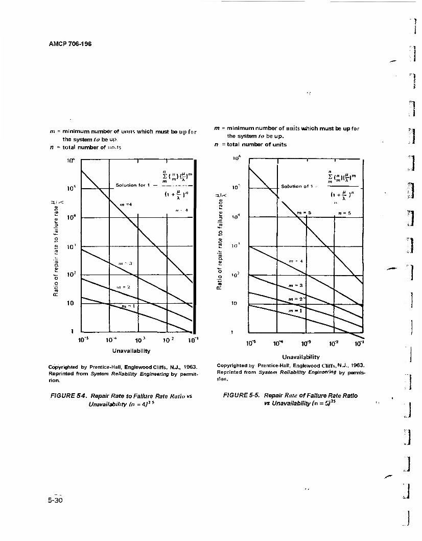
AMCP 706-196

1 m = minimum number of units which must be up for

the system to be up. n - total number of units

10*

10s

3.! SC

CO

104

o

2 10'

o o

cc

10-'

10

Solution

n

m for 1 — —

0£>m

^V^ m -4

(

» - -1

V"' "■ '■*

.n = 2

Vjn; 1

10 s 104 10* 103 10"'

Unavailability

Copyrighted by Prentice-Hall, Englewood Cliffs, N.J., 1963. Reprinted from System Reliability Engineering by permit rion.

m = minimum number of units which must be up for the system to be up.

n = total number of units

10"

10 =L!-<

Ü 4

*ni

o

a

O ,

+-»

CC

10

10-

\ _

1

f 1 -

5

I

\ (i

n = 5

"x^ m = 4

\

■«^»n = 3 \

^^^/7l » 1

10^ 10^ 10^ 10'1

Unavailability

Copyrighted by Prentice-Hall, Englewood Cliffs, N.J-. 1963. Reprinted from System Reliability Engineering by permis-

]

FIGURE 54. Repair Rate to Failure Rate Ratio vs

Unavailability (n = 4;2 s

FIGURE 5-5. Repair Rate of Failure Rate Ratio vs Unavailability (n = 5)ls

.]

5-30

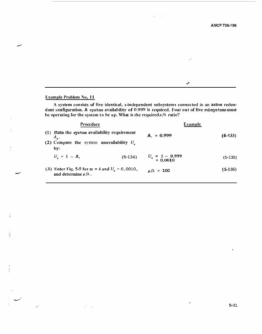
AMCP 706-196

Example Problem No, 11

A system consists of five identical, s-independent subsystems connected dn an active redundant configuration. A system availability of 0.999 is required. Four out of five subsystems must be operating for the system to be up. What is the requiredP/A ratio?

Procedure Example

(1) State the system availability requirement

(2) Compute the system unavailability Us

by:

U, = l-A, (5-134) U. = 1 -o 0.999 (5.135)

(3) Enter Fig. 5-5 form = 4 and Ut = 0.0010, /x = 100 (5-136) and determine /i /A .

5-31

AMCP 706-196


5-3.5 RELIABILITY WITH REPAIR AND INSTANTANEOUS AVAILABILITY

In general, reliability with repair and instantaneous availability only can be computed using the state matrix approach. Except for very simple systems, algebraic expressions that represent reliability without repair and instantaneous availability as functions of subsystems repair failure and repair rates are extremely cumbersome and cannot be manip- ulated readily. The engineer must define the transition matrix of the system in order to implement these procedures.

REFERENCES

1. MIL-HDBK-217, Reliability Stress and Failure Rate Data for Electronic Equip- ment.

2. W. H. Von Alven, Ed., Reliability Engi- neering, Prentice-Hall, Englewood Cliffs. N.J., 1964.

3. Reliability of Military Electronic Equip- ment, Advisory Group on Reliability of Electronic Equipment (AGREE), Office of the Assistant Secretary of Defense, U S Government Printing Office, Wash- ington, D.C., June 1957.

4. H. S. Balaban, et ah, The Allocation of System Reliability. Vol. II. Step-by-step Reliability Allocation Procedure, ASD TDR 62-20, Aeronautical Systems Div., USAF, Wright-Patterson AFB, Ohio, June 1962.

5. F. E. ixfersh, "Inherent Reliability De- sign Practices, Reliability Apportion- ment", Reliability Control in Aerospace Equipment Development, Society of Automotive Engineers, Technical Pro- gress Series, SAE, N.Y., 38 (1963).

6. Cost-EffectivenessSupplement, Vol. HI, AFSC-TR-65-4, Weapons System Effec- tiveness Industry Advisory Committee (WSEIAC), January 1965.

7. L. A. Aroian, Maximization of the Reliability of a Complex System by the Use of Items in Sequence,

ST4TM/60-0000-00034, Space Tech- nology Laboratories, Los Angeles, California.

8. R E. Barlow and L. (^.Hunter, "Criteria for Determining Optimum Redun- dancy", IRE Transactions on Reliability and Quality Control, RQC-9, 73-7 (April 1960).

9. R. E. Barlow and F.-Proschan, Mathe- matical Theory of Reliubility, John Wiley and Sons, N.Y., 1965.

10. R. Bellman and S. Dreyfus, "Dynamic Programming and the Reliability of Multicomponent Devices", Operations Research, 200-6 (April 1958).

11. G. Black and F. Proschan, "On Optimal Redundancy", Operations Research, 581-8(1959).

12. H. Everett, "Generalized Lagrange Mul- tiplier Method for Solving Problems of Optional Allocation of Resources", Operations Research, 399-417 (May 1963).

13. B. J. Flehinger, "Reliability Improve- ment Through Redundancy at Various System Levels", IBM Journal (April 1958).

14. R. Gordon, "Optimum Redundancy for Maximum System Reliability", Opera- tions Research, 229-43 (April 1957).

15. J. D. Kettelle, Jr., "Least-Cost Alloca- tions of Reliability Investment", Opera- tions Research, (March 1962).

16. J. Luttschwager, "Dynamic Program- ming in the Solution of a Multistage Reliability Problem", Journal of Indus- trial Engineering, 69-175 (1964).

17. G. E. Neuner and R. N. Miller, "Re- source Allocation for Maximum Reli- ability", Proceedings of the 1966 Annual Symposium on Reliability, 332-46 (1966).

18. F. Proschan and T. A. Bray, "Optimum Redundancy Under Multiple Con- straints", Operations Research, 800-14 (September 1965).

19. G Pugh, "Lagrange Multipliers and the Optimal Allocation of Defense Re- sources", Operations Research, 543-67 (July 1964).

20. M. Sasaki, "A Simplified Method of Obtaining Highest System Reliability",

1

5-32

AMCP 706-196

Proceedings of the Eighth National Symposium on Reliability and Quality Control, 489-502 (January 1962). 24.

21. M. Sasaki, "An Easy Allotment Method Achieving Maximum System Reliabil- ity", Proceedings of the Ninth National Symposium on Reliability and Quality Control, 109-24 (January 1963). 25.

22. R. B. Thakkar and R. C. Hughes, "Aero- space Power Systems: Maximizing Reli- ability with Respect to Weight", IEEE 26. Transactions on Aerospace, 528-34 (April 1964). 27.

23. L. Webster, "Choosing Optimum System Configurations", Proceedings of the Tenth National Symposium on Reliabil-

ity and Quality Control, 345-59 (January 1964). A. Albert, A Measure of the Effort Re- quired to Increase Reliability, Technical Report No. 43. Applied Mathematics and Statistics .Laboratory, Stanford University, 1958. G. H. Sandier, System Reliability Engi- neering, Prentice-Hall, Englewood Cliffs, N.J., 1963. NAVWEPS 00165-502, Handbook of Reliability Engineering, June 1964. M. L. Shooman, Probabilistic Reli- ability: An Engineering Approach, McGraw-Hill Book Co., N.Y., 1968.

5-33

AMCP 706-196

CHAPTER 6 HUMAN FACTORS

6 0 LIST OF SYMBOLS

Cdf = Cumulative distribution function pdf = probability density function

Pr{' } = probability of . - . Pr{-I-}'= conditional probability. The "I"

is read as "given that". Sf = Survivor function: Sf = 1 — Cdf

6-1 INTRODUCTION

All systems of concern in this Handbook are of, by, and for humans. Analyses of the behavior and needs of humans are among the more controversial of the sciences; thus it is no surprise that there are several competing approaches to the handling and identification of people problems. Refs. 22 and 23 analyze some of these approaches; but even there, some disagreements exist about the compar- isons themselves. It is convenient to classify four types of human interactions with a system; the classes are convenient, but not sharp and clear cut:

(1) Design and production of a system (2) Operators and repairers as mechan-

ical elements (human engineering) (3) Q«-THICIS and repairers as decision

elements (human performance reliability) (4) Bystanders (this classification is not

considered further because it is largely a safety matter, not reliability).

An example of the fuzziness between classes is an operator's having to decide what to do, then doing it; there is considerable interaction between the two activities.

An initial appraisal of the man/machine system must consider such aspects as: allocation of functions (man vs machine), automation, accessibility, human tasks and their performance metrics, human stress characteristics, information presented to the human and the reliability of inferences coupled with the decisions on the basis of such information, and accessibility. The answers to these questions and the study of man/machine interactions and interfaces fall within the field variously called human factors, human engineering, or ergonomics (Ref. 28).

This field is defined in MIL-STD-721 (Ref. 7) as: "A body of scientific facts about human characteristics, The term .covers all biomedical and psychosocial considerations; it includes, but is not limited to, principles and applications in the area of human engineering, personnel selection, training, life support, job performance aids, ancL-human performance evaluation."

Human factors engineering is applied to research, development, test, and evaluation of systems to insure efficient integration of man into the system environment. This integration is intended to increase and preserve human and machine performance in the system during operation, control, maintenance, and support activities. Human engineering, therefore, becomes an active participant in the system engineering process and, consequently, must be weighed against safety, reliability, maintainability, and other system parameters to obtain trade-offs providing increased system effectiveness. During the concept formulation phase, human factors data are used in predictions of system effectiveness and for initial function allocation studies. Human reliability studies during the contract definition phase are included in system reliability calculations, maintainability time and performance evaluations, system and subsystem safety analyses, and specific human engineering design criteria. The engineering development and production phases provide specific man/machine interactions for amplification of previous studies, isolate and define trade-off and interaction problems not previously identified, and allow verification of prior design decisions on reliability, maintainability, safety, and other system parameters which interact with human factors.

An annotated bibliography of 27 items taken from NTIS reports is listed in Appendix C.

6-2 DESIGN AND PRODUCTION

On the average, people are average. This truism is often fbrgottenby systaan designers, planners, and managers- Each wants to have well-above-average people in the tasks he is

6-1

AMCP 706-196

arranging. System designers do pay some attention to this problem when considering operators and repairers. But rarely is it considered in the design and manufacturing areas, although industrial and manufacturing engineers do deal with it as they are able in their constricted region of operation.

Beginning with the conception of a system, it is important to realize the limitations of the people involved all through the life cycle. Large organizations cannot and will not change rapidly, even though there is a management decree that the change will occur. People cannot adequately plan complete changes in a way of life or of work—there are toomany unknown, unforeseen factors.

A system and its subsystems ought to be straightforward to design. Interfaces between subsystems ought to be as simple as possible. The more complexity, the more likely <=m-rg axe to occur. Checklists are a valuable aid to designers. Design reviews and other product reviews (Chapter ll)help to overcome hum an limitations by putting some redundancy in the design system.

The designer of an equipment needs to consider haw it will be produced; e.g., what kinds of quality control will be necessary, what machines/operators will actually perform a task. Reducing the occasion of very similar appearing parts, but which are different, can help avoid mistäss. A design that can accept looser tolerances might be better than one viiich requires tight tolerances, even though the latter would perform better if everything were right.

The designer needs to consider how the equipment actually will be repaired in the field. For example, if a repair when done right takes about 8 hr, and when done almost-right takes 1 hr, which way vUL it be done under the pressures cf understaffed maintenance crews many c£ whom are inexperienced? One cannot expect that field service personnel will have the knowledge about the systen that the designers have. Even where the situation is understood, the of£icer-in-charge under the pressures of command might well choose to have the almost-right repair that takes only I hr. The designer must always keep in mind that the equipment will be used and repaired

by ordinary people who have other things in mind than "babying" the equipment. He must realize the difference between what people actually will do, and what he thinks they ought to do.

if the familiar production processes in a plant will have to change, then a quality assurance effort must be implemented to be sure the system does change anjj that it changes correctly.

A Cause-Consequence chart (Chapter 7) is a good tool for viewing the design-production process. It allows one to look at:

(1) What can go wrong (causes) (2) How likely it is to go wrong (3) What happens when it does go wrong

(consequences) (4) How to alleviate the severe conse-

quences.

Anywhere people are involved in doing something, the Cause-Consequence chart-even a very simple one—can help locate potential people problems.

System planners should be aware of the impact of administrative policies on the reliability of systems. In Ref. 10 it is shown that many reported failures were not the result of either faulty design or human error (for the Air Force F-106 avionics systems), but were "required" by the procedural environment. Ref. 10 ought to be read by every ^stsn planner.

6-3 HUMAN ENGINEERING

This area deals largely with motor responses of operators and with varied human physical capabilities. Itefs. 1-6 cover this area adequately. Typical constraints are that:

(1) An operation ought to be within the physical capabilities of the central 95% of the potential operators,

(2) A person is not required to do something that his coordination will not allcwhim to do, e.g., something akin to patting his head with the left hand while rubbing his chest with the right hand.

(3) Real people cannot easily use, read, and 'respond to controls and displays, especially in times of psychological stress.

:?

6-2

AMCP 706-196

Mock-ups under realistic conditions are very helpful in uncovering forgotten constraints. For example, if an equipment must be used at night in extremely cold weather, have a person try to use it in a freezing, poorly lit room for several hours.

Military standards, regulations, specifications, and other publications contain guidelines, policies, and requirements for human factors and human engineering. For example, Army requirements and policies for human engineering programs are presented in Refs. 8-10. MILSTD-1472 (Ref. 1), the MIL STD-803 series (Refs. 2-4), and MIL-H- 46855 (Ref. 5) give design criteria, requirements, and definitions for human engineering in military systems. Standardization, automation, visual and auditory displays, controls, labeling, workspace design, maintainability, remote handling devices, safety hazards, and environmental requirements are some of the subjects treated in these sources (Refs. 1-5). Definitions of human factors terms are also found in MTLSTD-721 (Ref. 7).

6-4 HUMAN PERFORMANCE RELI- ABILITY

Fhe analysis of human factors recognizes that both human and machine elements can fail, and that just as equipment failures vary in their effects on a system, human errors can also have varying effects on a system, hi some cases, human errors result frcm an individual's action, while others are a consequence of system design or manner of use. Some human errors cause total system failure or increase the risk of such failure, while others merely create delays in reaching system objectives. Fhus, as with other system parameters, human factors exert a strong influence on the design and ultimate reliability of all systems having a man/machine interface. A good summary and critical review of human performance reliability predictive methods is given in Ref. 22 which is a surcrrazy of Ref. 23. Both references contain excellent bibliographies. Fable 6-1 is taken from Ref. 22 and lists the available predictive methods-

TABLE6-1. LIST OF PREDICTIVE METHODS

OPERABILITY METHODS

A. Analytic

'1. American Institute for Research (AIR) Data

Store

'2. THERP-Technique for Human Error Rate

Prediction

'3. TEPPS-Technique for Establishing Personnel

Performance Standards

4. Pickrel/McDooald Method

5. Berry-Wulff Method

G. Throughput Method

7. Askren/Regulinski Method

8. DEI-Display Evaluative Index

9. Personnel Performance Metric

10. Critical Human Performance and Evaluative

Program (CHPAE)

B. Simulation

*1. Digital Simulation Method

2. TACDEN

3. Boolean Predictive Technique

*4. HOS-Human Operator Simulator

'5. ORACLE-Operations Research and Critical Link

Evaluator

MAINTAINABILITY METHODS

1. ERUPT-Elementary Reliability Unit Parameter

Technique

*2. Personnel Reliability Index

'3. MIL-HDBK 472 Prediction Methods

'Methods described in Ref. 22. References to all methods are given in Ref. 22.

In the initial evaluation of a design, the man/machine system can be put into clearer perspective by answering the follcwing two questions:

(1) In the practical environment, which« of the many characteristics that influaxie human performance are truly important; which must be included in the design; and under what circumstances is each characteristic important?

(2) What effect will including cr exclud- ing particular characteristics have on the design of the system?

6-3

AMCP 706-196

6A1 THE RELATIONSHIP BETWEEN HU- MAN FACTORS AND RELIABILITY

Both reliability and human factors are concerned with predicting, measuring, and improving system performance. System failures are caused by human or equipment malfunctions. Thus, system reliability must be evaluated from the viewpoint that the system consists not only of equipment and procedures, but also includes the people who use them. The reliability engineer must analyze and provide for reliability in the equipment and procedures, and also must work closely with the human factors engineer to identify and plan for human reliability factors and their effects on the overall system reliability. Similarly, the human factors engineer is concerned, from the reliability viewpoint, with the reliability of humans in performing or reacting to equipment and procedure activities, and the effect that system reliability will have on human activities. When the man/machine interface is complex, for example, the possibility of human error increases, with an accompany- ing increase in the probability of system failure due to human error. Of particular concern to the reliability and human factors engineers are the frequency and modes of human failures, and the degree of adverse effect of human failures on the system. One obvious approach to eliminating failures due to human error is to replace the human by a machine. This approach, however, must consider the complexity, reliability, interactions with other equipment, cost, weight, size, adaptability, maintainability, safety, and many more characteristics of a machine replacement for the human. An interesting facet cf the human factors/reliability relationship (and which also concerns the maintainability engineer) is that the continuation cf the system designed-in reliability depends upon the detection and correction cf malfunctions. This task usually is assigned to humans. Thus, system performance can be enhanced or degraded, depending upon whether or not the malfunction information is presented so that it is understood readily. By studying human response to various stimuli (audio, visual, etc.), the human fac-

6-4

tors engineer provides valuable guidance in the design cf system malfunction indicators. Ref. 11 contains additional information on human reliability and includes methods for collecting, analyzing, and using system failure data in quantitative approach to human reliability. A study of the feasibility of quantifying human reliability characteristics and subsequent developmeat of a methodology for quantifying human performance, error prediction, control and measurement are discussed in Refs. 12-14, 30, 32-35. Ref. 31 is a comprehensive abstract of human performance measures.

64.2 HUMAN FACTORS THEORY

Basically, human behavior is a function of three parameters (Ref. 29):

(1) Stimulus-Input (S). any stimuli, such as audio or visual signals, failure indica- tions, or out-of-sequence functions which act as sensory inputs to an operator.

(2) Internal Reaction (O).fhe operator's act of perceiving and interpreting the 5 and reaching a decision based upon these inputs.

(3) Output-Response (R), the operator's response to S based upon O. Talking, writing, positioning a switch, or other responses are examples ofR.

All behavior is a combination of these three parameters, with complex behavior consisting of many S—O—R chains in series, parallel, or interwoven and proceeding concurrently. Each element in the S—O—R chain depends upon successfully completing the preceding element. Human errors occur when the chain is broken, as, for example, when a change in conditions occurs but is not perceived as an S; when several S's cannot be discriminated by the operator; when an S is perceived but not understood; when an S is correctly recognized and interpreted, but the correct R is unknown (i.e., operator cannot reach a decision, or complete O); when the correct R is known but is beyond the operator's capabilities (i.e., operator completes O but cannot accomplish R); or when the correct R is within the operator's capabilities but is incorrectly performed.

1

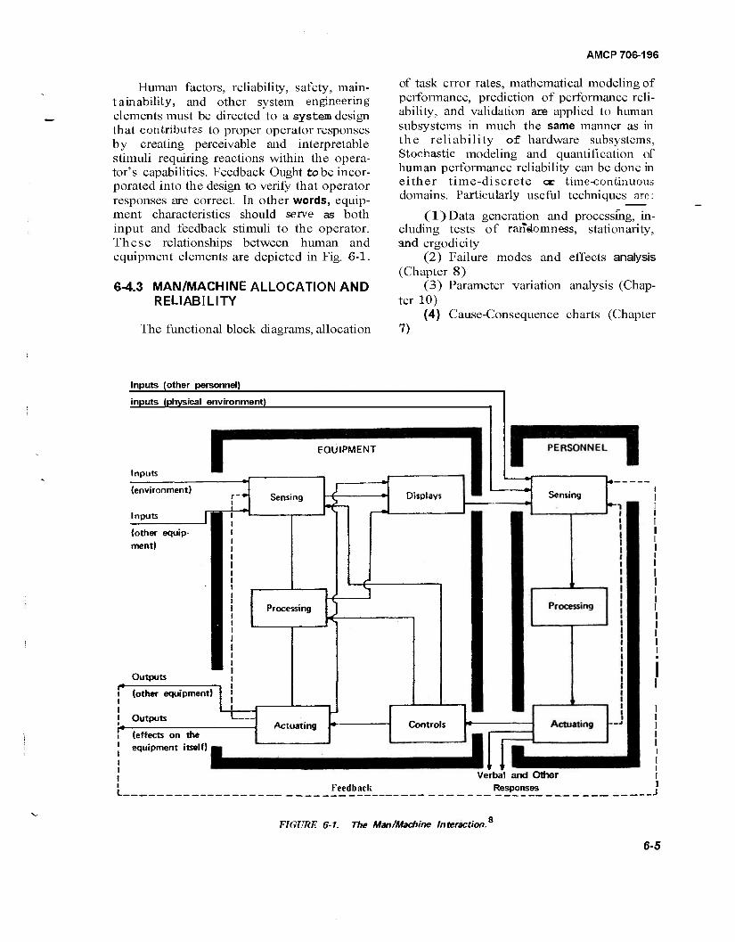
AMCP 706-196

Human factors, reliability, safety, maintainability, and other system engineering elements must be directed to a system design that contributes to proper operator responses by creating perceivable and interpretable stimuli requiring reactions within the operator's capabilities. Feedback Ought to be incorporated into the design to verify that operator responses are correct. In other words, equipment characteristics should serve as both input and feedback stimuli to the operator. These relationships between human and equipment elements are depicted in Fig. 6-1.

6-4.3 MAN/MACHINE ALLOCATION AND RELIABILITY

The functional block diagrams, allocation

of task error rates, mathematical modeling of performance, prediction of performance reliability, and validation are applied to human subsystems in much the same manner as in the reliability of hardware subsystems, Stochastic modeling and quantification of human performance reliability can be done in either time-discrete cur time-continuous domains. Particularly useful techniques are:

(l)Data generation and processing, including tests of randomness, stationarity, and ergodicity

(2) Failure modes and effects analysis (Chapter 8)

(3) Parameter variation analysis (Chap- ter 10)

(4) Cause-Consequence charts (Chapter 7)

Inputs (other personnel)

inputs (physical environment)

Inputs r EQUIPMENT

(environment)

Inputs

(other equipment)

Sensing £

Processing

Outputs

(other equipment)

Outputs TIZ

(effects on the equipment itself)

Displays

PERSONNEL

t 5

Actuating Controls

Sensing

Feedback

♦ t Verbal and Other

Responses

FIGURE 6-1. The Man/Machine Interaction. 8

6-5

AMCP 708-198

(5) Estimation of suitable distributions for random variables

(6) Decisionmaking methods such as hypothesis testing, multiple decision and sequential testing, and formulating rules for strategies.

Many of these techniques are discussed in greater detail in Refs. 25, 36-41,

Reliability cf asystem is affected by the allocation (not necessarily quantitative) of system functions to either the man, the machine, or both. Table 6-2 lists some of the salient characteristics of the humans and machines which are pertinent to the allocation choice. As is evident from studying Table 6-2, the prediction of human reliability is more difficult than the prediction of machine reliability. The machine's insensitivity to extraneous factors (Item 10 in Table 6-1) versus the human's sensitivity to these factors is one consideration, leading to human performance variability and the subsequent capability to predict machine reliability more precisely, hi fact, a human's response can be sufficiently influenced to vary from 0.0001 to 0.9999 reliability within conditions that would not affect a machine. The machine, for example, does not react to environments of combat which could produce severe psychological stress and breakdown in a human. Since the trade-off depends partly on the nature of the systan and human functions and partly on the way the allocation problem is approached, each design situation requires a separate human factors analysis, Such variables as cost, weight, size, hazard levels, adaptability, and state of technology must be considered for each system.

One approach to the choice between man and machine is to compare the predicted reliabilities of each. This approach, however, should not be based solely on failure rates, since humans are suffictenfly adaptable to recover quickly and correct some human- induced malfunctions. Similarly, humans have the flexibility to handle unique situations that might cause system failure if an unadaptable machine were assigned the task. An approach based on reliability conparisons ought to use failure rates in conjunction with an analysis of man/machine characteristics and the desired task accomplishments.

Another approach to man/machine allocation is illustrated by Fig. 6-2. This approach has three general steps:

(1) Develop a prediction model. (2) Generate Tääc Equipment Analysis

(TEA) data. (3) Predict man/machine reliability using

the TEA data as inputs to the prediction model.

The predictive model can be developed in either the time-discrete or time-continuous domains, depending on the nature of the human task. The human performance reliability is defined as (Ref. 42):

(l)Pr{task performance without error | stress}(discrete)

(2) Pr{task performance without error in an increment of time I stress} (continuous).

Embodied in the stress is the totality of all factors — psychological, physiological, and environmental—which affect human performance-

For discrete tasks such as pushing a but- ton or throwing a lever, 'the task random variable has only discrete values (often, the positive integers). The reliability of some discrete repetitive task (assuming that the trials are s-independent and have the Same probability) can be estimated simply as the fraction of the trials which are a success. The discrete human performance unreliability sometimes can be approximated by the error-rate multiplied by the time-interval (Raf ,24).

The time-continuous quantification of human perfonnance reliability is applied to such tasks as:

(1) Tracking a signal displayed on a Screen

(2) Manually controlling the pitch, roll, and yaw of an aircraft

(3) Performing a vigilance task which might require, for example, the detection of the presence (or absence) of a specified event. In this type of task, the random variable is continuous in time over some domain.

The time-to-error has a random distribution, just as time-to-failure of hardware; this distribution will have apdf, Cdf, Sf, and failure rate (enor rate). Depending on the specific task, a measure of human perfor-

6-6

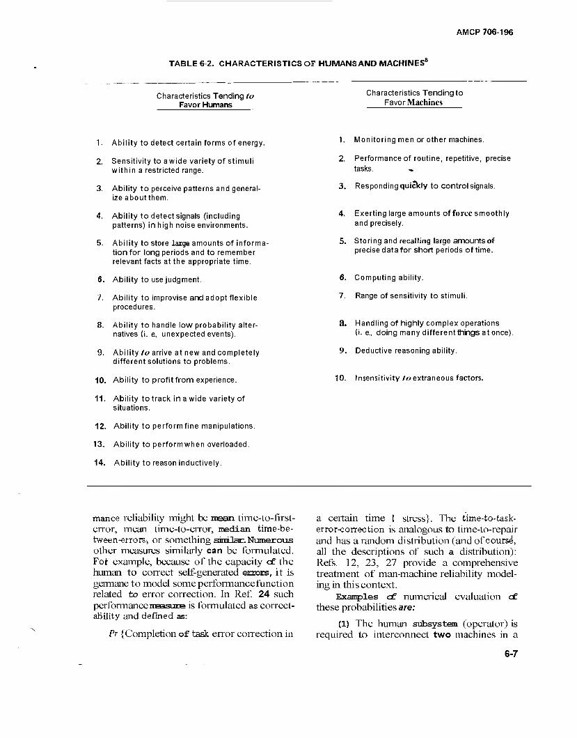
AMCP 706196

TABLE 6-2. CHARACTERISTICS OF HUMANS AND MACHINES8

Characteristics Tending to Favor Humans

Characteristics Tending to Favor Machines

1. Ability to detect certain forms of energy.

2. Sensitivity to a wide variety of stimuli within a restricted range.

3. Ability to perceive patterns and general- ize aboutthem.

4. Ability to detect signals (including patterns) in high noise environments.

5. Ability to store large amounts of information for long periods and to remember relevant facts at the appropriate time.

6. Ability to usejudgment.

7. Ability to improvise and adopt flexible procedures.

8. Ability to handle low probability alternatives (i. e, unexpected events).

9. Ability to arrive at new and completely different solutions to problems.

10. Ability to profit from experience.

11. Ability to track in a wide variety of situations.

12. Ability to perform fine manipulations.

13. Ability to performwhen overloaded.

14. Ability to reason inductively.

1. Monitoring men or other machines.

2. Performance of routine, repetitive, precise tasks. -

3. Responding quickly to control signals.

4. Exerting large amounts of force smoothly and precisely.

5. Storing and recalling large amountsof precise data for short periods of time.

6. Computing ability.

7. Range of sensitivity to stimuli.

3. Handling of highly complex operations (i. e., doing many differentthhgsat once).

9. Deductive reasoning ability.

10. Insensitivity to extraneous factors.

mance reliability might be mean time-to-first- error, mean time-to-error, median time-between-errorS) or something similar. Numerous other measures similarly can be formulated. For example, because of the capacity cf the human to correct self-generated errors, it is germane to model some performance function related to error correction. In Ref. 24 such performance measure is formulated as correctability and defined as:

Pr {Completion of task error correction in

a certain time I stress}. The time-to-task- error-correction is analogous to time-to-repair and has a random distribution (and of course, all the descriptions of such a distribution): Refs. 12, 23, 27 provide a comprehensive treatment of man-machine reliability modeling in this context.

Examples cf numerical evaluation cf these probabilities are:

(1) The human subsystem (operator) is required to interconnect two machines in a

6-7

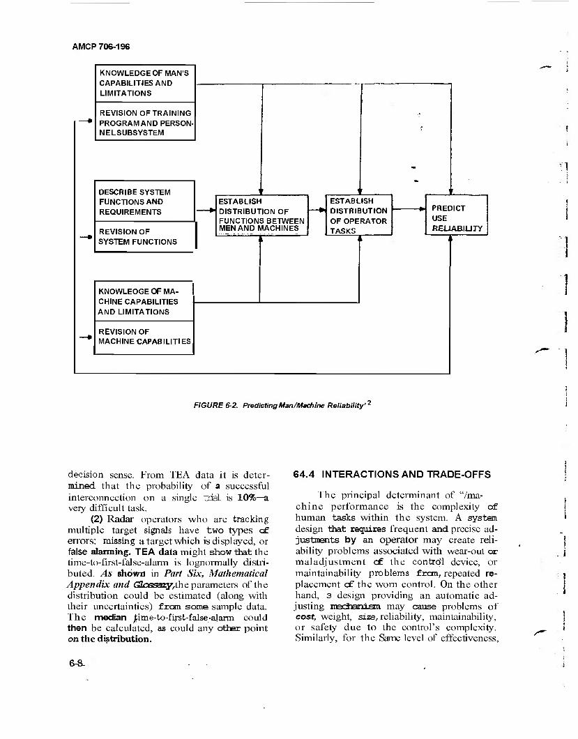
AMCP 706-196

KNOWLEDGE OF MAN'S CAPABILITIES AND LIMITATIONS

REVISION OF TRAINING PROGRAM AND PERSON- NELSUBSYSTEM

DESCRIBE SYSTEM FUNCTIONS AND REQUIREMENTS

REVISION OF SYSTEM FUNCTIONS

KNOWLEOGE OF MA- CHINE CAPABILITIES AND LIMITATIONS

ESTABLISH DISTRIBUTION OF FUNCTIONS BETWEEN MEN AND MACHINES

REVISION OF MACHINE CAPABILITIES

ESTABLISH DISTRIBUTION OF OPERATOR TASKS

PREDICT USE RELIABILITY

FIGURE 6-2. Predicting Man/Machine Reliability'

decision sense. From TEA data it is determined that the probability of a successful interconnection on a single trial is 10%—a very difficult task.

(2) Radar operators who are tracking multiple target signals have two types cf errors: missing a target which is displayed, or false alarming. TEA data might show that the time-to-first-false-alarm is lognormally distributed. As shown in Part Six, Mathematical Appendix and <3Zassary,the parameters of the distribution could be estimated (along with their uncertainties) from some sample data. The median jtime-to-first-false-alarm could then be calculated, as could any other point on the distribution.

64.4 INTERACTIONS AND TRADE-OFFS

The principal determinant of "/machine performance is the complexity of human tasks within the system. A system design that requires frequent and precise adjustments by an operator may create reliability problems associated with wear-out car maladjustment cf the control device, or maintainability problems from, repeated replacement cf the worn control. On the other hand, 3 design providing an automatic ad- justing mechanism may cause problems of cost, weight, size, reliability, maintainability, or safety due to the control's complexity. Similarly, for the Same level of effectiveness,

6-a.

AMCP 708-196

a system that through design, location, or environment is difficult to repair must necessarily be made more reliable than a system with a less complex man/machine interface. Thus, the man/machine interaction can contribute to, or detract frcm, the effectiveness of other disciplines depending upon trade- offs and interactions selected during the system engineering process.

Refs. 6, 18-21 give additional design guides and approaches for solving human factors problems and trade-offs with other disciplines. A valuable consideration, the use of human factors information by designers, is discussed and illustrated with tests and examples in Refs. 15-17.

6-4.5 THERP (TECHNIQUE FOR HUMAN ERROR RATE PREDICTION)

The human performance reliability model developed at Sandia Laboratories is defined as (Ref. 42):

"THERP is a method to predict human error rates and to evaluate the degradation to a man-machine system likely to be caused by human errors in association wLtin equipment functioning, operational procedures and practices, and other system and human characteristics which influence system behavior."

There are five steps in applying the model.

(1) Define the system failures (consequences). Work with the failures one at a time.

(2) List and analyze the human operations related to each failure (task analysis).

(3) Estimate the appropriate error probabilities.

(4) Estimate the effects of human errors on the system failure. Usually the hardware characteristics will have to be considered in the analysis.

(5) Recommend changes to the man/machine system and return to Step 2.

Ref. 42 summarizes and explains the THERP model (and extolls its virtues). Ref. 43 is an annotated bibliography of the Sandia Laboratories work in Irris area and will be

very helpful to anyone trying to estimate the effects of human frailty on a system. It lists 44 sources of further information.

REFERENCES

1. MIL-STD-1472, Human Engineering Design Criteria for Military Systems, Equipment and Facilities.

2. MIL-STD-803A-1, Human Engineering Design Critericrjor Aerospace Systems and Equipment, Part 1: Aerospace System Ground Equipment, 1964.

3. MIL-STD-803A-2, Humart Engineering Design Criteria for Aerospace Systems and Equipment, Part 2: Aerospace System Facilities and Facility Equip- ment, 1964.

4. MIL-STD-803A-3, Human Engineering Design Criteria for Aerospace Systems and Equipment, Part 3: Aerospace Ve- hicks and Vehicle Equipment, 1967.

5. MIL-H-46855, Human Engineering Re- quirements for Military Systems, Equip- men & and Facilities.

6. W. E. Woodson and D. W. Con over, Human Engineering Guide for Equip- ment Designers, Univ. of Calif Press, Berkeley, Calif, 1966.

7. MIL-STD-721, Definitions of Effective- ness Terms for Reliability, Maintain- ability, Human Factors, and Safety.

8. AR 70-8, Human Resources Research Program.

9. Anon., "Description of Human Factors Reports by Sandia Laboratories", July 1973, Available from Sandia Laborato- ries, Albuquerque, New Mexico 87115.

10. H. R. Leuba, "The Impact of Policy on Systan Reliability", IEEE Trans, on Reliability R-18, 137-140 (August 1969).

11. B. P. Davis and C. N. Cordoni, "People Subsystem Measurement for Total Reh5- ability", Proceedings of the 1970 An- nual Symposium on Reliability, 394 (1970).

12. G. E. Mller et al., Human Factors As- pects of Reliability, Publication No. U2296, Philco Corp., Newport Beach, Calif, 1964.

13. J. A Kraft, "Mtigation of Human Error through Human Factors Design Engi-

6-9

14.

15.

16.

AMCP 706-196 neering", Annals of 7äi Reliability and 26. Maintainability Conference 7, 300

(196B) . K. Inaba and R. Matson, "Measurement of Human Errors with Existing Data", Annals of 7th Reliability and Maintain- ability Conference!,301 (1968). D. Meister and D. E. Farr, The Utiliza- 27. tion of Human Factors Information by Designers, System Effectiveness Labora- tory, The Bunker-RamO Corp., Calif, 1967. 28.

D. Meister etäL, A Further Study of the Use of Human Factors Information by

Designers, System Effectiveness Labora- 29. tory, The Bunker-Ramo Corp., Calif, 1967. R W. Pew, Human Information-Proces- sing Concepts for System Engineers, 30. Univ. o/Michigan, Mich,, 1965. G. Chaikin et al., Engineering Practice Study-Human Engineering, Report No. RC-S-65-1, U S Army Mssile Com- mand, Redstone Arsenal, Ala, 1965. Davis, Faulkner, and Miller, "Work Physiology", Human Factors 11,No. 2, 157 (April 1969). Alan Swain, "The Human Element in System Development", Proceedings of the 1970 Annual Symposium on Reli- ability, 20-28 (1970). James J. Keenan, "Interactionist Models of the Varieties of Human Perfor- mance", Annals of 6th Reliability and 33. Maintainability Conference 6,76 (1967). D. Meister, "A Critical Review of Human Performance Reliability Predic- tive Methods", IEEE Trans. Reliability R-22, 116-123 (Aug. 1973). 34. D. Meister, "Comparative Analysis of Human Reliability Models", Final Re- port Contract N00024-71-C-1257, Bunk- er-Ramo Corp., Nov. 1971, AD-734 432. T. L. Regulinski and W. B. Askren, "Stochastic Modeling of Human Perfor- 35. mance Effectiveness Functions", Pro- ceedings 1972 Annual Reliability and Maintainability Symposium, 407-416 (1972). T. L. Regulinski, "Systems Maintain- ability Modeling", Proceedings 1970 36. Annual Reliability Symposium, 449-457 (1970).

17.

18.

19.

20.

21

22.

23.

24.

31.

32.

25.

T. L. Regulinski, "Quantification of Human Performance Reliability — Research Method Rationale", Proceed- ings of U S Navy Human Reliability Workshop, Report NAVSHIPS 0967-412-4010, Washington, D.C. (July 1971). T. L. Regulinski, Ed., Special Issue on Human Performance Reliability: IEEE Transactions on Reliability R-22, No. 3, August 1973. E. J. McCormis, Human Engineering, McGraw-Hill Publishing Co., New York, NY., 1967. D. Meister, "Human Factors in Reliabil- ity", Reliability Handbook, W. G. Ireson, Ed., McGraw-Hill Publishing Co., New York, NY, 1966. G. F. Rabideau, "Prediction of Person- nel Subsystem Reliability Early in Sys- tem Development Cycle", Proceedings of the National Aerospace System Reli- ability Symposium, institute of Aero- space Sciences, New York, NY., 1962. R. D. O'Connell, Handbook of Human Performance Measures, Space Biology Laboratory, yniveYsity of California, Los Angeles, July 1972. C. W. Simon, Economical Multifactor Designs for Human Factors Engineering Experiments; Hughes Aircraft Company Report No. HAC-P73-326, Culver City, Calif., June 1973. G. Chaikin, Human Factors/Human En- gineering; report of Ground Equipment and tfeterials Command, Army Mssile Command, Redstone Arsenal, Alabama, June 1973,AD-763 168. I. J. Little, The Design of Analysis of a Human Body Motion Measurement System; Report of Guidance and Con- trol Directorate, Army Missile Com- mand, Redstone Arsenal, Alabama, Sep- tember 1972, AD-751134. A. Chapanis, Relevance of Physiological and Psychological Criteria to Man-Ma- chine Systems—The Present State of the Art; Report TR-24, Dept. of Psychol- ogy, Johns Hopkins University, Md., 1970. T. L. Regulinski and W, B. Askren, Mathematical Modeling of Human Per- formance Errors for Reliability Analysis

1

6-10

of Systems, Report of Aerospace Medi- cal Research Laboratory No. AMRL- TR-68-93, Wright-Patterson AFB, Ohio 40. 45433, January 1969.

37. D. Meister et al., The Effect of Operator Performance Variables on Airborne Elec- tronic Equipment Reliability, Report 41. RADC-TR-70-140, Rome Air Develop- ment Center, Griffis AFB, N.Y., July 1970. * 42.

38. D. T. Hanifa, Human Perfoimance Quan- tification in System Deuelopment.Re- cent Advances, Report No. 70-M-0733 of Dunlap Associates, Inc., Santa Monica, Calif. July 1970.

39. A. I. Siegel and J. J. Wolf. Man-Machine

AMCP706 196

Simulation Models, John Wiley and Sons Publishing Co., New York, N.Y., 1969. A. I. Siegel and J. J. Wolf, "A Model for Digital Simulation of Two-Operator Man-Machine Systems", Ergonomics, 5:4 (1962). A. I. Siegel and J. J. Wolf, "A Technique for Evaluating Man-Machine Systems De- sign", Human Factors, 3:1 (1961). Alan D. Swain, "Shortcuts in Human Reliability Analysis", AM TO Advanced Study Institute on Generic Techniques in Systems 'Reliability Assessment, Nordhoff Publishing Company, Holland (1974, ±i press).

6-11

CHAPTER 7 CAUSE-CONSEQUENCE CHARTS

AMCP 706-196

7-1 INTRODUCTION

A Cause-Consequence chart shows the logical relationships between causes (events which are analyzed in no more detail) and consequences (events which are of concern only in themselves, not as they in turn affect other events). The chart usually is represented with consequences at the top and causes at the bottom; and the words Top and Bottom have come into common use to describe those portions cE the chart. A E&il- ure Modes and Effects Analysis (FMEA) deals largely with the bottom part of the chart. A fault tree is a part of a Cause-Con- sequence chart. It consists of only one consequence and all its associated branches. The remainder of this chapter deals mostly with fault trees. The Cause-Consequence chart is created by superimposing the separately created fault trees. The Cause-Consequence chart can be used to organize one's knowledge about any set of causes and their consequences; its use is not limited to hardware-oriented systems.

- The principles of fault tree creation are straightforward, and easy to grasp. The notation to be used and the discipline to be followed ought to be learned before trying to create a fault tree for a system. The practice of Fault Tree Analysis is tedious, extremely time consuming, and most profitable. Ordi- narily, it is done in conjunction with an FMEA (see Chapter 8) because both of the analyses deal with causes and consequences. The bookkeeping aspects—-viz., the keeping track of each item, its states (conditions) which are to be considered, and its place in the hierarchy-are very important because mistakes are so easy to make. Unless a strict discipline of labeling items and their states is followed, it is easy to make errors in identifying items, e.g., two different codes might be assigned to one item.

A fault tree usually is constructed in parts because it takes so much room. Each page of the fault tree refers to other pages of the fault tree and has certain conditions that are true for that page. One must carefully

keep track of all cf these in order to keep errors out of the fault tree.

There is a set ofconventions for constructing fault trees; it should be followed rig- orously. The reason for following the conven- tions is to have a fault tree whose parts can be created by several people and which can be understood by many" people, Since some set of rules must be followed, if utter chaos is to be avoided, one may as well choose the set in common use.

It is worthwhile keeping a file of general subtrees for common items (e.g., pumps and motors) to avoid having to create that subtree each time it is needed. In each application, the general subtree in the file can be pruned to fit the application.

Usually a fault tree is drawn with the same orientation as the Cause-Consequence chart: the trunk (representing the consequence) is at the top and the 'leaves (representing the causes) are at the bottom.

During the course of constructing the fault tree, there will be many false starts, blind alleys, system changes, and mistakes. The engineers will learn a great deal aboutthe system; in fact, this scheme of knowledge organization is useful precisely because it does require that the engineers know and make explicit assumptions about the relationships of items in the system.

Fault trees can be used for a complete plant as well as any of the component systems and subsystems. Fault trees provide an objective basis for analyzing system design, performing trade-off studies, analyzing common mode failures, demonstrating compliance with safety requirements, and justifying system changes or additions.

The logic of the approach makes it a visibility tool for both engineering and management. Many reliability techniques are inductive and are concerned primarily with assuring that hardware will accomplish reliably its assigned functions. The fault tree method is concerned with assuring that all critical aspects of a system are identified and control-

7-1

AMCP 706-196

led. The fault tree itself is a graphical representation of Boolean logic associated with the development of a particular systsn failure (consequence), called the TOP event; to basic failures (causes), called primary events. For example, the TOP event could be the failure of a reactor scram system to operate during an excursion, with the primary events being failures of the individual scram-system components.

In 1961 the concept of fault tree analysis was originated by Ball Telephone Labora- tories as a technique for safety evaluation of

^the MINUTEMAN Taunch Control System (Ref. l).At the 1965 Safety Symposium (Ref. 2) several papers expounded the virtues of fault tree analysis. They marked the beginning of a widespread interest in using fault tree analysis as a reliability tool in the nuclear reactor industry- In the early 1970's great strides were made in the solution of fault trees to obtain complete reliability informa- fcim about relatively complex systems (Refs. 3-7). The collection and evaluation of failure data are still very important (Refs. 8-11).

Fault tree analysis is of major value in:

1. Directing the analyst to ferret out failures deductively

2. Pointing out the aspects of a system which are important with respect to the failure of interest

3. Providing a graphical aid for system management people who are removed from the system design changes

4. Providing options for qualitative or quantitative system reliability analysis

5. Allowing the analyst to concentrate on one particular system failure at a time

6. Providing the analyst with genuine insight into system behavior.

Fault tree models do have disadvantages. Probably the most outstanding is the cost of development in first-time application to a system. As in the development of engineering drawings, the cost is somewhat offset by future application of the models in accident prevention, maintenance scheduling, and system modifications. The additional expense is justified by the detail resulting frcm fault tree analysis. Another disadvantage is that not many engineers are familiar with it. A lesser

disadvantage is that skilled personnel might develop a fault tree for a given system in different ways.

Although certain single failures that can result in several component failures simultaneously—called common mode failures*—can be pointed out by a detailed fault tree analysis, the analyst must be alert to include other common mode failures properly in the fault tree and to be aware that fault tree analysis does not inherently ferret out all common mode failures.

Most of this chapter is adapted from Ref. 17.

7-2 GENERATION

A system component is a basic acnstitu- ent for which failures are considered primary failures during fault tree construction. Conse- quently, the components of a given system can change depending on the TOP event being studied or the detail the analyst wishes to include in the fault tree analysis. Some components have several operating states, none of which are necessarily failed states. For example, relay contacts can be open or closed. The description of these states is called the component configuration.

Fault tree construction is the logical development of the TOP event. As the construction proceeds, each fault event also is developed until primary failures are reached. A fault event is a failure situation resulting from the logical interaction of primary failures. The development of any fault event lEsults in a brunch of the fault tree. The event being developed is called the base event of the branch. The branch is complete only when all events in the branch are developed to the level of primary failures. Every event in a branch is in the domain of the base event. In addition, if the base event is an input to an AND gate, every event in the branch is in the domain of every input to that AND gate.

A fault tree gate is composed of two parts:

1. The Boolean logic symbol that relates the inputs cf the gate to its output event

2. The output event description. •This nomenclature has been changed >" 1975 to "com-

mon cause" failure.

-]

7-2

AMCP 706-196

A gate is equivalent to another gate if and only if the logic symbol, the output event description, and the effective-boundary-conditions associated with the output event are identical. These effective-boundary conditions modify an event and are imposed by the analyst or are generated by previously occurring fault events, A complete treatment of these effective boundary conditions is given in Ref. 12. The event description must have two parts: (l)the incident identification, and (2) the entity identification. The incident identification defines, as briefly as possible, the fault without indicating any hardware involved. The entity identification specifies the item involved.

Two kinds of symbols are used in a fault tree: logic symbols as shown in Fig. 7-1, and event symbols as shown in Fig. 7-2 (Refs. 1,8,13,17).

The logic symbols (gates) are used to interconnect the events that contribute to the specified main (TOP) event. The logic gates that are used most frequently to develop fault trees are the basic AND and OR Boolean expressions. The AND gate provides an output event only if all input events occur simultaneously. The OR gate provides an output event if one or more of the input events are present.

The usual event symbols are the rectangle, circle, and diamond. The rectangle represents a fault event resulting from the combination cf more-basic faults acting through logic gates- The circle designates a basic system-component failure or fault input that is s-independent of all other events designated by circles and diamonds. The diamond symbol describes fault inputs that are considered basic in a given fault tree. However, the event is not basic in the sense that laboratory data are applicable. Rather, the fault tree is simply not developed further, either because the event is of insufficient consequence or the necessary information is unavailable. In order to solve a fault tree, both circles and diamonds must be used to represent events for which reliability information is necessary to the fault tree. Events that appear as circles or diamonds are treated as primary events.

The triangles shown in Fig- 7-2 strictly

are not event-symbols although traditionally theyâve been classified as such. The triangle indicates a transfer from one part of the fault tree ■> another'. A line from the side of the trianjie (transfer-out triangle) denotes an evenfcr transfer out from the associated logic gate. A line from the apex of the triangle denotes an event transfer info the a^sorint^d logic gate frcm the transfer-out triangle with the Same identification-number.

The other logic gates and events symbols are shown and explained in Figs. 7-1 and 7-2.

A minimal cut set is a smallest set of primary events, inhibit conditions, and/or undeveloped fault events which must all occur in order for the TOP event to occur. The primary events represent the resolution of the fault tree. The minimal cut sets represent the modes by which the TOP event can occur. For example, the minimal cut set A, A, means that both the primary events A, and A, must occur in order for the TOP event to occur. The occurrence of A, and A, is a mode by which the TOP event occurs. If either A, or A, doe3 not'occur, then the TOP event does not occur by this mode. The set of events A, A2C, where C is another primary event, is not a rniraiial cut set because C is redundant and is not necessary for the occurrence of the TOP event; C can either occur or not occur, and as long as A, and A both occur, then the TOP event will occur. A minimal cut set is a collection of component failures all of which are necessary and sufficient to cause systaem failure by that irdmrral cut set. A complete set of minimal cut sets is all the failure modes for the given system-failure.

The minimal cut sets are important because they depict which failures must be repaired in order for the TOP failure to be removed from the failed state. The minimal cut sets point out the weakest links in the sysban. The primary events in the 1-event minimal cut sets usually are the most important, A 1-failure analysis is a fault tree drawn to obtain only the 1-event minimal cut sets (1-failure) for the TOP event. For a 1-failure

analysis, the fault tree ends whenever an AND gate is reached that does not have deeper common causes (which effectively transform an AND gate to an OR gate),

7-3

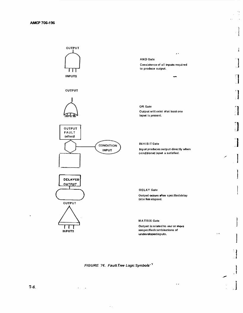
AMCP 706-196

OUTPUT

AND Gate

Coexistence of all inputs required to produce output.

OUTPUT

OR Gate

Output will exist if at least one input is present.

OUTPUT FAULT (effect)

DELAYEO

OUTPUT

CD OUTPUT

TTT INPUTS

INHIBITGate

Input produces output directly when conditional input is satisfied.

OELAY Gate

Output occurs after specified delay time has elapsed.

MATRIX Gate

Output is related to one or more unspecified combinations of undeveloped in p uts.

FIGURE 7-/. Fault Tree Logic Symbols'''

7-4

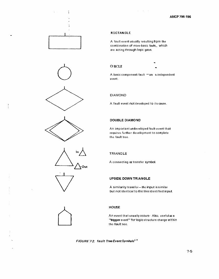
AMCP 706-196

RECTANGLE

A fault event usually resulting frpm the

combination of more-basic faults,, which

are acting through logic gates.

Cl RCLE

A basic component-fault — an s-independent

event.

-Out

DIAMOND

A fault event not developed to its cause.

DOUBLE DIAMOND

An important undeveloped fault-event that

requires further development to complete

the fault tree.

TRIANGLE

A connecting a: transfer symbol.

UPSIDE DOWN TRIANGLE

A similarity transfer— the input is similar

but not identical tothe like identified input.

HOUSE

An event that usually occurs- Also, useful as a

"triggerevent" for logicstructure change within

the fault tree.

FIGURE 7-2. fault Tree Event Symbols*

7-5

AMCP 706-196

Fault trees are very flexible with regard to the degree of detail to be included. In the fault tree itself primary failures can be failures of the smallest mechanical linkage in a micro- switch or failures of a power-generating station. The resolution of the analysis is determined by the needs of the analyst. Having determined the resolution, the analyst has options with regard to evaluating the fault tree. Indeed, the fault tree itself can be the final objective. In addition to the system visibility and understanding obtained by studying the fault tree, further qualitative analysis of the fault tree can produce all of thesystem modes of failure. Finally quantitative evaluation is possible, i.e., probabilistic failure information can be obtained about the TOP event and minimal cut sets from probabilistic failure information about the components.

Generation of fault trees has two steps: system definition and construction of the tree. Each step is discussed in the paragraphs that follow.

7-2.1 SYSTEM DEFINITION

System definition is often the most difficult task associated with fault tree analysis. Of primary importance is a functional layout diagram of the system showing all functional interconnections and identifying each system component. (For some systems that are not hardware oriented, such a diagram may not exist and, indeed, the Cause-Consequence chart itself might be the only feasible dia- grammatic system representation.) An example might be a detailed electrical schematic. Physical syyltm. bounds are then established to focus the attention of the analyst on the precise area cf interest. A common error is failure to establish realistic system bounds and thereby to initiate a diverging analysis.

Sufficient information must be available for each of the system components to allow the analyst to determine the necessary modes of failure of the 'components. This information can come from the experience of the analyst or from the technical specifications of the components,

Next, the system boundary conditions must be established. These boundary conditions are not to be confused with the physical

7-6-

bounds of the system. System boundary conditions define the situation for which the fault tree is to be drawn. A most important system boundary condition is the TOP event. For any given system, there; is a multitude of possibilities for TOP events. Selecting an appropriate TOP event is sometimes difficult. The complete Cause-Consequence chart will have many TOP events. One of them is chosen for each fault tree. Chousing good, useful TOP events is not easy because one is rarely sure how high to go. The system initial configuration is described by additional system boundary conditions. This configuration must represent the system in the unfailed state. Consequently, these system boundary conditions depend on the TOP event. Initial conditions are then system boundary conditions that define the component configurations for which the TOP event is applicable. All components that have more than one operating state generate an initial condition. System boundary conditions also include any fault event declared to exist or to be not-allowed for the duration of the fault tree construction. These events are called existing system boundary conditions or not-allowed system boundary conditions. An existing system boundary condition is treated as certain to occur, and a not-allowed system boundary condition is treated as an event with no possibility of occurring. Neither existing nor not-allowed system boundary conditions appear as events in the final system fault tree. Finally, in certain cases, partial development of the TOP event, called the treetop, also is required as a system boundary condition. If the treetop system boundary condition is required, it is not considered as part of the fault tree construction process because it is obtained by inductive means.

7-22 FAULT TREE CONSTRUCTION

Published information dealing with generalized fault tree construction is quite limited. Haasl (Ref. l)ias described some general concepts, and Fussell (Ref. 12) has presented a construction methodology for electrical systems that is deductive and formal,

An example demonstrates some of the fundamental aspects of fault tree construction. A sample system schematic is shown in

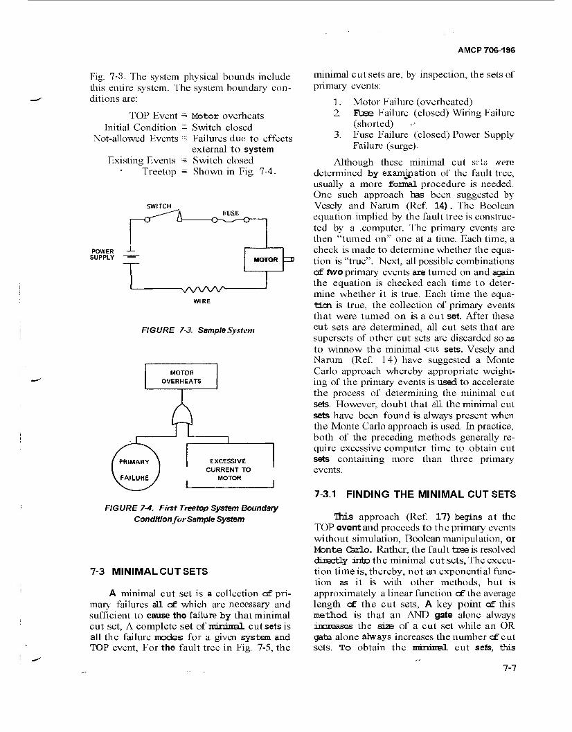
AMCP 706-196

Fig. 7-3. The system physical bounds include this entire system. The system boundary conditions are:

TOP Event = Motor overheats Initial Condition =

Not-allowed Events ~

Existing Events = Treetop =

SWITCH

POWER -x- SUPPLY -=~

Switch closed Failures due to effects external to system Switch closed Shown in Fig. 7-4.

FUSE

T MOTOR ZD

\AAAAA WIRE

FIGURE 7-3. Sample System

MOTOR OVERHEATS

I PRIMARY \

^FAILURE J L

EXCESSIVE CURRENT TO

MOTOR J

FIGURE 7-4. First Treetop System Boundary Condition for Sample System

7-3 MINIMAL CUT SETS

A minimal cut set is a collection of primary failures all of which are necessary and sufficient to cause the failure by that minimal cut set, A complete set of imrairal cut sets is all the failure modes for a given system and TOP event, For the fault tree in Fig. 7-5, the

minimal cut sets are, by inspection, the sets of primary events:

1. Motor Failure (overheated) 2. Rjse Failure (closed) Wiring Failure

(shorted) 3. Fuse Failure (closed) Power Supply

Failure (surge).

Although these minimal cut sets .vere determined by examination of the fault tree, usually a more formal procedure is needed. One such approach has been suggested by Vesely and Narum (Ref. 14). The Boolean equation implied by the fault tree is constructed by a .computer. The primary events are then "turned on" one at a time. Each time, a check is made to determine whether the equation is "true". Next, all possible combinations of two primary events are turned on and again the equation is checked each time to determine whether it is true. Each time the equation is true, the collection of primary events that were turned on is a cut set. After these cut sets are determined, all cut sets that are supersets of other cut sets are discarded so as to winnow the minimal -cut sets. Vesely and Narum (Ref. 14) have suggested a Monte Carlo approach whereby appropriate weighting of the primary events is used to accelerate the process of determining the minimal cut sets. However, doubt that all the minimal cut sets have been found is always present when the Monte Carlo approach is used. In practice, both of the preceding methods generally require excessive computer time to obtain cut sets containing more than three primary events.

7-3.1 FINDING THE MINIMAL CUT SETS

This approach (Ref. 17) begins at the TOP event and proceeds to the primary events without simulation, Boolean manipulation, or Monte Carlo. Rather, the fault tree is resolved directly into the minimal cut sets, The execu- tion time is, thereby, not an exponential function as it is with other methods, but is approximately a linear function cf the average length of the cut sets, A key point cf this method is that an AND gate alone always increases the size of a cut set while an OR gate alone always increases the number cf cut sets. To obtain the rmrriiral cut sets, this

7-7

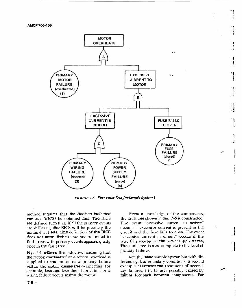
AMCP 706-196

EXCESSIVE CURRENT TO

MOTOR

EXCESSIVE CUR RENT IN

CIRCUIT FUSE FAILS

TO OPEN

FIGURE 7-5. First Fault Tree forSample System 1

method requires that the Boolean indicated cut sets (BICS) be obtained fust. The BICS are defined such that, if all the primary events are different, the BICS will be precisely the minimal cut sets. This definition of the BICS does not mean tinefc the method is limited to fault trees with primary events appearing only once in the fault tree.

Fig. 7-4 TPfioM-g the inductive reasoning that the motor overheats if an electrical over! oad is supplied to the motor or a primary failure within the motor causes the overheating; for example, bearings lose their lubrication or a wiring failure occurs within the motor.

From a knowledge of the components, the fault tree shown in Ekr. 7-5 is constructed. The event "excessive current to motor" occurs if excessive current is present in the circuit and the fuse fails to open. The event "excessive current in circuit" occurs if the wire fails shorted or the power supply surges, The fault tree is now complete to the level of primary failures.

For the same sample system but with different system boundary conditions, a second example illastiatBS the treatment of secondary failures, i.e., failures possibly caused by failum feedback between components. For

7-8 --

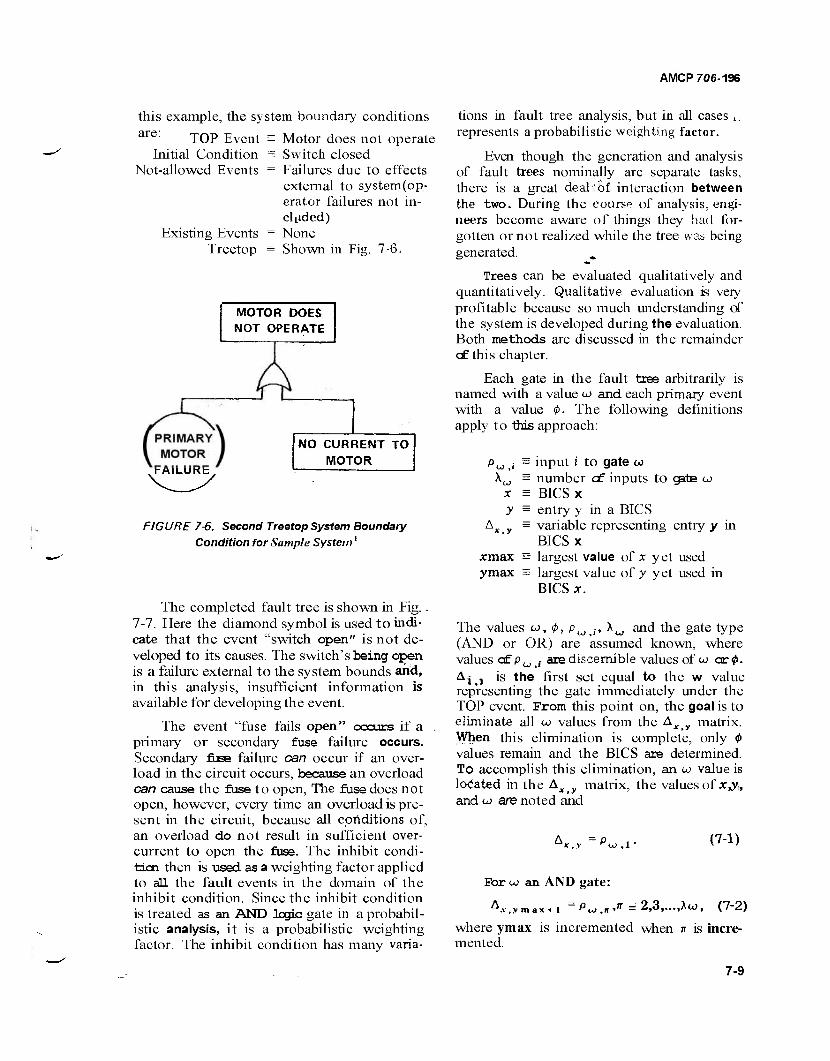
AMCP 706-196

this example, the system boundary conditions

TOP Event = Motor does not operate are:

Initial Condition Not-allowed Events

Existing Events Treetop

Switch closed Failures due to effects external to system (operator failures not included) None Shown in Fig. 7-6-

MOTOR DOES NOT OPERATE

PRIMARY MOTOR

'FAILURE.

NO CURRENT TO MOTOR

FIGURE 7-6. Second Treetop System Boundary Condition for Sample System'

The completed fault tree is shown in Fig.. 7-7. Here the diamond symbol is used to indicate that the event "switch open" is not developed to its causes. The switch's being open is a failure external to the system bounds and, in this analysis, insufficient information is available for developing the event.

The event "fuse fails open" occurs if a primary or secondary fuse failure occurs. Secondary fuse failure can occur if an overload in the circuit occurs, because an overload can cause the fuse to open, The fuse does not open, however, every time an overload is present in the circuit, because all conditions of, an overload do not result in sufficient over- current to open the fuse. The inhibit condition then is used as a weighting factor applied to all the fault events in the domain of the inhibit condition. Since the inhibit condition is treated as an AND logic gate in a probabilistic analysis, it is a probabilistic weighting factor. The inhibit condition has many varia-

tions in fault tree analysis, but in all cases t. represents a probabilistic weighting factor.

Even though the generation and analysis of fault trees nominally are separate tasks, there is a great deal "of interaction between the two. During the course of analysis, engineers become aware of things they had forgotten or not realized while the tree was being generated.

Trees can be evaluated qualitatively and quantitatively. Qualitative evaluation is very profitable because so much understanding of the system is developed during the evaluation. Both methods are discussed in the remainder cf this chapter.

Each gate in the fault tree arbitrarily is named with a value to and each primary event with a value <P- The following definitions apply to this approach:

PU|j = input i to gate w XJJ = number cf inputs to gate to

x = BICS x y = entry y in a BICS

Ax y = variable representing entry y in BICS x

jcmax = largest value of x yet used ymax = largest value of y yet used in

BICS x.

The values to, 4>, P^j, Xw and the gate type (AND or OR) are assumed known, where values ofpUi/ are discernible values of to or 0. 4jj is the first set equal to the w value representing the gate immediately under the TOP event. From this point on, the goal is to eliminate all to values from the A matrix. When this elimination is complete, only <t> values remain and the BICS are determined. To accomplish this elimination, an to value is located in the Axy matrix, the values of xy,, and to are noted and

'w.i- (7-1)

For tu an AND gate:

A.r.vraax + 1 = P^ ,n >n = 2,3,...,Aw, (7-2)

where ymax is incremented when n is incremented.

7-9

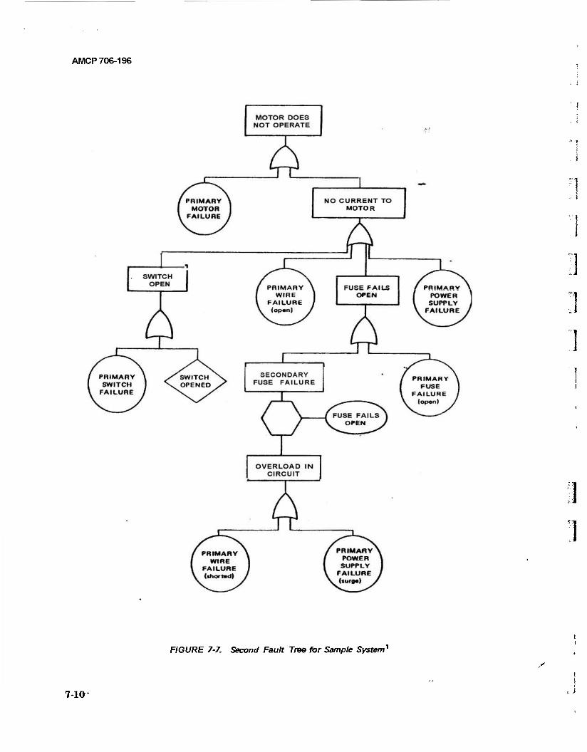
AMCP 706-196

' I

FIGURE 7-7. Second Fault Tree for Sample System'1

710"

AMCP 706-196

For w an OR gate:

Ax „, n = l,2,...,ymax; n # y x m a x + 1 ,n r» a -v

P^.ny n = 2,3,-,^ ,n = y (7-3)

where xmax is incremented when JT is incremented.

Eqs. 7-1 and 7-2 or 7-3 are repeated until all the entries in the Ax y matrix become values of <p. The BICS are then determined. A simple search procedure is used to determine the mirrimal cut sets.

The number of BICS (the number of rows in the Axy matrix) for a fault tree generally can be determined in areasonable time by hand. The number of BICS is an upper bound to the number of minimal cut sets. If xij is a parameter associated with input j to gate i, where xLt = 1 for ail primary events, then

X: X, if i is an'ÄNÖ'gate

if i is an OR gate

Xk,K ~ X{

X. ijm ax' (7-4)

+ JC ijmax»(7_5)

(7-6)

where k is the gate into which Gate i is input £. If logic gate i is directly under the TOP event then Xt = XTOP is the number of BICS for the fault tree. The value xk is determined only when all its input parameters are determined; henoe, gates that have only primary events (x, j = 1 for all;') as input are the beginning points.

The computation is simple, as can be seen from examining the fault tree in Fig. 7-5. From Bq. 7-5, Xc = (1 + 1) = 2 and then from Bq. 7-4,

XB = (*B !>(*„ 2) - (Xc)(xB 2) = (2)(1) = 2 (7-7)

and, finally, since A is an OR gate

XA = XroP = (XA j ) + (XA 2 ) = (XA ,1 )

+ XB =3 . (7-8) Therefore, the Ax y iratrxx cxntains three

rows. The maximum number of primary events in any BICS for a fault tcee also generally can be determined in a reasonable time

by hand. This maximum is an upper bound to the maximum number cf primary events in any minimal cut set for that fault tree. The determination is similar to that for the number of BICS. If ytj is aparameter associated with input j to gate r'where ytJ = 1 for all primary events, then

y,M + yt.t + yt,3 +■ Y _ if / is an AND^gate

max {yi.i,yt,2>yi.3, if i is an OR gate

+ 3iJr

(7-9)

rfe.fi = V.

***' îjm ax J » (7-10)

(7-11)

where k is the gate into which Gate i is input $.. If logic gate i is directly under the TOP event, then Y. = YTOP is the maximum number af primary events in any BICS for the given fault tree. Yi is determined only when all its input parameters are determined; hence, the analyst must begin with gates that have only primary events (y, y = 1 for all ;') as input.

For example, the fault tree in Fig. 7-5 is again considered. From Eq. 7-10, Yc = max (1,1} = land from Eq. 7-9,

YB = Yc + y B,2 (7-12)

YA = YTOP = max {!'2J =2-

Therefore, the largest BICS contains two primary events. The Ax matrix for the fault tree of Fig. 7-5 is a 2 X 3 matrix. This method easily can be extended to determine the maximum number of 1-, 2-, 3-, ... event BICS, hence an upper bound on the 1-, 2-, 3-, ... event minimal cut sets, respectively, is determined.

The fault tree of Fig. 7-5 illustrates the method cf determining minimal cut sets. Each gate has been labeled with a letter and each., primary event with a number. The input is then

03 Gate Type yw 'u>A

A OR 2 1 B B AND 2 c 2 C OR 2 4 3

7-11

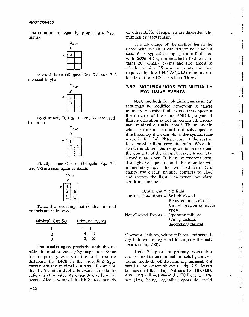
AMCP 708-198

The solution is begun by preparing a Afc y

matrix: A*.y

Y

x A

Since A is an OR gate, Eqs. 7-1 and 7-3 are used to give

A, „

1 B

To eliminate B, Eqs. 7-1 and 7-2 are used to obtain

A, „

1 C 2

Finally, since C is an OR gate, Eqs. 7-1 and 7-3 are used again to cbtain

1

3 2

From the preceding matrix, the minimal cut sets are as follows:

KfrmitBl Cut Set

1 2 3

Primary Events

1 4, 2 3, 2

The results agree precisely with the results obtained previously by inspection. Since all the primary events in the fault tree are different, the BICS in the preceding Ax y

matrix are the minimal cut sets. If some of the BICS contain duplicate events, this dupli- cation is eliminated by discarding redundant events. Also,if some of the BICS are supersets

of other BICS, all supersets are discarded. The minimal cut sets remain.

The advantage of the method lies in the speed with which it can determine large cut sets, As a typical example;, for a fault tree with 2000 BICS, the smallest of which contains 20 primary events and the largest of which contains 25 primary events, the time required by the UNIVACJ.108 computer to locate all the BICS is less than 16sec,

7-3.2 MODIFICATIONS FOR MUTUALLY EXCLUSIVE EVENTS

Mast methods for obtaining rrdrrirral cut sets must be modified somewhat to handle mutually exclusive fault events that appear in the domain of the same AND logic gate. If this modification is not implemented, erroneous "minimal cut sets" result. The manner in which erroneous rmrrirnal cut sets appear is illustrated by the example in the system schematic in Fig. 7-8. The purpose of the system is to provide light from the bulb. When the switch is closed, the relay contacts close and the contacts of the circuit breaker, anormally closed relay, open. If the relay contacts open, the light will go out and the operator will immediately open the switch which in turn causes the circuit breaker contacts to close and restore the light. The system boundary conditions include:

TOP Event = No light Initial Conditions = Switch closed

Relay contacts closed Circuit breaker contacts open

Not-allowed Events = Operator failures Wiring failures Secondary failures.

Operator failures, wiring failures, and secondary failures are neglected to simplify the fault tree (seeFig. 7-9).

Table 7-1 gives the primary events that are declared to be minimal cut sets by conventional methods of determining imimral cut sets for the system shown in Eg. 7-8, As can be reasoned Atom Fig. 7-8,sets (6), (8), (10), and (12) will not cause the TOP event. Only set (12), being logically impossible, could

•

7-13

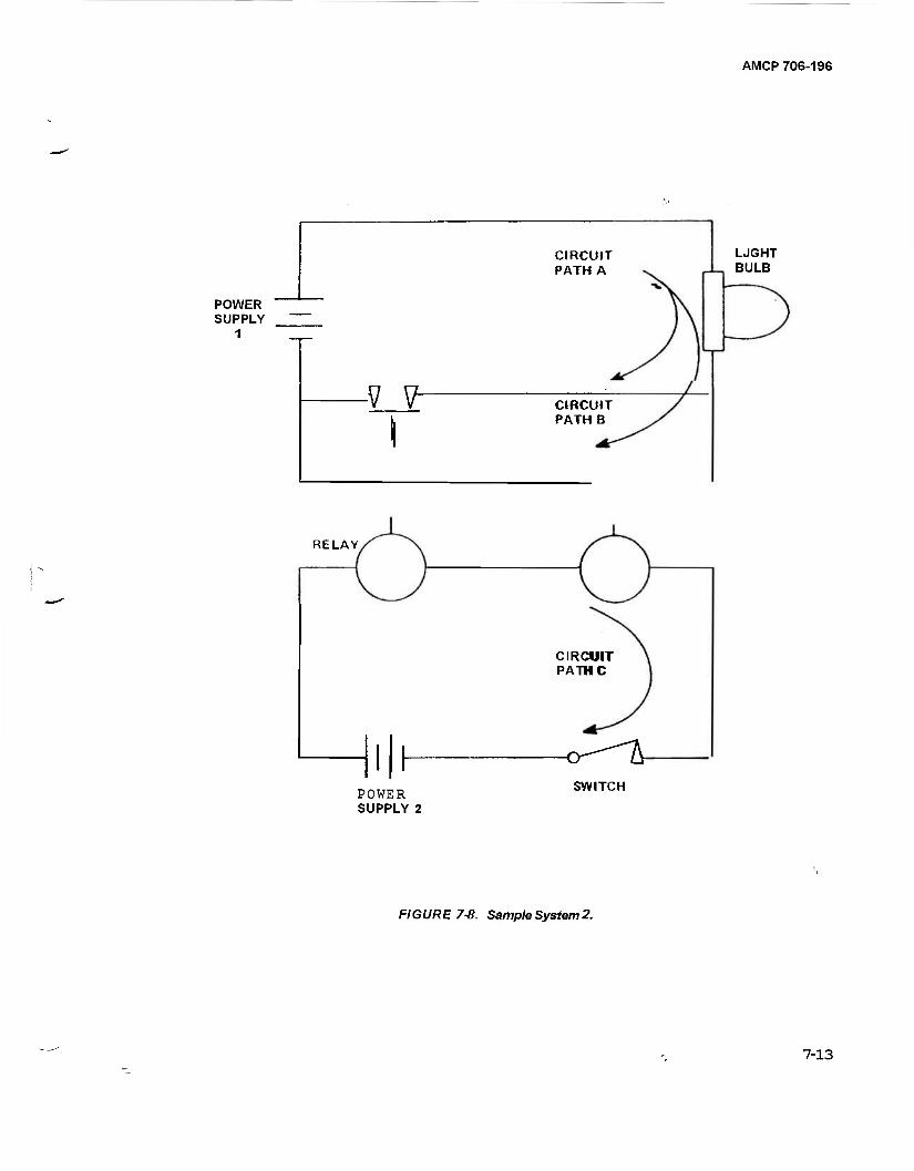
AMCP 706-196

CIRCUIT PATH A

LJGHT BULB

POWER SUPPLY

1

-v v- I

CIRCUIT PATH B

RELAY

CIRCUIT PATHC

■o-"-"k POWER SUPPLY 2

SWITCH

FIGURE 7-6. Sample System 2.

7-13

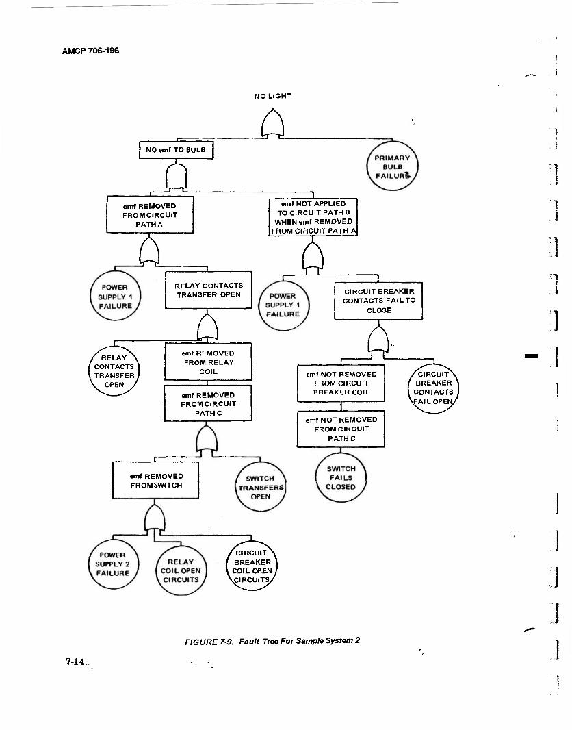
AMCP 706-196

NO LIGHT

a NO emf TO BULB

2 emf REMOVED FROM CIRCUIT

PATH A

1 emf NOT APPLIED

TO CIRCUIT PATH B

WHEN emf REMOVED FROM CIRCUIT PATH A

RELAY CONTACTS TRANSFER OPEN

~\

CIRCUIT BREAKER CONTACTS FAIL TO

CLOSE

RELAY CONTACTS TRANSFER

OPEN

emf REMOVED FROM RELAY

COIL

X emf REMOVED FROMCIRCUIT

PATHC

X emf NOT REMOVED

FROM CIRCUIT BREAKER COIL

'CIRCUIT^ BREAKER

CONTACTS

^FAILOPEN/

emfNOT REMOVED FROMCIRCUIT

PATH C

emf REMOVED FROM SWITCH

CIRCUIT BREAKER

COIL OFEN ;

^CIRCUITS/

FIGURE 7-9. Fault Tree For Sample System 2

7-14,

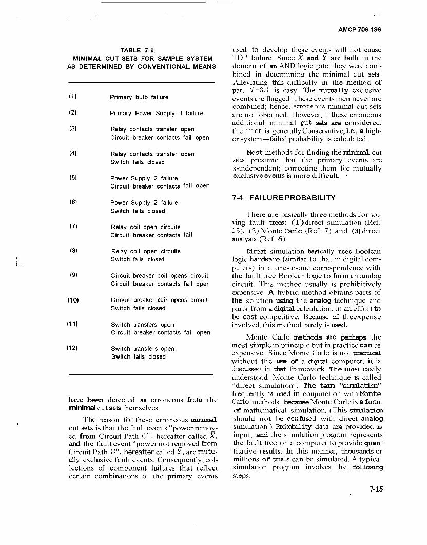
AMCP 706-196

TABLE 7-1. MINIMAL CUT SETS FOR SAMPLE SYSTEM

AS DETERMINED BY CONVENTIONAL MEANS

(1) Primary bulb failure

(2) Primary Power Supply 1 failure

(3) Relay contacts transfer open Circuit breaker contacts fail open

(4) Relay contacts transfer open Switch fails closed

(5) Power Supply 2 failure Circuit breaker contacts fail open

(6) Power Supply 2 failure Switch fails closed

(7) Relay coil open circuits Circuit breaker contacts fail

(8) Relay coil open circuits Switch fails closed

<9) Circuit breaker coil opens circuit Circuit breaker contacts fail open

(10) Circuit breaker coil opens circuit Switch fails closed

(11) Switch transfers open Circuit breaker contacts fail open

(12) Switch transfers open Switch fails closed

have been detected as erroneous from the minimal cut sets themselves.

The reason for these erroneous mmimal cut sets is that the fault events "power removed from Circuit Path C", hereafter called X, and the fault event "power not removed from Circuit Path C", hereafter called Y, are mutually exclusive fault events. Consequently, col- lections of component failures that reflect certain combinations of the primary events

used to develop the_se events will not cause TOP failure. Since X and Y are both in the domain of an AND logic gate, they were combined in determining the minimal cut sets. Alleviating this difficulty in the method of par. 7—3.1 is easy. The mutually exclusive events are flagged. These events then never are combined; hence, erroneous minimal cut sets are not obtained. However, if these erroneous additional minimal .cut sets are considered, the error is generally Conservative; i.e., a higher system—failed probability is calculated.

Most methods for finding the minimal cut sets presume that the primary events are s-independent; correcting them for mutually exclusive events is more difficult. -

7-4 FAILURE PROBABILITY

There are basically three methods for solving fault trees: (1)direct simulation (Ref. 15), (2) Monte Carlo (Ref. 7), and (3) direct analysis (Ref. 6).

Direct simulation basically uses Boolean logic hardware (similar to that in digital computers) in a one-to-one correspondence with the fault tree Boolean logic to form an analog circuit. This method usually is prohibitively expensive. A hybrid method obtains parts of the solution using the analog technique and parts from a digital calculation, in an effort to be cost competitive. Because of theexpense involved, this method rarely is used.

Monte Carlo methods are perhaps the most simple in principle but in practice can be expensive. Since Monte Carlo is not practical without the use of a digital computer, it is discussed in that framework. The most easily understood Monte Carlo technique is called "direct simulation". The term "sirtulaticn" frequently is used in conjunction with Monte Carlo methods, because Monte Carlo is a form? cE mathematical simulation. (This simulation should not be confused with direct analog simulation.) Rrohahi 1 ity data are provided as input, and the simulation program represents the fault tree on a computer to provide quantitative results. In this manner, thousands or millions of trials can be simulated. A typical simulation program involves the following steps.

7-15

AMCP 706-1 96

1. Assign failure data to input fault events within the tree and, if desired, repair data.

2. Represent the fault tree on a computer to provide quantitative results for the overall system performance, subsystem performance, and the basic input event performance.

3. List the failure that leads to the undesired event and identify minimal cut sets contributing to the failure.

4. Compute and rank basic input failure and availability performance results.

In performing these steps, the computer program simulates the fault tree and, using the input data, randomly selects the various parameter data from assigned statistical distributions; and then tests whether or not the TOP event occurred within the specified time period, Each test is a trial, and a sufficient number of trials is run to obtain the desired quantitative resolution, Each time the TOP event occurs, the contributing effects of input events and the logical gates causing the specified TOP event are stored and listed as computer output, The output provides a detailed perspective of the system under simulated operating conditions and provides a quantitative basis to support objective decisions.

To illustrate how direct analysis might be applied to a simple fault tree for static conditions, the fault tree shown in Fig. 7-10 is considered, It contains s-independent, primary events A, B, C, and D with constant probabilities of 'failure 0.1, 0.2, 0.3, and 0.4, respectively, This assumption of constant failure probabilities distinguishes this example from realistic fault tree evaluation. The fault tree, as shown in Fig, 7-10, is not in convenient form because Events XI and X2 are not s-independent—they both are functions of Primary Event B. By Boolean manipulation the fault tree shown in Fig. 7-11 is equivalent to the one shown in Fig. 7-10; the minimal cut sets for both fault trees are identical, The fault tree shown in Fig. 7-11 is in convenient form for calculating the probability of the TOP event.

Two basic laws of probability are used in a fault tree evaluation,

7-16

FIGURE 7-10. Sample Fault Tree for

Probability Evaluation.

Pr{AluA2} = Pr{Al}+Pr{A2}- Pr{AinA2} (7-14)

Pr{AlnA2} = Pr{Al) Pr{A2\Al] (7-15)

where

A I, A 2 = any two events u = logic symbol for union, and/or

(often represented as addition) n = logic symbol for intersection,

both/and (often represented as mul- tiplication)

Eq. 7-14 simply states that the probability of a union is the sun of the probabilities of the individual events minus the probability of their intersection. In terms of the fault tree, the probability of a 2-event OR gate is the sum of probabilities of the two events attached to the gate minus the probability of the two events both occurring. Eq. 7-15 states that the probability of an intersection is the probability of one, Pr {Al}, times the probability of the other, given the occurrence of the first, Pr {A2\A1} , In terms of the fault tree in Fig. 7-11, the probability of a 2-event AND gate is the product of the probabilities of the two attached events, because primary events of a fault free are s-independent; (if not, special precautions must be taken as mentioned in par. 7-3.2).

:I

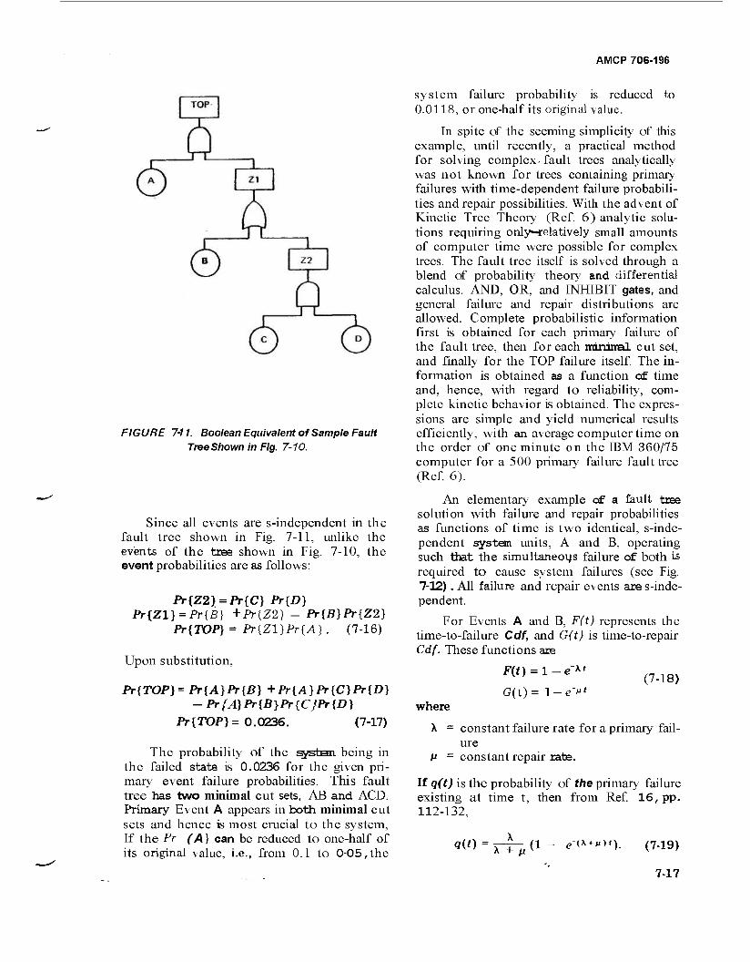
AMCP 706-196

FIGURE 7-11. Boolean Equivalent of Sample Fault Tree Shown in Fig. 7-10.

Since all events are s-independent in the fault tree shown in Fig. 7-11, unlike the events of the tree shown in Fig. 7-10, the event probabilities are as follows:

Pr{Z2} = Pr{C] Pr{D} Pr{Zl) = Pr{B} + Pr{Z2] - Pr{B)Pr{Z2}

Pr{TOP}= Pr{Zl}Pr{A] . (7-16)

Upon substitution,

Pr{TOP}= Pr{A}Pr{B} + Pr{A] Pr{C}Pr{D} - Pr{A}Pr{B}Pr{C}Pr{D}

Pr {TOP} =0.0236. (7-17)

The probability of the systsn being in the failed state is 0.0236 for the given primary event failure probabilities. This fault tree has two minimal cut sets, AB and ACD. Primary Event A appears in both minimal cut sets and hence is most crucial to the system, If the Pr (A) can be reduced to one-half of its original value, i.e., from 0.1 to 0-05,the

system failure probability is reduced to 0.0118, or one-half its original value.

In spite of the seeming simplicity of this example, until recently, a practical method for solving complex, fault trees analytically was not known for trees containing primary failures with time-dependent failure probabilities and repair possibilities. With the advent of Kinetic Tree Theory (Ref. 6) analytic solutions requiring only—relatively small amounts of computer time were possible for complex trees. The fault tree itself is solved through a blend of probability theory and differential calculus. AND, OR, and INHIBIT gates, and general failure and repair distributions are allowed. Complete probabilistic information first is obtained for each primary failure of the fault tree, then for each minimal cut set, and finally for the TOP failure itself. The information is obtained as a function of time and, hence, with regard to reliability, complete kinetic behavior is obtained. The expressions are simple and yield numerical results efficiently, with an average computer time on the order of one minute on the IBM 360/75 computer for a 500 primary failure fault tree (Ref. 6).

An elementary example of a fault tree solution with failure and repair probabilities as functions of time is two identical, s-independent system units, A and B, operating such that the simultaneous failure of both is required to cause system failures (see Fig. 7-12). All failure and repair events are s-independent.

For Events A and B, F(t) represents the time-to-failure Cdf, and G(t) is time-to-repair Cdf. These functions are

"Af F(t) = 1 - e

G(t)= 1-e""1 (7-18)

where

X = constant failure rate for a primary failure

It = constant repair rate.

If q(t) is the probability of the primary failure existing at time t, then from Ref. 16, pp. 112-132,

9<0 = X + p (1 - e-a*»y>). (7-19)

7-17

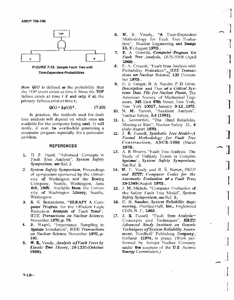
AMCP 706-196

TOP

5 _JL_

FIGURE 7-12. Sample Fault Tree with

Time-Dependent Probabilities

Now Q(t) is defined as the probability that the TOP event exists at time t. Since the TOP failure exists at time t if and cnly if all the primary failures exist at time t,

Q(t)=[q(t)V. (7-20)

In practice, the methods used for fault tree analysis will depend on which ones axe available for the computer being used. It will rarely, if ever, be worthwhile generating a computer program especially for a particular problem.

REFERENCES

1. D. F. Haasl, "Advanced Concepts in Fault Tree Analysis", System Safety Symposium, see Ref, 2.

2. System Safety Symposium, Proceedings of symposium sponsored by the Univer- sity of Washington and the Boeing Company, Seattle, Washington, June 8-9, 1965. Available from the Univer- sity cf Washington LUarary, Seattle, Washington.

3. S. N. Semanderes, "ELRAFT A Com- puter Program for the Efficient Togic Reduction Analysis cf Fault Trees", IEEE Transactions on Nuclear Science, November 1970,p. 79.

4. P. Nagel, "Importance Sampling in ^stan Simulation", IEEE Transactions on Nuclear Science, November 1970,p. 101.

5. W. E, Vesely, Analysis of Fault Trees by Kinetic Tree Theory, IN-1330 (October 1969).

6. W. E. Vesely, "A Time-Dependent Methodology for Fault Tree Evalua- tion", Nuclear Engineering and Dsskyi 13, 2 (August 1970) .

7. P. A. Crosetti, Computer Program for Fault Tree Analysis, DUN-5508 (April 1969).

8. P. A. Crosetti, "Fault Tree Analysis with Probability Evaluation"^JEEE Transac- tions on Nuclear Science, 132 (Novem- ber 1970) .

9. G. E. Greger, D. A. Snyder, P. D. Gross, Description and Uses of a Critical Sys- tems Data File for Nuclear Plants, The American Society of Mechanical Engi- neers, 345 East 47Ü1 Street, New York, New York 10017, January 9-12,1972.

10. M. M. Yarosh, "Accident Analysis", Nuclear Safety, 3,4 (1962).

11. L. Leonardini, "The Third Reliability Meeting at Riso", Nuclear Safety 11, 4 (July-August 1970) .

12. J. B. Fussell, Synthetic Tree Model—A Formal Methodology for Fault Tree Construction, ANCR-1098 (March 1973).

13. A. B. Mearns, "Fault Tree Analysis: The Study of Unlikely Events in Complex Systems' , System Safety Symposium, See Ref. 2.

14. W. E Vesely and R. E. Narum, PREP and KITT: Computer Codes for the Automatic Evaluation of a Fault Tree, IN-1349 (August 1970) .

15. J. M. Mchels, "Computer Evaluation cf the Safety Fault Tree Model", System Safety Symposium, see Ref. 2,

16. G. H. Sander, System Reliability Engi- neering, Prentice-Hall, Inc., Englewood Cliffs, N. J., 1963.

17. J. B. Fussell, "Fault Tree Analysis- Concepts and Techniques", NATO Advanced Study Institute on Generic Techniques of System Reliability Assess- ment, Nordhoff Publishing Company, Holland (1974, in press). (Work performed by Aerojet Nuclear Company under the auspices of the U S Atomic Energy Commission,)

~ 1

0

7-18-

AMCP 706-196

CHAPTER 8 FAILURE MODES AND EFFECTS ANALYSIS

8-0 LIST OF SYMBOLS

(CRh

(CR)S

ßu =

X,. =

CRiticality, viz, the portion of the system failure rate due to item f s failing in its mode ; system criticality, viz, failure rate failure mode frequency ratio of item / for the failure mode ;' loss probability of item i for failure mode j failure rate of item i

sum over all i car/

8-1 INTRODUCTION

Failure Modes and Effects Analysis (FMEA) (Ref. 1) is a technique for evaluating

the reliability of a design by considering potential failures and their effect on the system. It is a systematic procedure for determining the cause of failures and defining actions to minimize their effects. It can be applied at any level from complete systems to parts. The basic approach is to describe or identify each failure mode of an item, i.e., each possible way it can fail to perform its function. The analysis consists of identifying and tabulating the failure modes of an item, along with the effects of a failure in each mode. Following this analysis, corrective action can be taken to improve the design by determining ways to eliminate or reduce the probability of Occurrence of critical failure modes. This corrective action is performed by considering the relative seriousness of the effects of failures.

Criticality of an item is the degree to which satisfactory mission completion depends on the item. A mission usually has several tasks, e.g., a vehicle needs to provide prompt safe delivery of its cargo and safe delivery of its crew. A mission also is classified conveniently into several time phases. Some failure modes of an item will affect adversely some tasks and some phases of a mission, but not necessarily all of them. Some failure modes concerning crew and public safety are not failures in the ordinary sense;

for example, sharp edges which can cut a vehicle operator do not "fail", they are just there.

The principles of FMEA are straightforward and easy to grasp. The practice o- FMEA is tedious, time-consuming, and very profitable. It is best d«ne in conjunction with Cause-Consequence charts and Fault Tree analysis; both are explained in Chapter 7. The bookkeeping aspects, namely, the keeping track cf each item and its place in the hierarchy, are very important because mistakes are so easy t o make.

An FMEA also can be used as abasis for evaluating redesign, substitution, or replacements proposed during manufacture, assart bly, installaticn, and checkout phases.

The FMEA consists of two phases which provide a documented analysis for all critical components of a system. First, however, definitions of failure at the system, subsystem, and sometimes even part, level must be established.

Phase 1 is performed in parallel with the start of detail design and updated periodically throughout the development program as dic- tated by design changes. Phase 2 is performed before, or concurrently with, the release of detail drawings.

The Phase 1 lowing steps:

analysis consists of the fol-

(1) Constructing a symbolic logic block diagram, viz., the reliability diagram mentioned in Chapter 4 or a Cause- Consequenoe chart mentioned in Chapter 6.

(2) Performing a failure effect analysis, taking into account modes of failure' such as: (a) Open circuits (b) Short circuits (c) Dielectric breakdowns (d) Wear (e) Part-parameter shifts

(3) Proper system and item identification

(4) Preparation of a critical items list.

8-1

AMCP 706-196

During Riase 2, the results of Phase lare revised and updated as required by design changes. In addition, all items in the system are analyzed to determine their criticality with respect to the system.

8-2 PHASE 1

During this phase the following detailed steps are performed:

(1)A Symbolic Logic Block Diagram is constructed. This diagram is developed for the entire system to indicate the functional dependencies among the elements of the systsn and to define and identify its subsystems. It is not a functional schematic or a signal flow diagram, but a model for use in the early analysis to point out weaknesses. Figs. 8-1 and 8-2 show typical symbolic logic diagrams. Fig. 8-1 illustrates the functional dependency among the subsystems, sets, groups, and units that make up the system. Fig. 8-2 illustrates the functional dependencies among assemblies, subassemblies, and parts that make up one of the units in Fig. 8-1.

(2) A failure effect analysis is performed for each block in the symbolic logic block diagram, indicating the effect of item failure on the performance of the next higher level on the block diagram. Table 8-1 (Ref. 1) shows a typical group of failure modes for various electronic and mechancial parts, representing equipment cf the mid-1960's. The failure mode ratios are estimates and are to be revised on the basis of the user's experience. However, they can be used as a guide in performing a detailed failure effects analysis.

Fig. 8-3 illustrates a useful form for conducting a failure effect analysis. (Seealso Fig. 8-5 for an example of its use,) For each component in the system, appropriate information is entered in each column. Column descriptions are given in Table 8-2.

A numerical reference far all üBTE; in the symbolic logic block diagram must be provided by using a standard coding system, such as that specified in MIL-STD-16 (Ref. 2). All items below the set and group levels are identified using the scheme illustrated in Eg. 8-2. Items at and above the group and set levels are not subject to this standard nomenclature

scheme. These items can be assigned a simple code such as that illustrated in Fig. 8-1. in this illustration, the systaait is assigned a letter; and the subsystems, sets, and groups are assigned numbers in a specifically ordered sequence. As an example, the code S-23-01 designates the first group of the third set in the second subsystem of system S. The exact coding system used is not ,as important as making sure that each block in the diagram has its own number. Identical items (same drawing numbers) in different systems, or in the Same system but used in different applications, should not be assigned the same code number.

(3) During the failure effects analysis, a number of changes to the block diagrams may be required. Therefore, to minimize the number of changes in the coding system, it is recommended that the failure effects analysis be completed before assignment of code numbers is finalized.

(4) Based on the failure effects analysis, a list of critical items should be prepared. This fist will contain those items whose failure results in a possible loss, probable loss, or certain loss of the next higher level in the symbolic logic block diagram. All items that can cause system loss should be identified clearly in the list

8-3 PHASE2

This phase is implemented by performing the following steps:

(l)The symbolic logic block diagram, failure effects analysis, coding, and critical items list are reviewed and brought up-to- date.

(2) Criticality is assigned, based on the item applicable failure mode, the system loss probability, the failure mode frequency ratio, and the item unreliability. The analysis of criticality is essentially quantitative, based on a qualitative failure effects analysis,

Criticality CR, is defined by the equation :

(CR)U = aljPijX. (8-1)

where

8-2

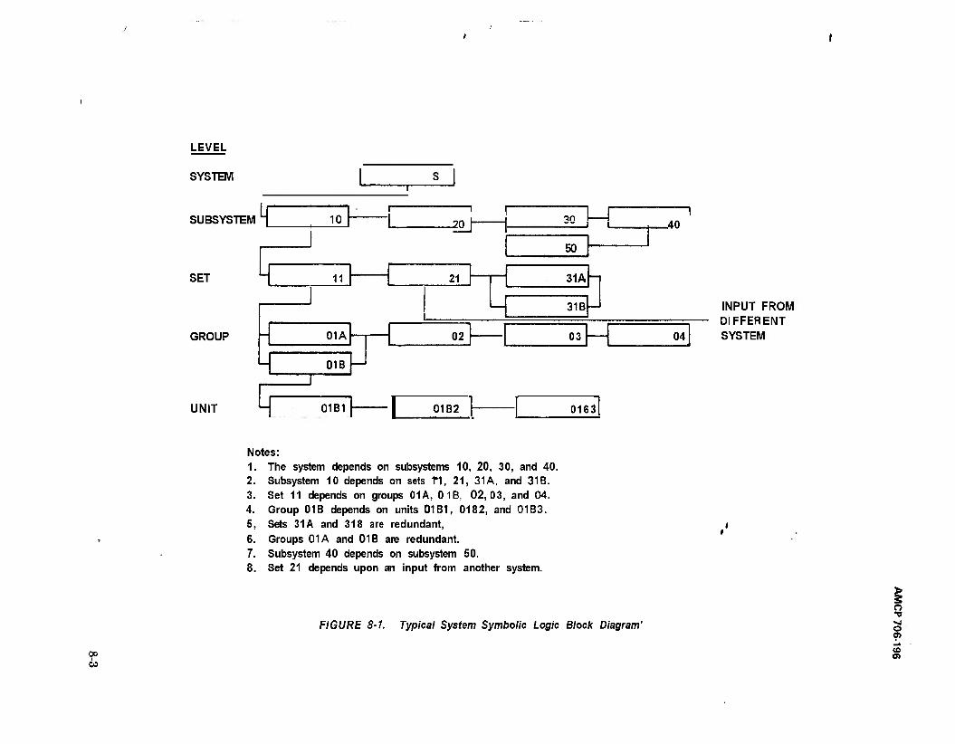
LEVEL

SYSTEM

SUBSYSTEM

SET

GROUP

UNIT

10 -\ r

-^y-

11 21

01A

01B —J

02

0 01B1 01B2

in J L

50

-40

31A-I

31B

03 04

INPUT FROM DIFFERENT SYSTEM

0163

Notes: 1. The system depends on subsystems 10, 20, 30, and 40. 2. Subsystem 10 depends on sets 1*1, 21, 31 A, and 31B. 3. Set 11 depends on groups 01A, 0 1B, 02,03, and 04. 4. Group 01B depends on units 01B1. 0182, and 01B3. 5. Sets 31A and 318 are redundant, 6. Groups 01A and 01B are redundant. 7. Subsystem 40 depends on subsystem 50. 8. Set 21 depends upon an input from another system.

FIGURE 8-1. Typical System Symbolic Logic Block Diagram'

00 I

CO

> 3 o

?

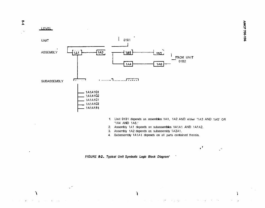
I LEVEL

UNIT

ASSEMBLY q 1A1

SUBASSEMBLY rr

1A2

1A1A1Q1 1A1A1Q2 1A1A1C1 1A1A1C2 1ATA1R1

01B1

_J

Am}-

1A4

J25_

1A6

> o

O 0> <U CO

FROM UNIT 01B2

1. Unit 01B1 depends on assemblies 1A1, 1A2 AND either '1A3 AND 1A5' OR '1A4 AND 1A6.'

2. Assembly 1A1 depends on subassemblies 1A1A1 AND 1A1A2, 3. Assembly 1A2 depends on subassembly 1A2A1, 4. Subassembly 1A1A1 depends on all parts contained therein.

FIGURE 8-2. Typical Unit Symbolic Logic Block Diagram'

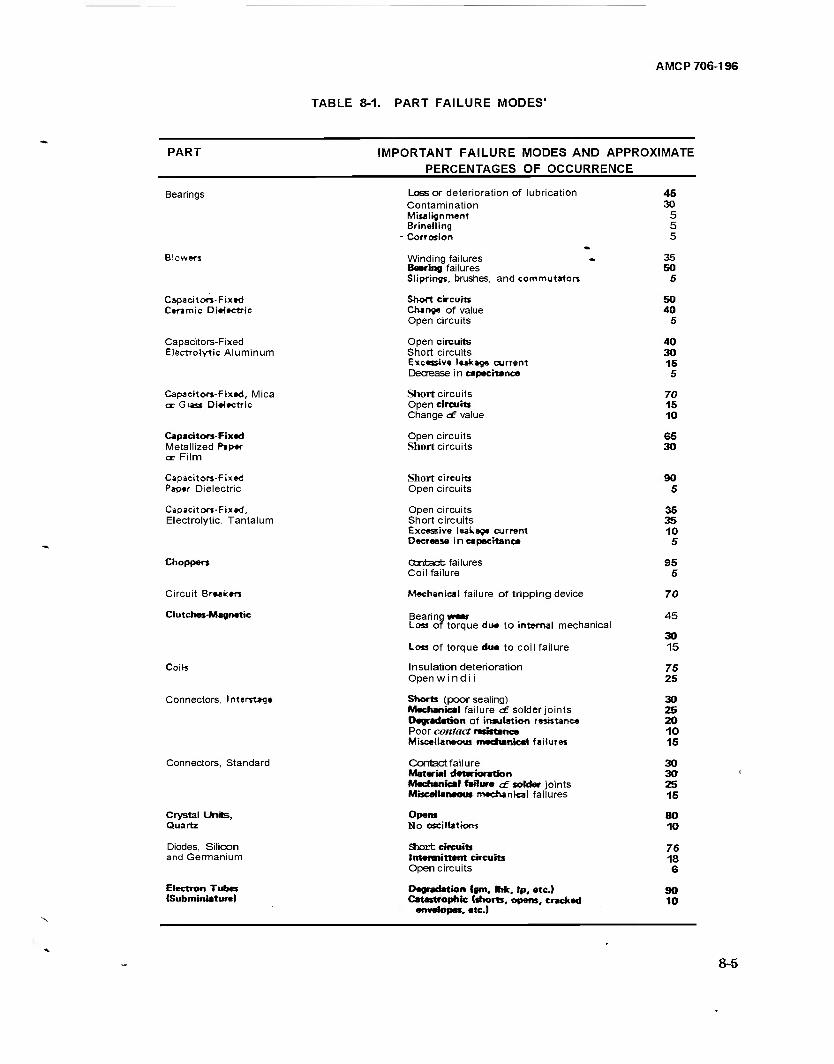
AMCP 706-196

TABLE 8-1. PART FAILURE MODES'

PART IMPORTANT FAILURE MODES AND APPROXIMATE PERCENTAGES OF OCCURRENCE

Bearings

Blowers

Capacitors-Fixed Ceramic Dielectric

Capacitors-Fixed Electrolytic Aluminum

Capacitors-Fixed, Mica cr Glass Dielectric

Capacitors-Fixed Metallized P*p*r cr Film

Capacitors-Fixed Paper Dielectric

Capacitors-Fixed, Electrolytic. Tantalum

Choppers

Circuit Breakers

Clutches-Magnetic

Coils

Connectors, Interstage

Connectors, Standard

Crystal Units, Quartz

Diodes, Silicon and Germanium

Electron Tubes (Subminiature)

Loss or deterioration of lubrication Contamination Misalignment Brinelling Corrosion

Winding failures Bearing failures Sliprinss, brushes, and commutators

Short circuits Change of value Open circuits

Open circuits Short circuits Excessive leakage current Decrease in capacitance

Short circuits Open circuits Change <£ value

Open circuits Short circuits

Short circuits Open circuits

Open circuits Short circuits Excessive leakao» current Decrease i n capacitance

Cfcnbact failures Coil failure

Mechanical failure of tripping device

Bearing Loss of torque due to internal mechanical

Loss of torque doe to coil failure

Insulation deterioration Open wind i i

Shorts (poor sealing) Mechanical failure <f solder joints Degradation of insulation resistance Poor contact resistance Miscellaneous mechanical failures

Contact failure Material deterioration Mechanical failure <± solder joints Miscellaneous mechanical failures

Opens No oscillations

Short circuits Intermittent circuits Open circuits

Degradation (om, Hik, Ip, etc.) Catastrophic (shorts, opens, cracked

envelopes, etc.)

45 30 5 5 5

35 50 5

50 40 5

40 30 15 5

70 15 10

65 30

90 5

35 35 10 5

95 5

70

45

30 15

75 25

30 25 20 10 15

30 30 25 15

80 10

76 18 6

90 10

8-5

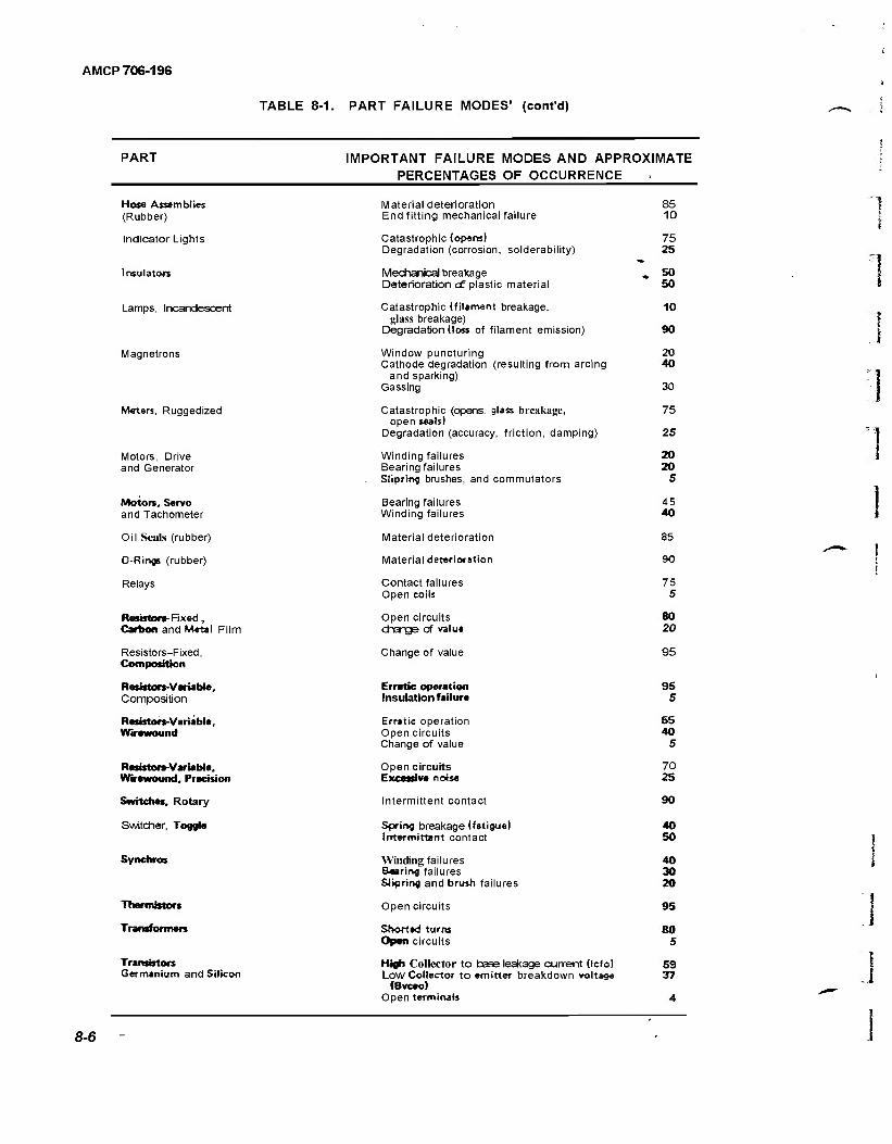
AMCP 706-196

TABLE 8-1. PART FAILURE MODES' (cont'd)

PART IMPORTANT FAILURE MODES AND APPROXIMATE PERCENTAGES OF OCCURRENCE

Hose Asamblies (Rubber)

Indicator Lights

Insulators

Lamps, Incandescent

Magnetrons

Meters, Ruggedized

Motors, Drive and Generator

Motors, Servo and Tachometer

Oil Seals (rubber)

O-Rings (rubber)

Relays

Resistors- Fixed, Carbon and Metal Film

Resistors-Fixed, Composition

Resistors-Variable, Composition

Resistors-Variable, Wirewound

Resistors-Variable. Wirewound, Precision

Switches, Rotary

Switcher, Toggle

Synchros

Thermistors

Transformers

Transistors Germanium and Silicon

Material deterioration End fitting mechanical failure

85 10

Catastrophic (opens) Degradation (corrosion, solderability)

75 25

Mechanical breakage Deterioration <£ plastic material

. 50 50

Catastrophic (filament breakage, glass breakage)

Degradation {loss of filament emission)

10

90

Window puncturing Cathode degradation (resulting from arcing

and sparking) Gassing

20 40

30

Catastrophic (opens, glass breakage, open teals)

Degradation (accuracy, friction, damping)

75

25

Winding failures Bearing failures Sliprmg brushes, and commutators

20 20

5

Bearing failures Winding failures

45 40

Material deterioration 85

Material deterioration 90

Contact failures Open coils

75 5

Open circuits change of value

SO 20

Change of value

Erratic operation Insulation failure

Erratic operation Open circuits Change of value

Open circuits Excessive noise

Intermittent contact

Spring breakage (fatigue) Intermittent contact

Winding failures Bearing failures Slipring and brush failures

Open circuits

Shorted turns Open circuits

High Collector to base leakage current (Icfo) Low Collector to emitter breakdown vortege

(Bvceol Open terminals

95

95 5

55 40

5

70 25

90

40 50

40 30 20

95

80 5

59 37

8-6

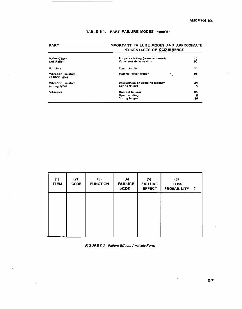
AMCP 706-196

TABLE 8-1. PART FAILURE MODES" (cont'd)

PART IMPORTANT FAILURE-MODES AND APPROXIMATE PERCENTAGES OF OCCURRENCE

Valves-Check and Relief

Poppets sticking (open or closed) Valve seat deterioration

40 50

Varistors

Vibration Isolators (rubber type)

Vibration Isolators (spring type)

Vibrato«

Open circuits

Material deterioration

Degradation of damping medium Spring fatigue

Contact failures Open winding Spring fatigue

95

85

80 5

80 5

15

(1) ITEM

(2J CODE

(3) FUNCTION

(4) FAILURE MODE

(5) FAILURE EFFECT

(6) LOSS

PROBABILITY, ß

FIGURE 8-3. Failure Effects Analysis Form'

8-7

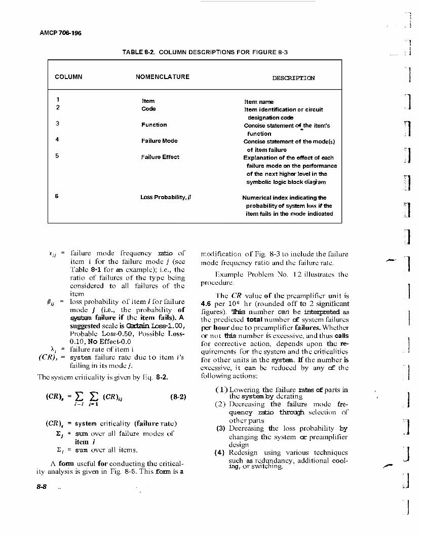
AMCP 706-196

TABLE 8-2. COLUMN DESCRIPTIONS FOR FIGURE 8-3

COLUMN NOMENCLATURE DESCRIPTION

1 Item Item name 2 Code Item identification or circuit

designation code 3 Function Concise statement of the item's

function 4 Failure Mode Concise statement of the mode(s)

of item failure 5 Failure Effect Explanation of the effect of each

failure mode on the performance of the next higher level in the symbolic logic block diagram

6 Loss Probability, ß Numerical index indicating the probability of system loss if the item fails in the mode indicated

Pij =

(CR),

failure mode frequency ratio of item i for the failure mode ;' (see Table 8-1 for an example); i.e., the ratio of failures of the type being considered to all failures of the item loss probability of item / for failure mode j (i.e., the probability of system failure if the item fails). A suggested scale is Gatlcun Loss-1.00, Probable Loss-0.50, Possible Loss- 0.10,NoEffect-0.0 failure rate of item i system failure rate due to item i's failing in its mode ;'.

The system criticality is given by Eq. 8-2.

(CR). = ZI (CR)U (8-2) i = l /«l

(CR), = system criticality (failure rate)

TZj - sum over all failure modes of item /

£, = sum over all items.

A form useful for conducting the criticality analysis is given in Fig. 8-5. This form is a

modification of Fig. 8-3 to include the failure mode frequency ratio and the failure rate.


The CR value of the preamplifier unit is 4.6 per 106 hr (rounded off to 2 significant figures). This number can be interpreted as the predicted total number of system failures per hour due to preamplifier failures. Whether or not this number is excessive, and thus calls for corrective action, depends upon the requirements for the system and the criticalities for other units in the system. If the number is excessive, it can be reduced by any of the following actions:

(1) Towering the failure rates of parts in the system by derating

(2) Decreasing the failure mode frequency ratio through selection of other parts

(3) Decreasing the loss probability by changing the system or preamplifier design

(4) Redesign using various techniques such as redundancy, additional cooling, or switching.

J

8-8

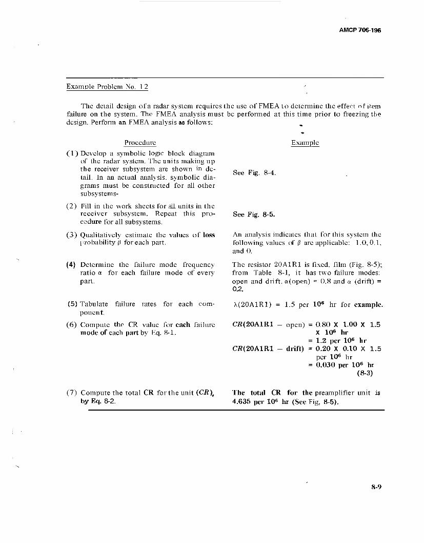
AMCP 706-196


The detail design of a radar system requires the use of FMEAto determine the effect of item failure on the system. The FMEA analysis must be performed at this time prior to freezing the design. Perform an FMEA analysis as follows:

Procedure

(1) Develop a symbolic logic block diagram of the radar system. The units making up the receiver subsystem are shown in detail. In an actual analysis, symbolic diagrams must be constructed for all other subsystems-

(2) Fill in the work sheets for all units in the receiver subsystem. Repeat this procedure for all subsystems.

(3) Qualitatively estimate the values of loss probability ß for each part.

(4) Determine the failure mode frequency ratio a for each failure mode of every part.

Example

See Fig. 8-4.

See Fig. 8-5.

An analysis indicates that for this system the following values off? are applicable: 1.0,0.1, and 0.

The resistor 20A1R1 is fixed, film (Fig. 8-5); from Table 8-1, it has two failure modes: open and drift, a(open) = 0.8 and a (drift) = 0.2.

(5) Tabulate failure rates for each component.

(6) Compute the CR value for each failure mode of each part by Eq. 8-1.

\(20A1R1) = 1.5 per 10« hr for example.

CÄ(20A1R1

CR(20A1R1 -

open) = 0.80 X 1.00 X 1.5 X 106 hr

= 1.2 per 106 hr drift) = 0.20 X 0.10 X 1.5

per 106 hr = 0.030 per 10s hr

(8-3)

(7) Compute the total CR for the unit (CR)e

by Eq. 8-2. The total CR for the preamplifier unit is 4.635 per 106 hr (See Fig, 8-5).

8-9

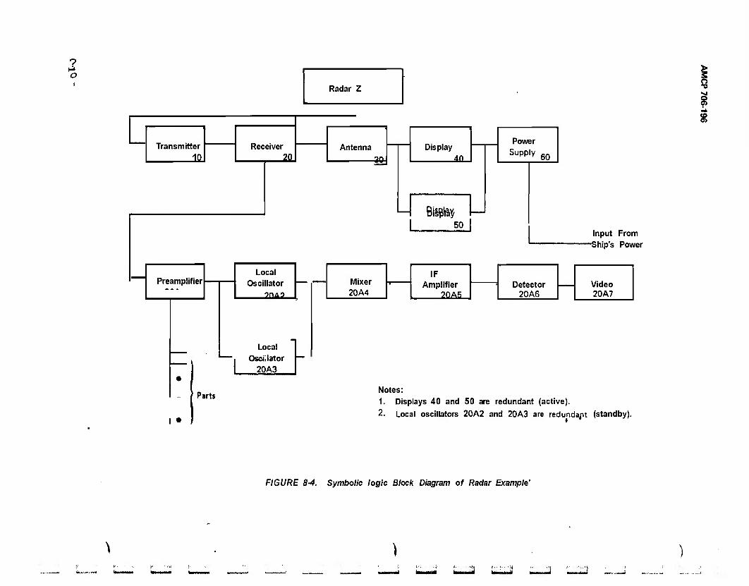
O

Radar Z a

Transmitter

10

Preamplifier

Receiver

-2! Antenna

Local

Oscillator

20A2-

Local

Oscillator

20A3

Parts

I •

-30-

Display

_4Q_

u Bisptey 50

Mixer 20A4

IF Amplifier 20A5

Power Supply 60

Detector 20A6

Input From -Ship's Power

Video 20A7

Notes: 1. Displays 40 and 50 are redundant (active).

2. Local oscillators 20A2 and 20A3 are redundaju (standby).

$

FIGURE 8-4. Symbolic logic Block Diagram of Radar Example'

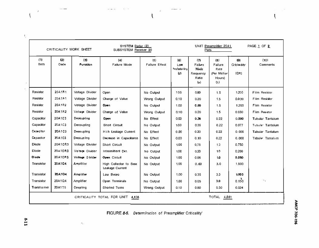
CRITICALITY WORK SHEET SYSTEM Radar (2)

SUBSYSTEM Receiver 20 UNIT Preamplifier 20A1 PAGE 1 OF 2

Parts

(1) (2) (3) (41 (5) (6) (7) (8) (9) (10) Item Code Function Failure Mode Failure Effect Loss

'robability

(0)

Failure

Mode

Frequency

Ratio

M

Failure

Rate

(Per Mtllior

Hours)

M

Cr itica lity

(CR)

Comments

Resistor 20A1R1 Voltage Divider Open No Output too 0.80 1.5 1.200 Film Resistor

Resistor 20A1R1 Voltage Divider Change of Value Wrong Output 0.10 0.20 1.5 0.030 Film Resistor

Resistor 20A1R2 Voltage Divider Open No Output 1.00 0.80 1.5 1.200 Film Resistor

Resistor 20A1R2 Voltage Divider Change of Value Wrong Output 0.10 0.20 1.5 0.030 Film Resistor

Capacitor 20A1C3 Decoupling Open No Effect O.OD 0.36 0.22 0.000 Tubular Tantalum

Capacitor 20A1C3 Decoupling Short Circuit No Output 1.00 0.35 0.22 0.077 Tubular Tantalum

Capeeitor 20A1C3 Decoupling H i h Leakage Current No Effect 0.00 0.20 0.22 0.000 Tabular Tantalum

Capacitor 20A1C3 Decoupling Decrease in Capacitance No Effect 0.00 0.10 0.22 0.000 Tabular Tantalum

Diode 20A1CR3 Voltage Divider Short Circuit No Output 1.00 0.75 1.0 0.750

Diode 20A1CR3 Voltage Divider Intermittent Ckt, No Output too 0.20 1.0 0.200

Diode 20A1CR3 Vortag« Divider Open Circuit No Output 1.00 0.06 1.0 0.050

Transistor 20A1Q4 Amplifier High Collector to Base

Leakage Current No Output 1.00 0.60 3.0 1.800

Transistor 20A1Q4 Amplifier Low Bvceo No Output 1.00 0.35 3,0 1.050

Transistor 20A1Q4 Amplifier Open Terminals No Output 1.00 0.05 3D 0.150

Transformer 20A1T5 Coupling Shorted Turns Wrong Output 0.10 0.80 0.30 0.024

CRITICALITY T OTAL FOR UNIT 4,835 TOTAL 4361

FIGURE 8-5. Determination of Preamplifier Criticality'

> o

o

CO CD

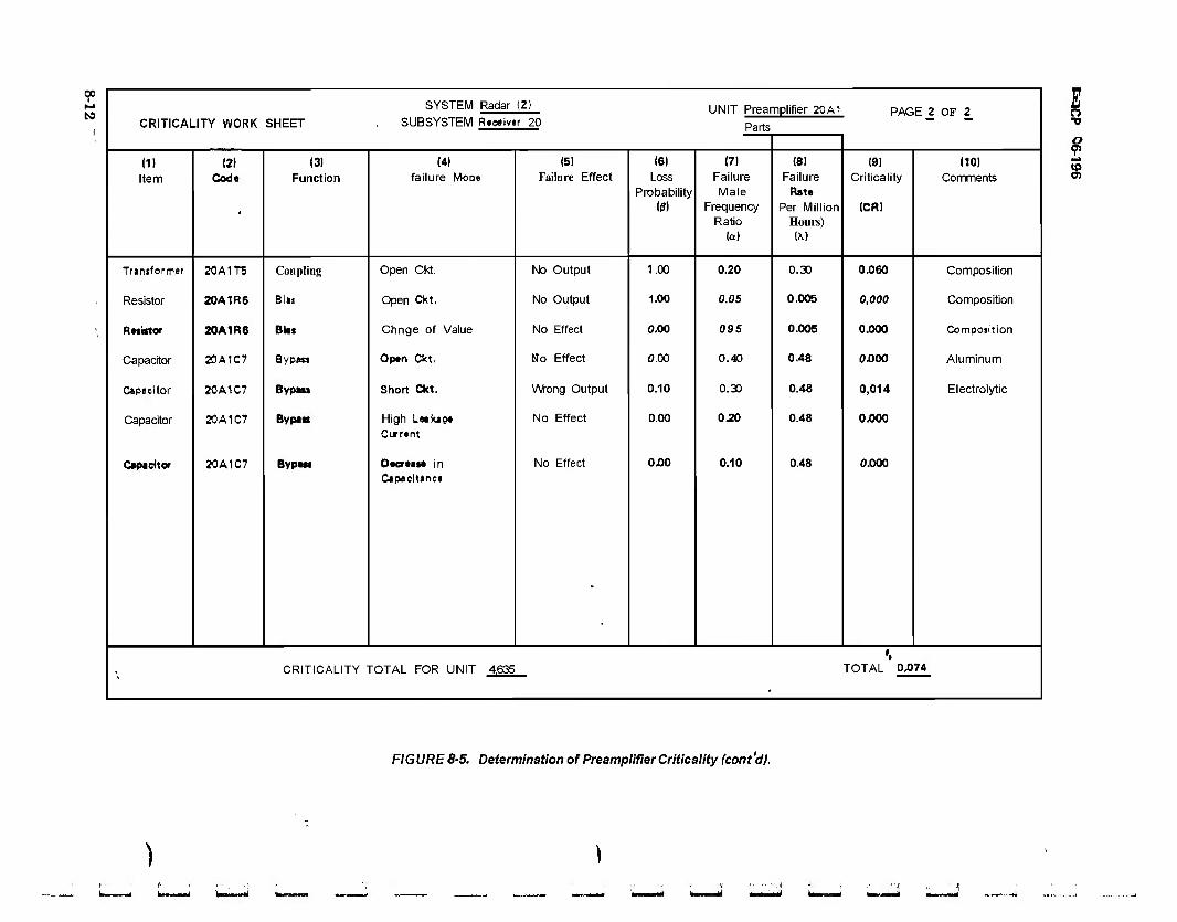
00 I

to SYSTEM Radar (2) UNIT Preamplifier 20A1 PAGE 2 OF 2

CRITICALITY WORK SHEET SUBSYSTEM Raealvar 20 Parts

ID (2) (3) (4) (5) (6) (7) (8) (9) (10) Item Cod« Function failure Mode Failure Effect Loss

Probability If?)

Failure Male

Frequency Ratio

Failure Rate

Per Million Hours) M

Criticality

(CR)

Comments

Transformer 20A1TS Coupling Open Ckt. No Output 1.00 0.20 0.3O 0.060 Composition

Resistor 20A1R6 Bits Open Cfct, No Output 1.00 0.05 0.005 0,000 Composition

R Mi*tor 20A1R6 Bias Chnge of Value No Effect 0.00 095 0.005 0.000 Composition

Capacitor 20A1C7 Bypass Opan Ckt, No Effect 0.00 0.40 0.48 0.000 Aluminum

Capacitor 20A1C7 Bypatt Short Ckt. \AAxsng Output 0.10 0.30 0.48 0,014 Electrolytic

Capacitor 20A1C7 By pas High Laakao» Current

No Effect 0.00 0.20 0.48 0.000

Capacitor 20A1C7 BypaM Oacraasa in Cipaeltane»

No Effect 0.00 0.10 0.48 0/100

'- CRITICALITY " FOTAL FOR UNIT 4,635 TOTAL 0,074

I o ■p

o Ml

8

FIGURE 8-5. Determination of Preamplifier Criticality (cont'd).

AMCP 706-196

8-4 COMPUTER ANALYSIS

A computer can be quite useful in performing an FMEA, since a large number of computations and a large amount of record keeping are often required for systems of reasonable size.

In the failure effects portion of the analysis the computer is used primarily for function evaluation, using performance models. On the assumption that the computer program contains the design equations relating system outputs to various design parameters, each item is allowed to fail in each one of its modes, and the effect on the system is computed.

Several computer programs are available for evaluating circuits. The NET-1 (Ref. 3) network analysis program can be used for a failure effects analysis of a circuit containing transistors and passive circuit elements. The value of all of the circuit performance parameters would be printed out for each abnormal condition. NET-1 does not automatically consider failure modes of circuit parts such as shorts and opens; investigation of these require manually setting up a new run for each set of values of the parts. A shorted resistor would have zero resistance and an open resist- or would have infinite resistance.

Circuit analysis programs such as ECAP (Electronic Circuit Analysis Program) (Ref. 4), which accept a topological input description of the circuit and synthesize the circuit equations, can be used to evaluate failure effects, but computer running time can become excessive since the circuit equations may have to be generated over again for each run. For extreme failure modes such as an open or a short of a part, the circuit configuration is changed and a completely new solution is required.

The AMAP (Automated Failure Mode Analysis Program)-(Ref 5) is a circuit analysis program that automates the failure effect analysis for DC circuits. It repeatedly solves the circuit equations, computing and printing

circuit node voltages, for failure modes such as open and short of parts and shorts between all node pairs. However, AMAP includes only resistors, diodes, transistors, power supplies, and nodes. This automated approach to failure effects analysis can be used effectively in other types of systems such as structures and propulsion systems, but no programs are known which providelhese capabilities.

Two other programs that can be used for FMEA are:

(1)IM 045-NAA: Analyzes failure mode effects at system, subsystem, or part level. (Ref. 6)

(2) IM 066-NAA: Revision of IM 045-NAA. (Ref. 8)

(3) IM 063-NAA: Analyzes failure mode effects at system, subsystem, or part level. (Ref- 7).

REFERENCES

1. Bureau of Ships Reliability Design Hand- book, NAVSHIPS 94501, Change 2, Fleet Electron its Effectiveness Branch, Bureau of Ships, 28 February 1965.

2. MIL-STD-16, Electrical and Electronic Reference Designations.

3. A. F. Malmberg, "NET-1 Network Analysis Program". Proceedings of the Eleventh National Symposium on Reli- ability and Quality Control, 510-517, 1965.

4. H. N. Tyson, Jr., et al., "The IBM Elec- tronic Circuit Analysis Program (ECAP)". Proceedings of the 1966 An- nual Symposium on Reliability, 45-65 (1966).

5. D. A. Hausrath and R. Ranalli, "Com- puter Studies of Abnormally Operating Circuits", Proceedings of the 1966 An-, nual Symposium on Reliability, 66-86 (1966).

6. K. R. Brown, Failure Mode Analysis Pro- gram (IM-04 5)> Report No. 63-C5G-043-20-36, North American Aviation, Inc., Downey, California, September 1963.

8-13

AMCP 706-196

7. K. L. Bond and D. S. Kordell, Ground 8. D. S. Kordell, Airborne Failure Mode Support Equipment Mode Analysis Analysis Program (IM-066), Report No. Program (IM-063), Report No. 64-CT-043-14-14, North American Avia- 64-CT-043-14-41, North American Avia- tion, Inc., Downey, California, January tion, Inc., Downey, California, ^ferch 1964, AD-459 212. 1964. 1

1 1

1 1 1

1 1

8-14

AMCP 706-196

CHAPTER 9 MODELS FOR FAILURE

9-0 LEST OF SYMBOLS

A = a,b = Cdf =

CtA =

D = d = E =

e = F = f =

°* = G, = 8$ —

gauf =

gaufc =

Gtf = h = / =

MS = n = n =

NT, Ns = P =

Pdf = Po -

PfLfä = PSM =

Q = Sf =

T = t,u =

u =

y a

ß

7

parameter in Eq. 9-50 width and length of a plate Cumulative distribution function coefficients in linear expansion, defined by Eqs. 9-31C, D diameter design load factor Young's modulus, modulus of elasticity (units of stress) strain (dimensionless) strength stress Cdf {4} Sf{4>} pdf{<t>} Cdf for a standard s-normal (Gaussian) variable Sf for a standard s-normal (Gaussian) variable parameters in Eq. 9-50 thickness of a plate length margin of safety limit load factor number of xt's parameters in Eq. 9-50 power, Eq. 9-50 probability density function parameter in Eq. 9-50 load, limit load, design load probabilistic safety margin probability of failure Survivor function, Sf = 1 — Cdf temperature, Eq. 9-50 subscripts -*■ tensile, ultimate stress or strength, random variable randcm variable i a function scale parameter (same units as «) shape parameter (dimensionless) location parameter (same units as u)

7*

8

nR,nE

& = 0

coefficient of variation, defined by Eq. 9-3 IB elongation defined by Eq. 9-36 failure rates, see Eqs. 9-49, 9-50 mean value of 4> application factors for resistor failure rates failure rate term, see Eq. 9-49 standard deviation <f> parameter s of a distribution parameter k of a distribution general name for a random variable, it can be f, F, orF - f

9-1 INTRODUCTION

Two main classifications of material behavior are introduced for "things that cause failure", i.e.,

(1) Stress-strength. Any stress below the failure-stress (strength) produces only a reversible effect (such as elongation or increased electric-current flow), When the stress is removed, there is no damage—no evidence that the stress was ever there. A good example is tensile stress in a steel bar.

(2) Damage-endurance. The application of a damager (such as a corrosive fluid) produces damage that cumulates (usually irrevers- ibly). When the damager is removed, the damage remains; if the damager is applied again, the damage increases again. The item fails when the damage exceeds the endurance of the material. A good example is fatigue damage in aluminum alloys due to fluctuating bending stresses.

Both can be treated either deterministically or, probabilistically. Data on probabilistic behavior are very difficult (expensive and time consuming) to obtain.

The simple explanations of stress-strength and damage-endurance belie the complicated nature of failure in materials. Structural materials have many modes of failure; e.g., tensile, bending, shear, corrosion, impact, ductile, brittle, fatigue, corrosion-fatigue, stress-cor-

9-1

AMCP 706-196

rosion, embrittlement, fretting corrosion, and mechanical abrasion. A description of a steel alloy as "high strength" can be very misleading. Usually, in that case, only uniaxial tension failure is implied, and all other failure modes are neglected. The impact strength, car ductile-brittle transition temperature might be very poor.

Generally speaking, when specialty materials are being used, a specialist on each material ought to be consulted. Metallurgists and material engineers are the most likely consult- ants in this area. MIL-HDBK-5 (Ref. 3) is a good source of material, but does not cover all failure modes. Handbooks such as Refs. 10, 11 are helpful. Ref. 12 is a good book which describes some failure modes of metals and gives case histones. Every designer should read some case histories of structural failures. It can be a sobering, humble experience.

This chapter introduces several types of mathematical analysis; it does not discuss the detailed knowledge of materials that is so necessary to good structural design. The designer ought also to be aware that it is one thing to specify a material with certain guaranteed properties; it is another thing to get the prop erties, month after month, on every bit of material delivered under that specification.

The stress/strength notation used in this chap ter is taken from MIL-HDBK-5 (Ref. 3, July 72 update). It uses F for strength and f for Stress.

9-2 «DETERMINISTIC STRESS-STRENGTH

A general stress-strength model can be stated.

"There exist a scalar S and a value of that scalar S* such that the part fails if and only if S > S* (S* is the strength), values of S < S* do no damage to the part; in fact, damage less than failure, has no meaning. S can only depend reversibly on the environment (mechanical, electric, fluid, temperature, etc.) of the part."

The breakdown voltages cf semi conductor devices and tensile failures of structural materials are presumed to be adequately described by this model.

Even in mechanics where this model is applicable, determining the parameter S is not always easy. Ref. 13 lists six stress-strength models for failure with multiaxial stresses: maximum principal stress (Rankine), maximum shear stress (Coulomb), maximum strain energy (Beltrami), maximum distortion energy (Huber, von Mises, Hencky), maximum strain (Saint-Venant), and internal energy (Mohr). For ductile materials the distortion energy model is best when the tension/compression properties are the same, and the internal energy model is best when they are not the same (Ref. 13).Safety codes tend to use the maximum shear model for ductile materials and maximum principal stress model for brittle ones. In each case, the-strength is derived by comparison with the parameter of the model when evaluated for uniaxial stress. This detailed example illustrates the complexity of the subject even in a situation that "everyone knows and understands" and where generalization is easy. In this example, even though more than one dimension of stress are combined, they are of the same nature, viz., mechanical stress. The complexity that can arise when this is not true is not often appreciated.

The criteria for failure have been implicitly presumed to exist. Failure must be explicitly defined, and S* depends on that definition. For example, there are both yield and ultimate strengths of metals which are defined differently, and, for semiconductor devices, the breakdown voltages usually are defined in terms of a specific current cor a change in current.

It is conceptually easy to extend the simple stress-strength theory to the case where several different failure modes exist. If they are independent, the resultant strength is fairly simple, if rot, the synergistic effects can be taken into account in principle. In practice, the problem is difficult if not impossible and is not pursued very far. Instead, simplifying assumptions are made and life marches on.

9-2.1 TENSILE STRENGTH

This paragraph deals with tensile/com- pressive stress. The same principles are appli-

9-2

AMCP706 196

cable to other mechanical stress and to more generalized "stresses" such as electric field. MIL-HDBK-5 (Ref. 3) ought to he consulted for a more comprehensive discussion. No mechanical designer ought ever to be without the latest version of MIL-HDBK-5.

A structural nonviscoelastic material undergoes strain when a uniaxial stress is applied. Most such materials have a linear region, i.e., Hooke's law holds as long as the stress is not too high.

/, = eE (9-1)

where ft = tensile stress, force/area e = strain (elongation/original length),

dimensionless. Strain is often given "units" of inches/inch.

E = modulus of elasticity, force/area.

Even though the modulus of elasticity is independent of stress and strain in the linear region (by definition of linear region), it does depend on temperature and on material composition and structure. Although for ferrous alloys, it is remarkably independent of composition and structure.

Beyond the limits of Hooke's law, strain increases as the stress increases, but the linearity ceases. Plotting stress against strain for any material gives the tensile-test diagram, Fig. 9-1. Fig. 9-l(A) is typical of a ferrous material such as carbon or alloy steel, and Fig. 9-l(B) is typical of some nonferrous materials such as brass and aluminum and of some stainless steels. The important distinction between the two curves is that Fig. 9-l(A) shows a definite inflection point and change of curvature, whereas Fig. 9-l(B) does not.

Certain points on these curves have been defied and are important material properties. Consider first the stress-strain curve in Fig. 9-1 (A). The region from zero to A is a reasonably straight line, showing that the material is obeying Hooke's law (say, within 0.1%orso). This leads to the definition of point A as the proportional limit. It readily can be seen that the equation of this line is the familiar f, = eE, where E is the slope.

Beyond point A linearity ceases, and at point B a sudden increase in elongation takes place with little or no increase in load, This

phenomenon is called yielding, and point B is called the yield point of the material. The stress associated with this point is the yield stress. Once this point is reached in the material, all load can be removed from the specimen and the stress returned to zero, but a residual strain, permanent set, will remain. Any permanent set is usually considered detrimental to a structural member.

Beyond point B, stress and elongation continue to change until the maximum stress, the ultimate stress, is reached at point C. Rup- ture of the material occurs at point D, which is reached without any increase in stress or load. In fact, decreasing the load beyond point C will not necessarily avert fracture, The curve of Fig. 9-l(A) exhibits this definite, observed yield point; one which easily can be recognized as it occurs during a tensile test. The region nearAf is very machine dependent. The fall-off in stress is caused by the slow-rate of pulling the specimen by the tensile machine.

The materials represented by Fig. 9-l(B), however, do not exhibit as definite a yield point, although the other points on the curve are defined in the same manner as their coun- terparts in Fig. 9-1 (A). In materials such as those represented by Fig. 9-1 (B), it generally is accepted that the yield point is the stress at the 0.2 percent "offset point", viz., the point at which the actual strain exceeds the linearly extrapolated strain by 0.002. To find this point, draw a line through the point (e = 0.002, S = 0) with a slope of E; where this line intersects the curve is the 0.2 percent yield point of the material.

Similar diagrams will result for tests in compression and in shear, although the modulus might be different. These structural prop erties are listed in tables in various handbooks, such as MIL-HDBK-5 (Ref. 3) whitfh has joint military service approval.

The properties presented in most handbooks are room-temperature properties. If a problem involves elevated temperatures, the allowable properties must be those for the elevated temperature; these are usually lower than the room temperature properties. Although the tables in MIL-HDBK-5 generally are room-temperature values, some curves do give the effects of temperature. If these curves

9-3

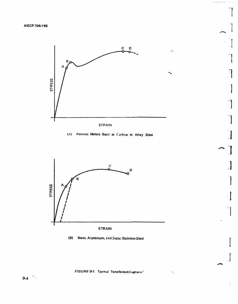
AMCP 706-196

STRAIN

(A) Ferrous Metals Such as Carbon or Alloy Steei

STRAIN

(B) Brass, Aluminum, and Some Stainless Steel

9-4

FIGURE 9-1. Typical Tensiletest Diagrams'

AMCP 706-196

are inadequate, the Military Specifications governing the specific materials ought to pro- sent the elevated-temperature data required if they exist. It is easy for the designer to be lulled by a false sense of security by data in handbooks and supplier's literature. Not much really is guaranteed unless:

(l)The data to be guaranteed appear in the purchase order

(2) The receiving inspection actually checks it

(3) No waivers are given for discrepant material.

9-2.2 SAFETY FACTORS, LOAD FAC- TORS, AND MARGIN OF SAFETY

Load analysis is used to determine the loads which exist on the structure under consideration. Stress analysis is the means by which the designer determines whether his structure is adequate to withstand these loads without failure. Since no universal criteria for failure exist, they must be. defined to suit each problem. Mechanical failure can be divided into four general categories:

(1) Rupture. A physical parting of the fibers or grains of the material when the ultimate (tensile or shear) stress is exceeded.

(2) Yielding. The stress in the material exceeds its yield stress in tension, compression, or shear and permanent settakes place,

(3) Buckling. The stress exceeds an allowable stress that is determined by the geometry of the loaded member. Fear example, columns buckle at a stress which depends upon the length to radius-of-gyration ratio; thin flat panels buckle under a shear stress that depends upon the ratio of panel width to metal thickness.

(4) Deflection. Since all structural members deflect under load, this deflection becomes a failure criterion in certain problems, particularly those associated with vibration environments.

Some confusion exists among designers in the definition and use of safety factors, load factors, and margins of safety.

Therefore, to clarify their use in the fol- towing discussion, they are defined here.

Safety Factors. Safety factors are numbers representing a degree of uncertainty in the expected load, the material properties, or other pertinent data of the problem. These are applied to reduce the nominal properties of the material to a lower value that, shall then not be exceeded in „the design calculations. For example, tensile ultimate stress for 20241'4 aluminum alloy extruded bar stock is published in MIL-HDBK-5 (July 72 update) as 57,000 psi (for < 0.50 in. diameter; L,A basis). A safety factor of 3 applied to a member designed in the alloy would reduce this ultimate stress to an allowable stress of 19,000 psi. Fatigue from repeated or cyclic loads sometimes is treated by applying a safety factor to the ultimate stress of the material but it is better to use fatigue curves if they are available.

Abrupt changes in cross section, notches, grooves, or other discontinuities ought to be avoided in the design of structural parts, since these function as stress raisers. When these cannot be avoided, the designer must apply specific design factors in these local areas. Many handbooks publish tables and examples or guides to the magnitude of design factors which can be used and which are considered adequate. However, the engineer must be cau- tioned to use care in his selection of a design factor from a handbook since the degree of uncertainty of the data usually is not presented,

Load Factors, Load factors are numbers representing multiplying factors applied to the load on the structure. Loads can be caused by any number of environmental conditions such as an aircraft in arrested landing or in catapult take-off, a truck proceeding across country on rough or bumpy roads, or a ship subjected to an underwater blast or the firing of its own guns. Load factors usually ane expressed in terms oig, or gravity units- Since the load analysis has been performed under a 1-g condition, the load factors easily can be taken into account by multiplying calculated loads and reactions by the proper load factor. By this simple means, it is easy to take into account different loading conditions in different directions or,at different points in

9-5

AMCP 706-196

the structure without directly affecting the original load analysis.

LwaLt Lowd. Limit load is the load that the structure is expected to experience—it is the limit of the load on the structure.

Design Load. Design load is larger than the limit load and is used to compare the stress in the structural members. Usual practice for airborne equipment is to define:

Design Load = 1.5 X (limit load) (9-2)

Although the 1.5 design load factor can be modified by the individual designer, it is recommended that the range of selection remain between 1.5 and 2.0. Larger factors tend to be too conservative and result in an over- weight and more costly structure.

Margin of Safety. Margin of safety MS is the fraction increase of the computed stress required to equal the allowable stress. It is calculated by the relationship:

MS =

(allowable) s stress /

(compi uted] ess /

computed stress (9-3)

If the computed stress equals the dowable stress, there is obviously a zero margin of safety, and failure is imminent. Lherefore, a positive margin is desired in all design, and experience has shown that a 15-percent margin is adequate for most purposes. Exceptions should be made to this rule in some instances where a single bolt carries the load in tension (50-percent nargin recommended), or where a particularly severe design condition has a negligible possibility of occurrence (zero margin may be acceptable).

Allowable Stress. An allowable stress is defined as the stress that a member may be allowed to reach (zero margin) and beyond which failure as previously defined is imminent. When yielding is the failure criterion, the allowable stress is the yield stress as modified by any imposed safety factors. For all other cases (e.g., when rupture is the failure criterion), the allowable stress is the ultimate stress of the material (whether taken from a handbook or calculated from a formula such as Euler's column formula) as modified by any imposed safety factors. In some special problems where it is specified that the yield

stress shall be used as the failure criterion, the limit load can be multiplied by some lower, minimum design load factor, e.g., 1.15, instead cf the 1.5 previously noted (to conserve weight and cost). All problem's' and examples in this discussion, however, consider the design load factors, and the margins of safety are computed on the ultimate stress-

Some sample problems will illustrate the preceding discussion; Example Problem No. 13 follows.

9-3 PROBABILISTIC STRESS-STRENGTH

Probabilistic stress/strength analysis is a reliability analysis technique used to analyze structures and mechanical and electrical components. Pioneering work in this field was accomplished by Robert Lusser at Redstone Arsenal. A summary cf Lusser's work is presented in Ref. 1. For mechanical systems, the technique consists of computing the probability that the applied stress exceeds the material strength, assuming that the strength varies from item to item and the applied stress is variable. Lhe strength of a particular class of component or item varies because of irregular- ities in the manufacturing process. By this technique a system can be designed in such a way that the probability of failure is below some prescribed value. Once the allowable failure probability is specified, the system design parameters can be computed.

Probabilistic stress/strength analysis is concerned with the problem of determining the probability of failure of a part which is subjected to a stress f and which has a strength F (Ref. 4). Both fand Fare assumed to be random variables with known distributions; the pdf s of f and F are illustrated in Fig. 9-3. Failure occurs whenever stress exceeds strength. Lherefore, the probability of failure is equivalent to the probability that stress exceeds strength.

Lhe definitions cf terms used in Fig. 9-3 and used later in the chapter follow:

pdf = probability density function Cdf = cumulative distribution function

Sf = survivor function 9 =parameters of the distribution, 9 =

9-6

AMCP 706-196

Example Problem No. 13 A 2024T4 aluminum-alloy rod, 10 in. long Z, is loaded with 2000 lb Pas shown in Fig. 9-2.

Find the diameter D of rod required to support this load when subjected to a limit load factorn of 3.2, a design load factor d cf 1.5, and a minimum margin of safety MS of 15 percent: (a) to avoid rupture, and (b) to have a maximum elongation 6 of 0.04 in. under V-g conditions.

Procedure

(1) State the basic conditions.

(2) Determine the ultimate stress Ftu for the 2024T4 aluminum rod from MIL- HDBK-5 (pp. 3-50,July 72update).

(3) Since rupture is the defined failure criterion and no safety factor is involved, the allowable stress F is taken as the ultimate stress Ftu. kom the equation for margin of safety MS (Eq. 9-3),the computed stress f, is:

ft =FI(1+MS) (9-6)

Example

«. = 10. in. p = 2,000 lb n = 3.2 d = 1.5

MS = 15%

Ftu = 57 X 103 psi(L,A basis)

(9-4)

(9-5)

ft = 57 X 103/(1 + 0.15) = 49.6 X 10

(9-7)

(4) Compute the required limit load PL by:

Pt=nP (9-8)

(5) Compute the design load Pd by:

Pd = dPL (9-10)

(6) Compute the required cross-sectional area /4 of the rod by:

Are« = nD2/4 = Pd/f, (9-12)

PL = 3.2 X 2,000 = 6,4001b

Pd = 1.5 X 6,400 = 9,6001b

Areq = 9,600/49,600 = 0.194 in.2

(9-9)

(9-11)

(9-13)

(7) Compute the required diameter Dreq of the rod by:

Dreq = (4A/»V* (9-14)

Drea = <4 X 0.194/*)* (9-15)

(8) Compute the elongation 8 of the rod by:

8 = PZ/{AE) (9-16)

5 = 2,000 X 10/(0.194 X X 10«)

= 0.0095 dn.

10.8 (9-17)

where E is the modulus of elasticity = 10.8 X 10s psi(frotaMIL-HDBK-5,pp. 3-50, July 72 update).

The elongation (0.0095irt.) is well within the elongation limit (0.04 in.). Therefore, the required diameter is 0.496 in,, and if the standard machine-shop tolerance is ± 0.010 in., the nominal diameter to be specified is 0.506 in. Standard 0.500 in. diameter extruded bar stock available from a warehouse is probably the practical choice in this problem, because the tolerance an the stock is less than ± 0.010 in., which eliminates the need for machining.

9-7

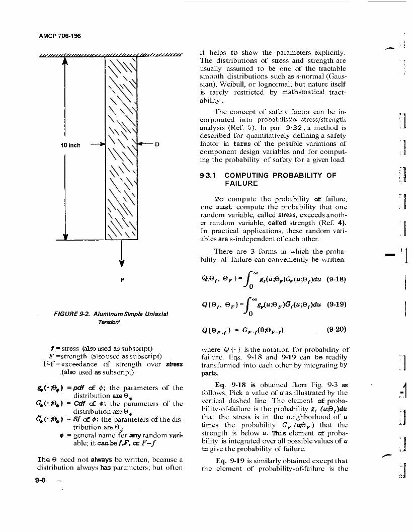
AMCP 706-196

//////////////////////////////■/////,

10 inch

//i»///////y////

V

P

FIGURE 9-2. Aluminum Simple Uniaxial Tension'

f = stress (also used as subscript) F =strength (also used as subscript)

F-f = exceedance of strength over stress (also used as subscript)

f*l>('&<tf) = pdf of #; the parameters of the distribution are©^

Qit>("'%) = Cdf of 4>', the parameters cf the distribution are ©^

^>(" >6^) - Sf o£ 4>; the parameters of the distribution are ©^

0 = general name for any random variable; it can bG f-f, or F—f

The © need not always be written, because a distribution always has parameters; but often

9-8

it helps to show the parameters explicitly. The distributions of stress and strength are usually assumed to be one of the tractable smooth distributions such as s-normal (Gaus- sian), Weibull, or lognormal; but nature itself is rarely restricted by mathematical tract- ability .

The concept of safety factor can be incorporated into probabilistic stress/strength analysis (Ref. 5). In par. 9-32, a method is described for quantitatively defining a safety factor in terms of the possible variations of component design variables and for computing the probability of safety for a given load.

9-3.1 COMPUTING PROBABILITY OF FAILURE

To compute the probability of failure, one must compute the probability that one random variable, called stress, exceeds another random variable, called strength (Ref. 4). In practical applications, these random variables are s-independent of each other.

There are 3 forms in which the probability of failure can conveniently be written.

Q{©,, ©F}= / 'g,{ü&r)C^(u#f)du (9-18)

Q{Gf, QF}= f°°gF(u&F)Gf(u;er)du (9-19)

Qi.eF.f} = GF_f(0&F.,) (9-20)

where Q {• ) is the notation for probability of failure. Eqs. 9-18 and 9-19 can be readily transformed into each other by integrating by parts.

Eq. 9-18 is obtained fkom Fig. 9-3 as follows, Pick a value of u as illustrated by the vertical dashed line. The element of probability-of-failure is the probability gf (uj&f)du that the stress is in the neighborhood of u times the probability GF (vrßF) that the strength is below u. This element of probability is integrated over all possible values of u to give the probability of failure.

Eq. 9-19 is similarly obtained except that the element of probability-of-failure is the

AMCP 706-196

<3j

9f gF

V 1

/ t-* k. N.

^-"t

FIGURE 9-3. Typical Probability Density Function g of Stresst and Strength F.

probability gF(u,QF)du that the strength is in the neighborhood of u times the probability Gf{uj9f) that the stress is above u.

Eq. 9-20 is derived by considering the distribution of F-f. GFf(u;@F _f) is the Cdf of F-f at the point u. The failure probability is the probability that F-f «* 0;fhis probability is GF f(0;QFf) by definition of the Cdf.

Even though it is possible to use any of the three equations 9-18, 9-19, 9-20 in a calculation, usually one will be much more tractable than the others.

The solution of practical problems requires the evaluation of an integral. For some stress and strength factors, these integrals can be expressed in terms of known functions. In other cases, the integrals must be numerically evaluated. Several practical cases are considered:

(1) s-Normally Distributed Strength and s-norntally Distributed Stress

Given:

(1) Stress f has s-normal (Gaussian) distribution with mean \if and standard deviation

(2) Strength F has s-normal (Gaussian) distribution with mean ßF and standard deviation oF.

(3) Stress and strength are s-independent, given that the parameters of their distributions are known.

Find: Probability of failure,

Solution: Eq. 9-20 is easiest to use because the distribution of F-f is easily calculated. If 2 random variables are s-independent-

ly and s-normally distributed, their difference has a s-normal distribution whose mean is the difference of the 2 means and whose variance is the sum of the 2 variances. (This statement is true regardless of the distributions, but the results are very tractable for the s-normal distribution.) Therefore F-f has a s-normal distribution with mean nFf

7 - n. (9-21)

and standard deviation o F-f

2\Vi 'Ff K + °f) (9-22)

The probability of failure Q is, from Eq. 9-20

Q = gauf [&£4- 'F-f

(9-23)

where gauf is the Cdf of the standard s-normal (Gaussian) distribution. (Named analogously to the error function.)


(2) Weibull Distributed Strength and Weibull Distributed Stress

The Weibull distribution is more difficult to work with than the s-normal distribution. The probability of failure cannot be obtained in closed form. The procedure used to compute the probability of failure for cases in which both stress and strength have Weibull distributions is to develop the integral expression for probability of failure and to evaluate this integral numerically. A detailed table of values of the integral for Weibull parameter values pertinent to mechanical problems is given in Ref. 6.

9-9

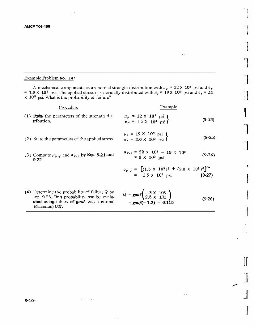
AMCP 706-196

Example Problem No. 14 :

A mechanical component has a s-normal strength distribution with pF = 22 X 103 psi and oF

= 1.5 X 103 psi. The applied stress is s-normally distributed with p( - 19 X 103 psi and af = 2.0 X 103 psi. What is the probability of failure?

Procedure Example

(1) State the parameters of the strength dis- nF - 11 X 103 psi ^ tribution. oF = 1.5 X 103 psi / (9"24)

Hf = 19 X 103 psi i (2) State the parameters of the applied stress. 0f = 2.0 X 103 psi / (9-25)

(3) Compute ßF_f and aF_, by Eqs. 9-21 and PF"' ~ l\X-,IT ~. 19 * 10* (9-26)

°F-r = li1-5 x 103)2 + <20 x 103)*JW

= 2.5 X 103 psi (9-27)

(4) Determine the probability cf failure Q by „ _ -/—3 X 103 \ Eq. 9-23, This probability can be evalu- ^"'ySTS X 103 ) (9-28) ated using tables cf gauf, viz., s-normal = gauf(— 1.2) = 0.115 (Gaussian) Cdf.

1 1

1

9-10-

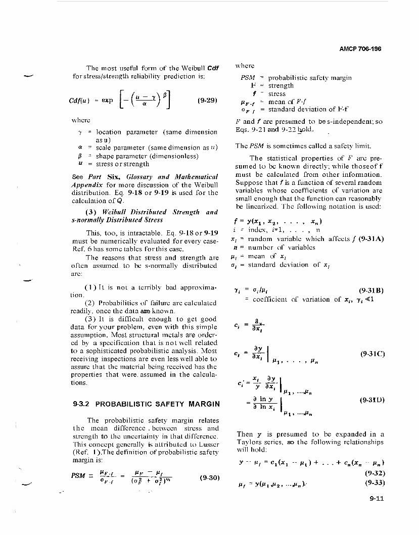
AMCP 706-196

The most useful form of the Weibull Cdf for stress/strength reliability prediction is:

Cdftu) = exp [~("-^y] (9-29)

where

a

ß u

location parameter (same dimension asu) scale parameter (same dimension as«) shape parameter (dimensionless) stress or strength

See Part Six, Glossary and Mathematical Appendix for more discussion of the Weibull distribution. Eq. 9-18 or 9-19 is used for the calculation of Q.

(3) Weibull Distributed Strength and s-normally Distributed Stress

This, too, is intractable. Eq. 9-18 or 9-19 must be numerically evaluated for every case- Ref. 6 has some tables forthis case.

The reasons that stress and strength are often assumed to be s-normally distributed are:

(l)It is not a terribly bad approximation.

(2) Probabilities of failure are calculated readily, once the data are known.

(3) It is difficult enough to get good data for your problem, even with this simple assumption. Most structural metals are ordered by a specification that is not well related to a sophisticated probabilistic analysis. Most receiving inspections are even less well able to assure that the material being received has the properties that were, assumed in the calculations.

9-3.2 PROBABILISTIC SAFETY MARGIN

The probabilistic safety margin relates the mean difference .between stress and strength to the uncertainty in that difference. This concept generally is attributed to Lusser (Ref. l)The definition of probabilistic safety margin is:

PSM s £fj£_ = >F-r {of. + o})* (9-30)

where

PSM = probabilistic safety margin F = strength f - stress

iiF.f = mean of F-f oFf = standard deviation of F-f

F and f are presumed to be s-independent; so Eqs. 9-21 and 9-22 Uold.

The PSM is sometimes called a safety limit.

The statistical properties of F are presumed to be known directly; while thoseof f must be calculated from other information. Suppose that f is a function of several random variables whose coefficients of variation are small enough that the function can reasonably be linearized. The following notation is used:

f = y(*X, *2» • - • . Xn) i - index, i-l, . . . , n

X; = random variable which affects / (9-31A) n = number of variables

Mf = mean of xi

a,. = standard deviation of x.

7, = o.Jn, (9-31B) = coefficient of variation of JC,-, ji <1

c =-!*- « a*,

c> = ay

' a*.. I fl\ » • • • » Mn

(9-31C)

c. = xt by y a*,

b In y 3 In X;

Hi y -,P„

**i. -J«„

(9-31D)

Then y is presumed to be expanded in a Taylors series, so the following relationships will hold:

y - ,if = c^*! - Mi) + • - • + cn(xn - /!„)

(9-32)

Vf = y(Mt^2- •-^n)' (9-33)

9-11

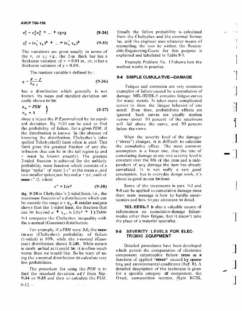
AMCP 706-196

a2, = c?a cm

7?=<Ci'7i>2 + - + (^7„)2

(9-34)

(9-35)

The variations are given usually in terms of the ot or 7;; e.g., the 2-in. thick bar has a thickness variation of a = 0.01 in., or, it has a thickness variation of y = 0.5%.

The random variable n defined by :

»? = •F-f

(9-36)

has a distribution which generally is not known. Its mean and standard deviation are easily shown to be:

M„ = PSM \

o„ =1 / (9-37)

since r\ is just the F-fîormalized by its standard deviation. Eq. 9-20 can be used to find the probability of failure, for a given PSM, if the distribution is known. In the absence of knowing the distribution, Chebyshev's (also spelled Tchebycheff) limit often is used. This limit gives the greatest fraction of any distribution that can be in the tail region (/J and a must be known exactly). The greatest 2-sided fraction is achieved for the unlikely probability mass function which consists of a large "spike" of mass 1-e* at the mean p , and two smaller spikes just beyond p ± 77 a, each of mass e * /2, where

e* =1/T?5 (9-38)

Eq. 9-38is Chebyshev's 2-sided limit, i.e., the maximum fraction of a distribution which can be outside the range ß ± TJ0 . A similar analysis shows that the 1-sided limit, the fraction that can be beyond p + r\0, is l/(n2 + l).Table

9-1 compares the Chebyshev inequality with the s-normal (Gaussian) distribution.

For example, if aPSM were 3.0, the maximum (Chebyshev) probability of failure (1-sided) is 10%, while the s-normal (Gaus- sian) distribution shows 0.14%. While nature is rarely as bad as it could be, it is often much worse than we would like. So be wary of using the s-normal distribution to calculate very low probabilities.

The procedure for using the PSM is to find the standard deviation off from Eqs. 9-34 or 9-35 and then to calculate the PSM.

Usually the failure probability is calculated from the Chebyshev and the s-normal formulas, arid the engineer uses whatever means of reconciling the two he wishes; the Reason- able-Engineering-Guess for this purpose is explained and tabulated in Table 9-1.

Example Problem No. method works in practice.

15 shows how the

9-4 SIMPLE CUMULATIVE-DAMAGE

Fatigue and corrosion are very common examples of failure caused by a cumulation of damage. MIL-HDBK-5 contains fatigue curves for many metals. It takes many complicated curves to show the fatigue behavior of one metal. Even then, probabilistic effects are ignored. Such curves are usually median curves—about 50 percent of the specimens will fail above the curve, and 50 percent below the curve.

When the severity level of the damager ("stress") changes, it is difficult to calculate the cumulative effect. The most common assumption is a linear one, that the rate of cumulating damage at any one severity level is constant over the life of the item and is independent of any damage the item has already cumulated. It is not really a very good assumption, but in everyday design work, it's about as good as can be done.

Some of the treatments in pars. 9-2 and 9-3 can be applied to cumulative damage since their main message is how to handle uncertainties and how to pay attention to detail.

MIL-HDBK-5 is also a valuable source of information on cumulative-damage failure- modes other than fatigue, but it doesn't take the place of a material specialist.

9-5 SEVERITY LEVELS FOR ELEC- TRONIC EQUIPMENT

Detailed procedures have been developed which permit the computation of electronic component catastrophic failure rates as a function of applied "stress" caused by operating and environmental conditions (Ref. 8). A detailed description of the technique is given for a specific category cf component, the fixed, composition resistor, Style RC22,

'I

9-12

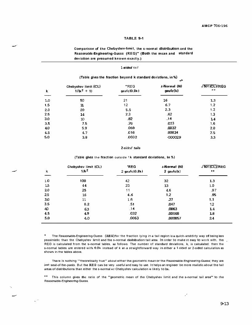
AMCP 706-196

TABLE 9-1

Comparison of the Chebyshev-limit, the s-normal distribution and the Reasonable-Engineering-Guess (REG)" (Both the mean and standard

deviation are presumed known exactly.)

1 sided tail

(Table gives the fraction beyond k standard deviations, in%)

Chebyshev limit {CU "REG sJMormal (N) JNX (CD/REG k 1/(k2 + 1) gaufc(0.8k) gaufc(k) **

1.0 50 21 16 1.3 1.5 31 12 6.7 1.2

2.0 20 5.5 2.3 1.2 2.5 14 2.3 .62 1.3 3.0 10 .82 .14 1.4 3.5 7.5 .26 .023 1.6 4.0 5.9 .069 .0032 2.0 4.5 4.7 .016 .00034 2.5 5.0 3.8 .0032

2-sided tails

-000029 3.3

(Table gives the fraction outside ±k standard deviations, in %)

Chebyshev limit (CD ■REG s-Normal (N) 7NX<CL)/REG k 1/k2 2 gaufc(0.8k) 2 gaufc(k) »»

1.0 100 42 32 1.3 L5 44 23 13 1.0 2.0 25 11 4.6 .97 2.5 16 4.6 1.2 .95 3.0 11 1.6 .27 1.1 3.5 8.2 .51 .047 1.2 4.0 6.3 .14 .0063 1.4 4.5 4.9 .032 .00068 1.8 5.0 4.0 .0063 .000057 2.4

* The Reasonable-Engineering-Guess (REG)for the fraction lying in a tail region isa quick-anddirty way of being less pessimistic than the Chebyshev limit and the s-normal distribution tail area. In order to make it easy to work with, the REG is calculated from the s-normal tables, as follows. The number of standard deviations, k, is calculated; then the s-normal tables are entered with 0.8k instead of k in a straightforward way in either a 1-sided or 2-sided calculation as shown in the tables above.

There is nothing "theoretically true" about either the geometric mean or the Reasonable-Engineering-Guess; they are just seat-of-the-pants. But the REG can be very useful and easy to use. It helpsan engineer be more realistic about the tail areas of distributions than either the s-normal or Chebyshev calculation is likely to be.

" This column gives the ratio of the Reasonable-Engineering-Guess.

'geometric mean of the Chebyshev limit and the s-normal tail area" to the

9-13

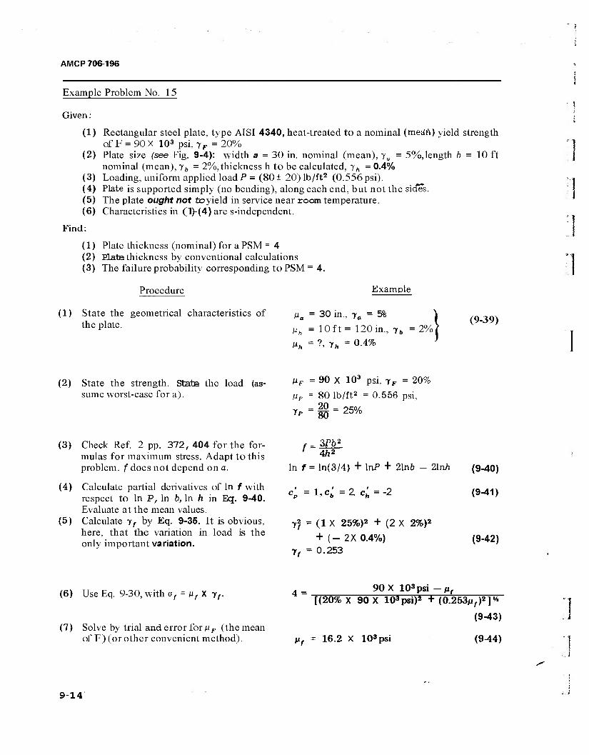
AMCP 706-196


Given :

(1) Rectangular steel plate, type AISI 4340, heat-treated to a nominal (mean) yield strength of F = 90 X 103 psi, yF = 20%

(2) Plate size (see Fig. 9-4): width a = 30 in. nominal (mean), ya = 5%,length b = 10 ft nominal (mean), 7b = 2%,thickness h to be calculated, yh = 0.4%

(3) Loading, uniform applied load P = (80 ± 20) lb/ft2 (0.556 psi). (4) Plate is supported simply (no bending), along each end, but not the sides. (5) The plate ought not to yield in service near room temperature. (6) Characteristics in (l)-(4) are s-independent.

Find:

(1) Plate thickness (nominal) for a PSM = 4 (2) Plate thickness by conventional calculations (3) The failure probability corresponding to PSM = 4.

Procedure ExamDle

(1) State the geometrical characteristics of the plate.

Ha = 30 in., 70 = 5% |

Ub = 10ft = 120 in., yb = 2%,

ßh = ?. 7„ = 0.4% '

(9-39)

(2) State the strength. State the load (assume worst-case for a).

MF = 90 X 103 psi, yF = 20%

UH = 80 lb/ft2 = 0.556 psi. 20 _ SO 25%

(3) Check Ref. 2 pp. 372, 404 for the formulas for maximum stress. Adapt to this problem, f does not depend on a.

(4) Calculate partial derivatives of In f with respect to In P, In b, In h in Eq. 9-40. Evaluate at the mean values.

(5) Calculate yf by Eq. 9-35. It is obvious, here, that the variation in load is the only important variation.

f _ 3F52

' Ah2

In f = ln(3/4) + InP + 21n6 - 21n/i (9-40)

c'p =l,c'=Z c'h=-2 (9-41)

7, = (1 X 25%)2 + (2 X 2%)2

+ (-2X0.4%) (9-42) yf = 0.253

(6) Use Eq. 9-30, with of = pfX yf.

(7) Solve by trial and error for nF (the mean of F) (or other convenient method).

4 = 90 X 103psi-fi, [(20% X 90 X 103psi)2 + (0.253/i,.)2]*

(9-43)

It, = 16.2 X 103psi (9-44)

9-14 ;..j

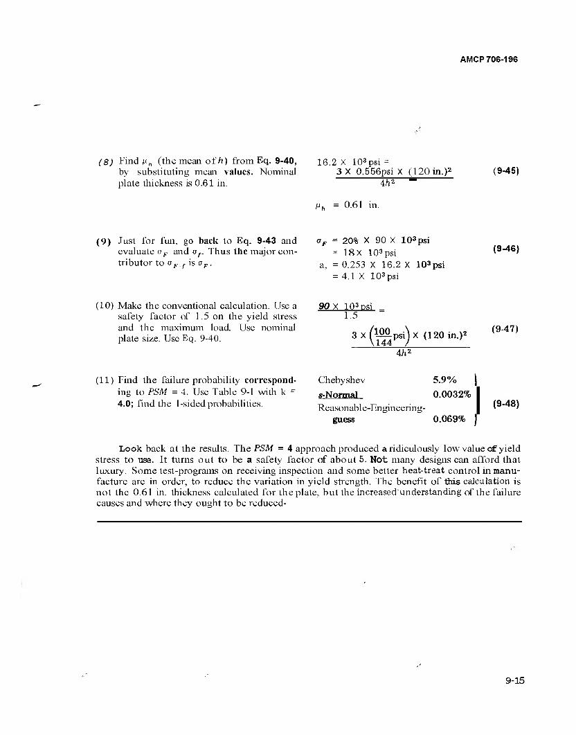
AMCP 706-196

(8) Find/ih (the mean of h) from Eq. 9-40, by substituting mean values. Nominal plate thickness is 0.61 in.

16.2 X 103psi = 3X 0.556psi X (120 in.)2

4/i2 _

UL = 0.61 in.

(9-45)

(9) Just for fun, go back to Eq. 9-43 and aF = 20% X 90 X 103psi evaluate oF and af. Thus the major con- = 18X 103psi '■'■'-'--■■■ ,d= 0.253 X 16.2 X 103psi

= 4.1 X 103psi

(9-46)

tributor to o F f is a F

(10) Make the conventional calculation. Use a safety factor of 1.5 on the yield stress and the maximum load. Use nominal plate size. Use Eq. 9-40.

90 X 103psi _ 1.5

3 X GS-) X (120 in.)2 (9-47)

4/i5

(11) Find the failure probability corresponding to PSM =4. Use Table 9-1 with k = 4.0; find the 1-sided probabilities.

Chebyshev 5.9% )

s-Normal 0.0032% Reasonabl e-Engineering-

guess 0.069%

(9-48)

Look back at the results. The PSM = 4 approach produced a ridiculously low value of yield stress to use. It turns out to be a safety factor of about 5. Not many designs can afford that luxury. Some test-programs on receiving inspection and some better heat-treat control in manufacture are in order, to reduce the variation in yield strength. The benefit of this calculation is not the 0.61 in. thickness calculated for the plate, but the increased'understanding of the failure causes and where they ought to be reduced-

9-15

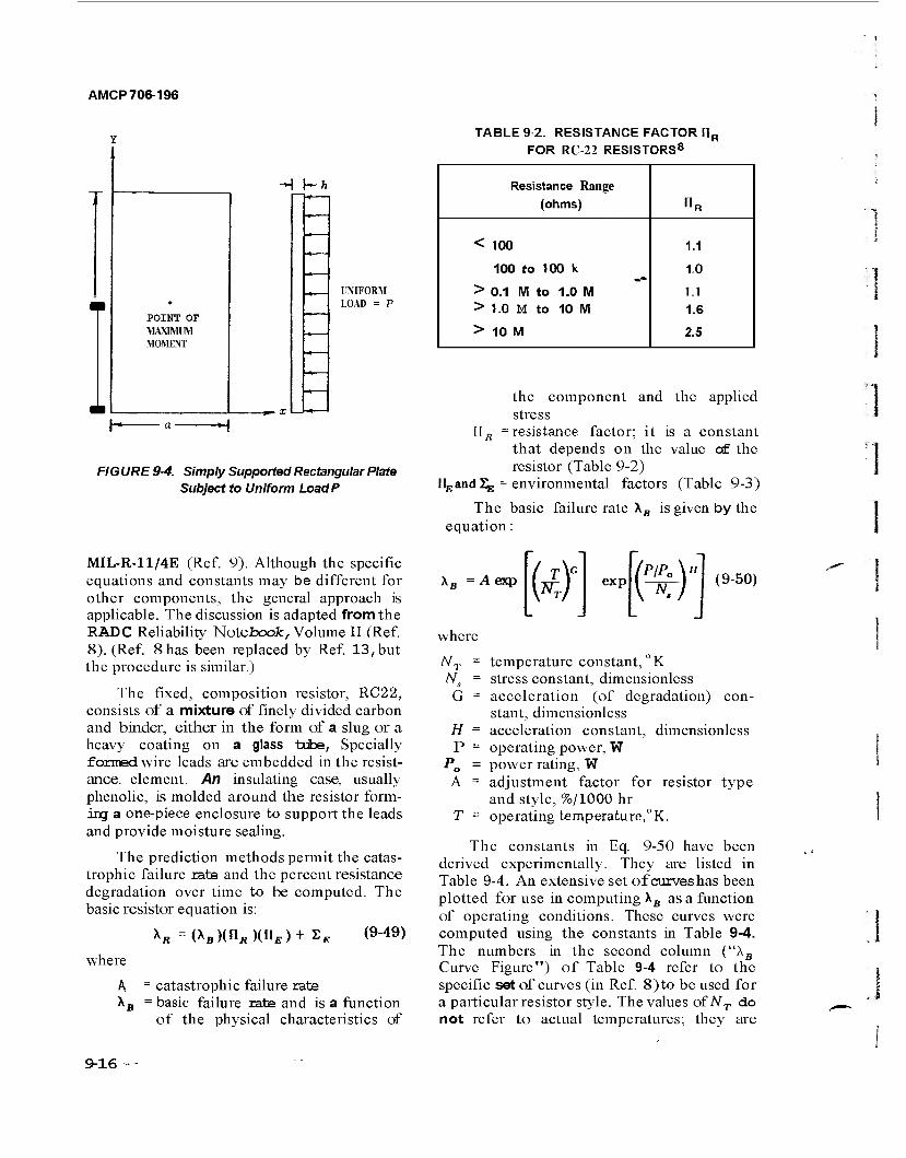
AMCP706-196

POINT OF MAXIMUM MOMENT

UNIFORM UOAD = P

FIG URE 9-4. Simply Supported Rectangular Plate Subject to Uniform LoadP

TABLE 9 2. RESISTANCE FACTOR nf

FOR RC-22 RESISTORS8

Resistance Range (ohms) «R

< 100 1.1

100 to 100 k 1.0

> 0.1 M to 1.0 M 1.1 > 1.0 M to 10 M 1.6

> 10 M 2.5

IIEand^

the component and the applied stress

: resistance factor; it is a constant that depends on the value of the resistor (Table 9-2) environmental factors (Table 9-3)

The basic failure rate \B is given by the equation:

MIL-R-11/4E (Ref. 9). Although the specific equations and constants may be different for other components, the general approach is applicable. The discussion is adapted from the RADC Reliability 'Notebook, Volume II (Ref. 8). (Ref. 8 has been replaced by Ref. 13, but the procedure is similar.)

The fixed, composition resistor, RC22, consists of a mixture of finely divided carbon and binder, either in the form of a slug or a heavy coating on a glass tube, Specially formed wire leads are embedded in the resistance, element. An insulating case, usually phenolic, is molded around the resistor forming a one-piece enclosure to support the leads and provide moisture sealing.

The prediction methods permit the catastrophic failure rate and the percent resistance degradation over time to be computed. The basic resistor equation is:

(9-49)

where

A A»

x« =(*B)(nÄ)(n£)+££

= catastrophic failure rate = basic failure rate and is a function

of the physical characteristics of

\B = A exp [N-r) «P {-RT) (9-50)

where

NT = N. =

H = P =

P„ = A =

T =

temperature constant, ° K stress constant, dimensionless acceleration (of degradation) constant, dimensionless acceleration constant, dimensionless operating power, W power rating, W adjustment factor for resistor type and style, %/1000 hr operating temperature,0K.

The constants in Eq. 9-50 have been derived experimentally. They are listed in Table 9-4. An extensive set of curves has been plotted for use in computing \B as a function of operating conditions. These curves were computed using the constants in Table 9-4. The numbers in the second column ("AB

Curve Figure") of Table 9-4 refer to the specific set of curves (in Ref. 8) to be used for a particular resistor style. The values o£NT do not refer to actual temperatures; they are

9-16

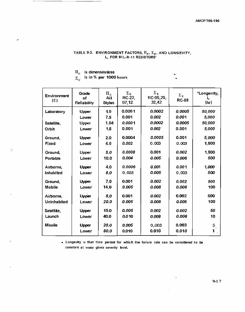
AMCP 706-196

TABLE 9-3. ENVIRONMENT FACTORS, nE, £E, AND LONGEVITY, L, FOR MIL-R-11 RESISTORS'

n. is dimensionless £ is in % per 1000 hours

Environment <E)

Grade of

Reliability

nK All

Styles

SE RC-22. 07,12

RC-05,20, 32,42

2K RC-08

*Longevity, L

(hr)

Laboratory Upper 1.0 0.0001 0.0002 0.0005 50,000

Lower 7.5 0.001 0.002 0.001 5,000

Satellite, Upper 1.04 0.0001 0.0002 0.0005 50,000

Orbit Lower 1.5 0.001 0.002 0.001 5,000

Ground, Upper 2.0 0.0004 0.0005 0.001 5,000

Fixed Lower 4.0 0.002 0.003 0.003 1,500

Ground, Upper 5.0 0.0008 0.001 0.002 1,500

Portable Lower 10.0 0.004 0.005 0.006 500

Airborne, Upper 4.0 0.0006 0.001 0.001 1,000

Inhabited Lower 8.0 0.003 0.005 0.003 500

Ground, Upper 7.0 0.001 0.002 0.002 500

Mobile Lower 14.0 0.005 0.008 0.006 100

Airborne, Upper 8.0 0.001 0.002 0.002 500

Uninhabited Lower 20.0 0.005 0.008 0.006 100

Satellite, Upper 15.0 0.005 0.002 0.002 50

Launch Lower 40.0 0.010 0.008 0.006 10

Missile Upper 20.0 0.005 0,003 0.003 5

Lower 80.0 0.010 0.010 0.010 1

• Longevity is that time period for which the failure rate can be considered to be

constant at some given severity level.

9-17

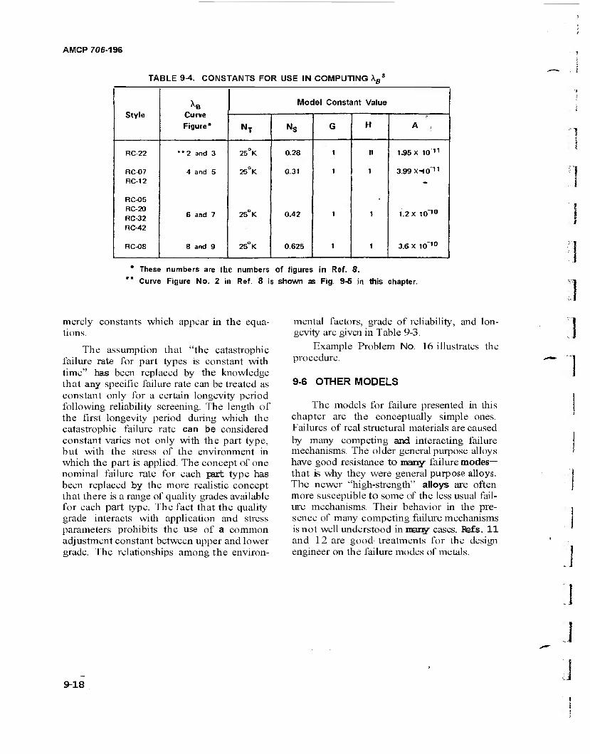
AMCP 706-196

TABLE 9-4. CONSTANTS FOR USE IN COMPUTING \B8

Style *B

Curve Figure*

Model Constant Value

NT NS G H A ,

RC-22

RC-07 RC-12

RC-05 RC-20 RC-32 RC-42

RC-08

"2 and 3

4 and 5

6 and 7

8 and 9

25° K

25°K

25° K

25° K

0.28

0.3»

0.42

0.625

1

1

1

1

n

i

1

1

155 X in"'1

3.99 X10~11

1.2 X 10~10

3.6 X 10~10

* These numbers are the numbers of figures in Ref. 8. Curve Figure No. 2 in Ref. 8 is shown as Fig. 9-5 in this chapter.

merely constants which appear in the equations.

The assumption that "the catastrophic failure rate for part types is constant with time" has been replaced by the knowledge that any specific failure rate can be treated as constant only for a certain longevity period following reliability screening. The length of the first longevity period during which the catastrophic failure rate can be considered constant varies not only with the part type, but with the stress of the environment in which the part is applied. The concept of one nominal failure rate for each part type has been replaced by the more realistic concept that there is a range of quality grades available for each part type. The fact that the quality grade interacts with application and stress parameters prohibits the use of a common adjustment constant between upper and lower grade. The relationships among the environ-

mental factors, grade of reliability, and longevity are given in Table 9-3.


9-6 OTHER MODELS

The models for failure presented in this chapter are the conceptually simple ones. Failures of real structural materials are caused by many competing and interacting failure mechanisms. The older general purpose alloys have good resistance to many failure modes— that is why they were general purpose alloys. The newer "high-strength" alloys are often more susceptible to some of the less usual failure mechanisms. Their behavior in the presence of many competing failure mechanisms is not well understood in many cases. Eefs. 11 and 12 are good- treatments for the design engineer on the failure modes of metals.

9-18

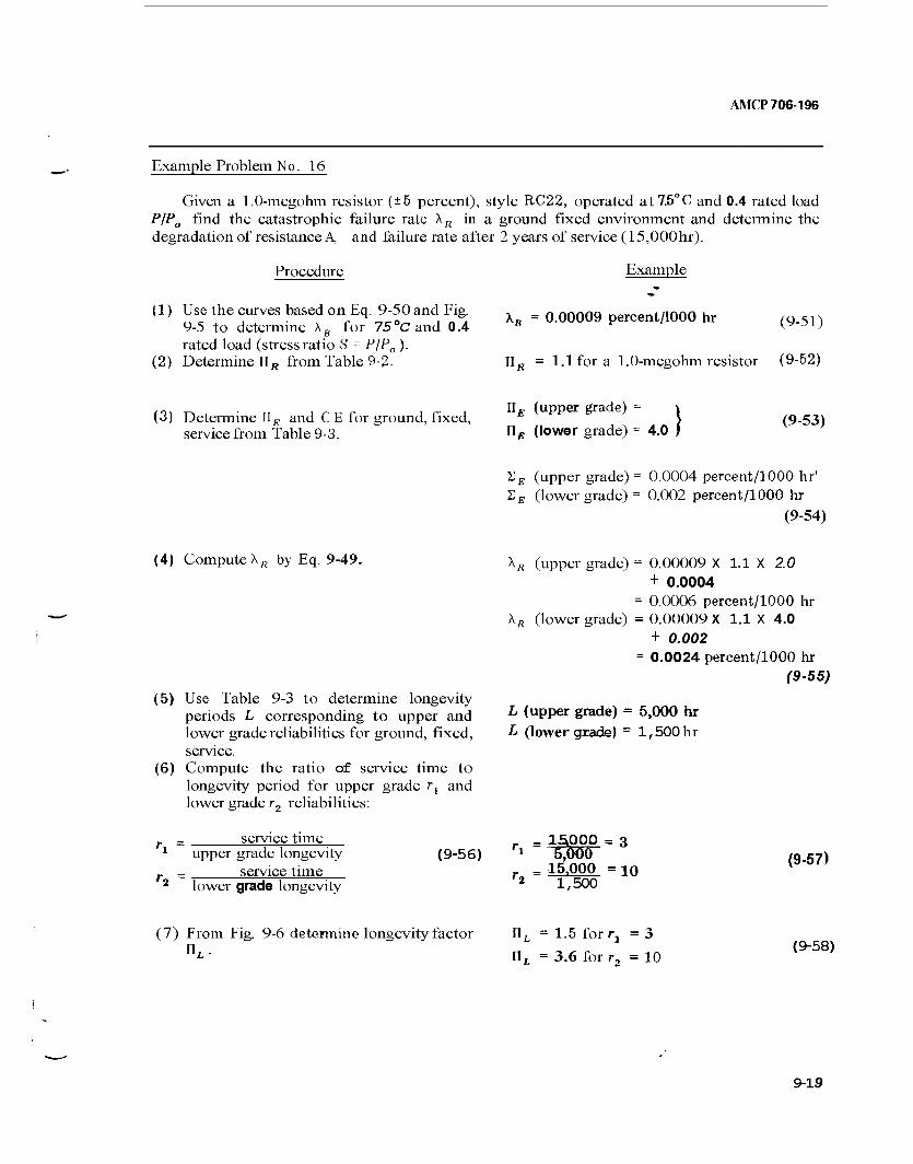
AMCP 706-196


Given a 1.0-megohm resistor (±5 percent), style RC22, operated at7,5°C and 0.4 rated load P/P0 find the catastrophic failure rate AR in a ground fixed environment and determine the degradation of resistance A, and failure rate after 2 years of service (15,000hr).

Procedure Example

(1) Use the curves based on Eq. 9-50 and Fig. 9-5 to determine XB for 75°C and 0.4 rated load (stress ratio S = PjPl} ).

(2) Determine nR from Table 9-2-

\B = 0.00009 percent/1000 hr (9-51)

II fi = 1.1 for a 1.0-megohm resistor (9-52)

(3) Determine UB and CE for ground, fixed, service from Table 9-3.

II^ (upper grade) =

nB (lower grade) = 4.0 (9-53)

ZE (upper grade) = 0.0004 percent/1000 hr' S£ (lower grade) = 0.002 percent/1000 hr

(9-54)

(4) Compute XR by Eq. 9-49.

(5) Use Table 9-3 to determine longevity periods L corresponding to upper and lower grade reliabilities for ground, fixed, service.

(6) Compute the ratio of service time to longevity period for upper grade rl and lower grade r2 reliabilities:

\R (upper grade) = 0.00009 X 1.1 X 2.0 + 0.0004

= 0.0006 percent/1000 hr \R (lower grade) = 0.00009 X 1.1 X 4.0

+ 0.002 = 0.0024 percent/1000 hr

(9-55)

L (upper grade) = 5,000 hr

L (lower grade) = l,500hr

r service time 1 upper grade longevity

r service time 2 lower grade longevity

r =150pp_=3 (9-56) * 5,000

. = 15,000 = io 2 1,500

(9-57)

(7) From Fig. 9-6 determine longevity factor n,.

nL = 1.5 forr, =3

nL = 3.6 for r2 = 10 (9-58)

9-19

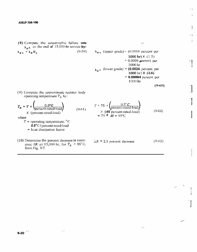
AMCP 706-196

(8) Compute X

X

the catastrophic failure rate

VR L = X

at the end cf 15,000-hr service by:

RIlL (9-59)

(9) Compute the approximate resistor body operating temperature TB by:

TB =T + C 0.5"C percent-rated-load/

X (percent-rated-load)

where T = operating temperature, ° C

0.5" C/(percent-rated-load = heat dissipation factor

(9-61)

lR L

\RL

(upper grade)

(lower grade)

(0.0006 percent per

1000 hr)X (1.5) 0.0009 percent per 1000 hr (0.0024 percent per 1000 hr) X (3.6) 0.00864 percent per 1000 m-

(9-60)

T ./ 0.5" C \percent-rated-loady

75+1 u.yu \ \percent-rated-loady

X (40 percent-rated-load) = 75 + 20 = 95°C

(9-62)

(10) Determine the percent decrease in resistance AR at 15,000 hr, for TB = 95° C, from Fig. 9-7.

Ai? - 2.5 percent decrease (9-63)

9-20

AMCP 706-196

0.01

0.007 - 1

ISOTHERM

1 0.005 0.004

0.003 - TEMPE °C 150

RATURf -•T- r

0.002

- 100 J 0.001

0.0007

0.0005 0.0004

0.0003

50-r 0.0002

0.00007 S Oy^

O.O0004

0.00003

r i s

/i / 1 /

0.00002

0.2 0.4 0.6 0.8 1.0 1.2

STRESS RATIO, S

P OPERATING POW RATED POWE

WER\

FIGURE 9-5. Determination of Failure Rate XB

as Related to Stress Ratio S for MIL-R-11/4E Resistors, RC-22'

"L

.____ _ — —.— . '"" — """ — — __ _ v CARBON COMP< 3S*TION in :i

^

—"l

50

MULTIPLESOF LONGEVITY

FIGURE 9-6. Determination of Longevity Factor irL for MIL-R-II Resistors, All Styles'

1.000,000

100.000

3 O 10.000

ID

f

a

\\

^ ^

PERCE OECRE

NT ASE AF i» 2.5 \ 5 \J0 \2S> N.30

\:

\ 25 50 75 100 125 150 175 200

BODY TEMPERATURE Te."C

FIGURE 9-7- Determination of Resistor Longevity as Related to Body Temperature, for MIL-R-11 Re-

sistors, All Styles'

9-21

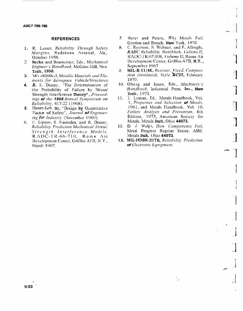
AMCP 706-196

REFERENCES

R Lusser, Reliability Through Safety Margins, Redstone Arsenal, Ala., October 1958. Marks and Baumeister, Eds., Mechanical Engineer's Handbook, McGraw-Hill, New York,1958. MIL-HDBK-5,Metallic Materials and Ele- ments for Aerospace Vehicle Structures. R. L. Disney, "The Determination of the Probability of Failure by Stress/ Strength Interference Theory", Proceed- ings of the 1968Annual Symposium on Reliability, 417-22 (1968). Hsuan-Loh Sc, "Design by Quantitative Factor of Safety", Journal of Engineer- ing for Industry (November 1960). C. Lipson, S. Narendra, and R. Disney, Reliability Prediction Mechanical Stress/ Strength Interference Models, R ADC-TR-66-710, Rome Air Development Center, Griffiss AFB, N. Y., March 1967.

8.

9.

10.

11.

12.

13.

Barer and Peters, Why Metals Fail, Gordon and Breach, New York, 1970. C. Ryerson, S. Webster, and F. Albright, RADC Reliability Notebook, VolumeII, RADC-TR-67-108, Volume 11, Rome Air Development Center, Griffiss AFB, N.Y., September 1967. MIL-R-11/4E, Resistor, Fixed, Composi- tion (insulated), Style ^RC22, February 1970. Oberg and Jones, Eds., Machinery's Handbook, Industrial Press, Inc., New York. 1971. T. Lyman, Ed., Metals Handbook, Vol. 1, Properties and Selection of Metals, 1961, and Metals Handbook, Vol. 10, Failure Analysis and Prevention, 8th Edition, 1975, American Society for Metals, Metals Park, Ohio 44073. D. J. Wulpi, How Components Fail, Metal Progress Reprint Series, ASM, Metals Park. Ohio 44073. MIL-HDBK-217B, Reliability Prediction of Electronic Equipment.

1

9-22 J

AMCP 706-196

CHAPTER 10 PARAMETER VARIATION ANALYSIS

10-0 LIST OF SYMBOLS

A/i

capacitance Cumulative distribution function Covariance of frequency fraction, in cell / number of standard deviations inductance number of cells, par. 10-3 number of units or characteristics subscript, implies nominal value, see Eq. 10-11 random variable, characteristic of apart mean of P, sometimes used with subscripts probability density function characteristic j tolerance limits for P probabilistic safety margin Resistance, par. 10-3 mean Resistance, par. 10-3 Resistance at center of cell i, par. 10-3

REG = Reasonable-Engineering- Guess sensitivity coefficients, see Eqs. 10-12,10-13 tolerance limit Variance of performance characteristic /' a function coefficient of variation of Vi, see Eq. 10-25 coefficient of variation of Pj, seeEq. 10-25 frequency change maximum A, standard deviation (often used with a subscript) standard deviation of Vt

Cdf =

cov = f =

/,- = k =

L = N = n =

o =

P =

P =

Pdf =

Pi =

P P rM IN >rM A X PSM =

R = R =

R.. =

S»£ii

Tf = Var =

Vi = y =

y'i -

7y =

Af =

m ax a =

10-1 INTRODUCTION

Parameter variation analysis, sometimes 'referred to as variability analysis, consists of a

useful set of tools for designing reliable systems. Through the use of these tools, the effects of variations of individual design parameters on system performance and reliability can be determined. The techniques need not be statistical. Ref. 18 is a good discussion of parameter variation analysis; it is written for practical use by engineers.

The worst-case method of variability analysis is a nonstatistical approach (Ref. 18) that can be used to determine whether it is possible, with given parameter tolerance limits, for the system performance characteristics to fall outside specifications. The answer is obtained by using system models in which parameters are set at either their upper or lower tolerance limits. Parameter values are chosen to cause each performance characteristic to assume first its maximum and then its minimum expected value. If these performance-characteristic values fell within specifications, the designer can be sure that the system has high drift reliability. If specifications are exceeded, drift-type failures are possible, but the probability of their occurrence remains unknown.

Statistics is combined with system analysis techniques in the moment method to estimate the probability that performance vaH. remain within specified limits (Ref. 18). The method applies the propagation-of-variance formula to the first two moments of component-part frequency distributions to obtain the moments of performance-characteristic frequency distributions. On the basis of this information, the probability that specific system parameters drift out of their acceptable range or drift reliability can be computed.

In the Monte Carlo method a large number of alternate replicas of a system are simulated by mathematical models (Ref. 18). Component values are selected randomly, and the performance of each replica is determined for its particular set of components. The perfonnance of the replicas are compared with specification limits to yield an accurate estimate of system reliability.

10-1

AMCP 706-196

Each of these methods and the basic mathematical theory of parameter variation analysis are discussed in the paragraphs that follow.

The fundamental approach in each method involves the systematic manipulation of a suitably arranged system model to give the desired information. All depend on the speed and accuracy afforded by the modem digital computer to manipulate the model and to process the data resulting from this manipulation.

The nonstatistical, worst-case approach is designed to give basic information concerning the sensitivity of a configuration to variability in the parameters of its component parts. This infomation is useful to the designer in selecting economical but adequately stable components for the circuit and in modifying the configuration to reduce the critical effects of certain parameters, On the other hand, the moment and Monte Carlo methods, which are statistical, use actual parameter-variability data to simulate real-life situations and predict the probability that performance is inside tolerance specifications. The moment method prediction of performance variability is usually less accurate than the Monte Carlo method, but still adequate for most purposes. The moment method provides information that is extremely useful to the designer in pinpoint- ing sensitive areas and reducing this sensitivity to parameter variability,

In addition to providing data on drift- type failures, the techniques are all capable of giving "stress level" information of the type needed for estimating catastrophic-failure rates. They are useful, powerful tools for predicting overall reliability.

10-2 DESCRIPTIONSOFVARIABILITY

The performance of a system depends on the parameters of its component parts and on the particular set of values assigned to those parameters. Since these parameter values vary because of imperfect parts and environmental effects, system perfonnance variability is inevitable. This concept is illustrated in Fig. 10-1, where a performance characteristic V of a system is plotted as a function of parameter

P. V might represent the voltage or pressure at some point in the system, and P might represent the resistance of a resistor or the diameter of a nozzle.

Data for a plot of this type can be obtained by holding all parameters and environmental conditions, except P, constant at nominal values while P is varied over a range above and below its nominal-âlue. The nominal value of P falls at the point on the curve V = f(P) at which V = Vn om the design center. This curve describes the relationshp between V and P. When actual component, parts are obtained for the system, the values of P are found to lie, not exactly at P, but in the range indicated in the lower frequency distribution. The effect on V of this variability in P can be determined by projecting the P distribution up to the curve V = f(P) and over to the V axis. If the curve is essentially linear, the distribution of V will have basically the same shape as the distribution of P. Similarly, if the curve is highly nonlinear in the range of interest, the distribution of V will be a distorted version ofthat of P.

This concept of performance variability is understood readily on a parameter-by- parameter basis, and it can be handledeasily, in this manner, by the designer. What really is needed, however, is a means of handling real-life situations such as that shown in Fig. 10-2, where performance variability is influenced by several parameters simultaneously. Comparison of the functional relationships shows a positive correspondence between V, P1 , and Pz, and a negative correspondence between V and P2. V depends highly on P1

and P2, but only slightly on P3. The net variability of the performance characteristic V is influenced by all three parameters, and the contribution of each is a function of its importance in determining the value of V, as well as its own Variability.

All of the probability density functions (referred to as frequency distributions in Fig. 10-2) have an area of unity, regardless of shape. This means, of course, that those with a narrow base (low variability) have relatively greater height (high relative frequency). The 3-variable pdf of performance characteristic V has a broader base than any of the 1-variable

10-2

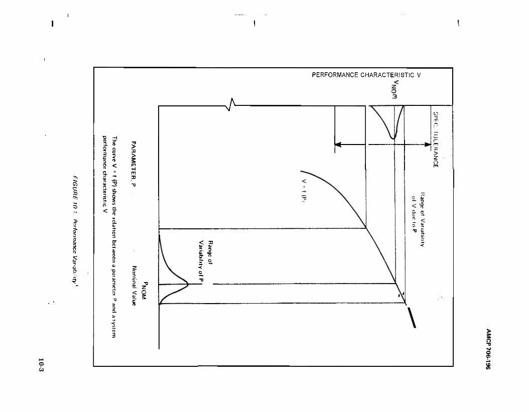
PERFORMANCE CHARACTERISTIC V

C5

3 Cu

5

■o H 3" "ü

0 > -S c 3 3 cu 3

< re

> O n < m

H 3- QJ

-♦» m 3

5 -D (/i 3*

u*

ö' Wl **

< 7 n>

2.

5 3 O" (ti

n>

3 DJ Z X) 0

3

3 5'

<

■o ID Z

o V c

2 m ts 3 a

■sA

< 3 eu tu

< o

01 -a

m x > 2 o m

o

3 es

- <

© I

CO

> S o ■o -J o 9

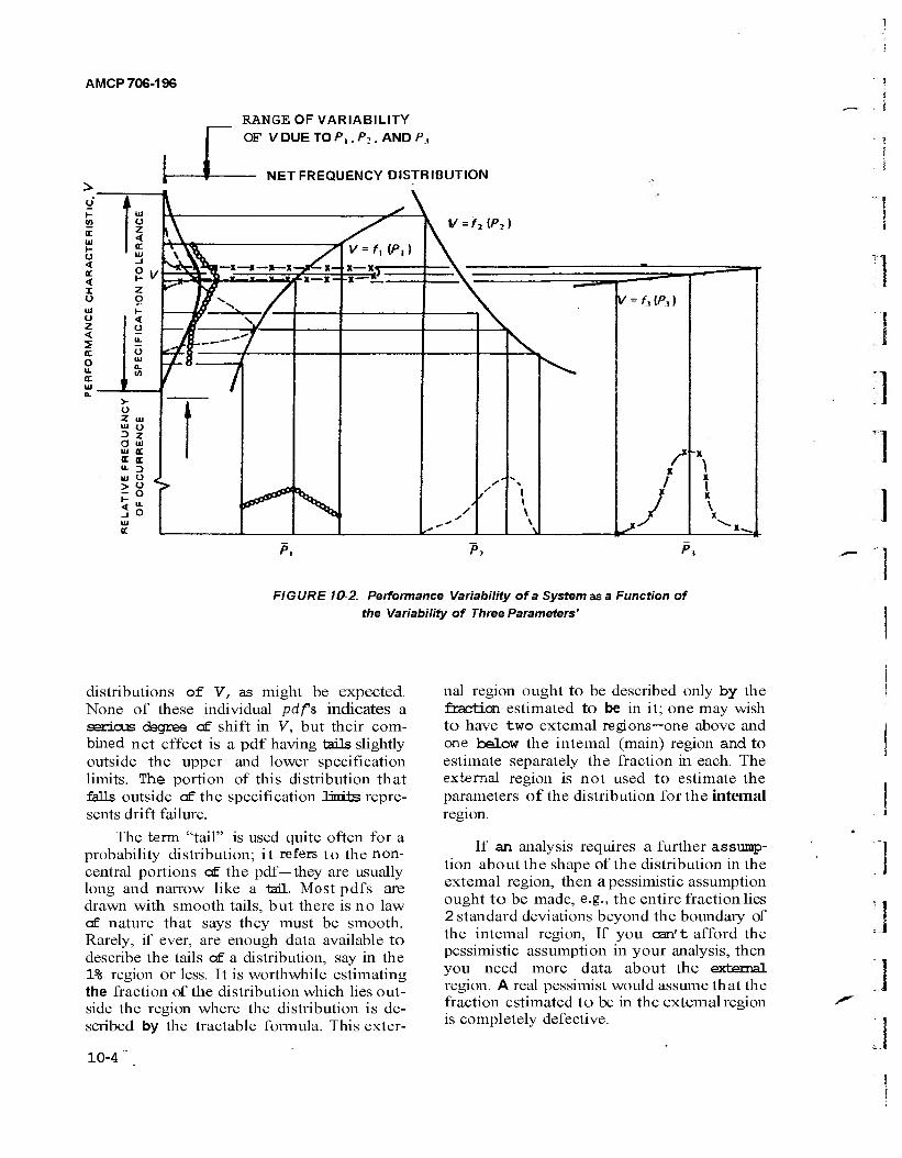
AMCP 706-196

01

O < < I o 111 o z < 2 cc o

L RANGE OF VARIABILITY OF V DUE TO />,. />;. AND A\,

NET FREQUENCY DISTRIBUTION

J i ui u z < cc ui

i\ ^ V = f2iP7)

\ V = fy (/>, ) \

z

AÄ»— * —* —*—* -y£-x— * XJT F*"

"4—ji «-»■»»»t £%—X — -x—!T. \" — 1

o If^ / V**f*Ws) < t? "\ / o u. 9 ~****7 o UI a. n

' ' >- u Z ui , ui o 3 Z 0 ui UI IE or cc

x \ UI O <» > o *> x' \ 1 X

I

5" J o ^ \

j

/ / I

i \ J X

\ X

u a

1 t^.

\ \ s' 1 -^1 -

p,

FIGURE 10-2. Performance Variability of a System as a Function of the Variability of Three Parameters'

1

distributions of V, as might be expected. None of these individual pdf s indicates a serious degree of shift in V, but their combined net effect is a pdf having tails slightly outside the upper and lower specification limits. The portion of this distribution that falls outside cf the specification unite represents drift failure.

The term "tail" is used quite often for a probability distribution; it refers to the non- central portions of the pdf—they are usually long and narrow like a tail. Most pdfs are drawn with smooth tails, but there is no law of nature that says they must be smooth. Rarely, if ever, are enough data available to describe the tails of a distribution, say in the 1% region or less. It is worthwhile estimating the fraction of the distribution which lies outside the region where the distribution is described by the tractable formula. This exter-

nal region ought to be described only by the fraction estimated to be in it; one may wish to have two external regions—one above and one below the internal (main) region and to estimate separately the fraction in each. The external region is not used to estimate the parameters of the distribution for the internal region.

If an analysis requires a further assumption about the shape of the distribution in the external region, then a pessimistic assumption ought to be made, e.g., the entire fraction lies 2 standard deviations beyond the boundary of the internal region, If you can't afford the pessimistic assumption in your analysis, then you need more data about the external region. A real pessimist would assume that the fraction estimated to be in the external region is completely defective.

10-4

AMCP 706-196

500

o --

Fre si. ency histogram

pdf {P}

r 900 940 980 I020 1060 "00 Resistonce. ohms

FIGURE 10-3. Frequency Histogram and Cumulative Polygon for a Typical Frequency

Distribution'

10-3 SOURCES OF VARIABILITY

In any sample group of similar components that have passed successfully through the production and inspection process (for example, 500, 10%, 1000-ohm resistors), many units will have nearly nominal resistance, some will have resistance values near the tolerance limits, and a few might have values outside of the tolerance limits. The distribution of resistance values is important because it can affect circuit performance variability.

The frequency histogram and the cumulative polygon provide a method of visualizing the distribution of resistance values. The histogram is formed by dividing the tolerance range (e.g., 900 to 1100 ohms) into a number of cells. In Fig. 10-3, 20-ohm cells are used. The column height for each cell is determined by the number of resistors whose values fall within the cell; it is an approximation to the pdf. The cumulative polygon is formed by cumulatively adding the number of resistors in each cell; it is an approximation to the Cdf. Relative frequency of occurrence is the frequency of occurrence divided by the total number of observations (500in this case).

A smooth frequency distribution (Fig. 10-4) can be obtained by fitting a curve to the histogram. The discussion that follows presumes that the sample was "infinitely" large; so that the smooth curve really does accur-

Parameter P

FIGURE 10-4. Moments of a Distribution'

ately represent the whole population. The first moment of the distribution is its mean value P, and is taken from the origin:

P X pdf{P}dP (10-1)

The first moment corresponds to the center of gravity of a plane area. The sum of first moments about the mean is zero, since positive and negative moments balance:

fPmi

0=/ (P J p rmin

(P - P) X pdf {P}dP (10-2)

The second central moment, i.e., (taken about the mean) is called the variance of :

of =f Jo

(P _ p)2X pdf {P}dP (10-3)

The variance corresponds directly to the moment of inertia of a plane area. The variance and its square root, the standard deviation op, are both used as measures of variability. Higher moments of a distribution are sometimes useful in defining skewness, peakedness, etc. If the distribution is s-normal (or any other that has no more than 2 parameters), only the first two moments are needed to determine its parameters.

10-5

AMCP 70^196

First and second moments of the sample can be calculated directly from the histogram if it is assumed that within each cell all component values occur at the midpoint of the cell or if the usual correction for grouping is used.


When a single component has several important parameters, there may be relationships among the parameter distributions. For example, for a semiconductor diode with a given offset voltage VD and dynamic resistance R„ some internal physical relationship may define a value or range of values for RD

with respect to VD . Another example can be given for a solid fuel rocket motor. The static pressure in the chamber is a function of fuel grain density, burning index, nozzle area, and bum surface area of the grain. Varying these parameters causes variations in chamber pressure, which can lead to unacceptable performance. Thus variations in the design parameters of a particular system can depend upon each other. The extent of direction of the linear component of the dependence, called the linear correlation, can be computed for the sample from:

if. PaJ ~ Fo)(PbJ ~ ?b) P =

■ PI o„o

(10-9) a"b

where

P = linear-correlation coefficient n = number of individual units tested

âj'^bj = measurements of parameters Pa

andPb on unitj a

a>°b = standard deviations for parameters Pa andPb

The linear-correlation coefficient p lies between +1 and —1. If the linear-correlation coefficient is negative, increases in one parameter correspond to decreases in the other. If the linear-correlation coefficient is positive, increases in one parameter correspond to increases in the other. The statistical literature usually uses the term correlation rather than linear-correlation for this concept. But since an engineer tends to think of correlation and dependence as synonyms, the more complete

description linear-correlation is used in this handbook.

104 EFFECTS OF VARIABILITY

Variability models can be made up of physical components (Ref. 18), but mathematical models are used whenever possible because they are easier to manipulate. The greatest obstacle to the use of mathematical models in the past was difficulty in calculating numerical values for performance characteristics. Modem digital and analog computers have solved this calculative problem, but have not eliminated the need for simplifying assumptions. For example, linear equivalents are usually used to represent nonlinear devices, such as transistors and diodes. In some systems, however, the inaccuracies introduced by the assumption of linearity may be intoler- able.

In general, the model must be accurate enough to simulate the behavior of the system over its entire range of operation. Further- more, it must express the relationships between each performance characteristic and all parameters. The range of accurate simulation can be much smaller than for safety analyses where unusual, undesired operation can cause unsafe conditions.

If the operating region of the system components changes, it may be necessary to modify the mathematical model during the analysis. A new operating region for a component such as a transistor usually requires a new equivalent circuit, and each of these equivalent circuits must be tested for accurate simulation. The required tests and necessary changes can be performed in a routine manner by the computer program.

The variability analysis methods are adaptable to many diverse types of systems: electrical circuits, mechanical systems, and, indeed, any system for which design equations can be developed.

Either the loop-current approach car the node potential approach can be used to form the equation for an electrical or mechanical equivalent circuit, but experience has shown that the node potential approach is often pre- ferable for a variability a n a I ~ @This direct

10-6

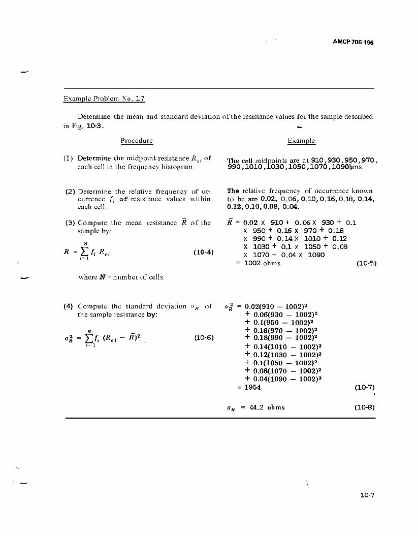
AMCP 706-196


Determine the mean and standard deviation of the resistance values for the sample described in Fig. 10-3. -

Procedure Example

(1) Determine the midpoint resistance Rei of rhe cell midpoints j^ at 910,930,950,970, each cell in the frequency histogram. 990,1010,1030,1050,1070,1090hms.

(2) Determine the relative frequency of occurrence ff of resistance values within each cell.

(3) Compute the mean resistance R of the sample by:

* =ZfiKci (10-4)

ThG relative frequency of occurrence known to be are 0.02, 0.06,0.10,0.16,0.18, 0.14, 0.12, 0.10, 0.08, 0.04.

R = 0.02 X 910 + 0.06 X 930 + 0.1 X 950 + 0.16 X 970 + 0.18 X 990+ 0.14 X 1010+ 0.12 X 1030 + 0.1 X 1050 +0.08 X 1070 + 0.04 X 1090

= 1002 ohms (10-5)

where N = number of cells.

(4) Compute the standard deviation oR of the sample resistance by:

°l = Zfi iRc - Rr i= 1

(10-6)

0.02(910 - 1002)2

+ 0.06(930 - 1002)2

+ 0.1(950 - 1002)2

+ 0.16(970 - 1002)2

+ 0.18(990 - 1002)2

+ 0.14(1010 - 1002)2

+ 0.12(1030 - 1002)2

+ 0.1(1050 - 1002)2 + 0.08(1070 - 1002)2

+ 0.04(1090 - 1002)2

1954

oB = 44.2 ohms

(10-7)

(10-8)

10-7

AMCP 706-196

procedure yields a complete, nonredundant set of circuit equations. The node potentials calculated by solving the circuit equations can be used directly to determine "stress" levels and performance characteristics, such as terminal-to-terminal voltages, current flows, power dissipations, gains, velocities, pressures, forces, and torques.

The first step in analyzing a node potential model is to identify all independent nodes (junctions) where three or more circuit branches meet. Usually, the ground or stationary node is selected as a reference; then the current in each branch is expressed in terms of the node potentials and the branch impedance. Kirchhoffs law (sum of currents into a node is zero) is then applied at each node. The resulting simultaneous equations are set up in matrix form and solved by a computer using a matrix inversion program.

The sound practice cf verifying the mathematical model ought to be followed by comparing the computed results with measurements taken from a breadboard model of the circuit, or from a working model of the mechanical system. It is essential that all parameter values be the same in both the mathematical and physical models. The performance c£ the physical model ought closely to approach the original design performance goals. If these goals are not met, the basic design must be modified.

If the construction cf a mathematical model cf the system is not feasible, a physical model sometimes can be used fix the variability analysis. The physical model is similar to a conventional model, except that it must provide means for conveniently varying parameters.

When a suitable model has been developed, variability data for all component parts are needed so that they can be applied to the model to observe and interpret its response. Three variability analysis techniques are discussed in the paragraphs that follow.

10-5 WORST-CASE METHOD

The worst-case method of variability analysis is a nonstatistical approach (Refs. 1,18) that can be used to determine whether

it is possible, with given parameter tolerance limits, for the system performance characteristics to fall outside specifications (Fig. 10-5). The answer is obtained by using system models in which parameters are set at either their upper or lower tolerance limits. Param- eter values are chosen to cause each performance characteristic to assume first its maximum and then its minimum expected value. If the performsnce characteristic values fall within specifications, the designer can be con- fident that the system has high drift-reliability. If specifications are exceeded, drift type failures are possible, but the probability of their occurrence remains unknown.

Nominal param atar

values

L.

Vary parameters- one »t « time

Mathematical mod«!

P*Hotmific« character I« tic

nominal

Performance characteristic

values

| Performance R characteristic 1 wont cat*

value*

' ■

B value*

e»fttral etefiwfi*« le Fifty li

1 Partial

derivative* 1 . Sign* '

FIGURE 10-5. Worst-case Method'

Worst-case analysis is based on expressing the model performance parameters Vt as functions cf design parameters Px , P2> •••> P„ and expanding these functions in Taylor series about the nominal values. The design parameters include all pertinent part characteristics, inputs, loads, and environmental factors. Tet the model for a performance parameter V, be:

vi=y(P1,p2,P3,...,pn) (lo-io)

The linear expression which relates changes in Vi to changes in the design parameters Pt ,P„ ...,P„ is:

10-8

AMCP 706-196

AV:

where

(10-11)

dVjßPj - partial derivatives of the performance parameter Vj with respect t~ the design parameter Pf

0 = evaluated at the nominal conditions, usually the mean values

£j> = the variation of design parameter Pjmin P. =P- I JO

or Pim„r — P; 0

A set of these equations must be derived to relate all performance factors to all design variables. The partial derivatives of the Vt

with respect to each dependent variable Pj must be computed. Several techniques for calculating these derivatives are given in Refs. 2, 3,4, and 5.

One of the most important steps in a worst-case analysis is to decide whether to use a high or low parameter-tolerance limit for each component part when analyzing a specific performance characteristic. If the slope c£ the function that relates a parameter to a perfonnance characteristic is known, the selection of parameter limit is easy: when the slope of the parameter function is positive, the upper tolerance limit is chosen if the maximum value of the performance characteristic is desired. For parameter functions with negative slopes, the lower tolerance limit corresponds to the maximum perfonnance- characteristic value.

An important part of worst-case analysis is to determine the sensitivity of system performance to variations in input parameters. Although several definitions of sensitivity are found in the literature (Refs. 4 and 6, for example), the sensitivity of a systsn essentially is measured as the effect of parameter variations on the system performance. In equation form, sensitivity can be expressed by:

9 = - **> bp. (10-12)

where

Su = the sensitivity of the performance measure Vt to the variation in the system design parameter Pj

An alternate form is the normalized sensitivity:

'P,o\*Vt a In V,

iViO *pi d In P; MM

(10-13)

which is more frequently used.

The forms of the variation equation which correspond to the two sensitivities are:

AV, = £ Su AP, /-i

AVf

i0

= V J = 1 riQ

(10-14)

(10-15)

Eq. 10-15 is more convenient when the performance equation is a product of terms and the tolerances are expressed in percent.

If a design fails the worst-case analysis, look at the absolute values of the individual terms in Eq. 10-14 or 10-15. The ones which contribute the most ought to be reduced— they are the bottlenecks. It does little good to reduce the small terms because they have so little effect on the total variation. It is not unusual to have well over half the variation due to one or two parameters. If several performance parameters have too much variation, the major contributors ought to be listed for each. If a few parameters are causing most of the difficulty, attention can be devoted to them. If not, an extensive redesign might be necessary.


10-6 MOMENT METHOD

Statistics are combined with circuit- analysis techniques in the moment method to

10-9

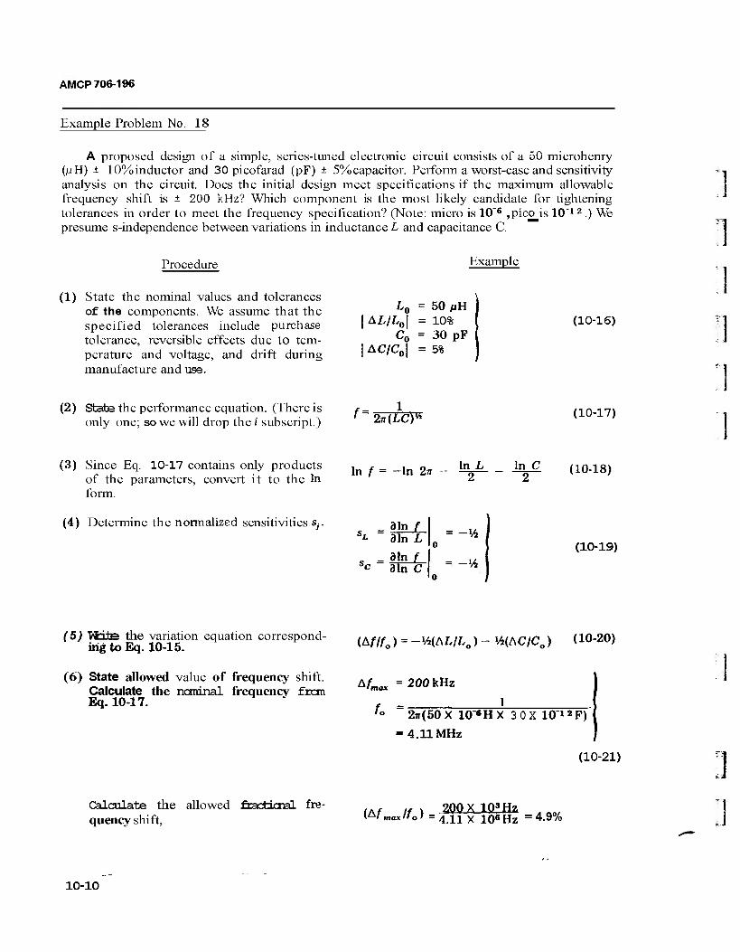
AMCP 706-196


A proposed design of a simple, series-tuned electronic circuit consists of a 50 microhenry (MH) ± 10%inductor and 30 picofarad (pF) ± 5%capacitor. Perform a worst-case and sensitivity analysis on the circuit. Does the initial design meet specifications if the maximum allowable frequency shift is + 200 kHz? Which component is the most likely candidate for tightening tolerances in order to meet the frequency specification? (Note: micro is 10"6 ,pico is 10n 2 .) We presume s-independence between variations in inductance L and capacitance C.

Procedure Example

]

(1) State the nominal values and tolerances of the components. We assume that the specified tolerances include purchase tolerance, reversible effects due to temperature and voltage, and drift during manufacture and use.

L0 = 50 pH \AL/L0\ = 10%

C0 = 30 pF | AC/C0| = 5%

(10-16)

(2) State the performance equation. (There is only one; so we will drop the i subscript.) 2JT(LCP

(10-17)

(3) Since Eq. 10-17 contains only products of the parameters, convert it to the In form.

In f = -In 2n - l^~ ln

nc (10-18)

(4) Determine the normalized sensitivities Sj. 31n f 31n L

_ din f 31n C

(10-19)

(5) TO±te the variation equation corresponding to Eq. 10-15. (Aflfo) = ~ lMAL/L0) - 14(AC/C0) < 10-2<>)

(6) State allowed value of frequency shift. Calculate the nominal frequency frcm Eq. 10-17.

A/m„ =200 kHz

fo = 2n(50X 10"«HX 3 OX 10"*2F)

4.11MHz

(10-21)

Calculate the allowed fractional frequency shift,

(Af if ) 20QX 103Hz W max If o * =4.ii x 10« Hz =4.9%

10-10

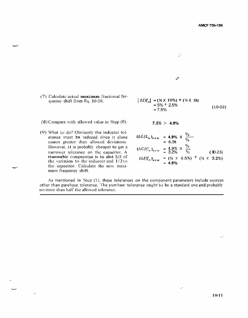
AMCP 706-196

(7) Calculate actual maximum fractional frequency shift from Eq. 10-20. Af/fo\ = (V4 X 10%) + (V4 X 5%)

= 5% + 2.5% = 7.5%

(10-22)

(8) Compare with allowed value in Step (6). 7.5% > 4.9%

(9) What to do? Obviously the inductor tolerance must be reduced since it alone causes greater than allowed deviations. However, it is probably cheaper to get a narrower tolerance on the capacitor. A reasonable compromise is to alot 2/3 of the variation to the inductor and 1/3 to the capacitor. Calculate the new maximum frequency shift.

(AC/C0)ncl

= 4.9% X = 6.5%

= 4.9% = 3.2%

lh

X Zl (10-23)

= (% X 6.5%) + (V5 X 3.2%) = 4.9%

As mentioned in Step (1), these tolerances on the component parameters include sources other than purchase tolerance. The purchase tolerance ought to be a standard one and probably no more than half the allowed tolerance.

10-11

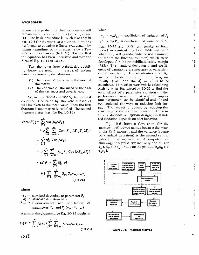
AMCP 706-196

estimate the probability that performance will remain within specified limits (Refs. 1, 7, and 18). The basic procedure is much like that in par. 10-5 for the worst-case method. First, the performance equation is linearized, usually by taking logarithms of both sides or by a Tay- lor's series expansion (Ref. 18). Assume that the equation has been linearized and is in the form of Eq. 10-14 or 10-15.

Two theorems from statistical/probability theory are used. For the sum cf random variables (from any distributions),

(1) The mean of the sum is the sum of the means.

(2) The variance of the mean is the sum cf the variances and covariances.

So, in Eqs. 10-14 and 10-15,the nominal condition (indicated by the zero subscript) will be taken as the mean value. Then the first theorem is automatically satisfied. The second theorem states that (forEq. 10-14)

where

Vax{AVi} = E Var{S0AP.} 7=1

+ 2E E Cov{S|mAPmSl7AP,} 7=1 m=v"+l

= £Sf, Var{AP,.}

+ 2EL SlmS,7Cov{APmAP,} j= 1 m-j+1

= (O2 = E Sl «? /"=1

n n

+ 2 E E SlmSupmJama) }~1 m-/+l

(10-24)

where

Oj = standard deviation of parameter P;- a* = standard deviation of V(

pmi - linear-correlation coefficient of

parameters Pm and Pj (pmj = Pjm )

A similar development for Eq. 10-15results in

(y* )2 = T sl y >+E E su sim pjm yj yn

= coefficient of variation of P7- yj = y,/P,o

y'i = î/îo = coefficient of variation of V(

Eqs. 10-24 and 10-25 are similar in form (exact in content) to Eqs. 9-34 and 9-35 where pjm =0 (s-independence was assumed, it implies no linear-correlation) which were developed for the probabilistic safety margin (PSM). The standard deviation o and coefficient of variation y are measures of variability or of uncertainty. The sensitivities s(/ or Ssj

are found by differentiation; the aj or 7. are usually given; and the o* or 7* is to be calculated. It is often worthwhile calculating each term in Eq. 10-24 or 10-25 to find the total effect of a parameter variation on the performance variation. That way the important parameters can be identified and, if need be, analyzed for ways of reducing their impact. The impact is reduced by reducing the sensitivity or the standard deviation. The sensitivity depends on systan design; the standard deviation depends on part behavior.

Fig. 10-6 shows a flow chart for the moment method—so named because the mean is the first moment and the variance (square of standard deviation) is the second central (about the mean) moment. A computer routine ought to print out not only the ol7 (or jjj), Sit (or su), but also the product ffySl7 (or

T.7sü)-

1

. i

/ = 1 / = 1 m - j* I (10-25) Figure 10-6. Moment Method

10-12

AMCP 706-196

This method for analytically estimating the drift reliability of a system necessitates that five requirements be satisfied:

(1) Specification limits must be supplied for the performance characteristic of all subsystems under consideration. Performance outside these limits constitutes a subsystem failure.

(2) A way must be found to relate performance of a subsystem to the parameters of its components. This need is met by deriving a suitable mathematical model.

(3) The variability of each parameter from one component to another and in the same component with time and environment must be known or be accurately predictable.

(4) A technique (the propagation of variance formula) must be established to combine this information to produce an estimate of overall variability incorporating the simultaneous effect of all sources of variability.

(5) Variability of performance characteristics must be translated into an estimated probability of failure as an aid in predicting reliability.

It is not easy to convert the standard deviation of V, or the allowed limits on Vt to a probability of failure. As explained in par. 9-3.2, especially Eq. 9-38 and Table 9-1, the s-normal distribution may give a too low probability of failure, while the Chebyshev limit may give too high a probability of failure.

A not unreasonable guess for the probability of failure is the geometric mean of the s-normal and Chebyshev probabilities. Since that is a complicated parameter to calculate, the Reasonable-Engineering-guess has been defined as shown in Table 9-1 ;it is easy to calculate and is reasonably near the geometric-mean.

In the process of applying the moment method, very serious consideration must be given to fulfilling requirements 2, 3, and 5 previously mentioned. Requirement lusually is satisfied by establishing performance characteristic limits as the point where the component ceases to produce the desired characteristic, so that the performance of the associated system becomes inadequate. Require- ment 4 is met by means of the propagation of variance formula.

Development of a mathematical model of a component necessarily goes hand in hand with the desired perfonnance characteristics on which certain limits are placed, and with the determination of parameter degradation with time. It is necessary that the mathematical model relate the internal parameters to the performance characteristics. Essenti- ally, the mathematical model is the set of governing equations that describes both quantitatively and qualitatively the physical significance of all parameters in determining the performance characteristics. Development of the mathematical model requires that the component or design be completely analyzed, from which an analysis of each mode of failure can be determined and related to the influencing parameters. Then, the governing equations can be written. The resulting set of equations usually is programmed on an electronic computer, since this greatly simplifies manipulations of the model. These manipulations include the calculation of the sensitivities (viz., partial derivatives of each performance characteristic with respect to each contributing parameter) and the magnitude of the terms in Eq. 10-24 or 10-25. They help to indicate the relative importance of a particular parameter in determining the variation of the performance characteristic.

Once the performance limits have been established, modes of failures determined, and partial derivatives calculated, the causes and mechanisms of timedependent parameter degradation under environmental operating conditions must be quantitatively evaluated. This evaluation can be accomplished by:

(1) Obtaining reliability and failure data from the nEOTfactutsstr and the user

(2) Analyzing data firm real-time simulated environmental operating tests

(3) Extrapolating data from tests run for a short time period

(4) Simulated tests of individual or multiple parameter configurations

(5) Theoretical analysis (6) Combinations of these methods. It is

essential, of course, that theoretical analyses and simulated testing be related to actual operating experience whenever possible.

Data utilized in evaluating the propagation of variance formulainclude:

10-13

AMCP 706-196

(l)Partial derivatives of each component performance characteristic with respect to each contributing parameter

(2) Parameter mean values (3) Parameter variances (4) Linear-correlation coefficients for

interdependent parameters.

Partial Derivatives The partial derivatives, viz., sensitivities, are quite useful since they show the sensitivity of each performance characteristic to variations in each parameter affecting it. It is usually a good idea to calculate both Sy and stJ (plain and normalized sensitivities). It is also worthwhile printing the product S[}Oj = SyOj to show the total variation in Vi due to Pf.

Mean Values The mean values of the performance characteristics obtained from the model are used to evaluate the ability of the model to simulate the behavior of the actual device. The accuracy of simulation can be determined by comparing the mean performance values derived fron the mathematical model with design centers and with corresponding values obtained frcm empirical tests of the component being analyzed.

Conventional wisdom in the USA has it that the tolerance limits are equivalent to ±3o limits. If all tolerances are divided by a number k to find the standard deviation and (tolerance/ft) is substituted for a in Eq. 10-24 and (relative tolerance//?) is substituted for y in Eq. 10-25,then the factor of k2 could be cancelled frcm both sides of revised Eqs. 10-24 and 10-25 and those equations will be true when the o's and 7's are interpreted as tolerances (absolute and relative). When only tolerance limits (not standard deviations) are known, this latter procedure is recommended. When it finally comes time to estimate probabilities from performance variability, a decision on k wiXL have to be made. But at least, then, we will not have forgotten how we chose k, nor what we meant by it.

Performance Characteristic Variances The performance characteristic variances are indices cf the variability of the behavior of the component, and form the basis for evaluating the component design from the point of view of reliability. Standard deviations can be

used in predicting reliability by expressing performance characteristic tolerance limits in terms of multiples of standard, deviations and by estimating the portion ot the total perfonnance characteristic distribution that lies inside these limits (see Table 9-1).

Breakdown of Variance In the event that an excessively high value of r3riance for a performance characteristic indicates a lower- than-desired reliability, it is essential to locate the source(s) of excessive variability. The breakdown of variance facilitates this step, because it tells what portion of the total variance is contributed by each parameter and, thus, immediately spotlights the major con- tributor (s). Since the contribution of each parameter to the whole depends on both its partial derivatives and its variance, the designer quickly can determine whether reliability can be improved by tightening the parameter tolerance limits (i.e., attempting to reduce parameter variance). He can also modify the design to reduce sensitivity (partial derivative) of the performance characteristic to that particular parameter.

Accuracy of the results of the moment method analysis is subject to four obvious limitations:

(1) The mean value and variance are incapable of reflecting by themselves such characteristics of a distribution as skewness and peakedness. Since these characteristics are not a part of the input to the moment-method, they cannot be expected to appear in its output.

(2) The variations in parameter value and variance with time and environmental conditions must be known accurately to produce an accurate reliability estimate.

(3) The function that relates a perfonn- ante characteristic to some parameter of the device is presented in the moment method by its slope (partial derivative), evaluated at the mean point on the curve. If the curve exhibits a high degree of curvature in the region of interest, the inability of the tangent to adequately represent the curve can be a source of error.

(4) The moment method, like any drift- reliability analysis, yields most useful information when it is applied during a time inter-

10-14

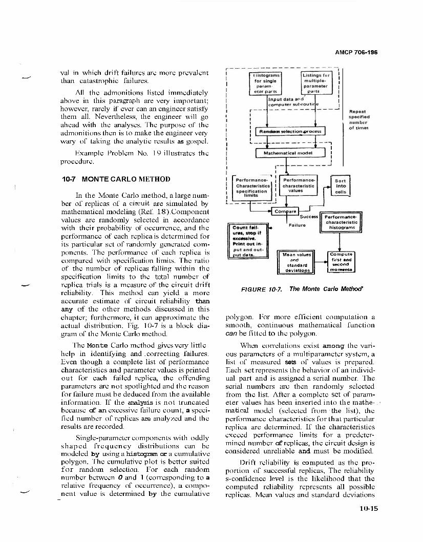
AMCP 706-196

val in which drift failures are more prevalent than catastrophic failures.

All the admonitions listed immediately above in this paragraph are very important; however, rarely if ever can an engineer satisfy them all. Nevertheless, the engineer will go ahead with the analyses. The purpose of the admonitions then is to make the engineer very wary of taking the analytic results as gospel.


10-7 MONTE CARLO METHOD

In the Monte Carlo method, a large number of replicas of a circuit are simulated by mathematical modeling (Ref. 18).Component values are randomly selected in accordance with their probability of occurrence, and the performance of each replica is determined for its particular set of randomly generated components. The performance of each replica is compared with specification limits. The ratio of the number of replicas falling within the specification limits to the total number of replica trials is a measure of the circuit drift reliability. This method can yield a more accurate estimate of circuit reliability than any of the other methods discussed in this chapter; furthermore, it can approximate the actual distribution. Fig. 10-7 is a block diagram of the Monte Carlo method.

The Monte Carlo method gives very little help in identifying and .correcting failures. Even though a complete list of performance characteristics and parameter values is printed out for each failed replica, the offending parameters are not spotlighted and the reason for failure must be deduced from the available information. If the analysis is not truncated because of an excessive failure count, a specified number of replicas are analyzed and the results are recorded.

Single-parameter components with oddly shaped frequency distributions can be modeled by using a histogram or a cumulative polygon. The cumulative plot is better suited for random selection. For each random number between 0 and 1 (corresponding to a relative frequency of occurrence), a component value is determined by the cumulative

Mean values and

standard deviations

Compute first and second

moment«

FIGURE 10-7. The Monte Carlo Method'

polygon. For more efficient computation a smooth, continuous mathematical function can be fitted to the polygon.

When correlations exist among the various parameters of a multiparameter system, a list of measured sets of values is prepared. Each set represents the behavior of an individual part and is assigned a serial number. The serial numbers are then randomly selected from the list. After a complete set of parameter values has been inserted into the mathe- . matical model (selected from the list), the performance characteristics forthat particular replica are determined. If the characteristics exceed performance limits for a predeter- mined number of replicas, the circuit design is considered unreliable and must be modified.

Drift reliability is computed as the pro- portion of successful replicas, The reliability s-confidence level is the likelihood that the computed reliability represents all possible replicas. Mean values and standard deviations

10-15

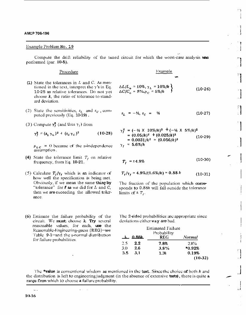
AMCP 706-196


Compute the drift reliability of the tuned circuit for which the worst-case analysis was performed (par. 10-5).

Procedure

(1) State the tolerances in L and C. As mentioned in the text, interpret the y's in Eq. 10-25 as relative tolerances. Do not yet choose k, the ratio of tolerance to standard deviation.

Example

AL/L0 = 10%, yL = 10%/fe \ AC/C0 = 5%,7C = 5%/fe J

(10-26)

(2) State the sensitivities, sL and sc , computed previously (Eq. 10-19) .

(3) Compute tf (and thus y f) from

y2f-(BLyL)

2 + (scycr (10-28)

pLC =0 because of the s-independence assumption.

(4) State the tolerance limit Tf on relative frequency, from Eq. 10-21.

(5) Calculate Tf/yf which is an indicator of how well the specification is being met. Obviously, if we mean the same thing by "tolerance" for f as we did for L and C, then we are exceeding the allowed tolerance.

(6) Estimate the failure probability of the circuit. We irust choose k. Try several reasonable values; for each, lee the Reasonable-Engineering-guess (REG)—see Table 9-1—and the s-normal distribution for failure probabilities.

»t = -'*> sc = -lh (10-27)

yf

yt =

(-'A X 10%/ft)2 +(-% X 5%/fe)2

(0.05/ft)2 +(0.025/ft)2 (10.29)

0.0031/ft2 = (0.056/fe)2

5.6%/fc

Tf =±4.9%

Tflif = 4.9%/(5.6%/fe) = 0.88 k

(10-30)

(10-31)

The fraction of the population which corresponds to 0.88fe will fall outside the tolerance limits of ± Tf.

The 2-sided probabilities are appropriate since deviations either way are bad.

Estimated Failure Probability

k 0 8fifr

2.2

REG Normal

2.5 7.8% 2.8% 3.0 2.6 3.8% *0.92% 3.5 3.1 1.3% 0.19%

(10-32)

The *value is conventional wisdom as mentioned in the text. Since the choice of both k and the distribution is left to engineering judgment (in the absence of extensive tests), there is quite a range fron which to choose a failure probability.

10-16

AMCP 706-196

are computed for each performance characteristic and are quite similar to those obtained by the moment method. A frequency distribution can be computed for each performance characteristic. These distributions can be plotted for further interpretation of the data. Fitting a smooth mathematical function to the distributions often can be helpful in evaluating the tails which tend to be poorly defied unless a large number of replicas have been computed. In no instance, of course, ought the tails of a performance-characteristic distribution extend beyond the worst-case limits.

10-8 METHOD SELECTION

In the early stages of circuit design when realistic tolerances must be selected for the component parts (tolerances that will be economical and yet restrict performance within prescribed limits), the worst-case method is extremely useful. This method makes no attempt to simulate the real system closely, but is intended to give basic design information. If the circuit passes the worst-case test, the variability analysis can be considered complete, since drift failures will not occur if parameter tolerances are not exceeded.

Since it is often not feasible to modify a circuit so it can pass the worst-case test, the probability of successful operation must be estimated. Both the moment and the Monte Carlo methods can be used to make this estimate. The moment method is usually less accurate because of the omission of higher-order terms in the propagation-of- variance formula, but the numerical values of the partial derivatives and breakdown of variance are extremely useful in guiding the modification of the design. The Monte Carlo method is capable of estimating the probability cf success with high accuracy and should be considered when final approval of a design is needed. The moment and worst- case methods are more- suitable during the earlier design stages, since the Monte Carlo method provides little feedback or redesign information. The component-variability data collected with the moment or worst-case method can be expanded later to implement a Monte Carlo analysis.

10-9 COMPUTER PROGRAMS

A number of computer programs for parameter variation analysis are available for use by the engineer. Some of these programs are listed in Table 10-1.

10-9.1 A GENERAL PROGRAM

A FORTRAN listThg of a general program that implements nearly all of the techniques discussed is given in Ref. 8. It is described here briefly. A flow diagram of the program is shown in Fig. 10-8. As can be seen from the figure, the program is keyed to the subroutine which evaluates the performance model. To make the program applicable to any kind of system, no built-in performance model subroutine is included. This subroutine must be supplied by the user of the program (Ref. 4).

The input to the program is a mathematical description of the system model (and the time behavior of the model, if required), the number of random and fixed variables involved, and the means or nominal values of the input variables. Other components of the input are the standard deviations or step sizes in the input variables, the input variable distributions, if available, and the correlations of the input variables. An additional input that is required for some analyses is a selection of values of the element parameters at which the performance model is to be evaluated. Addi- tional programs are described in Refs. 9 through 12.

10-9.2 ECAPAND NASAP

The Electronic Circuit Analysis Program (ECAP) (Ref. 9) is used widely and is available for use on the IBM 1620,7000series and 360 series computers (Ref. 14). It has bean suitably modified for use on a variety of other computers and has some valuable additional features for parameter variation analysis.

The basic versions cf ECAP have the following computational capabilities (Ref. 15):

(1) For DC analysis, ECAP computes partial derivatives cf voltage at a particular circuit node with respect to a circuit parameter in a particular branch; sensitivity of a

10-17

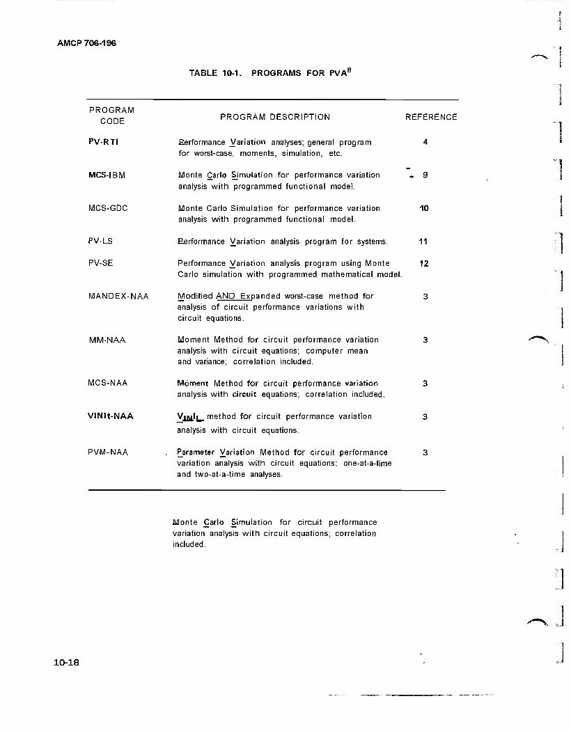
AMCP 706-196

PROGRAM CODE

TABLE 10-1. PROGRAMS FOR PVA8

PROGRAM DESCRIPTION REFERENCE

PV-RTI Eerformance Variation analyses; general program 4 * for worst-case, moments, simulation, etc.

1 MCS-IBM Monte Carlo Simulation for performance variation .9 j analysis with programmed functional model.

'1 MCS-GDC Monte Carlo Simulation for performance variation 10 I

analysis with programmed functional model.

PV-LS Eerformance Variation analysis program for systems. 11 : 1

PV-SE Performance Variation analysis program using Monte 12 Carlo simulation with programmed mathematical model. ?'|

MANDEX-NAA Modified AND Expanded worst-case method for 3 analysis of circuit performance variations with , circuit equations. j

MM-NAA Moment Method for circuit performance variation 3 '"""""N analysis with circuit equations; computer mean and variance; correlation included.

MCS-NAA Moment Method for circuit performance variation 3 analysis with circuit equations; correlation included.

VINIt-NAA VfKfl^ method for circuit performance variation 3

analysis with circuit equations.

PVM-NAA Parameter Variation Method for circuit performance 3 variation analysis with circuit equations; one-at-a-time and two-at-a-time analyses.

Monte Carlo Simulation for circuit performance variation analysis with circuit equations; correlation included.

10-18

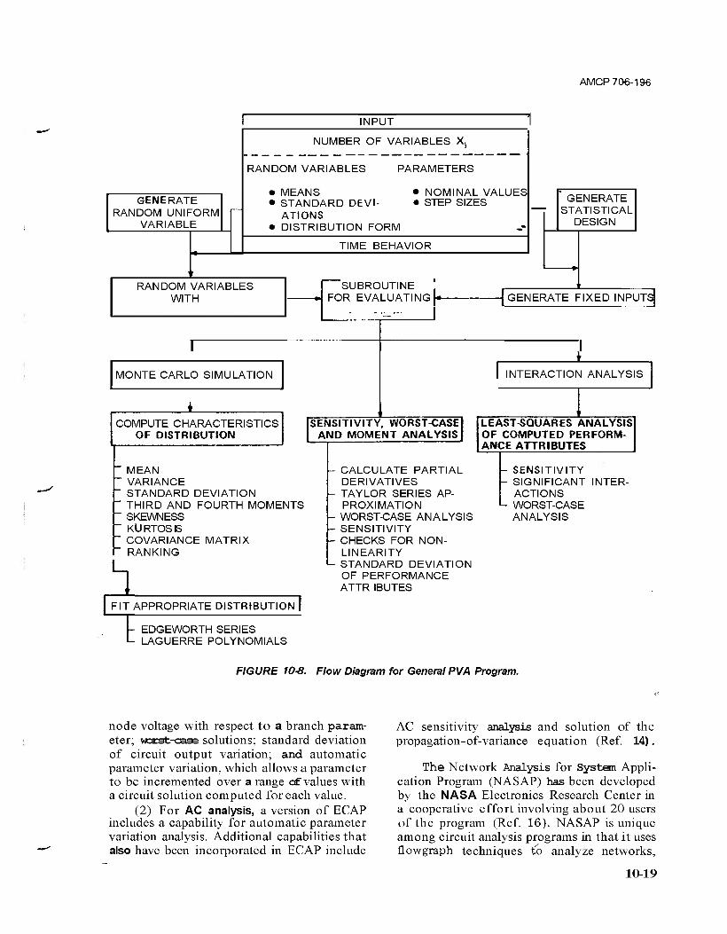
AMCP 706-196

GENERATE RANDOM UNIFORM

VARIABLE

INPUT

NUMBER OF VARIABLES X,

RANDOM VARIABLES PARAMETERS

• MEANS • STANDARD DEVI-

ATIONS • DISTRIBUTION FORM

NOMINAL VALUES STEP SIZES

TIME BEHAVIOR

GENERATE STATISTICAL

DESIGN

RANDOM VARIABLES WITH

SUBROUTINE FOR EVALUATING [•- GENERATE FIXED INPUTS

MONTE CARLO SIMULATION

COMPUTE CHARACTERISTICS OF DISTRIBUTION

_L INTERACTION ANALYSIS

SENSITIVITY, WORST-CASE AND MOMENT ANALYSIS

MEAN VARIANCE STANDARD DEVIATION THIRD AND FOURTH MOMENTS SKEWNESS KURTOSB COVARIANCE MATRIX RANKING

*1

LEAST-SQUARES ANALYSIS OF COMPUTED PERFORM- ANCE ATTRIBUTES

CALCULATE PARTIAL DERIVATIVES TAYLOR SERIES AP- PROXIMATION WORST-CASE ANALYSIS SENSITIVITY CHECKS FOR NON- LINEARITY STANDARD DEVIATION OF PERFORMANCE ATTR IBUTES

- SENSITIVITY - SIGNIFICANT INTER-

ACTIONS L- WORST-CASE

ANALYSIS

FIT APPROPRIATE DISTRIBUTION

I EDGEWORTH SERIES LAGUERRE POLYNOMIALS

FIGURE 10-8. Flow Diagram for General PVA Program.

node voltage with respect to a branch parameter; warst-oase solutions; standard deviation of circuit output variation; and automatic parameter variation, which allows a parameter to be incremented over a range cf values with a circuit solution computed for each value.

(2) For AC analysis, a version of ECAP includes a capability for automatic parameter variation analysis. Additional capabilities that also have been incorporated in ECAP include

AC sensitivity analysis and solution of the propagation-of-variance equation (Ref. 14).

The Network Analysis for System Appli- cation Program (NASAP) has been developed by the NASA Electronics Research Center in a cooperative effort involving about 20 users of the program (Ref. 16). NASAP is unique among circuit analysis programs in that it uses flowgraph techniques to analyze networks,

10-19

AMCP 706-196

instead of matrix-oriented techniques. It also manipulates circuit symbolic parameters instead of actual parameters until the final step of the analysis, This symbol-manipulation feature has some interesting ramifica- tions, one of which is the ability to calculate partial derivatives and sensitivities symboli- cally (Ref, 17).

In addition to the capabilities noted, NASAP incorporates an optimization procedure which eliminates from a circuit input those parameters having less than a pre- assigned amount of influence on circuit performance parameters. The procedure is, in effect, a tolerance analysis (Ref. 17).

NASAP originally was written in FOR- TRAN IV for use on the CDC 3600 computer. It also is now in use on several other computers.

REFERENCES

1. D. G. Mark and L. H. Stember, Jr., "Variability Analysis", Electro-Tech- nology, (July 1965).

2. W. E. Milne, Numerical Calculus, Prince- ton University Press, Princeton, N.J.. 1949.

3. Reliability Analysis of Electronic Cir- cuits, Autonetics Division, North American Aviation, 1964. AD-461 303.

4. A, C. Nelson et al., Development of Reli- ability Methodology for Systems Engi- neering, Vols. I and II, Research Triangle Institute, Research Triangle Bark, North Carolina 27709, April 1966.

5. Abramowitz and Stegun, Eds., Hand- book of Mathematical Functions AMS 55, National Bureau of Standards, U S Government Printing Office (1972).

6. C. Drof, "Computer-Analyze Your Cir- cuit", Electronic Design, (July 21, 1967).

7. R E, Mesloh et äL, Research and Study of Analytical Techniques For Predicting Reliability of Flight-Control Systems, Report FDL-TDL-64-50, Battelle Me- morial Institute, Columbus, Ohio, August 1964.

8. NASA CR-1127 Practical Reliability,

Volume II - Computation, N68-32760, Research Triangle Institute, Research Triangle Park, North Carolina 27709, August 1968.

9. F. P. Kiefer et al., Final Report on Pre- diction of Circuit Drift Malfunction of Satellite Systems, Report ARPA 168-61, IBM, FSD Space Guidance Center, Owego, New York, focJtome Air Devel- opment Center, Griffiss Air Force E&se, 1961.

10. R A. Hay ward and J. I. Ingber, Monte Carlo Flight Performance Reserve Pro- gram, Report GD/C-BTD-65-176, Gen- eral Dynamics, Convair Division, 1966.

11. H. M. Markowitz et al., Launch Vehicle Optimization - Phase II Final Report, Vol. II - Techniques Development, Lear Siegler, hie, 1965.

12. I. Bosinoff et al., Transfer Functions in Mathematical Simulation for Reliability Prediction, Final Report, Report RADC-TDR-63-87, Sylvania Electronic Systems Command, 1963.

13. 1620 Electronic Circuit Analysis Pro- gram, IBM Publication H20-0170-1, IBM Technical Publications Department, White Plains, New York, 1965.

14. H. M. Wall, "ECAP-1966", NEREM Re- cord, 84-5 (1966).

15. H. N. Tyson, G. R Hogsett, and D. A. Nisewanger, "The IBM Electronic Cir- cuit Analysis Program (ECAP)", Pro- ceedings of the 1966 Annual Sympos- ium on Reliability 45-65 (1966).

16. R M. Carpenter, "NASA-Network Anal- ysis for System Application Program ■ Presents Capabilities of a Maintained Program", Computer-Aided Circuit De- sign Seminar Proceedings, Kresge Audi- torium,MIT, 83-94 (1967).

17. R M. Carpenter and W. Happ, "Com- puter-Aided Design - Bart 3, Analyzing Circuits with Symbols", Electronics 92-8 (December 12,1966).

18. NASA CR-1126, Practical Reliability, Vol. I - Parameter Variations Analysis, Research Triangle Institute, Research Triangle Rark, North Carolina 27709, July 1968. (N68-31478).

] 3

10-20-

AMCP 706-196

CHAPTER 11 DESIGN AND PRODUCTION REVIEWS

11-1 INTRODUCTION

Reviews ought to be conducted throughout the life cycle of an item, from concept to field use. The reviews during design and production are perhaps the most important. The preproduction review is essential because drawings and other specifications are never complete, and the design, as it emerges from the design group, rarely is directly suited for mass production. Regardless of the arguments between engineering and production about who is right, the production department's implementation of the drawings and specifications must be reviewed by both the design and reliability groups.

This chapter dwells on the design review to illustrate the kinds of attention to detail that are required. Similar considerations will hold for reviews at the other stages in the life cycle.

The formal review of equipment design concepts and design documentation for both hardware and software is an essential activity in any development program. Standard procedures ought to be established to conduct a review of all drawings, specifications, and other design information by the contractor's technical groups such as equipment engineering, reliability engineering, and manufacturing engineering. This review should be accomplished prior to the release of design information for manufacturing operations. Such a review is an integral part of the design-checking reviews. Responsible members of each reviewing department meet to consider all design documents, resolve any problem areas uncovered, and signify their acceptance of the design documentation by approving the documents for their departments.

Reliability engineering, in conjunction with the equipment engineering groups, ought to conduct an intensive review of the system during initial design. TSie design review includes the following major tasks:

(1) Analysis of environment and specifications

(2) Formal design review of engineering information

(3) Reliability participation in all checking reviews. -

Prior to the formal design review, the requirements defined in applicable military and equipment specifications are reviewed. The expected environmental extremes of the system are studied £e determine suspected detrimental effects on equipment performance. Checklists, based on these studies, are prepared to assure that the objectives of formal design reviews are fulfilled.

The formal design review, which is instituted prior to the release of drawings, is intended to do the following:

(1) Detect any conditions that could degrade equipment reliability.

(2) Provide assurance of equipment conformance to applicable specifications.

(3) Assure the use of preferred or standard parts as far as practical.

(4) Assure the use of preferred cir- cuitry as far as possible.

(5) Evaluate the electrical, mechanical, and thermal aspects of the design.

(6) Provide stress analysis to assure adequate part derating.

(7) Assure accessibility of all parts that are subject to adjustment.

(8) Assure interchangeability of similar subsystems, circuits, modules, and subassemblies.

(9) Assure that adequate attention is given to all human factors aspects of the design.

(lO)Assure that the quality control effort will be effective.

This formal design review is conducted with schematic diagrams, initial parts lists, layout drawings, design and development reports, technical memoranda, and breadboard test results. To insure that the recommendations of the design review group are canied out and are incorporated in all released drawings, reliability engineering personnel should attend all of the förri. checking reviews.

A detailed schedule for design review must be included in program plans developed for a system design effort. This schedule shows the names cf personnel responsible for

11-1

AMCP 706-196

the review. The final program plans must also include copies of typical checklists to be used in the design review program.

All major changes to the system must be subjected to design review. This review will be similar to that performed during initial design. All subcontracted portions of the system are also subjected to a design review. Recommen- dations are to be made to subcontractors for corrective action as required, and to the quality control group for incoming inspections.

11-2 ORGANIZING FOR THE REVIEWS

Design review teams ought to include:

(1) Technically oriented personnel from all groups associated with the product

(2) Design specialists frcm groups that have no direct association with it.

Customer participants also may be present, usually at the critical firaL review. Normally, however, participation ought not to exceed 20 people in order to maintain effective con- ttriL and prevent undue loss of time. Frequent- ly, the experience of the members of the design review team provides the knowledge for a "design break-through" which might not otherwise occur.

The prime task of the design review team is to conduct a detailed design review of the system, including subcontracted items, during the development phase and to XSJöS* all design changes during the preproduction phase. The design review team also viH review the data developed during system tests. The development phase design review is divided into two levels: (1) conceptual review and (2) development review. The conceptual review is conducted after the preliminary design is complete and is oriented to unit and subassembly specifimfckns. The developmental review is conducted prior to release of the design to production and is oriented to cabinet and subassembly design (to validate the actual hardware design for compliance with cabinet and subassembly specifications). In addition, special design reviews are held when significant reliability or performance difficulties are identified during manufacturing or testing- Data submissions, except for engineering drawings, ought to be as follows:

(1) Drawings, schematics, sketches, flow diagrams, or specifications submitted for review as part of a data package are not required to be in their final form but must contain the final information in a'clear complete format,

(2) All linework, symbols, numbers, and letters must be clearly discernible at normal desk top working distance,

(3) Sketch or drawing numbers and revision numbers will be included,

(4) Reports will include title, issue or revision data, and originating individual or activity,

The functions of design review team members are briefly summarized in Table 11-1.

11-2.1 REVIEW BOARD CHAIRMAN

Personality, position, and technical competence are important factors in the selection of a review board chairman. The task requires a high degree of tact, a sound knowledge and understanding of the design requirements, and an unbiased point of view concerning the proposed design. He ought not to be a member of the design staff or of the reliability or other support groups. The configuration management manager is frequently chosen for this Dosition.

The chairman's duties are as follows:

(1) To establish criteria for selecting specific items for review and the type of review to be conducted.

(2) To schedule reviews at the earliest date consistent with the design and development of each item reviewed.

(3) To coordinate and assist the design organization in the preparation of the design data required for the review.

(4) To insure that preliminary copies of agenda, drawings, and related data are sent to the appropriate organizations. This must be done sufficiently in advance of each review to facilitate their prior evaluation and submission of preliminary comments in preparation for each review.

(5) To chair the design review meeting, supervise publication of the minutes, evaluate comments resulting from reviews, and initiate followup action as appropriate,

11-2

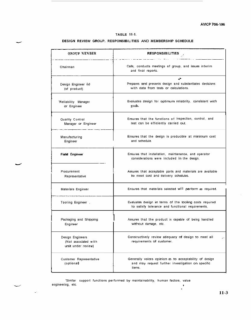
AMCP 706-196

TABLE 11-1.

DESIGN REVIEW GROUP. RESPONSIBILITIES AND MEMBERSHIP SCHEDULE

GROUP MEMBER RESPONSIBILITIES ,

Chairman Calls, conducts meetings of group, and issues interim and final reports.

Design Engineer (s) (of product)

Prepares and presents design and substantiates decisions with data from tests or calculations.

'Reliability Manager or Engineer

Evaluates design for optimum reliability, consistent with goals.

Quality Control Manager or Engineer

Ensures that the functions of inspection, control, and test can be efficiently carried out.

Manufacturing Engineer

Ensures that the design is producible at minimum cost and schedule.

Fielld Engineer Ensures that installation, maintenance, and operator considerations were included in the design.

Procurement

Representative

Assures that acceptable parts and materials are available to meet cost and delivery schedules.

Materials Engineer Ensures that materials selected will perform as required.

Tooling Engineer . Evaluates design in terms of the tooling costs required to satisfy tolerance and functional requirements,

Packaging and Shipping

Engineer

Assures that the product is capable of being handled without damage, etc.

Design Engineers (Not associated with unit under review)

Constructively review adequacy of design to meet all ,, requirements of customer.

Customer Representative (optional)

Generally voices opinion as to acceptability of design and may request further investigation on specific items.

'Similar support functions performed by maintainability, human factors, value engineering, etc. ,

11-3

AMCP 706-196

(6) To revise the system definition documentation when the proceedings of a review warrant it.

11-2.2 DESIGN GROUP

The design group prepares and transmits preliminary copies of agenda, drawings, and related data to appropriate organizations sufficiently in advance of each review to facilitate their prior evaluation, and provides documentation, drawings, and data required for each review. This may include, as appropriate: block diagrams, layouts, sketches, schematics, interface data and drawings, detail drawings, weigh analyses and graphs, appropriate system or item specifications, failure mode and effect analyses, Cause-Consequence charts (fault trees), predictive reliability estimates, reliability block diagrams, critical item lists, and detail study results (e.g., those from stress- strength and parameter variation analyses).

With support from special groups such as reliability, maintainability, human factors, and logistics, the design group plans, conducts, and makes the design review presentation. ALL design reviews must describe system or end item requirements, configuration, how the requirements have been met by the proposed design, installation considerations, systaan or item interfaces with other systems, ground support equipment, etc.

Included in the design review are items such as anticipated development schedules; reliability, maintainability, system safety, human factors, and value engineering factors; producibility considerations including costs, special tools, and facilities requirements; trade studies; test requirements and plans; perform; ance characteristics, including inputs, outputs,^ and tolerances; and electromagnetic interfer- \N

ence.

The design group participates in the preparation of minutes and the evaluation and classification of comments resulting from reviews. They initiate configuration changes if warranted, followup on all comments that require further study, and provide a list of accountability for all design review comments in order to define responsibility for all design improvements.

11-4

11-2.3 OTHER REVIEW TEAM MEMBERS

The formal inputs from specialized review team members are defined by the individuals responsible for the design group presentation. The essential responsibility of the specialists is to critique the design from the standpoint of the design requirements of their specialty and to offer recommendations for improvements. Thus, reliability and other support personnel contribute to a design review by presenting data on compliance with reliability, maintainability, safety, and human factors engineering requirements and standardization. They may propose study projects to develop improvements in their areas of technical responsibility and competence.

The production engineering staff can add measurably to possible design improvements by supplying manufacturing research data and by applying review recommendations to the refinement cE production and procurement planning.

Quality assurance personnel can review technical data and documentation; provide quality assurance data, reports, and analyses; determine constraints, qualification acceptance, and test requirements as they apply to the quality assurance program; and use review recommendations to refine quality and inspection planning techniques.

11-2.4 FOLLOWUP SYSTEM

To achieve maximum results from a design review, a followup system must be established to insure that all corrective actions are performed. All individuals concerned with a design review must recognize their responsiblility for followup.

Design changes that have been recommended and approved must be incorporated info the system design as early as practical. A proven technique is to provide all design changs information to a closed loop corrective action system established for the project. Good recWdkeeping will avert repeated coverage of the same problems and prevent significant loss ofxnsight. Good continuity and followup enable">3ch successive-review to be

J

AMCP 706-196

directed to new areas as the system design proceeds toward production and vise.

11-3 REVIEW CYCLES

The design review cycle, as subsequently described, must be performed for both system hardware and software- Both the Army and its contractors participate in the design review effort. Typical phases are listed in this paragraph.

11-3.1 TECHNICAL EXCHANGE PHASE

The design review cycle is initiated upon receipt of the preliminary design data package by the contractor's design review team from the engineering group. Preliminary data packages contain all the information necessary for the performance of a design review. A minimum list of the infomation necessary for the perfonnance of a design review is given in pars. 11-4 and 11-5. The independent consult- ants representing the various disciplines ought to contact the counterpart design engineer to initiate technical exchange. Subsequent to this, each consultant documents his comments and recommendations. The multidis- cipline comments and recommendations will be integrated by the design team and forwarded to the engineering group. A documented response from engineering completes the technical exchange phase.

11-3.2 INTERNAL DESIGN REVIEWMEET- ING/AGREEMENT PHASE

Formal, contractor, design review meetings ought to be held a minimum of once a month. All items in the documented response fkom engineering must be included in the minutes of these formal, internal, design review meetings. If the engineering response for any item does not agree with the design review team's recommendation, this item is to be discussed at the meeting. The purpose of these meetings is to seek agreement on all such items. Where agreement is not achieved, available information must be documented and presented to management for resolution. Minutes of internal design review meetings record all items covered at the meetings, specific designs reviewed, and decisions made.

11 3.3 ARMY INVOLVEMENT IN INTER- NAL DESIGN REVIEW

At the time of submission to the contractor's design review team, the Army is furnished several copies of the same preliminary data package(s) that are submitted to the contractor's design review team. The Army uses the preliminary data packages for information only- All items covered at the design review meetings are included in the meeting minutes. Army personnel can attend the contractor internal design review meeting as observers but do not participate in the discussions.

11-3.4 DESIGN DATA PACKAGE PHASE

The contractor's engineering group re- vises the preliminary data package according to the results of the design review activity and agreements of the internal design review meeting. The updated preliminary data package is submitted to the design review team for review and approval. This package, when approved by the design review team, is called the design data package. Design data packages are submitted to the Army for review and are placed under internal contractor documentation control.

11-3.5 CHANGE DATA PACKAGE

All changes to design data packages must be documented. A change data package is prepared and submitted for internal contractor design change review. An engineering change review is performed to retain configuration control during preproduction and production. Subsequent to contractor formal approval by its design review team, the change data package is forwarded to the Army.

1 1-3.6 PERFORMANCE SPECIFICATION CHANGES

All performance specification change proposals must be submitted to the Army for approval- Changes to the performance specification must be accomplished by contract modificatioqs.

11-5

AMCP 706-196

11-3.7 GOVERNMENT RESPONSE

Within some reasonable period of time after receipt of each contractor submission (except for preliminary data packages), the Army furnishes the contractor with a detailed critique.

11-3.8 UNSATISFACTORY DESIGN DATA

If any design data submitted by the contractor are considered unsatisfactory, and so documented by the Army critique, the contractor must state his planned action.

11-3.9 ARMY/CONTRACTOR REVIEW MEETING

If requested by the contractor, comments resulting from the Army reviews wH. be discussed in informal meetings between the Army and the contractor. Al items covered at the meeting are included in the meeting minutes.

11-3.10 STANDARD REVIEW

System data items that include technical design standards ought to be reviewed by the contractor's design review team for complete- ness and adequacy as a design standard. Sub- sequent to this review, the detailed system data are submitted to the Army for review and comment.

11-3.11 SUBCONTRACTOR .. VIEW

DESIGN RE-

A design review of subcontracted items must be performed. The contractor design jsnaj unit treats subcontracted items like contractor-prepared items.

11-4 MINIMUM REQUIREMENTS IN CON- CEPTUAL-PHASE REVIEW

The applicable documents listed in system specification and data packages are the basis for the review. Each conceptual review considers the results of the engineering activity documented in the data package. A data

package is prepared after engineering has completed the following activities:

(1) Hardware: (a) Prepared functional block dia-

grams, including interfaces. (b) Partitioned the diagram into

units (cabinets), new and modified. (c) Allocated system reliability re-

quirements to the unit level. "" (d) Prepared a development specifi-

cation for each unit to include reliability, maintainability, and mechanical packaging requirements.

(e) Prepared cabinet block dia-

grams- (f) Partitioned the cabinet into sub-

assemblies. (g) Allocated cabinet requirements

to the subassembly level. (h) Prepared design specifications

for each subsystem and circuit subassembly (including outside vendor items). Include reliability, maintainability , and mechanical packaging requirements.

(2) Software: (a) Identified functions to be imple-

mented within the system computer, identified subroutines required for each function, and estimated memory and computation time required for each subroutine.

(b) Prepared a development specification for each computer subroutine.

(c) Defined major functions of the computer program.

(d) Defined detailed functional requirements.

(e) Defined data requirements with respect to system environment, parameters, and capacities.

The conceptual-phase data-package ought to include at least the following.

(1) Hardware: (a) System description that clearly

relates to the system performance specification while unmistakably giving an overview cf system operation

(b) Equipment development specification for each unit (cabinet) with detailed references to the system performance specification

(c) Functional block diagram that

. J

11-6 -

AMCP 706-196

includes signal flow and characteristics as well as clearly delineating those portions of the system/cabinet involved in each operational mode

(d) System interface tabulation (include input/output wire and cable data as well as signal information and characteristics)

(e) Reliability/maintainability concepts and predictions, including a detailed analysis of the reliability model

(f) Government Furnished Equip- ment (GFE) tabulation

(g) Contractor Furnished Equip- ment (CFE) tabulation

(h) Preliminary installation planning data

(i) Digital logic characteristics completely specified (e.g., frequency response, noise margin, fan in/fan out, impedance, reliability, environmental characteristics, and mechanical configuration)

Ü) Concept for computer-aided analysis of linear and digital circuits and mechanical assemblies and structures

(k) System human factors concepts (1) Clear description (electrical,

mechanical) of unit characteristics and function as part of the total system (including a complete and concise listing of interfacedata such as signal levels, impedances, and waveforms)

(m) Design specifications for each circuit subassembly in the unit

(n) Unit functional block diagram (~) including signal flow and characteristics within the unit and interface data (signal and impedance levels, waveforms, etc.) pertinent to all inputs and outputs to the unit

(o) Unit interfaces (inputs and outputs), including signal flow and signal characteristics (e.g., voltage and current levels, frequencies, impedances, and unusual conditions)

(p) Unit power consumption estimate

(q) (r)

tion design (2) Software:

(a) Computer program development specification

(b) Computer interface definition (c) Timing and sequencing de-

finition

Unit weight estimate Unit maintenance and fault loca-

(d) Description of major functions of each program

(e) Input and output data definition (f) Processing descriptions (g) Environmental data (h) System parameters and program

capacity requirements-

11-5 MINIMUM REQUIREMENTS FOR DEVELOPMENTAL-PHASE REVIEW

The applicable documents listed in the system specification and data packages previously reviewed provide a basis for developmental review. Each such review considers the results of the conceptual design reviews documented in the data package. Such packages are prepared for each unit, circuit subassembly (including outside vendor items), and for the computer programs after engineering has completed the following design activities:

(1) Hardware: (a) Designed a unit (cabinet) to per-

form the desired functions. (b) Performed trade-off and design

analyses. (c) Prepared engineering sketches to

document the cabinet design (including schematics, block diagrams, parts list information, and assembly layouts).

(d) Documented a description of unit operation and recommended method of test.

(e) Designed subsystem and circuits to perform the desired function.

(f) Analyzed and tested the design, utilizing engineering breadboards and computer-aided analysis techniques where applicable.

(g) Prepared engineering schematic and parts list information to document the,. design.

(h) Documented a description of system operation and arecomrrended method of test.

(2) Software: Data packages must be prepared foreach subroutine after engineering has completed the following design activities:

(a) Prepared computer program product specifications.

(b) Specified functional allocations. (c) Prepared s6orage allocations.

11-7

AMCP 706-196

(d) Prepared functional flow diagrams.

(e) Prepared narrative descriptions. (f) Defined modularity. (g) Selected subroutines,

The developmental data package ought to include at least the following.

(1) Hardware: (a) Engineering schematics, block

diagrams, interunit wiring, and parts list information

(b) Nonstandard electrical and mechanical part specification sheets

(c) Description of unit operation supporting compliance with unit specification

(d) Recommended method of calibration, alignment, and test

(e) Reliability prediction for the unit (include electrical and mechanical stress (fata). The prediction ought to include a detailed explanation of the reliability model, including substantiated failure rates and hardware content of each block of the reliability model.

(f) Front panel drawings of cabinets having display and control functions (include human factors data)

(g) Mechanical design layouts and assembly diagrams (include structural and thermal analyses)

(h) Engineering schematic and parts list information

(i) Description cf circuit operation supporting compliance with circuit specifications

(j) Reliability prediction for the subassemblies (include electrical and mech-

anical stress data). The model used as the basis for these predictions will be included.

(k) Information such as signal flow paths, signal levels, impedances, gains, waveforms, bias levels, Boolean * expressions, or truth tables ought to be shown on schematics car otherwise provided.

(1) Maintainability analysis data (m) A variability analysis ought to

be performed. The analysis-will consider the effects of component tolerances, random part selection, aging, and environmental and electrical stresses. The method will be selected from the following: worst-case, moment, or Monte Carlo.

(n) Description of EMI/EMC suppression techniques

(o) Analysis of personnel hazard problems

(p) Test point selection, identification, and tabulations.

(2) Software: (a) Computer program product

specification (b) Computer program and sub-

routine descriptions (c) Subroutine listings.

11-6 CHECKLISTS

Checklists are useful as reminders. A list of items is prepared for the design review team. Each factor is evaluated separately during the design review, and is documented to substantiate the decisions reached, A typical design review checklist is presented in Table 11-2. Appendix A contains a detailed set of checklists that can be used by Army engineers for evaluating a variety of systems,

% i

11-8-

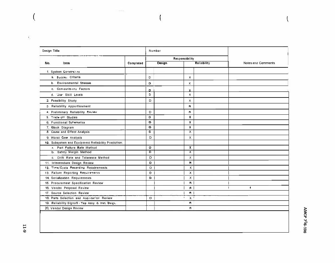
<0

Design Title Number

Notes and Comments No. Item Completed

Responsibility

Design Reliability

1. System Constraint»

a. Success Criteria D X

b. Environmental Stresses 0 X

c. Compatibility Factors D X

d. Use* Skill Levels D X

2. Feasibility Study D X

3, Reliability Apportionment R

4. Preliminary Reliability Review D R

5, Trade-off Studies O X

6. Functional Schematics D X

7, Block Diagram D X

8. Cause and Effect Analysis D X

9. Worst Case Analysis D X

10, Subsystem and Equipment Reliability Prediction:

4. Part Failure Rate Method 0 X

b. Safety Margin Method D X

c. Drift Rate and Tolerance Method D X

11. Intermediate Design Review D R

12, Time/Cycle Recording Requirements D X

13, Failure Reporting Requirements D X

14. Serialization Requirements D X

15. Procurement Specification Review R

16. Vendor Proposal Review R ( 17. Source Selection Review R

18. Parts Selection and Application Review D X

19. Reliability Slgnoff ■ Top Assy. & ln»t. Dwgs. R

20, Vendor Design Review R i o •si o

w 01

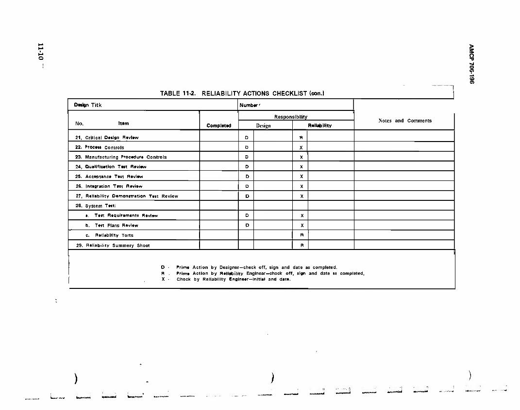
> s o •o

S

to 0)

TABLE 11-2. RELIABILITY ACTIONS CHECKLIST (con.)

Design Titk Number'

No. Item Completed

Responsibility Notes and Comments

Design Reliability

21, Critical Design Review D R

22, Proeeu Controls D X

23. Manufacturing Procedure Controls D X

24, Qualification Tatt Raviaw 0 X

25. Acceptance Tatt Review D X

26. Integration Test Review D X

27, Reliability Demonrtration Tejt Review D X

28. System Tatt:

a, Tart Requirement! Review D X

b. Te«t Plans Review D X

c. Reliability Torts R

29. Reliability Summery Shoot R

0 ■ Prime Action by Designer—check off, sign and date as completed. R . Prime Action by Reliability Enginoar—chock off, sign and date at completed, X ■ Chock by Reliability Engineer—Initial and data.

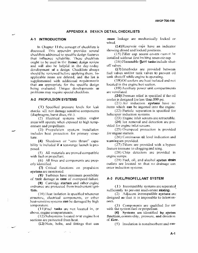
AMCP 706-196

APPENDIX A DESIGN DETAIL CHECKLISTS

A-1 INTRODUCTION

In Chapter lithe concept of checklists is discussed. This appendix provides several checklists addressed to specific design features that influence reliability. These checklists ought to be used in the formal design review and will also be helpful in the day-today development of a design. Checklists always should be reviewed before applying them. In- applicable items are deleted, and the list is supplemented with additional requirements that are appropriate for the specific design being evaluated. Unique developments or problems may require special checklists.

A-2 PROPULSION SYSTEMS

(1) Specified pressure levels for leak checks vüL not damage sensitive components (diaphragms, burst discs, etc.).

(2) Electrical systems within engine areas will operate when exposed to high temperature and propellants.

(3) Propulsion system installation includes heat protection for primary structure.

(4) Shutdown or "zero thrust" capability is included if a test-range launch is proposed.

(5) All materials are proved compatible with fuel or propellant.

(6) All lines and components are properly identified.

(7) Critical functions on propulsion systems are monitored.

(8) Turbines have minimum possibility of tank damage in case of overspeed failure.

(9) Cartridge starters and other engine ordnance are protected from inadvertent ignition.

(10) Heat isolation is specified whenever structure, electrical components, or other heat-sensitive systems can be damaged by high temperature.

(1 l)Fuel tanks are not located in, or above, engine compartments.

(12) Subsystems located near engine hot sections are protected from heat.

(13) Nuts, bolts, and fittings that can

cause leakage are mechanically locked or wired.

(14)Reservoir caps have an indicator showing closed and locked positions.

(15) Filler cap access covers cannot he installed without first locking reservoir cap.

(16) Flammable fluid tanks include shutoff valves.

(17) Interlocks are provided between fuel valves and/or tank valves to prevent oil tank shutoff while engine is operating.

(18) Oil coolers are heat isolated and not located in the engine hot section.

(19) Auxiliary power unit compartments are ventilated.

(20) Pressure relief is specified if the oil cooler is designed for less than 200 psi.

(21) Air induction systems have no items which can be ingested into the engine.

(22) Particle separation is specified for helicopter induction systems.

(23) Engine inlet screens are retractable. (24) Ice removal and detection are pro-

vided for engine inlet screens. (25) Overspeed protection is provided

for engine starters. (26) Continuous oil level indication and

warning are provided. (27) Filters are provided with a bypass

feature immune to clogging and icing. (28) Chip detectors are provided in

engine sumps. (29) Fuel, oil, and alcohol system drain

outlets are located so that no drainage can enter induction systems.

A-3 FUEL/PROPELLANT SYSTEM

(1) Incompatible systems are separated sufficiently to prevent inadvertent nrixtrrj.

(2) Adjacent incompatible systems are designed so that it is impossible to interconnect.

(3) Components are qualified for use with the system fuel or propellant.

(4) Systems are identified by system function, commodity, pressure, and direction of flow.

(5) Insulation is nonabsorbent and can-

A-1

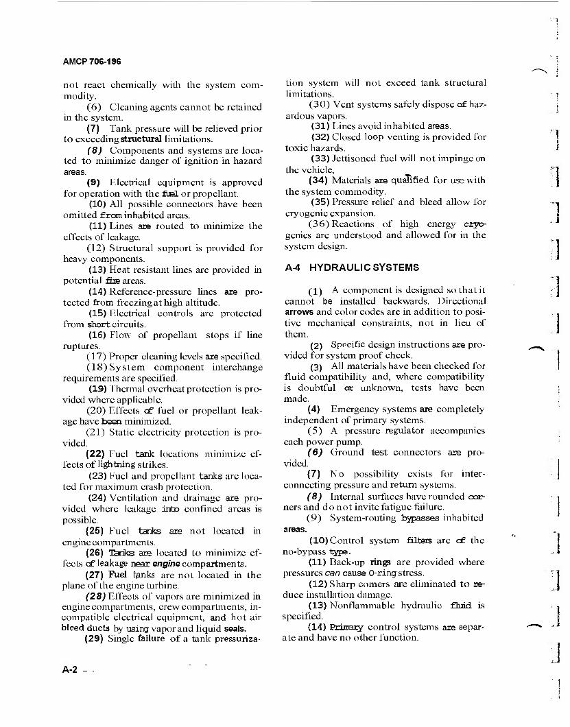
AMCP 706-196

not react chemically with the system commodity.

(6) Cleaning agents cannot be retained in the system.

(7) Tank pressure will be relieved prior to exceeding structural limitations.

(8) Components and systems are located to minimize danger of ignition in hazard areas.

(9) Electrical equipment is approved for operation with the fuel or propellant.

(10) All possible connectors have been omitted from inhabited areas.

(11) Lines are routed to minimize the effects of leakage.

(12) Structural support is provided for heavy components.

(13) Heat resistant lines are provided in potential fire areas.

(14) Reference-pressure lines are protected from freezing at high altitude.

(15) Electrical controls are protected from short circuits.

(16) Flow of propellant stops if line ruptures.

(17) Proper cleaning levels are specified. (18) System component interchange

requirements are specified. (19) Thermal overheat protection is pro-

vided where applicable. (20) Effects of fuel or propellant leak-

age have been minimized. (21) Static electricity protection is pro-

vided. (22) Fuel tank locations minimize ef-

fects of lightning strikes. (23) Fuel and propellant tanks are loca-

ted for maximum crash protection. (24) Ventilation and drainage are pro-

vided where leakage into confined areas is possible.

(25) Fuel tanks are not located in engine compartments.

(26) Tories are located to minimize effects of leakage near engine compartments.

(27) Fuel tanks are not located in the plane of the engine turbine.

(28) Effects of vapors are minimized in engine compartments, crew compartments, incompatible electrical equipment, and hot air bleed ducts by using vapor and liquid seals.

(29) Single failure of a tank pressuriza-

tion system will not exceed tank structural limitations.

(30) Vent systems safely dispose of hazardous vapors.

(31) Lines avoid inhabited areas. (32) Closed loop venting is provided for

toxic hazards. (33) Jettisoned fuel will not impinge on

the vehicle, (34) Materials are qualified for use with

the system commodity. (35) Pressure relief and bleed allow for

cryogenic expansion. (36) Reactions of high energy cryo-

genics are understood and allowed for in the system design.

A-4 HYDRAULIC SYSTEMS

(1) A component is designed so that it cannot be installed backwards. Directional arrows and color codes are in addition to positive mechanical constraints, not in lieu of them.

(2) Specific design instructions are provided for system proof check.

(3) All materials have been checked for fluid compatibility and, where compatibility is doubtful or unknown, tests have been made.

(4) Emergency systems are completely independent of primary systems.

(5) A pressure regulator accompanies each power pump.

(6) Ground test connectors are provided.

(7) No possibility exists for interconnecting pressure and return systems.

(8) Internal surfaces have rounded cor- ners and do not invite fatigue failure.

(9) System-routing bypasses inhabited areas.

(10)Control system filters are cf the no-bypass type.

(11) Back-up rings are provided where pressures can cause 0-ring stress.

(12) Sharp comers are eliminated to reduce installation damage.

(13) Nonflammable hydraulic fluid is specified.

(14) Primary control systems are separate and have no other function.

A-2

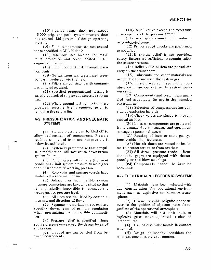
AMCP 706-196

(15) Pressure range does not exceed 15,000 psig, and peak system pressure does not exceed 135 percent of design operating pressure.

(16) Fluid temperatures do not exceed those specified in MIL-H-5440.

(17) Reservoirs are located for maximum protection and never located in the engine compartment.

(18) Fluid does not leak through reservoir vents.

(19) No gas from gas pressurized reservoirs is introduced into the fluid.

(20) Filters are consistent with contamination level required.

(21) Specified preoperational testing is strictly controlled to prevent excessive system wear.

(22) Where ground test connections are provided, pressure line is removed prior to removing the return line.

A-5 PRESSURIZATION AND PNEUMATIC SYSTEMS

(1) Storage pressure can be bled off to allow replacement of components. Pressure readout is provided to insure that pressure is below hazard levels.

(2) System is protected so that a regulator malfunction will not cause downstream system failure.

(3) Relief valves will initially (transient conditions) limit system pressure to no higher than 110 percent of working pressure.

(4) Reservoirs and storage vessels have shutoff valves for maintenance.

(5) Adjacent or incompatible system pressure connectors are keyed or sized so that it is physically impossible to connect the wrong unit or pressure level.

(6) All lines are identified by contents, pressure, and direction of flow.

(7) Separate pressurization sources are specified downstream of primary regulation when pressurizing noncompatible commodi- ties.

(8) Pressure relief is specified where source pressure can exceed the design levels of the system.

(9) Trapped gas can be bled from between components.

(10) Relief valves exceed the maximum flow capacity of the pressure source.

(11) Inert gases cannot be introduced into inhabited areas.

(12) Proper proof checks are performed as specified.

(13) If system relief is not provided, safety factors are sufficient to contain safely the source pressure.

(14) Relief valVe outlets are ported directly to the atmosphere.

(15) Lubricants and other materials are acceptable for use with the system gas.

(16) Pressure reservoir type and temperature rating are correct for the system working range.

(17) Components and systems are qualified and acceptable for use in the intended environment.

(18) Selection of compressions has considered explosion hazards.

(19) Check valves are placed to prevent critical air loss.

(20) Lines or components are protected from damage due to baggage and equipment stowage or personnel access.

(21) Routing of inert or toxic gas systems avoids inhabited areas.

(22) Hot air ducts are routed or insulated to protect structure from overheat.

(23) All direct pressure readout Bour- don tube gages are equipped with shatter- proof glass and blow-out plugs.

(24) Components cannot be installed backwards.

A-6 ELECTRICAL/ELECTRONIC SYSTEMS

(1) Materials have been selected with due consideration for operational environment such as explosive or corrosive atmo- spheres.

(2) It is not possible to ignite or contribute to the ignition of adjacent materials regardless of the operational atmosphere.

(3) Materials will not emit toxic or explosive gases when operated at elevated temperatures.

(4) Use of dissimilar metals in contact is avoided.

(5) Design philosophy considers the most extreme possible environment.

A-3

AMCP 706-196

(6) System operation is not degraded by temperature extremes.

(7) System design provides compensa- tion such as hermetic sealing and pressurization for all pressure-sensitive elements.

(8) Components used in areas with flammable fluids are incapable of causing ignition.

(9) Wiring and component identification are proper.

(10) Routing of wires and location of components will not impose undue mechanical strain on termination points under any combination of anticipated service conditions.

(11) Routing of wires and location of components do not create interference with adjacent systems.

(12) Connections and terminations aus at an absolute practical minimum.

(13) Sensitive circuits are isolated where degradation can be induced by adjacent circuits.

(14) Positive protection is provided for terminal blocks to prevent shorts resulting from contact with miscellaneous debris or from elements of the environment.

(15) Connectors are limited only to those applications requiring frequent discon- nection.

(16) Sufficient space is allowed around connectors for engaging and disengaging, particularly where wrenches are required.

(17) Termination of power and signal leads on adjacent pins of connectors is avoided.

(18) Elements of a redundant system do not pass through the same single connector as elements of the primary system.

(19) Special tools, materials, and processes clearly are specified in the design.

(20) All reasonable effort has been ex- pended to eliminate the possibility of the system contributing to flame propagation or toxic outgassing.

(21) Polyvinyl chloride or other low temperature polymers are not used as wire insulation (high temperatures are always a hazard).

(22) External power receptacles are located as far as possible from points of potential flammable vapor or fluid concentration.

(23) Lead-acid batteries are vented to areas where ignition is not possible.

A-4

(24) Battery vent outlets are designed to eliminate vent system back flow and so that battery acid cannot be ejected from the vent outlet.

(25) Equipment is protected from lightning strikes.

(26) The basic structure has been analyzed to insure compliance with electrical bond- ing requirements, particularly in areas of discontinuity. ~

(27) Electrical shielding is specified wherever it is necessary to suppress radio- frequency interference and other sources of spurious electrical energy.

(28) Circuits and equipments are protected from overload.

(29) It is not possible to induce a dangerous vehicle circuit overload from a malfunction of the ground systan in the power circuits.

(30) It is not possible to induce a dangerous ground system circuit overload from a malfunction of the vehicle power circuits.

(31) Primary and redundant system circuits are not supplied from the same power bus or circuit breaker.

(32) Fuses and circuit breakers are easily accessible and are provided with a visual means to indicate their condition (open or closed).

(33) All elements requiring periodic service are accessible.

(34) Protection is provided from the hazards of loose articles, tools, and debris.

(35) Access covers, components, or equipment requiring specific installation orientation have asymmetric mounting features.

(36) Access is designed for easy handling of heavy components.

(37) Interlocks, shielding, safety guards, barriers, and warning markings have been specified where a personnel hazard can exist.

(38) Handholds, mechanical guides, rails or slides are specified wherever handling of slippery, bulky, heavy, or otherwise hard-to- handle equipment is involved.

(39) Electrical wire bundles avoid routes adjacent to fuel lines, hot air ducts, or mechanical linkages.

(40) High temperature wire and cable insulation is specified for designated fire zones and near high temperature sources.

(41) Routing provides for slack and a

1

J

J

AMCP 706-196

service loop with enough excess wire for three connector replacements.

(42) Wires attached to normally moving parts are routed to twist-with rather than bend-across adjacent moving parts.

(43) Supports are provided to prevent abrasion or chafing of wires and cables.

(44) System-verification test-circuits do not indicate the command; rather, they indicate the actual response of the system.

(45) Power application will not actuate critical circuits as a result of function switches that may be cycled without, indicating the on-off position during a power-off phase (i.e., push-on/push-off switches).

(46) Complex system operational .test requirements are minimized during actual use.

(47) Continuous monitoring is provided for tests requiring judgments rather than standards.

(48) Test points are provided for rapid malfunction isolation.

(49) Connectors and other delicate protrusions cannot be used as footholds or for mechanical leverage.

(50) Maintainability specifications identify any hazards involved in removing, replacing, and testing of elements in the system.

(51) .Ml power can be isolated from specific equipment to allow maintenance or removal.

A-7 VEHICLE CONTROL SYSTEMS

(1) Design is as simple as possible for the task it. will perform.

(2) Electrical and mechanical components are compatible mutually and with the anticipated service environment.

(3) Limiting devices, emergency dis- connects, alternate systems, or other safety measures are incorporated to safeguard critical parameters if a malfunction occurs.

(4) Circuit protection devices do not exist in signal circuit or in other circuits where unsafe control motions of the vehicle would occur if the device opened.

(5) Possibility of electrical cross-connections or phase reversals is minimized.

(6) No component or element of the

system will interfere with crew rescue or escape.

(7) Adequate visual indication of the system operational status is presented to concerned crew members..

(8) Interlocks or limiting devices protect the structure from maneuvers in excess of the structural limit toad factor.

(9) Redundant emergency power systems are provided. ~~

(10) Installation requirements minimize the system vulnerability to defined mission hazards such as enemy action and environmental extremes.

(11) Installation requirements provide the maximum serviceability and maintenance features with a minimum of specialized tools or procedures.

(12) Installation requirements insure that position-sensitive components can be installed only in their proper orientation.

(13) Manual overpower capability is provided with the control system fully en- gaged and operating (piloted aircraft).

(14) Elements of the system are routed, covered, or otherwise protected from jamming frrm dropped or loose items, maintenance operations, cargo shift, etc.

(15) Elements of the system are protected from moisture or fluid accumulation, by- draining potential fluid traps. In addition to normal corrosion hazards, trapped fluids can freeze at high altitudes and jam critical control elements.

(16) Elements of stability, accuracy, and reliability have been evaluated and verified for each component of the guidance and control system.

(17) There is a means of verifying satisfactory operation of each redundant path at any time it is determined that the system or subsystem requires testing.

(18) Redundant paths of the system are located such that an event that damages one path is not likely to damage the other.

(19) Failure in any portion of the system will not cause or create additional or cumulative hazards.

(20) Guards are provided over bolted ends of torque tubes.

A-5

AMCP 706-196

(21) Unsymmetrical components cannot be installed incorrectly.

(22) Consideration h;is been given to pulley diameter versus cable wrap angle and applied force.

(23) Control-column openings are covered by flexible boots.

(24) Control cables are isolated effectively or protected from electrical equipment.

(25) Control mechanisms are located to afford maximum protection to preclude possibility of jamming or damage.

(26) Routing of cables, push-pull rods, and torque tubes considers structural deflection and its effect on function.

(27) Bolt length or reverse bolt installation will not cause system interference.

(28) Sleeves, rub-strips, or guards are provided where contact with stationary objects is possible.

(29) Provisions are made for frequent inspection of fatigue-prone areas.

(30) Inspection plates or access covers will not interfere with movement if installed incorrectly.

(31) Structural deflection will not cause cables to slack sufficiently to cause fouling.

(32) Guards are installed on all vertical pulleys to prevent jamming by foreign objects.

(33) Inspection doors are hinged from the top to prevent falling into any mech- anian.

(34) Bracket attachment structure is reinforced properly to accept applied loads and repeated stresses.

(35) Actuating arms and levers are provided with pins, bolts, or serrations to prevent slippage.

(36) Unfavorable working conditions will not cause maintenance errors.

(37) Turnbuckles and push-pull rods am not subjected to bending forces.

(38) Universal joints are provided where torque tube misalignment can be excessive.

(39) Rod ends have rounded threads. (40) Corrosion-resistant materials are

specified where leaking acid or other corrosive liquids can contact mechanisms.

(41) Insert-bushings are used in attach-

ment fittings in place of removable washers. (42) Bolts are specified to attach rod

ends to hollow tubes. (43) It is impossible to cross-connect in-

advertently any control cable or rod to the wrong fitting.

(44) Pulleys are positively attached to the bearing hub.

(45) Incorrect bolt length-will not cause system interference.

(46) System and its components are compatible in all cases from the standpoint of durability, deflections, wear, and the danger of one component or system creating a hazard by proximity to other components or systems,

(47) Fabrication techniques have not subjected materials to temperatures or stresses which can affect design strength.

A-8 GUIDANCE AND NAVIGATION SYSTEMS

(1) Design will be as simple as possible for the task it will perform.

(2) Electrical and mechanical components are compatible one with the other, and with the anticipated service environment.

(3) Limiting devices, alternate systems, or other safety measures are incorporated when feasible to safeguard critical parameters if a malfunction occurs.

(4) No circuit protection devices exist in signal circuits, or in other circuits that control vehicle motion and where opening cf such a device would produce unsafe motions.

(5) Possibility of electrical cross connections or phase reversals is minimized.

(6) Elements cf stability and accuracy have been evaluated and verified for each component of the guidance and navigation system.

(7) Systan self-check features are provided to allow the operator to detect the presence of systematic random or cumulative error.

(8) A fail-safe or redundant system design philosophy is applied in a manner consistent with mission objectives,

(9) Redundant or double-redundant

3

A-6

AMCP 706-196

design techniques are considered when critical parameters are displayed and arc essential during approach and landing.

(10) There is a means of verifying satisfactory operation of each redundant path at any time the system or subsystem is determined to require testing

(11) Redundant paths of the system are located so that an event that damages one path is not likely to damage the other.

(12) No element of the guidance or navigation system will interfere with crew escape.

(13) Installation requirements minimize the system vulnerability to defined mission hazards such as enemy action or environmental extremes.

(14) Installation requirements provide the maximum serviceability and maintenance features with a minimum of specialized tools or procedures.

(15) installation requirements insure that position-sensitive components can be installed only in their proper orientation.

(16) Adequate visual indication of the system operational status is presented to concerned crew members.

(17) Minimum direct forward visibility is not severely limited by the installation of any navigational system,

A-9 COMMUNICATION SYSTEMS

(1) Redundancy is incorporated where required.

(2) Single component failure will not damage or diminish the use of redundant or related systems.

(3) Redundant systems can be operated from separate and independent power sources.

(4) Adequate design precaution is taken to eliminate or control electromagnetic interference (EMI) effects upon circuit components.

(5) Shielding design complies with MIL-E-6051.

(6) Interference control of the integrated system complies with M1L-STD-826.

(7) System is compatible and in compliance with "worst case" system requirements.

(8) System separation of the transmit-

ter and receiver is such that direct excitation of the receiving antenna cannot exceed 10/.<V.

(9) Status displays are incorporated in all system functions that monitor hazardous operations.

(10) Compatibility with all relay links is possible within the allocated frequency of the proposed communication system desiVn

(ll)Maximum continuous RF exposure of operational personnel or vehicle crew members does not exceed lOmWcm"2.

A-10 PROTECTION SYSTEMS

(1) Explosive vapor detectors are specified where explosive vapors can collect.

(2) Explosive vapor detection system will trigger an alarm at 20 percent of the lower explosive level.

(3) Toxic vapor detectors are specified wherever toxic gases or vapors can enter inhabited areas.

(4) Fire detection systems are specified for all potential fire zones.

(5) Smoke detectors are specified in nonventilated baggage or cargo areas.

(6) Ail possible design action has been taken to prevent false indication.

(7) Hazard warning systems can be re- set to indicate a hazard recurrence.

(8) Explosive vapor detectors can operate in an explosive atmosphere without initiating an explosion.

(9) Deviation from normal perfonnance will cause an explosive vapor detection system malfunction indication.

(10) All detection systems are completely compatible with the environment in which they must operate.

(11) All hazard detection systems receive power from the essential-equipment bus-

(12) Detector reaction time is at its absolute minimum.

(13) Provisions are made to allow periodic system calibration and checking.

(14) Malfunction detection systems sense critical system deviations.

(15) Critical instruments have positive failure warning,

(16) Instrument malfunction flags are not used to designate emergency conditions-

(17) All emergency conditions or malfunctions initiate a warning.

A-7

AMCP 706-196

(18) Emergency conditions requiring immediate action initiate an audible warning in addition to visual warning.

(19) Audible warning is not specified in the communication system when constant monitoring is not required.

(20) Sound levels will not interfere with essential communications.

(21) Verbal audible warnings are clear, concise, intelligible, and reflect calmness and urgency.

(22) Audible warning ovemde is provided where prolonged warning will interfere with effective corrective action,

(23) Volume controls do not reduce warnings to an inaudible level.

(24) Component interlocks are specified whenever out-of-sequence operation can create a system hazard.

A-11 FIRE EXTINGUISHING PRESSIONSYSTEM

AND SUP-

(1) Potential fire zones are identified. (2) Potential fire zones are isolated by

fire barriers or firewalls. (3) Titanium is not used structurally

where it may contact molten metal. (4) Firewalls are as liquid- and vapor-

proof as possible. (5) Access doors have not been in-

stalled in firewalls. (6) Firewalls are not stressed by

mounted equipment. (7) Materials used on the protected

side of firewalls. will not bum as a result of high temperature in the fire zone.

(8) Air ducts passing through fire zones are fabricated to insure fire contain- ment.

(9) Air ducts originating in fire zones can be closed to stop airflow.

(10) Flammable fluid lines with flow into or through a fire zone are provided with shutoff valves.

(11) Fire will have no effect on the operation of shutoff valves or control circuits.

(12) Flammable fluid lines in fire zones are made of stainless steel or equivalent.

(13) Flammable fluid flexible hose will

withstand 2000" F when routed in or near fire zones.

(14) Fire detection is specified for all potential fire zones.

(15) Fire extinguishing systems are specified for all potential fire zones. (Ref. MIL- E-5352.)

(16) The most effective extinguishing agent is specified consistentjvith both safety and design goals.

(17) Toxicity is considered where it is possible for fumes to enter inhabited areas.

(18) Extinguishing agent containers are designed for maximum possible protection from crashloads or gunfire.

(19) Extinguishing agent containers have safety relief.

(20) Visual indication is provided that safety relief has occurred.

(21) Pressure gages are readily accessible for inspection and maintenance.

(22) Squib actuated discharge valves are designed so that electrical connection cannot be made unless the squib is installed.

(23) Interfaces between control systems and other systems cannot cause extinguishing system failure.

(24) Redundancy is specified where in- lays are used in the control system.

(25) Separate initiation circuits and dual squibs are provided for each container.

(26) Routing of control wiring does not pass through potential fire zones unless it can withstand at least 2000°F without system degradation.

(27)Automatic explosion-suppressing devices are considered wherever an explosion can occur too swiftly for crew reaction.

(28) Suppressing-system status is provided to indicate system has actuated.

(29) Flame-proof containers or compartments are specified for storage of items with low ignition temperature or high flame- propagation rates.

(30) Toxic products of combustion are considered when cabin interior materials are selected.

(31) Tests have been specified to determine if combustion products are toxic when unknown or doubtful.

A-8 j

AMCP 706-196

(32) Electrical equipment will not provide an ignition source when operating in any hazardous atmosphere.

(33) Flammable fluid line routing avoids inhabited areas or is restricted.

(34) Complete fire hazard analysis has been made.

(35) Fuel lines and tank structures are designed to contain fuel as much as possible within the system under crash-induced load- ings.

(36) Fuel lines and tanks are protected from penetration during a crash by mounting behind heavy structure and avoiding areas where penetration is likely.

(37) Provisions are made to deactivate systems that can provide an ignition source on crash impact.

(38) Spark-producing metals are not exposed to crash friction.

(39) Flammable fluid components are located where ground contact cannot occur and where crash damage is unlikely.

(40) All possible consideration is given to use of gelled or other ignition-inhibited fuels.

(41) Interior finishes and materials are selected for inability to support combustion and minimum toxic products of combustion.

(42) Flammable materials specified for use in an interior are at a minimum and flame retardants are specified for any flammable material used.

(43) Passenger compartments are provided with fire resistant storage compartments for combustible materials.

(44) Hand fire-extinguishers are provided.

(45) Cargo areas have fire detectingand extinguishing systems.

(46) Ventilation and cargo areas can be closed off during the extinguishing cycle.

(47) Lighting in cargo areas is protected f romdamage and contact with flammables.

(48) System actuation cannot be mis- directed to the wrong fire zone.

(49) A single control handle will shut off flow of flammables and ignition sources.

(50) Audible alarm is provided where fire warning lights may go unnoticed.

(51) Audible alarm override is provided. (52) System actuating switches are pro-

tected from inadvertent operation.

A-12 CREW STATION SYSTEMS

(1) Dimensional allowances for safe crew accommodations and work places comply with the 5th'through 95th percentile.

(2) Surface colors properly depict the appropriate physical hazards by coding.

(3) Shape and location of emergency controls are such that crew members are able to operate them without visual reference.

(4) Operating controls are designed and located to minimize inadvertent activation.

(5) Emergency controls are readily visible and accessible.

(6) Materials and finishes selected for the crew stations are compatible with the environment.

(7) Types and characteristics of auditory and warning devices are suitable for providing the discrimination necessary under all operating conditions. Caution and advisory lights are located outside the flight instrument group. The brightness of the translucent areas of light indicators is at least 150 f t-lamberts in the bright mode.

(8) Displays are designed to minimize reading errors.

(9) Master caution and all warning lights can be dimmed to approximately 15 ft-lamberts when instrument lights are on and all other lights dimmed to approximately 1.5 ft-lamberts.

(10) Labels or placards are plainly legi- ble under both day and night conditions. Warning and caution indicator lights are readily visible to crew members while at their stations.

(ll)Proper equipment is provided to maintain safe cabin temperature and airflow requirements.

(12) Fuel and dl are prevented from contaminating the air in the crew compartments.

(13) Suitable decontamination and fil- tration devices are provided.

(14) Lhere is proper access for the removal and replacement of filters or filter media.

(15) High-pressure, high-temperature bleed air ducts are located to prevent overheating of walls and compartments and the bypass areas containing combustible fluids.

Ä-9

AMCP 706-196

(16) Check valves, shutoff valves, and other devices are provided for sealing off or regulating pressurized compartments.

(17) Insulation of the ducts is located properly and made of materials to prevent heat loss and contact with, or absorption of, combustible fluids.

(18) Range of temperatures in the crew compartment complies with the thermal com- fort zone and specified exposure times for heat and cold.

(19) There are emergency provisions for assisted or unassisted escape from the crew compartment.

(20) Crew personnel are provided with an unimpeded path out of, and away from, the vehicle.

(21) Emergency lighting is incorporated in the crew compartment.

(22) Safety belts, harnesses, and straps are provided.

(23) Crew and their personal equipment are protected from thermal radiation caused by the explosion of nuclear weapons, including eye protection against flashblindness.

(24) Alarms and warning signs are designed, installed, and located so that they can be heard or read directly by crew members.

(25) Fire and overheat systems are designed and located to alert crew members of such conditions.

(26) Portable fire extinguishers are designed and mounted in locations where they are readily usable by crew members.

(27) Circuit overload protection devices are adequate.

(2 8) Interconnecting wires and cables are secured and protected to avoid inadvertent contact or. wire chafing,

(29) Equipment cooling ducts and the equipment are located to provide adequate cooling of hot spots.

(30) Equipment is sufficiently accessible for manual fire extinguisher utilization.

(31) If a bipropellant is used, the oxi- dizer and fuel components are separated as far as possible.

(32) There are propellant shutoff and fueljettison valves.

(33) Electrical wires, cables, and heatproducing equipment are isolated from the propellant components.

(34) All electrically operated motors, valves, solenoids, relays, etc., are of approved explosion-proof type.

(35) All materials used within the pressurized compartments are fire resistant. Inter- ior materials do not generate toxic and noxious gases when exposed to heat and flame.

(36) Electrical and heatproducing items are separated from oxygen systems.

(37) A complete fire detection and extinguishing system is built into the vehicle.

(38) Fire extinguishing agents are compatible with the vehicle structure and environmental control systems.

(3 9) Environmental control system is equipped with filters for noxious gas and noxious gas neutralizing systems.

(40) If a toxic propellant is used, the lines and connections associated with it are routed outside the crew compartment.

(41) Pressurized compartment is sealed off from components that could generate toxic gas.

(42) Pressurized compartments are capable of being vented and purged to remove toxic gas.

(43) A complete toxic gas warning systsiL is installed in the vehicle.

(44) Interior is free from sharp objects that could cause crew injury.

(45) All protrusions are removed, pad- ded, labeled, or otherwise shielded.

(46) All electrical systems are labeled, interlocked, isolated, or otherwise designed to minimize electrical shock.

(47) Adequate provisions for the storage, protection, and accessibility of equipment and supplies are provided.

(48) Electrical power supply is redundant.

(49) An alternate power source is available for environmental control system operations. If not, insure that a stand-by or emergency environmental control system is available.

(50) Emergency power is supplied from a separate source and from an independent power bus.

(51) Vehicle pressure \«ül is designed so that proper quality control and testing procedures will ascertain pressure reliability.

A-20

AMCP 706-196

(52) Crack propagation is limited. (53) Faulty seals can be detected. (54) Where wear or damage can occur,

double seals are used. (55) Seals or sealing devices are designed

so that replacement or emergency repairs can be made.

(56) Shielding is provided adjacent to equipment that could structurally fail and puncture the cabin wall.

(57) Delicate components are located where they will not be damaged while the unit is being worked on.

(58) Internal controls, such as switches and adjustment screws, are not located close to dangerous voltages.

(59) Components that retain heat or electrical potential after the equipment is turned off are not located where maintenance personnel may touch them inadvertently upon opening the equipment.

(60) Irregular protrusions such as cables, wave guides, and hoses are easily removable to prevent damage during maintenance.

(61) Rests or stands are provided on which units can be set to prevent damage to delicate parts. Rests or stands are designed as a part of the basic chassis.

(62) Fold-out construction is provided for units wherever feasible, and parts and wiring are arranged so that they are not damaged when the assembly is opened or closed.

(63) Covers and cases are sufficiently larger than the units they enclose to preclude damage to wires and other components when the cases are removed or replaced.

(64) Comers and edges of covers and cases are rounded for safety while handling.

(65) Ventilation holes in covers are small enough to preclude inadvertent inser- tion of any object that might touch high- voltage sources or moving parts.

(66) Handles are shaped so that they do not cut into the hand of the holder.

(67) Guards or other protection are provided for easily damaged conductors such as high-frequency cables or insulated high- voltage cables.

(68) Plugs with a self-locking safety catch are used in preference to plugs that must be safety-wired.

(69) Internal fillets that might injure the

hands or arms of maintenance personnel are provided with rubber, fiber, or plastic shielding on the edges.

(70) On accesses,that lead to equipment with high voltages, safety interlocks are provided that deenergize the circuit when the access panel is opened. If maintenance is required on equipment with circuits ener- gized, insure that a theater" switch is provided that bypasses the interlock and that automatically resets when the access panel is closed.

(71) Warning labels are provided on all access panels leading to high voltage or moving parts.

A 13 ORDNANCE AND EXPLOSIVE SYSTEMS

(1) Sensitivity, shattering effect, and power of the explosive are evaluated fully for each application.

(2) Degree of sensitivity of the initi- ator is evaluated fully for each application.

(3 ) Materials are without dangerous de- fects, and will resist changes due to aging.

(4) Degree of confinement of the device is evaluated fully for each application. Explosive energy release is more hazardous in areas of closer confinement.

(5) Items with critical manufacturing tolerances are avoided where possible since such items are more susceptible to accidental ignition.

(6) Termination interruptions in the firing circuit are held to the absolute minimum.

(7) Maximum protection from inadvertent operation is provided by proper circuit design and use of safe/arm devices.

(8) The most electrically or mechanically insensitive device commensurate with the application is used.

(9) Specifications for storage comply with existing regulations and requirements.

(10) Specifications for storage do not permit the use of static electricity genera- tors—such as plastic sheets, wraps, and covers—in any part c£ the packing and storage process.

(ll)Test and evaluation are carried out properly through detailed test specifications

A-11

AMCP 706-196

showing test objectives, methods, equipment, personnel, and special precautions necessary as determined by the design.

(12) The insulation for ordnance firing circuits possesses the optimum dielectric characteristics for the design environment.

(13) Shielding to protect the squib and firing circuits from stray voltage is evaluated properly and optimized for each design.

(14) Ordnance circuits are routed with minimum exposure to physical damage and potential electrical ignition sources.

(15) Ordnance control circuit design is compatible with the vehicle shock and vibration environment.

(16) Ordnance devices and the firing circuits have been reviewed separately and as an integrated system, giving strong emphasis to subsystem interfaces.

(17) Applicable range safety manuals have been reviewed for ordnance system performance requirements prior to design selection.

(18) A hazard analysis is conducted on all ordnance systems to evaluate their hazard potential. A hazard analysis is conducted on all liquid-propellant and solid-propellant systems to an acceptable hazard level of operation.

(19) Hazard analysis has identified all potential modes of vehicle failure and has indicated design approaches, corrections, or

recommendations to minimize the level of the indicated hazard.

(20) Design has been corrected in accordance with the findings of the hazard analysis consistent with program objectives.

(21) All hazards have been evaluated either by experiment or empirical knowledge.

(22) Effectiveness and necessity of an explosion suppression and inerting system have been evaluated.

(23) All ignition sources are identified and corrective measures are taken to reduce the probability of their contribution as an explosion source.

(24) Design requirements subject a minimum of personnel to the acceptable hazard level determined by the system hazard analysis.

(25) Fuze/aafing-arming mechanism has at least two independent safing features, any one of which can prevent an unintended detonation. Each is activated by a different environmental input. At least one feature includes an arming delay adequate to spare the user from injury in case of premature functioning of the system. The item is fail- safe when all safing features are subverted.

(26) Detonation of any primer or deton- ator in a fuze/safing-arming mechanism that is in the safe condition will be physically barred from causing further functioning of the explosive train.

A-12

AMCP 706-196

APPENDIX B RELIABILITY DATA SOURCES

B 1 INTRODUCTION

In recent years, a targe number of reliability information centers and data banks have been established. These data banks provide information in a variety of formats useful to reliability engineers. Advances in the field of computer storage and retrieval, microfilming, microfiche techniques, and other processes have made it possible to store and retrieve large quantities of information. Information retrieval techniques have been developed which permit the engineer to retrieve stored data and perform statistical evaluations.

The accumulation of numerical reliability data has been aided technically and economically by the use of computers. Most of the early data banks were established to provide the designer with the information he needed for a specific system development. The more recent programs are broader in scope and have made some efforts to alleviate some of the shortcomings of their prede- cessors. Some early programs have been combined with others or eliminated.

Ref. 4 is a comprehensive listing of Reli- ability and Maintainability sources associated with the Air Force. Three major data banks are described in pars. B-2, B-3, and B-4. Some of the special circumstances that the designer must consider in using data bank information are .discussed in par. B-5. A partial listing of data banks is presented in par. B-6.

B-2 GIDEP, GOVERNMENT-INDUSTRY DATA EXCHANGE PROGRAM

B-2.1 INTRODUCTION

The Government-Industry Data Ex- change Program (GIDEP) was originated in 1959 by the Army, Navy, and Air Force Ballistic Missile Agencies. Known at that time as IDEP—Interservice Data Exchange Program—its intent was to eliminate duplicate testing of parts and components by dis- seminating pertinent test data among Depart- ment of Defense contractors and various

Government agencies, The Navy FARADA program also has "been integrated into GIDEP.

In 1966, both the National Aeronautics and Space Administration and the Canadian' Military Electronics Standards Agency (CAMESA) recognized the value of the data provided by the program and became participants. Today, GIDEP provides the interchange of reliability data to all the military services, participating Government contractors, and numerous Government agencies such as the Energy Research and Develop- ment Administration, Federal Aviation Ad- ministration, Defense Supply Agency, and the Small Business Administration.

GIDEP operates under a charter agreed upon by the Army and Navy Materiel Com- mands, the Air Force Systems and Logistics Commands, and NASA. The Program Man- ager, organizationally located within the Department of the Navy, is responsible for policies and procedures, both national and international. The GIDEP Administration Office located at FMSAEG, Corona, Califor- nia, is the operational ann of the program. Working directly under, and responsible to, the Program Manager, the Administration Office maintains the GIDEP data banks and is responsible for all operational phases of the program. The GLDEP management team includes Government and Industry advisory groups.

Availability of a microfilm reader-printer is the only equipment requirement for the frequent GIDEP data user. Participants are not subject to fees or assessments of any kind, nor is there any payment for contributions of data. Participation at contractor facilities usually is considered part of the normal reliability or quality assurance program. However, with the recent issuance of Regulations by the Military Services and NASA, participation is now becoming a mandatory requirement.

The objectives of the GIDEP program are to:

B-l

AMCP 706-196

1. Reduce or eliminate duplicate ex- penditures for development parts and components

2. Increase the confidence level in the reliability of systems using these parts and components

3. Expedite research and development projects by avoiding repetition of tests previously accomplished

4. Assist in the preparation of more realistic proposals

5. Standardize procedures for reporting test information

6. Encourage direct intercontractor communications among technical personnel working on related projects

7. Generate information for an alternate source of parts through more depend- able data

8. Create a general source for test data 9. Provide for the exchange of test

equipment calibration procedures and related metrology data.

This description has been adapted from Ref. 3.

B-2.2 FUNCTIONS

GIDEP data are contained in four separate information banks: the Engineering Data Bank, the Failure Experience Data Bank, the Failure Rate Data Bank, and the Metrology Data Bank. No classified or company proprietary information is included.

B-2.2.1 Engineering Data Bank

The Engineering Data Bank contains primarily., laboratory data relating to parts, components, and materials. These data cover Qualification and Environmental Testing, Re- search and Development, Evaluation Re- ports, and other meaningful engineering data such as nonstandard part justification, test planning, and manufacturing processes.

B-2.2.2 Failure Experience Data Bank

The Failure Experience Data Bank contains failure experience data; failure analysis reports from the field, laboratory, and production; and information from a pilot effort

for a Defective Parts and Components Con- trol Program (DPCCP), which includes failure analysis data by component types derived from an operation and maintenance level. The function of the DPCCP is to identify and eliminate or cor»trol defective parts, Methodology includes both the avoid- ance of specifying suspect parts in new designs and the purging of these suspect parts from current Government inventory if required. "™

Part of the Failure Experience Data Bank is an important function known as the ALERT system. The ALERT is a highly effective means of rapidly providing all participants with information concerning an actual or potential problem involving a part, material, test equipment, process, or safety hazard. Any participant who finds a situation that he feels to be of general concern to other participants, fills out an ALERT form. The ALERT form is submitted to the Administration Office where it is reviewed and distributed to all participants as an ALERT. Generally, this process is completed within 24 hr. The ALERT system may be used for any type of pertinent information relating to any of the data banks. It is issued to identify such items as faulty design, faulty test equipment or calibration procedures, or other production and processing problems.

B-2.2.3 Failure Rate Data Bank (FARADA)

The Failure Rate Data Bank contains field performance data relating to parts and components. Detailed information concerning failure rates, stress levels, mean time to repair, level of test specification, failure mode, test environment, and other pertinent information is contained in the Failure Rate Data Bank. The FARADA program—which collected field experience and reliability demonstration test data for use in Reliability Prediction, Spares Provisioning and Logistics Support studies- has been integrated into GIDEP as of July 1973. This has enlarged the GIDEP data bank and provides a broader range of participating organizations. It also provides parts and components performance data obtained under

1

B-2 ,3

AMCP 706-196

actual field operational conditions, so that correlation studies can be made to compare laboratory tests with field experience.

B-2.2.4 Metrology Data Bank

The Metrology Data Bank contains Cali- bration procedures and general infomation on test equipment. Calibration procedures prepared by both the military and industry, covering most electrical and mechanical test equipment, are available to participants. Under a program called SETE (Secretariat for Electronic Test Equipment), which is aligned with GIDEP, other types of information such as test equipment evaluation reports are available. These reports greatly influence reliability improvement in test equipments and instrumentation. Groups concerned with the measurement of physical and electrical attributes, or development of measurement standards and instrumentation, are primary users of this data bank.

The International Reliability Data Ex- change with the EXACT program is head- quartered in Sweden. Functioning at an international level. EXACT provides for the exchange of reliability test data with a dozen foreign countries. GIDEP provides test reports to EXACT which document successful qualification and evaluation laboratory tests on parts and materials. The increasing use of foreign-made parts in our military systems makes availability of information on those materials of obvious value. EXACT provides for data exchange among all member countries.

B-2.3 OPERATJONS

The GIDEP program operates as a self- regenerating, closed-loop system. Engineer- ing, Failure Experience, Failure Rate, and Metrology data are submitted by Government or industry participants to the Administration Office for inclusion into the GIDEP Data Banks. When a GIDEP Representative submits data to the Administration Office, he assigns it a 9-digit generic index code. The first 3 digits of the code define the major part classification, such as: transformer or antenna. The last 3 pairs of digits provide relative levels

of detail information covering such areas as function, application, construction, and even detailed data such as pressure range, working voltage, power rating, and frequency range- The codes for indexing GIDEP data are contained in the GIDEP Policies and Procedures Manual (Ref. 1).

Once data have been screened and indexed, the index -k placed in the GIDEP computer, and the full report is placed in microfilm cartridges that are distributed along with a hard copy index biweekly to all participants. The Administration Office distributes a complete updated index to all participants annually. Participants may request a computer index search and copies of reports directly from the Administration Office, or they, through a terminal, address any of the four GIDEP data banks individually or collectively. The user can enter a year date to restrict his data search to relatively current information, or he can run an entire historical search of all data in a particular area.

The GIDEP computer is programmed so a participant can initiate a search using any of several approaches. The computer can be addressed to search by GIDEP generic code, manufacturer's part number, key work, industry standard part number, environmental code, or any other fields contained in the data banks. Once information is located, the computer provides the participant with a microfilm reel and access number in addition to a report number. All participants are provided with microfilm indexes. Thus, if a participant does not maintain microfilm records, he can request copies of specific reports or the loan of a microfilm reel frcm the Administration Office.

If an index and computer search fails \o identify participant-required data in the GIDEP Data Banks, the user can initiate an Urgent Data Request (UDR). One of the most powerful tools of the GIDEP program, the Urgent Data Request is a means by which a participant submits an informal request to all other participants for information on a specific part, component, material, or test instrument. The GIDEP Administra- tion Office, upon receipt of the UDR, repro- duces the form and *promptly distributes it

B-3

AMCP 706-196

to all participants. When a participant finds information pertaining to the particular problem, he forwards the information directly to the requestor.

One of the key people in the GIDEP program is the GIDEP Representative. As- signed by each new participant from its in- house staff, his responsibility is to determine who in his organization (l)can use and (2) will generate GIDEP data. He, more than any other person in the program, directly influences his company's success or failure within the scope of the GIDEP program (Ref. 2).

B-2.4 COST SAVINGS

The GIDEP program provides participants with the vehicle to maintain and improve the reliability of their product and simultaneously minimize research time and eliminate duplicate testing of parts, components, and materials. The program, properly implemented and utilized, produces impres- sive cost effectiveness. In 1966 when the program was relatively new, the documented cost savings to participants, both Govern- ment and industry, was $5 million. In 1973 the GIDEP program has a cost savings over $10 million.

See par. B-6.1 for contact for further information.

B-3 RELIABILITY ANALYSIS CENTER-A DOD ELECTRONICS INFORMATION CENTER

■The Reliability Analysis Center is a formal Department of Defense Information Analysis Center providing technical and information analysis services relating to semiconductor and passive electronic components. The overall objective of the Reliabil- ity Analysis Center is to aid Government and contractor engineers in improving the reliability of military and space electronic systems and equipments. The Reliability Analysis Center provides users with faster and more effective methods of achieving important product reliability improvement. This is accomplished through ready access to factual failure and reliability data on all

component technologies, more effective device procurement and quality assurance practices, and elimination of redundant testing programs.

The Reliability Analysis'Center analyzes and disseminates information that is generated during all phases of device fabrication, testing, equipment assembly, and operation, The Reliability Analysis Center maintains a comprehensive data base "Chat continually is updated by the latest information generated by Government agencies, independent R&D laboratories, device and equipment manufacturers, system contractors, and field operations. Collection efforts concentrate on failure mode and mechanism analysis; material, device, and process technology; quality assurance and reliability practices; test results; and application experience.

A major feature of the center is its analysis capability. Information that is processed into its files is classified according to generic descriptors that encompass material, design, and process control characteristics. Correla- tion studies—which isolate dependencies and interrelationships among device properties, operating environments, and failure inci- dence—can be extended to new situations, new devices, and new applications.

The Reliability Analysis Center offers four basic services:

1. Publication of reliability data compilations, technical reports, handbooks, and related reference documents

2. Rapid information searches and re- ferrals in response to direct user inquiry

3. Consulting services and in-depth studies

4. Maintenance and updating of the microcircuit portion of MIL-HDBK-217B.

The Reliability Analysis Center publishes and periodically updates several unique data compilations that report failure rates, environmental stress susceptibility, and part malfunction history. These publications assem- ble results of recent laboratory tests, factory checkout, and field operations into convenient form for direct application to the users' initial reliability control tasks. These data are compiled in two forms: (l)bY part type

1

~ I

B-4

AMCP 706-196

number and manufacturer and, (2) by physical (generic) part characteristics. Data analysis and related information concerning process control, quality assurance procedures, procurement practices, etc., are compiled in state-of-the-art reports and handbooks as the need arises.

Although fully prepared to perform literature search and referral services, the Reli- ability Analysis Center staff can contribute most directly to the solution of reliability problems through unbiased technical assessments and in-depth studies of its accumulated resources in response to user needs. The Reliability Analysis Center staff is augmented in the conduct of these studies by the RADC professional reliability staff who have reliability competence in both component and system areas and serve as the center of reliability expertise for the Air Force. Typical areas for consulting are: data analysis, failure problem investigation, reliability assessment and predictions, test aiid specification development, and in depth data and technical surveys.

The Reliability Analysis Center services are available without restriction to Govern- ment agencies and contractors. As a DOD Information Analysis Center, the Reliability Analysis Center is required to charge all users an equitable amount for the service provided. See par. B-6.2 for the contact for further information.

B-4 ARMY SYSTEMS

B4.1 THE ARMY EQUIPMENT RECORD SYSTEM (TAERS)

Information on TAERS is included—despite being replaced by TAMMS in 1969—because historical abstracts from the TAERS files generated between 1965 and 1969 are included in the TAMMS file.

TAERS was part of a program instituted by the Army to collect, analyze, and make use of information concerning Army materiel. The data handled were basically maintenance oriented, rather than reliability oriented—i.e., maintenance and management, part repairs and replacement frequency, maintenance resources, and manpower

requirements. The system collected and processed data to provide the maintenance management information required by field commanders and managers in the following areas:

1. Equipment status and materiel readiness

2. Effectiveness of maintenance operations

3. Adequacy of resources 4. Support requirements. The processed data were examined dur-

ing the programming to indicate what equipment was failing, why it was failing, how often the failure was occurring, and the amount of time required for repairs. The results of the analysis provided statistical forecasts for planning purposes.

B-4.2 THE ARMY MAINTENANCE MAN- AGEMENT SYSTEM (TAMMS) IN- CLUDING SAMPLE DATA COL- LECTION

The equipment record procedures known as TAMMS—which replaced TAERS in 1969—are used for control, operation, and maintenance of selected Army materiel.

The system is applicable to:

1. Equipment improvement recommendations

2. Recording and mandatory reporting of all modification work order requirements and accomplishments

3. Recording essential information to be used for evaluation of materiel readiness

4. Recording and reporting of failure data for design of new equipment, redesign of standard equipment, and product improvement

5. Collection of inventory, operational, and/or maintenance data on special onetime studies or projects. (In cases where the forms and procedures do not fully meet the requirements of such studies, approval for deviation must be obtained from Headquarters, Depart- ment of the Army.)

6. The periodic application by the De- partment of the Army of a sampling technique to obtain specific organizational maintenance action data from units located in a

B-5

AMCP 706-196

specific geographic area. (This sampling will include only specific type/model/series of equipments for a limited time period.)

The exceptions to the application of the maintenance management system procedures are:

1. Installed equipment to provide utility services such as gas, steam, and water

2. Industrial production equipment 3. Tocally purchased nonstock-

numbered, nonstandard (nontype-classified) equipment, other than commercial vehicles

4. Equipment procured with nonappro- priated funds.

Raw data generated at the user and support maintenance levels are entered onto prescribed forms. Commanders at the field level process data relating to expenditure of maintenance resources and materiel readiness indicators, and forward selected maintenance data to a national level data bank. Analyses, summaries, and reports subsequently are furnished to the national level materiel managers for their use in improving the materiel readiness condition of Army materiel in the hands of the user.

The basic data in the system represent day-today experience of using organizations in operating and maintaining materiel. Data are recorded on assemblies, end items, and systems. Reduced data provide quantitative information such as:

1. Materiel reliability, maintainability, and availability

2. Scheduled and unscheduled maintenance requirements

3. Repair part consumption 4. Utilization rates for personnel, ma-

teriel, and facilities.

Typical uses of the reduced data are to validate maintenance engineering analysis predictions, identify problems with regard to current support .resources, forecast resource requirements, and to detect trends that indicate a need for materiel modification, or that materiel is nearing the end of its useful life. Additionally, the data are used to evaluate new materiel concepts and designs, and to estimate life cycle support costs for new materiel. TAMMS provides little data useful

for engineering applications other than exception failure data through the Equipment Improvement Recommendations (EIR). The EIR's provide indicators of field problems that the user feels merit national attention or a response to his specific'problem. Each EIR provides only a narrative description with little if any quantitative data.

B-5 PRECAUTIONS IN US€

Historical data on components, equipments, and systems can be applied to aid the design of new equipment or systems. Reli- ability requirements have become quite precise and are included in system contracts. Therefore, designers require data that are statistically valid, have been analyzed thoroughly, and are promptly available. The degrees to which these objectives have been achieved differ for various data banks.

The designer needs specific data—such as the failure rates in specific environments and/or stresses, preconditioning or screening procedures applied to the parts, and similar details. He also needs reliability data that have been collected, analyzed, stored, and disseminated in a form that is useful in the conceptual and design stage phases. Until such time as a reliability data bank that satisfies completely the needs of the designer is developed and made operational, he must proceed with caution in using the data now available to him.

There are several basic difficulties with any data bank and analysis center. Perhaps the most fundamental difficulty is that the data source is always suspect. Field failure reports are notorious for their inadequacies. The user/maintainer has many pressures to use the system/equipment correctly and to keep it functioning; the priority allotted to filling out failure reports is usually low. A difficulty with many contractor reports is that not all contractor personnel are highly competent; some reports are written by in- competent people. It is easier to blame failures on parts rather than on people.

The human factors aspects of data banks and analysis centers have not been resolved satisfactorily. Formal pronouncements by

B-6

AMCP 706-196

headquarters staffs and company officials are not the same thing as implementation in the field.

Much time and good effort have gone into these data sources. If they are used cautiously and intelligently, they can be very helpful; if they are used blindly, the results often will be very unsatisfactory.

B-6 PARTIAL LISTING OF DATA BANKS IN OPERATION

B-6.1 GIDEP, GOVERNMENT-INDUSTRY DATA EXCHANGE PROGRAM

This is a Government-sponsored cooperative program for exchange of reliability information to improve quality and reliability, and reduce cost of systems and equipments.

Technical Coverage. Engineering and Failure Experience Data on parts, components, and materials. Failure Rate Data from field operations, and Metrology Data including test equipment calibration procedures. Coverage of data is electronic, mechanical, hydraulic, and pneumatic.

Mission. Provides program for exchange of specialized data, and operates ALERT and UDR systems to provide communication network among participants.

Point of Contact. Head, GIDEP Branch Naval. Fleet Missile Systems Analysis

and Evaluation Group Annex (Code 862) Corona, CA 91720 Phone: (714)736-4677 AV: 933-4677

B-6.2 RELIABILITY ANALYSIS CENTER

Technical Coverage, A designated DOD Information Analysis Center for the dissemination of reliability and experience information on electronic components with special emphasis on microcircuits.

Mission. Serves as the DOD focal point for the acquisition, reduction, analysis, and organization of reliability data in an authori- tative, timely, and readily usable form to aid Government and contractor engineers in

improving the reliability of electronic systems.

Services. Publishes failure rate, environmental susceptibility ■ and malfunction data compendia, state-of-the-art surveys, handbooks, and reference bibliographies; conducts literature search and referral services; provides technical consulting services. Spe- cialists in reliability" are available to work directly with the user to define his problem, search out relevant data and information, evaluate and analyze results, and provide concrete recommendations, and guidance. The Reliability Analysis Center data files contain data and technical reports on reliability physics investigations, reliability improvement programs, part design, qualification and lot acceptance tests, equipment assembly, demonstration test and checkout results, and operational history.

Point of Contact. Technical Director Reliability Analysis Center RADC/RBRAC Griffiss AFR, NY 13441 Phone: (31 r.) 330-4151 AV: 587-4151

B-6.3 EQUIPMENT RECORD AND MAIN- TENANCE MANAGEMENT SYS- TEMS

A. THE ARMY EQUIPMENT RECORD SYSTEM (TAERS)

Technical Coverage. Historical only, 1965-1969. Maintenance-management data, part repair and replacement frequency, maintenance resources, and manpower requirements .

MLsskxi. Management information necessary for evaluating: (1) equipment status and materiel readiness, (2) effectiveness of maintenance operations, (3) adequacy of resources, and (4) support requirements.

Point of Contact, Appropriate NMP; example Commander USATACOM ATTN: AMSTA-M(NMP) Warren, MI 48090

B-7

AMCP 706-196

B. THE ARMY MAINTENANCE MANAGE- MENT SYSTEM (TAMMS)

Technical Coverage, Site location, usage, materiel readiness, and Equipment Improve- ment Recommendations -

Mission. Provides Fleet Management data and improvement recommendations to the national level. Provides maintenance management techniques (forms procedures to using unit level).

Point of Contact.

Commander US Army Management Center ATTN: AMXMD-MT Lexington, KY 40507 Phone: (606)293-3020 AV: 745-3020

B-6.4 US ARMY ELECTRONICS COM- MAND (ECOM)

Technical Coverage. Nuclear, plasma, and solid-state physics, geophysics, meteorology, radio communications, automatic data processing, aerospace electronics, combat radar, electronic warfare, detection systems, frequency controls, and electronic parts and components.

Mission. Coordinates in a single organization, the research, development, procurement, and production of Army communication and electronic materiel, by sponsoring and conducting of research and by publishing technical reports and a current newsletter.

Point of Contact. Commander US Army Electronics Command Ft. Monmouth, NJ 07703

B-6.5 REDSTONE SCIENTIFIC INFORMA- TION CENTER

Technical Covemge. Aerospace logistics, operations, ballistics, fire control, fuzes, warheads, and related missile and rocket ordnance.

Mission. Serves as data bank for technical literature on missiles, rockets, rocket motors, and related items at Redstone Arse- nal; issues data compilations, summaries, bibliographies, and reports;''and maintains and disseminates accumulated data.

Point of Contact- Commander US Army Mssile Command ATTN: AMSMI-RB Redstone Arsenal, AL 35809

B-6.6 BALLISTIC RESEARCH LABORA- TORIES (BRL)

Technical Coverage. Ballistic technology, vulnerability assessment and vulnerability reduction, weapon system evaluation, concept analysis, operations research, reliability, quality assurance, ballistic measurements, test-data analysis, probability, and mathematical analysis.

Mission. Conducts research in ballistics, vulnerability, and physical and mathematical sciences; evaluates and synthesizes data for contributions to weapon technology; provides technical assistance and consulting services; and issues technical reports.

Point of Contact. Director US Army Ballistic Research Labora-

tories ATTN: STINFO Officer Aberdeen Proving Ground,

MD 21005

6-6.7 NONDESTRUCTIVE TESTING IN- FORMATION ANALYSIS CENTER (NTIAC)

Technicaf Coverage. Nondestructive-test data on materials, acquired through radiography, ultrasonics, electromagnetic, and other nondestructive test methods.

Mission. Collects, maintains, and disseminates, via rapid-retrieval system, data in the field of nondestructive testing; provides consulting and advisory services; and publishes bibliographic information.

B-8

AMCP 706-196

Point of Contact. Chief Materials Testing Laboratory US Army Materials and Mechanics

Research Center ATTN : AMXMR-TXT-Nondestruc-

tive Testing Information Anal- ysis Center

Arsenal Street Watertown, MA 02172

B-6.8 US ARMY BALLISTIC RESEARCH LABORATORIES (BRL) (Radiation Engineering Branch)

Technical Coverage. Nuclear radiation, residual radiation, shielding, radiological defense, and radiation effects.

MLssim. Conducts research and field experiments, provides technical information and assistance, provides environmental monitoring and radiological safety support.

Point of Contact. Chief Radiation Branch. Vulnerability Lab-

oratory US Army Ballistic Research Lab-

oratories Aberdeen Proving Ground, MD

21005

Commander US Army Tank-Auto motive

Development Center ATTN: AMSTA-QR Warren, MI 48090

2. For -4est data and reliability data:

Commander US Army Tank-Auto motive

Development Center ATTN: AMSTA-MS Warren, MI 48090

B-6.10 THERMOPHYSICAL AND ELEC- TRONIC PROPERTIES INFORMA- TION ANALYSIS CENTER MACHINABILITY OATA CENTER CONCRETE TECHNOLOGY IN- FORMATION ANALYSIS CENTER

Point of Contact. Chief, Nondestructive Testing In-

dustrial Applications Branch US Army Materials and Mechanics

Research Center Arsenal Street Watertown, MA 02172 Phone: (617)926-1900 AV: 648-8250

B-6.9 US ARMY TANK-AUTOMOTIVE DEVELOPMENT CENTER

Technical Coverage. Automotive systems for combat vehicles, tactical wheeled vehicles, commercial wheeled vehicles, engineer and construction equipment (as of 1 July 1974), materials handling equipment (as of 1 July 1975), and trailers and semitrailers.

Mission. Design, development, testing, procurement, logistic support (Supply and Maintenance), and reconditioning of vehicle systems listed above.

Point of Contact, 1. For operational field data and

maintainability data:

B-6.11 PLASTICS TECHNICAL EVALUA- TION CENTER (PLASTEC)

Technical Coverage. Plastic materials, adhesives and composites, with emphasis on plastics in structural weapon systems, electrical and electronic applications, packaging, mechanical devices, and specifications-

Mission. Collects, exchanges, develops, and evaluates technical data for the DOD, related activities, contractors, and others on a fee basis as time permits. Serves as plastics information data source by consultation and publications.

B-9

AMCP 706-196

Point of Contact. Chief Plastics Technical Evaluation Center Picatinny Arsenal ATTN: SARPA-FR-MD Dover, NJ 07801

B-6.12 US ARMY TEST AND EVALUA- TION COMMAND (TECOM)

Technical Couerage. Development test data and test techniques on all materiel used by the Army in the field.

Mission. Conducts development test II (DT II) (except those DT II engineering phases pertaining to aircraft performance, stability, and control climatic hangar test) and development test III (DT III) of all AMC developed Army materiel intended for general use by the Army in the field. Plans, conducts, and reports on the developmental test objectives of combined development and operational tests, in conjunction with Opera- tional Test and Evaluation Agency (OTEA), Department of the Army, and/or the AMC activity responsible for operational testing. Reports cf all testing are available for De- fense Documentation Center.

Point of Contact. Reliability, Availability and Maintain-

ability Directorate HQ, US Army Test and Evaluation

Command Aberdeen Proving Ground, MD

21005

B-6.13 US ARMY COLD REGIONS RE- SEARCH AND ENGINEERING

LABORATORY (CRREL)

Technical Covemge, Physical, mechanical, and structural properties and behavior of snow, ice, and frozen ground; geology, geophysics, geography, and meteorology; engineering and technology; environmental conditions and physics; military applications; and hydrology, waste water management, ice engineering.

Mission- Conducts research and engineering investigations for supporting and improving US military capabilities in cold regions.

Point of Contact. CO/Director U S Army Cold Regions Research and

Engineering Taboratory ATTN: CRRET-TI .,, P.O. Box 282 Hanover, NH 03775

B-6.14 US ARMY HUMAN ENGINEERING LABORATORIES (HEU

Technical Coverage. Scientific and technical information regarding human factors affecting military operations and materiel.

Mission. Assists the AMC in resolving human-factors engineering problems by performing research, giving courses, etc., to facilitate smooth man-machine operability.

Point of Contact. Commander US Amy Human Engineering Lab-

oratories Aberdeen Proving Ground, MD

21005

B-6.15 PETROLEUM AND MATERIALS DEPARTMENT, US ARMY MOBIL- ITY EQUIPMENT RESEARCH AND DEVELOPMENT COMMAND

Technical Coverage. Chemical cleaning and corrosion; paint, varnish, and lacquer; automotive chemicals; and fuels and lubricants.

Mission. Provides research, development, evaluation, and specification information in support cf AMC; provides consultant services to other military agencies.

Point of Contact. Chief, Petroleum and Materials De-

partment USAMERDC Ft. Belvoir, VA 22060

B-6.16 US ARMY NATICK MENTCOMMAND

DEVELOP- J

Technical Coverage. Physics, biology, and engineering as applied to textile, cloTh- ing, body armor, footwear, organic materials,

B-10

AMCP 706-196

insecticides and fungicides, subsistence, containers, food service equipment, field support equipment (as assigned), tentage and equipage, and air delivery equipment.

Mission. Conducts research, development, engineering, and standardization programs.

Point of Contact. Commander US Army Natick Development

Command ATTN: STSNLT-EQ Natick, MA 01760

Re liability/A vail ability/Main- tainability data:

HQ, US Army Armament Command

Product Assurance Directorate ATTN: AMSAR-QA Rock Island Arsenal Rock Island, IL 61201

B-6.18 DEFENSE LOGISTICS STUDIES INFORMATION EXCHANGE, US ARMY LOGISTICS MANAGEMENT CENTER

B-6.17 US ARMY ARMAMENT MAND (ARMCOM)

COM-

Technical Coverage. Engineering research data on munitions and weapon systems including cannon, mortars, howitzers, small arms, and antitank and antiaircraft weapons. Special topics include recoil mechanisms, fire control equipment, feed mechanisms, optical equipment, nondestructive-testing equipment, all munitions, all projectiles, rocket and missile warheads, mechanical fuze timers, mines and mine fuzing, pyrotechnics, propellant actuated devices, toxic chemical munitions, flame weapon systems, and in- cendiary devices. Services include numerical analysis, mathematical statistics, probability , and operations research methodology.

Mission. Supports and conducts research, development, and engineering to satisfy the need for new weapon systems and to improve existing systems; issues technical reports.

Point of Contact. 1. General inquiries:

HQ, US Army Armament Com- mand

Research Development and En- gineering Directorate

Engineering Support Division ATTN: AMSAR-RDS Rock Island Arsenal Rock Island, IL 61201

Technical Covemge. Scientific and technical information regarding human factors affecting military operations and materiel.

Mission. Collects and stores documentation pertaining to logistic management. Dis- seminates information by the publication of an annual bibliography with quarterly sup- plements of studies relating to logistics, and the publication of an annual catalog of logistic models. Custom bibliographies may be developed upon request.

Point of Contact. US Army Logistics Management

Center Defense Logistics Studies Informa-

tion Exchange Ft. Lee, VA 23801

R6.19 US ARMY HARRY DIAMOND LABORATORIES (HDL)

Technical Coverage. System research in fuzing, ranging, guidance, and detection; instrumentation, measurement, and simulation; electronic and electrical components; nuelear weapon effects; and basic research in electromagnetic properties of plasma, nonlinear circuits, lasers, and fluidics,

Mission. Provides R&D engineering and consulting services in the physical and engineering sciences to meet Army requirements, and support other DOD elements.

B-ll

AMCP 706-196

Point of Contact. Chief, Programs and Plans Office US Army Harry Diamond Labor-

atories Adelphi, MD 20783

B-6.20 PERFORMANCE DATA AND RE- TRIEVAL SYSTEM FOR NAVAL SURFACE-LAUNCHED MISSILES

Technical Couerage. Reliability, maintainability, and availability data for fire control radars and computers, search radars, guided missile launching systems, weapon direction systems, test equipment, and missiles.

Mission. Collects, processes, and analyzes reliability, maintainability, and performance data using information storage and retrieval systems.

Point of Contact. Head, Surface-Launched Missile De-

partment US Naval FMSAEG Corona, CA 91720

B-6.21 PERFORMANCE DATA AND RE- TRIEVAL SYSTEM FOR NAVAL AIR-LAUNCHED MISSILES

Technical Coverage, Reliability, maintainability, and availability data for fire control radars and computers, search radars, guided missile launching systems, weapon direction systems, test equipment, and missiles.

Mission. Collects, processes, and analyzes reliability, maintainability, and performance data using information storage and retrieval systems.

Point of Contact. Head, Air-Launched Missile De-

partment US Naval FMSAEG Corona, CA 91720

B-6.22 ADP SYSTEM FOR SUMMARIZA- TION OF QEEL SURVEILLANCE AND FLEET-FIRING OF VT FUZES

Technical Coverage. Cbrnponent reliability of VT fuze performance.

Mission. Computer programs identify VT fuzes of specific manufacturers and provide printouts of test results?.

Point of Contact. Code 32300 Q.E.E. Laboratory US Naval Weapons Station Concord, CA 94520

B-6.23 ADP SYSTEM FOR SUMMARIZA- TION OF QEEL SURVEILLANCE OF NAVY GUN AMMUNITION

Technical Coverage. Performance reliability of Naval gun ammunition.

Mission. Data storage and retrieval system provides results of QEE and special tests performed on Navy gun ammunition and components, along with listings and summaries of specific ammunition types and components.

Point of Contact. Code 32300 Q.E.E. Laboratory US Naval Weapons Staticn Concord, CA 94520

B-6.24 ADP SYSTEM FOR FLEET-FIRED NAVY GUN AMMUNITION

Technical Couerage. Reliability of stockpile ammunition.

Mission. Maintains an information .system with an output of listings cf ammunition lot performance from test data and statistical summaries.

Point of Contact. Code 32300 Q.E.E. Laboratory U S Naval Weapons Station Concord, CA 94520

B-12

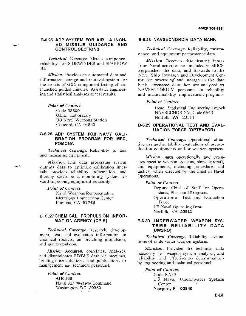
AMCP 706-196

B-6.25 ADP SYSTEM FOR AIR LAUNCH- ED MISSILE GUIDANCE AND CONTROL SECTIONS

Technical Couerage. Missile component reliability for SIDEWINDER and SPARROW III.

Mission. Provides an automated data and information storage and retrieval system for the results cf G&C component testing of air- launched guided missiles. Assists in engineering and statistical analyses of test results.

Point of Contact. Code 32300 QEE. Laboratory US Naval Weapons Station Concord, CA 94520

B-6.26 ADP SYSTEM FOR NAVY CALI- BRATION PROGRAM FOR MEC, POMONA

Technical Couerage. Reliability of test and measuring equipment.

Mission. This data processing system outputs data to optimize calibration intervals, provides reliability information, and thereby serves as a monitoring system toward improving equipment reliability.

Point of Contact, Naval Weapons Representative Metrology Engineering Center Pomona, CA 91766

B-6.27CHEMICAL PROPULSION INFOR- MATION AGENCY (CPIA)

Technical Coverage. Research, development, test, and evaluation information on chemical rockets, air breathing propulsion, and gun propulsion,

Mission. Acquires, correlates, analyzes, and disseminates RDT&E data via meetings, briefings, consultations, and publications to management and technical personnel.

Point of Contact. AIR-330 Naval Air Systems Command Washington, DC 20360

B-6.28 NAVSECNORDIV DATA BANK

Technical Coverage. Reliability, maintenance, and equipment performance data.

Mission. Receives data-element inputs from Naval activities not included in MDCS, keypunches the data, and forwards to the Naval Ship Research and Development Cen- ter for processing* and storage in the data bank. Processed data then are analyzed by NAVSECNORDIV personnel in reliability and maintainability improvement programs.

Point of Contact.

Head, Statistical Engineering Branch NAVSECNORDIV, Code 6643 Norfolk, VA 23511

B-6.29 OPERATIONAL TEST AND EVAL- UATION FORCE (OPTEVFOR)

Technical Couerage. Operational effectiveness and suitability evaluations of preproduction equipments and/or weapon systems.

Mission. Tfests operationally and evaluates specific weapon systems, ships, aircraft, and equipments, including procedures and tactics, when directed by the Chief of Naval Operations.

Point of Contact. Deputy Chief of Staff for Opera-

tions, Plans and Programs Operational Test and Evaluation

Force US Naval Operating Base Norfolk, VA 23511

B-6.30 UNDERWATER WEAPON SYS- TEMS RELIABILITY DATA (UWSRO)

Technical Coverage, Reliability evaluations of underwater weapon systans.

Mission. Provides the technical data necessary for weapon system analyses, and reliability and effectiveness determinations by engineering and technical personnel.

Point of Contact. Code RA32 U S Naval Underwater Systems

Center Newport, RI 02840

B-13

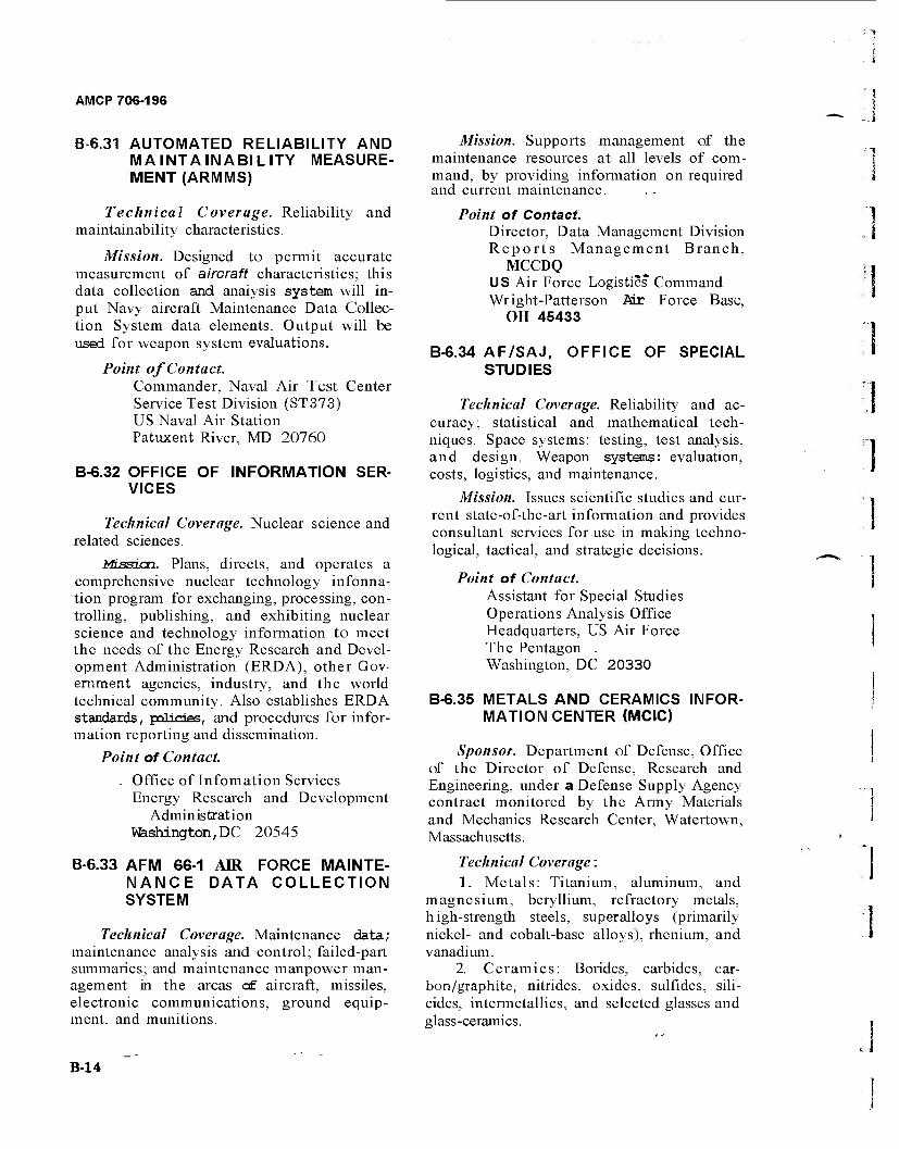
AMCP 706-196

B-6.31 AUTOMATED RELIABILITY AND MAINTAINABILITY MEASURE- MENT (ARMMS)

Technical Coverage. Reliability and maintainability characteristics.

Mission. Designed to permit accurate measurement of aircraft characteristics; this data collection and analysis system will input Navy aircraft Maintenance Data Collec- tion System data elements. Output will be used for weapon system evaluations.

Point of Contact. Commander, Naval Air Test Center Service Test Division (ST373) US Naval Air Station Patuxent River, MD 20760

B-6.32 OFFICE OF INFORMATION SER- VICES

Technical Coverage. Nuclear science and related sciences.

MLssicn. Plans, directs, and operates a comprehensive nuclear technology infonna- tion program for exchanging, processing, controlling, publishing, and exhibiting nuclear science and technology information to meet the needs of the Energy Research and Devel- opment Administration (ERDA), other Gov- ernment agencies, industry, and the world technical community. Also establishes ERDA standards, polides, and procedures for information reporting and dissemination.

Point of Contact.

. Office of Infomation Services Energy Research and Development

Administration Washington,DC 20545

B-6.33 AFM 66-1 AIR FORCE MAINTE- NANCE DATA COLLECTION SYSTEM

Technical Coverage. Maintenance data; maintenance analysis and control; failed-part summaries; and maintenance manpower management in the areas cf aircraft, missiles, electronic communications, ground equipment, and munitions.

Mission. Supports management of the maintenance resources at all levels of command, by providing information on required and current maintenance.

Point of Contact. Director, Data Management Division Reports Management Branch.

MCCDQ US Air Force Logistics Command Wright-Patterson Air Force Base,

OH 45433

B-6.34 AF/SAJ, STUDIES

OFFICE OF SPECIAL

Technical Coverage. Reliability and accuracy; statistical and mathematical techniques. Space systems: testing, test analysis, and design. Weapon systems: evaluation, costs, logistics, and maintenance.

Mission. Issues scientific studies and current state-of-the-art information and provides consultant services for use in making technological, tactical, and strategic decisions.

Point of Contact. Assistant for Special Studies Operations Analysis Office Headquarters, US Air Force The Pentagon . Washington, DC 20330

B-6.35 METALS AND CERAMICS INFOR- MATION CENTER {MCIC)

Sponsor. Department of Defense, Office of the Director of Defense, Research and Engineering, under a Defense Supply Agency contract monitored by the Army Materials and Mechanics Research Center, Watertown, Massachusetts.

Technical Coverage: 1. Metals: Titanium, aluminum, and

magnesium, beryllium, refractory metals, high-strength steels, superalloys (primarily nickel- and cobalt-base alloys), rhenium, and vanadium.

2. Ceramics: Borides, carbides, carbon/graphite, nitrides, oxides, sulfides, sui- cides, intermetallics, and selected glasses and glass-ceramics.

B-14

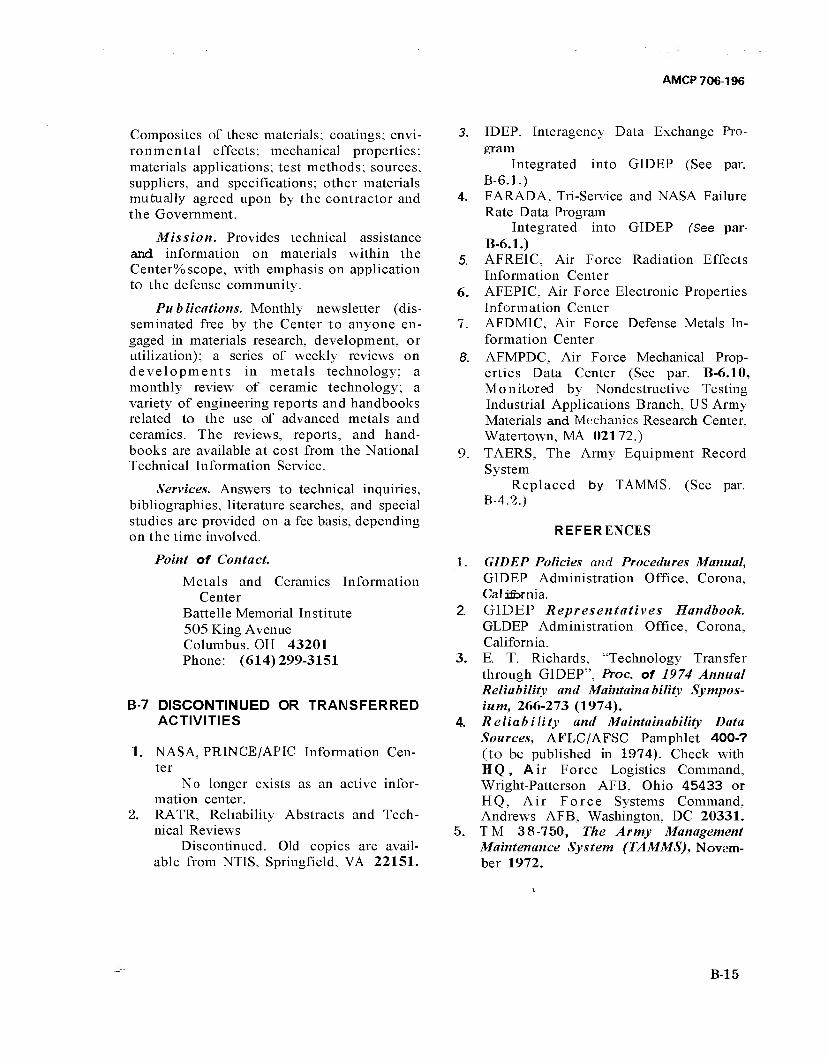
AMCP 706-196

Composites of these materials; coatings; environmental effects; mechanical properties; materials applications; test methods; sources, suppliers, and specifications; other materials mutually agreed upon by the contractor and the Government.

Mission. Provides technical assistance and information on materials within the Center% scope, with emphasis on application to the defense community.

Publications. Monthly newsletter (disseminated free by the Center to anyone en- gaged in materials research, development, or utilization); a series of weekly reviews on developments in metals technology; a monthly review of ceramic technology; a variety of engineering reports and handbooks related to the use of advanced metals and ceramics. The reviews, reports, and handbooks are available at cost from the National Technical Information Service.

Services. Answers to technical inquiries, bibliographies, literature searches, and special studies are provided on a fee basis, depending on the time involved.

Point of Contact.

Metals and Ceramics Information Center

Battelle Memorial Institute 505 King Avenue Columbus, OH 43201 Phone: (614)299-3151

B-7 DISCONTINUED OR TRANSFERRED ACTIVITIES

1. NASA, PRINCE/APIC Information Cen- ter

No longer exists as an active information center.

2. RATR, Reliability Abstracts and Tech- nical Reviews

Discontinued. Old copies are available from NTIS, Springfield, VA 22151.

3. IDEP, Interagency Data Exchange Pro- gram

Integrated into GIDEP (See par. B-6.1.)

4. FARADA, Tri-Service and NASA Failure Rate Data Program

Integrated into GIDEP (See par- B-6.1.)

5. AFREIC, Air Force Radiation Effects Information Center

6. AFEPIC, Air Force Electronic Properties Information Center

7. AFDMIC, Air Force Defense Metals In- formation Center

8. AFMPDC, Air Force Mechanical Prop- erties Data Center (See par. B-6.10, Monitored by Nondestructive Testing Industrial Applications Branch, US Army Materials and Mechanics Research Center, Watertown, MA 02172.)

9. TAERS, The Army Equipment Record System

Replaced by TAMMS. (See par. B-4.2.)

REFERENCES

1. GIDEP Policies and Procedures Manual, GIDEP Administration Office, Corona, California.

2. GIDEP Representatives Handbook. GLDEP Administration Office, Corona, California.

3. E. T. Richards, "Technology Transfer through GIDEP", Proc. of 1974 Annual Reliability and Maintainability Sympos- ium, 266-273 (1974).

4. Reliability and Maintainability Data Sources, AFLC/AFSC Pamphlet 400-? (to be published in 1974). Check with HQ, Air Force Logistics Command, Wright-Patterson AFB, Ohio 45433 or HQ, Air Force Systems Command, Andrews AFB, Washington, DC 20331.

5. TM 38-750, The Army Management Maintenance System (TAMMS), Novem- ber 1972.

B-15

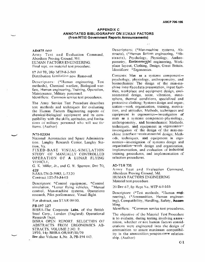
AMCP 706-196

APPENDIX C ANNOTATED BIBLIOGRAPHY ON HUMAN FACTORS

(from NTIS Government Reports Announcements)

AD-875 669 Army Test and Evaluation Command, Aberdeen Proving Ground, Md. HUMAN FACTORS ENGINEERING. Final rept. on materiel test procedure.

17 Jul 70, 26p MTP-8-3-509 Distribution Limitation now Removed.

Descriptors: (*Human engineering, Test methods), Chemical warfare, Biological warfare, Human engineering, Training, Operation, Maintenance, Military personnel. Identifiers: Common service test procedures.

The Army Service Test Procedure describes test methods and techniques for evaluating the Human Factors Engineering aspects of chemical-biological equipment and its compatibility with the skills, aptitudes, and limitations of military personnel who will use the items. (Author)

N71-12334 National Aeronautics and Space Administra- tion. Langley Research Center, Langley Sta- tion, Va. FIXED-BASE VISUAL-SIMULATION STUDY OF MANUALLY CONTROLLED OPERATION OF A LUNAR FLYING VEHICLE. G. K. Miller, Jr., and G. W. Sparrow. Dec 70, 42P NASA-TN-D-5983, L-7320 Contract 127-51-34-03

Descriptors: *Control equipment, *Control simulation, *Lunar flying vehicles, "Manual control, Man-machine systems, Operations research, Pilot performance, Visual flight.

For abstract, see STAR 09 03.

PB-197 127 BISRA-The Corporate Labs, of the British Steel Corp., London (England). Operational Research Dept. BISRA OPEN REPORT. SELECTION OF ABSTRACTS FROM ERGONOMICS AB- STRACTS, VOLUME 2 NO. 2. 1970, 14p BISRA-OR/HF/35/70 See also Volume l,No. 3, PB-194 443.

Descriptors: (*Man-machine systems, Ab- stracts), (*Human factors engineering, *Ab- stracts), Psychology, Physiology, Anthro- pometry, Environmental engineering, Work- place layout, Clothing, Design, Great Britain. Identifiers: * Ergonomics.

Contents: Man as a systems component— psychology, physiology, anthropometry, and biomechanics: The design of the man-machine interfacedata presentation, input facilities, workplace and equipment design, environmental design, noise, vibration, atmosphere, thermal conditions, specialized and protective clothing; Systems design and organ-, ization—work organization, training, motivation, and attitudes; Methods, techniques and equipment in ergonomics—investigation <£ man as a systems component-physiology, anthropometry, and biomechanics; Methods, techniques, and equipment in ergonomics- investigation of the design of the man-machine interface—environmental design; Meth- ods, techniques, and equipment in ergonomics—investigation of systems design and organization—work design and organization, implementation, and evaluation of industrial training procedures, and implementation of selection procedures.

AD-718 731 Army Test and Evaluation Command, Aberdeen Proving Ground, Md. HUMAN FACTORS ENGINEERING Materiel test procedure.

20 Dec 67, 5p Rept No. MTP-4-3-515

Descriptors: (*Test methods, *Human engineering), (*Ammunition, Human engineering), Compatibility, Handling, Safety, Assart bling. Identifiers: *Common service test procedures.

The objective of the Materiel Test Procedure is to evaluate, during testing involving ammunition, whether or not human factors considerations were engineered into the design of ammunition to assure maximum compatibility in the ammunition-weapon-crew relationship. (Author)

C-l

AMCP 706-196

AD-732 613 Illinois Univ. Savoy Aviation Research Lab. EFFECTS OF THE MAN ON THE TASK IN COMPLEX MAN-MACHINE SYSTEMS, Charles L. Hulin, and Kenneth M. Alvares. Feb 71, 14p AFHRL-TR-71-7 Contract F41609-7 O-C-0027 See also related reports AD-731 191 and AD-732 612.

Descriptors: (* Man -machine systems, *Job analysis), Training, Factor analysis, Design, Effectiveness. Identifiers: Pilot training.

This research tested the hypothesis that in a complex man-machine system, one of the many influences on the system is the man's constant reorganization of the tasks which constitute the system. The performances of 67 male college students receiving basic flight training were assessed by means of check rides at three different points of training. Factor analyses of each set of check ride data indicated systematic changes occurred in the structure of the task. A three-factor solution appeared in the 10-hour data, two factors were being assessed by the 25-hour point, and only one general factor appeared in the 35-hour data. This finding indicates that future man-machine systems research should no longer be designed under a fixed-task as-

1 sumption. It is speculated that this assumption may be one cause of the generally found weak prediction of system performance effectiveness over meaningful intervals of time (Author)

AD-721 657 Dunlap and Associates Inc., Darien, Conn. HUMFACTS SYSTEM THESAURUS.

Jan 71,419p* Contract DAHC04-69-C-0076

Descriptors: (* Dictionaries, *Human engineering), Information retrieval, Vocabulary, Subject indexing.

Identifiers: *Thesauri. HUMFACTS System Thesaurus.

The thesaurus cxntains words and phrases, concept-terms, which reflect the concepts to be indexed in support of the Human Factors, Engineering Information Retrieval (HUM-

c-2

FACTS) System. The concept-terms indicate structures which display the relationship between terms to at least two levels of detail in meaning. This developmental thesaurus is intended to serve as the authority list for subsequent indexing and retrieval processing but is not considered final. (Author)

AD-730 910 Bunker-Ramo Corp., Westlake Village, Calif. DEVELOPMENT OF A HUMAN PERFOR- MANCE RELIABILITY DATA SYSTEM. Technical rept., David Meister, and Robert G. Mils. Jun 71, 19p AMRL-TR-71-74

Contract F33615-70-C-1518 Presented at the Reliability and lyfeintain- ability Conference (10th), held on 28-30 Jun 71.

Descriptors: (*Performance (Human), *Reli- ability), (*Behavior, Classification). Man-machine systems, Data, Human engineering. Feasibility studies. Identifiers: Taxonomy.

A study was performed to determine the requirements for and the elements of a human performance reliability (HPR) data system. The heart of the HPR system is a taxonomic structure for classifying behavioral studies. 140 studies from a variety of sources were coded using this taxonomy. To test the effi- ciency of this databank to provide answers to syslfcui development questions, a number of tests were performed to determine the relevance of the data retrieved to the questions asked. The results of these tests indicated that it is possible to expand the HPR data base provided one is not restricted to a probabilistic metric. (Author)

AD-730 923 Michigan Univ., Ann Arbor Human Perform- ance Center SHORT-TERM MEMORY FOR QUANTI- TATIVE INFORMATION FROM THREE KINDS OF VISUAL DISPLAYS. Technical rept., Vicki Vivienne Rhona Cohen. Jun 71, 89p Rept Nbs. 08773-82-T, TR-28 AFOSR-TR- 71-2580 Contract AF 49(638)-1736, ARPA Order-461

,j

AMCP 706-196

Descriptors: (*Memory, Display systems), Human engineering, Recall, Motion. Identifiers: Short term memory.

A series of four experiments was conducted to investigate whether the nature of a visual display affects short-term memory for numer- ic information extracted from it. Three different kinds of displays were chosen for study: a digital counter, a moving scale, and a moving pointer display. Experiment I examined reading performance using the moving scale and moving pointer displays. The results of this experiment, in which the moving scale yielded superior performance, provided base- line data with which to judge future performance and also enabled a judicious choice of exposure durations for the subsequent experiments. In Experiment II the Brown-Peterson paradigm with vaned retention intervals was used to examine the short-term memory for quantitative information from the three kinds of displays. In general, the digital counter yielded the best recall performance, followed by the moving pointer and moving scale displays in that order. Experiments III and IV were between- and within-in subjects designs which tested this hypothesis using the Brown-Peterson paradigm with two different interpolated tasks, one of which interfered with the retention of verbal information and the other which interfered with the retention of both verbal and nonverbal information. The differences in error patterns obtained in Experiment II between the moving pointer and moving scale displays were again obtained when the interpolated activity was considered to be causing only verbal interference. How- ever, this difference was abolished or considerably lessened when the interpolated activity was one that interfered with both verbal and nonverbal memory. (Author)

AD-729 855 Army Test and Evaluation Command, Aberdeen Proving Ground, Md. HUMAN FACTORS ENGINEERING Final rept. on materiel test procedure. 1 Sep 71, 22p Rept. No. MTP-10-2-505 Supersedes Rept. No. MTP-10-2-505 dated 19 Jul 67, AD-725 555.

Descriptors: (*Army equipment, Human engineering), (*Human engineering, Test methods), Measurement, Standards, Accu- racy, Errors, Performance (Engineering), Per- formance (Human), Safety. Identifiers: * Common engineering test procedures.

The document outlines procedures for evaluating the human factors associated with use of general equipment. (Author)

AD-729 964 Texas Tech Univ., Lubbock Center of Bio- technology and Human Performance. PERFORMANCE, RECOVERY AND MAN- MACHINE EFFECTIVENESS. Semi-annual progress Rept. 1 Mar—31 Aug 71, Richard A. Dudek. 15 Sep 71, 26p Contract DAAD05-69-C-0102 See also Seminannual progress rept. dated 1 5 Mar 71,AD-723 430.

Descriptors: (*Man-machine systems, Effec- tiveness). (*Performance (Human), Environ- ment), Stress (Psychology), Stress (Physiol- ogy), Behavior, Attention, Motivation, Nutri- tion, Vibration, Climatology, Exercise, Rhythm (Biology), Fatigue (Physiology), Group dynamics, Military personnel.

The goals of the research are the determination of optimal or near optimal work/rest schedules for individuals and crews to yield high performance with minimal decrement overtime followed by recovery (after rest) to an acceptable high performance. The experimentation is further aimed at consideration of various task levels and differing conditions of environment. Experimentation in progress continues to focus attention on the assessment of human performance under continuous operations or relatively long term activity (2 hours or more of activity). Effects of circadian rhythms on performance will also be studied in connection with this project.

AD-' 125 555 Army Test and Evaluation Command, Aberdeen Proving Ground, Md.. HUMAN FACTORS EVALUATION Materiel test procedure.

c-3

AMCP 706-196

19Jul 67, 8p Rept. No. MTP-10-2-505

Descriptors: *Army equipment, Human engineering), (*Human engineering, Test methods), Test facilities, Questionnaires, Tech- nicians, Personnel management. Identifiers: *Common engineering test procedures.

The objective of the materiel test procedure is to provide general testing procedures to be used in conducting the human factors portion of engineering tests of general supplies and equipment, and to evaluate the human factors requirements of the test items as set forth in QMR's, SDR's, technical characteristics, and as indicated by the particular design. These procedures are to be used along with other engineering test procedures to determine the technical and maintenance suitability of the test items for service tests. (Author)

AD-719 108 Army Test and Evaluation Command, Aberdeen Proving Ground, Md. HUMAN FACTORS. Final rept. on materiel test procedure. 11 Dec 70, 22p Rept no. MTP-7-3-510

Descriptors: ("Human engineering, Test methods), Test equipment, Noise, Visibility, Environment, Military facilities, Control systems, Display systems, Installation, Reli- ability, Maintenance, Safety, Data processing systems. Identifiers: Evaluation, * Common engineering test procedures, "Avionics.

Human factor considerations applicable to aviation armament and avionics are described. (Author)

AD-727 658 Human Resources Research Organization, Alexandria, Va MAN IN CONTROT OF FflGHTY AUTO- MATED SYSTEMS Harry L. Ammerman, and William H. Melching. May 71, 14p *Rept No. HUMRRO professional paper 7-71 Contract DAHC19-70-C-0Ö12 Presented at the. Annual Army Human Fac- tors Research and Development Conference (leth). Ebrt Bliss, Texas Oct 70.

Descriptors: (^Performance (Human), Com- mand + control systems), (* Automation,

*Man-machine systems), Control panels, Decisionmaking, Reliability, Human engineering, Factor analysis. Identifiers: * Highly automated*systems.

The identification of what man should do as a decisionmaker and controller in the newly evolving man-machine systems is considered. Among the topics discussed "Jure man's underlying basic functions in a complex system, task activities for individual jobs and their analyses, and training and the design of operational job positions. (Author)

AD-728 099 Human Resources Research Organization, Alexandria, Va. SURVEY OF FACTORS INFLUENCING ARMY LOW LEVEL NAVIGATION. Technical rept., Robert H. Wright, and Warren P. Pauley, Jun 71,125p Rept No. H Contract DAHC19-70-C-0012

Descriptors: (^Navigation, Low altitude), (*:Human engineering, Navigation), Display systems, Navigation computers, Army training, Human engineering. Performance (Hu- man), Mssion profiles, T?=rrain, Climatology. Identifiers: Low level navigation.

Factors that influence low level navigation and affect Army capability in conducting low level missions were surveyed. The nation of improvements in equipment, procedures, and training needed to provide the Army with effective operational capability in low level navigation were indicated, Jfejor conclusions from the survey include limited capability in low level aerial navigation as affecting future Army combat effectiveness; the rapid reaction mission over unfamiliar terrain in low level navigation; pcteifcial improvements in training or procedures for present navigation system and equipment; a simple automatic dead reckoning navigation computer in routine attainment of operationally effective low level navigation performance; and reorienting navigation procedures and training to simplified line of position navigation techniques. (Author)

C-4

AMCP 706-196

AD-717 257 Human Resources Research Organization, Alexandria, Va COLLECTED PAPERS PREPARED UNDER WORK UNIT REPAIR. TRAINING OF ELECTRONICS MAINTENANCE PER- SONNEL.

Nov 70, 41p ReptNo.HUMRRO professional paper-27-70 Contract DAHC19-70-C-0012

Descriptors: (* Maintenance personnel, *Army training), ("Radio receivers, Maint- enance), Teaching methods, Radio communication systems, Sequences, Malfunctions, Cir- cuits, Theory. Identifiers: *Field radio repair courses, Troubleshooting, REPAIR work unit.

Papers in the collection report research in procedures in troubleshooting and repair of Army field radios that resulted in the construction of evaluations of the men and in experimental training courses. The papers are: The implementation of functional context training in a radio repairman course; A follow-up study of experimentally trained and conventionally trained field radio repairmen; REPAIR III: The development and evaluation of the experimental field radio repairman course; REPAIR IV: Comparison of experimental and standard course graduates after field experience. (Author)

AD-717 258 Human Resources Research Organization, Alexandria, Va. AN APPROACH TO STANDARDIZING HUMAN PERFORMANCE ASSESSMENT. John D. Engel. Oct 70, 14p *Rept No. HUMRRO-professional paper-26-70 Contract D AHC19-7 O-C-0012 Presented at the Planning Conference of 'Standardization of Tasks and Measures for Human Factors Research', held at Texas Technological Univ., Lubbock, Tex., Mar 70.

Descriptors: (*Performance (Human), Meas- urement), (*Test construction (Psychology), Standardization), (*Performance tests, Stand- ardization), Test methods, Visual acuity, Auditory acuity, Decisionmaking, Symbols, Documentation.

Identifiers: Evaluation, Task analysis, Tax- onomy, Manipulation.

The standardization and evaluation of methods of performance assessment represents an important area of concern. In this paper an approach that concentrates on two critical areas and the relationship between them is discussed. TJiese are: (a) a task classification system, and (b) a performance measure classification system. An example is presented that illustrates some preliminary research related to the use of a performance measure classification system. The paper con- cludes by suggesting areas and directions for future research efforts. (Author)

AD-720 354 Applied Psychological Services Inc., Wayne, Pa. Science Center DIGITAL SIMULATION OF THE PERFOR- MANCE OF INTERMEDIATE SIZE CREWS : APPLICATION AND VALIDATION OF A MODEL FOR CREW SIMULATION. Technical rept., Arthur I. Siegel, J. Jay Wolf, and Joseph Cosentino. Feb 71, 157p *Rept No. APS-7071-5 Contract N000 14-68-C-0262

Descriptors: (*Naval personnel, Performance (Human)), (* Man -machine systems, Mathe- matical models), Organizations, Curve fitting, Mathematical prediction, Programming (Com- puters), Digital computers, Simulation, Mili- tary psychology, Mission profiles, Correlation techniques, Data processing systems, Vietnam. Identifiers: Computerized simulation, Evalua- tion

Based on current psychological theory, nüt tary doctrine, and previously developed and tested functional relationships, selected psychosocial, personnel, and performance variables are woven into a stochastic mathematical model for digitally simulating closed man-machine systems operated by crews of from 4 to 20 members. This probabilistic model is presented in terms cf a detailed logic and processing flow sequence. An operational mission (Vietnam river patrol) selected for the evaluation of the model is then described and

c-5

AMCP 706-196

quantified as required for input to the model. The results of a series of evaluative simulation runs, in which the computer simulation model is applied to the mission, are reported. These results are compared with independent criterion data for the same mission. (Author)

AD-720 976 Army Test and Evaluation Command, Aberdeen Proving Ground,Md. HUMAN FACTORS ENGINEERING. Materiel test procedure.

27 Aug 69, 70p Rept No.MTP-6-2-502

Descriptors: (*Human engineering, Test methods), (*Man-machine systems, Human engineering), Display systems, Control panels, Warning systems, Auditory perception. Identifiers: Common engineering test procedures, Auditory warning devices, Visual displays.

The objective of the Materiel Test Procedure is to provide methods of determining the appropriateness and effectiveness of human factors aspects at man-machine interfaces. (Author)

AD-726 306 Aerospace Medical Research Lab, Wright- Paterson AFB, Ohio HUMAN FACTORS AND SYSTEMS EFFEC- TIVENESS. Donald A Topmiller. 1966, lip Rept No. AMRL-TR-66-257 Presented at the Reliability and Maintain- ability Conference (5th) held on 18-20 Jul 66. Availability: Pub. in Annals of Reliability and Maintainability, v5 p!23-132, 1966.

Descriptors: (*Performance (Human), Effec- tiveness), (*Human engineering, Mainte- nance), Systems engineering, Reliability, Maintainability, Mathematical prediction, Statistical analysis, Errors, Time,

The paper treats human factors in systems effectiveness as" a basic problem relating human performance to the major Systems effectiveness parameters of operability, reliability, and maintainability. The latter two parameters are topologically related to the primary dependent human performance variables used in laboratory research of errors and

time respectively. The need is outlined to not only topologically relate these variables but to also develop a framework within which human engineering design can be quantitatively assessed. Two studies weite reviewed in which human performance (time) was predicted from design evaluations and analysis of equipment. (Author)

AD-877 006

Naval Missile Center, Point Mugu, Calif. DYNAMIC TARGET IDENTIFICATION ON TELEVISION AS A FUNCTION OF DIS- PLAY SIZE, VIEWING DISTANCE, AND TARGET MOTION RATE. Technical publications, R. A. Bruns, R. J. Wherry, Jr., and A. C. Bittner, Jr., 17Nov 70, 64p NMC-TP-70-60 Distribution Limitation now Removed.

Descriptors: ("Closed circuit television, De- sign), (* Target acquisition, Closed circuit television), (*Naval aircraft, Closed circuit television), Human engineering, Accuracy, Tele- vision display systems, Ranges (Distance), Motion, Electrooptics, Air-to-surface, Simula- tion, Tactical warfare. Identifiers: *Reconnaissance transparency projection systems, * Airborne television systems.

The report describes the results of a research study whose goal was the evaluation of the effects of (1) television display size, (2) display degradation, (3) observer viewing distance, and (4) target motion rate on target identification performance. Appendixes to the report describe (1) a reconnaissance transparency projection system used to simulate the televisual air-to-surface tactical target attacks used as test materiel in this study and (2) a rating procedure used to compare target briefing photographs in terms of qualities important for target identification. The target ratings are then used to predict target identification performance in the simulated target attacks. (Author)

JPRS-53244 Joint Publications Research Service, Wash- ington, D.C. INFORMATION CHARACTERISTICS OF DISPLAY SYSTEMS AND THEIR RELA- TIONSHIP TO PSYCHOPHYSIOLOGICAL

1

I

C-6

AMCP 706 196

INDICATORS OF OPERATOR ACTIVITY Yu. A. Ivashkin. 28 May 71, 13p Trans, of Pribory i Sistemy Upravleniya (USSR)-4,p22-25, 1969.

Descriptors: (*Display devices, Information systems), Computer storage devices, Mathe- matical models, Information theory, Infor- mation capacity, Senses, Visual perception.

N71-23210 Advisory Group for Aerospace Research and Development, Paris (France). FREQUENCY RESPONSE FUNCTIONS AND HUMAN PILOT MODELLING. Mar 71, 65p AGARD-R-580-71 Lang—Mostly in English, Partly in French

Descriptors: * Aircraft structures, Dynamic response, *Dynamic structural analysis, * Human factors engineering, "Mathematical models, *Pilot performance, *Transfer functions, Frequency response, Functional analysis, Gusts, Modal response. Identifiers: NASA subject code 01.

For abstract, see STAR 0912.

AD-727 365 Aerospace Medical Research Lab, Wright- Paterson AFB, Ohio. HUMAN FACTORS ENGINEERING CON- SIDERATIONS IN SYSTEM DEVELOP- MENT Julien M. Christensen. 1969, 33p Rept No. AMRL-TR-69-82 Availability: Pub. in Proceedings of the DRG Seminar on Design of Equipment for Effec- tive Utilization (5th), 21-23 Sep 69, P113-144.

Descriptors: (*Human engineering, "Systems engineering), Design.

The purpose of the paper is fourfold. First, the life cycle in the design and development of a typical system is described. Second, the nature of human factors engineering requirements is described. Third, these requirements are related to the systems development cycle and, finally, a brief evaluation will be made c£ the tools and information available to the human factors engineer. (Author)

N71-25943 Man Factors, Inc., San Diego, Calif. DATA BOOK FOR HUMAN FACTORS ENGINEERS. VOLUME 2 - COMMON FORMULAS, METRICS, DEFINITIONS. C. Kubokawa, P. Selby, andW. Woodson, Nov 69, 371p NASA-CR-114272 Contract NAS2-5298

Descriptors: *Conv5rsion tables, *Formulas (mathematics), *Human factors engineering, *Nomenclatures, Manuals, Nomographs, Symbols, Units of measurement.

For abstract, see STAR 09 14.

N71-25944 Man Factors, Inc., San Diego, Calif. DATABOOK FOR HUMAN FACTORS EN- GINEERS. VOLUME 1 - HUMAN ENGI- NEERING DATA. C. Kubokawa, P. Selby, and W. Woodson, Nov 69, 260p NASA-CR-114271 Contract NAS2-5298

Descriptors: * Anthropometry, *Environmen- tal index, * Human behavior, * Human factors engineering, * Physiological factors, Equip- ment specifications, Graphs (charts), Manuals, Tables (data). For abstract, see STAR 09 14.

N7 1-26160 Bolt, Beranek, and Newman, Inc., Cambridge, Mass. STUDIES OF MULTIVARIABLE MANUAL CONTROL SYSTEMS - A MODEL FOR TASK INTERFERENCE. J. I. Elkind, W. H. Levison, and J. L. 'Word. May 71, 229p NASA-CR-1746 Contract NAS2-3080 Coll- 229P Refs

Descriptors: *Manual control, *Mathemati- cal models, * Pilot performance, *Task complexity, Display devices, Man-machine systems, Performance prediction, Tracking (position). For abstract, see STAR 09 14.

AD-727 254 McDonnell Douglas Corp., Long Beach, Calif, Douglas Aircraft Div.

C-7

AMCP 706-196

-?

WHAT'S WRONG WITH HUMAN FACTORS IN SYSTEMS DEVELOPMENT AND HOW CAN THIS BE CORRECTED Arthur S. Romero. 1 Sep 68, 8p Rept No. Douglas Paper-5208

Descriptors: (*Human engineering, Man-machine systems), Systems engineering, Problem solving, Philosophy, Documentation, Factor analysis, Effectiveness.

Problems of design, development and maintenance of sophisticated systems have brought forth a specialized approach to information about man known as human factors. Observa- tion of design and development of systems and subsystems from the conceptual phase to mockup review reveals some of the underlying causes for the failure to incorporate human factors into the design. These causes and some recommendations for eliminating them from future design are discussed. (Author)

C-8

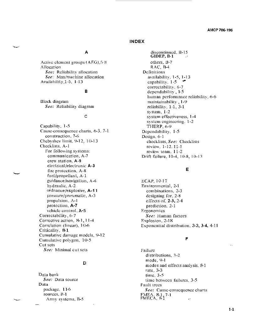
INDEX

AMCP 706-196

Active element groups (AEG),5-8 Allocation

See: Reliability allocation See: Man/machine allocation

Availability,1-5, 1-13

B

Block diagram See: Reliability diagram

Capability, 1-5 Cause-consequence charts, 6-3, 7-1

construction, 7-6 Chebyshev limit, 9-12, 10-13 Checklists, A-l

For following systems: communication, A-7 crew station, A-9 electrical/electronic A-3 fire protection, A-8 fuel/propellant, A-l guidance/navigation, A-6 hydraulic, A-2 ordnance/explosive, A-1 1 pressure/pneumatic, A-3 propulsion, A-l protection, A-7 vehicle control, A-5

Correctability, 6-7 Corrective action, 8-1,11-4 Correlation (linear), 10-6 Criticality, 8-1 Cumulative damage models, 9-12 Cumulative polygon, 10-5 Cut sets

See: Minimal cut sets

discontinued, B-15 GIDEP, Bl

others, B-7 RAC, B-4

Definitions availability, 1-5, 1-13 capability, 1-5 "'* correctability, 6-7 dependability , 1-5 human performance reliability, 6-6 maintainability , 1 -9 reliability, 1-1, 3-1 system, 1-2 system effectiveness, 1 -4 system engineering. 1-2 THERP, 6-9

Dependability, 1-5 Design, 6-1

checklists, See: Checklists review, 1-12,11-1 review team, 11-2

Drift failure, 10-4, 10-8, 10-13

Data bank See: Data source

Data package, 11-6 sources, B-l

Army systems, B-5

ECAP, 10-17 Environmental, 2-1

combinations, 2-3 designing for, 2-8 effects of, 2-3, 2-4 prediction, 2-1

Ergonomics See: Human factors

Explosion, 2-18 Exponential distribution, 3-3, 3-4, 4-11

Failure distributions, 3-2 mode, 9-1 modes and effects analysis, 8-1 rate, 3-3 time, 3-5 time between failures, 3-5

Fault trees See: Cause-consequence charts

FMEA, 8-1,7-1 FMECA, 8-1

1-1

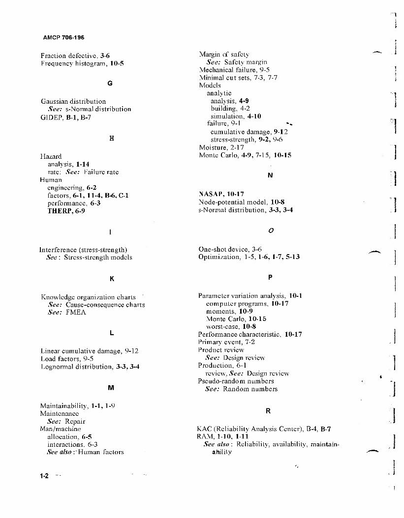
AMCP 706-196

Fraction defective, 3-6 Frequency histogram, 10-5

Gaussian distribution See: s-Normal distribution

GIDEP, B-l, B-7

H

Hazard analysis, 1-14 rate: See: Failure rate

Human engineering, 6-2 factors, 6-1, 11-4, B-6, C-l performance, 6-3 THERP,6-9

Margin cf safety See: Safety margin

Mechanical failure, 9-5 Minimal cut sets, 7-3, 7-7 Models

analytic analysis, 4-9 building, 4-2 simulation, 4-10

failure, 9-1 cumulative damage, 9-12 stress-strength, 9-2, 9-6

Moisture, 2-17 Monte Carlo, 4-9, 7-15, 10-15

N

NASAP, 10-17 Node-potential model, 10-8 s-Normal distribution, 3-3, 3-4

— .1

Interference (stress-strength) See: Stress-strength models

One-shot device, 3-6 Optimization, 1-5, 1-6, 1-7, 5-13

K

Knowledge organization charts See: Cause-consequence charts See: FMEA

Linear cumulative damage, 9-12 Load factors, 9-5 Lognormal distribution, 3-3, 3-4

M

Parameter variation analysis, 10-1 computer programs, 10-17 moments, 10-9 Monte Carlo, 10-15 worst-case, 10-8

Performance characteristic, 10-17 Primary event, 7-2 Product review

See: Design review Production, 6-1

review, See: Design review Pseudo-random numbers

See: Random numbers

Maintainability, 1-1, 1-9 Maintenance

See: Repair Man/machine

allocation, 6-5 interactions, 6-3 See also :" Human factors

KAC (Reliability Analysis Center), B-4, B-7 RAM, 1 10, 1-11

See also : Reliability, availability, maintainability

1-2

AMCP 706-196

Random numbers, 4-10 Redundancy, 1-8, 4-3 REG (Reasonable Engineering Guess), 9-11,

10-13 Reliability

allocation, 5-1 systems with repair, 5-23 systems without repair, 5-2 nonredundant, 5-2, 5-3,5-8,5-9 redundant, 5-13, 5-20

block diagrams: See: Reliability diagram diagram, 4-2, 8-2 measures, 3-1

Repair, 1-8, 1-9

Safety, 1-1, 1-13 factors, 9-5 margin, 9-5, 9-11

Sand and dust, 2-17 Sensitivities, 10-14 Shock and vibration, 2-15 Simulation, 7-15 Stimulus, 6-4 Stress-strength models, 9-2, 9-6

deterministic, 9-2 probabilistic, 9-6

System definition, 7-6 effectiveness, 1-4, 6-2 engineering, 1-2 management, 1-2, 1-3, 6-2

Tails (of a distribution), 10-4 TAMMS, €3-5,B-8 ~ Task equipment analysis (TEA), 6-6, 6- Temperature, 2-14 Tensile strength, 9-2 THERP, 6-9 Top event, 7-2, 7-6 Trade-off, 1-1, 1-15,1-16, 6-6, 6-8

Variability analysis See: Parameter variation analysis

W

Weibull distribution, 3-3, 3-4 Worst case analysis, 10-8

1-3

(AMCRD-TV)

FOR THE COMMANDER:

AMCP 706-196

OFFICIAL: ROBERT L. KIRWAN Brigadiec»General, USA Chief of Staff

a^___

LTC, GS Adjutant General

DISTRIBUTION: Special

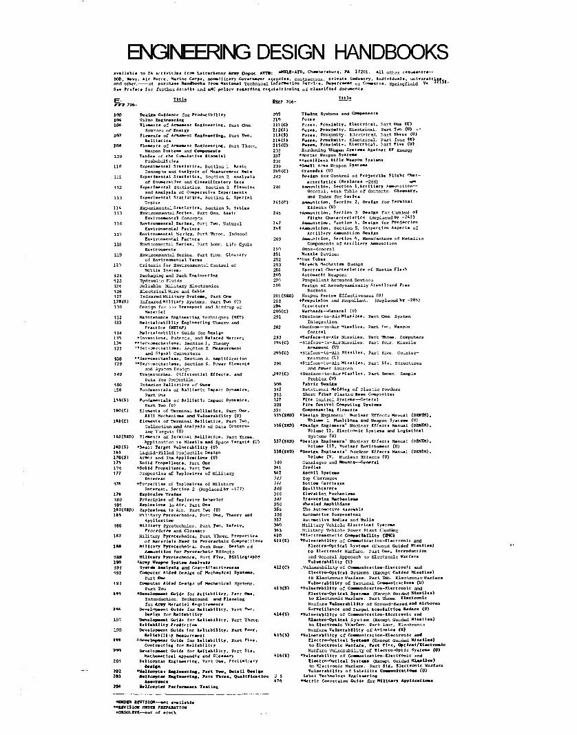
ENGINEERING DESIGN HANDBOOKS *v«ll«bl« to DA sctivitlas fro« L«tt«rk«nny Army Depot. ATTH: AKAXE-ATÜ. Ch*nfeersburg, PA 17201. All other renuastors-- 000, Ravy, Air Force, Karin« Corps, noomUttary Governacnt iênclt», contractors, privat* Industry, Individual», universities and other. at purchase Handbook« fro« «atIon« 1 Technical Information Service, Department 0f Commerce. Springfield. VA "lM- Se« Prefses for further dataila and AMC policy regarding requisitioning Qf classified document«.

Title Maep 706-

Title

100 in* 106

107

]OS

139

llfl

111

112

113

114 113

116

117

118

119

120

121 123 126 125 127 IZBfS) 130

132 133

134 135 13ft 131

138 139

150 153

IW(S)

160(C)

161(C)

163<S) 16} 170(S) 175 176 177

17»

179 180 181 1»2<SRD) 195

186

m

188

189 190 191 192

I'M.

197

198

199

TOO

201

Engineering» Part Two,

Engineering, Part Three,

»enc Rat*

Amplification Power Elements

201 203

Design Guidance for ProcHicibility Value Engineering Elemaat« of Armament Engineering, part One.

Sources of Energy Element« of *r

Ballistics Elemeot« of Ar

Weapon Syatem« and Component« Tablca of the CuauUti»« Binomial

Probabilities Experimental Sratlatlc», Section 1

Concepts and Analyai« of Heaau Experimental Statistic«, Section 2. Analyai*

of Enumeracive and Claaaiflcatory Data Experimental Statistics. Section 3. Planning

and Analysis of Comparative Experiment* Enperimental Statistics, Section L. Special

Topic* Experimental Statistic«, Section 5, Tables Environmental Serie«, Part One, Basic

Environmental Concepts Environment«! Series, Part Two, Natural

Environmental Factors Environmental Series. Part Three. Induced

Environmental Factor« Environmental Series, Part lour. Life Cycle

Environments Environmental Series. Part Five. Glossary

of Environmental Terms Criteria for Environmental Control of

Mobile S?«teas Packaging and Pack Engineering Hydraulic Fluids Reliable Military Electronics Electrical Wire and Cable InfraredMilitary Systems, Part One Infrared Military Systems. Part Two (U) Design for Air Transport and Airdrop of

Materiel Maintenance Engineering, techniques (MET) Maintainability Engineering Theory and

Practice (KETAP) Maintainability Guide for De*ign

♦Inventions, Patents, and Related Matters **Servoaechantsins, Section 1, Theory "•Servosseehanlsma, Section 2. Measurement

and Signal Converters '•ServoBechanlaae, Section 3. **S*rvoaecheoisaB, Section 6.

and System Design Trajectories. Differential Effects, and

Data for Projectile. Interior Ballistics of Gun« Fundamentals of Ballistic Impact Dynamics,

Part One Fundamental« of Ballistic Impact Dynamics,

Part Two (U) Element» of Terminal Ballistic«, Part One,

Kill Mechaalsme and Vulnerability (U) Element« of Terminal Balllatlca, Part Two,

Collection and Analyaie of Data Concern- ing Targets (U)

Elements of Terminal Ballistics, Part Three. Application to Hlssil« and Space Target« (U)

"Basic Target Vulnerability (0) Liquid-Filled Projectile Dealgn Armor and Ita Applications (0) Solid Fropellanta, Part One

♦-Solid Propellents, Part Two Propertlea of Explosive» of Military

Interest ♦Properties of Explosives of Military

Interest, Section 2 (Replacedby -177) Explosive Trains Principle« of Explosive Behavior Explosion« lo Air, Part One Explosion« In Air. Part Two (U) Military Pyrotechnics, Part One, Theory and

Application Military Pyrotechnics. Part Two, Safety,

Procedure« and Glossary Military Pyrotechnic«, Part Three. Properties

of Materials Haed lo Pyrotechnic Compositions Military Pyrotechnics, Part Pour. DeMgn of

Aastunlrloa for Pyrotechnic Effects Military Pymtechntc«, Part Five, Bibliography

«Army Weapon System Aoalyals System Analyst« and Coat-Eff«ctiveoeaa Computer Aided Design of Mechanical Sy«terns.

Part One Computer Aided Design of Mechanical Systems.

Part Two *Development Cut de for Reliability. Fart One,

Introduction. Background, and Planning for Army Materiel Requirements

Development Culd* for Reltablllty, Part Two. Öeslgn for JUIl-MUty

-Development Guide for ««liability, Part Three, »liability Prediction "Development Guide fnr Reliability, Part Four,

««liability Measurement •Bevelnpiant Guide for Reliability, Part Five,

Contracting for Reliability Development Guide for fceliabUtty, Part Six,

Mathematical Appendix and Glossary Belicoptar Engineering, Part On«, Preliminary

D*ai#;a •amllcomtar ■aujlnccxlna;. Fart Two. Detail Dee I go Bellcopter BnfloaerinA, Fart Tnraa, Quallficatio<

r Tracing

205 210 211<C> 212(S> 213(S) 214(S) 215(C> 233 237 238 239 240(C)

242

246

245(C)

246

247 248

250 251 252 253 255 2AO 270 2 SO

281(SRD) 282 266 290(C)

291

292

293 294(C)

295(C)

296

.297(C)

300 312 313 127 329 331 135 (SRD)

336(SRD)

337(SRD)

33«(SRD)

340 341 342 343 344 345 366 347 350 35s 356 357 360 36L 410 41l(S)

Timing Systems and Component« FuxeS

Part One (U> Part Two (U) *■> Part Three <U> Part four (D) Part Five (0)

Fuses, »roxialty. ElectTlcal, ruiei, Proximity, Electrical. Fuze«, Proximity. Electrical. Fuzes. ProKinitY-, Electrical. Fuie-i, Proxlitltv, Electric«!, Hardening Weapon Systems Agalnat RF Energy

•Mortar Weapon System« •Recoilles« Rifle Weapon Systems •Small Anas Weapon System« Grenades (U> De»ign for Control of Projectile Flight Char-

acteristics (Replaces -266) »» Ammunition, Section I,Artillery Ammunition—

General, with Table of Contents. Gloaaary. and Index for Series

Armunition, Section 2, Design for Terminal Effects (0)

♦Ansauntt ion. Section 3. Design for Control of Flight Characteristics (Replacedby -242)

Ammunition. Section 4, Design for Projection 4-Aanunition, Section 5, Inspection Aspect« of

Artillery Ammunition Design Amaunltion, Section 6, Manufacture of Metallic

Components of Artillery Ammunition Gun s-<eneral Hutile Devices

**0un Tubes •Breech Mechanism Design Spectral Characteristics of Hustle Flash Automatic Weapons Propellant Actuated Devices ftesign of Aerodynamically Srahilixed Free

Rockets Weapon Systen Effectiveness IV)

+Propul«ion and Propellant. (Replacedby -285) Structure« Warheads—General (U)

+Surf ace- to -Air Missiles, Part One. Systen Integration

+Surface—to-Air Miasilea, Part Two, Weapon Control

+-Surf«ce-to-Alr Missiles. +Surfare-to—Air Missiles.

Armanent (II) +Surface-to-Air Hiasiles

measures (U) +Surface-to-Air Missiles, Part Six

and Power Sourcen +Surface-to-Air Missiles, Part Seven. Sample

Problem 00 Fabric Design Rotational Molding of Plastic Powders Short Fiber Plastic Baa« Composites Fire Control Systems—General Fire Control Computing System« Compensating R lea-ents

»Design Engineers' Huclear Effects Manual (DEWEM), Volume I. Munition« and Weapon System» (U)

"Design Engineer«' Nuclear Effects Manual (DEHEH), Volume II, Electronic Systeme and Logiatical Systems (U)

»Design Engineer«' Nuclear Effect« Manual (DEHEM), Volume 111, Nuclear Environment (D)

•Design Engineer«' Nuclear Effect« Hanual (DEHFJf), Volume IV, Nuclear Effects (U)

Carriages and Mount*—-Oneral Cradle» Recoil System« Top Carriages

Part Three. Computers Part Four. Missile

Part Five. Counter-

Structures

Bottom Car iagei

U S 470

EoulllbratoTs Elevating Mechanisms Traversing Hecb«ni«m« Wheeled Amphibians The Automotive Asaembly Automotive Suspensions Automotive Bodies and Hull« Military Vehicle Electrical Systems Military Vehicle Power Plant Cooling

•F.lectromagnetlc Compatibility (EMC) ♦Vulnerability of Communication-Electronic and

Electro-Optical Systems (Except Guided Hiasiles) to Electronic Warfare. Part One, Introduction and General Approach to Electronic Wsrfare Vulnerability (U>

.Vulnerability of Coaasuaicatioa-Electronlc and Electro-Optlc«l Sysiems (Except Guided Hls«lle*) to Electronic Warfare. Part Two. Electronic Warf are Vulnerability of Tactical Communication« (U)

•Vulnerability of Co««mmic«tion-El«etronic and Electro-Optical Systems (Except Guided fissile«) to Electronic Warfare. Part Three. Electronic Warfare Vulnerability of Ground-Based «od Airborne Surveillance and Target Acquisition Radar« (0)

•Vulnerability of Co««eunic«tloo-Elcctronlc and P.lectro-Optlcal System (Except Guided Missiles) to Electronic Warfare. Part lour, Electronic Warfare Vulnerability of Avionics {0)

■Vulnerability of Comstunication-Electroolc and Electro-Optical System« (Except Guided Mlaallam) to Electronic Warfare, Part Five, Optical/Electronic Warfare Vulnerability of Electro-Optic Systems {0}

•Vulnerability of Communication-Electronic and Electro-Optical Systems (Except Guided H4«j»ll««) to Electronic Warfare. Part Six, Electronic Warfare Vulnerability of Satellite Communication« (0)

Sabot Technology Engineering •Metric Conversion Guide for Military Application«

Belicoptar Farfon

•UNDER «BVTSIOH—not available **wmoN rnroEi PMTAJUTIOW

«OBSOLETE—out of atock

Documents

ENGINEERING DESIGN HANDBOOK · 2014-10-02 · amcp 706-196 department of the army headquarters us army materiel command 5001 eisenhower avenue, alexandria, va 22333 amc pamphlet 5