Embed Size (px)
Citation preview
University of Wollongong University of Wollongong
Research Online Research Online
University of Wollongong Thesis Collection 2017+ University of Wollongong Thesis Collections
2019
Energy-Effcient Massive MIMO Systems for 5G Wireless Energy-Effcient Massive MIMO Systems for 5G Wireless
Communication Communication
Tianle Liu University of Wollongong
Follow this and additional works at: https://ro.uow.edu.au/theses1
University of Wollongong University of Wollongong
Copyright Warning Copyright Warning
You may print or download ONE copy of this document for the purpose of your own research or study. The University
does not authorise you to copy, communicate or otherwise make available electronically to any other person any
copyright material contained on this site.
You are reminded of the following: This work is copyright. Apart from any use permitted under the Copyright Act
1968, no part of this work may be reproduced by any process, nor may any other exclusive right be exercised,
without the permission of the author. Copyright owners are entitled to take legal action against persons who infringe
their copyright. A reproduction of material that is protected by copyright may be a copyright infringement. A court
may impose penalties and award damages in relation to offences and infringements relating to copyright material.
Higher penalties may apply, and higher damages may be awarded, for offences and infringements involving the
conversion of material into digital or electronic form.
Unless otherwise indicated, the views expressed in this thesis are those of the author and do not necessarily Unless otherwise indicated, the views expressed in this thesis are those of the author and do not necessarily
represent the views of the University of Wollongong. represent the views of the University of Wollongong.
Recommended Citation Recommended Citation Liu, Tianle, Energy-Effcient Massive MIMO Systems for 5G Wireless Communication, Doctor of Philosophy thesis, School of Electrical, Computer and Telecommunications Engineering, University of Wollongong, 2019. https://ro.uow.edu.au/theses1/724
Research Online is the open access institutional repository for the University of Wollongong. For further information contact the UOW Library: [email protected]
brought to you by COREView metadata, citation and similar papers at core.ac.uk
provided by Research Online
Energy-Efficient Massive MIMO Systems
for 5G Wireless Communication
A thesis submitted in partial fulfilment of the requirements for the award of the
degree
Doctor of Philosophy
from
UNIVERSITY OF WOLLONGONG
by
Tianle Liu
School of Electrical, Computer and Telecommunications Engineering
July 2019
Statement of Originality
I, Tianle Liu, declare that this thesis, submitted in partial fulfilment of the require-
ments for the award of Doctor of Philosophy, in the School of Electrical, Computer
and Telecommunications Engineering, University of Wollongong, is wholly my own
work unless otherwise referenced or acknowledged. The document has not been
submitted for qualifications at any other academic institutions.
Signed
Tianle Liu
July 27, 2019
I
Abstract
Massive multiple-input and multiple-output (MIMO) is one of the key enabling tech-
niques for the 5-th generation of cellular mobile communications (5G). Owing to a
large number of antennas at the BS, massive MIMO systems can provide substan-
tial improvements in spectrum efficiency (SE). However, the increased number of
antennas significantly increases the RF circuit power consumption. It is critical to
investigate also the energy efficiency (EE) performance.
The EE of massive MIMO systems strongly depends on the receiver design and
the RF hardware design. By providing more sophisticated interference cancellation,
nonlinear receivers, e.g., successive interference cancellation (SIC)-based receivers,
may remarkably improve the SE. This improvement may greatly reduce the number
of antennas required at BSs to maintain a given quality of service (QoS), and there-
fore alleviate the RF circuit power consumption. On the other hand, it is known
that analog-to-digital converters (ADCs) contribute significantly to the RF circuit
power consumption and the use of low-resolution ADCs can reduce RF circuit power
consumption. However, the EE performance of massive MIMO systems with non-
linear receivers and low-resolution ADCs is still limitedly examined. The aim of this
thesis is to provide insights on how receiver design and imperfect hardware affect
the EE of massive MIMO systems.
In the first contribution, the uplink EE performance of a MIMO system with
II
Abstract
SIC detection is investigated. The asymptotic analysis of the total transmission
power with zero-forcing-SIC (ZF-SIC) is derived, which explicitly shows the trade-
off between the number of BS antennas and the total transmission power. The
numerical results show that to achieve a given rate, the SIC receivers require fewer
antennas at BSs while the increase of power consumption due to signal processing
with SIC can be moderate. As a result, the EE with the SIC receivers can be
significantly higher than that with linear receivers.
In the second contribution, we study the influence of signal detection schemes
on the EE of massive MIMO systems with low-resolution ADCs. Assuming equal
transmission rates for all UEs, the optimal power allocation and their analytical
approximations are derived for ZF and ZF-SIC receivers. Taking into account both
the transmission power and circuits power, the EE with different receivers are com-
pared. The numerical results indicate that for uplink massive MIMO systems with
low-resolution ADCs, the RF circuit power consumption can be significant because
a large number of antennas is required to compensate for the performance loss due
to quantization errors. It is shown that the ZF-SIC receiver is able to improve the
overall EE for massive MIMO systems with practical ADCs. An approximation
analysis of the EE is also conducted for a multi-cell scenario, where the influence of
quantization error, pilot contamination and signal detection is considered.
In the third contribution, the EE and SE performance of massive MIMO sys-
tems with low-resolution ADCs is investigated for Rician fading channels. The
low-resolution ADCs are taken into consideration during channel estimation phases.
Based on random matrix theory, we derive closed-form approximations of the signal-
to-interference-plus-noise ratio (SINR) for ZF and maximal ratio combining (MRC)
receivers. The main finding is that a large value of K-factors may lead to better
SE and EE and alleviate the influence of quantization noise on channel estimation.
Moreover, we investigate the power scaling laws for both receivers under imperfect
CSI and they show that when the number of base station (BS) antennas is very
large, without loss of SE performance, the transmission power can be scaled by the
III
Abstract
number of BS antennas for both receivers while the overall performance is limited by
the resolution of ADCs. The results also show that ADCs with moderate resolutions
lead to better EE than that with high-resolution or extremely low-resolution ADCs
and ZF receivers outperform MRC receivers in terms of EE.
In summary, this thesis presents a comprehensive EE study of massive MIMO
systems with nonlinear receivers and low-resolution ADCs. The asymptotic analysis
and numerical results indicate that the SIC receivers lead to better EE performance
than the linear receivers and show the potential of using low-resolution ADCs in
massive MIMO systems under various scenarios, including in single cells and multi-
cells, over Rayleigh and Rician fading channels.
IV

Acknowledgments
There are many people I wish to thank. Without their help, I would not have made
it this far.
First, I feel incredibly fortunate to have Dr. Jun Tong as my principal supervisor.
Since our first meeting, I have been encouraged, inspired and tolerated by Jun.
During this Ph.D. study, Jun guides me in the right directions and is always ready
to support me whenever necessary. Over the past few years, I believe Jun has
demonstrated many characteristics of “Junzi” in Confucianism that I can only wish
to achieve.
I am deeply grateful to my co-supervisor Professor Jiangtao Xi for his helpful crit-
icism comments on research and constant encouragements and supports, especially
in the tough time. Also, I would not have met Jun without the recommendation
from Professor Jiangtao Xi. Likewise, I would like to thank my co-supervisor Profes-
sor Qinghua Guo for mentoring me in this Ph.D. study with his extensive research
experience and rigorous attitude.
My heartfelt thanks go to Professor Yanguang Yu and Dr. Ginu Rajan, who are
from Signal Processing for Instrumentation and Communications Research (SPICR)
Lab, for providing their insights and giving encouragements during my Ph.D. study.
I am thankful to Professor Kwan-Wu Chin for sharing his research experience
with me in the coffee time together with Dr. Changlin Yang and Dr. He Wang. I also
V

Abstract
want to thank Dr. Jiang Zhu, who was a visiting fellow from Zhejiang University,
for his suggestions on my research and life.
I wish to thank my colleagues from SPICR Lab, including: Dr. Lei Lv, Dr.
Yuanlong Fan, Dr. Weikang Zhao, Mr. Dawei Gao, Mr. Yuxi Ruan, Mr. Yiwen
Mao, Ms. Xiaochen He, Ms. Rui Hu, Ms. Yuanyuan Zhang, Ms. Man Luo and
other colleagues for their helpful comments in the group meeting and the enjoyable
time in other social occasions.
Room 201 in building 39 block A provides a superior creative environment and
social atmosphere. I wish to thank all past and present colleagues in this office,
including: Dr. Changlin Yang, Dr. Luyao Wang, Dr. He Wang, Dr. Tengjiao He,
Mr. Shichao Fu, Mr. Sen Zhang, Mr. Wei Han, Ms. Yishun Wang, Ms. Ying Liu
and other wonderful friends, who not only provide their insights on my research but
who also share many happy hours during lunch time and other rest time.
Finally, I would like to thank my family members. I want to thank my maternal
grandma for her emotional supports. Special thanks go to my paternal grandpa and
grandma who motivate their children and grandchildren to study with enthusiasm
under any circumstances. Mum and dad, thanks for your unconditional love. Your
attitudes to live and work with integrity have been impacting me all the time.
Many years ago, I came to study in Australia with my heavy luggage and your great
encouragements. Now, I have finished my “Journey to the West” and it is time to
reunite.
VI
Contents
Abstract II
Abbreviations XV
1 Introduction 1
2 Literature Review 4
2.1 Research Background . . . . . . . . . . . . . . . . . . . . . . . . . . . 4
2.1.1 Massive MIMO and System Models . . . . . . . . . . . . . . . 5
2.1.2 Energy Efficiency Challenges of Massive MIMO . . . . . . . . 6
2.2 Channel Fading . . . . . . . . . . . . . . . . . . . . . . . . . . . . . . 8
2.2.1 Large-Scale Fading . . . . . . . . . . . . . . . . . . . . . . . . 8
2.2.2 Small-Scale Fading . . . . . . . . . . . . . . . . . . . . . . . . 10
2.2.2.1 Rayleigh Fading and Rician Fading . . . . . . . . . . 10
2.2.2.2 Other Fading Models . . . . . . . . . . . . . . . . . . 11
2.2.2.3 Channel Hardening and Favorable Propagation . . . 12
2.3 Signal Processing . . . . . . . . . . . . . . . . . . . . . . . . . . . . . 13
2.3.1 Low-Resolution ADCs . . . . . . . . . . . . . . . . . . . . . . 14
2.3.1.1 Approximation of ADC Quantization . . . . . . . . . 14
2.3.1.2 The SE and EE of Systems With Low-Resolution ADC 17
VII
Contents
2.3.2 Linear Signal Detection . . . . . . . . . . . . . . . . . . . . . . 17
2.3.3 Non-Linear SIC Signal Detection . . . . . . . . . . . . . . . . 20
2.3.3.1 Detection Computational Complexity . . . . . . . . . 22
2.4 Power Consumption Model . . . . . . . . . . . . . . . . . . . . . . . . 22
2.4.1 A System-Level Power Consumption Model for Uplink Trans-
mission . . . . . . . . . . . . . . . . . . . . . . . . . . . . . . . 23
2.4.2 Low-Resolution ADC Power Consumption . . . . . . . . . . . 26
2.4.2.1 Sampling Rate . . . . . . . . . . . . . . . . . . . . . 26
2.4.2.2 Resolution . . . . . . . . . . . . . . . . . . . . . . . . 27
2.4.2.3 FOM . . . . . . . . . . . . . . . . . . . . . . . . . . 27
2.5 Motivations . . . . . . . . . . . . . . . . . . . . . . . . . . . . . . . . 27
2.6 Summary . . . . . . . . . . . . . . . . . . . . . . . . . . . . . . . . . 29
3 Energy Efficiency of Uplink Massive MIMO Systems With Succes-
sive Interference Cancellation 30
3.1 Introduction . . . . . . . . . . . . . . . . . . . . . . . . . . . . . . . . 30
3.2 System Model and EE With a Linear Receiver . . . . . . . . . . . . . 31
3.2.1 System Model . . . . . . . . . . . . . . . . . . . . . . . . . . . 31
3.2.2 Power Consumption Model . . . . . . . . . . . . . . . . . . . . 31
3.3 EE With SIC Receivers . . . . . . . . . . . . . . . . . . . . . . . . . . 33
3.3.1 Transmitter Power Consumption . . . . . . . . . . . . . . . . 34
3.3.2 Asymptotic Transmitted Power Consumption With ZF-SIC . . 35
3.3.3 Power Consumption of Signal Detection . . . . . . . . . . . . 37
3.4 Numerical Results . . . . . . . . . . . . . . . . . . . . . . . . . . . . . 39
3.5 Summary . . . . . . . . . . . . . . . . . . . . . . . . . . . . . . . . . 41
4 Energy Efficiency of Uplink Massive MIMO Systems With Low-
Resolution ADCs and Successive Interference Cancellation 43
4.1 Introduction . . . . . . . . . . . . . . . . . . . . . . . . . . . . . . . . 43
4.2 System Model . . . . . . . . . . . . . . . . . . . . . . . . . . . . . . 44
VIII
Contents
4.3 Transmit Power Allocation . . . . . . . . . . . . . . . . . . . . . . . . 46
4.3.1 Single-Cell Transmissions With Perfect CSI . . . . . . . . . . 46
4.3.1.1 SE Analysis . . . . . . . . . . . . . . . . . . . . . . . 47
4.3.1.2 Transmission Power Allocation . . . . . . . . . . . . 49
4.3.1.3 Asymptotic Analysis . . . . . . . . . . . . . . . . . . 50
4.3.2 Single-Cell Transmissions With Imperfect CSI . . . . . . . . . 53
4.3.2.1 SE Analysis . . . . . . . . . . . . . . . . . . . . . . . 53
4.3.2.2 Transmission Power Allocation . . . . . . . . . . . . 56
4.3.2.3 Asymptotic Analysis . . . . . . . . . . . . . . . . . . 57
4.3.3 Asymptotic Analysis for Multiple-Cell Transmissions . . . . . 60
4.4 Energy Efficiency . . . . . . . . . . . . . . . . . . . . . . . . . . . . . 65
4.5 Numerical Results . . . . . . . . . . . . . . . . . . . . . . . . . . . . . 68
4.5.1 Data Transmission Power . . . . . . . . . . . . . . . . . . . . 69
4.5.2 EE Performance . . . . . . . . . . . . . . . . . . . . . . . . . 71
4.6 Summary . . . . . . . . . . . . . . . . . . . . . . . . . . . . . . . . . 80
5 Performance Analysis of Massive MIMO Systems With Low-Resolution
ADCs Over Rician Fading 82
5.1 Introduction . . . . . . . . . . . . . . . . . . . . . . . . . . . . . . . . 82
5.2 System Model . . . . . . . . . . . . . . . . . . . . . . . . . . . . . . . 83
5.3 SE With Perfect CSI . . . . . . . . . . . . . . . . . . . . . . . . . . . 85
5.3.1 SE Analysis . . . . . . . . . . . . . . . . . . . . . . . . . . . . 85
5.3.1.1 MRC Receiver . . . . . . . . . . . . . . . . . . . . . 85
5.3.1.2 ZF Receiver . . . . . . . . . . . . . . . . . . . . . . . 86
5.3.2 Asymptotic Analysis . . . . . . . . . . . . . . . . . . . . . . . 86
5.4 SE With Imperfect CSI . . . . . . . . . . . . . . . . . . . . . . . . . . 88
5.4.1 LMMSE Channel Estimation . . . . . . . . . . . . . . . . . . 88
5.4.2 SE Analysis . . . . . . . . . . . . . . . . . . . . . . . . . . . . 91
5.4.2.1 MRC Receiver . . . . . . . . . . . . . . . . . . . . . 91
IX
Contents
5.4.2.2 ZF Receiver . . . . . . . . . . . . . . . . . . . . . . . 91
5.4.3 Asymptotic Analysis . . . . . . . . . . . . . . . . . . . . . . . 92
5.4.3.1 MRC Receiver . . . . . . . . . . . . . . . . . . . . . 93
5.4.3.2 ZF Receiver . . . . . . . . . . . . . . . . . . . . . . . 94
5.4.4 Power-Scaling Laws and Influence of ADC Resolution . . . . . 95
5.4.4.1 MRC Receivers . . . . . . . . . . . . . . . . . . . . . 95
5.4.4.2 ZF Receivers . . . . . . . . . . . . . . . . . . . . . . 96
5.4.5 Very Strong LoS Paths . . . . . . . . . . . . . . . . . . . . . . 98
5.5 Numerical Results . . . . . . . . . . . . . . . . . . . . . . . . . . . . 98
5.5.1 EE Performance . . . . . . . . . . . . . . . . . . . . . . . . . . 102
5.6 Summary . . . . . . . . . . . . . . . . . . . . . . . . . . . . . . . . . 105
6 Conclusion 107
6.1 Summary of the Contributions . . . . . . . . . . . . . . . . . . . . . 107
6.2 Future Research . . . . . . . . . . . . . . . . . . . . . . . . . . . . . . 108
A Appendix 110
References 114
X
List of Figures
2.1 An example of uplink transmission in a single cell. . . . . . . . . . . . 5
2.2 An example of massive MIMO systems. . . . . . . . . . . . . . . . . . 7
2.3 An example of LoS path and NLoS path. . . . . . . . . . . . . . . . . 10
2.4 An AQNM model for an uplink MIMO system with low-resolution ADCs . 16
2.5 An example of SIC receivers with K UEs. . . . . . . . . . . . . . . . . 21
3.1 EE performance for different SE of the systems with linear and SIC
receivers in an uplink single cell scenario. . . . . . . . . . . . . . . . . 39
3.2 Total RF circuit power consumption and total transmission power
consumption for different SE of linear and SIC receivers in an uplink
single cell scenario . . . . . . . . . . . . . . . . . . . . . . . . . . . . 40
3.3 The total number of antennas at the BS for different SE of linear and
SIC receivers in an uplink single cell scenario . . . . . . . . . . . . . . 41
4.1 Total uplink data transmission power for K = 80 UEs with perfect
CSI and 7-bit ADCs at the BS for SE = 2 bits/s/Hz. . . . . . . . . . 69
4.2 Total uplink data transmission power for K = 80 UEs with perfect
CSI and M = 400 BS antennas under SE = 6 bits/s/Hz. . . . . . . . 70
4.3 Total uplink data transmission power for K = 80 UEs with perfect
and imperfect CSI and 7-bit ADCs at the BS under SE = 6 bits/s/Hz. 71
XI
List of Figures
4.4 Maximum achievable EE for different receivers with the LMMSE
channel estimation and different ADC resolutions in an uplink single-
cell scenario at SE = 6 bits/s/Hz. . . . . . . . . . . . . . . . . . . . . 72
4.5 Total number of BS antennas for different receivers with the LMMSE
channel estimation and different ADC resolutions in an uplink single-
cell scenario at SE = 6 bits/s/Hz. . . . . . . . . . . . . . . . . . . . . 72
4.6 Total circuit and transmission power for different receivers with the
LMMSE channel estimation and different ADC resolutions in an up-
link single-cell scenario at SE = 6 bits/s/Hz. . . . . . . . . . . . . . . 73
4.7 Maximum achievable EE for different SE of a system with 7-bits
ADCs at the BS . . . . . . . . . . . . . . . . . . . . . . . . . . . . . . 74
4.8 Total number of BS antennas for different SE of a system with 7-bits
ADCs at the BS . . . . . . . . . . . . . . . . . . . . . . . . . . . . . . 74
4.9 Total circuit and transmission power for different SE of a system with
7-bits ADCs at the BS . . . . . . . . . . . . . . . . . . . . . . . . . . 75
4.10 Maximum achievable EE based on asymptotic approximation for dif-
ferent number of UEs K of a system with 7-bits ADCs . . . . . . . . 76
4.11 Total number of BS antennas for different number of UEs K of a
system with 7-bits ADCs. . . . . . . . . . . . . . . . . . . . . . . . . 76
4.12 Total circuit and transmission power for different number of UEs K
of a system with 7-bits ADCs. . . . . . . . . . . . . . . . . . . . . . . 77
4.13 Maximum achievable EE for different pilot lengths with K = 80,
SE = 6 bits/s/Hz and 7-bits ADCs. . . . . . . . . . . . . . . . . . . . 77
4.14 Maximum achievable EE based on asymptotic approximation for dif-
ferent receivers with two sets of orthogonal pilot and different ADC
resolutions in an uplink multi-cell scenario at SE = 2 bits/s/Hz. . . . 78
4.15 Total number of BS antennas for different receivers with two sets of
orthogonal pilot and different ADC resolutions in an uplink multi-cell
scenario at SE = 2 bits/s/Hz. . . . . . . . . . . . . . . . . . . . . . . 78
XII
List of Figures
4.16 Total circuit and transmission power for different receivers with two
sets of orthogonal pilot and different ADC resolutions in an uplink
multi-cell scenario at SE = 2 bits/s/Hz. . . . . . . . . . . . . . . . . . 79
5.1 Uplink SE versus transmission power, with M = 200, K = 10, 3-bits
ADCs and Rician K-factor of 0 dB. The MRC approximation with
perfect CSI follows [1]. . . . . . . . . . . . . . . . . . . . . . . . . . . 99
5.2 Uplink SE versus number of BS antennas with K = 10, Pu = 20 dB,
3-bits ADCs, and Rician K-factor of 0 dB. . . . . . . . . . . . . . . . 100
5.3 Uplink SE versus pilot length, with M = 200, K = 10, Pu = 20 dB,
3-bits ADCs and Rician K-factor of 0 dB. . . . . . . . . . . . . . . . 101
5.4 Uplink SE versus ADC resolution and Rician K-factor, with M =
200, K = 10, Pu = 20 dB. The solid and dash lines stand for the
simulation results of MRC and ZF respectively while the square and
circle marks represent the asymptotic results for MRC and ZF. . . . 102
5.5 Demonstration of the power scaling laws with K = 10, Eu = 40 dB,
3-bits ADCs and K-factor of 0 dB. The square and circle marks rep-
resent the asymptotic results for MRC and ZF, which are compared
with the simulation results of MRC and ZF in solid and dash lines
respectively. . . . . . . . . . . . . . . . . . . . . . . . . . . . . . . . . 103
5.6 Simulation results for uplink EE versus the number of antennas with
K = 10, Pu = 20 dB and Rician K-factor = 0 dB. The solid lines
stand for the simulation results of MRC receivers while the dash lines
represent the EE performance with ZF receivers. . . . . . . . . . . . . 105
5.7 Simulation results for uplink EE versus ADC resolution and Rician
K-factor, with M = 100, K = 10, Pu = 20 dB. The blue lines stand
for the simulation results of MRC and ZF with Rician K-factor = -10
dB while the green lines represent the EE performance with Rician
K-factor = 0 dB. . . . . . . . . . . . . . . . . . . . . . . . . . . . . . 106
XIII
List of Tables
2.1 THE VALUE OF ρ FOR THE QUANTIZATION BITS b . . . . . . . 14
3.1 THE VALUES OF PARAMETERS USED IN THE SIMULATION . 38
XIV
Abbreviations
1G the fist generation
4G the 4-th generation
5G the 5-th generation
ADC analog-to-digital converter
AoA angle of arrivals
AQNM additive quantization noise model
AWGN additive white Gaussian noise
BS base station
CDMA code division multiple access
CMOS complementary metal-oxide-semiconductor
CSI channel state information
dB decibel
DFT discrete Fourier transform
DSP digital signal processing
EARTH Energy Aware Radio and network TecHnologies
EE energy efficiency
EW-MMSE element-wise minimum mean square error
FOM figure of merit
GMI generalized mutual information
XV
Abbreviations
GTT GreenTouch Green Transmission Technologies
i.i.d independent identical distributed
LDPC low-density parity-check
LMMSE linear minimum mean squared error
LoS line of sight
LTE Long-Term Evolution
LS least-square
MIMO multiple-input multiple-output
ML maximum likelihood
MMSE minimum mean square error
MRC maximal ratio combining
OSIC ordered successive interference cancellation
PNR pilot to noise ratio
QoS quality of service
RF radio frequency
RHS right-hand side
RV random variable
SE spectrum efficiency
SIC successive interference cancellation
SINR signal-to-interference-plus-noise ratio
SISO single-input single-output
SNR signal to noise ratio
SQNR single-to-quantization-noise ratio
TDD time-division duplex
THP Tomlinson-Harashima precoder
UAV unmanned aerial vehicles
UE user
ULA uniform linear array
XVI

Abbreviations
WP-IoT wireless-powered-Internet of things
ZF zero forcing
XVII
Chapter 1
Introduction
This chapter gives a general introduction to energy efficiency (EE) of massive multiple-
input multiple-output (MIMO) systems. The thesis outline and relevant publica-
tions are then briefly introduced. The specific literature review is provided later in
Chapter 2.
In the past decades, the significantly increased power consumption of cellular
networks leads to serious environmental and economical issues. The increased power
consumption has already raised the volume of CO2 emission, which contributes to the
greenhouse effect and environmental threats [2]. Meanwhile, the high electric energy
consumption imposes an undue financial burden on the mobile network operators. It
is reported that [3] a typical cellular network in the United Kingdom may consume
40 MW, while the energy consumption of base stations (BSs) contributes to over 70
percent of the operators’ electricity bill [4].
The EE performance has been recognized as a vital criterion in the 5-th gener-
ation (5G) of cellular mobile communications design [2, 5, 6]. To date, tremendous
efforts have been made on improving the EE of wireless communications by inter-
national research projects [7], e.g., GreenTouch, Green Transmission Technologies
(GTT), Energy Aware Radio and network TecHnologies (EARTH). In wireless com-
munications, the EE is measured by the number of bits transmitted per Joule and
1
the EE for a system with K users (UEs) is computed as
EE =
∑Kk=1Rk
Ptotal
(1.1)
where Ptotal denotes the overall power consumed in the transmission and Rk is the
transmission rate for UE-k.
On the other hand, thanks to its high spectrum efficiency (SE) performance,
massive MIMO has been widely considered as one of the promising technologies in
5G. MIMO has widely been used to increase the SE in the 4-th generation (4G) net-
works. Owing to a greater number of BS antennas than that in traditional MIMO,
massive MIMO is designed to further improve the SE performance. However, it is re-
ported by many studies [8–10] that the excessive radio frequency (RF) chains used in
massive MIMO system lead to the significant increase of circuit power consumption,
and therefore influences the overall EE performance.
This thesis aims to provide a clear understanding of the EE behavior of massive
MIMO systems and provide insights on how receiver design and imperfect hardware
affect the EE. In particular,
• Chapter 3 investigates the effects of successive interference cancellation (SIC)
receivers on the EE performance of massive MIMO systems. This chapter has
been published as a journal paper:
Liu T, Tong J, Guo Q, Xi J, Yu Y, Xiao Z. “Energy Efficiency of Uplink
Massive MIMO Systems With Successive Interference Cancellation”. IEEE
Communications Letters. vol. 21, no. 3, pp. 668-671, March 2017.
• Chapter 4 considers using SIC receivers with low-resolution analog-to-digital
converters (ADCs) to further improve the EE performance. This chapter has
been published as a journal paper:
Liu T, Tong J, Guo Q, Xi J, Yu Y, Xiao Z.“Energy Efficiency of Massive
MIMO Systems With Low-Resolution ADCs and Successive Interference Can-
2

cellation”, IEEE Transactions on Wireless Communications, vol. 18, no. 8,
pp. 3987-4002, August 2019.
• Finally, Chapter 5 considers the SE and EE performance of massive MIMO
systems with low-resolution ADCs under Rician fading channels. This chapter
has been submitted and available on: https://arxiv.org/abs/1906.09841:
Liu T, Tong J, Guo Q, Xi J, Yu Y, Xiao Z. “On the Performance of Massive
MIMO Systems With Low-Resolution ADCs Over Rician Fading Channels”,
submitted.
The remainder of the thesis is organized as follows. In Chapter 2, we present a
literature review of the related state-of-the-art works. The three major contributions
listed above are discussed in Chapter 3, Chapter 4 and Chapter 5, respectively.
Chapter 6 summarizes the contributions of the thesis and provides some potential
topics for future works.
3
Chapter 2
Literature Review
This chapter provides a comprehensive literature review on the EE and SE studies
of massive MIMO systems. Massive MIMO systems and the system model used in
this thesis are introduced in Section 2.1 along with a review of the corresponding EE
issues in massive MIMO design. The representative EE and SE studies relevant to
channel fading, signal processing and power consumption are reviewed in Section 2.2,
2.3 and 2.4, respectively. The motivations of this thesis are highlighted in Section
2.5.
2.1 Research Background
Commercial cellular networks have been rapidly developing to meet the increasing
data demands for decades since the fist generation cellular system (1G) was launched
in 1980s [11]. Recently, the white papers released by Cisco and HUAWEI predicate
that the current 4G networks cannot satisfy the wireless data demands in a foresee-
able future [12, 13]. One of the key challenges in the next generation cellular system
(5G) design lies in improving the SE.
4
2.1. Research Background
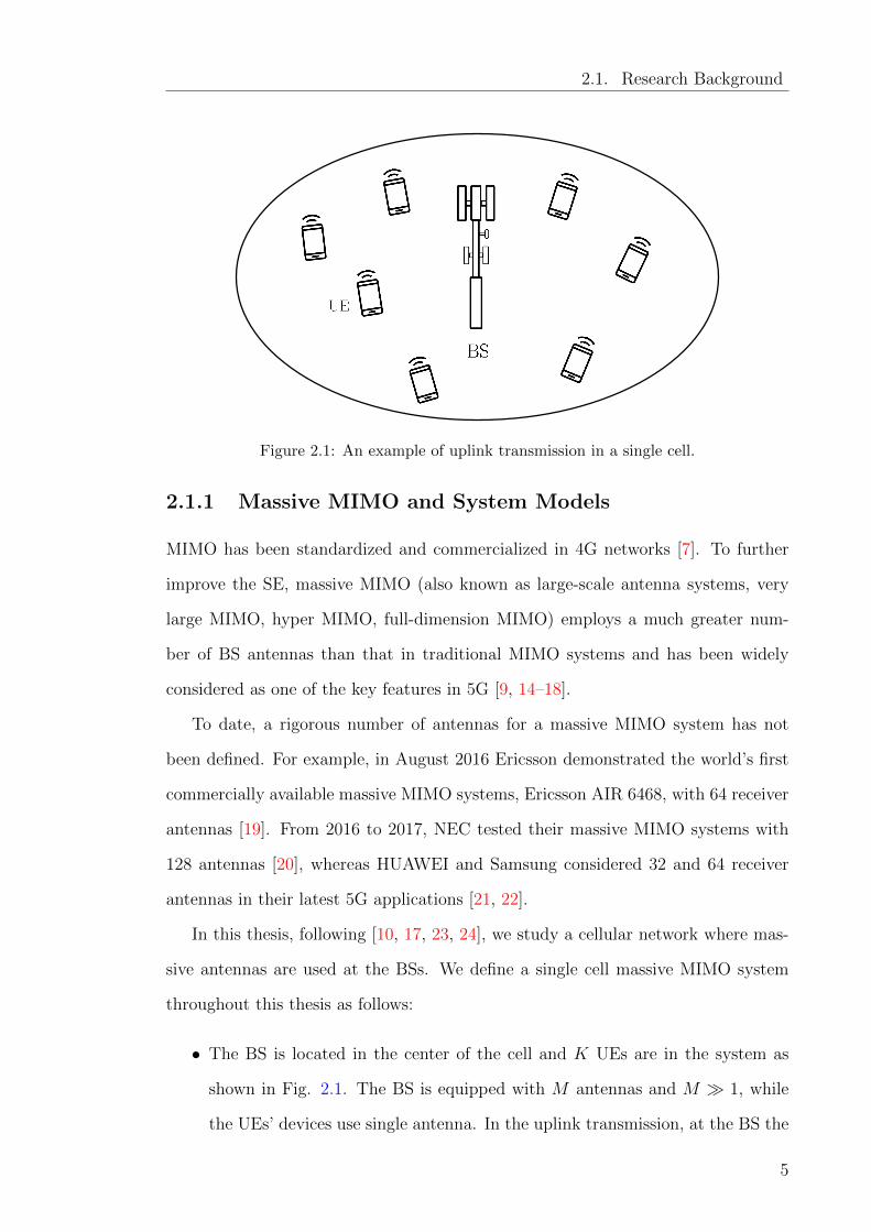
Figure 2.1: An example of uplink transmission in a single cell.
2.1.1 Massive MIMO and System Models
MIMO has been standardized and commercialized in 4G networks [7]. To further
improve the SE, massive MIMO (also known as large-scale antenna systems, very
large MIMO, hyper MIMO, full-dimension MIMO) employs a much greater num-
ber of BS antennas than that in traditional MIMO systems and has been widely
considered as one of the key features in 5G [9, 14–18].
To date, a rigorous number of antennas for a massive MIMO system has not
been defined. For example, in August 2016 Ericsson demonstrated the world’s first
commercially available massive MIMO systems, Ericsson AIR 6468, with 64 receiver
antennas [19]. From 2016 to 2017, NEC tested their massive MIMO systems with
128 antennas [20], whereas HUAWEI and Samsung considered 32 and 64 receiver
antennas in their latest 5G applications [21, 22].
In this thesis, following [10, 17, 23, 24], we study a cellular network where mas-
sive antennas are used at the BSs. We define a single cell massive MIMO system
throughout this thesis as follows:
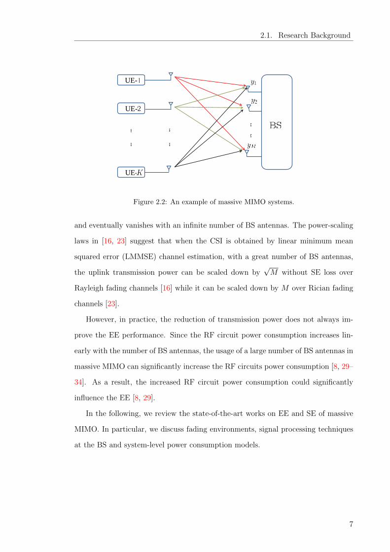
• The BS is located in the center of the cell and K UEs are in the system as
shown in Fig. 2.1. The BS is equipped with M antennas and M 1, while
the UEs’ devices use single antenna. In the uplink transmission, at the BS the
5
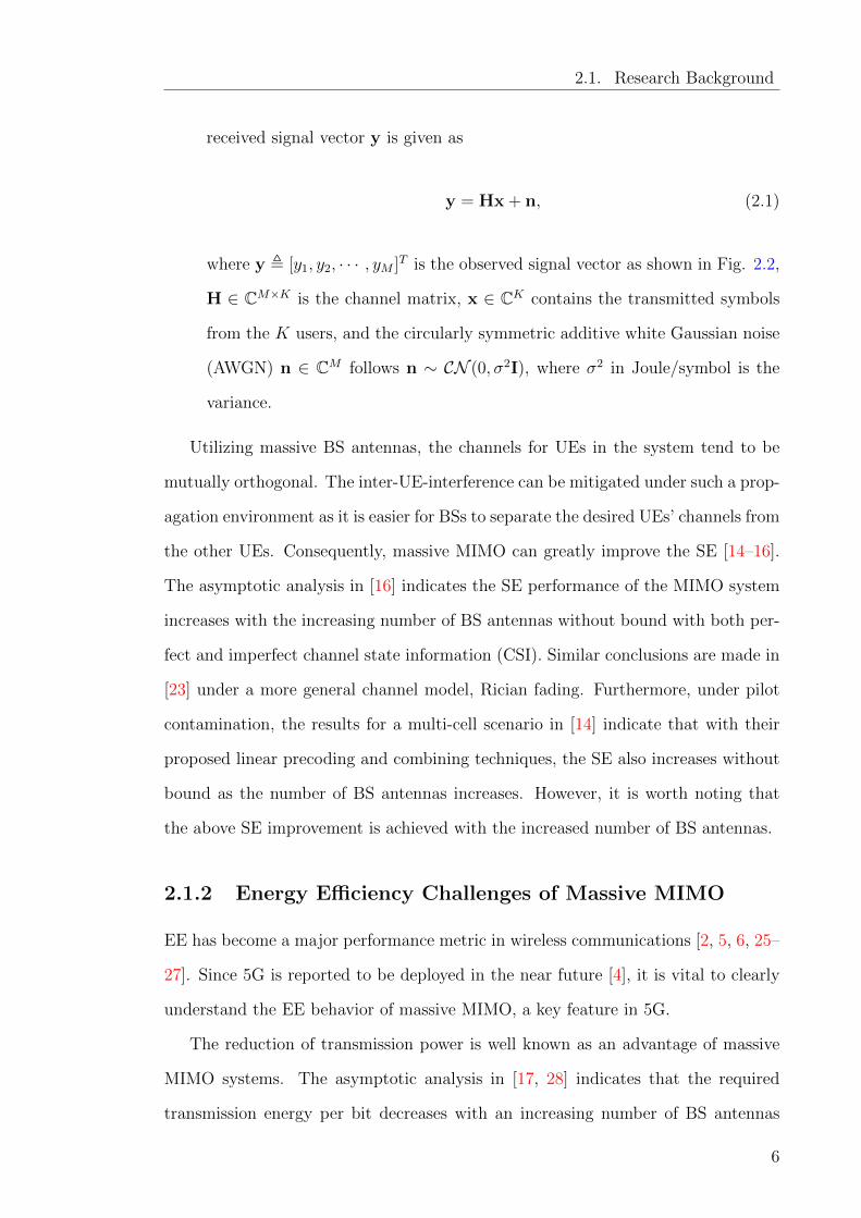
2.1. Research Background
received signal vector y is given as
y = Hx + n, (2.1)
where y , [y1, y2, · · · , yM ]T is the observed signal vector as shown in Fig. 2.2,
H ∈ CM×K is the channel matrix, x ∈ CK contains the transmitted symbols
from the K users, and the circularly symmetric additive white Gaussian noise
(AWGN) n ∈ CM follows n ∼ CN (0, σ2I), where σ2 in Joule/symbol is the
variance.
Utilizing massive BS antennas, the channels for UEs in the system tend to be
mutually orthogonal. The inter-UE-interference can be mitigated under such a prop-
agation environment as it is easier for BSs to separate the desired UEs’ channels from
the other UEs. Consequently, massive MIMO can greatly improve the SE [14–16].
The asymptotic analysis in [16] indicates the SE performance of the MIMO system
increases with the increasing number of BS antennas without bound with both per-
fect and imperfect channel state information (CSI). Similar conclusions are made in
[23] under a more general channel model, Rician fading. Furthermore, under pilot
contamination, the results for a multi-cell scenario in [14] indicate that with their
proposed linear precoding and combining techniques, the SE also increases without
bound as the number of BS antennas increases. However, it is worth noting that
the above SE improvement is achieved with the increased number of BS antennas.
2.1.2 Energy Efficiency Challenges of Massive MIMO
EE has become a major performance metric in wireless communications [2, 5, 6, 25–
27]. Since 5G is reported to be deployed in the near future [4], it is vital to clearly
understand the EE behavior of massive MIMO, a key feature in 5G.
The reduction of transmission power is well known as an advantage of massive
MIMO systems. The asymptotic analysis in [17, 28] indicates that the required
transmission energy per bit decreases with an increasing number of BS antennas
6
2.1. Research Background
UE-
UE-
UE-
Figure 2.2: An example of massive MIMO systems.
and eventually vanishes with an infinite number of BS antennas. The power-scaling
laws in [16, 23] suggest that when the CSI is obtained by linear minimum mean
squared error (LMMSE) channel estimation, with a great number of BS antennas,
the uplink transmission power can be scaled down by√M without SE loss over
Rayleigh fading channels [16] while it can be scaled down by M over Rician fading
channels [23].
However, in practice, the reduction of transmission power does not always im-
prove the EE performance. Since the RF circuit power consumption increases lin-
early with the number of BS antennas, the usage of a large number of BS antennas in
massive MIMO can significantly increase the RF circuits power consumption [8, 29–
34]. As a result, the increased RF circuit power consumption could significantly
influence the EE [8, 29].
In the following, we review the state-of-the-art works on EE and SE of massive
MIMO. In particular, we discuss fading environments, signal processing techniques
at the BS and system-level power consumption models.
7
2.2. Channel Fading
2.2 Channel Fading
In wireless communications, signals are transmitted from transmitters to receivers
over electromagnetic waves. During the transmission, the strength of the signals
may be attenuated by the propagation environment, i.e., a fading channel [35, 36].
In practice, cellular networks are deployed under different environments, e.g., rural
or urban areas. The EE and SE performance of massive MIMO systems can be
different under the various propagation environments [37]. This section provides
the commonly used channel fading models in the performance studies of massive
MIMO systems along with the representative studies on the EE and SE under these
models.
In most massive MIMO studies [1, 10, 23, 24, 38], to characterize the propagation
environments between UEs and the BS, the channel model comprises large-scale and
small-scale fading coefficients. The channel response between UE-k and the m-th
BS antenna can be modeled as
Hmk =√βkHmk, (2.2)
where βk denotes the large-scale fading between UE-k and the BS, while Hmk rep-
resents the small-scale fading between UE-k and the m-th BS antenna. Following
[1, 10, 16, 38], we assume the large-scale fading coefficient, βk, is independent of
the M BS antennas and does not change over coherence blocks. In the following
discussion, we distinguish between large-scale fading models and small-scale fading
models and discuss the state-of-the-art works for both models.
2.2.1 Large-Scale Fading
In general, the large-scale fading models the path loss caused by distances and shad-
owing by objects, such as buildings in the cities. As such, a proper large-scale fading
model is useful for the design of cellular networks, e.g., for the design of cell size
8
2.2. Channel Fading
and density and for the location of BSs in practical deployment [39]. The models
of large-scale fading are widely used to estimate the path loss with the environmen-
tal information, e.g., distances between transmitters and receivers. Assuming the
distance between the transmitter-k and the receiver is dk. The large-scale fading
between the transmitter and receiver is usually characterized (in decibels) as [24, 35]:
Bk = Υ− 10κlog10
(dkd0
)+ Fk dB, (2.3)
where κ denotes the path loss exponent [24] and Υ is the average channel gain
at a reference point, which is d0 far from the receiver. These parameters can be
obtained by practical measurements [40, 41] or approximations based on the carrier
frequency and antennas gain etc.[24]. The shadowing effect models the physical
blockage during the transmission and it is characterized by Fk ∼ N (0, σ2shadow) [24],
where the variance σ2shadow depicts the variations of Fk. It is worth noting that the
value of σ2shadow depends on the transmission scenario [42]. In [10], (2.3) is simplified
to a model which characterizes the path loss as a function of distances. Assuming
users are uniformly distributed in a circular cell with radius dmax. The large-scale
fading coefficient in (2.2) for UE-k is modeled as [10]
βk =d
‖dk‖κ, dmin ≤ dk ≤ dmax, 1 ≤ k ≤ K, (2.4)
where dk is the distance between the k-th UE and the BS, dmin is the minimum
distance and d is used to regulate the channel attenuation at dmin [10].
The prediction of SE performance for a massive MIMO system largely lies in
large-scale fading since the performance become independent of the small-scale fad-
ing when a very large number of BS antennas is employed [17, 43]. For example,
based on the large-scale fading model of the propagation environment, the EE of
massive MIMO systems for a multi-cell scenario is studied in [44, 45], and the BS
density is optimized in homogeneous and heterogeneous cellular networks for maxi-
mal EE [46].
9
2.2. Channel Fading
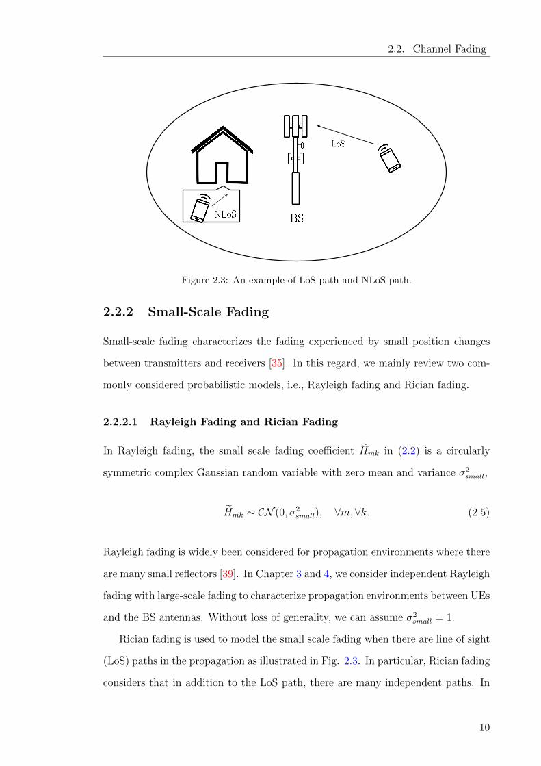
Figure 2.3: An example of LoS path and NLoS path.
2.2.2 Small-Scale Fading
Small-scale fading characterizes the fading experienced by small position changes
between transmitters and receivers [35]. In this regard, we mainly review two com-
monly considered probabilistic models, i.e., Rayleigh fading and Rician fading.
2.2.2.1 Rayleigh Fading and Rician Fading
In Rayleigh fading, the small scale fading coefficient Hmk in (2.2) is a circularly
symmetric complex Gaussian random variable with zero mean and variance σ2small,
Hmk ∼ CN (0, σ2small), ∀m,∀k. (2.5)
Rayleigh fading is widely been considered for propagation environments where there
are many small reflectors [39]. In Chapter 3 and 4, we consider independent Rayleigh
fading with large-scale fading to characterize propagation environments between UEs
and the BS antennas. Without loss of generality, we can assume σ2small = 1.
Rician fading is used to model the small scale fading when there are line of sight
(LoS) paths in the propagation as illustrated in Fig. 2.3. In particular, Rician fading
considers that in addition to the LoS path, there are many independent paths. In
10
2.2. Channel Fading
this case, the small scale fading coefficient Hmk is modeled as a complex Gaussian
random variable with a non-zero mean,
Hmk ∼ CN
(√KkKk + 1
Hmk,1
Kk + 1σ2small
), (2.6)
where Kk is the K-factor for UE-k, which determines the ratio between the power
gains of the LoS component and non-LoS component. For uniform linear array
(ULA), the deterministic LoS component Hmk between UE-k and antenna m can
be characterized by
Hmk = e−j(m−1)(2πd/λ)sin(θk), (2.7)
where d is the antenna spacing, λ is the wavelength and θk is the arrival angle (AoA)
of UE-k.
In Chapter 5, we consider the uplink of a single-cell MIMO system with M BS
antennas and K single-antenna UEs. We consider Rician fading to characterize the
small-scale fading between UEs and BSs. Following [1, 23, 38], we assume a ULA
with half-wavelength spacing, i.e., d = λ/2, where d is the antenna spacing and λ is
the wavelength. The LoS component in (2.7) can be further written as
Hmk = e−j(m−1)π sin(θk) (2.8)
where the AoA θk is uniformly distributed in [−π/2, π/2].
2.2.2.2 Other Fading Models
There are many other small-scale fading models, which may be useful to characterize
certain transmission environments, e.g., Suzuki Model, Nakagami Model, Weibull
Model. This thesis mainly considers Rician fading and Rayleigh fading, while the
details for the rest models can be found in [35].
11
2.2. Channel Fading
2.2.2.3 Channel Hardening and Favorable Propagation
In the study of massive MIMO with a large number of BS antennas, the channel gains
between UEs and BS become nearly deterministic, namely the channel hardening
phenomena [47]. Following [16, 23], channel hardening can be observed in a system
when
‖hk‖2
E[‖hk‖2
] a.s.→ 1, (2.9)
or
1
M|hHk hk| −
1
ME[‖hk‖2
]a.s.→ 0. (2.10)
In practice, under uncorrelated fading, the channel hardening condition can be
satisfied in typical massive MIMO systems [24] and the corresponding asymptotic
analysis leads to high-accuracy performance prediction. With channel hardening,
the EE is independent of the small-scale fading, which largely simplifies the perfor-
mance analysis. The asymptotic analysis yields many vital conclusions on SE and
EE for different scenarios [5, 10, 17, 24, 48]. For example, [5] shows that the EE does
not monotonically increase with SE when transmission power and signal processing
power consumption are both considered. In addition, with a 2D antennas array,
under space-constraint, [49] shows that the EE does not monotonically increase
with the increasing number of antennas due to strong spatial correlation between
the BS antennas. The optimal number of BS antennas, UEs and transmit power
for the maximal EE are investigated in [10] for ZF receivers. Furthermore, differ-
ent channel estimation techniques, e.g., least-square (LS), MMSE and element-wise
MMSE (EW-MMSE) are considered in multi-cell scenarios [50, 51]. The results show
that MMSE estimation leads to the highest SE and the performance gaps between
MMSE and other channel estimations tend to be greater with increasing number of
BS antennas.
In addition to channel hardening, due to the use of massive BS antennas, the
channels for any two UEs in the system tend to be orthogonal, which is known as
12
2.3. Signal Processing
favorable propagation [47]. This leads to the mitigation of the inter-UE-interference
[24]. Generally, this property improves the SE. Following [24], the channel is favor-
able when
hHi hk√E[‖hi‖2
]E[‖hk‖2
] a.s.→ 0 (2.11)
Based on the law of large number, this condition can be satisfied by massive MIMO
when the number of BS antennas is large [16, 23].
The transmission power of massive MIMO can be reduced under favorable prop-
agation [16, 17, 23]. In [17], Thomas indicates the transmit energy vanishes with
an infinite number of antennas at the receiver, even with a low complexity MRC
receiver. This study is then extended to systems with other linear receivers, e.g.,
zero forcing (ZF) [16, 23] and MMSE [16]. In [16], Ngo et al. investigate the SE
performance of massive MIMO with MRC, ZF and LMMSE receivers over Rayleigh
fading. The asymptotic approximations of the SE for both perfect and imperfect
CSI are derived. Utilizing the approximations, the power-scaling laws are derived
for the three linear receivers, which show that the transmission power can be scaled
by the number of BS antennas, i.e., M with perfect CSI and√M when the CSI is
estimated by LMMSE channel estimation. This work is extended to a Rician fading
channel in [23], where the power-scaling laws show that the transmission power can
be scaled by M in Rician fading channels without loss of SE under both perfect and
imperfect CSI.
2.3 Signal Processing
In the uplink, ADCs are used at the BS to convert the received analog signals into
digital signals. A detector is then used to recover the transmitted signals. The
detection usually invokes the knowledge of the channel responses, which can be
acquired by pilot-based channel estimations.
In the remaining of this section, we first review the effect of ADC quantization on
13
2.3. Signal Processing
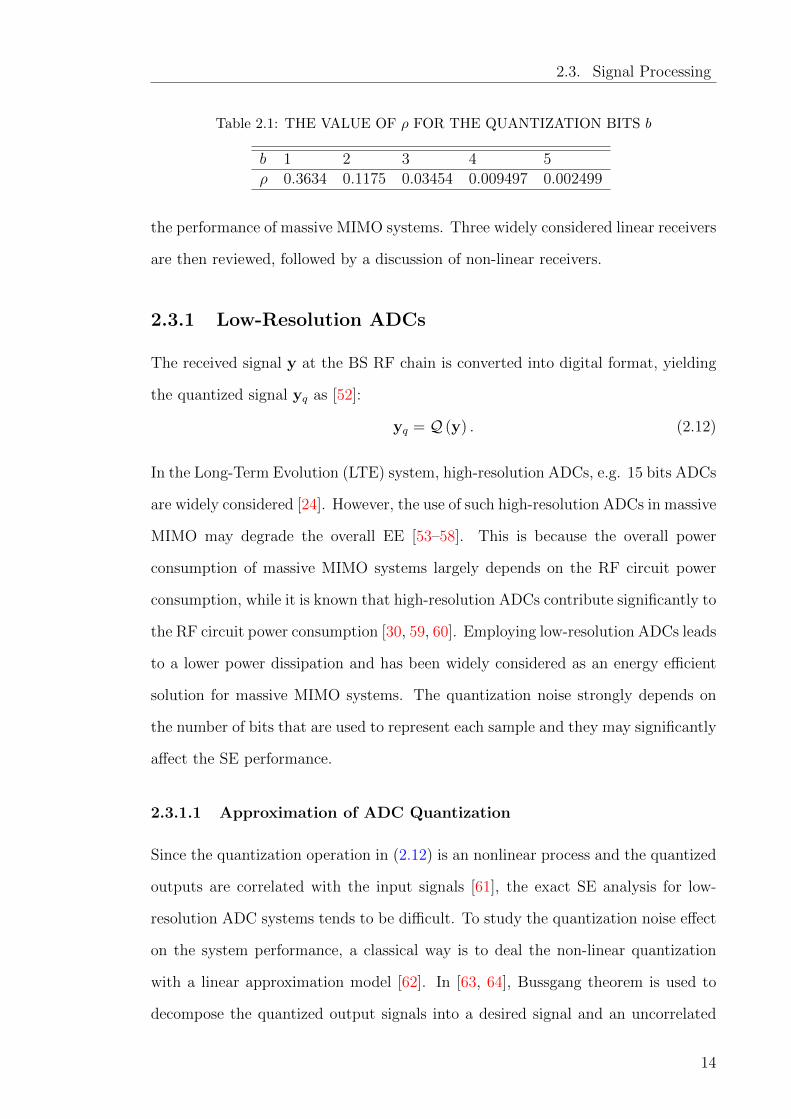
Table 2.1: THE VALUE OF ρ FOR THE QUANTIZATION BITS b
b 1 2 3 4 5ρ 0.3634 0.1175 0.03454 0.009497 0.002499
the performance of massive MIMO systems. Three widely considered linear receivers
are then reviewed, followed by a discussion of non-linear receivers.
2.3.1 Low-Resolution ADCs
The received signal y at the BS RF chain is converted into digital format, yielding
the quantized signal yq as [52]:
yq = Q (y) . (2.12)
In the Long-Term Evolution (LTE) system, high-resolution ADCs, e.g. 15 bits ADCs
are widely considered [24]. However, the use of such high-resolution ADCs in massive
MIMO may degrade the overall EE [53–58]. This is because the overall power
consumption of massive MIMO systems largely depends on the RF circuit power
consumption, while it is known that high-resolution ADCs contribute significantly to
the RF circuit power consumption [30, 59, 60]. Employing low-resolution ADCs leads
to a lower power dissipation and has been widely considered as an energy efficient
solution for massive MIMO systems. The quantization noise strongly depends on
the number of bits that are used to represent each sample and they may significantly
affect the SE performance.
2.3.1.1 Approximation of ADC Quantization
Since the quantization operation in (2.12) is an nonlinear process and the quantized
outputs are correlated with the input signals [61], the exact SE analysis for low-
resolution ADC systems tends to be difficult. To study the quantization noise effect
on the system performance, a classical way is to deal the non-linear quantization
with a linear approximation model [62]. In [63, 64], Bussgang theorem is used to
decompose the quantized output signals into a desired signal and an uncorrelated
14
2.3. Signal Processing
noise.
In this thesis, we invoke additive quantization noise model (AQNM), which is a
linear approximation of the non-linear ADC quantization, to derive the achievable
rate and power allocation for the system. It has been shown [30, 52, 62, 65, 66] that
the AQNM provides an effective and simple approach for analyzing the effects of
ADC quantization noise on the system performance. Although an exact capacity
analysis for massive MIMO with finite-resolution ADCs seems still unknown [67],
AQNM has been widely adopted in many studies to understand the behavior of
low-resolution ADCs and receiver design of low-complexity detectors or system op-
timization. It is reported [68] that AQNM is useful in providing fast performance
estimation compare with other analysis methods. It is worth noting that apply-
ing more sophisticated tools such as generalized mutual information (GMI) [69] to
analyze and optimize the system performance shall be interesting. However, the ca-
pacity analysis, resource allocation, and the corresponding transceiver design could
be more complex.
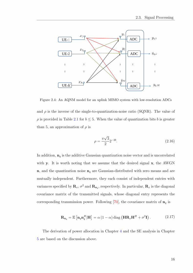
We now introduce AQNM, following [70]. Consider the system model in Section
2.1 and assume equal power for all UEs. At the BS, the received signal y is given as
y =√puHx + n (2.13)
where x is the transmitted unit-power symbols, and pu is the transmission power.
Following [30, 70], we consider a scalar non-uniform quantizer. After quantization,
the output yq , [yq,1, yq,2, · · · , yq,M ] as shown in Fig. 2.4 can be modeled as
yq = αy + nq = α√puHx + αn + nq, (2.14)
where the coefficient α can be obtained by
α = 1− ρ (2.15)
15
2.3. Signal Processing
UE- ADC
UE-
UE-
ADC
ADC
Figure 2.4: An AQNM model for an uplink MIMO system with low-resolution ADCs
and ρ is the inverse of the single-to-quantization-noise ratio (SQNR). The value of
ρ is provided in Table 2.1 for b ≤ 5. When the value of quantization bits b is greater
than 5, an approximation of ρ is
ρ =π√
3
22−2b. (2.16)
In addition, nq is the additive Gaussian quantization noise vector and is uncorrelated
with y. It is worth noting that we assume that the desired signal x, the AWGN
n, and the quantization noise nq are Gaussian-distributed with zero means and are
mutually independent. Furthermore, they each consist of independent entries with
variances specified by Rx, σ2 and Rnq , respectively. In particular, Rx is the diagonal
covariance matrix of the transmitted signals, whose diagonal entry represents the
corresponding transmission power. Following [70], the covariance matrix of nq is
Rnq = E[nqn
Hq |H
]= α (1− α) diag
(HRxH
H + σ2I). (2.17)
The derivation of power allocation in Chapter 4 and the SE analysis in Chapter
5 are based on the discussion above.
16
2.3. Signal Processing
2.3.1.2 The SE and EE of Systems With Low-Resolution ADC
Utilizing AQNM, the analysis in [70] suggests that the loss of the achievable SE
due to the use of low-resolution ADCs can be compensated by employing more BS
antennas. This is further investigated in [71] for imperfect CSI. The results show
that when the numbers of pilot symbols and receiver antennas are large enough, high
SE can still be achieved. The study is then extended to Rician fading [1], where the
more general asymptotic expression of SE is obtained and conclusions similar to [70]
are drawn.
The EE can be improved by jointly optimizing the ADC resolution and the
number of BS antennas [72–74]. This is studied in [75] for MRC receivers using
a system-level power consumption model. The results suggest that ADCs with
moderate resolutions, e.g., 4- or 5-bits ADCs, can optimize the EE, while using
ADCs with extreme low-resolutions, e.g., 1-bit, may degrade the EE since a great
number of BS antennas is required to compensate the SE loss. The analysis is then
extended to the comparison of low-resolution ADCs with mixed ADCs architecture
under Rician fading in [38]. It is shown that the EE can be improved by using low-
resolution ADCs but the mixed-ADC architecture may lead to a better trade-off
between SE and EE.
2.3.2 Linear Signal Detection
After ADC quantization, signal detectors are used to recover the signals. Receiver
signal processing for mitigating the inter-UE-interference significantly influences the
achievable SE and EE of massive MIMO systems.
In this part, we first review three widely considered linear receivers: MRC, ZF
and MMSE receivers. Under linear signal detection, each of the transmitted data
streams x are estimated at the receivers as a linear transformation of the observed
signals y [76]. Let the linear receiver for theK UEs be G = [g1,g2, . . . ,gK ] ∈ CM×K .
17
2.3. Signal Processing
The estimated signals are given as
x = GHy (2.18)
where G is the linear weight matrix to be designed. Specifically, the weight matrices
for the three detection are given as
G =
H, MRC
H(HHH)−1, ZF
(HPHH + σ2IM)−1HP, LMMSE
(2.19)
where P is a diagonal matrix with the transmitted of power of the UEs on its
diagonal.
In signal processing, MRC is known as low complexity receiver as it does not
involve any matrix inversion. For ZF receivers, if the system satisfies M > K, the
weight matrix is given as the pseudo-inverse of the channel matrix as shown in (2.19).
Ideally, ZF enables multiple antenna receivers to null the multi-UEs’ interference,
i.e.,
x = x + GHn. (2.20)
It is noted that the noise can be enhanced [76] by ZF receivers from (2.20). According
to [76], MMSE receivers are able to address the drawback of noise enhancement
by considering MMSE criterion. Specifically, it minimizes the mean square error
between the transmitted signals and the recovered signals, i.e., minE‖x− x‖2.
Generally, ZF outperforms MRC in the SE performance at high signal-to-noise ratio
(SNR). The SE gap between ZF and MMSE is narrowed down when the SNR is
high, as the noise enhancement with ZF receivers is alleviated.
The achievable SE of massive MIMO systems with linear receivers has been
studied in many works. Assuming ideal ADCs, [16, 17] suggest high SE performance
can be achieved with linear receivers, such as MRC, ZF or MMSE receivers since the
intra-cell interference can be suppressed with a very large number of BS antennas.
18
2.3. Signal Processing
Generally, the SE performance of MMSE outperforms MRC and ZF receivers, while
ZF performs better than MRC receivers at high SNR [16] with the same number of
antennas. The SE gap between MRC and the other two receivers can be mitigated
with additional number of antennas and strong LoS paths. The additional number
of antennas for MRC receiver to achieve the same SE performance of MMSE is
studied in [48]. The fact that increasing the value of Rician K-factor can narrow
down the SE gap between MRC and ZF receivers is investigated in [23].
The achievable SE of systems with low-resolution ADCs and linear receivers has
been studied in [38, 70, 77–79]. The results in [70] show that SE comparable to that
with idea ADCs can be achieved with low-resolution ADCs and MRC receivers. In
[77], the SE performance with low-resolution ADCs and MRC and ZF receivers is
investigated, which shows that the ZF receiver outperforms the MRC receiver in
SE when the resolution of ADCs, the numbers of UEs and BS antennas are fixed.
These receivers are also studied in [79] for discrete-valued and Gaussian signaling
using mutual information and AQNM, assuming practical channel estimation. The
achievable uplink SE with the LMMSE receiver is analyzed in [78] for receivers
with 3-bits ADCs, showing that performance close to that with ideal ADCs can be
achieved provided that enough antennas are used at the BS.
Given a receiver, the EE-SE trade-off can be studied with a system level power
consumption model [80]. Assuming a target SE for all UEs, the number of antennas
has been optimized to achieve the maximum EE for MRC, ZF and MMSE receivers
in [10]. The numerical results show that the maximum EE values of MMSE and
ZF are similar but much greater than that with MRC receivers. To achieve the
maximal SE or EE, the optimal number of UEs depends on the linear receivers,
e.g., MRC requiring a larger number of UEs than that with ZF [10, 81]. Under
pilot contamination the EE-SE trade off is studied in [82]. The results suggest when
pilot length equals to half of the coherent block length, the optimal pilot to data
power ration for the maximum SE or EE is 1 [82]. Besides, the EE under a space
constrained rectangular array has been studied with MRC and ZF receivers [49].
19
2.3. Signal Processing
The results indicate the number of antennas for ZF to achieve the maximum EE is
greater than that with MRC receivers and the EE for ZF is higher than that with
MRC receivers.
Generally, the high SE performance can be achieved by linear receivers with the
advantages of favorable propagation [17, 24] in massive MIMO systems. However,
according to the discussion in Section 2.2.2.3, the condition of favorable propagation
is satisfied with a great number of BS antennas. In the EE study, such a large
number of antennas raise a serious concern in terms of the excessive RF chain power
consumption.
2.3.3 Non-Linear SIC Signal Detection
The aforementioned studies on the EE of massive MIMO focus on linear receivers.
By providing more advanced interference cancellation, nonlinear receivers can dra-
matically improve the SE [83], which is able to reduce the number of antennas
requirement of the system with linear receivers to maintain the QoS. As a result,
using nonlinear receivers could mitigate the RF circuit power consumption. How-
ever, it is worth noting that nonlinear receivers usually increase signal processing
energy consumption compared with linear receivers. To date, the trade-offs between
the achievable SE and EE for non-linear receivers have rarely been studied.
Nonlinear receivers such as those based on SIC [39, 84–87] have been intensively
studied for decades. Unlike the linear receivers, SIC receivers are based on inter-
ference cancellation techniques, which are nonlinear process. Specifically, according
to [76, 88, 89], the inter-UE-interference from previous layers are removed before
detecting the current layer’s signal. The signal of UE-k is estimated as
xk = gHk yk, (2.21)
where yk is obtained by canceling the detected signals from the observed signals y
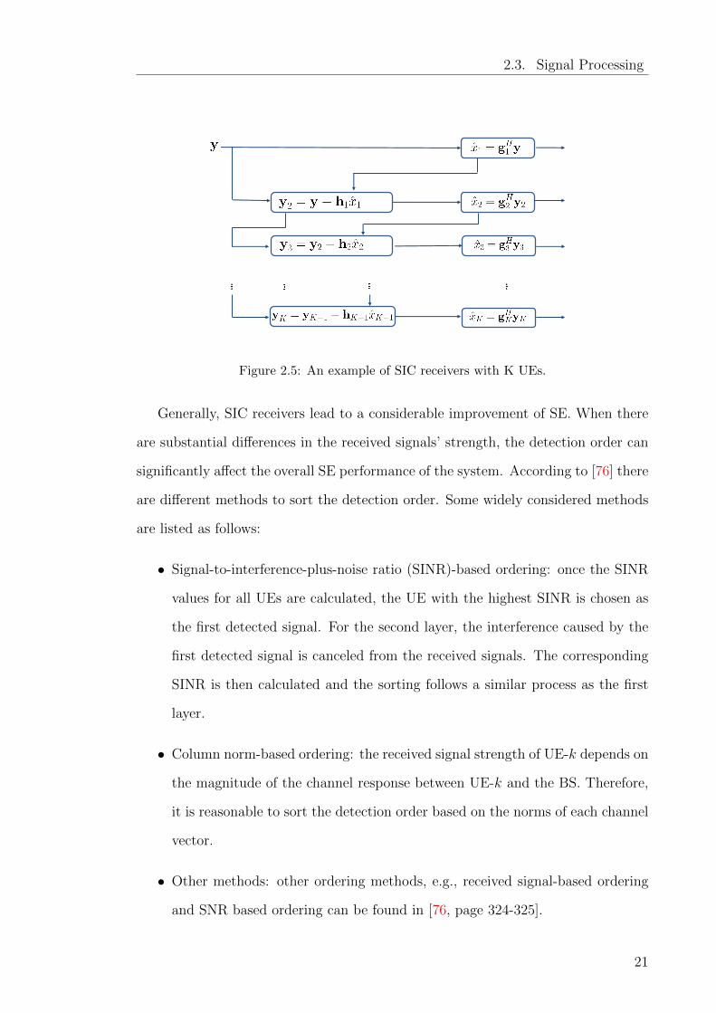
and gk is the corresponding filter. This process is illustrated in Fig. 2.5.
20
2.3. Signal Processing
Figure 2.5: An example of SIC receivers with K UEs.
Generally, SIC receivers lead to a considerable improvement of SE. When there
are substantial differences in the received signals’ strength, the detection order can
significantly affect the overall SE performance of the system. According to [76] there
are different methods to sort the detection order. Some widely considered methods
are listed as follows:
• Signal-to-interference-plus-noise ratio (SINR)-based ordering: once the SINR
values for all UEs are calculated, the UE with the highest SINR is chosen as
the first detected signal. For the second layer, the interference caused by the
first detected signal is canceled from the received signals. The corresponding
SINR is then calculated and the sorting follows a similar process as the first
layer.
• Column norm-based ordering: the received signal strength of UE-k depends on
the magnitude of the channel response between UE-k and the BS. Therefore,
it is reasonable to sort the detection order based on the norms of each channel
vector.
• Other methods: other ordering methods, e.g., received signal-based ordering
and SNR based ordering can be found in [76, page 324-325].
21
2.4. Power Consumption Model
According to [76], the first ordering method involves rather complex computation
of the SINR for obtaining the detection order. By contrast, with the norm-based
ordering method, we only need to calculate the norm of each channel column and
sort them once. Consequently, the ordering complexity can be significantly reduced
with the norm-based ordering.
2.3.3.1 Detection Computational Complexity
For the linear and SIC receivers considered in this part, the signal detection com-
plexity consists of two parts: the first part is for computing the receiver weights
as shown in (2.19) for linear receivers, which is assumed to be done only once for
one coherent block. The second is for applying the receiver weights to each instan-
taneous symbol as illustrated in (2.18). We assume that the receiver weights are
stored and reused. When the coherent block is large, the overall complexity is indeed
dominated by the second part.
2.4 Power Consumption Model
From (1.1), a system-level power consumption model is of paramount importance in
the EE evaluation. Many power consumption models have been proposed to evaluate
and optimize the EE performance of cellular networks from different aspects [90–93].
For example, with the power model in [90], the EE performance of a single-input
single-output (SISO) system is evaluated and has been improved by optimizing
the modulation and transmission time. A power consumption model for multi-
user code division multiple access (CDMA) systems is then presented in [91] to
study the energy consumption of the system. The power consumed by the analog
signal processing along with the low-density parity-check (LDPC) channel decoder
is modeled in [92]. To study the EE of BSs in LTE systems, a power consumption
model of BSs is developed in [93]. Note that, however, the aforementioned power
consumption models are not proposed for massive MIMO systems. Owing to a great
22
2.4. Power Consumption Model
number of BS antennas, the power consumption model for massive MIMO systems
should be carefully developed.
In massive MIMO systems, the total power consumption arises from the trans-
mission (PTX), the circuits (Pcircuits), i.e.,
Ptotal = PTX + Pcircuits. (2.22)
In [10], Bjornson et al. propose a system level power consumption model for uplink
and downlink massive MIMO systems. Specifically, this model includes every part
from UE handsets to BSs of a MIMO system and the power consumption of detection
is taken into account. This thesis focuses on uplink transmission. Modifying this
model to an uplink transmission scenario allows us to explicitly show the trade-off
between EE and signal processing schemes, e.g., different detection schemes and
low-resolution ADC systems in an uplink transmission.
We next show the modified power consumption model of uplink massive MIMO
systems and this model is considered in Chapter 3, 4 and 5.
2.4.1 A System-Level Power Consumption Model for Up-
link Transmission
The modified model is used to evaluate the power consumption of the uplink single-
cell MIMO system as introduced in Section 2.1.1. The system operates in a time-
division duplex (TDD) mode with a bandwidth of B Hz and the BS and UEs are
perfectly synchronized. We assume that U symbols are transmitted in total for the
uplink and downlink within a time-frequency coherence block. Let the uplink ratio
be ζul. Then Uζul symbols are transmitted in the uplink. We further assume that
τulK out of the Uζul uplink transmission symbols are used for channel estimation,
where τul specifies the pilot length. In the following part, the total power consump-
tion is analyzed and falls into two parts, which are: signal transmission part and
circuit part.
23
2.4. Power Consumption Model
1. Signal transmission part : The average uplink signal transmit power, PTX, is
defined as the power consumed by power amplifiers in an uplink transmission
and this contains the dissipation and transmit power. If we assume the power
amplifier efficiency η to be the same for each UE, according to [10] we then
have:
PTX =Bζul
ηE1TKp Watt. (2.23)
As mentioned in [10], a uniform gross rate R is assigned to each UE in order
to address disparity between peak and average rates. This can be achieved
by proper power allocation e.g. p = [p1, p2, . . . pK ]T and the details of power
allocation are provided in Chapter 3 and 4 under their corresponding assump-
tions.
2. Circuit part : The circuit power consumption accounts for the analog and
digital signal processing power consumption and the power consumption of
other components. According to [10], the analog part at both transmitters
and receivers can be described as
PTC = MPBS +KPUE + PSYN Watt, (2.24)
The power contributed by analog signal processing PTC accounts for the power
consumption of the RF circuit components at the BS and UEs. Specifically, all
the power consumption of one RF circuit at the BS is denoted by PBS whereas
PUE is the RF circuit power consumption for each UE. Besides, PSYN is the
power required by local oscillator.
The digital signal processing part includes channel estimation, coding, de-
coding and signal detection. Specifically, the power consumption of LMMSE
channel estimation is modeled as:
PCE =B
U
2τMK2
LBS
Watt, (2.25)
24
2.4. Power Consumption Model
where LBS denotes the computational efficiency at the BS in flops/Watt. The
power consumption of channel coding and decoding is modeled as:
PCD =K∑k=1
ERk (PCOD + PCED) Watt, (2.26)
where the channel coding and decoding powers are denoted by PCOD and
PCED respectively. Finally, the power consumption of signal detection part is
modeled as follow:
PSD = Bζul(
1− Kτ
ζulU
)Csymbol
LBS
+ PWM Watt, (2.27)
where Csymbol denotes the complexity for the detection of the K users’ signal for
each information-carrying symbol, e.g., following [10] Csymbol = 2KM for ZF
and MRC receivers and PWM is the power consumed by the detection weight
matrix computation and depends on the complexity for finding the weight
matrix. For example, considering MRC, following [10]:
P(MRT/MRC)WM =
B
U
C(MRT/MRC)w
LBS
Watt, (2.28)
where C(MRT/MRC)w = 3MK is the complexity for finding the weight matrix of
MRC receivers.
The other components power consumption can be modeled by a load-independent
part and a load-dependent part:
Pothers = PFIX +∑K
k=1ERkPBT Watt, (2.29)
where the load-independent term PFIX is the power consumption used to site
cooling, control signaling, and base band processors while the load-dependent
PBT counts for the power of backhaul and control signal in Watt per bit/s.
25
2.4. Power Consumption Model
2.4.2 Low-Resolution ADC Power Consumption
As shown in (2.24), there is a considerable increase in the total RF circuit power
consumption, i.e., MPBS, when the number of antennas, M , is large. For example,
following [93], the power consumption of RF circuit will be more than 160 Watts
for a BS with 200 antennas, while the total power consumption for a traditional BS
with 2 antennas is in a range from 60 Watts to 150 Watts [93]. As explained earlier
in Section 2.3.1, the use of low-resolution ADCs at the RF chains has been widely
considered as a promising solution to address the power consumption issue. The
power consumption models for low-resolution ADCs are reviewed in this part and
used in Chapter 4 and 5 to evaluate the EE of massive MIMO systems with low-
resolution ADCs. According to [59], analog to digital conversion includes two main
operations, sampling and quantization. The ADCs power consumption is mainly
determined by its sampling rate and resolution bits [30, 94]. The overall power
consumption of ADCs can be modeled by [30]
PADC = FOM · fsampling · 2b Watt, (2.30)
where fsampling stands for the sampling rate and the figure of merit (FOM) means
energy consumed per conversion step.
2.4.2.1 Sampling Rate
Nyquist rate is the minimum sampling rate to avoid aliasing and is considered in
this thesis. Meanwhile, in analog to digital conversion, oversampling uses a sampling
rate which is greater than the Nyquist rate and this is quite often a case in the ADC
design [59],[95, 96]. In [59, 95–98], the advantages provided by oversampling refer to
process gain, which can increase the SNR at baseband. The SNR can be increased
by 20 to 40 dB [95]. On the other hand, it is noted that oversampling leads to some
disadvantages, e.g., excessive power consumption and setup time issues.
26
2.5. Motivations
2.4.2.2 Resolution
In analog to digital conversion, the number of quantization levels depends on the
resolution of the ADCs [59]. For example, 3-bits ADCs can provide 8 different levels
for the quantization output signals. Generally, an ADC with high resolution leads
to smaller quantization error compared with a low-resolution ADC. However, this
is accompanied by higher circuit power consumption, as shown in (2.30).
2.4.2.3 FOM
It is reported in [99] that the FOM is improved by a factor of 1.8 for each new gener-
ation of complementary metal-oxide-semiconductor (CMOS) technology. According
to the recently works in [100], it is clear that the performance of FOM has been
improved in the last decades. Since most ADCs reported in the recently published
paper have not been commercialized yet, in Chapter 4 and 5, to evaluate EE perfor-
mance of a massive MIMO system with low-resolution ADCs, we choose a moderate
reference value from [100], 1432.1 (fJ/conv-step).
2.5 Motivations
The previous part of this chapter reviews the state-of-the-art works on the SE and EE
of massive MIMO. The EE performance of massive MIMO systems strongly depends
on the receivers and RF hardware design. Previous studies have put many efforts
to gain a thorough understanding of how receiver design and imperfect hardware
influence the EE. However, these works still have limitations in certain aspects as
follows:
• Receiver design: The EE performance of massive MIMO systems is largely
affected by the receiver design, as the number of antennas needed to achieve
a given quality of service (QoS) depends on the receiver architecture. The EE
study of massive MIMO systems to date has focused on linear receivers. It is
27
2.5. Motivations
found [101] that applying a more sophisticated linear receiver may reduce the
number of BSs antennas needed, which results in lower power consumption of
RF circuits and hence improve the overall EE. On the other hand, nonlinear
receivers such as those based on SIC [39, 85–87] and iterative processing [102–
104] have been intensively studied for cellular communications. It is shown
that the SE performance can be substantially improved by providing more
sophisticated interference cancellation, using nonlinear receivers. However,
this is often accompanied by increased energy consumption of receiver signal
processing. The trade-off between the achievable SE and EE has been less
understood for nonlinear receivers as compared to the more widely studied
linear receivers.
• Low-resolution ADCs: It has been known that [105] a major part of the
RF circuit power is consumed by the high-resolution ADCs. Although high-
resolution ADCs introduce less quantization errors, their exponentially in-
creasing power dissipation can degrade the overall EE [59, 60]. The feasibility
of massive MIMO systems with low-resolution ADCs in practical cellular net-
works has been studied in [1, 38, 67, 70, 71, 77, 78, 106]. The results suggest
with a great number of antennas, SE comparable to that with idea ADCs can
be achieved with low-resolution ADCs. The EE can be improved by jointly
optimizing the ADC resolution and the number of BS antennas [72–74]. This
is studied in [75] for maximal ratio combining (MRC) receivers using a system-
level power consumption model. The results suggest that ADCs with moderate
resolutions can optimize the EE, while using ADCs with too low resolutions
may degrade the EE due to the rapid increase of the number of BS anten-
nas required. The current works focus on a single cell system and use a great
number of antennas to compensate the SE loss due to the use of low-resolution
ADCs. Whether the EE can be further improved by a sophisticated receiver
is unknown, while the EE analysis of the system for multi-cell is missing in
28
2.6. Summary
the current literature.
• Channel fading: As commercial cellular networks are deployed under various
propagation environments, the corresponding EE behavior and performance
should be carefully studied and evaluated under a proper fading model [37].
For applications such as small-cell networks [107], wireless-powered-Internet of
things (WP-IoT) [108] and unmanned aerial vehicles (UAV) to ground trans-
missions [109], it is reasonable to model the channels as Rician fading chan-
nels, which consider line-of-sight (LoS) paths between the transmitters and
receivers. The SE performance and power scaling of massive MIMO systems
over Rician fading channels have been studied in [23] under both perfect and
imperfect CSI. This work is then extended to the systems with low-resolution
ADCs [1] and the mixed-ADC systems [38]. However, in the aforementioned
works [1, 38], the CSI is assumed to be estimated using a small number of
ideal ADCs with a round-robin process. It has been demonstrated in [110]
that the training time can be significantly reduced when all the BS antennas
are actively linked to ADCs at any time over Rayleigh fading channels, while
there is a paucity of studies on the performance over Rician fading channels.
2.6 Summary
In light of the above discussions, in the next three chapters we focus on the EE
and SE evaluations of massive MIMO systems with SIC receivers and low-resolution
ADCs under different fading environments.
29
Chapter 3
Energy Efficiency of Uplink Massive
MIMO Systems With Successive
Interference Cancellation
3.1 Introduction
In this chapter, we study the uplink EE achievable when SIC based nonlinear re-
ceivers are applied, in contrast to the previous studies focusing only on linear re-
ceivers. Zero forcing (ZF)-SIC and minimum mean squared error SIC (MMSE-SIC)
[88] are investigated and an asymptotic analysis of the total transmission power is
provided for ZF-SIC receivers. We show that employing SIC receivers can notice-
ably reduce the number of needed BS antennas compared to linear receivers for
given transmission rates. Meanwhile, the complexity of a SIC receiver can be kept
comparable with the classical linear receivers. Consequently, the overall EE can be
improved by employing the SIC receivers.
We organize the rest of this chapter as follows. In Section 3.2, we discuss the
30
3.2. System Model and EE With a Linear Receiver
system model and review the EE analysis for massive MIMO systems with linear
receivers. We analyze the EE with SIC based receivers in Section 3.3, and present
simulation results in Section 3.4. We summarize this chapter in Section 3.5.
3.2 System Model and EE With a Linear Receiver
3.2.1 System Model
In this chapter we consider an uplink single-cell MIMO system as defined in Section
2.1.1. Recall that the signal model is given by
y = Hx + n, (3.1)
where y ∈ CM is the observed signal vector at the BS, H ∈ CM×K is the channel
matrix, x ∈ CK contains the transmitted symbols from the K users, and n ∈ CM is
the AWGN with variance σ2 (in Joule/symbol).
Let Hm,k be the (m, k)-th entry of H, denoting the channel gain between the
k-th UE and the m-th BS antenna. As defined in (2.2), we assume a channel model
with Hmk =√βkHmk, where βk, defined in (2.4), represents the path loss between
UE-k and the BS, while Hmk characterizes independent Rayleigh fading between the
k-th UE and the m-th BS antenna. We can write
H = Hdiag(√β1,√β2. · · · ,
√βK), (3.2)
where H is the Rayleigh fading component of H.
3.2.2 Power Consumption Model
In this chapter, we assume that the system operates in a TDD mode as introduced
in Section 2.4.1 and extend the system-level power consumption model in Section
2.4 to other receivers in order to investigate the trade-off between EE and SE for
31
3.2. System Model and EE With a Linear Receiver
linear and SIC receivers. Following (2.22), the total power consumption is written
as Ptotal = PTX + Pcircuits.
As introduced in (2.23), the power consumed by the power amplifiers at the UEs
in uplink transmission is denoted by PTX. Specifically, PTX can be calculated by the
power amplifier efficiency, η, the bandwidth, B, and p the transmitted power from
the K UEs in Joule/symbol,
PTX =Bζul
ηE1TKp, (3.3)
where 1K is a K dimensional unit vector and p can be calculated by (3.6), (3.11)
and (3.14), respectively, for the linear and SIC receivers.
In this chapter, Pcircuits consists of the circuit power consumptions at BS and
UEs. Specifically, according to [10], Pcircuits ,MPBS +KPUE +PSYN +PCE +PCD +
Pothers + PSD. PBS and PUE denote the power consumption per RF circuit at the
BS and UE, respectively. PCD is consumed by channel coding/decoding in uplink
transmission. PSYN is required by local oscillator at the BS and Pothers denotes the
backhaul power consumption and the power of site cooling, etc. PSD depends on the
complexity of signal detection and will be detailed. The uplink channel estimation
power consumption, PCE, is modified from [10] by ignoring the downlink part.
In this chapter, we investigate the influence of the BS receiver on PTX, Pcircuits
and EE. Before detailing the results with nonlinear receivers in Section 3.3, we first
review the analysis for linear receivers. We assume that perfect uplink CSI is known
at BSs. Following (2.19), the receiver weight matrix of the ZF and LMMSE receivers
are given by
G =
H(HHH)−1, ZF
(HPHH + σ2IM)−1HP, LMMSE(3.4)
where P = diag(p1, p2, . . . , pK) is the diagonal matrix with the power of transmitted
signals from theK UEs on its diagonal. The resulting filter output, i.e. the estimated
transmitted symbol, is: x = GHy. The achievable uplink transmission rate of the
32

3.3. EE With SIC Receivers
k-th user is described as [10]
Rk = ζul(
1− τul K
Uζul
)Rk, (3.5)
where the term 1 − τul KUζul
characterizes the decrease of effective transmission rate
due to the overheard of training, and Rk = R, k = 1, 2, · · · , K, are the same gross
rates of the K UEs. Let gk and hk be the k-th columns of G and H, respectively.
The optimal power allocation for achieving Rk = R, k = 1, 2, · · · , K, satisfies [10]
p = σ2D−11K , (3.6)
where
Dk,l =
|gHk hk|2
(2R/B−1)‖gk‖2, k = l,
− |gHk hl|2‖gk‖2
, k 6= l.
(3.7)
The power consumption of signal detection, including the power PWM for computing
the weight matrix G, is evaluated as
PSD = Bζul(
1− Kτul
ζulU
)2KM
LBS
+ PWM, (3.8)
where LBS denotes the computational efficiency [10]. For the ZF receiver [10],
PWMZF= B
U
(K3
3LBS+ 3MK2+MK
LBS
). For an LMMSE receiver [10], PWMLMMSE
≈ 3PWMZF.
3.3 EE With SIC Receivers
We now analyze the EE when the SIC receivers are employed at the BS. The power
consumptions of the transmitters and signal detection are now different, as analyzed
below.
33
3.3. EE With SIC Receivers
3.3.1 Transmitter Power Consumption
When SIC is used to decode the K UEs’ signals, the signals from already decoded
UEs are assumed ideally canceled. We assume that at the k-th decoding stage, user
1 to k − 1’s signals are already decoded and canceled. With ZF-SIC, the detector
for user k is given by
gk =[Hk(H
Hk Hk)
−1]
:,1, (3.9)
where Hk denotes a matrix formed by the last K − k + 1 columns of H and [·]:,1
means taking the first column of a matrix. It can be verified that gHk hk = 1,∀k,
while gHk hl = 0,∀l > k. Under the assumption of ideal interference cancellation, the
k-th UE’s achievable rate is
Rk = B log
(1 +
pkσ2‖gk‖2
). (3.10)
Assuming Rk = R, ∀k, the corresponding transmit power should be allocated as
pk = (2R/B − 1)σ2‖gk‖2. (3.11)
With the MMSE-SIC receiver, the signals from the remaining UEs are treated as
noise. Assuming ideal interference cancellation, the kth UE’s detector is given by
gk = pk
(K∑j=k
pjhjhHj + σ2IM
)−1
hk. (3.12)
The achievable rate is
Rk = B log
1 + pkhHk
(K∑
j=k+1
pjhjhHj + σ2IM
)−1
hk
, (3.13)
34
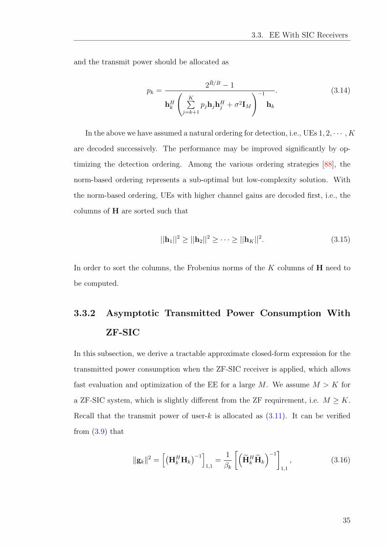
3.3. EE With SIC Receivers
and the transmit power should be allocated as
pk =2R/B − 1
hHk
(K∑
j=k+1
pjhjhHj + σ2IM
)−1
hk
. (3.14)
In the above we have assumed a natural ordering for detection, i.e., UEs 1, 2, · · · , K
are decoded successively. The performance may be improved significantly by op-
timizing the detection ordering. Among the various ordering strategies [88], the
norm-based ordering represents a sub-optimal but low-complexity solution. With
the norm-based ordering, UEs with higher channel gains are decoded first, i.e., the
columns of H are sorted such that
||h1||2 ≥ ||h2||2 ≥ · · · ≥ ||hK ||2. (3.15)
In order to sort the columns, the Frobenius norms of the K columns of H need to
be computed.
3.3.2 Asymptotic Transmitted Power Consumption With
ZF-SIC
In this subsection, we derive a tractable approximate closed-form expression for the
transmitted power consumption when the ZF-SIC receiver is applied, which allows
fast evaluation and optimization of the EE for a large M . We assume M > K for
a ZF-SIC system, which is slightly different from the ZF requirement, i.e. M ≥ K.
Recall that the transmit power of user-k is allocated as (3.11). It can be verified
from (3.9) that
‖gk‖2 =[(
HHk Hk
)−1]
1,1=
1
βk
[(HHk Hk
)−1]
1,1
, (3.16)
35
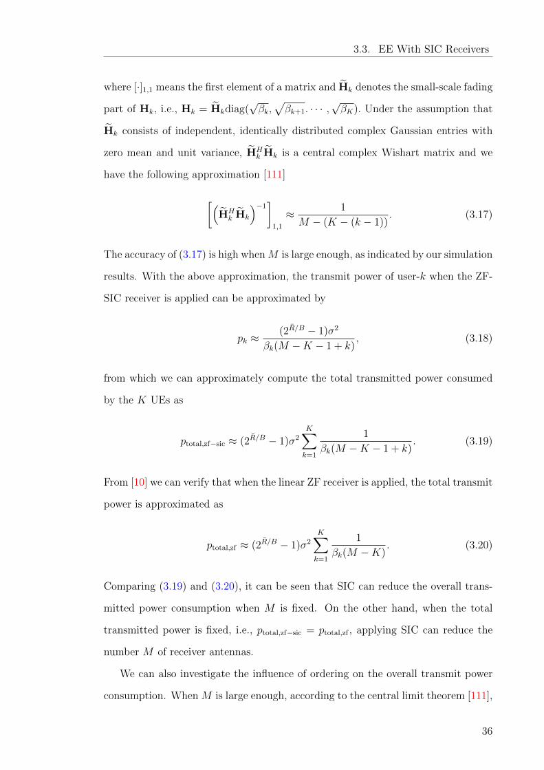
3.3. EE With SIC Receivers
where [·]1,1 means the first element of a matrix and Hk denotes the small-scale fading
part of Hk, i.e., Hk = Hkdiag(√βk,√βk+1. · · · ,
√βK). Under the assumption that
Hk consists of independent, identically distributed complex Gaussian entries with
zero mean and unit variance, HHk Hk is a central complex Wishart matrix and we
have the following approximation [111]
[(HHk Hk
)−1]
1,1
≈ 1
M − (K − (k − 1)). (3.17)
The accuracy of (3.17) is high whenM is large enough, as indicated by our simulation
results. With the above approximation, the transmit power of user-k when the ZF-
SIC receiver is applied can be approximated by
pk ≈(2R/B − 1)σ2
βk(M −K − 1 + k), (3.18)
from which we can approximately compute the total transmitted power consumed
by the K UEs as
ptotal,zf−sic ≈ (2R/B − 1)σ2
K∑k=1
1
βk(M −K − 1 + k). (3.19)
From [10] we can verify that when the linear ZF receiver is applied, the total transmit
power is approximated as
ptotal,zf ≈ (2R/B − 1)σ2
K∑k=1
1
βk(M −K). (3.20)
Comparing (3.19) and (3.20), it can be seen that SIC can reduce the overall trans-
mitted power consumption when M is fixed. On the other hand, when the total
transmitted power is fixed, i.e., ptotal,zf−sic = ptotal,zf , applying SIC can reduce the
number M of receiver antennas.
We can also investigate the influence of ordering on the overall transmit power
consumption. When M is large enough, according to the central limit theorem [111],
36
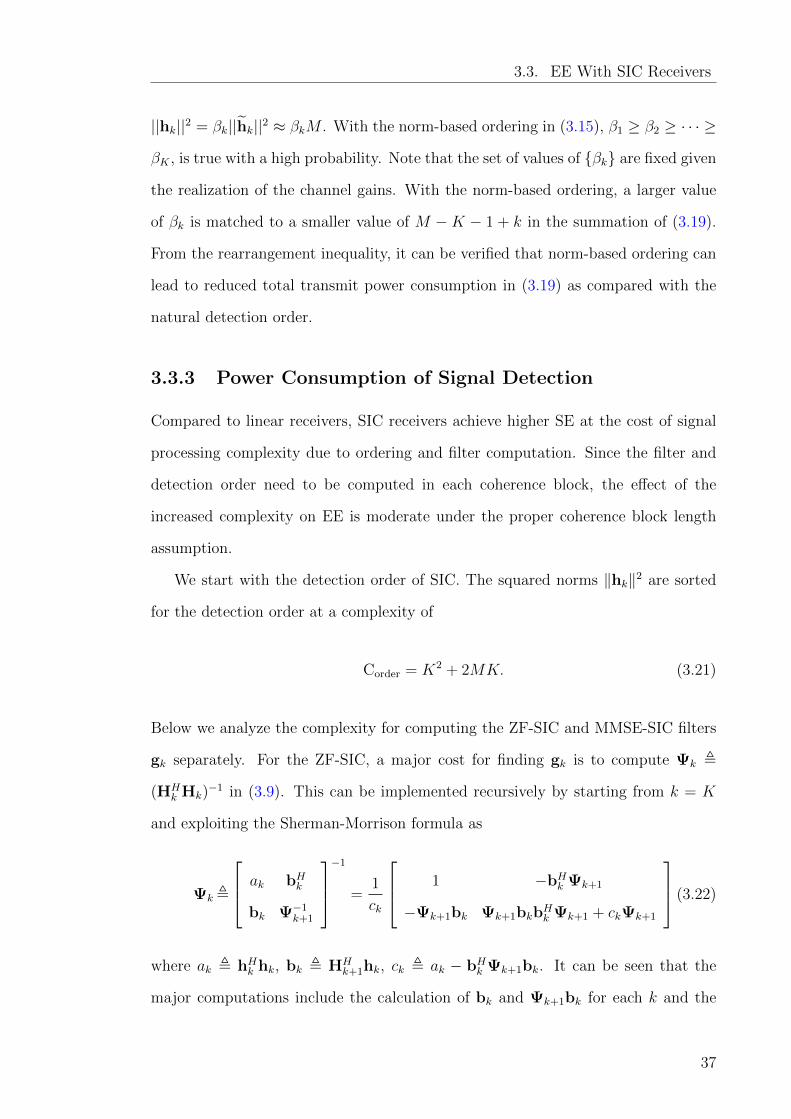
3.3. EE With SIC Receivers
||hk||2 = βk||hk||2 ≈ βkM . With the norm-based ordering in (3.15), β1 ≥ β2 ≥ · · · ≥
βK , is true with a high probability. Note that the set of values of βk are fixed given
the realization of the channel gains. With the norm-based ordering, a larger value
of βk is matched to a smaller value of M −K − 1 + k in the summation of (3.19).
From the rearrangement inequality, it can be verified that norm-based ordering can
lead to reduced total transmit power consumption in (3.19) as compared with the
natural detection order.
3.3.3 Power Consumption of Signal Detection
Compared to linear receivers, SIC receivers achieve higher SE at the cost of signal
processing complexity due to ordering and filter computation. Since the filter and
detection order need to be computed in each coherence block, the effect of the
increased complexity on EE is moderate under the proper coherence block length
assumption.
We start with the detection order of SIC. The squared norms ‖hk‖2 are sorted
for the detection order at a complexity of
Corder = K2 + 2MK. (3.21)
Below we analyze the complexity for computing the ZF-SIC and MMSE-SIC filters
gk separately. For the ZF-SIC, a major cost for finding gk is to compute Ψk ,
(HHk Hk)
−1 in (3.9). This can be implemented recursively by starting from k = K
and exploiting the Sherman-Morrison formula as
Ψk,
ak bHk
bk Ψ−1k+1
−1
=1
ck
1 −bHk Ψk+1
−Ψk+1bk Ψk+1bkbHk Ψk+1 + ckΨk+1
(3.22)
where ak , hHk hk, bk , HHk+1hk, ck , ak − bHk Ψk+1bk. It can be seen that the
major computations include the calculation of bk and Ψk+1bk for each k and the
37
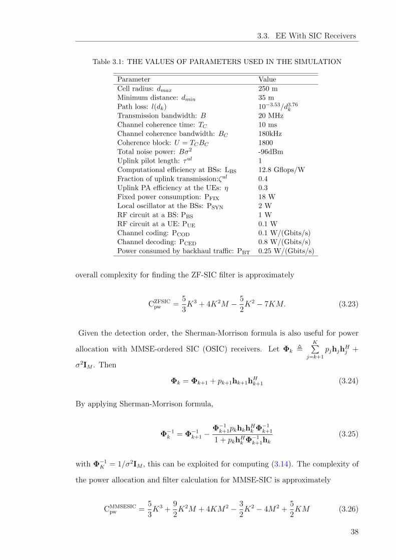
3.3. EE With SIC Receivers
Table 3.1: THE VALUES OF PARAMETERS USED IN THE SIMULATION
Parameter Value
Cell radius: dmax 250 mMinimum distance: dmin 35 mPath loss: l(dk) 10−3.53/d3.76
k
Transmission bandwidth: B 20 MHzChannel coherence time: TC 10 msChannel coherence bandwidth: BC 180kHzCoherence block: U = TCBC 1800Total noise power: Bσ2 -96dBmUplink pilot length: τul 1Computational efficiency at BSs: LBS 12.8 Gflops/WFraction of uplink transmission:ζul 0.4Uplink PA efficiency at the UEs: η 0.3Fixed power consumption: PFIX 18 WLocal oscillator at the BSs: PSYN 2 WRF circuit at a BS: PBS 1 WRF circuit at a UE: PUE 0.1 WChannel coding: PCOD 0.1 W/(Gbits/s)Channel decoding: PCED 0.8 W/(Gbits/s)Power consumed by backhaul traffic: PBT 0.25 W/(Gbits/s)
overall complexity for finding the ZF-SIC filter is approximately
CZFSICpw =
5
3K3 + 4K2M − 5
2K2 − 7KM. (3.23)
Given the detection order, the Sherman-Morrison formula is also useful for power
allocation with MMSE-ordered SIC (OSIC) receivers. Let Φk ,K∑
j=k+1
pjhjhHj +
σ2IM . Then
Φk = Φk+1 + pk+1hk+1hHk+1 (3.24)
By applying Sherman-Morrison formula,
Φ−1k = Φ−1
k+1 −Φ−1k+1pkhkh
Hk Φ−1
k+1
1 + pkhHk Φ−1k+1hk
(3.25)
with Φ−1K = 1/σ2IM , this can be exploited for computing (3.14). The complexity of
the power allocation and filter calculation for MMSE-SIC is approximately
CMMSESICpw =
5
3K3 +
9
2K2M + 4KM2 − 3
2K2 − 4M2 +
5
2KM (3.26)
38
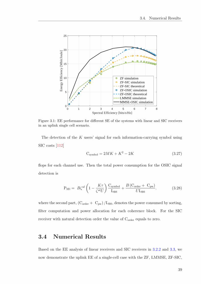
3.4. Numerical Results
0 1 2 3 4 5 6 7 8
Spectral Efficiency [bits/s/Hz]
0
5
10
15
20
25
Ene
rgy
Eff
icie
ncy
[Mbi
t/Jou
le]
ZF simulationZF-SIC simulationZF-SIC theoreticalZF-OSIC simulationZF-OSIC theoreticalLMMSE simulationMMSE-OSIC simulation
Figure 3.1: EE performance for different SE of the systems with linear and SIC receiversin an uplink single cell scenario.
The detection of the K users’ signal for each information-carrying symbol using
SIC costs [112]
Csymbol = 2MK +K2 − 2K (3.27)
flops for each channel use. Then the total power consumption for the OSIC signal
detection is
PSD = Bζul(
1− Kτ
ζulU
)Csymbol
LBS
+B (Corder + Cpw)
ULBS
. (3.28)
where the second part, (Corder + Cpw) /LBS, denotes the power consumed by sorting,
filter computation and power allocation for each coherence block. For the SIC
receiver with natural detection order the value of Corder equals to zero.
3.4 Numerical Results
Based on the EE analysis of linear receivers and SIC receivers in 3.2.2 and 3.3, we
now demonstrate the uplink EE of a single-cell case with the ZF, LMMSE, ZF-SIC,
39
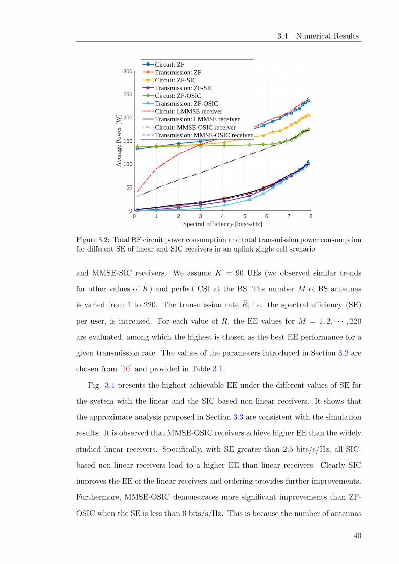
3.4. Numerical Results
0 1 2 3 4 5 6 7 8
Spectral Efficiency [bits/s/Hz]
0
50
100
150
200
250
300
Ave
rage
Pow
er [
W]
Circuit: ZFTransmission: ZFCircuit: ZF-SICTransmission: ZF-SICCircuit: ZF-OSICTransmission: ZF-OSICCircuit: LMMSE receiverTransmission: LMMSE receiverCircuit: MMSE-OSIC receiverTransmission: MMSE-OSIC receiver
Figure 3.2: Total RF circuit power consumption and total transmission power consumptionfor different SE of linear and SIC receivers in an uplink single cell scenario
and MMSE-SIC receivers. We assume K = 90 UEs (we observed similar trends
for other values of K) and perfect CSI at the BS. The number M of BS antennas
is varied from 1 to 220. The transmission rate R, i.e. the spectral efficiency (SE)
per user, is increased. For each value of R, the EE values for M = 1, 2, · · · , 220
are evaluated, among which the highest is chosen as the best EE performance for a
given transmission rate. The values of the parameters introduced in Section 3.2 are
chosen from [10] and provided in Table 3.1.
Fig. 3.1 presents the highest achievable EE under the different values of SE for
the system with the linear and the SIC based non-linear receivers. It shows that
the approximate analysis proposed in Section 3.3 are consistent with the simulation
results. It is observed that MMSE-OSIC receivers achieve higher EE than the widely
studied linear receivers. Specifically, with SE greater than 2.5 bits/s/Hz, all SIC-
based non-linear receivers lead to a higher EE than linear receivers. Clearly SIC
improves the EE of the linear receivers and ordering provides further improvements.
Furthermore, MMSE-OSIC demonstrates more significant improvements than ZF-
OSIC when the SE is less than 6 bits/s/Hz. This is because the number of antennas
40
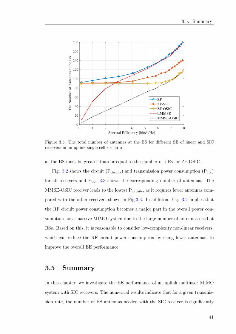
3.5. Summary
0 1 2 3 4 5 6 7 8
Spectral Efficiency [bits/s/Hz]
0
20
40
60
80
100
120
140
160
180
The
Num
ber
of A
nten
nas
at th
e B
S
ZFZF-SICZF-OSICLMMSEMMSE-OSIC
Figure 3.3: The total number of antennas at the BS for different SE of linear and SICreceivers in an uplink single cell scenario
at the BS must be greater than or equal to the number of UEs for ZF-OSIC.
Fig. 3.2 shows the circuit (Pcircuits) and transmission power consumption (PTX)
for all receivers and Fig. 3.3 shows the corresponding number of antennas. The
MMSE-OSIC receiver leads to the lowest Pcircuits, as it requires fewer antennas com-
pared with the other receivers shown in Fig.3.3. In addition, Fig. 3.2 implies that
the RF circuit power consumption becomes a major part in the overall power con-
sumption for a massive MIMO system due to the large number of antennas used at
BSs. Based on this, it is reasonable to consider low-complexity non-linear receivers,
which can reduce the RF circuit power consumption by using fewer antennas, to
improve the overall EE performance.
3.5 Summary
In this chapter, we investigate the EE performance of an uplink multiuser MIMO
system with SIC receivers. The numerical results indicate that for a given transmis-
sion rate, the number of BS antennas needed with the SIC receiver is significantly
41

3.5. Summary
smaller than that with the linear receiver. Therefore, using the SIC based receiver
can reduce the RF circuit power consumption at the BS, and thus improve the overall
EE performance. In light of this, in the next chapter, we study the EE performance
of massive MIMO systems with low-resolution ADCs and SIC receivers.
42
Chapter 4
Energy Efficiency of Uplink Massive
MIMO Systems With Low-Resolution
ADCs and Successive Interference
Cancellation
4.1 Introduction
The study in the last chapter assumed ideal ADCs and perfect CSI. It is unclear
if SIC can also improve the overall EE when low-resolution ADCs are applied to
massive MIMO systems. This chapter intends to answer this question. To do this,
we first derive the optimal power allocation schemes for ZF and ZF-SIC receivers
with ADC quantization errors, under the assumptions of equal-rate transmissions
and the AQNM model. Meanwhile, we derive the analytical approximations to
the power allocation leveraging random matrix theory, which provides a fast and
43
4.2. System Model
accurate characterization of the required transmission power. The cases of perfect
CSI and imperfect CSI obtained using a LMMSE channel estimator from coarsely
quantized observations are both studied. We focus on single-cell scenarios but also
conduct an approximation analysis for multi-cell scenarios. We then adopt a system-
level power consumption model that accounts for both the transmission power and
circuits power such that the EE can be evaluated and optimized. We show by
numerical results that there are scenarios where the circuits power dominates the
overall power consumption due to the deployment of a large number of BS antennas.
In this case, the ZF-SIC receiver may require much fewer antennas as compared
to the ZF receiver, whereas the increase of the power consumption due to digital
signal processing (DSP) is moderate. Consequently, when the number of active
BS antennas can be adapted, the ZF-SIC receiver may improve the overall EE,
benefiting from its capability to achieve a higher SE with limited resources.
This chapter is organized as follows. We introduce the system model of uplink
massive MIMO systems with low-resolution ADCs in Section 4.2. We then derive
the optimal power allocation with low-resolution ADCs and their asymptotic ap-
proximations in Section 4.3. In Section 4.4, we introduce the system-level power
consumption used in this chapter. We present numerical results in Section 4.5 and
conclude the chapter in Section 4.6.
4.2 System Model
In this chapter, we focus on the uplink of a single-cell MIMO system with M BS
antennas and K single-antenna UEs. Assume that the system operates in a TDD
mode as introduced in Section 2.1.1. The slowly varying path loss βk for UE-k due
to large-scale fading is modeled in (2.4). The system model is given by
y = Hx + n =K∑k=1
hkxk + n, (4.1)
44
4.2. System Model
where y ∈ CM is the signal vector observed at the BS, H = [h1,h2, ...,hK ] ∈ CM×K
is the channel matrix, x ∈ CK contains the transmitted symbols xk from the UEs,
and n ∈ CM is the AWGN with variance σ2 (in Joule/symbol). Let hmk be the
(m, k)-th entry of H, denoting the channel gain between the k-th UE and the m-th
BS antenna. Similar to [10], we assume an uncorrelated Rayleigh fading channel
model where hmk are mutually independent of each other, and
hmk ∼ CN (0, βk), ∀m,∀k. (4.2)
Let pk be the transmission power allocated for the UE-k and define
p , [p1, p2, · · · , pK ]T . (4.3)
The received analog signals are sampled and quantized using ADCs. We assume
that ADCs of the same resolution are used at the different BS RF chains. Since a
b-bit ADC employs a finite number (2b) of quantization levels, quantization errors
may arise. Following [70], the quantized signal yq can be modeled using the AQNM,
which decomposes the quantizer output as the summation of the attenuated input
signal and an uncorrelated distortion, i.e.,
yq = αy + nq = αHx + αn + nq, (4.4)
where nq is the additive Gaussian quantization noise which is uncorrelated with y.
Given the number of quantization bits, α can be found as in [70]. The covariance
matrix of nq is
Rnq = E[nqn
Hq |H
]= α (1− α) diag
(HRxH
H + σ2I), (4.5)
where (·)H denotes the Hermitian transpose and Rx is the diagonal covariance matrix
of the transmitted signals, whose k-th diagonal entry represents the average power
45
4.3. Transmit Power Allocation
pk of UE-k’s transmitted signal. In the following, we assume that x, n and nq are
mutually independent, following [38, 70, 78]. This widely adopted assumption leads
to tractable, low-complexity methods for analyzing the performance and designing
the transceivers.
4.3 Transmit Power Allocation
Using a large number of antennas, massive MIMO systems reduce the transmission
power requirement for a given QoS of the UEs. Applying low-resolution ADCs may
improve the overall EE, which also depends on the receiver at the BS. The max-
imum likelihood (ML) receiver achieves channel capacity but its complexity grows
exponentially with K. This chapter considers the low-complexity ZF and ZF-SIC re-
ceivers, which generally outperform MRC-based receivers and require less statistical
knowledge than the LMMSE receivers. In this section, we first derive the power al-
location scheme to support equal-rate transmissions of UEs with ADC quantization
errors and perfect CSI. We then extend the results for the more realistic scenarios
with imperfect CSI obtained from LMMSE channel estimators. For each scenario,
we derive analytical expressions for approximating the required transmission power,
which allows fast analysis and optimization of the system performance. We further
extend the asymptotic analysis to a symmetric multi-cell setting where pilot con-
tamination and inter-cell-interference are taken into account. The results will be
used for analyzing the EE in Section 4.4.
4.3.1 Single-Cell Transmissions With Perfect CSI
In this subsection, we study the power allocation for several ZF-based receivers with
perfect CSI for the single-cell, uplink system described in Section 4.2.
46
4.3. Transmit Power Allocation
4.3.1.1 SE Analysis
When the ZF receiver is used at the BS for recovering information, the estimate of
UE-k’s signal is given as
xk = gHk yq, (4.6)
where yq is the quantized output signal given in (4.4),
gk = [H(HHH
)−1]:,k (4.7)
denotes the ZF weights for UE-k, and [·]:,k denotes taking the k-th column of a
matrix. Applying the AQNM, the estimated signal can be further modeled by
xk = αgHk hkxk + αK∑
n=1,n 6=k
gHk hnxn + αgHk n + gHk nq. (4.8)
When the ZF-SIC receiver is used, we first assume a detection order of UEs
1, 2, · · · , K. Furthermore, we assume that the inter-user-interferences from UE-1 to
UE-(k − 1) are perfectly canceled from yq while detecting UE-k’s signal, resulting
in
yk,q = yq − αk−1∑i=1
hixi = αK∑n=k
hnxn + αn + nq. (4.9)
UE-k’s signal is then estimated as
xk = gHk yk,q, (4.10)
where
gk =[Hk(H
Hk Hk)
−1]
:,1, (4.11)
Hk = [hk,hk+1, · · · ,hK ]. (4.12)
47
4.3. Transmit Power Allocation
The estimate with ZF-SIC can be further written as
xk = αgHk hkxk + α
K∑n=k+1
gHk hnxn + αgHk n + gHk nq. (4.13)
It can be verified that, for the ZF receiver, gHk hk = 1 while gHk hn = 0 for
∀n 6= k. Similarly, for the ZF-SIC receiver, gHk hk = 1 while gHk hn = 0 for ∀n > k.
Therefore, the inter-user-interference is completely mitigated for both the ZF and
ZF-SIC receivers. However, the amplification of the quantization errors and channel
noise is different for the two receivers due to the difference in (4.7) and (4.11).
With the transmission power pk, the achievable gross transmission rate Rk for
UE-k is
Rk = B log (1 + γk) , (4.14)
where the SINR is
γk =α2pkNk
, (4.15)
and Nk denotes the distortion-plus-noise power.
Note that, conditioned on hmn, the power of the quantization noise at the
m-th receiver antenna is given by α (1− α) (K∑n=1
|hmn|2pn + σ2) according to (4.5).
Define D ∈ CK×K whose (k, n)-th entry is
Dkn ,M∑m=1
|g∗kmhmn|2, (4.16)
where gkm is the m-th entry of gk, hmn the m-th entry of hn and ∗ the complex
conjugate. The distortion-plus-noise power Nk is
Nk = α (1−α)K∑n=1
Dknpn+α (1−α) ‖gk‖2σ2+α2‖gk‖2σ2 =α‖gk‖2σ2+α (1−α)K∑n=1
Dknpn,
(4.17)
where gk is given by (4.7) and (4.11), respectively, for the ZF and ZF-SIC receivers.
Given the power allocation vector p, the effective uplink transmission rate of UE-k
48
4.3. Transmit Power Allocation
is
Rk = ζul
(1− τulK
Uζul
)Rk, (4.18)
where 1 − τulKUζul characterizes the decrease of effective transmission rate due to the
training overhead.
4.3.1.2 Transmission Power Allocation
Consider an equal-rate transmission scenario where Rk = R, ∀k. This requires that
each UE must achieve the same SINR γk = 2R/B − 1 after signal detection, i.e.,
2R/B − 1 =α2pk
ασ2‖gk‖2 + α (1− α)K∑n=1
Dknpn
, 1 ≤ k ≤ K.(4.19)
From (4.19), we can write K linear equations with unknowns pk, 1 ≤ k ≤ K, which
can be given alternatively in the matrix-vector form as
α2
2R/B − 1p = ασ2c + α (1− α) Dp, (4.20)
where c ∈ CK with its k-th entry given by ‖gk‖2. After some manipulations, the
optimal power allocation for the UEs can be found as
p = ασ2
[(α2
2R/B − 1
)I− α (1− α) D
]−1
c. (4.21)
This power allocation scheme applies to both the ZF and ZF-SIC receivers. Note
that, however, the expressions of gk are different for the two receivers.
In the above, we have assumed a fixed detection order for the ZF-SIC receivers,
i.e., UE-1 is detected first, followed by UE-2, etc. Optimizing the detection order
can further reduce the transmission power consumption for ZF-SIC receivers. In this
chapter, we consider a norm-based, zero-forcing ordered successive interference can-
cellation (ZF-OSIC) due to its simplicity and good performance: UEs with channel
vectors having larger norms ‖hk‖ are detected earlier.
49
4.3. Transmit Power Allocation
Remark 1 : As a comparison, when the MRC receiver is used, the estimated
signal is similar to (4.8) with gk replaced by
gk = [H]:,k. (4.22)
In this case, the distortion-plus-noise power is given by
Nk = α2
K∑i=1,i 6=k
|gHk hi|2pi + α‖gk‖2σ2 + α (1− α)K∑n=1
Dknpn, (4.23)
which differs from (4.17) in that the inter-user interference can not be perfectly
canceled. In order for the assumed rate to be supported for all UEs, the power
allocation p should satisfy
2R/B − 1 =α2|gHk hk|2pk
Nk
,∀k. (4.24)
Let A ∈ CK×K be a diagonal matrix with its (k, k)-th entry being |gHk hk|2, E ∈
CK×K a matrix whose (k, i)-th entry is |gHk hi|2, and c ∈ CK×1 a vector whose k-th
entry is ‖gk‖2. The power allocation with the MRC receiver is found as
p = ασ2
[(α2
2R/B − 1+ α2
)A− α2E− α (1− α) D
]−1
c. (4.25)
4.3.1.3 Asymptotic Analysis
In this subsection, we perform an asymptotic analysis of the transmitted power
under the large system assumption M →∞, K →∞ with K/M → c, where c is a
constant, in order to obtain fast evaluation of the achievable performance. We first
consider the linear ZF receivers where the SINR given by (4.19) can be written as
2R/B − 1 =α2pk
α2σ2‖gk‖2 + gHk Rnqgk, 1 ≤ k ≤ K. (4.26)
50
4.3. Transmit Power Allocation
From (4.5), the m-th diagonal entry of Rnq is
[Rnq
]mm
= α (1− α)
(K∑n=1
|hmn|2pn + σ2
). (4.27)
As hmn are assumed to be independent variables with zero mean and variance βk,
we have
E[Rnq
]= α (1− α)
(K∑n=1
βnpn + σ2
)IM , (4.28)
where the expectation is taken over the joint distribution of hmn. After approx-
imating Rnq by its expectation in (4.28), the second item in the denominator of
(4.26) can be approximated by
gHk Rnqgk ≈ α (1− α)
(K∑n=1
βnpn + σ2
)‖gk‖2. (4.29)
From random matrix theory [111], [113], HHH is a complex Wishart matrix. For
the ZF receiver of UE-k, the following holds for large M and K [16],
‖gk‖2 =[(
HHH)−1]k,k≈ 1
βk (M −K). (4.30)
With (4.29) and (4.30), the SINR in (4.26) can be approximated by
2R/B − 1 =pkβk (M −K)(
1α− 1)( K∑
n=1
βnpn + σ2
)+ σ2
, 1 ≤ k ≤ K. (4.31)
Let θk , pkβk. Given M,K, βk and σ2, it can be shown that in order to meet
the SINR requirements in (4.31), the following conditions must be satisfied:
θk =(2R/B − 1)
(M −K)
[(1
α− 1
)( K∑n=1
θn + σ2
)+ σ2
]. (4.32)
Note that, the right-hand side (RHS) of (4.32) are the same for all UEs, which
51
4.3. Transmit Power Allocation
indicates that
θk = θzf , ∀k. (4.33)
Substituting (4.33) into (4.32), we can find
θzf =σ2
(M −K) α2R/B−1
−K(1− α). (4.34)
As such, the power allocated to UE-k is approximated by
pk =θzf
βk, 1 ≤ k ≤ K. (4.35)
Clearly, the approximation in (4.35) is independent of the small-scale fading.
We next consider the ZF-SIC receiver, assuming that signals from UE-1 to k− 1
have been perfectly canceled from the received signal at the k-th stage of detection.
Recall that the detector is specified by (4.11) and (4.12). Note that HHk Hk still
follows a complex Wishart distribution, and
‖gk‖2 =[(
HHk Hk
)−1]kk≈ 1
βk (M − (K − k + 1)). (4.36)
Following the similar treatments for the case of the ZF receiver, the SINR for UE-k
can be approximated using (4.28) and (4.36) as
2R/B − 1 ≈ pkβk (M −K + k − 1)(1α− 1)( K∑
n=1
βnpn + σ2
)+ σ2
, 1 ≤ k ≤ K. (4.37)
Similarly to (4.35) and (4.34), the approximate power allocation with ZF-SIC can
be obtained as
pk =θzf−sic
βk(M −K + k − 1), 1 ≤ k ≤ K, (4.38)
where
θzf−sic =σ2
α2R/B−1
− (1− α)K∑n=1
1M−K+n−1
. (4.39)
52
4.3. Transmit Power Allocation
The approximations (4.35) and (4.38) provide fast prediction of the transmission
power given the numbers of UEs K and BS antennas M , number of ADC bits b,
target transmission rate R, and large-scale fading βk. As b increases, α → 1,
the ADC quantization noise diminishes, and the results agrees with Chapter 3. As
M increases, θzf , θzf−sic and the required transmission power pk decreases. In the
asymptotic setting with M →∞, norm-based ordering of ZF-OSIC is equivalent to
ordering the detection according to the large-scale fading βk as ‖hk‖2 →Mβk.
4.3.2 Single-Cell Transmissions With Imperfect CSI
We next consider power allocation with imperfect CSI obtained by training and a
LMMSE channel estimator.
4.3.2.1 SE Analysis
In practical TDD transmissions, the channels may be estimated in a training phase
at the beginning of each block. Assume that UE-k transmits pilot signal xk with
length τulK to the BS. At the BS, the received pilot signal Yt with quantization
errors is given by
Yt = αHX + αNt + Ntq, (4.40)
where X = [x1,x2, · · · ,xK ]T ∈ CK×τulK , Nt and Ntq denote the AWGN and ADC
quantization noise, respectively. We assume orthogonal training, where xk =√τulKptksk,
sk is chosen as the k-th row of the normalized τulK-point discrete Fourier transform
(DFT) matrix with sHk sk = 1, and ptk defines the training power allocated for UE-k.
Let ytk , YtxHk . From the orthogonality of the DFT matrix, we have
ytk = αHXxHk + αNtxHk + Ntqx
Hk = ατulKptkhk + αNtxHk + Nt
qxHk . (4.41)
Recall that for each UE-k, we assume an uncorrelated Rayleigh fading channel
where the entries of hk follow i.i.d. zero-mean Gaussian distribution with variance
53
4.3. Transmit Power Allocation
βk. The LMMSE estimate [114] of hk can be computed as
hk = CHyhC−1
yyytk, (4.42)
where
Cyh , E[hk(ytk)H ] = ατulKβkp
tkIM (4.43)
and
Cyy , E[ytk(ytk)H ]
=
((ατulKptk
)2βk + α2σ2τulKptk + τulKptkα (1− α)
(K∑n=1
βnptn + σ2
))IM .
(4.44)
We can then write the LMMSE estimate of hk as
hk = ψkytk (4.45)
where
ψk =βk
ατulKptkβk + ασ2 + (1− α)
(K∑n=1
βnptn + σ2
) . (4.46)
We assume that a fixed pilot to noise ratio (PNR) χ is achieved for all the UEs by
using appropriate power allocation, i.e.,
ptn =χσ2
βn, n = 1, 2, · · · , K. (4.47)
Define the channel estimation error for UE-k as
ek , hk − hk,∀k. (4.48)
From the orthogonality principle of LMMSE estimators, hk and ek are uncorrelated.
54
4.3. Transmit Power Allocation
From [114], the covariance matrix of ek is computed as
E[ekeHk ] = E[hkh
Hk ]−CH
yhC−1yyCyh. (4.49)
Substituting (4.47) into (4.43) and (4.44) and after some manipulations, (4.49) can
be calculated by
E[ekeHk ] = σ2
ekIM (4.50)
where
σ2ek
= βk(1− ρ) (4.51)
and
ρ =τulKχ
τulKχ+ 1 + ( 1α− 1)(1 +Kχ)
. (4.52)
Furthermore, the variance of the entries of the channel estimate hk is given by
βk = βkρ. (4.53)
From (4.53) and (4.52), the ADC resolution affects the channel estimation accuracy.
When the resolution improves, α increases, ρ increases and σ2e decreases.
Data transmission then follows the training phase. The BS computes the detec-
tors gk using the estimated channel vectors. For the ZF receiver
gk = [H(HHH
)−1
]:,k, (4.54)
which leads to gHk hk = 1 and gHk hn = 0,∀n 6= k. For the ZF-SIC receiver,
gk =[Hk(H
Hk Hk)
−1]
:,1, (4.55)
Hk = [hk, hk+1, · · · , hK ], (4.56)
which leads to gHk hk = 1 while gHk hn = 0,∀n > k. For both receivers, the estimated
55
4.3. Transmit Power Allocation
signal for UE-k can be modeled as
xk = αxk + αK∑n=1
gHk enxn + αgHk n + gHk nq, (4.57)
where the second item at the RHS models the residual error due to imperfect channel
estimation. Since hk and ek are independent, we have gk and en independent,
∀k, ∀n. Given the transmission power p for all the users, the achievable rate for user
k is then computed as
Rk = B log (1 + γk) , (4.58)
where
γk =α2pk
Nk
. (4.59)
and the power of the distortion-plus-noise is computed as
Nk =α2
K∑n=1
|gHk en|2pn + α‖gk‖2σ2 + α (1− α)K∑n=1
Dknpn (4.60)
Dkn ,M∑m=1
|g∗kmhmn|2. (4.61)
4.3.2.2 Transmission Power Allocation
Assuming equal-rate transmission in the data transmission phase, all UEs must have
the same signal-to-noise ratio γk = 2R/B − 1, i.e.,
2R/B − 1 =α2pk
Nk
, 1 ≤ k ≤ K. (4.62)
Note that Nk in (4.60) depends on the unknown channel estimation error. In order to
obtain a practical power allocation scheme, we approximate the term enxn in (4.57)
due to the channel estimation error as an independent noise with zero mean and
variance σ2enpn. Accordingly, we approximate the power received at BS antenna m as
56
4.3. Transmit Power Allocation
∑Kn=1
(|hmn|2 + σ2
en
)pn. As such, we can approximate the power of the distortion-
plus-noise in (4.60) as
Nk≈α2‖gk‖2
K∑n=1
σ2enpn + α‖gk‖2σ2 + α (1− α)
K∑n=1
Dk,npn
where
Dkn ≈M∑m=1
|g∗km|2(|hmn|2 + σ2
en
). (4.63)
It can be shown that such approximations yield negligible loss in accuracy for large
systems. We can rearrange the linear equations in (4.62) in a matrix-vector form as
α2
2R/B − 1p = ασ2c + α2Jp + α(1− α)Dp (4.64)
where the entries of D, J and c are given by Dkn, Jki , ‖gk‖2σ2ei
, and ck , ‖gk‖2,
respectively. After some manipulations, the power allocation for the UEs with im-
perfect CSI can be found as
p = ασ2
[(α2
2R/B − 1
)I− α2J− α (1− α) D
]−1
c. (4.65)
Similar to the case of perfect CSI introduced in Section 4.3.1, the order of the
ZF-SIC detection can be optimized to reduce the transmit power. Specifically, the
norm-based ordering based on ‖hk‖2 is equivalent to ordering based on βk in the
large system regime.
4.3.2.3 Asymptotic Analysis
For the asymptotic analysis of the transmission power, we start with the ZF re-
ceiver. Similar to (4.26)-(4.29), we approximate the quantization noise power by its
expectation as in (4.28). With the LMMSE channel estimator and the ZF detector,
57
4.3. Transmit Power Allocation
the SINR for UE-k (4.62) can be approximated as
2R/B−1 ≈ pk
σ2‖gk‖2 + ‖gk‖2K∑n=1
σ2enpn +
(1α− 1)‖gk‖2
(K∑n=1
βnpn + σ2
) , 1 ≤ k ≤ K.
(4.66)
Since the entries of hk follows i.i.d., complex Gaussian distribution with zero mean
and variance βk, HHH still holds a complex Wishart distribution. The detector gk
of UE-k can be treated similarly to the case with perfect CSI as
‖gk‖2 =
[(HHH
)−1]kk
≈ 1
βk (M −K). (4.67)
By substituting (4.67) into (4.66), the SINR for UE-k can be approximated by
2R/B − 1 ≈ pkβk (M −K)(1α− 1)( K∑
n=1
βnpn + σ2
)+
K∑n=1
(βn − βn)pn + σ2
, 1 ≤ k ≤ K, (4.68)
where we have used the fact that βn = ρβn, σ2en = (1− ρ)βn,∀n.
Similarly to the case of perfect CSI, the optimal power allocation with the ZF
receiver based on the estimated channel is given by
pk =θzf
βk,∀k, (4.69)
with θ being a constant that is independent of k. Substituting (4.69) into (4.68), we
have
θzf =σ2
(M −K) α2R/B−1
− 1ρK(1− αρ)
. (4.70)
The case with ZF-SIC can be analyzed by using
‖gk‖2 ≈ 1
βk (M − (K − k + 1)). (4.71)
58
4.3. Transmit Power Allocation
Substituting (4.71) into (4.66), the SINR approximation for UE-k is
2R/B − 1 ≈ pkβk (M −K + k − 1)(1α− 1)( K∑
n=1
βnpn + σ2
)+
K∑n=1
pn(βn − βn) + σ2
, 1 ≤ k ≤ K. (4.72)
Following a similar method as for the case with perfect CSI, the power allocation
with the ZF-SIC and imperfect CSI can be written as
pk =θzf−sic
βk(M −K + k − 1),∀k (4.73)
where
θzf−sic =σ2
α2R/B−1
− 1ρ(1− αρ)
K∑n=1
1M−K+n−1
. (4.74)
It can be verified that the solutions in (4.69) and (4.73) for the imperfect CSI case
reduce to the solution for the case of perfect CSI in (4.35) and (4.38) by letting
ρ = 1.
Remark 2 : The approximations to the transmission power in this section have
good accuracies for moderate-to-large M , as will be shown by the numerical results.
This provides useful tools for fast evaluation and optimization of the performance.
Similar approximation analysis has been conducted for massive MIMO systems. For
example, [16] and [10] considered, respectively, equal-power and equal-rate transmis-
sions for several linear receivers with ideal ADCs; [70] analyzed the MRC receiver
with equal-power transmission, perfect CSI and low-resolution ADCs; [115] and [38]
considered imperfect CSI and general fading channels; and [78] studied LMMSE
receivers with perfect CSI and mixed-ADCs. This chapter provides new results for
the ZF and ZF-SIC receivers with low-resolution ADCs, equal-rate transmissions,
and imperfect channel estimation.
59
4.3. Transmit Power Allocation
4.3.3 Asymptotic Analysis for Multiple-Cell Transmissions
In the above, the power allocation and their asymptotic approximations have been
derived for the ZF and ZF-SIC receivers in a single-cell setting. We now extend the
asymptotic analysis to multi-cell systems. Following [10], we consider a system with
L symmetric square cells, where the ADC resolutions, the number of BS antennas,
the UE distributions and transmission rates are exactly the same in all cells. We
now study the asymptotic power allocation that takes into account the quantization
errors, channel estimation errors, and inter-cell-interference.
We fist consider the training phase and analyze the channel estimation perfor-
mance. Following [10], the quantized received training signal at the BS in cell-j can
be modeled as
Ytj = α
L∑l=1
K∑k=1
hj,l,kxtl,k + αNt
j + Ntq,j, (4.75)
where hj,l,k denotes the channel vector between UE-k of cell l and the BS of cell j, Ntj
and Ntq,j denote the channel noise and quantization noise, respectively. Similar to
the single-cell case in Section 4.3.2, we assume that orthogonal pilots are used within
each cell, where the pilot signal for UE-k in cell l is given by xl,k =√τulKptl,ksl,k,
where ptl,k denotes the transmission power. Meanwhile, in order to accommodate
the LK UEs in the whole system, the training waveforms sl,k of length τulK are
reused in a subset (L) of cells, following [116]. This leads to pilot contamination.
From the symmetric assumption, the large-scale fading βl,l,k is independent of the
cell index l and the PNR of all the UEs at their serving BS is fixed to χ. As such,
the pilot power is allocated as
ptl,k =χσ2
βl,l,k, l = 1, 2, · · · , L, k = 1, 2, · · · , K, (4.76)
where σ2 is the receiver noise power. The corresponding quantization noise power
60
4.3. Transmit Power Allocation
at the j-th BS receiver is then given by
σ2q = α(1− α)
(L∑l=1
K∑n=1
βj,l,nptl,n + σ2
). (4.77)
Note that due to the symmetric assumption, βl,l,k, ptl,k, xl,k, σ
2 and σ2q are indepen-
dent of l.
Now consider the LMMSE estimation of the channel for UE-k of cell j. Define
ytj,k , Ytjx
Hj,k. (4.78)
From (4.75) and the assumptions about the pilot assignments, the received signal
contains the channel noise, quantization noise and also the interference from UEs of
other cells that use the same pilot xj,k.
ytj,k = ατulKptj,k∑l∈L
hj,l,k + αNtxHj,k + Ntq,jx
Hj,k. (4.79)
Assuming uncorrelated Rayleigh fading, we have
Cyh , E[ytj,khHj,j,k] = ατulKptj,kβj,j,kI. (4.80)
Cyy , E[ytj,k(ytj,k)
H ] =
((ατulKptj,k
)2∑l∈L
βj,l,k + τulKptj,k(α2σ2 + σ2
q
))I. (4.81)
The LMMSE estimate of hj,j,k is now computed as
hj,j,k = CHyhC−1
yyytj,k = ψkytj,k, (4.82)
61
4.3. Transmit Power Allocation
where the scaling factor
ψk =ατulKptj,kβj,j,k(
ατulKptj,k)2 ∑
l∈Lβj,l,k + τulKptj,k
(α2σ2 + σ2
q
) (4.83)
(4.77)=
βj,j,k
(ατulK)∑l∈L
βj,l,kptj,k + 1α
(ασ2 + α(1− α)
(L∑l=1
K∑n=1
βj,l,nptl,n
)) (4.84)
In order to gain insights with tractable analysis, we follow [10] to assume that
βj,l,n = γj,lβj,j,n, ∀l,∀n, (4.85)
where γj,l is the expectation of the ratio of path losses
γj,l , E[βj,l,kβj,j,k
]. (4.86)
Furthermore, let us define
ΓL =L∑
l=1,l 6=j
γj,l, ΓL =∑
l∈L,l 6=j
γj,l. (4.87)
It can be now verified that
βj,l,kptj,k = γj,lβj,j,kp
tj,k = γj,lχσ
2, ∀k. (4.88)
We can then rewrite (4.83) as
ψk =βj,j,k
ατulKχσ2(1 + ΓL) + σ2 + (1− α)K(1 + ΓL)χσ2, (4.89)
which indicates that the LMMSE estimator depends on the path losses, target PNR,
quantization noise and pilot contamination. Given the above LMMSE estimation,
the channel estimation errors for UE-k in cell-j follows an i.i.d. distribution with
62
4.3. Transmit Power Allocation
covariance matrix
Ehj,k = βj,j,kI−CH
yhC−1yyCyh =
(βj,j,k − ατulKβj,j,kp
tj,kψk
)I = σ2
ej,kI, (4.90)
where
σ2ej,k
= (1− ρmc)βj,j,k, (4.91)
and
ρmc =τulKχ
τulKχ(1 + ΓL) + 1α
+K(
1α− 1)
(ΓL + 1)χ. (4.92)
Note that by letting ΓL = 0 and ΓL = 0 (4.92) reduces to (4.52) when there is
no pilot contamination and inter-cell-interference. Furthermore, the entries of the
estimated channel vector hj,j,k are i.i.d., with variance
βj,j,k = ρmcβj,j,k. (4.93)
Now let us consider the data transmission phase where LK users are transmitting
simultaneously. The received signal at the BS of cell-j is modeled as
yj = αL∑l=1
K∑n=1
hj,l,nxl,n + αnj + nq,j, (4.94)
where nq,j and nj are quantization noise and AWGN with variance of
α(1− α)
(L∑l=1
K∑n=1
βj,l,npn + σ2
)
and σ2 and pn is the power of the n-th UE of each cell. Let gj,j,k be the (ZF or
ZF-SIC) receiver weights for UE-k of cell j constructed from the LMMSE chan-
nel estimates with the channel estimation errors ignored. Treating the inter-cell-
interference, error due to imperfect CSI, and quantization noise as AWGN, the
63
4.3. Transmit Power Allocation
following should be satisfied
2R/B − 1 ≈ α2pk‖gj,j,k‖2
1
Nmc
, 1 ≤ k ≤ K, (4.95)
where the interference-plus-noise power, which is independent of the target user, is
Nmc =
α2
K∑n=1
σ2ej,npn+α2
L∑l=1,l 6=j
K∑n=1
γj,lβj,j,npn+α2σ2+α(1−α)
(L∑l=1
K∑n=1
γj,lβj,j,npn + σ2
).
(4.96)
For the ZF receiver, by utilizing the approximation in (4.93), ‖gj,j,k‖2 = 1
βj,j,k(M−K).
The transmitted power satisfies
pk =θmc,zf
βj,j,k, ∀k, (4.97)
where it is seen that the transmitted power is inversely proportional to βj,j,k. Sub-
stituting (4.97) into (4.96) and (4.95), we can find
θmc,zf =σ2
(M −K) α2R/B−1
− Kρmc
(ΓL + 1− αρmc). (4.98)
When the ZF-SIC receiver is used, we have ‖gj,j,k‖2 = 1
βj,j,k(M−K+k−1). From (4.95),
the power allocation is approximated as
pk =θmc,zf−sic
βj,j,k(M −K + k − 1),∀k, (4.99)
which suggests that pkβj,j,k =θmc,zf−sic
M−K+k−1,∀k. Similarly, plugging the above into (4.96)
and (4.95), we have
θmc,zf−sic =σ2
α2R/B−1
− 1ρmc
(ΓL + 1− αρmc)∑K
n=11
M−K+n−1
. (4.100)
64
4.4. Energy Efficiency
4.4 Energy Efficiency
Following the power consumption model in [10], we next discuss the EE performance
achieved with the ZF and ZF-SIC receivers, which is measured by the number of
bits transmitted per Joule:
EE =
∑Kk=1Rk
Ptotal
, (4.101)
where Rk denotes the effective transmission rate of UE-k and Ptotal is the average
total power consumption. We focus again on single-cell uplink transmissions and
the analysis is easily applied to the multi-cell case considered in Section 4.3.3.
Specifically, we assume that the transmission rates Rk are given and the total
power consumption
Ptotal = M(PBS + 2PADC) +KPUE + PSYN + Pother + PCD + PDT + PCE + PSD,
(4.102)
where PBS,PUE,PSYN,PCD are the power consumption per RF circuit at the BS,
UE, the local oscillator at the BS, channel coding and decoding respectively and
Pother denotes the backhaul power consumption and the power of site cooling, etc
[10].
The average uplink data transmission power PDT describes the power consumed
by the power amplifiers at the UEs, which includes the dissipation power and trans-
mission power in the data transmission phase. Let η be the power amplifier efficiency
at each UE. Then we have
PDT =Bζul
η
(1− τulK
Uζul
)E1T
Kp, (4.103)
where p in Joule/symbol is the power allocation vector as discussed in Section 4.3.
The power consumed by channel estimation during the training phase (PCE) con-
sists of the pilots transmission power (PCE−Pilots) and the DSP power consumption
for channel estimation (PCE−SP). In the uplink transmission under the TDD proto-
65

4.4. Energy Efficiency
col, there are B/U coherence blocks per second and the LMMSE channel estimation
is performed once per block. Following Section III, each UE transmits its pilot signal
xk of length τulK with a power of ptk. The total pilots transmission power is given
as
PCE−Pilots =BτulK
ηU
K∑k=1
ptk. (4.104)
As introduced regarding (4.47), we assume that ptk are chosen such that the PNR
at the BS is equal to χ for all UEs.
The DSP power consumption during channel training phase PCE−SP depends on
the complexity of the channel estimator. With the LMMSE estimate hk of hk as
discussed in Section 4.3.2. The computational complexity is mainly contributed by
the matrix-vector multiplications for finding ytk in (4.41), which requires 2τulKM
flops for each UE. Then hk can be estimated by applying (4.45), which requires
2K + M flops. To sum up, estimating the K UEs’ channel cost approximately
CCE = 2τulK2M + 2K2 +MK flops. Therefore, the total DSP power consumption
for channel estimation is
PCE−SP =B
U
CCE
LBS
, (4.105)
where LBS represents the computational efficiency at the BS.
Following [99], the power consumption of a b-bits ADC is evaluated by
PADC = FOM · fs · 2b, (4.106)
where the FOM means energy consumed per conversion step, fs the sampling rate.
Generally, an ADC with high resolution leads to smaller quantization errors com-
pared with a low-resolution ADC but also greater power consumption (4.106). The
FOM has been improved in the last decades [100]. As explained in Section 2.4.2.3,
we assume a moderate value of FOM = 1432.1 fJ per conversion step [100] to model
commercialized ADCs.
The signal detection power PSD depends on the complexity of finding the weight
66
4.4. Energy Efficiency
matrix, power allocation and symbol detection, which depend on the type of the
receiver used. Let us begin with the ZF receivers. Calculating the ZF weights (4.54)
for the K UEs requires an approximate complexity of [10]
Cwm−zf =1
3K3 + 3K2M +KM − 1
3K flops. (4.107)
According to (4.65), the complexity for power allocation for the case of imperfect
CSI arises from finding c, D and J, which is approximately Cpower allocation = 23K3 +
3K2M + 7KM + 52K2 − 13
6K flops. Given the weight matrix, the detection of K
UEs’ signals for each information-carrying symbol using ZF costs [10]
Csymbol−zf = 2KM −K flops. (4.108)
We next consider the ZF-SIC receiver. Assuming perfect interference cancellation,
the signal estimate in (4.10) can be computed alternatively as
xk = gHk
(yq − α
k−1∑n=1
hnxn
)= gHk yq −
k−1∑n=1
fknxn, (4.109)
where
fkn = αgHk hn, k = 2, 3, · · · , K, n = 1, 2 · · · , k − 1. (4.110)
If norm-based ordering is applied, computing and sorting ‖hk‖2 has a complexity
of Corder = K2 + 2MK flops [117, 118]. Giving a decoding order, the Sherman-
Morrison formula can be used for computing the receiver weights gk (4.11) for each
UE [112], which requires about 76K3 + 2K2M flops. The computation of (4.110)
requires K2M + K2/2 flops. Summarizing, the total computational complexity for
obtaining gk and fkn is approximately
Cwm−sic =7
6K3 + 3K2M − 3
2K2 +
5
2KM flops, (4.111)
which is shared by the coherent block. The computational complexity of power
67
4.5. Numerical Results
allocation for the ZF-SIC receiver is the same as that for the ZF receiver. Given
gk and fkn, the detection of the K UEs’ signal for each information-carrying
symbol using (4.109) costs about
Csymbol−sic = 2MK +K2 − 2K flops (4.112)
Summarizing, the power consumption of weight matrix computation and power
allocation within each block for ZF and ZF-SIC is
PBL =B (Corder + Cwm + Cpower allocation)
ULBS
, (4.113)
Note that, the linear ZF and ZF-SIC receivers without optimized ordering optimiza-
tion do not require any computation for ordering, i.e. Corder = 0. The total power
consumption for ZF and ZF-SIC signal detection is
PSD = Bζul
(1− Kτul
ζulU
)Csymbol
LBS+ PBL, (4.114)
4.5 Numerical Results
We now present numerical results to demonstrate the influence of low-resolution
ADCs and signal processing methods on the uplink EE of massive MIMO systems.
The values of key model parameters introduced in Sections 4.2 and 4.4 are given
in Table 3.1 following [10], where the RF circuit power at the BS PBS = 0.4 W
is modified from [10] by excluding the relevant ADCs power consumption. Other
values such as PUE,PSYN,Pother, and PCD are set the same as in [10]. Nyquist-rate
sampling is assumed for the ADCs and the PNR in the channel estimation phase
equals to χ = 4 dB. We define SE = R/B and assume all UEs achieve the same SE.
68
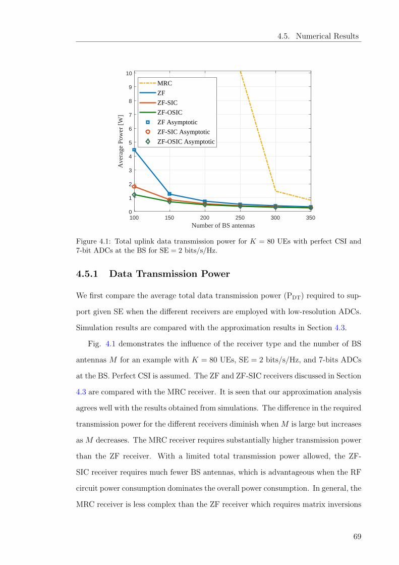
4.5. Numerical Results
100 150 200 250 300 350
Number of BS antennas
0
1
2
3
4
5
6
7
8
9
10
Ave
rage
Pow
er [
W]
MRC
ZF
ZF-SIC
ZF-OSIC
ZF Asymptotic
ZF-SIC Asymptotic
ZF-OSIC Asymptotic
Figure 4.1: Total uplink data transmission power for K = 80 UEs with perfect CSI and7-bit ADCs at the BS for SE = 2 bits/s/Hz.
4.5.1 Data Transmission Power
We first compare the average total data transmission power (PDT) required to sup-
port given SE when the different receivers are employed with low-resolution ADCs.
Simulation results are compared with the approximation results in Section 4.3.
Fig. 4.1 demonstrates the influence of the receiver type and the number of BS
antennas M for an example with K = 80 UEs, SE = 2 bits/s/Hz, and 7-bits ADCs
at the BS. Perfect CSI is assumed. The ZF and ZF-SIC receivers discussed in Section
4.3 are compared with the MRC receiver. It is seen that our approximation analysis
agrees well with the results obtained from simulations. The difference in the required
transmission power for the different receivers diminish when M is large but increases
as M decreases. The MRC receiver requires substantially higher transmission power
than the ZF receiver. With a limited total transmission power allowed, the ZF-
SIC receiver requires much fewer BS antennas, which is advantageous when the RF
circuit power consumption dominates the overall power consumption. In general, the
MRC receiver is less complex than the ZF receiver which requires matrix inversions
69
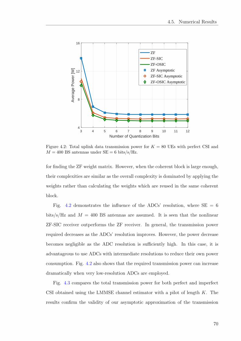
4.5. Numerical Results
3 4 5 6 7 8 9 10 11 12
Number of Quantization Bits
4
8
12
16
Ave
rage
Pow
er [W
]
ZF
ZF-SIC
ZF-OSIC
ZF Asymptotic
ZF-SIC Asymptotic
ZF-OSIC Asymptotic
Figure 4.2: Total uplink data transmission power for K = 80 UEs with perfect CSI andM = 400 BS antennas under SE = 6 bits/s/Hz.
for finding the ZF weight matrix. However, when the coherent block is large enough,
their complexities are similar as the overall complexity is dominated by applying the
weights rather than calculating the weights which are reused in the same coherent
block.
Fig. 4.2 demonstrates the influence of the ADCs’ resolution, where SE = 6
bits/s/Hz and M = 400 BS antennas are assumed. It is seen that the nonlinear
ZF-SIC receiver outperforms the ZF receiver. In general, the transmission power
required decreases as the ADCs’ resolution improves. However, the power decrease
becomes negligible as the ADC resolution is sufficiently high. In this case, it is
advantageous to use ADCs with intermediate resolutions to reduce their own power
consumption. Fig. 4.2 also shows that the required transmission power can increase
dramatically when very low-resolution ADCs are employed.
Fig. 4.3 compares the total transmission power for both perfect and imperfect
CSI obtained using the LMMSE channel estimator with a pilot of length K. The
results confirm the validity of our asymptotic approximation of the transmission
70
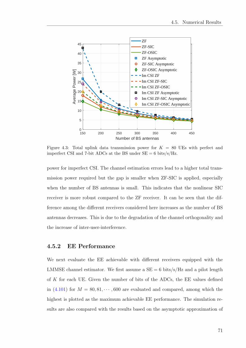
4.5. Numerical Results
150 200 250 300 350 400 450
Number of BS antennas
0
5
10
15
20
25
30
35
40
45
Ave
rage
Pow
er [W
]
ZF
ZF-SIC
ZF-OSIC
ZF Asymptotic
ZF-SIC Asymptotic
ZF-OSIC Asymptotic
Im CSI ZF
Im CSI ZF-SIC
Im CSI ZF-OSIC
Im CSI ZF Asymptotic
Im CSI ZF-SIC Asymptotic
Im CSI ZF-OSIC Asymptotic
Figure 4.3: Total uplink data transmission power for K = 80 UEs with perfect andimperfect CSI and 7-bit ADCs at the BS under SE = 6 bits/s/Hz.
power for imperfect CSI. The channel estimation errors lead to a higher total trans-
mission power required but the gap is smaller when ZF-SIC is applied, especially
when the number of BS antennas is small. This indicates that the nonlinear SIC
receiver is more robust compared to the ZF receiver. It can be seen that the dif-
ference among the different receivers considered here increases as the number of BS
antennas decreases. This is due to the degradation of the channel orthogonality and
the increase of inter-user-interference.
4.5.2 EE Performance
We next evaluate the EE achievable with different receivers equipped with the
LMMSE channel estimator. We first assume a SE = 6 bits/s/Hz and a pilot length
of K for each UE. Given the number of bits of the ADCs, the EE values defined
in (4.101) for M = 80, 81, · · · , 600 are evaluated and compared, among which the
highest is plotted as the maximum achievable EE performance. The simulation re-
sults are also compared with the results based on the asymptotic approximation of
71
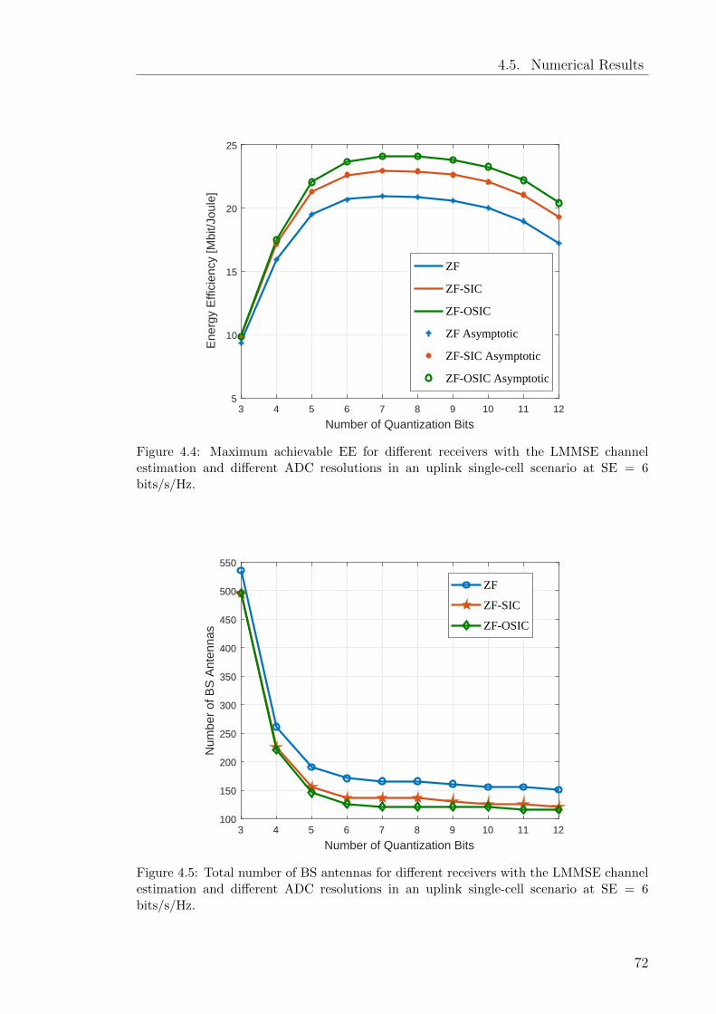
4.5. Numerical Results
3 4 5 6 7 8 9 10 11 12
Number of Quantization Bits
5
10
15
20
25
Ene
rgy
Effi
cien
cy [M
bit/J
oule
]
ZF
ZF-SIC
ZF-OSIC
ZF Asymptotic
ZF-SIC Asymptotic
ZF-OSIC Asymptotic
Figure 4.4: Maximum achievable EE for different receivers with the LMMSE channelestimation and different ADC resolutions in an uplink single-cell scenario at SE = 6bits/s/Hz.
3 4 5 6 7 8 9 10 11 12
Number of Quantization Bits
100
150
200
250
300
350
400
450
500
550
Num
ber
of B
S A
nten
nas
ZF
ZF-SIC
ZF-OSIC
Figure 4.5: Total number of BS antennas for different receivers with the LMMSE channelestimation and different ADC resolutions in an uplink single-cell scenario at SE = 6bits/s/Hz.
72
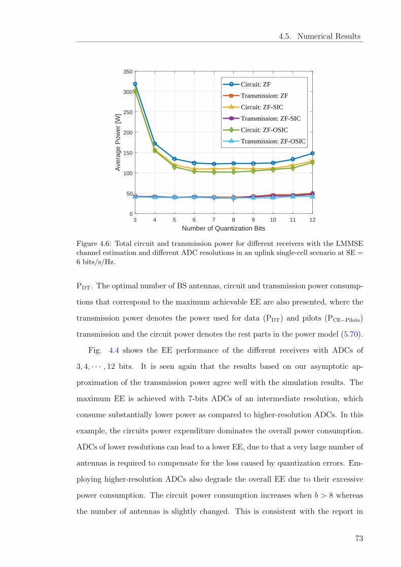
4.5. Numerical Results
3 4 5 6 7 8 9 10 11 12
Number of Quantization Bits
0
50
100
150
200
250
300
350
Ave
rage
Pow
er [W
]
Circuit: ZF
Transmission: ZF
Circuit: ZF-SIC
Transmission: ZF-SIC
Circuit: ZF-OSIC
Transmission: ZF-OSIC
Figure 4.6: Total circuit and transmission power for different receivers with the LMMSEchannel estimation and different ADC resolutions in an uplink single-cell scenario at SE =6 bits/s/Hz.
PDT. The optimal number of BS antennas, circuit and transmission power consump-
tions that correspond to the maximum achievable EE are also presented, where the
transmission power denotes the power used for data (PDT) and pilots (PCE−Pilots)
transmission and the circuit power denotes the rest parts in the power model (5.70).
Fig. 4.4 shows the EE performance of the different receivers with ADCs of
3, 4, · · · , 12 bits. It is seen again that the results based on our asymptotic ap-
proximation of the transmission power agree well with the simulation results. The
maximum EE is achieved with 7-bits ADCs of an intermediate resolution, which
consume substantially lower power as compared to higher-resolution ADCs. In this
example, the circuits power expenditure dominates the overall power consumption.
ADCs of lower resolutions can lead to a lower EE, due to that a very large number of
antennas is required to compensate for the loss caused by quantization errors. Em-
ploying higher-resolution ADCs also degrade the overall EE due to their excessive
power consumption. The circuit power consumption increases when b > 8 whereas
the number of antennas is slightly changed. This is consistent with the report in
73
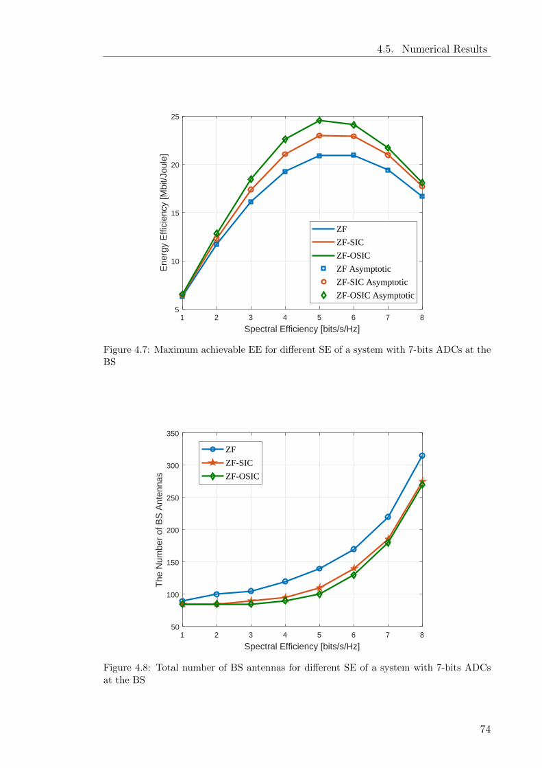
4.5. Numerical Results
1 2 3 4 5 6 7 8
Spectral Efficiency [bits/s/Hz]
5
10
15
20
25
Ene
rgy
Effi
cien
cy [M
bit/J
oule
]
ZF
ZF-SIC
ZF-OSIC
ZF Asymptotic
ZF-SIC Asymptotic
ZF-OSIC Asymptotic
Figure 4.7: Maximum achievable EE for different SE of a system with 7-bits ADCs at theBS
1 2 3 4 5 6 7 8
Spectral Efficiency [bits/s/Hz]
50
100
150
200
250
300
350
The
Num
ber
of B
S A
nten
nas
ZF
ZF-SIC
ZF-OSIC
Figure 4.8: Total number of BS antennas for different SE of a system with 7-bits ADCsat the BS
74
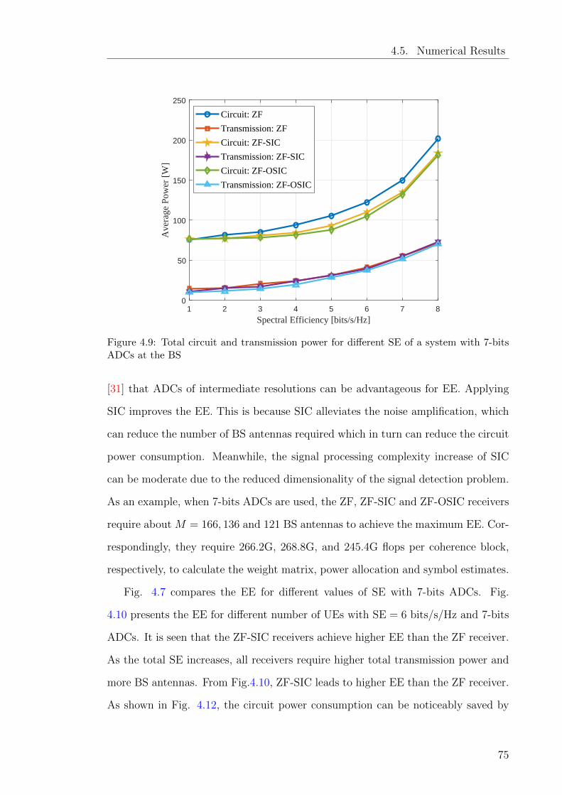
4.5. Numerical Results
1 2 3 4 5 6 7 8
Spectral Efficiency [bits/s/Hz]
0
50
100
150
200
250
Ave
rage
Pow
er [
W]
Circuit: ZF
Transmission: ZF
Circuit: ZF-SIC
Transmission: ZF-SIC
Circuit: ZF-OSIC
Transmission: ZF-OSIC
Figure 4.9: Total circuit and transmission power for different SE of a system with 7-bitsADCs at the BS
[31] that ADCs of intermediate resolutions can be advantageous for EE. Applying
SIC improves the EE. This is because SIC alleviates the noise amplification, which
can reduce the number of BS antennas required which in turn can reduce the circuit
power consumption. Meanwhile, the signal processing complexity increase of SIC
can be moderate due to the reduced dimensionality of the signal detection problem.
As an example, when 7-bits ADCs are used, the ZF, ZF-SIC and ZF-OSIC receivers
require about M = 166, 136 and 121 BS antennas to achieve the maximum EE. Cor-
respondingly, they require 266.2G, 268.8G, and 245.4G flops per coherence block,
respectively, to calculate the weight matrix, power allocation and symbol estimates.
Fig. 4.7 compares the EE for different values of SE with 7-bits ADCs. Fig.
4.10 presents the EE for different number of UEs with SE = 6 bits/s/Hz and 7-bits
ADCs. It is seen that the ZF-SIC receivers achieve higher EE than the ZF receiver.
As the total SE increases, all receivers require higher total transmission power and
more BS antennas. From Fig.4.10, ZF-SIC leads to higher EE than the ZF receiver.
As shown in Fig. 4.12, the circuit power consumption can be noticeably saved by
75
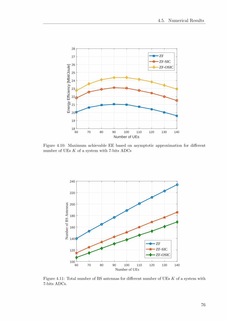
4.5. Numerical Results
60 70 80 90 100 110 120 130 140
Number of UEs
18
19
20
21
22
23
24
25
26
27
28
Ene
rgy
Effi
cien
cy [M
bit/J
oule
]
ZF
ZF-SIC
ZF-OSIC
Figure 4.10: Maximum achievable EE based on asymptotic approximation for differentnumber of UEs K of a system with 7-bits ADCs
60 70 80 90 100 110 120 130 140
Number of UEs
100
120
140
160
180
200
220
240
Num
ber
of B
S A
nten
nas
ZF
ZF-SIC
ZF-OSIC
Figure 4.11: Total number of BS antennas for different number of UEs K of a system with7-bits ADCs.
76
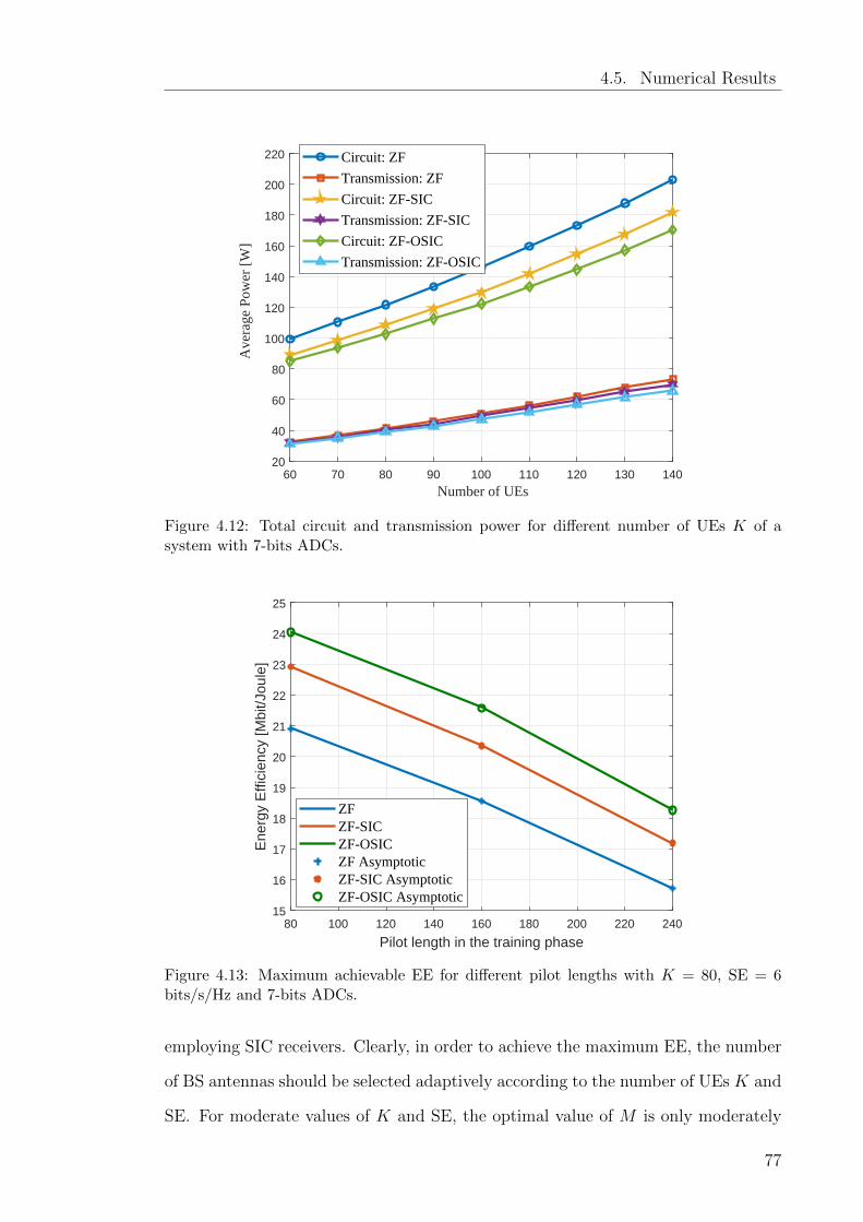
4.5. Numerical Results
60 70 80 90 100 110 120 130 140
Number of UEs
20
40
60
80
100
120
140
160
180
200
220
Ave
rage
Pow
er [
W]
Circuit: ZF
Transmission: ZF
Circuit: ZF-SIC
Transmission: ZF-SIC
Circuit: ZF-OSIC
Transmission: ZF-OSIC
Figure 4.12: Total circuit and transmission power for different number of UEs K of asystem with 7-bits ADCs.
80 100 120 140 160 180 200 220 240
Pilot length in the training phase
15
16
17
18
19
20
21
22
23
24
25
Ene
rgy
Effi
cien
cy [M
bit/J
oule
]
ZFZF-SICZF-OSICZF AsymptoticZF-SIC AsymptoticZF-OSIC Asymptotic
Figure 4.13: Maximum achievable EE for different pilot lengths with K = 80, SE = 6bits/s/Hz and 7-bits ADCs.
employing SIC receivers. Clearly, in order to achieve the maximum EE, the number
of BS antennas should be selected adaptively according to the number of UEs K and
SE. For moderate values of K and SE, the optimal value of M is only moderately
77
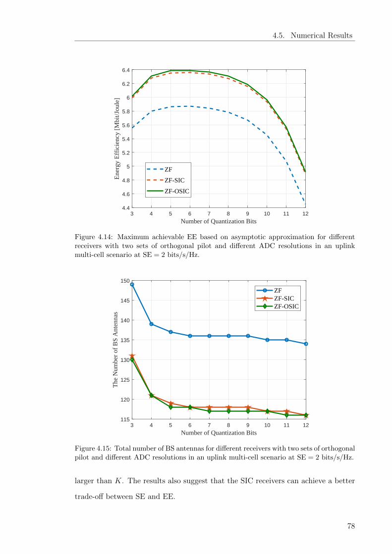
4.5. Numerical Results
3 4 5 6 7 8 9 10 11 12
Number of Quantization Bits
4.4
4.6
4.8
5
5.2
5.4
5.6
5.8
6
6.2
6.4
Ene
rgy
Eff
icie
ncy
[Mbi
t/Jou
le]
ZF
ZF-SIC
ZF-OSIC
Figure 4.14: Maximum achievable EE based on asymptotic approximation for differentreceivers with two sets of orthogonal pilot and different ADC resolutions in an uplinkmulti-cell scenario at SE = 2 bits/s/Hz.
3 4 5 6 7 8 9 10 11 12
Number of Quantization Bits
115
120
125
130
135
140
145
150
The
Num
ber
of B
S A
nten
nas
ZFZF-SICZF-OSIC
Figure 4.15: Total number of BS antennas for different receivers with two sets of orthogonalpilot and different ADC resolutions in an uplink multi-cell scenario at SE = 2 bits/s/Hz.
larger than K. The results also suggest that the SIC receivers can achieve a better
trade-off between SE and EE.
78
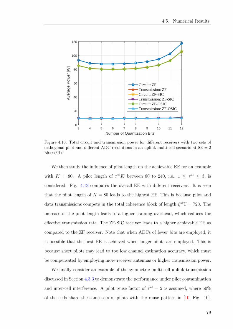
4.5. Numerical Results
3 4 5 6 7 8 9 10 11 12
Number of Quantization Bits
0
20
40
60
80
100
120
Ave
rage
Pow
er [W
]
Circuit: ZFTransmission: ZFCircuit: ZF-SICTransmission: ZF-SICCircuit: ZF-OSICTransmission: ZF-OSIC
Figure 4.16: Total circuit and transmission power for different receivers with two sets oforthogonal pilot and different ADC resolutions in an uplink multi-cell scenario at SE = 2bits/s/Hz.
We then study the influence of pilot length on the achievable EE for an example
with K = 80. A pilot length of τulK between 80 to 240, i.e., 1 ≤ τul ≤ 3, is
considered. Fig. 4.13 compares the overall EE with different receivers. It is seen
that the pilot length of K = 80 leads to the highest EE. This is because pilot and
data transmissions compete in the total coherence block of length ζulU = 720. The
increase of the pilot length leads to a higher training overhead, which reduces the
effective transmission rate. The ZF-SIC receiver leads to a higher achievable EE as
compared to the ZF receiver. Note that when ADCs of fewer bits are employed, it
is possible that the best EE is achieved when longer pilots are employed. This is
because short pilots may lead to too low channel estimation accuracy, which must
be compensated by employing more receiver antennas or higher transmission power.
We finally consider an example of the symmetric multi-cell uplink transmission
discussed in Section 4.3.3 to demonstrate the performance under pilot contamination
and inter-cell interference. A pilot reuse factor of τul = 2 is assumed, where 50%
of the cells share the same sets of pilots with the reuse pattern in [10, Fig. 10].
79
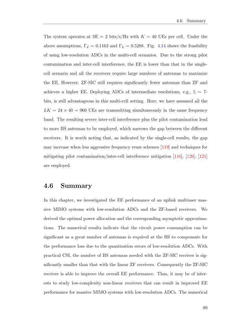
4.6. Summary
The system operates at SE = 2 bits/s/Hz with K = 40 UEs per cell. Under the
above assumptions, ΓL = 0.1163 and ΓL = 0.5288. Fig. 4.14 shows the feasibility
of using low-resolution ADCs in the multi-cell scenarios. Due to the strong pilot
contamination and inter-cell interference, the EE is lower than that in the single-
cell scenario and all the receivers require large numbers of antennas to maximize
the EE. However, ZF-SIC still requires significantly fewer antennas than ZF and
achieves a higher EE. Deploying ADCs of intermediate resolutions, e.g., 5 ∼ 7-
bits, is still advantageous in this multi-cell setting. Here, we have assumed all the
LK = 24 × 40 = 960 UEs are transmitting simultaneously in the same frequency
band. The resulting severe inter-cell interference plus the pilot contamination lead
to more BS antennas to be employed, which narrows the gap between the different
receivers. It is worth noting that, as indicated by the single-cell results, the gap
may increase when less aggressive frequency reuse schemes [119] and techniques for
mitigating pilot contamination/inter-cell interference mitigation [116], [120], [121]
are employed.
4.6 Summary
In this chapter, we investigated the EE performance of an uplink multiuser mas-
sive MIMO systems with low-resolution ADCs and the ZF-based receivers. We
derived the optimal power allocation and the corresponding asymptotic approxima-
tions. The numerical results indicate that the circuit power consumption can be
significant as a great number of antennas is required at the BS to compensate for
the performance loss due to the quantization errors of low-resolution ADCs. With
practical CSI, the number of BS antennas needed with the ZF-SIC receiver is sig-
nificantly smaller than that with the linear ZF receivers. Consequently the ZF-SIC
receiver is able to improve the overall EE performance. Thus, it may be of inter-
ests to study low-complexity non-linear receivers that can result in improved EE
performance for massive MIMO systems with low-resolution ADCs. The numerical
80
4.6. Summary
results also validated the derived closed-form approximations of the transmission
power for ZF and ZF-SIC receivers, which can account for the impairments due to
ADC quantization and imperfect channel estimation. This provides fast methods
for evaluating and optimizing the EE performance. The results show a similar trend
in a multi-cell scenario. However, the overall EE decreases for all receivers due to
the strong pilot contamination and inter-cell interference.
It should be pointed out that the present work assumes the AQNM, equal-rate
transmissions, and perfect interference cancellation. With AQNM, we have assumed
quantization noise to be independent of the desired signal, which leads to tractable
but only approximate characterization of the performance analysis. It may be in-
teresting to analyze the receivers using more accurate tools, e.g., the GMI [69].
There are also alternative transmission strategies such as the max sum-rate design
[122] that trades off efficiency and fairness by simultaneously optimizing the rate
and power allocation, which differ from the equal-rate transmissions assumed here.
When practical coding and modulation schemes are considered, decoding errors can
result in imperfect interference cancellation. These factors may also be taken into
account in future studies on massive MIMO systems with SIC receivers and low-
resolution ADCs.
81
Chapter 5
Performance Analysis of Massive MIMO
Systems With Low-Resolution ADCs Over
Rician Fading
5.1 Introduction
The EE of massive MIMO with low-resolution ADCs has been studied in the last
chapter over Rayleigh fading. This chapter investigates the SE and EE performance
of a single-cell uplink MIMO system over Rician fading channels when low-resolution
ADCs are used in both channel estimation and data detection phases. The LoS paths
in Rician fading channels make the analysis different from Rayleigh fading channels.
Assuming AQNM, we derive closed-form approximations of the SE for the MRC
and ZF receivers with CSI estimated by LMMSE channel estimation. Using the
derived approximations, we obtain the power scaling laws for both receivers. The
simulation results show that the asymptotic analysis is highly accurate under differ-
ent settings. It is found that the SE loss due to the use of low-resolution ADCs in
82
5.2. System Model
the channel estimation phase can be small when the LoS path is strong, i.e., with
a large value of K-factor, which indicates the feasibility of systems employing only
low-resolution ADCs in such applications. The ZF receivers generally outperform
the MRC receivers in SE with a realistic number of BS antennas but their gap can
be narrowed when the K-factors are increased. This is because when the LoS path
becomes strong, the inter-UE-interference mainly arise from UEs with similar an-
gles of arrival (AoA). Moreover, when the number of BS antennas goes infinite, the
non-LoS part in channel fading for UEs tends to be orthogonal, which is favorable
in terms of interference minimization. In this asymptotic case, the power-scaling
laws indicate the same SE for both receivers. Furthermore, the transmission power
can be scaled down by the number of BS antennas for a given SE while the overall
SE is limited by the resolution of ADCs. The EE of the system is also evaluated
under Rician fading by using a system-level power consumption model. The numer-
ical results show that the EE can be improved by employing ADCs with moderate
resolutions. Similar to the SE performance, the EE is higher when the LoS paths
become stronger and the ZF receiver is used.
The chapter is organized as follows. We introduce the system model in Section
5.2. The uplink SE is analyzed for the MRC and ZF receivers under perfect CSI
and the asymptotic approximations for ZF are provided in Section 5.3. The SE and
corresponding asymptotic approximation are studied for the case with imperfect CSI
in Section 5.4. The analysis is validated with numerical results in Section 5.5. The
conclusions are given in Section 5.6.
5.2 System Model
Consider the uplink of a single-cell MIMO system with M BS antennas and K
single-antenna UEs in Section 2.1. Assuming equal transmission power for all UEs,
83
5.2. System Model
the observed signals at the BS is
y =√PuHx + n =
√Pu
K∑k=1
hkxk + n, (5.1)
where y ∈ CM is the observed signal vector at the BS, x ∈ CK contains the trans-
mitted unit-power symbols xk from the K UEs, Pu is the transmission power for
all UEs and n ∈ CM is the AWGN with variance σ2 (in Joule/symbol). Following
the discussion in Section 2.2, the channel vector for UE-k over Rician fading can be
modeled as a Gaussian distribution with a non-zero mean, i.e.,
hk ∼ CN
(√KkβkKk + 1
hk,βkKk + 1
I
). (5.2)
At the BS, the received analog signals are sampled and quantized into digital
signals with finite-resolution ADCs. The quantized signal yq can be approximated
by the AQNM, which decomposes the quantizer output as the summation of the
attenuated input signal and an uncorrelated distortion, i.e.,
yq = αy + nq = α√PuHx + αn + nq, (5.3)
where nq is the additive Gaussian quantization noise which is uncorrelated with y.
The coefficient α can be calculated with (2.15). The covariance matrix of nq is
Rnq = E[nqn
Hq |H
]= α (1− α) diag
(PuHHH + σ2IM
). (5.4)
This is to approximate the quantization noise at different receiver RF chains uncor-
related, similarly to [1, 38, 123–126]. In this chapter, following [1, 38, 123–126], we
further assume that x, n and nq are Gaussian-distributed and mutually indepen-
dent. In addition, each entry in x, n and nq is with zero means and variances given
by 1, σ2 and Rnq , respectively.
84
5.3. SE With Perfect CSI
5.3 SE With Perfect CSI
At the BS, linear receiver filters are employed to estimate the transmitted signals
for recovering data. Assuming perfect CSI, the estimate of UE-k’s signal is given as
xk = gHk yq, (5.5)
where gk is the receiver filter for UE-k. Let γk denote the SINR at the BS. The
uplink gross SE Rk for UE-k is
Rk = log (1 + γk) . (5.6)
We next discuss the γk for MRC and ZF with perfect CSI.
5.3.1 SE Analysis
5.3.1.1 MRC Receiver
For the MRC receiver, the filter for UE-k is given by
gk = [H]:,k. (5.7)
The estimated signal for UE-k is written as
xk = α√Pu||hk||2xk + α
√Pu
K∑n=1,n 6=k
hHk hnxn + αhHk n + hHk nq. (5.8)
The SINR γk is computed as
γk =α2Pu‖hk‖4
Θk
, (5.9)
85
5.3. SE With Perfect CSI
where Θk denotes the distortion-plus-noise power:
Θk = α2‖hk‖2σ2 + hHk Rnqhk + α2Pu
K∑n=1,n6=k
|hHk hn|2. (5.10)
The first term on the RHS of (5.10) denotes the channel noise power while the second
term stands for the ADC quantization noise power and the last term is power of the
inter-UE interference.
5.3.1.2 ZF Receiver
ZF receivers generally outperform MRC in terms of interference suppression. When
the ZF receiver is used, the ZF filter for UE-k is
gk = [H(HHH
)−1]:,k. (5.11)
It is known that the ZF receiver is able to fully mitigate the inter-UE interference.
Thus the estimated signal in (5.8) can be further modeled by
xk = α√Puxk + αgHk n + gHk nq, (5.12)
and the SINR is
γk =α2PuΘk
, (5.13)
where Θk denotes the distortion-plus-noise power and given as
Θk = α2‖gk‖2σ2 + gHk Rnqgk. (5.14)
5.3.2 Asymptotic Analysis
In this subsection, we discuss the asymptotic analysis of the SE using random matrix
theory under the assumption of large systems. We refer to [1] treatment for the MRC
receiver and focus on the derivation for the ZF receivers in Rician fading channels.
86
5.3. SE With Perfect CSI
From (5.14), the distortion-plus-noise power Θk consists of two parts, i.e., channel
noise power α2‖gk‖2σ2 and the ADC quantization noise power gHk Rnqgk, where
‖gk‖2 =[(
HHH)−1]k,k≈ E
[(HHH
)−1]k,k, (5.15)
where the expectation is w.r.t. the small-scale fading. From [23, Theorem 4], HHH
follows a non-central Wishart distribution and the squared Euclidean norm of UE-k’s
filter satisfies
‖gk‖2 ≈[Σ−1]k,k
βk (M −K)(5.16)
where
Σ , (Ω + IK)−1 +1
M
[Ω (Ω + IK)−1]1/2 HHH
[Ω (Ω + IK)−1]1/2 . (5.17)
For the quantization noise, the following approximation tends to be accurate in a
large system,
gHk Rnqgk ≈ gHk E[Rnq
]gk, (5.18)
where the expectation is w.r.t. the small-scale fading. From (2.6) and (2.8),
E[|Hm,k|2] =KkKk + 1
+1
Kk + 1= 1. (5.19)
With (5.19), we can approximate (5.4) by
E[Rnq
]≈ α (1− α)
(Pu
K∑k=1
βk + σ2
)IM . (5.20)
Substituting (5.16) and (5.20) into (5.18), the power of the quantization noise can
be approximated as
gHk Rnqgk ≈ α (1− α)
(Pu
K∑k=1
βk + σ2
)[Σ−1]k,k
βk (M −K). (5.21)
87
5.4. SE With Imperfect CSI
Finally, substituting (5.16) and (5.21) into (5.14), we can find the distortion-plus-
noise power for the ZF receiver and approximate the SINR in (5.13) by
γk ≈Puβk (M −K)(
1ασ2 +
(1α− 1)Pu
K∑n=1
βn
)[Σ−1]k,k
(5.22)
This can be used to predict the SE performance along with (5.6).
5.4 SE With Imperfect CSI
In practice, the CSI is often obtained during a training phase. In this chapter, we
consider the LMMSE channel estimation. Following [1, 23, 38, 127] we assume that
the large-scale fading coefficient, the deterministic component H and Ω are known
at the BS.
5.4.1 LMMSE Channel Estimation
In the training phase, each UE transmits a pilot signal of length L to the BS and
the pilot signals for all UEs can be denoted by a K × L matrix Φ, where Φ =
[φ1,φ2, · · · ,φK ]T ∈ CK×L. The received signals, Yt ∈ CM×L, at the BS are given
by
Yt =√PtHΦ + Nt (5.23)
and the quantized received signals can be modeled by AQNM as
Ytq = α
√PtHΦ + αNt + Nt
q, (5.24)
where Pt is the pilot transmission power which is assumed to be the same as Pu in the
data transmission phase for all the UEs. The channel noise and ADC quantization
noise are denoted by Nt and Ntq, respectively. Let Hw , Hwdiag
√β1, · · · ,
√βK
and assume orthogonal training signals with ΦΦH , LIK [23]. After removing the
88
5.4. SE With Imperfect CSI
LoS part which is assumed known at the BS, (5.24) can be simplified to
Ytq =α
√PuHw
[(Ω + IK)−1]1/2 Φ + αNt + Nt
q (5.25)
For the l-th pilot symbol,
ytql = α√Pu
K∑k=1
hw,kφk,l (Kk + 1)−1/2 + αntl + ntq,l. (5.26)
and
Rtnq = α (1− α) diag
(Rytl
)(5.27)
where
Rytl= E
[ytly
tHl
](5.28)
and
Rtnq = α (1− α)
(σ2 + Pu
K∑n=1
βn
)IM . (5.29)
Now let us consider the LMMSE estimation of UE-k’s channel hk. Let xk denote
the k-th row of X where X ,√PuΦ and ytk , Yt
qxHk . We have
ytk = αHw
[(Ω + IK)−1]1/2 XxHk + αNtxHk + Nt
qxHk
= αLPuhw,k (Kk + 1)−1/2 + αNtxHk + Ntqx
Hk .
(5.30)
For each UE-k, assume that the channel vector hw,k follows i.i.d. zero-mean Gaussian
distribution with variance βk. The LMMSE estimate of hw,k is then computed as,
hw,k = ψkytk, (5.31)
where
ψk = Chw,k,ytkR−1
ytk(5.32)
89
5.4. SE With Imperfect CSI
and Chw,k,ytk
is the covariance matrix of hw,k and ytk, which can be calculated by
Chw,k,ytk
= αPuLβk (Kk + 1)−1/2 IM . (5.33)
Rytkis the variance matrix of ytk and
Rytk= α2L2βkP
2u (Kk + 1)−1 IM + α2σ2LPuIM + LPuα (1− α)
(σ2 + Pu
K∑n=1
βn
)IM .
Now the channel estimator for UE-k in (5.32) can be written as
ψk =βk (Kk + 1)−1/2
αLβkPu (Kk + 1)−1 + σ2 + (1− α)PuK∑n=1
βn
.(5.34)
Recall that the deterministic component H and Ω are known at the BS. The channel
estimation error for UE-k
ek , hk − hk =1√Kk + 1
(hw,k − hw,k
).
It can be shown that the variance of the entries in ek can be computed as
σ2ek
=βk (1− ξk)Kk + 1
(5.35)
where
ξk =PuLβk
PuLβk + (Kk + 1)
[σ2
α+(
1α− 1)Pu
K∑n=1
βn
] .(5.36)
Correspondingly, the variance of the estimate of the non-LoS component of the
channel for UE-k is
σ2k =
βkξkKk + 1
. (5.37)
90
5.4. SE With Imperfect CSI
5.4.2 SE Analysis
The data transmission phase follows the training phase. Let γk denote the SINR
with imperfect CSI. The uplink SE is given by
Rk = log (1 + γk) . (5.38)
We now discuss γk for the MRC and ZF receivers with imperfect CSI.
5.4.2.1 MRC Receiver
When the MRC receiver is used, the filter for UE-k
gk = [H]:,k. (5.39)
The SINR γk is given by
γk =α2Pu‖hk‖4
Θk
, (5.40)
where Θk denotes the distortion-plus-noise power
Θk =α2‖hk‖2σ2 + hHk Rnq hk + α2Pu
K∑n=1,n6=k
|hHk hn|2 + α2Pu
K∑n=1
‖hk‖2σ2en , (5.41)
which consists of contributions from the channel noise, ADC quantization noise,
inter-UE interference and channel estimation error.
5.4.2.2 ZF Receiver
When the ZF receiver is used,
gk = [H(HHH
)−1
]:,k. (5.42)
91
5.4. SE With Imperfect CSI
Similar to the case with perfect CSI, the SINR γk with ZF receivers is given as
γk =α2Pu
Θk
, (5.43)
where
Θk = α2‖gk‖2σ2 + gHk Rnq gk + α2Pu
K∑n=1
||gk||2σ2en . (5.44)
In particular, the covariance matrix of quantization noise, Rnq , in (5.41) and (5.44)
is defined in (5.4). Note also that in contrast to the case with perfect CSI, the ZF
receiver cannot fully mitigate the inter-UE interference, as seen from the last item
of (5.44).
5.4.3 Asymptotic Analysis
We next derive asymptotic approximations of the SINR for the MRC and ZF re-
ceivers with imperfect CSI, which can provide insights about the influence of the
K-factor, ADC resolution, and number of BS antennas on the SE. From the analysis
in Section 5.4.1, the estimated Rayleigh fading channel vectors for different UEs hw
are mutually independent and the entries can be modeled as i.i.d. random variables
(RVs) for a given UE. For UE-k, the entries of hw,k can be modeled by
Hw,mk ∼ CN (0, βkξk),
where ξk is given in (5.36). Let
Hmk =
√KkβkKk + 1
ρmk +
√1
Kk + 1δmk, (5.45)
where following (2.8)
ρmk , e−j(m−1)π sin(θk) = ρcmk − jρsmk
92
5.4. SE With Imperfect CSI
and
δmk , δcmk + jδsmk
with zero mean and variance of βkξk2
for independent real and imaginary parts δcmk
and δsmk. In the following, we assume large systems and derive asymptotic approxi-
mations of the SE.
5.4.3.1 MRC Receiver
In order to find the asymptotic approximation to (5.40) for the MRC receiver, the
approximation expressions of ‖hk‖2, ‖hk‖4 and |hHk hn|2 are needed. As derived in
the Appendix, when M →∞,
‖hk‖2 ≈ Mβk (Kk + ξk)
Kk + 1, (5.46)
‖hk‖4 ≈ Mβ2k (2Kkξk + 2MKkξk +MK2
k + (M + 1) ξ2k)
(Kk + 1)2 , (5.47)
and
|hHk hn|2 ≈βnβk (KkKnλ2
kn +MKkξn +MKnξk +Mξnξk)
(Kk + 1) (Kn + 1). (5.48)
The SINR γk of the system for the MRC receiver can then be approximated by
γk ≈α2Pu
Mβ2k
(Kk+1)2 (2Kkξk + 2MKkξk +MK2k + (M + 1) ξ2
k)
Θk
, (5.49)
where Θk is given as
93
5.4. SE With Imperfect CSI
Θk , α2‖hk‖2σ2 + hHk Rnq hk + α2Pu
K∑n=1,n6=k
|hHk hn|2 + α2Pu
K∑n=1
‖hHk ‖2σ2en
≈Mβk
(Kk + ξk
)Kk + 1
(ασ2 + α (1− α)Pu
K∑k=1
βk + α2Pu
K∑n=1
σ2en
)
+ α2Pu
K∑n=1,n 6=k
βnβk(Kk + 1) (Kn + 1)
(KkKnλ2kn +MKkξn +MKnξk +Mξnξk).
(5.50)
5.4.3.2 ZF Receiver
It is known that when M is large, for the ZF filter for UE-k,
‖gk‖2 =
[(HHH
)−1]k,k
≈ E[(
HHH)−1]k,k
. (5.51)
Similarly to the case with perfect CSI, HHH follows a non-central Wishart distri-
bution. Using a similar strategy as [23, (53), (54)], we can obtain
‖gk‖2 ≈
[Σ−1
]k,k
βk (M −K), (5.52)
where
Σ , Ξ (Ω + IK)−1 +1
M
[Ω (Ω + IK)−1]1/2 HHH
[Ω (Ω + IK)−1]1/2 , (5.53)
and Ξ is a K ×K diagonal matrix with Ξk,k = ξk. As such the SINR
γk =α2Pu
Θk
(5.54)
for the ZF receivers can be approximated by using
Θk ≈
[ασ2 + α (1− α)Pu
K∑n=1
βn + α2PuK∑i=1
σ2ei
] [Σ−1
]k,k
βk (M −K). (5.55)
94
5.4. SE With Imperfect CSI
5.4.4 Power-Scaling Laws and Influence of ADC Resolution
5.4.4.1 MRC Receivers
The asymptotic approximations derived above allow the study of the power scaling
law for MRC receivers with imperfect CSI, which provides insight on the performance
when the number of antennas increases. Consider the scenario M → ∞. Multiply
1M2 to the numerator and denominator of (5.40) and let Pu = Eu
Mν , where ν > 0 and
Eu is a fixed value. We have
α2 EuMν+2
|hHk hi|2 = α2 EuMν| 1
MhHk hi|2
a.s.→ 0. (5.56)
Following (5.56), removing the relevant zero items in (5.40), it then reduces to
γk =EuMν ‖hk‖2
σ2
α+ Eu
Mν
K∑n=1
βn
(1−αα
+ 1−ξnKn+1
) . (5.57)
Considering αEuσ2Mν ‖hk‖2 = αEu
σ2Mν−1 | 1M
hHk hk| and following the approximation of ‖hk‖2
in (5.46), the SINR tends to be
γkM→∞→ αEu
σ2Mν−1
∣∣∣∣ 1
MhHk hk
∣∣∣∣≈ αEuσ2Mν−1
(KkβkKk + 1
+ξkβkKk + 1
)=
αKkβkEuσ2Mν−1 (Kk + 1)
+αE2
uβ2kL
σ2M2ν−1 (Kk + 1)
(L EuMν + σ2
α+ ( 1
α− 1) Eu
Mν
K∑n=1
βn
) .(5.58)
It is easy to observe that when M →∞, the SINR
γk =αKkβkEu
σ2Mν−1 (Kk + 1)+
αE2uβ
2kL
M2ν−1 (Kk + 1) σ4
α
. (5.59)
The power scaling law for the MRC receiver can now be discussed from (5.59).
When the system operates in Rayleigh fading channels, i.e., Kk = 0, the SINR
95
5.4. SE With Imperfect CSI
tends to be a constant value
γk,mrc =α2E2
uβ2kL
σ4(5.60)
if ν = 0.5. This shows that under Rayleigh fading, the transmission power can be
scaled by the square root of the number of BS antennas. From (5.60), when low-
resolution ADCs are used for both the channel estimation and data transmission
phases, the SINR decreases quadratically with α which characterizes the quantiza-
tion error. This differs from [1, (24)], which shows the SINR decreases linearly with
α when ideal ADCs are used (in a round-robin manner) for the LMMSE channel
estimation.
For Rician fading channels, i.e., Kk 6= 0, the SINR tends to be a constant value
γk,mrc =αKkβkEuσ2 (Kk + 1)
(5.61)
if ν = 1. This suggests that in Rician fading channels, the transmission power can
be scaled linearly by the number of BS antennas when the SE is fixed. In contrast
to the case of Rayleigh fading, the SE loss caused by the usage of low-resolution
ADCs for channel estimation diminishes when M → ∞, and the asymptotic SINR
becomes the same as [1, (25)] which assumes ideal ADCs for channel estimation.
5.4.4.2 ZF Receivers
We next derive the power scaling law for the ZF receivers under imperfect CSI,
following the same treatments as for the MRC receivers. Assuming M → ∞ and
removing the zero items when M →∞, (5.43) then becomes
γk ≈Eu
1αMν‖gk‖2σ2
. (5.62)
From [23, Corollary 5], when M is large, 1M
HHH becomes an identity matrix.
Following this, substituting the k-th diagonal entry in (5.53) into (5.52), (5.62) can
96
5.4. SE With Imperfect CSI
be written as
Eu1αMν‖gk‖2σ2
=Eu (M −K)
1αMνσ2
KkβkKk + 1
+ξkβkKk + 1
=αEu
(1− K
M
)Mν−1σ2
KkβkKk + 1
+ξkβkKk + 1
=
αEuKkβk(Kk + 1)Mν−1σ2
+αEuβk
EuMνLβk
(Kk + 1)Mν−1σ2
(EuMνLβk + σ2
α+(
1α− 1)EuMν
K∑n=1
βn
)=
αEuKkβk(Kk + 1)Mν−1σ2
+Lα2E2
uβ2k
(Kk + 1)M2ν−1σ4.
(5.63)
For Rayleigh fading channels, i.e., Kk = 0, the SINR tends to be
γk,zf =α2E2
uβ2kL
σ4(5.64)
when ν = 0.5. For Rician fading channels, i.e., Kk 6= 0, the SINR tends to be
γk,zf =αKkβkEuσ2 (Kk + 1)
(5.65)
when ν = 1. Therefore, for a given SE, the transmission power can be scaled by M
for Rician fading and by√M for Rayleigh fading, where M is the number of BS
antennas. It is observed that the ZF and MRC receivers have the same asymptotic
expressions of the SINR when M →∞. This is reasonable as using a large number
of antennas the MRC and ZF receivers exhibit similar performance due to channel
hardening [24] where the channels of different UEs become orthogonal to each other.
It can be observed from the above asymptotic analysis that, for both receivers,
the SE loss due to the use of low-resolution ADCs in channel estimation may be
lower if strong LoS paths are present, which encourages the usage of low-resolution
ADCs in some practical scenarios such as small cells and UAV transmissions. In fact,
it can be verified from (5.37) that as the K-factor increases, the channel estimation
error caused by ADC quantization noise diminishes and γk improves.
97
5.5. Numerical Results
5.4.5 Very Strong LoS Paths
We next consider scenarios where the channels have very strong LoS paths. For
simplicity, assume that all UEs have the same value of K-factors, i.e., Ki = Kk,∀i,
and Kk →∞. For the MRC receiver, (5.49) tends to
γk =PuM
2βk
M
(σ2
α+ 1−α
αPu
K∑n=1
βn
)+ Pu
K∑n=1,n 6=k
βnλ2kn
. (5.66)
This indicates that when the LoS paths become strong, only the UEs with similar
AoAs lead to inter-UE-interference. It is also observed that the overall SE perfor-
mances is limited by the resolution of ADCs.
For the ZF receiver, (5.54) tends to
γk ≈βkPu (M −K)[
σ2
α+(
1−αα
)Pu
N∑n=1
βn
] [(1M
HHH)−1]k,k.
(5.67)
Similar to the MRC receiver, the effects of using low-resolution ADCs in channel
estimation phase diminishes with a strong LoS path and the overall SE is limited
by the resolution of ADCs.
5.5 Numerical Results
We now present numerical results to validate the analysis in Section IV. We consider
a single-cell, uplink system with K = 10 UEs. The large-scale fading coefficients
βk are set the same as [38]. The K-factors for all UEs are assumed the same,
following [38], [23]. The same low-resolution ADCs are adopted for the channel
estimation and data transmission phases. The pilot length for each UE is fixed to
L = K except for Fig. 5.3. The AoAs of different UEs are generated randomly and
the average SE is measured.
Fig. 5.1 shows the SE performance under different values of transmission power,
98
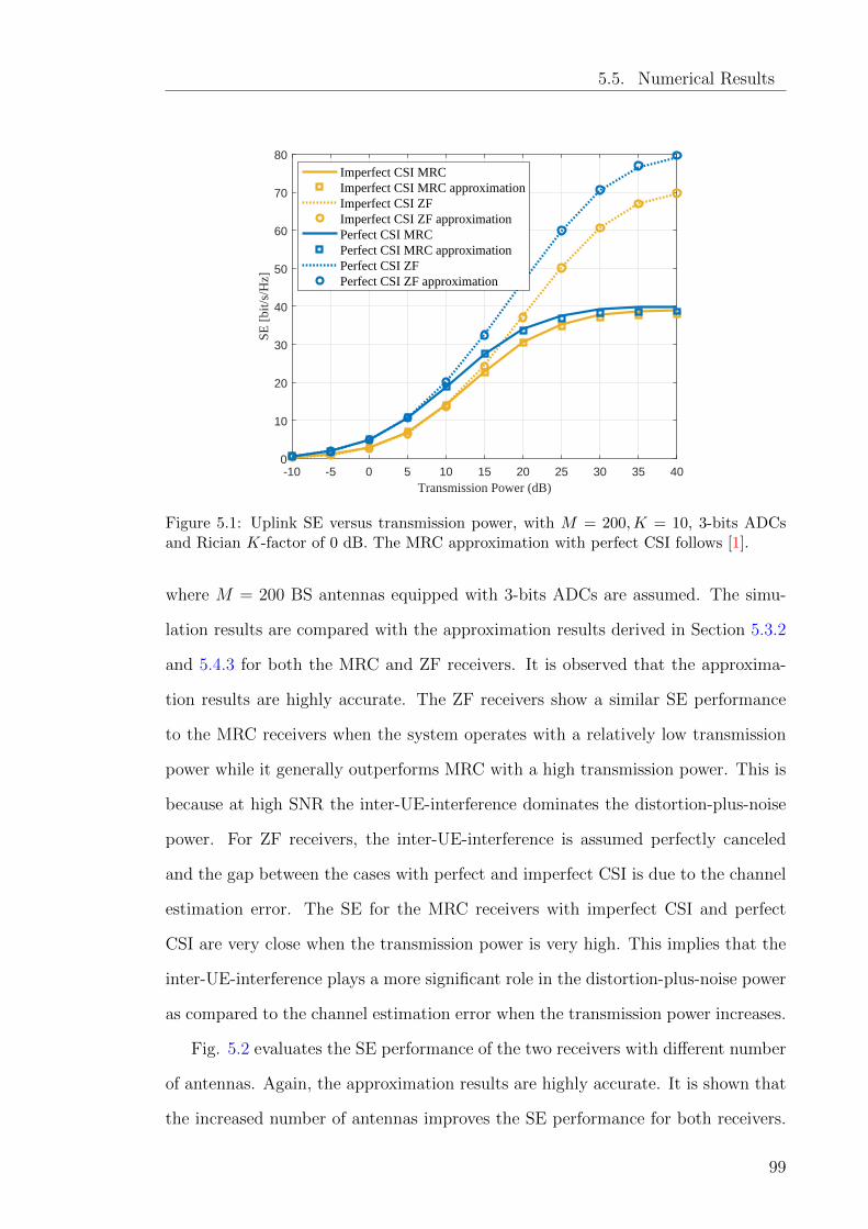
5.5. Numerical Results
-10 -5 0 5 10 15 20 25 30 35 40Transmission Power (dB)
0
10
20
30
40
50
60
70
80
SE [
bit/s
/Hz]
Imperfect CSI MRCImperfect CSI MRC approximationImperfect CSI ZFImperfect CSI ZF approximationPerfect CSI MRCPerfect CSI MRC approximationPerfect CSI ZFPerfect CSI ZF approximation
Figure 5.1: Uplink SE versus transmission power, with M = 200,K = 10, 3-bits ADCsand Rician K-factor of 0 dB. The MRC approximation with perfect CSI follows [1].
where M = 200 BS antennas equipped with 3-bits ADCs are assumed. The simu-
lation results are compared with the approximation results derived in Section 5.3.2
and 5.4.3 for both the MRC and ZF receivers. It is observed that the approxima-
tion results are highly accurate. The ZF receivers show a similar SE performance
to the MRC receivers when the system operates with a relatively low transmission
power while it generally outperforms MRC with a high transmission power. This is
because at high SNR the inter-UE-interference dominates the distortion-plus-noise
power. For ZF receivers, the inter-UE-interference is assumed perfectly canceled
and the gap between the cases with perfect and imperfect CSI is due to the channel
estimation error. The SE for the MRC receivers with imperfect CSI and perfect
CSI are very close when the transmission power is very high. This implies that the
inter-UE-interference plays a more significant role in the distortion-plus-noise power
as compared to the channel estimation error when the transmission power increases.
Fig. 5.2 evaluates the SE performance of the two receivers with different number
of antennas. Again, the approximation results are highly accurate. It is shown that
the increased number of antennas improves the SE performance for both receivers.
99
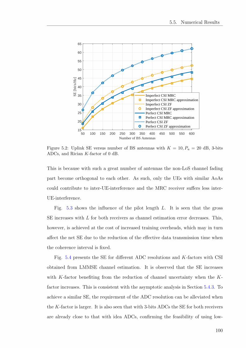
5.5. Numerical Results
50 100 150 200 250 300 350 400 450 500 550 600Number of BS Antennas
15
20
25
30
35
40
45
50
55
60
65
SE [
bit/s
/Hz]
Imperfect CSI MRCImperfect CSI MRC approximationImperfect CSI ZFImperfect CSI ZF approximationPerfect CSI MRCPerfect CSI MRC approximationPerfect CSI ZFPerfect CSI ZF approximation
Figure 5.2: Uplink SE versus number of BS antennas with K = 10, Pu = 20 dB, 3-bitsADCs, and Rician K-factor of 0 dB.
This is because with such a great number of antennas the non-LoS channel fading
part become orthogonal to each other. As such, only the UEs with similar AoAs
could contribute to inter-UE-interference and the MRC receiver suffers less inter-
UE-interference.
Fig. 5.3 shows the influence of the pilot length L. It is seen that the gross
SE increases with L for both receivers as channel estimation error decreases. This,
however, is achieved at the cost of increased training overheads, which may in turn
affect the net SE due to the reduction of the effective data transmission time when
the coherence interval is fixed.
Fig. 5.4 presents the SE for different ADC resolutions and K-factors with CSI
obtained from LMMSE channel estimation. It is observed that the SE increases
with K-factor benefiting from the reduction of channel uncertainty when the K-
factor increases. This is consistent with the asymptotic analysis in Section 5.4.3. To
achieve a similar SE, the requirement of the ADC resolution can be alleviated when
the K-factor is larger. It is also seen that with 3-bits ADCs the SE for both receivers
are already close to that with idea ADCs, confirming the feasibility of using low-
100
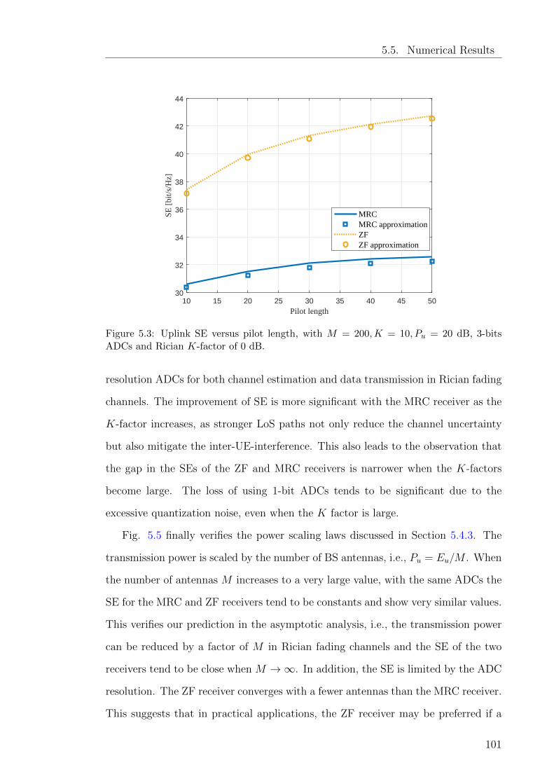
5.5. Numerical Results
10 15 20 25 30 35 40 45 50Pilot length
30
32
34
36
38
40
42
44
SE [
bit/s
/Hz]
MRCMRC approximationZFZF approximation
Figure 5.3: Uplink SE versus pilot length, with M = 200,K = 10, Pu = 20 dB, 3-bitsADCs and Rician K-factor of 0 dB.
resolution ADCs for both channel estimation and data transmission in Rician fading
channels. The improvement of SE is more significant with the MRC receiver as the
K-factor increases, as stronger LoS paths not only reduce the channel uncertainty
but also mitigate the inter-UE-interference. This also leads to the observation that
the gap in the SEs of the ZF and MRC receivers is narrower when the K-factors
become large. The loss of using 1-bit ADCs tends to be significant due to the
excessive quantization noise, even when the K factor is large.
Fig. 5.5 finally verifies the power scaling laws discussed in Section 5.4.3. The
transmission power is scaled by the number of BS antennas, i.e., Pu = Eu/M . When
the number of antennas M increases to a very large value, with the same ADCs the
SE for the MRC and ZF receivers tend to be constants and show very similar values.
This verifies our prediction in the asymptotic analysis, i.e., the transmission power
can be reduced by a factor of M in Rician fading channels and the SE of the two
receivers tend to be close when M →∞. In addition, the SE is limited by the ADC
resolution. The ZF receiver converges with a fewer antennas than the MRC receiver.
This suggests that in practical applications, the ZF receiver may be preferred if a
101
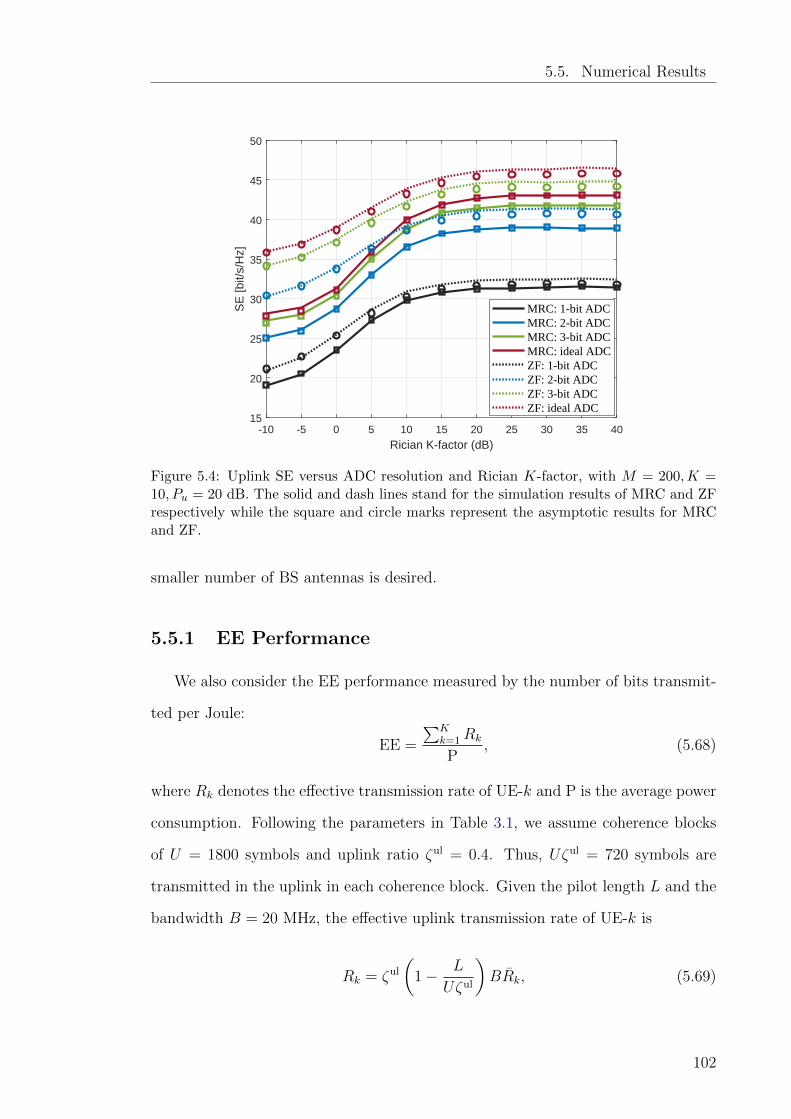
5.5. Numerical Results
-10 -5 0 5 10 15 20 25 30 35 40
Rician K-factor (dB)
15
20
25
30
35
40
45
50
SE
[bit/
s/H
z]
MRC: 1-bit ADCMRC: 2-bit ADCMRC: 3-bit ADCMRC: ideal ADCZF: 1-bit ADCZF: 2-bit ADCZF: 3-bit ADCZF: ideal ADC
Figure 5.4: Uplink SE versus ADC resolution and Rician K-factor, with M = 200,K =10, Pu = 20 dB. The solid and dash lines stand for the simulation results of MRC and ZFrespectively while the square and circle marks represent the asymptotic results for MRCand ZF.
smaller number of BS antennas is desired.
5.5.1 EE Performance
We also consider the EE performance measured by the number of bits transmit-
ted per Joule:
EE =
∑Kk=1Rk
P, (5.68)
where Rk denotes the effective transmission rate of UE-k and P is the average power
consumption. Following the parameters in Table 3.1, we assume coherence blocks
of U = 1800 symbols and uplink ratio ζul = 0.4. Thus, Uζul = 720 symbols are
transmitted in the uplink in each coherence block. Given the pilot length L and the
bandwidth B = 20 MHz, the effective uplink transmission rate of UE-k is
Rk = ζul
(1− L
Uζul
)BRk, (5.69)
102
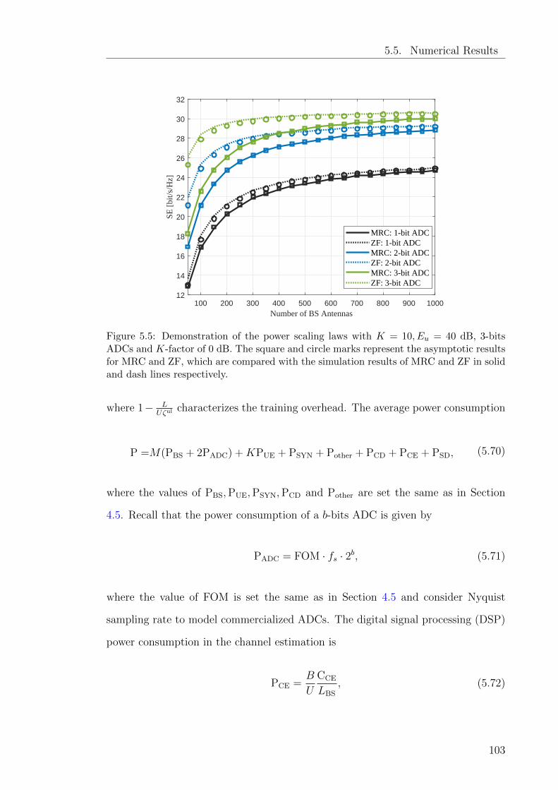
5.5. Numerical Results
100 200 300 400 500 600 700 800 900 1000Number of BS Antennas
12
14
16
18
20
22
24
26
28
30
32
SE [
bit/s
/Hz]
MRC: 1-bit ADCZF: 1-bit ADCMRC: 2-bit ADCZF: 2-bit ADCMRC: 3-bit ADCZF: 3-bit ADC
Figure 5.5: Demonstration of the power scaling laws with K = 10, Eu = 40 dB, 3-bitsADCs and K-factor of 0 dB. The square and circle marks represent the asymptotic resultsfor MRC and ZF, which are compared with the simulation results of MRC and ZF in solidand dash lines respectively.
where 1− LUζul characterizes the training overhead. The average power consumption
P =M(PBS + 2PADC) +KPUE + PSYN + Pother + PCD + PCE + PSD, (5.70)
where the values of PBS,PUE,PSYN,PCD and Pother are set the same as in Section
4.5. Recall that the power consumption of a b-bits ADC is given by
PADC = FOM · fs · 2b, (5.71)
where the value of FOM is set the same as in Section 4.5 and consider Nyquist
sampling rate to model commercialized ADCs. The digital signal processing (DSP)
power consumption in the channel estimation is
PCE =B
U
CCE
LBS
, (5.72)
103
5.5. Numerical Results
where the value of LBS can be founded in Table 3.1 and the computational complexity
for estimating the K UEs’ channels is approximately CCE = 2LKM + 2K2 + MK
flops. We also take into account the power consumed by signal detection:
PSD = Bζul
(1− Kτul
ζulU
)Csymbol
LBS+ PBL, (5.73)
where Csymbol is the complexity of recovering a symbol:
Csymbol = 2KM −K flops (5.74)
for both receivers. The computational power consumed due to the filter calculation,
PBL, is given as
PBL =BCwm
ULBS
, (5.75)
where Cwm is the complexity involved in obtaining the filters. Specifically, for ZF
receivers Cwm = 13K3 + 3K2M + KM − 1
3K flops. For MRC receivers, as shown
in (5.7) and (5.39), the filters are directly obtained from the channel matrix. Thus,
the complexity for finding the MRC filter is ignored.
Fig. 5.6 shows the achievable EE of the system with different numbers of BS
antennas over Rician fading. It is shown that the EE is not monotone with the
number of antennas and can be lower with a large number of antennas, e.g., M =
200, than that with a moderate number of antennas, e.g., M = 80. This is due to
the significant RF circuit power consumption for a large system.
Fig. 5.7 shows the achievable EE with different resolutions of ADCs as well as
different values of the Rician K-factors for the MRC and ZF receivers. The EE
performance is higher for both receivers when the LoS paths are stronger (i.e., with
a larger Rician-K factor). Moreover, ADCs with a moderate resolution, e.g., 5-bits,
achieve higher EE than that with high-resolution or extremely low-resolution ADCs.
It is also observed that the ZF receivers generally outperform the MRC receivers.
This indicates that although MRC receivers require lower computational complexity
104
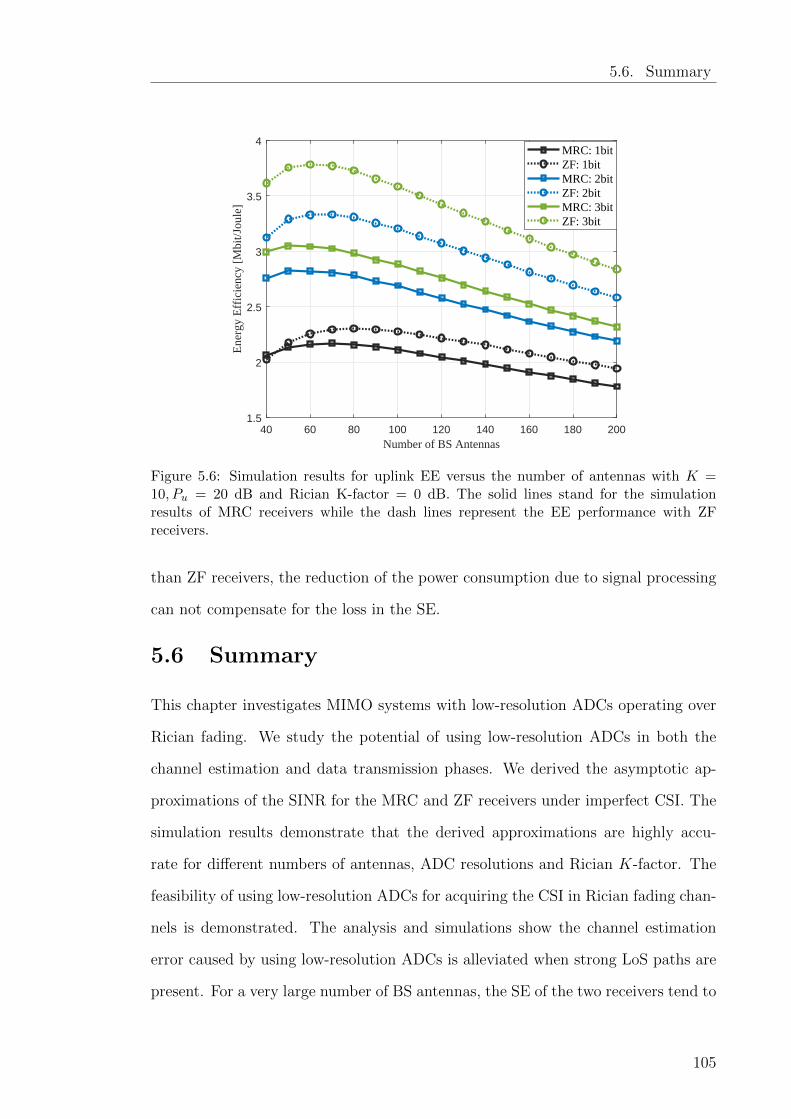
5.6. Summary
40 60 80 100 120 140 160 180 200Number of BS Antennas
1.5
2
2.5
3
3.5
4
Ene
rgy
Eff
icie
ncy
[Mbi
t/Jou
le]
MRC: 1bitZF: 1bitMRC: 2bitZF: 2bitMRC: 3bitZF: 3bit
Figure 5.6: Simulation results for uplink EE versus the number of antennas with K =10, Pu = 20 dB and Rician K-factor = 0 dB. The solid lines stand for the simulationresults of MRC receivers while the dash lines represent the EE performance with ZFreceivers.
than ZF receivers, the reduction of the power consumption due to signal processing
can not compensate for the loss in the SE.
5.6 Summary
This chapter investigates MIMO systems with low-resolution ADCs operating over
Rician fading. We study the potential of using low-resolution ADCs in both the
channel estimation and data transmission phases. We derived the asymptotic ap-
proximations of the SINR for the MRC and ZF receivers under imperfect CSI. The
simulation results demonstrate that the derived approximations are highly accu-
rate for different numbers of antennas, ADC resolutions and Rician K-factor. The
feasibility of using low-resolution ADCs for acquiring the CSI in Rician fading chan-
nels is demonstrated. The analysis and simulations show the channel estimation
error caused by using low-resolution ADCs is alleviated when strong LoS paths are
present. For a very large number of BS antennas, the SE of the two receivers tend to
105
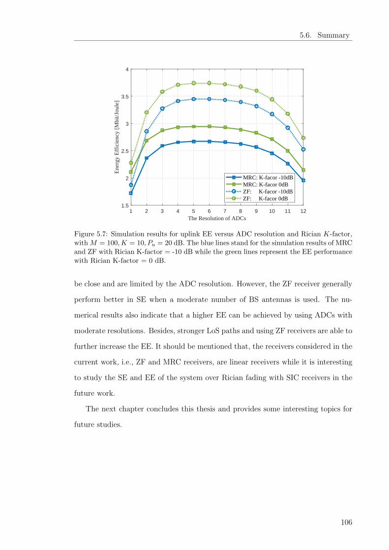
5.6. Summary
1 2 3 4 5 6 7 8 9 10 11 12The Resolution of ADCs
1.5
2
2.5
3
3.5
4
Ene
rgy
Eff
icie
ncy
[Mbi
t/Jou
le]
MRC: K-facor -10dBMRC: K-facor 0dBZF: K-facor -10dBZF: K-facor 0dB
Figure 5.7: Simulation results for uplink EE versus ADC resolution and Rician K-factor,with M = 100,K = 10, Pu = 20 dB. The blue lines stand for the simulation results of MRCand ZF with Rician K-factor = -10 dB while the green lines represent the EE performancewith Rician K-factor = 0 dB.
be close and are limited by the ADC resolution. However, the ZF receiver generally
perform better in SE when a moderate number of BS antennas is used. The nu-
merical results also indicate that a higher EE can be achieved by using ADCs with
moderate resolutions. Besides, stronger LoS paths and using ZF receivers are able to
further increase the EE. It should be mentioned that, the receivers considered in the
current work, i.e., ZF and MRC receivers, are linear receivers while it is interesting
to study the SE and EE of the system over Rician fading with SIC receivers in the
future work.
The next chapter concludes this thesis and provides some interesting topics for
future studies.
106
Chapter 6
Conclusion
The thesis conducts a study on the EE and SE of massive MIMO systems as pre-
sented in the last three chapters. This chapter briefly summaries the contributions
and lists some potential topics for future research.
6.1 Summary of the Contributions
The main contributions in this thesis are briefly summarized as follows:
• We investigate the EE when nonlinear SIC receivers are employed at the BSs.
We show that to achieve the same QoS, the SIC receivers require fewer anten-
nas at BSs, but only moderate increase of the receiver complexity. As a result,
the EE with the SIC receivers can be significantly higher than that with linear
receivers, as demonstrated by the numerical results.
• The influence of signal detection schemes on the EE of uplink MIMO systems
with low-resolution ADCs has been studied in both single cell and multi-
cell scenarios. The asymptotic analysis and numerical results indicate that
the number of BS antennas needed with the ZF-SIC receivers is significantly
smaller than that with the ZF receivers. Meanwhile, the increase of power
consumption of signal processing with ZF-SIC can be moderate, due to the fact
107
6.2. Future Research
that the receiver weights are reused in a coherent block and the dimensionality
is reduced. Consequently, the ZF-SIC receiver is able to improve the overall
EE for massive MIMO systems with practical ADCs.
• MRC and ZF receivers are considered under the assumption of perfect and
imperfect CSI over Rician fading channel. It is shown that a large value
of K-factors could lead to better EE and SE performance and alleviate the
influence of quantization noise on channel estimation. Moreover, the power
scaling laws derived for both receivers under imperfect CSI show that when
the number of BS antennas is very large, without loss of SE performance,
the transmission power can be scaled by the number of BS antennas while
the overall performance is limited by the resolution of ADCs. Besides, it is
also shown that higher EE can be achieved by using the ADCs with moderate
resolutions and stronger LoS paths and using ZF receivers are able to further
increase the EE.
6.2 Future Research
Some extensions from this thesis, which could be interesting for future work, are
listed below:
• Pilot contamination: pilot contamination is known as one of the significant
limitations for massive MIMO systems. The performance degradation caused
by interference from other cells during the channel estimation can not be easily
solved by increasing the number of antennas. In Chapter 4, we have made
a brief study of the EE performance when pilot contamination exists. The
design of the cell-size, the receivers and the frequency-reuse factors during the
training phase are still open topics.
• Downlink transmission: The EE of uplink massive MIMO systems has been
studied in this thesis. In [10], the hardware and signal processing has been
108
6.2. Future Research
jointly considered to optimize the EE performance of massive MIMO system in
downlink transmission. The corresponding EE performance of low complexity
non-linear precoders, e.g., Tomlinson-Harashima precoder (THP) etc. [128–
130], have been rarely studied and could be interesting in the future work.
• Oversampling: The performance of low-resolution ADCs with Nyquist sam-
pling rate has been studied in Chapter 4 and 5. As mentioned in Section
2.4.2.1, oversampling is widely considered in the industry as it can improve
the performance of ADCs. Recently, the SE performance of massive MIMO
systems with oversampling ADCs is studied [131–133]. However, the joint op-
timizations of the BS antennas, the resolution of ADCs and the oversampling
factors with different receivers from the EE perspective are still open topics.
• Millimeter wave: This thesis focuses on the EE of massive MIMO over con-
ventional sub-6G Hz frequencies. Thanks to the great available bandwidth,
millimeter wave (mmWave), which is in the range of 30-300 GHz, can pro-
vide high data rate [134] and has been considered as a promising technology
for future wireless communication. In outdoor transmission, massive MIMO
systems are considered to be ideal for mmWave in long-range communication
[135–143]. Although there are some related works [135, 137, 140] that study
the EE of massive MIMO system in mmWave, the joint consideration of RF
hardware and signal processing to improve EE is still an open area.
109
Appendix A
Appendix
In order to find the asymptotic approximation to (5.40) for the MRC receiver, let
us analyze ‖hk‖2, ‖hk‖4 and |hHk hn|2.
We start with ‖hk‖2. As M →∞,
‖hk‖2 ≈M∑m=1
E(|Hmk|2
).
From (5.45),
‖hk‖2 ≈
M∑m=1
E(Kkβk|ρmk|2 + 2
√KkβkR(ρ∗mkδmk) + |δmk|2
)Kk + 1
.(A.1)
Noticing that |ρmk|2 = 1, E(|δmk|2) = βkξk, and E(δmk) = 0, we have
‖hk‖2 ≈ 1
Kk + 1
M∑m=1
E (Kkβk + βkξk)
=Mβk (Kk + ξk)
Kk + 1.
(A.2)
We next study
110
‖hk‖4 ≈[ M∑m=1
E(|Hmk|2
)]2
=1
(Kk + 1)2
M∑m=1
E[Kkβk|ρmk|2 +
√Kkβk(ρ∗mkδmk + ρmkδ
∗mk) + |δmk|2
]2
=1
(Kk + 1)2E[( M∑
m=1
Kkβk|ρmk|2)2
+
(M∑m=1
Kkβkρ∗mkδmk
)2
+
(M∑m=1
Kkβkρmkδ∗mk
)2
+
( M∑m=1
|δmk|2)2
+ 2M∑m=1
Kkβk (ρ∗mkδmk)2 + 2
M∑m1=1
M∑m2=1
Kkβk|ρm1k|2|δm2,k|2]
(A.3)
Invoking the assumptions in (5.45) and after some mathematical manipulations we
have
‖hk‖4 ≈ 2MKkβkβk + 2M2Kkβkβk + (MKkβk)2 + (M2 +M) β2k
(Kk + 1)2 .(A.4)
After some simplifications, we find (5.47).
We finally consider
|hHk hn|2 ≈
∣∣∣∣∣M∑m=1
E(H∗mkHmn
)∣∣∣∣∣2
=1
(Kk + 1) (Kn + 1)
∣∣∣∣( M∑m=1
E√KkβkKnβnρ∗mkρmn
+√Kkβkρ∗mkδmn +
√Knβnρmnδ∗mk + δ∗mkδmn
)∣∣∣∣2(A.5)
Following the analysis in Section 5.4.3, δmk is independent of δmn for ∀n 6= k and
E(δmk) = 0. Removing the zero items, the remaining items in (A.5) are given as
111
|hHk hn|2 =1
(Kk + 1) (Kn + 1)E[( M∑
m=1
√KkβkKnβn|ρ∗mkρmn|
)2
+
(M∑m=1
√Kkβk|ρ∗mkδmn|
)2
+
(M∑m=1
√Knβn|ρmnδ∗mk|
)2
+
(M∑m=1
|δ∗mkδmn|
)2 ](A.6)
We now analyze the four terms on the RHS of (A.6) in the bracket individually.
Define
λkn ,sin(Mπ
2(sinθk − sinθn)
)sin(π2
(sinθk − sinθn)) .
Following [23, (118)], the first term leads to
E
(M∑m=1
√KkβkKnβn|ρ∗mkρmn|
)2
=KkβkKnβnλ2kncos2
[M − 1
2π (sinθk − sinθn)
]+ λ2
knsin2
[M − 1
2π (sinθk − sinθn)
]=KkβkKnβnλ2
kn.
(A.7)
The second part can be approximated by
E
(M∑m=1
√Kkβk|ρ∗mkδmn|
)2
=KkβkE[ M∑m=1
(ρ∗mkδmk)2 +
M∑m1=1
M∑m2=1,m2 6=m1
(ρ∗m1,k
δm1,k
)(ρ∗m2,k
δm2,k
)]
=KkβkE[ M∑m=1
(ρcmkδcmn − ρsmkδsmn)2 +
M∑m=1
(ρsmkδcmn + ρcmkδ
smn)2
]=MKkβkβnξn.
(A.8)
Following a similar process, the third term is approximated by
E
[M∑m=1
√Knβnρmnδ∗mk
]2
= MKnβnβkξk. (A.9)
112
The last term is approximated by
E
(M∑m=1
δ∗mkδmn
)2
=
[ M∑m=1
(δ∗mkδmn)2 +M∑
m1=1
M∑m2=1,m2 6=m1
(δ∗m1,k
δm1,n
) (δ∗m2,k
δm2,n
) ](A.10)
Removing the vanishing terms, (A.10) simplifies to
E
(M∑m=1
δ∗mkδmn
)2
= E[ M∑m=1
(δcmkδcmn + δsmkδ
smn)2 +
M∑m=1
(δcmkδsmn − δsmkδcmn)2
]= Mβnβkξnξk.
(A.11)
Finally,
|hHk hn|2 ≈KkβkKnβnλ2
kn +MKkβkβnξn +MKnβnβkξk +Mβnβkξnξk(Kk + 1) (Kn + 1)
. (A.12)
The expression in (5.48) can then be obtained by some simple algebraic operations.
113
Bibliography
[1] J. Zhang, L. Dai, S. Sun, and Z. Wang, “On the spectral efficiency of massive
MIMO systems with low-resolution ADCs,” IEEE Communications Letters,
vol. 20, no. 5, pp. 842–845, 2016.
[2] K. N. R. S. V. Prasad, E. Hossain, and V. K. Bhargava, “Energy efficiency
in massive MIMO-Based 5G networks: opportunities and challenges,” IEEE
Wireless Communications, vol. 24, pp. 86–94, June 2017.
[3] C. Han, T. Harrold, S. Armour, I. Krikidis, S. Videv, P. M. Grant, H. Haas,
J. S. Thompson, I. Ku, C.-X. Wang, et al., “Green radio: radio techniques to
enable energy-efficient wireless networks,” IEEE Communications Magazine,
vol. 49, no. 6, pp. 46–54, 2011.
[4] C. X. Wang, F. Haider, X. Gao, X. H. You, Y. Yang, D. Yuan, H. Aggoune,
H. Haas, S. Fletcher, and E. Hepsaydir, “Cellular architecture and key tech-
nologies for 5G wireless communication networks,” IEEE Communications
Magazine, vol. 52, no. 2, pp. 122–130, 2014.
[5] D. Tsilimantos, J. Gorce, K. Jaffrs-Runser, and H. Vincent Poor, “Spectral
and energy efficiency trade-offs in cellular networks,” IEEE Transactions on
Wireless Communications, vol. 15, pp. 54–66, Jan 2016.
114
Bibliography
[6] G. Wu, C. Yang, S. Li, and G. Y. Li, “Recent advances in energy-efficient net-
works and their application in 5G systems,” IEEE Wireless Communications,
vol. 22, pp. 145–151, April 2015.
[7] S. Zhang, Q. Wu, S. Xu, and G. Y. Li, “Fundamental green tradeoffs: Pro-
gresses, challenges, and impacts on 5G networks,” IEEE Communications Sur-
veys and Tutorials, vol. 19, pp. 33–56, Firstquarter 2017.
[8] R. Fredrik et al., “Scaling up MIMO: Opportunities and challenges with very
large arrays,” IEEE Signal Process. Mag., vol. 30, no. 1, pp. 40–60, 2013.
[9] F. Boccardi, R. W. Heath, A. Lozano, T. L. Marzetta, and P. Popovski, “Five
disruptive technology directions for 5G,” IEEE Communications Magazine,
vol. 52, no. 2, pp. 74–80, 2014.
[10] E. Bjornson, L. Sanguinetti, J. Hoydis, and M. Debbah, “Optimal design of
energy-efficient multi-user MIMO systems: Is massive MIMO the answer?,”
IEEE Transactions on Wireless Communications, vol. 14, no. 6, pp. 3059 –
3075, 2015.
[11] L. Wei, R. Hu, Y. Qian, and G. Wu, “Key elements to enable millimeter wave
communications for 5G wireless systems,” IEEE Wireless Communications,
vol. 21, no. 6, pp. 136–143, 2014.
[12] HUAWEI, “5G Network Architecture A High-Level Perspective,” [On-
line]. Available: https://www.huawei.com/minisite/5g/img/5g-ne-twork-
architecture-a-high-level-perspective en.pdf.
[13] Cisco, “Cisco Visual Networking Index: Forecast and
Trends, 2017-2022 White Paper,” [Online]. Available:
https://www.cisco.com/c/en/us/solutions/collateral/service-provider/visual-
networking-index-vni/white-paper-c11-741490.html.
115
Bibliography
[14] E. Bjornson, J. Hoydis, and L. Sanguinetti, “Massive MIMO has unlimited
capacity,” IEEE Transactions on Wireless Communications, vol. 17, pp. 574–
590, Jan 2018.
[15] E. Bjornson, E. G. Larsson, and M. Debbah, “Massive MIMO for maximal
spectral efficiency: How many users and pilots should be allocated?,” IEEE
Transactions on Wireless Communications, vol. 15, no. 2, pp. 1293–1308, 2016.
[16] H. Q. Ngo, E. G. Larsson, and T. L. Marzetta, “Energy and spectral efficiency
of very large multiuser MIMO systems,” IEEE Transactions on Communica-
tions, vol. 61, pp. 1436–1449, April 2013.
[17] T. L. Marzetta, “Noncooperative cellular wireless with unlimited numbers
of base station antennas,” IEEE Transactions on Wireless Communications,
vol. 9, pp. 3590–3600, November 2010.
[18] E. Larsson, O. Edfors, F. Tufvesson, and T. Marzetta, “Massive MIMO for
next generation wireless systems,” IEEE Communications Magazine, vol. 52,
no. 2, pp. 186–195, 2014.
[19] Ericsson, “Going Massive with MIMO,” [Online]. Available:
https://www.ericsson.com/en/news/2018/1/massive-mimo-highlights.
[20] NEC, “NEC and NTT DOCOMO conduct verification trials of
Massive MIMO technology to realize 5G,” [Online]. Available:
https://wisdom.nec.com/en/technology/2017032901/index.html.
[21] E. Bjornson, “COMMERCIAL 5G NETWORKS,” [Online]. Available:
https://ma-mimo.ellintech.se/2019/03/05/commercial-5g-networks/.
[22] D. Schoolar, “Massive MIMO Comes of Age,” [On-
line].Available: https://images.samsung.com/is/content/samsung/p5/global
/business/networks/insights/white-paper/massive-mimo-comes-of-
age/global-networks-insight-massive-mimo-comes-of-age-0.pdf.
116
Bibliography
[23] Q. Zhang, S. Jin, K. K. Wong, H. Zhu, and M. Matthaiou, “Power scaling
of uplink massive MIMO systems with arbitrary-rank channel means,” IEEE
Journal of Selected Topics in Signal Processing, vol. 8, pp. 966–981, Oct 2014.
[24] E. Bjornson, J. Hoydis, L. Sanguinetti, et al., “Massive MIMO networks: Spec-
tral, energy, and hardware efficiency,” Foundations and Trends in Signal Pro-
cessing, vol. 11, no. 3-4, 2017.
[25] A. Zappone, E. Bjornson, L. Sanguinetti, and E. Jorswieck, “Globally optimal
energy-efficient power control and receiver design in wireless networks,” IEEE
Transactions on Signal Processing, vol. 65, pp. 2844–2859, June 2017.
[26] E. Bjornson, M. Matthaiou, and M. Debbah, “Massive MIMO with non-
ideal arbitrary arrays: Hardware scaling laws and circuit-aware design,” IEEE
Transactions on Wireless Communications, vol. 14, pp. 4353–4368, Aug 2015.
[27] R. Mahapatra, Y. Nijsure, G. Kaddoum, N. Ul Hassan, and C. Yuen, “En-
ergy efficiency tradeoff mechanism towards wireless green communication: A
survey,” IEEE Communications Surveys and Tutorials, vol. 18, pp. 686–705,
Firstquarter 2016.
[28] H. Yang and T. L. Marzetta, “Performance of conjugate and zero-forcing
beamforming in large-scale antenna systems,” IEEE Journal on Selected Areas
in Communications, vol. 31, no. 2, pp. 172–179, 2013.
[29] Y. Li, B. Bakkaloglu, and C. Chakrabarti, “A system level energy model and
energy-quality evaluation for integrated transceiver front-ends,” IEEE Trans.
Very Large Scale Integr. (VLSI) Syst., vol. 15, no. 1, pp. 90–103, 2007.
[30] Q. Bai and J. A. Nossek, “Energy efficiency maximization for 5G multi-
antenna receivers,” Transactions on Emerging Telecommunications Technolo-
gies, vol. 26, no. 1, pp. 3–14, 2015.
117
Bibliography
[31] M. Sarajlic, L. Liu, and O. Edfors, “When are low resolution ADCs energy
efficient in massive MIMO?,” IEEE Access, vol. 5, pp. 14837–14853, 2017.
[32] D. Feng et al., “A Survey of Energy-Efficient Wireless Communications,” IEEE
Communications Surveys and Tutorials, vol. 15, no. 1, pp. 167–178, 2013.
[33] M. Di Renzo, H. Haas, A. Ghrayeb, S. Sugiura, and L. Hanzo, “Spatial modu-
lation for generalized MIMO: Challenges, opportunities, and implementation,”
Proceedings of the IEEE, vol. 102, no. 1, pp. 56–103, 2014.
[34] R. Y. Mesleh, H. Haas, S. Sinanovic, C. W. Ahn, and S. Yun, “Spatial modu-
lation,” IEEE Transactions on Vehicular Technology, vol. 57, no. 4, pp. 2228–
2241, 2008.
[35] T. K. Sarkar, , , A. Medouri, and M. Salazar-Palma, “A survey of various prop-
agation models for mobile communication,” IEEE Antennas and Propagation
Magazine, vol. 45, pp. 51–82, June 2003.
[36] A. Goldsmith, Wireless communications. Cambridge university press, 2005.
[37] A. Pizzo, D. Verenzuela, L. Sanguinetti, and E. Bjornson, “Network deploy-
ment for maximal energy efficiency in uplink with multislope path loss,” IEEE
Transactions on Green Communications and Networking, vol. 2, pp. 735–750,
Sep. 2018.
[38] J. Zhang, L. Dai, Z. He, S. Jin, and X. Li, “Performance analysis of mixed-
ADC massive MIMO systems over Rician fading channels,” IEEE Journal on
Selected Areas in Communications, 2017.
[39] D. Tse and P. Viswanath, Fundamentals of wireless communication. Cam-
bridge university press, 2005.
[40] N. O. Oyie and T. J. O. Afullo, “Measurements and analysis of large-scale
path loss model at 14 and 22 GHz in indoor corridor,” IEEE Access, vol. 6,
pp. 17205–17214, 2018.
118
Bibliography
[41] R. He, Z. Zhong, B. Ai, and and, “The effect of reference distance on path
loss prediction based on the measurements in high-speed railway viaduct sce-
narios,” in 2011 6th International ICST Conference on Communications and
Networking in China (CHINACOM), pp. 1201–1205, Aug 2011.
[42] E. U. T. R. Access, “Further advancements for E-UTRA physical layer aspects
(release 9),” 3GPP TS, vol. 36, p. V9, 2010.
[43] Y. S. Soh, T. Q. S. Quek, M. Kountouris, and H. Shin, “Energy efficient
heterogeneous cellular networks,” IEEE Journal on Selected Areas in Com-
munications, vol. 31, pp. 840–850, May 2013.
[44] E. Bjornson, L. Sanguinetti, and M. Kountouris, “Deploying dense networks
for maximal energy efficiency: Small cells meet massive MIMO,” IEEE Journal
on Selected Areas in Communications, vol. 34, pp. 832–847, April 2016.
[45] E. Bjornson, L. Sanguinetti, and M. Kountouris, “Energy-efficient future wire-
less networks: A marriage between massive MIMO and small cells,” in 2015
IEEE 16th International Workshop on Signal Processing Advances in Wireless
Communications (SPAWC), pp. 211–215, June 2015.
[46] D. Cao, S. Zhou, and Z. Niu, “Optimal combination of base station densities
for energy-efficient two-tier heterogeneous cellular networks,” IEEE Transac-
tions on Wireless Communications, vol. 12, pp. 4350–4362, Sep. 2013.
[47] Z. Chen and E. Bjornson, “Channel hardening and favorable propagation in
cell-free massive MIMO with stochastic geometry,” IEEE Transactions on
Communications, vol. 66, pp. 5205–5219, Nov 2018.
[48] J. Hoydis, S. ten Brink, and M. Debbah, “Massive MIMO in the UL/DL
of cellular networks: How many antennas do we need?,” IEEE Journal on
Selected Areas in Communications, vol. 31, pp. 160–171, February 2013.
119
Bibliography
[49] S. Biswas, C. Masouros, and T. Ratnarajah, “Performance analysis of large
multiuser MIMO systems with space-constrained 2-D antenna arrays,” IEEE
Transactions on Wireless Communications, vol. 15, pp. 3492–3505, May 2016.
[50] O. Ozdogan, E. Bjornson, and E. G. Larsson, “Uplink spectral efficiency of
massive MIMO with spatially correlated Rician fading,” in 2018 IEEE 19th
International Workshop on Signal Processing Advances in Wireless Commu-
nications (SPAWC), pp. 1–5, June 2018.
[51] O. Ozdogan, E. Bjornson, and E. G. Larsson, “Massive MIMO with spatially
correlated Rician fading channels,” IEEE Transactions on Communications,
pp. 1–1, 2019.
[52] Q. Bai, A. Mezghani, and J. A. Nossek, “On the optimization of ADC resolu-
tion in multi-antenna systems,” in Wireless Communication Systems (ISWCS
2013), Proceedings of the Tenth International Symposium on, pp. 1–5, VDE,
2013.
[53] E. Bjornson, J. Hoydis, M. Kountouris, and M. Debbah, “Massive MIMO
systems with non-ideal hardware: Energy efficiency, estimation, and capacity
limits,” IEEE Transactions on Information Theory, vol. 60, no. 11, pp. 7112–
7139, 2014.
[54] S. Wang, Y. Li, and J. Wang, “Multiuser detection in massive spatial mod-
ulation MIMO with low-resolution ADCs,” IEEE Transactions on Wireless
Communications, vol. 14, no. 4, pp. 2156–2168, 2015.
[55] S. Wang, Y. Li, and J. Wang, “Convex optimization based multiuser detection
for uplink large-scale MIMO under low-resolution quantization,” in Communi-
cations (ICC), 2014 IEEE International Conference on, pp. 4789–4794, IEEE,
2014.
120
Bibliography
[56] N. Liang and W. Zhang, “Mixed-ADC Massive MIMO,” arXiv preprint
arXiv:1504.03516, 2015.
[57] M. Sarajlic, L. Liu, and O. Edfors, “When are low resolution ADCs energy
efficient in massive MIMO?,” IEEE Access, vol. 5, pp. 14837–14853, 2017.
[58] N. Liang and W. Zhang, “Mixed-ADC massive MIMO,” IEEE Journal on
Selected Areas in Communications, vol. 34, pp. 983–997, April 2016.
[59] P. M. Aziz, H. V. Sorensen, and J. Vn der Spiegel, “An overview of sigma-
delta converters,” IEEE signal processing magazine, vol. 13, no. 1, pp. 61–84,
1996.
[60] C. Mollen, J. Choi, E. G. Larsson, and R. W. Heath, “Uplink performance of
wideband massive MIMO with one-bit ADCs,” IEEE Transactions on Wireless
Communications, vol. 16, no. 1, pp. 87–100, 2017.
[61] J. Max, “Quantizing for minimum distortion,” Information Theory, IRE
Transactions on, vol. 6, no. 1, pp. 7–12, 1960.
[62] A. K. Fletcher, S. Rangan, V. K. Goyal, and K. Ramchandran, “Robust pre-
dictive quantization: Analysis and design via convex optimization,” IEEE
Journal of selected topics in signal processing, vol. 1, no. 4, pp. 618–632, 2007.
[63] J. J. Bussgang, “Crosscorrelation functions of amplitude-distorted gaussian
signals,” 1952.
[64] Y. Li, C. Tao, G. Seco-Granados, A. Mezghani, A. L. Swindlehurst, and L. Liu,
“Channel estimation and performance analysis of one-bit massive MIMO sys-
tems,” IEEE Transactions on Signal Processing, vol. 65, pp. 4075–4089, Aug
2017.
[65] A. Mezghani, M.-S. Khoufi, and J. A. Nossek, “A modified MMSE receiver for
quantized MIMO systems,” Proc. ITG/IEEE WSA, Vienna, Austria, pp. 1–5,
2007.
121
Bibliography
[66] O. Orhan, E. Erkip, and S. Rangan, “Low power analog-to-digital conver-
sion in millimeter wave systems: Impact of resolution and bandwidth on per-
formance,” in Information Theory and Applications Workshop (ITA), 2015,
pp. 191–198, IEEE, 2015.
[67] J. Zhang, L. Dai, X. Li, Y. Liu, and L. Hanzo, “On low-resolution ADCs in
practical 5G millimeter-wave massive MIMO systems,” IEEE Communications
Magazine, vol. 56, pp. 205–211, Jul 2018.
[68] J. Singh, O. Dabeer, and U. Madhow, “On the limits of communication with
low-precision analog-to-digital conversion at the receiver,” IEEE Transactions
on Communications, vol. 57, pp. 3629–3639, December 2009.
[69] N. Liang and W. Zhang, “Mixed-ADC massive MIMO,” IEEE Journal on
Selected Areas in Communications, vol. 34, no. 4, pp. 983–997, 2016.
[70] L. Fan, S. Jin, C.-K. Wen, and H. Zhang, “Uplink achievable rate for massive
MIMO systems with low-resolution ADC,” IEEE Communications Letters,
vol. 19, no. 12, pp. 2186–2189, 2015.
[71] L. Fan, D. Qiao, S. Jin, C.-K. Wen, and M. Matthaiou, “Optimal pilot length
for uplink massive MIMO systems with low-resolution ADC,” in Sensor Array
and Multichannel Signal Processing Workshop (SAM), 2016 IEEE, pp. 1–5,
IEEE, 2016.
[72] S. Biswas, J. Xue, F. A. Khan, and T. Ratnarajah, “Performance analysis
of correlated massive MIMO systems with spatially distributed users,” IEEE
Systems Journal, 2016.
[73] W. Liu, S. Han, and C. Yang, “Energy efficiency scaling law of massive MIMO
systems,” IEEE Transactions on Communications, vol. 65, no. 1, pp. 107–121,
2017.
122
Bibliography
[74] E. Bjornson, M. Matthaiou, and M. Debbah, “Massive MIMO with non-
ideal arbitrary arrays: Hardware scaling laws and circuit-aware design,” IEEE
Transactions on Wireless Communications, vol. 14, no. 8, pp. 4353–4368, 2015.
[75] D. Verenzuela, E. Bjornson, and M. Matthaiou, “Hardware design and optimal
ADC resolution for uplink massive MIMO systems,” in Sensor Array and
Multichannel Signal Processing Workshop (SAM), 2016 IEEE, pp. 1–5, IEEE,
2016.
[76] Y. S. Cho, J. Kim, W. Y. Yang, and C. G. Kang, MIMO-OFDM wireless
communications with MATLAB. John Wiley & Sons, 2010.
[77] D. Qiao, W. Tan, Y. Zhao, C.-K. Wen, and S. Jin, “Spectral efficiency for
massive MIMO zero-forcing receiver with low-resolution ADC,” in Wireless
Communications & Signal Processing (WCSP), 2016 8th International Con-
ference on, pp. 1–6, IEEE, 2016.
[78] Y. Dong and L. Qiu, “Spectral efficiency of massive MIMO systems with low-
resolution ADCs and MMSE receiver,” IEEE Communications Letters, 2017.
[79] S. Jacobsson, G. Durisi, M. Coldrey, U. Gustavsson, and C. Studer, “Through-
put analysis of massive MIMO uplink with low-resolution ADCs,” IEEE
Transactions on Wireless Communications, vol. 16, pp. 4038–4051, June 2017.
[80] S. K. Mohammed, “Impact of transceiver power consumption on the energy
efficiency of zero-forcing detector in massive MIMO systems,” IEEE Transac-
tions on Communications, vol. 62, pp. 3874–3890, Nov 2014.
[81] E. Bjornson, E. G. Larsson, and M. Debbah, “Massive MIMO for maximal
spectral efficiency: How many users and pilots should be allocated?,” IEEE
Transactions on Wireless Communications, vol. 15, pp. 1293–1308, Feb 2016.
[82] Y. Xin, D. Wang, J. Li, H. Zhu, J. Wang, and X. You, “Area spectral effi-
123
Bibliography
ciency and area energy efficiency of massive MIMO cellular systems,” IEEE
Transactions on Vehicular Technology, vol. 65, pp. 3243–3254, May 2016.
[83] S. Yang and L. Hanzo, “Fifty years of MIMO detection: The road to large-scale
MIMOs,” IEEE Communications Surveys and Tutorials, vol. 17, pp. 1941–
1988, Fourthquarter 2015.
[84] P. Bergmans and T. Cover, “Cooperative broadcasting,” IEEE Transactions
on Information Theory, vol. 20, pp. 317–324, May 1974.
[85] S. Verdu et al., Multiuser detection. Cambridge university press, 1998.
[86] P. Patel and J. Holtzman, “Analysis of a simple successive interference can-
cellation scheme in a DS/CDMA system,” IEEE Journal on Selected Areas in
Communications, vol. 12, pp. 796–807, June 1994.
[87] J. G. Andrews, “Interference cancellation for cellular systems: a contemporary
overview,” IEEE Wireless Communications, vol. 12, no. 2, pp. 19–29, 2005.
[88] D. Tse and P. Viswanath, Fundamentals of Wireless Communication. Cam-
bridge university press, 2005.
[89] T. Brown, P. Kyritsi, and E. De Carvalho, Practical guide to MIMO radio
channel: With MATLAB examples. John Wiley & Sons, 2012.
[90] S. Cui, A. J. Goldsmith, and A. Bahai, “Energy-constrained modulation opti-
mization,” IEEE Transactions on Wireless Communications, vol. 4, pp. 2349–
2360, Sep. 2005.
[91] Y. Li, B. Bakkaloglu, and C. Chakrabarti, “A system level energy model
and energy-quality evaluation for integrated transceiver front-ends,” IEEE
Transactions on Very Large Scale Integration (VLSI) Systems, vol. 15, pp. 90–
103, Jan 2007.
124
Bibliography
[92] A. Mezghani and J. A. Nossek, “Power efficiency in communication systems
from a circuit perspective,” in 2011 IEEE International Symposium of Circuits
and Systems (ISCAS), pp. 1896–1899, May 2011.
[93] R. V. R. Kumar and J. Gurugubelli, “How green the LTE technology can be?,”
in 2011 2nd International Conference on Wireless Communication, Vehicular
Technology, Information Theory and Aerospace Electronic Systems Technology
(Wireless VITAE), pp. 1–5, Feb 2011.
[94] S. Cui, A. J. Goldsmith, and A. Bahai, “Energy-constrained modulation op-
timization,” IEEE Transactions on Wireless Communications, vol. 4, no. 5,
pp. 2349–2360, 2005.
[95] P. Miller and R. Cesari, eds., Wireless communication: Signal conditioning
for IF sampling. Dallas, Texas: Texas Instruments, 2002.
[96] W. Kester, “Taking the mystery out of the infamous formula,” snr= 6.02 n+
1.76 db,” and why you should care,” Analog Devices, 2009.
[97] P. Poshalla, “Why oversampling when undersampling can do the job,” Texas
Instruments Application Report SLAA594A, 2013.
[98] H. Grewal, “Oversampling the ADC12 for higher resolution,” Texas Instru-
ments Application Report SLAA323A, vol. 16, p. 1.
[99] H.-S. Lee and C. G. Sodini, “Analog-to-digital converters: Digitizing the ana-
log world,” Proceedings of the IEEE, vol. 96, no. 2, pp. 323–334, 2008.
[100] B. Murmann, “ADC Performance Survey 1997-2016,” [Online]. Available:
http://web.stanford.edu/ murmann/adcsurvey.html.
[101] L. Zhao, K. Li, K. Zheng, and M. Omair Ahmad, “An analysis of the tradeoff
between the energy and spectrum efficiencies in an uplink massive MIMO-
OFDM system,” IEEE Transactions on Circuits and Systems II: Express
Briefs, vol. 62, pp. 291–295, March 2015.
125
Bibliography
[102] X. Wang and H. V. Poor, “Iterative (turbo) soft interference cancellation and
decoding for coded CDMA,” IEEE Transactions on Communications, vol. 47,
pp. 1046–1061, July 1999.
[103] C. Xu, Y. Hu, C. Liang, J. Ma, and L. Ping, “Massive MIMO, non-orthogonal
multiple access and interleave division multiple access,” IEEE Access, vol. 5,
pp. 14728–14748, 2017.
[104] L. Dai, B. Wang, Y. Yuan, S. Han, C. I, and Z. Wang, “Non-orthogonal
multiple access for 5G: solutions, challenges, opportunities, and future research
trends,” IEEE Communications Magazine, vol. 53, pp. 74–81, September 2015.
[105] J. Yuan, S. Jin, C.-K. Wen, and K.-K. Wong, “The distributed MIMO sce-
nario: Can ideal ADCs be replaced by low-resolution ADCs?,” IEEE Wireless
Communications Letters, 2017.
[106] R. W. Heath, N. Gonzalez-Prelcic, S. Rangan, W. Roh, and A. M. Sayeed, “An
overview of signal processing techniques for millimeter wave MIMO systems,”
IEEE journal of selected topics in signal processing, vol. 10, no. 3, pp. 436–453,
2016.
[107] J. Hoydis, M. Kobayashi, and M. Debbah, “Green small-cell networks,” IEEE
Vehicular Technology Magazine, vol. 6, pp. 37–43, March 2011.
[108] D. Zhai, H. Chen, Z. Lin, Y. Li, and B. Vucetic, “Accumulate then transmit:
Multiuser scheduling in full-duplex wireless-powered IoT systems,” IEEE In-
ternet of Things Journal, vol. 5, pp. 2753–2767, Aug 2018.
[109] M. M. Azari, F. Rosas, K. Chen, and S. Pollin, “Ultra reliable UAV com-
munication using altitude and cooperation diversity,” IEEE Transactions on
Communications, vol. 66, pp. 330–344, Jan 2018.
[110] H. Pirzadeh and A. L. Swindlehurst, “Spectral efficiency of mixed-ADC mas-
126
Bibliography
sive MIMO,” IEEE Transactions on Signal Processing, vol. 66, pp. 3599–3613,
July 2018.
[111] A. M. Tulino, S. Verdu, et al., “Random matrix theory and wireless commu-
nications,” Foundations and Trends R© in Communications and Information
Theory, vol. 1, no. 1, pp. 1–182, 2004.
[112] J. Benesty, Y. Huang, and J. Chen, “A fast recursive algorithm for optimum
sequential signal detection in a BLAST system,” IEEE Trans. Signal Process.,
vol. 51, no. 7, pp. 1722–1730, 2003.
[113] R. Couillet and M. Debbah, Random matrix methods for wireless communica-
tions. Cambridge University Press, 2011.
[114] S. M. Kay, Fundamentals of statistical signal processing. Prentice Hall PTR,
1993.
[115] P. Dong, H. Zhang, W. Xu, G. Y. Li, and X. You, “Performance analysis
of multiuser massive MIMO with spatially correlated channels using low-
precision ADC,” IEEE Communications Letters, vol. 22, no. 1, pp. 205–208,
2018.
[116] O. Elijah, C. Y. Leow, T. A. Rahman, S. Nunoo, and S. Z. Iliya, “A compre-
hensive survey of pilot contamination in massive MIMO - 5G system,” IEEE
Communications Surveys and Tutorials, vol. 18, pp. 905–923, Second 2016.
[117] R. Hunger, Floating Point Operations in Matrix-Vector Calculus. Munich Uni-
versity of Technology, Inst. for Circuit Theory and Signal Processing Munich,
2007.
[118] G. H. Golub and C. F. Van Loan, Matrix Computations, vol. 3. JHU Press,
2012.
[119] C. Kosta, B. Hunt, A. U. Quddus, and R. Tafazolli, “On interference avoidance
through inter-cell interference coordination (ICIC) based on OFDMA mobile
127
Bibliography
systems,” IEEE Communications Surveys and Tutorials, vol. 15, pp. 973–995,
Third 2013.
[120] J. Sohn, S. W. Yoon, and J. Moon, “On reusing pilots among interfering cells
in massive MIMO,” IEEE Transactions on Wireless Communications, vol. 16,
pp. 8092–8104, Dec 2017.
[121] A. Ashikhmin, L. Li, and T. L. Marzetta, “Interference reduction in multi-cell
massive MIMO systems with large-scale fading precoding,” IEEE Transactions
on Information Theory, vol. 64, pp. 6340–6361, Sept 2018.
[122] M. Zeng, A. Yadav, O. A. Dobre, and H. V. Poor, “Energy-efficient power
allocation for MIMO-NOMA with multiple users in a cluster,” IEEE Access,
vol. 6, pp. 5170–5181, 2018.
[123] L. Fan, S. Jin, C. Wen, and H. Zhang, “Uplink achievable rate for massive
MIMO systems with low-resolution ADC,” IEEE Communications Letters,
vol. 19, pp. 2186–2189, Dec 2015.
[124] L. Fan, D. Qiao, S. Jin, C. Wen, and M. Matthaiou, “Optimal pilot length
for uplink massive MIMO systems with low-resolution ADC,” in 2016 IEEE
Sensor Array and Multichannel Signal Processing Workshop (SAM), pp. 1–5,
July 2016.
[125] P. Dong, H. Zhang, W. Xu, and X. You, “Efficient low-resolution ADC relay-
ing for multiuser massive MIMO system,” IEEE Transactions on Vehicular
Technology, vol. 66, pp. 11039–11056, Dec 2017.
[126] Y. Dong and L. Qiu, “Spectral efficiency of massive MIMO systems with low-
resolution ADCs and MMSE receiver,” IEEE Communications Letters, vol. 21,
pp. 1771–1774, Aug 2017.
[127] E. Bjornson and B. Ottersten, “A framework for training-based estimation in
128
Bibliography
arbitrarily correlated Rician MIMO channels with Rician disturbance,” IEEE
Transactions on Signal Processing, vol. 58, pp. 1807–1820, March 2010.
[128] L. Tran and E. Hong, “Multiuser Diversity for Successive Zero-Forcing Dirty
Paper Coding: Greedy Scheduling Algorithms and Asymptotic Performance
Analysis,” IEEE Transactions on Signal Processing, vol. 58, pp. 3411–3416,
June 2010.
[129] C. F. Fung, W. Yu, and T. J. Lim, “Precoding for the Multiantenna Down-
link: Multiuser SNR Gap and Optimal User Ordering,” IEEE Transactions
on Communications, vol. 55, pp. 188–197, Jan 2007.
[130] C. B. Peel, B. M. Hochwald, and A. L. Swindlehurst, “A vector-perturbation
technique for near-capacity multiantenna multiuser communication-part I:
channel inversion and regularization,” IEEE Transactions on Communica-
tions, vol. 53, pp. 195–202, Jan 2005.
[131] A. B. Ucuncu and A. O. Ylmaz, “Performance analysis of faster than symbol
rate sampling in 1-bit massive MIMO systems,” in 2017 IEEE International
Conference on Communications (ICC), pp. 1–6, May 2017.
[132] A. B. Ucuncu and A. O. Ylmaz, “Oversampling in one-bit quantized massive
MIMO systems and performance analysis,” IEEE Transactions on Wireless
Communications, vol. 17, pp. 7952–7964, Dec 2018.
[133] A. Kipnis, A. J. Goldsmith, and Y. C. Eldar, “Optimal trade-off between sam-
pling rate and quantization precision in Sigma-Delta A/D conversion,” in 2015
International Conference on Sampling Theory and Applications (SampTA),
pp. 627–631, IEEE, 2015.
[134] E. Bjornson, L. Van der Perre, S. Buzzi, and E. G. Larsson, “Massive MIMO
in Sub-6 GHz and mmWave: Physical, Practical, and Use-Case Differences,”
IEEE Wireless Communications, vol. 26, pp. 100–108, April 2019.
129
Bibliography
[135] C. G. Tsinos, S. Maleki, S. Chatzinotas, and B. Ottersten, “On the Energy-
Efficiency of Hybrid AnalogDigital Transceivers for Single- and Multi-Carrier
Large Antenna Array Systems,” IEEE Journal on Selected Areas in Commu-
nications, vol. 35, pp. 1980–1995, Sep. 2017.
[136] W. B. Abbas, F. Gomez-Cuba, and M. Zorzi, “Millimeter Wave Receiver Ef-
ficiency: A Comprehensive Comparison of Beamforming Schemes With Low
Resolution ADCs,” IEEE Transactions on Wireless Communications, vol. 16,
pp. 8131–8146, Dec 2017.
[137] L. N. Ribeiro, S. Schwarz, M. Rupp, and A. L. F. de Almeida, “Energy Effi-
ciency of mmWave Massive MIMO Precoding With Low-Resolution DACs,”
IEEE Journal of Selected Topics in Signal Processing, vol. 12, pp. 298–312,
May 2018.
[138] S. He, J. Wang, Y. Huang, B. Ottersten, and W. Hong, “Codebook-Based Hy-
brid Precoding for Millimeter Wave Multiuser Systems,” IEEE Transactions
on Signal Processing, vol. 65, pp. 5289–5304, Oct 2017.
[139] B. Wang, L. Dai, Z. Wang, N. Ge, and S. Zhou, “Spectrum and Energy-
Efficient Beamspace MIMO-NOMA for Millimeter-Wave Communications Us-
ing Lens Antenna Array,” IEEE Journal on Selected Areas in Communica-
tions, vol. 35, pp. 2370–2382, Oct 2017.
[140] K. Roth and J. A. Nossek, “Achievable Rate and Energy Efficiency of Hy-
brid and Digital Beamforming Receivers With Low Resolution ADC,” IEEE
Journal on Selected Areas in Communications, vol. 35, pp. 2056–2068, Sep.
2017.
[141] X. Yu, J. Shen, J. Zhang, and K. B. Letaief, “Alternating Minimization Al-
gorithms for Hybrid Precoding in Millimeter Wave MIMO Systems,” IEEE
Journal of Selected Topics in Signal Processing, vol. 10, pp. 485–500, April
2016.
130
Bibliography
[142] J. Lee, G. Gil, and Y. H. Lee, “Channel Estimation via Orthogonal Matching
Pursuit for Hybrid MIMO Systems in Millimeter Wave Communications,”
IEEE Transactions on Communications, vol. 64, pp. 2370–2386, June 2016.
[143] R. Hu, J. Tong, J. Xi, Q. Guo, and Y. Yu, “Matrix Completion-Based Chan-
nel Estimation for MmWave Communication Systems With Array-Inherent
Impairments,” IEEE Access, vol. 6, pp. 62915–62931, 2018.
131