Embed Size (px)
Citation preview

water
Article
Optimization Strategy for Improving the EnergyEfficiency of Irrigation Systems by MicroHydropower: Practical Application
Modesto Pérez-Sánchez 1 ID , Francisco Javier Sánchez-Romero 2 ID , Helena M. Ramos 3 ID
and P. Amparo López-Jiménez 1,* ID
1 Hydraulic and Environmental Engineering Department, Universitat Politècnica de València,46022 Valencia, Spain; [email protected]
2 Rural and Agrifood Engineering Department, Universitat Politècnica de València, 46022 Valencia, Spain;[email protected]
3 Civil Engineering, Architecture and Georesources Departament, CERIS, Instituto Superior Técnico,Universidade de Lisboa, 1049-001 Lisboa, Portugal; [email protected]
* Correspondence: [email protected]; Tel.: +34-96-387700 (ext. 86106)
Received: 4 August 2017; Accepted: 16 October 2017; Published: 17 October 2017
Abstract: Analyses of possible synergies between energy recovery and water management areessential for achieving sustainable advances in the performance of pressurized irrigation networks.Nowadays, the use of micro hydropower in water systems is being analysed to improve the overallenergy efficiency. In this line, the present research is focused on the proposal and development ofa novel optimization strategy for increasing the energy efficiency in pressurized irrigation networksby energy recovering. The recovered energy is maximized considering different objective functions,including feasibility index: the best energy converter must be selected, operating in its best efficiencyconditions by variation of its rotational speed, providing the required flow in each moment. Theseflows (previously estimated through farmers’ habits) are compared with registered values of flowin the main line with very suitable calibration results, getting a Nash–Sutcliffe value above 0.6 fordifferent time intervals, and a PBIAS index below 10% in all time interval range. The methodologywas applied to a Vallada network obtaining a maximum recovered energy of 58.18 MWh/year(41.66% of the available energy), improving the recovered energy values between 141 and 184% whencomparing to energy recovery considering a constant rotational speed. The proposal of this strategyshows the real possibility of installing micro hydropower machines to improve the water–energynexus management in pressurized systems.
Keywords: irrigation systems; optimization strategy; water–energy nexus; pump working as turbine
1. Introduction
Modern society is increasingly aware of the need to improve energy efficiency across all industrialsectors and processes. Increased sustainability can be achieved through the development of renewableenergy sources such as photovoltaic, wind, tidal or hydropower. To reach this sustainable growth,deep management is necessary [1]. Water distribution systems, particularly irrigation systems, havenot been included in this trend, considering that these infrastructures are high energy consumersregarding the captation, distribution and reuse of water resources. The importance of hydraulicsystems as energy consumers is shown through the worldwide consumption of energy, in whichthe energy consumption for water supply networks represents 7% of the total consumed energy [2].If this value is discretized, the distribution is approximately one-third (2–3%) of this consumption [3].
Therefore, considering the need to develop sustainable growth in water systems [4] since thedistribution of water is an intensive energy process [5], new strategies should be introduced for water
Water 2017, 9, 799; doi:10.3390/w9100799 www.mdpi.com/journal/water

Water 2017, 9, 799 2 of 21
management systems. The aim of these strategies has to be the improvement of the energy efficiencyand the decrease of the carbon footprint [6], considering the basic principles for the integration ofthe water and carbon footprints cost into the resource and environmental costs respectively [7–9],as well as newly available technologies that improve the water management of the resources and theirfeasibility [10,11]. These strategies must consider the flow variation over time in extended periods sincethe analysis of the long-extended period enables us to analyse the behaviour of the micro hydropowersystems when the flow changes [12]. Hence, the installation of recovery systems is one of the mosteffective strategies to be used in places where the energy has to be dissipated (e.g., pressure reductionvalves (PRVs) or hydraulic jumps [13–15]), with high feasibility indexes [16].
Deep knowledge of the water–energy nexus in hydraulic systems is essential to define and tointroduce new action lines for their management in order to define performance indicators [17,18].The analysis of the water–energy nexus, which depends on the intrinsic factors of the hydraulic systems,defines the potential energy recovery in any hydraulic system. Once the water–energy nexus is defined,the performance indicators can be established, quantifying the energy savings and contributing tothe improvement of the sustainable, environmental, economic, and management components [19–22].The improvement of these indicators was tackled for water systems using optimization analyses forthe locations of the hydropower systems [23,24], as well as developing comparisons between differentalgorithms [25].
The present research is focused on contributing to the knowledge pertaining to the operatingmode of energy recovery systems, when they are installed in pressurized water networks (particularlyin irrigation networks). The aim of this research is centred on the proposal and development ofa methodology to improve energy efficiency in pressurized irrigation networks. The improvement isachieved through the installation of micro hydropower turbines, which take advantage of the highpressure in some zones of the network by recovering the excess of the pressure-generating green energy.This is achieved by replacing pressure reduction valves, currently installed in the water systems toreduce the pressure by micro hydropower, reducing, as a consequence, leakages [26,27].
2. Methods and Materials in the Optimization Strategy
The development of a methodology to optimize the energy recovery in pressurized water systemsis carried out, and the strategy is particularly applied to irrigation networks. Therefore, the research isdefined by an ensemble of methodologies and materials, in which the results and their correlationsconstitute the methodology to optimize energy recovery in pressurized water systems.
2.1. Methods
The used methods were focused on (i) the definition of the analytical model to determine the flowover time; (ii) the strategy to validate the methodology to estimate the flow in each line of the network;(iii) the optimization of the recovered energy by an analytical strategy; (iv) the study of analyticalmodels to know the efficiency in quasi-steady flow conditions when the demand changes usingaffinity laws for machine operating conditions; and (v) simulation of the analytical method by usinga hydraulic numerical model to know the pressure and flow over time in each line.
The definition of the analytical model to determine the flow over time was focused on thedetermination of the opening or closing irrigation points, depending on the balance betweenthe irrigation needs and the irrigation cumulated volume. The opening of an irrigation point wasestablished on different patterns that show the irrigation trends of farmers, such as the weekly trend,the maximum days between irrigation, and the irrigation duration. The definition of these patternsenables us to determine the time for the start of irrigation.
The calibration strategy was based on key performance indicators (KPIFs), coming from traditionalhydrological models [28,29]. The KPIFs were Nash–Sutcliffe (E), root relative square error (RRSE)and percent of bias (PBIAS). These calibration indicators enable us to determine the goodness-of-fitbetween estimated and registered flows.

Water 2017, 9, 799 3 of 21
The developed optimization was carried out in two phases by an analytical strategy. The first wasfocused on the integral balance of the energy in a control volume [30]. The energy terms weredefined, distinguishing between recoverable and non-recoverable energy. The estimation of theseterms depended on the required energy for irrigation. The second phase was proposed to developan optimization strategy through a heuristic algorithm that was based on the analogy with the physicsprocess of the annealing of metals and which inspired the Monte-Carlo method [31]. Based on thisalgorithm, preliminary studies were used to allocate three machines [32]. However, the recoveredenergy in a recovery system depended on the efficiency of the implemented hydraulic machine.The strategies of regulation that were defined by Carravetta et al. [33], were considered to determinethe recovered energy since the flow varies over time in any water system. This management wasbased on the affinity laws and characteristic parameters of the hydraulic machines. The objectivewas to analyse the variation of head and efficiency curves as a function of the rotational speed whenthe machine operates under steady state conditions.
Once the analytical method had proposed the consumption patterns curves, simulations weredeveloped to be applied to different case studies. The software used was EPANET [34] software, whichis a public domain software that models water distribution in pipe systems. Different elements canbe represented: pipe networks, nodes (junctions), pumps, valves, and storage tanks or reservoirs.The model can analyse extended-period, computing friction and minor losses; represent various typesof valves, junctions, tanks and pumps; consider multiple patterns of node consumption over time; andoperate the system of a simple tank level, timer controls or complex rule-based controls.
2.2. Materials
In this particular case, the materials are the experimental data, which were obtained along thedevelopment of this research. These materials were collected through different strategies: (i) thedevelopment of interviews to get to know the farmers’ habits. The data were used as input data inthe analytical model that was developed to estimate the flow over time; (ii) the data for registeredflow over the time of the irrigation network; (iii) the experimental curves based on the characteristicparameters (discharge and head number) as a function of the specific speed.
The interviews with farmers were developed in the irrigation community that is related to the casestudy. The results were afterwards used to determine the patterns to estimate the flow by the proposedmethodology in the case study. The registered flow data were used to carry out the calibrationstrategy. The data were obtained by a flowmeter, which was installed in the main line of the analysedirrigation network.
The final materials used were the head-flow characteristic curve (Q-H) and the efficiency asa function of the flow (Q-η). However, other methodologies to model this performance havebeen implemented, since there were no available experimental values for the recovered head andthe efficiency as a function of the flow for different rotational speeds to be used for modelling. Hence,the PAT will be characterized through the specific speed, the impeller diameter and the rotational speed.As a novelty, the next section describes the characterization of this hydraulic machine. The proposedmethod considers the best efficiency line (BEL) and the best efficiency head (BEH) as the strategy usedto optimize the energy-recovering actions. BEL (Figure 1) is the line that establishes the maximumefficiency of one machine for a determined rotational speed and flow. BEH is the line that is associatedwith BEL and represents the recovered head when the efficiency is maximum for each rotationalspeed [35].

Water 2017, 9, 799 4 of 21Water 2017, 9, 799 4 of 21
Figure 1. BEL and BEH operation scheme.
Characterization of the Hydraulic Machine
The characterization of the hydraulic machine is necessary in the optimization strategy. In this research, a synthetic PAT module is proposed based on characteristic parameters (head number (ψ) and discharge number () [36]) that are shown in Figure 2. These characteristic numbers are defined by Equations (1) and (2):
φ = (1)
ѱ = (2)
where Q is the flow in m3/s; N is the rotational speed of the machine in rpm; and D is the impeller diameter in m.
The turbine characterization (Figure 3) is developed by the following the next steps:
1. Selection of the operation parameters: different parameters must be defined. To establish a database of synthetic PATs (in this particular case 8893 different PATs were defined). The database was developed through characteristic curves that are shown in Figure 2 (Input 1) as well as changing the following parameters:
a. Specific speed (ns): defined according to Equation (3):
= . (3)
where N is the rated rotational speed (rpm); PR is the rated power (kW); HR is the rated head (m w.c.); being ‘R’ the pump design point or the best efficiency condition. The range of specific speed oscillates between 14 and 79 rpm (m, kW).
b. Rotational speed (N): the range of the rotational speed oscillated between 510, 1020, 2040, 2400, and 2900 rpm.
c. Impeller Diameter (D): the range of the defined impeller was between 0.04 and 0.6 m. d. Variation of the rotational speed: when the machine operates with a different rotation speed
as a function of the flow, the coefficient (α) that is defined by Equation (4) can vary between 0.5 and 1.5.
Figure 1. BEL and BEH operation scheme.
Characterization of the Hydraulic Machine
The characterization of the hydraulic machine is necessary in the optimization strategy. In thisresearch, a synthetic PAT module is proposed based on characteristic parameters (head number (ψ)and discharge number (ϕ) [36]) that are shown in Figure 2. These characteristic numbers are definedby Equations (1) and (2):
ϕ =Q
ND3 (1)
ψ =Hg
N2D2 (2)
where Q is the flow in m3/s; N is the rotational speed of the machine in rpm; and D is the impellerdiameter in m.
The turbine characterization (Figure 3) is developed by the following the next steps:
1. Selection of the operation parameters: different parameters must be defined. To establish a databaseof synthetic PATs (in this particular case 8893 different PATs were defined). The database wasdeveloped through characteristic curves that are shown in Figure 2 (Input 1) as well as changingthe following parameters:
a. Specific speed (ns): defined according to Equation (3):
ns = N√
PR
H1.25R
(3)
where N is the rated rotational speed (rpm); PR is the rated power (kW); HR is the ratedhead (m w.c.); being ‘R’ the pump design point or the best efficiency condition.The range of specific speed oscillates between 14 and 79 rpm (m, kW).
b. Rotational speed (N): the range of the rotational speed oscillated between 510, 1020, 2040,2400, and 2900 rpm.
c. Impeller Diameter (D): the range of the defined impeller was between 0.04 and 0.6 m.d. Variation of the rotational speed: when the machine operates with a different rotation speed as
a function of the flow, the coefficient (α) that is defined by Equation (4) can vary between0.5 and 1.5.
α =Nt
N0(4)
where Nt is the rotational speed for each time in rpm; and N0 is the nominal rotationalspeed in rpm.

Water 2017, 9, 799 5 of 21
Water 2017, 9, x FOR PEER REVIEW 5 of 21
α = (4)
where is the rotational speed for each time in rpm; and is the nominal rotational speed in rpm.
Figure 2. Characteristic curves based on experimental tests and affinity laws [35,37,38].
2. To interpolate characteristic curves: when the specific speed is defined and the ns curve is not known, the values of head number (ψint) and efficiency (ηint) for each discharge number value (ϕint) are estimated by linear interpolation
3. To generate head and efficiency curves as a function of flow: when the characteristic numbers are defined for each diameter and rotational speed (N0) that are selected in step one, the head and efficiency curve are determined by Equations (5) to (7):
Figure 2. Characteristic curves based on experimental tests and affinity laws [35,37,38].
2. To interpolate characteristic curves: when the specific speed is defined and the ns curve is not known,the values of head number (ψint) and efficiency (ηint) for each discharge number value (φint) areestimated by linear interpolation
3. To generate head and efficiency curves as a function of flow: when the characteristic numbers aredefined for each diameter and rotational speed (N0) that are selected in step one, the head andefficiency curve are determined by Equations (5) to (7):
Q = ϕintND3 (5)
H =ψintN2D2
g(6)
η = ηint(ϕint) (7)
Water 2017, 9, 799 6 of 21
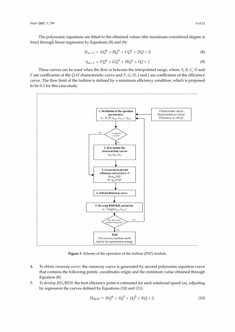
The polynomic equations are fitted to the obtained values (the maximum considered degree isfour) through linear regression by Equations (8) and (9):
Hα=1 = AQ4 + BQ3 + CQ2 + DQ + E (8)
ηα=1 = FQ4 + GQ3 + HQ2 + IQ + J (9)
These curves can be used when the flow is between the interpolated range, where A, B, C, D andE are coefficients of the Q-H characteristic curve and F, G, H, I and J are coefficients of the efficiencycurve. The flow limit of the turbine is defined by a minimum efficiency condition, which is proposedto be 0.3 for this case study.
Water 2017, 9, 799 6 of 21
= (5)
= (6)
η = ( ) (7)
The polynomic equations are fitted to the obtained values (the maximum considered degree is four) through linear regression by Equations (8) and (9):
= + + + + (8)
= + + + + (9)
These curves can be used when the flow is between the interpolated range, where A, B, C, D and E are coefficients of the Q-H characteristic curve and F, G, H, I and J are coefficients of the efficiency curve. The flow limit of the turbine is defined by a minimum efficiency condition, which is proposed to be 0.3 for this case study.
Figure 3. Scheme of the operation of the turbine (PAT) module.
3. To obtain runaway curve: the runaway curve is generated by second polynomic equation curve that contains the following points: coordinates origin and the minimum value obtained through Equation (8).
Characteristic curvesHead number;= fn()Efficiency; =fn()
1. Definition of the operation parameters:
ns , N, D , min, max y min.
3. Generate head and efficiency curves for=1
Q=intND3
H= intN2D2
4. O btain Runaway curve
5. Develop BEH/BEL points for = range(min, max)
2. Interpolate thecharacteristic curves
int-int-int
Is ns knownexactly?
No
Yes
Are there more turbine to generate?
Yes
No
ENDThe recovery machine can be
used in the optimization strategy
Figure 3. Scheme of the operation of the turbine (PAT) module.
4. To obtain runaway curve: the runaway curve is generated by second polynomic equation curvethat contains the following points: coordinates origin and the minimum value obtained throughEquation (8).
5. To develop BEL/BEH: the best efficiency point is estimated for each rotational speed (α), adjustingby regression the curves defined by Equations (10) and (11):
HBEH = HQ4 + IQ3 + JQ2 + KQ + L (10)

Water 2017, 9, 799 7 of 21
ηBEL = MQ4 + NQ3 + OQ2 + PQ + R (11)
where H, I, J, K and L characterise the best efficiency head and M, N, O, P and R are coefficientsthat define the best efficiency line.
2.3. Optimization Strategy
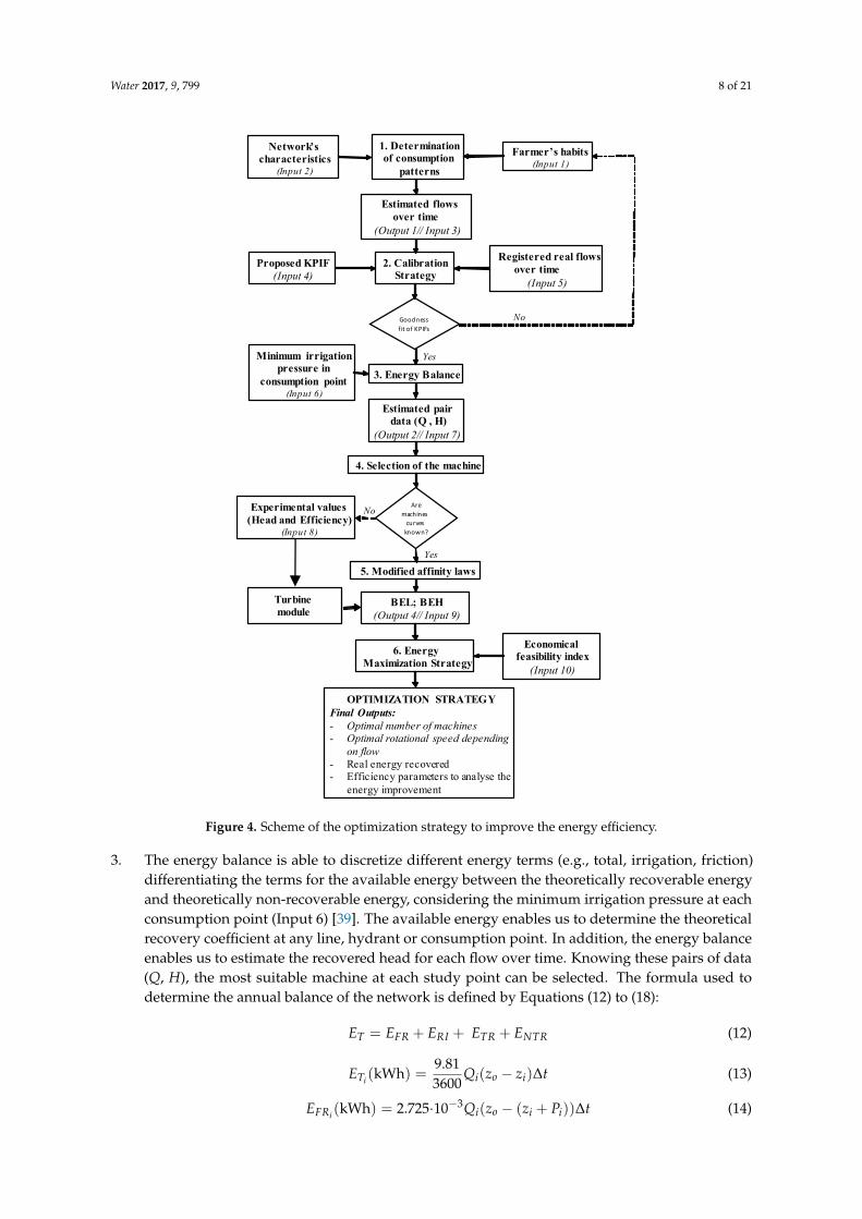
When the previously-cited material and methods are implemented, the development of theoptimization strategy to improve the energy efficiency in pressurized irrigation networks is possible.The development of this strategy makes sense since there are not any similar strategies for pressurizedwater distribution networks published in the expert literature. The developed optimization strategyfor the energy efficiency improvement is defined by different steps. This methodology needs differentinputs. The procedure is showed in the following flowchart (Figure 4).
1. The knowledge of the flow over time is the starting point in the optimization strategy. The flowcan be known when the water manager has flowmeters in the pipes. However, the knowledgeof the flow in all lines over time is almost impossible, and therefore, the flow has to beestimated in each line. In this sort of irrigation water distribution network, the flow depends onconsumption flow patterns which must be determined as a function of the agronomist parameters.To estimate the consumption flow patterns, the used methodology considers the farmers’ habitsand the characteristics of the network [39]. This methodology is able to estimate the flow overtime in any line of the systems, depending on the network characteristics (Input 1) and the farmers’habits (Input 2). The farmers’ habits are irrigation needs, irrigation duration, maximum daysbetween irrigation and the irrigation volume. The knowledge of the farmers’ habits allowsthe determination of the opening or closing in consumption nodes over time. The state ofthe irrigation point determines the flow (Output 1) of the strategy. This output is an input forthe next step: Input 3.
2. The second stage stands on the calibration strategy. It uses key performance indicators (KPIFs)that are adapted from the traditional hydrological models (Input 4) [40]. The characterization ofthe goodness-of-fit is divided into very good, good, satisfactory, and unsatisfactory, dependingon the KPIF values (Table 1). The comparison is developed with the registered flow data (Input 5)to determine the success of the fit. If the calibration is satisfactory, the energy balance (Step 3) canbe done.
Table 1. Classification of the goodness-of-fit (adapted from [40]).
Goodness-of-Fit E RRSE PBIAS (%)
Very Good E > 0.6 0.00 ≤ RRSE ≤ 0.50 PBIAS < ±10Good 0.40 < E ≤ 0.60 0.50 < RRSE ≤ 0.60 ±10 ≤ PBIAS < ±15
Satisfactory 0.20 < E ≤ 0.40 0.60 < RRSE ≤ 0.70 ±15 ≤ PBIAS < ±25Unsatisfactory E < 0.20 RRSE > 0.70 PBIAS > ±25
Water 2017, 9, 799 8 of 21Water 2017, 9, 799 8 of 21
Figure 4. Scheme of the optimization strategy to improve the energy efficiency.
3. The energy balance is able to discretize different energy terms (e.g., total, irrigation, friction) differentiating the terms for the available energy between the theoretically recoverable energy and theoretically non-recoverable energy, considering the minimum irrigation pressure at each consumption point (Input 6) [39]. The available energy enables us to determine the theoretical recovery coefficient at any line, hydrant or consumption point. In addition, the energy balance enables us to estimate the recovered head for each flow over time. Knowing these pairs of data (Q, H), the most suitable machine at each study point can be selected. The formula used to determine the annual balance of the network is defined by Equations (12) to (18): = + + + (12)
(kWh) = 9.813600 ( − ) (13)
1. Determination of consumption
patterns
Farmer’s habits(Input 1)
Estimated flows over time
(Output 1// Input 3)
Network’s characteristics
(Input 2)
Registered real flowsover time
(Input 5)
Proposed KPIF(Input 4)
Minimum irrigation pressure in
consumption point(Input 6)
Experimental values(Head and Efficiency)
(Input 8)
5. Modified affinity laws
BEL; BEH(Output 4// Input 9)
OPTIMIZATION STRATEGYFinal Outputs:- Optimal number of machines- Optimal rotational speed depending
on flow- Real energy recovered- Efficiency parameters to analyse the
energy improvement
Economical feasibility index
(Input 10)
3. Energy Balance
2. Calibration Strategy
No
Yes
Estimated pair data (Q , H)
(Output 2// Input 7)
4. Selection of the machine
Yes
No
6. Energy Maximization Strategy
Are machines
curves known?
Goodnessf it of KPIFs
Turbinemodule
Figure 4. Scheme of the optimization strategy to improve the energy efficiency.
3. The energy balance is able to discretize different energy terms (e.g., total, irrigation, friction)differentiating the terms for the available energy between the theoretically recoverable energyand theoretically non-recoverable energy, considering the minimum irrigation pressure at eachconsumption point (Input 6) [39]. The available energy enables us to determine the theoreticalrecovery coefficient at any line, hydrant or consumption point. In addition, the energy balanceenables us to estimate the recovered head for each flow over time. Knowing these pairs of data(Q, H), the most suitable machine at each study point can be selected. The formula used todetermine the annual balance of the network is defined by Equations (12) to (18):
ET = EFR + ERI + ETR + ENTR (12)
ETi (kWh) =9.813600
Qi(zo − zi)∆t (13)
EFRi (kWh) = 2.725·10−3Qi(zo − (zi + Pi))∆t (14)

Water 2017, 9, 799 9 of 21
ERIi (kWh) = 2.725·10−3QiPminIi ∆t (15)
ETRi (kWh) = 2.725·10−3Qi Hi∆t (16)
ETAi (kWh) = 2.725·10−3Qi(
Pi − Pmini
)∆t (17)
ENTRi = ETAi − ETRi (18)
where ET is the total provided energy in the network (kWh/year); EFR is the total friction energyin the network (kWh/year); ERI is the total required energy to irrigate correctly all consumptionpoints (kWh/year); ETR is the total theoretical recovered energy in the network (kWh/year);ENTR is the total unrecoverable energy in the network (kWh/year); ETi is the potential energy ineach irrigation point when the consumption in the network is null (kWh); EFRi is the dissipatedfriction energy until the irrigation point (kWh); ERIi is the required energy at the consumptionpoint to ensure the irrigation (kWh); ETAi is the available energy for recovery in a hydrant or line(kWh); ETRi is the maximum theoretical recoverable energy in an irrigation point, hydrant orline of the network, ensuring the minimum pressure of irrigation downstream (kWh); ENTRi isthe energy that cannot be recovered in a hydrant or line on the network (kWh); Qi is the flow bya line (m3/s); zi is the geometry level above reference plane of the irrigation point, consideringthe reference datum level (m); zo is the geometry level above the reference plane of the freewater surface of the reservoir (m); Pi is the service pressure in any point of the network whenconsumption exists (m w.c.); PminIi is the minimum pressure of service of an irrigation pointrequired to ensure the irrigation water evenly; and Hi is the value of the head of an irrigationpoint, hydrant or line (m w.c.). This head is obtained as Hi = Pi −max
(Pmini ; PminIi
); and ∆t is
the time interval (s).4. Knowing the flow (Qi) and recoverable head (Hi) over time from the energy balance (Output 2,
that is Input 7), enables the selection of the hydraulic machine type (e.g., radial, axial) accordingto the frequency histogram of the power generated among other conditions. To developa guaranteed estimation of the recovered energy, the head and efficiency curve as a functionof flow should be known for different rotational speeds (Input 8). If this information is notprovided by the manufacturer, experimental tests are recommended to obtain the efficiencyvariation depending on the flow and for different rotational speeds. However, if experimentaltests cannot be carried out, the experimental curves are determined using the characteristicnumbers (discharge and head number, Figure 1) to select a machine considering its specificspeed [41] using the turbine that was described in the previous section (Figure 2).
5. When the tests are carried or the characteristic curves are used, the modified classical affinity lawsbased on the variation of the specific parameters (discharge coefficient, q; head coefficient, h; andvelocity coefficient, n) can be used [33,42]. These parameters are defined by Equations (19) to (21):
h =HH0
(19)
q =QQ0
(20)
n =NN0
(21)
where H is the recovered head in m w.c.; Q is the flow through the turbine in m3/s whenthe rotational speed of the machine is N; and H0 and Q0 are head and flow, respectively, whenthe machine operates in its best efficiency point (BEP), for the rotational speed N0.
Based on modified classical similarity laws (when there are not experimental data), two newconcepts (the best efficiency line, BEL and best head line, BEH) are proposed (Output 4). The BELadapts the rotational speed as a function of the flow, adjusting the maximum efficiency at each time
Water 2017, 9, 799 10 of 21
point and maximising the energy recovered. The BEH relates the best efficiency point for each rotationalspeed with the recovered head as a function of the flow [35]. The knowledge of the BEL and/or BEH(Input 9) makes possible the use of these curves to develop the optimization of the energy recovery ona water system through the variation of the rotational speed as a function of the flow. The classicallaws are defined by Equations (22) to (24) [36]:
Q1
Q0=
(D1
D0
)3 N1
N0(22)
H1
H0=
(D1
D0
)2(N1
N0
)2(23)
P1
P0=
(D1
D0
)2(N1
N0
)3(24)
where Q1 is the flow in the new conditions of the rotational speed in m3/s; D1 is the diameter of theimpeller in the new N status in m; D0 is the nominal diameter of the impeller in m; N1 is the newrotational speed in rpm; H1 is the head in the new N status in m w.c.; P1 is the shaft power for each Nin kW; and P0 is the shaft power in the nominal condition in kW.
6. This new strategy to maximize the energy recovered was developed by using PATs or any typeof turbine. The theoretically recovered energy and the economic feasibility indexes (Input 10),particularly the simple payback period are considered (PSR) [39]. This strategy makes use ofa simulated annealing algorithm to carry out the optimization, selecting the best lines to installturbines as a function of the number of installed turbines in the water system. The optimizationcan be developed with two different functions: the first function only considers the recoveredenergy, while the second one analyses the ratio between recovered energy and PSR [35]. The finaloutput results of the optimization strategy are the optimal number of machines to install inthe network according to the objective function; the optimal rotational speed as a function ofthe flow; the real recovered energy; as well as the efficiency parameters to analyse the energyimprovement in the network.
3. Results and Discussion
The previously-described methodology was implemented in a real case study for an existingirrigation network. This network was located in Vallada (Valencia, Spain) and the water manager knewthe volume measurements for the final user points as well as main line flow measurements over time.
3.1. Case Study Description
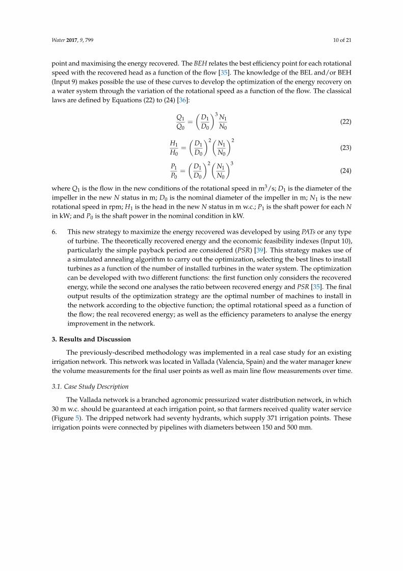
The Vallada network is a branched agronomic pressurized water distribution network, in which30 m w.c. should be guaranteed at each irrigation point, so that farmers received quality water service(Figure 5). The dripped network had seventy hydrants, which supply 371 irrigation points. Theseirrigation points were connected by pipelines with diameters between 150 and 500 mm.
Water 2017, 9, 799 11 of 21Water 2017, 9, 799 11 of 21
Figure 5. Characteristics and scheme of the water network.
3.2. Results of the Optimization
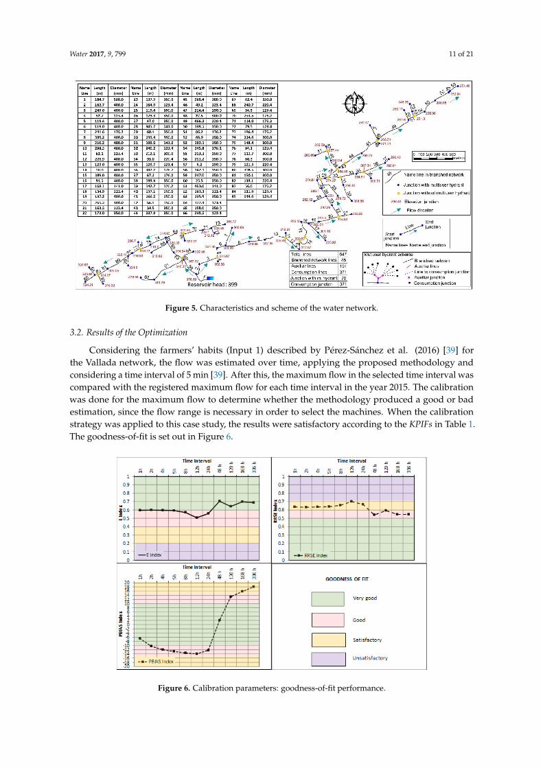
Considering the farmers’ habits (Input 1) described by Pérez-Sánchez et al. (2016) [39] for the Vallada network, the flow was estimated over time, applying the proposed methodology and considering a time interval of 5 min [39]. After this, the maximum flow in the selected time interval was compared with the registered maximum flow for each time interval in the year 2015. The calibration was done for the maximum flow to determine whether the methodology produced a good or bad estimation, since the flow range is necessary in order to select the machines. When the calibration strategy was applied to this case study, the results were satisfactory according to the KPIFs in Table 1. The goodness-of-fit is set out in Figure 6.
Figure 6. Calibration parameters: goodness-of-fit performance.
According to Table 1, the results performance was very good (0.6) when the time interval was between 1 and 5 h. When the time interval varied from 8 to 24 h, E values were between 0.50 and 0.56.
Figure 5. Characteristics and scheme of the water network.
3.2. Results of the Optimization
Considering the farmers’ habits (Input 1) described by Pérez-Sánchez et al. (2016) [39] forthe Vallada network, the flow was estimated over time, applying the proposed methodology andconsidering a time interval of 5 min [39]. After this, the maximum flow in the selected time interval wascompared with the registered maximum flow for each time interval in the year 2015. The calibrationwas done for the maximum flow to determine whether the methodology produced a good or badestimation, since the flow range is necessary in order to select the machines. When the calibrationstrategy was applied to this case study, the results were satisfactory according to the KPIFs in Table 1.The goodness-of-fit is set out in Figure 6.
Water 2017, 9, 799 11 of 21
Figure 5. Characteristics and scheme of the water network.
3.2. Results of the Optimization
Considering the farmers’ habits (Input 1) described by Pérez-Sánchez et al. (2016) [39] for the Vallada network, the flow was estimated over time, applying the proposed methodology and considering a time interval of 5 min [39]. After this, the maximum flow in the selected time interval was compared with the registered maximum flow for each time interval in the year 2015. The calibration was done for the maximum flow to determine whether the methodology produced a good or bad estimation, since the flow range is necessary in order to select the machines. When the calibration strategy was applied to this case study, the results were satisfactory according to the KPIFs in Table 1. The goodness-of-fit is set out in Figure 6.
Figure 6. Calibration parameters: goodness-of-fit performance.
According to Table 1, the results performance was very good (0.6) when the time interval was between 1 and 5 h. When the time interval varied from 8 to 24 h, E values were between 0.50 and 0.56.
Figure 6. Calibration parameters: goodness-of-fit performance.

Water 2017, 9, 799 12 of 21
According to Table 1, the results performance was very good (0.6) when the time interval wasbetween 1 and 5 h. When the time interval varied from 8 to 24 h, E values were between 0.50 and 0.56.The performance was always very good when the time interval was greater than 24 h. RRSE valueswere also analysed, and the goodness-of-fit was satisfactory when the time interval was between 1 and24 h. If the time interval was above 24 h, the performance was good. Finally, when the PBIAS indexwas analysed, the goodness-of-fit was very good for 1, 2, and 48 h. The calibration stage obtaineda good fit when the time interval was between 4 and 24 h. Satisfactory results were obtained whenthe time interval was 168 and 336 h.
Once the goodness-of-fit was verified using the KPIFs, the energy balance was applied. To do so,the proposed optimization strategy combined the energy balance (Step 3 in Figure 5); the selection ofthe machine (Step 4 in Figure 5), which is chosen through the database created using the proposedturbine generated (Figure 7); the modified affinity laws (Point 5 in Figure 5); and the maximizationstrategy (Step 6 in Figure 5) developed by simulated annealing algorithm.
Water 2017, 9, 799 12 of 21
The performance was always very good when the time interval was greater than 24 h. RRSE values were also analysed, and the goodness-of-fit was satisfactory when the time interval was between 1 and 24 h. If the time interval was above 24 h, the performance was good. Finally, when the PBIAS index was analysed, the goodness-of-fit was very good for 1, 2, and 48 h. The calibration stage obtained a good fit when the time interval was between 4 and 24 h. Satisfactory results were obtained when the time interval was 168 and 336 h.
Figure 7. Database of turbines created by the turbine module based on the experiments and affinity laws.
Once the goodness-of-fit was verified using the KPIFs, the energy balance was applied. To do so, the proposed optimization strategy combined the energy balance (Step 3 in Figure 5); the selection of the machine (Step 4 in Figure 5), which is chosen through the database created using the proposed turbine generated (Figure 7); the modified affinity laws (Point 5 in Figure 5); and the maximization strategy (Step 6 in Figure 5) developed by simulated annealing algorithm.
When the optimization strategy was performed, the recovered energy was maximized by selecting the machines operating under the best efficiency line. Table 2 shows from 1 to 10 lines of the selected machines as well as their location for each solution. In each selected pipe, three turbines with the same characteristic curves can be operated in parallel as a function of the flow at each time. Table 2 identifies the lines where the combination of turbines maximizes the objective function, indicating for each solution the specific speed of the machine, the impeller diameter and nominal rotational speed, as well as the recovered energy for each machine, which is shown using the best efficiency strategy ( ). In contrast, Table 3 shows the solution when the considered objective function is the ratio between recovered energy and PSR.
Figure 7. Database of turbines created by the turbine module based on the experiments and affinity laws.
When the optimization strategy was performed, the recovered energy was maximized by selectingthe machines operating under the best efficiency line. Table 2 shows from 1 to 10 lines of the selectedmachines as well as their location for each solution. In each selected pipe, three turbines with the samecharacteristic curves can be operated in parallel as a function of the flow at each time. Table 2 identifiesthe lines where the combination of turbines maximizes the objective function, indicating for eachsolution the specific speed of the machine, the impeller diameter and nominal rotational speed, as wellas the recovered energy for each machine, which is shown using the best efficiency strategy (ERBEL ).In contrast, Table 3 shows the solution when the considered objective function is the ratio betweenrecovered energy and PSR.

Water 2017, 9, 799 13 of 21
Table 2. Results of the maximization of the recovered energy (n is the number of pipes wherethe turbines are installed; ns in rpm (m, kW); D in mm; N in rpm; ERBEL in MWh/year).
n Lines in Which Turbines Are Allocated
1 382 22 383 22 38 594 22 38 47 595 5 22 38 47 596 5 22 38 47 58 597 5 22 38 47 58 59 708 5 22 38 39 47 58 59 709 2 10 22 39 43 47 58 59 7010 2 10 22 39 43 47 58 59 70 85
n TotalERBEL
1
nsDN
ERBEL
35114.3290033.78
33.78
2
nsDN
ERBEL
35133.8290030.97
35134.9290011.59
42.55
3
nsDN
ERBEL
35133.8290030.97
35134.9290011.59
35122.929003.56
46.11
4
nsDN
ERBEL
35133.8290030.97
35134.9290011.59
2990.529002.96
35122.929003.56
49.08
5
nsDN
ERBEL
44175.720409.81
35164.7290024.16
35134.9290011.52
2990.529002.96
35122.929003.56
52.00
6
nsDN
ERBEL
44175.720409.81
35164.7290024.16
35134.9290011.52
2990.529002.96
35100.629002.64
40121.229003.52
54.60
7
nsDN
ERBEL
44175.720409.81
35164.7290024.16
35134.9290011.52
2990.529002.96
35100.629002.64
35122.929003.56
2477
29000.83
55.47
8
nsDN
ERBEL
44175.720409.81
35164.7290024.16
35134.9290011.52
2460.429001.05
2990.529002.96
35100.629002.64
35122.929003.56
2477
29000.83
56.53
9
nsDN
ERBEL
83118.329008.27
35243.710206.22
35164.7290020.38
2477
29001.46
35134.9290010.73
2990.529002.96
35100.629002.64
35122.929003.56
2477
29000.83
57.04
10
nsDN
ERBEL
83118.329008.27
35243.710206.22
35164.7290020.38
2477
29001.46
35134.9290010.73
2990.529002.96
35100.629002.64
35122.929003.56
2477
29000.83
2671.529001.14
58.18

Water 2017, 9, 799 14 of 21
Table 3. Results of the maximization of the ratio between the recovered energy and PSR (n is the numberof pipes where the turbines are installed; ns in rpm (m, kW); D in mm; N in rpm; ERBEL in MWh/year).
n Lines in Which Turbines Are Allocated
1 38 382 22 38 223 5 22 38 54 5 22 38 60 55 5 22 38 56 60 56 5 10 22 38 58 60 57 5 10 22 27 38 58 60 58 1 5 12 13 22 38 58 60 19 1 5 10 22 38 48 58 54 60 110 1 5 6 8 10 22 26 38 58 60 1
n TotalERBEL
1
nsDN
ERBEL
2493.5290027.32
27.32
2
nsDN
ERBEL
3289.1290020.27
3576
24007.39
27.66
3
nsDN
ERBEL
7760
24005.21
3581.5290017.27
4177.124008.66
31.14
4
nsDN
ERBEL
7760
24005.21
3581.5290017.27
4177.124008.66
3568.720402.03
33.16
5
nsDN
ERBEL
7760
24005.21
3581.5290017.27
4177.124008.66
2443.829000.24
3568.720402.03
33.40
6
nsDN
ERBEL
6562.424005.12
40108.910203.60
4176.2290014.49
4177.124008.74
4053.624000.38
3568.720402.03
34.35
7
nsDN
ERBEL
6272.420405.57
40108.910203.60
4176.2290014.49
41107.45100.30
4063.329006.71
3847.429000.34
3568.720402.03
33.03
8
nsDN
ERBEL
65116.55101.01
7659.224004.94
40108.910202.95
3776.620400.20
4176.2290014.49
4177.124008.60
3449.229000.32
4358.524001.88
34.38
9
nsDN
ERBEL
65116.55101.01
7659.224004.94
40108.910203.16
4176.2290014.49
4072.224006.43
46106.85100.30
2447.724000.16
46106.85100.06
4358.524001.88
32.42
10
nsDN
ERBEL
65116.55101.01
6970.620405.37
41107.45100.07
4898.820400.15
39108.910203.04
4274.7290013.79
46106.85100.27
4063.329006.71
3947.729000.35
4358.524001.88
32.63

Water 2017, 9, 799 15 of 21
The comparison between both objective functions showed the main lines in which the recovery atmaximum were the same (e.g., lines 5, 22, and 38) in both simulations (i.e., the recovered energy andthe ratio between the recovered energy and PSR), but other lines were different. Therefore, the selectionof the objective function to optimize the water system will depend upon whether the feasibilityparameters are exactly known. In this case, in the optimization strategy considered for each selectedline (n) there were three PATs in parallel (so called PAT1, PAT2, and PAT3) and one bypass that wasopened by an isolation valve (here called IV4) to deviate the flow when the PAT cannot be operated.The pressure of the deviated flow is reduced by a pressure reduction valve (PRV1) (Figure 8a).
Water 2017, 9, 799 15 of 21
The comparison between both objective functions showed the main lines in which the recovery at maximum were the same (e.g., lines 5, 22, and 38) in both simulations (i.e., the recovered energy and the ratio between the recovered energy and PSR), but other lines were different. Therefore, the selection of the objective function to optimize the water system will depend upon whether the feasibility parameters are exactly known. In this case, in the optimization strategy considered for each selected line (n) there were three PATs in parallel (so called PAT1, PAT2, and PAT3) and one bypass that was opened by an isolation valve (here called IV4) to deviate the flow when the PAT cannot be operated. The pressure of the deviated flow is reduced by a pressure reduction valve (PRV1) (Figure 8a).
Figure 8. Operation scheme (a) and selected PAT (b).
The optimization strategy assigned the best machine for each assumption, chosen from the created database (8893 turbines), establishing the specific speed, the impeller diameter and the nominal rotational speed of the machine. The optimization strategy enabled knowledge for each solution of the next parameters, the operation time; work points and volumetric turbine flow for each machine. This was done once the recovered head as a function of flow was estimated applying the energy balance and using the EPANET Toolkit [35]. For instance, Figure 9a shows the pairs of data (i.e., flow and recoverable head) in line 47 when no PATs were installed upstream, as well as the recoverable points in line 47 when there were installed turbines in lines 5, 22 and 38, showing the dispersion of the operation zone.
This example was obtained when five groups of turbines (n = 5) were allocated in lines “5 + 22 + 38 + 47 + 59” and the maximization of the recovered energy was carried out (Table 2). Besides, Figure 9a shows the variation of the recoverable head as a function of flow when different group of turbines are installed in lines 5, 22, and 38. Figure 8b shows such an example, of the selected machine to install in line 47 inside of the group in parallel. The figure contains the obtained curves of the turbine: the runaway curve, the characteristic head curve for nominal rotational speed (α = 1), the efficiency curve for nominal speed, and the BEH and BEL curves. BEL was theoretically obtained by the PAT module and therefore the curve is horizontal. When this curve was developed by experimental tests, it was not horizontal and it was defined by a polynomic equation [35].
Figure 9b shows the flow values that were derived by the pass. The range for this selected machine varied between 0 and 2.19 L/s, and the total energy that could not be recovered because it was deviated was 124 kWh/year, guaranteeing the downstream pressure at all irrigation points over time. Besides, the figure shows the operation points when the PAT1 operated as well as its recovered head. For this machine, the volumetric turbine flow and the operation time were 36097 m3 and 1978 h, respectively. For PAT1, the average flow and the average recovered head were 5.06 L/s and 26.05 m w.c., respectively, obtaining an average power of 1.04 kW and a total recovered energy of 2047 kWh/year. Figure 9c,d show the recoverable energy values which were available to be operated throughout the PAT2 and the PAT3. The operation points are also shown in these figures for both PATs. Hence, the same values of volumetric turbine flow, operation time, turbine flow, recovered
Figure 8. Operation scheme (a) and selected PAT (b).
The optimization strategy assigned the best machine for each assumption, chosen from the createddatabase (8893 turbines), establishing the specific speed, the impeller diameter and the nominalrotational speed of the machine. The optimization strategy enabled knowledge for each solution ofthe next parameters, the operation time; work points and volumetric turbine flow for each machine.This was done once the recovered head as a function of flow was estimated applying the energybalance and using the EPANET Toolkit [35]. For instance, Figure 9a shows the pairs of data (i.e., flowand recoverable head) in line 47 when no PATs were installed upstream, as well as the recoverablepoints in line 47 when there were installed turbines in lines 5, 22 and 38, showing the dispersion ofthe operation zone.
This example was obtained when five groups of turbines (n = 5) were allocated in lines “5 + 22+ 38 + 47 + 59” and the maximization of the recovered energy was carried out (Table 2). Besides,Figure 9a shows the variation of the recoverable head as a function of flow when different group ofturbines are installed in lines 5, 22, and 38. Figure 8b shows such an example, of the selected machineto install in line 47 inside of the group in parallel. The figure contains the obtained curves of the turbine:the runaway curve, the characteristic head curve for nominal rotational speed (α = 1), the efficiencycurve for nominal speed, and the BEH and BEL curves. BEL was theoretically obtained by the PATmodule and therefore the curve is horizontal. When this curve was developed by experimental tests,it was not horizontal and it was defined by a polynomic equation [35].
Figure 9b shows the flow values that were derived by the pass. The range for this selected machinevaried between 0 and 2.19 L/s, and the total energy that could not be recovered because it was deviatedwas 124 kWh/year, guaranteeing the downstream pressure at all irrigation points over time. Besides,the figure shows the operation points when the PAT1 operated as well as its recovered head. For thismachine, the volumetric turbine flow and the operation time were 36,097 m3 and 1978 h, respectively.For PAT1, the average flow and the average recovered head were 5.06 L/s and 26.05 m w.c., respectively,obtaining an average power of 1.04 kW and a total recovered energy of 2047 kWh/year. Figure 9c,dshow the recoverable energy values which were available to be operated throughout the PAT2 andthe PAT3. The operation points are also shown in these figures for both PATs. Hence, the same values

Water 2017, 9, 799 16 of 21
of volumetric turbine flow, operation time, turbine flow, recovered head and power are also indicatedin Figure 9c,d. Finally, when the global values were analysed, the total volumetric turbine flow was53,420 m3, representing 98.71% of the volume throughout line 47. The minimum and the maximumturbine flow were 2.19 and 18.99 L/s, respectively. The total recovered energy was 2924 kWh/year,recovering 58.26% of the theoretical available energy of this line.
Water 2017, 9, 799 16 of 21
head and power are also indicated in Figure 9c,d. Finally, when the global values were analysed, the total volumetric turbine flow was 53,420 m3, representing 98.71% of the volume throughout line 47. The minimum and the maximum turbine flow were 2.19 and 18.99 L/s, respectively. The total recovered energy was 2924 kWh/year, recovering 58.26% of the theoretical available energy of this line.
Figure 9. Results of the operation zone and parameters of the volumetric turbine flow.
The increase of recovered energy was due to the use of the optimization strategy based on the best efficiency line of the selected machines. Figure 10a shows the different values of rotational speed (α) for each PAT as well as the total operation hours for each recovery machine. This figure shows that the nominal rotational speed represents only a few hours compared to the total turbine hours in each PAT. Therefore, the variation of the rotational speed for each machine was important to reach the maximum energy production in each time, considering the best efficiency line. Figure 10b shows an example in which the next items can be observed: the variation of speed coefficient (α), the generated power by recovery system over time in line 47. This figure also represents the pressure in node 47 that was downstream of the turbine, considering there are PATs in line 47, as well as showing the pressure when there are no turbines in this line.
Figure 10. Operation time, rotational speed, generated power and pressure in line 47.
Figure 9. Results of the operation zone and parameters of the volumetric turbine flow.
The increase of recovered energy was due to the use of the optimization strategy based on the bestefficiency line of the selected machines. Figure 10a shows the different values of rotational speed(α) for each PAT as well as the total operation hours for each recovery machine. This figure showsthat the nominal rotational speed represents only a few hours compared to the total turbine hoursin each PAT. Therefore, the variation of the rotational speed for each machine was important toreach the maximum energy production in each time, considering the best efficiency line. Figure 10bshows an example in which the next items can be observed: the variation of speed coefficient (α),the generated power by recovery system over time in line 47. This figure also represents the pressure innode 47 that was downstream of the turbine, considering there are PATs in line 47, as well as showingthe pressure when there are no turbines in this line.

Water 2017, 9, 799 17 of 21
Water 2017, 9, 799 16 of 21
head and power are also indicated in Figure 9c,d. Finally, when the global values were analysed, the total volumetric turbine flow was 53,420 m3, representing 98.71% of the volume throughout line 47. The minimum and the maximum turbine flow were 2.19 and 18.99 L/s, respectively. The total recovered energy was 2924 kWh/year, recovering 58.26% of the theoretical available energy of this line.
Figure 9. Results of the operation zone and parameters of the volumetric turbine flow.
The increase of recovered energy was due to the use of the optimization strategy based on the best efficiency line of the selected machines. Figure 10a shows the different values of rotational speed (α) for each PAT as well as the total operation hours for each recovery machine. This figure shows that the nominal rotational speed represents only a few hours compared to the total turbine hours in each PAT. Therefore, the variation of the rotational speed for each machine was important to reach the maximum energy production in each time, considering the best efficiency line. Figure 10b shows an example in which the next items can be observed: the variation of speed coefficient (α), the generated power by recovery system over time in line 47. This figure also represents the pressure in node 47 that was downstream of the turbine, considering there are PATs in line 47, as well as showing the pressure when there are no turbines in this line.
Figure 10. Operation time, rotational speed, generated power and pressure in line 47. Figure 10. Operation time, rotational speed, generated power and pressure in line 47.
3.3. Comparison of the Results of the Theoretical Energy Analysis, Fixed Rotational Speed, and BEL Strategy
Finally, the results of the proposed optimization strategy were compared with those obtainedwhen the theoretically energy was determined. Besides, the obtained energy from the proposedoptimization was also compared to the recovered energy, when the recovery machines only workedat their nominal rotational speed. Table 4 shows the obtained values when the maximization ofthe recovered energy was considered as an objective function. When the BEL strategy was applied(ERBEL), the generated energy varied between 33.78 and 58.18 MWh/year. These values representeda recovery coefficient between 37.41 and 41.66% of the theoretical recovered energy (ETR) that isconsidered when the efficiency of the machine is one (i.e., an ideal machine). The PSR varied between1.7 and 15.41 years from the one to 10 group of turbines (n), respectively. If the recovered energyusing the BEL strategy is compared to the recovered energy when the machine operated at a nominalrotational speed (ERα=1), the increase of the recovered energy varied between 140.88 and 183.79%.Therefore, the BEL strategy is one of the novelties introduced in this research, improving the energyrecovery under all assumptions when the energy recovery was compared with values for the machineunder nominal conditions.
Table 4. Comparison between recovered energy for the maximization of the recovered energy (ERBEL ,MWh/year; PSR, years; ER
PSRR, MWh; ER
ETR, %).
nBEL Strategy Theoretical Fixed Rotational Speed (α = 1)
ERBEL PSRRER
PSRRETR PSRTR
ETRPSRTR
ERETR
ER PSRRER
PSRR
ERBELERα=1
1 33.78 1.7 19.87 90.29 5.56 9.10 37.41 23.98 2.40 9.99 140.882 42.55 6.24 6.81 109.75 5.65 10.68 38.77 31.44 8.28 3.80 135.353 46.11 7.59 6.07 120.36 5.99 11.05 38.30 31.44 12.42 2.53 146.674 49.08 7.42 6.61 125.45 6.31 10.94 39.12 33.27 12.15 2.74 147.545 52.00 15.97 3.25 129.55 6.22 11.45 40.14 29.01 25.89 1.12 179.286 54.60 15.94 3.42 133.18 6.28 11.67 40.99 29.71 26.34 1.13 183.797 55.47 15.67 3.53 135.35 6.41 11.61 40.98 30.26 14.16 2.14 183.328 56.53 15.41 3.66 136.98 6.53 11.54 41.26 30.77 14.00 2.20 183.729 57.04 16.4 3.47 138.04 6.79 11.19 41.32 36.42 8.70 4.19 156.6410 58.18 16.16 3.60 139.64 6.85 11.21 41.66 36.98 8.63 4.29 157.33
Table 5 shows the results for the maximization of the ratio between recovered energy and simplepayback period. In this case, the ERBEL varied between 27.32 and 34.38 MWh/year. These values werelower than one for the maximization of the recovered energy objective function, and their reductionvaried between 56.08 and 80.87%. In this assumption, the difference of the recovered energy by usingthe BEL strategy was between 89.34 and 147.19% as a function of the number of groups of turbines (n)when the results were compared to ERα=1 .

Water 2017, 9, 799 18 of 21
Table 5. Comparison between recovered energy for the maximization of the ratio between the recoveredenergy and simple payback period (ER , MWh/year; PSR, years; ER
PSRR, MWh; ER
ETR, %).
nBEL Strategy Theoretical Fixed Rotational Speed (α = 1)
ERBEL PSRRER
PSRRETR PSRTR
ETRPSRTR
ERETR
ER PSRRER
PSRR
ERBELERα=1
1 27.32 0.71 38.46 49.66 5.46 9.10 55.01 11.78 1.65 7.14 147.202 27.66 0.59 46.82 60.36 5.65 10.68 45.83 13.66 1.20 11.38 113.833 31.14 0.6 51.71 62.61 5.58 11.23 49.73 16.74 1.12 14.94 107.794 33.16 0.61 54.01 68.24 5.87 11.62 48.59 17.83 1.14 15.64 114.545 33.40 0.61 54.03 69.68 5.96 11.69 47.93 17.95 1.15 15.60 115.696 34.35 0.65 52.34 70.95 5.98 11.87 48.41 20.02 1.13 17.78 101.127 33.03 0.64 51.03 70.95 5.98 11.87 46.55 19.48 1.10 17.70 95.248 34.38 0.72 47.24 70.93 5.95 11.94 48.47 21.64 1.19 18.18 89.359 32.42 0.66 49.10 71.05 5.95 11.95 45.62 19.75 1.08 18.28 87.0810 32.63 0.67 48.68 71.05 5.95 11.95 45.93 19.53 1.12 17.44 91.09
4. Conclusions
The paper presents a novel optimization strategy that enables the optimization of the recoveredenergy in any irrigation pressurized system by using the BEL strategy.
This optimization is based on optimizing the PAT operation, analysing the best efficiency line ofthe machine, and changing the rotational speed as a function of the flow at each time. Before definingthe rotational speed for each time, the strategy estimates the recovered head for each flow according tofarmers’ habits, which defines the flow pattern consumption for each irrigation point.
The estimation of the flow was calibrated according to KPIFs. This goodness-of-fit was good,or very good depending on the selected indicator. Besides, the strategy defined a database of turbinesaccording to characteristic parameters, which made possible the selection of the best turbine throughout forthe proposed PAT module when the water manager does not have available curves. Once the optimizationstrategy is used, the simulated algorithm processes allocate the machines in the best place bymaximizing the considered objective function and selecting suitable machines. This strategy presentedtwo different objective functions: the first function was the maximum recovered energy and the secondfunction was the ratio between maximum recovered energy and the simple payback period, obtainingfor each number of installed turbines the best lines to which to allocate them.
The analysed case study of a real water distribution system showed that the optimization strategycan be applied to any network when the farmers’ habits are known. This strategy was applied to reachthe installation of 10 turbine groups for both objective functions. The proposed methodology enabledknowledge of the operation points of the machine (flow, recovered head, efficiency and rotationalspeed) at each time and made it possible to reach the rotational speed necessary for each flow to obtainmaximum efficiency. This operation mode enabled us to increase the recovered energy to 183.79%when the BEL strategy was used, compared to the nominal rotational speed.
Similar results were obtained when the second objective function was used in the strategyand the values were compared with the results for the nominal rotational speed. In order to analysethe objective function, this second function (i.e., the ratio between recovered energy and simple paybackperiod), obtained very good feasibility indexes and will therefore be very interesting when the economiccost is known (e.g., installation, civil, maintenance). The PSR analysis showed that an increase inthe number of machines caused a growth of PSR value. When the PSR was analysed, iterations withmore than five PATs installed were not found to be feasible from an economic perspective. Whenthe objective function only considered the recovered energy, the analysis showed the maximizationwas viable for the installation of groups of machines. In contrast, if the maximization was developedconsidering the ratio between the recovered energy and simple payback period, lower feasibilityvalues were obtained for all assumptions.
Therefore, considering feasibility indexes within the maximization led to improved solutions.The installation of PATs in parallel was also considered in the cost analysis. This resulted in increased

Water 2017, 9, 799 19 of 21
advantages since their installation enabled an increased range of turbine flow, and therefore, increasedrecoverable energy.
In the analysed case study, the second objective function obtained recovered energy values thatincreased between 56 and 80% when this was compared to the first function, but obtained PSR valueslower than one, while the first function obtained a feasibility index between one and 16. Therefore,the strategy showed its effectiveness in allocating turbine to the best lines, in selecting the machines,and in looking for rotational speed on the BEL line in the maximization process, as well as in providingwater managers with alternatives to improve the energy efficiency in their water systems.
This strategy makes possible the development of more accurate energy recovery studies. In spite ofthis, future research should focus on the development of similar optimization strategies using meshedwater networks. Finally, relating to machine selection, future research should focus on the need tocorrelate the rotational speed and the specific speed using specific parameters (q, h, p, and e); this isof utmost importance for determining the real values of the BEL and BEH. This knowledge makespossible the successful selection of the best hydraulic machine by the proposed optimization strategydepicted in this research.
Acknowledgments: This research was supported by the program to support the academic career of the faculty ofthe Universitat Politècnica de València 2016/2017 in the project “Maximization of the global efficiency in PATsin laboratory facility” of the first author. Besides, the authors wish to thank to the project REDAWN (ReducingEnergy Dependency in Atlantic Area Water Networks) EAPA_198/2016 from INTERREG ATLANTIC AREAPROGRAMME 2014-2020 and CERIS (CEHIDRO-IST).
Author Contributions: All the authors participated in every step of this research. A brief description is attached:The author Helena M. Ramos contributed to correcting the manuscript and supervising the PAT analyses.Francisco Javier Sánchez-Romero was involved in the programming of the methodology for the development ofthe optimization strategy. Modesto Pérez-Sánchez proposed the optimization strategy as well as the used methodsand materials. P. Amparo López-Jiménez supervised the research and document and was involved in the finalenergy analysis of the results and conclusions proposal.
Conflicts of Interest: The authors declare no conflict of interest. The founding sponsors had no role in the designof the study; in the collection, analyses, or interpretation of data; in the writing of the manuscript, and inthe decision to publish the results.
Abbreviations
The following abbreviations are used in this manuscript:
BEH best efficiency headBEL best efficiency lineBEP best efficiency pointE Nash-Sutcliffe coefficientEFR friction energyER real recovered energyERI energy required for irrigationET total energyETA theoretically available energyETN theoretically energy necessaryETR theoretically recoverable energyENTR theoretically non-recoverable energyKPIF key performance indicatorsn number of groups of turbines or PATsns specific rotational speedPAT pump as working turbinePBIAS percent biasPSR simple payback periodRRSE root relative square error

Water 2017, 9, 799 20 of 21
References
1. Goonetilleke, A.; Vithanage, M. Water Resources Management: Innovation and Challenges in a ChangingWorld. Water 2017, 9, 281. [CrossRef]
2. Coelho, B.; Andrade-Campos, A. Efficiency achievement in water supply systems—A review. Renew. Sustain.Energy Rev. 2014, 30, 59–84. [CrossRef]
3. Nogueira, M.; Perrella, J. Energy and hydraulic efficiency in conventional water supply systems.Renew. Sustain. Energy Rev. 2014, 30, 701–714. [CrossRef]
4. McNabola, A.; Coughlan, P.; Corcoran, L.; Power, C.; Prysor Williams, A.; Harris, I.; Gallagher, J.; Styles, D.Energy recovery in the water industry using micro-hydropower: An opportunity to improve sustainability.Water Policy 2014, 16, 168. [CrossRef]
5. Lydon, T.; Coughlan, P.; McNabola, A. Pump-As-Turbine: Characterization as an Energy Recovery Devicefor the Water Distribution Network. J. Hydraul. Eng. 2017, 143, 04017020. [CrossRef]
6. Pasten, C.; Santamarina, J.C. Energy and quality of life. Energy Policy 2012, 49, 468–476. [CrossRef]7. Kanakoudis, V.; Papadopoulou, A. Allocating the cost of the carbon footprint produced along a supply chain,
among the stakeholders involved. J. Water Clim. Chang. 2014, 5, 556–568. [CrossRef]8. Kanakoudis, V.; Tsitsifli, S.; Papadopoulou, A. Integrating the Carbon and Water Footprints’ Costs in
the Water Framework Directive 2000/60/EC Full Water Cost Recovery Concept: Basic Principles towardsTheir Reliable Calculation and Socially Just Allocation. Water 2012, 4, 45–62. [CrossRef]
9. Kanakoudis, V. Three alternative ways to allocate the cost of the CF produced in a water supply anddistribution system. Desalin. Water Treat. 2015, 54, 2212–2222. [CrossRef]
10. George, B.; Malano, H.; Davidson, B.; Hellegers, P.; Bharati, L.; Massuel, S. An integrated hydro-economicmodelling framework to evaluate water allocation strategies I: Model development. Agric. Water Manag.2011, 98, 733–746. [CrossRef]
11. Huesemann, M.H. The limits of technological solutions to sustainable development. Clean Technol.Environ. Policy 2003, 5, 21–34. [CrossRef]
12. Sitzenfrei, R.; von Leon, J. Long-time simulation of water distribution systems for the design of smallhydropower systems. Renew. Energy 2014, 72, 182–187. [CrossRef]
13. Patelis, M.; Kanakoudis, V.; Gonelas, K. Pressure Management and Energy Recovery Capabilities UsingPATs. Procedia Eng. 2016, 162, 503–510. [CrossRef]
14. Patelis, M.; Kanakoudis, V.; Gonelas, K. Combining pressure management and energy recovery benefitsin a water distribution system installing PATs. J. Water Supply Res. Technol. AQUA 2017, 66, jws2017018.[CrossRef]
15. Patelis, M.; Vasilopoulos, I.; Kanakoudis, V.; Gonelas, K. Exploiting energy recovery potential in a waterdistribution network along with reliable pressure management. In Proceedings of the 13th InternationalConference on Protection and Restoration of the Environment, Skiathos Island, Greece, 3–8 July 2016;Volume 117–124.
16. Fecarotta, O.; Aricò, C.; Carravetta, A.; Martino, R.; Ramos, H.M. Hydropower Potential in Water DistributionNetworks: Pressure Control by PATs. Water Resour. Manag. 2015, 29, 699–714. [CrossRef]
17. Gilron, J. Water-energy nexus: Matching sources and uses. Clean Technol. Environ. Policy 2014, 16, 1471–1479.[CrossRef]
18. Emec, S.; Bilge, P.; Seliger, G. Design of production systems with hybrid energy and water generation forsustainable value creation. Clean Technol. Environ. Policy 2015, 17, 1807–1829. [CrossRef]
19. Okadera, T.; Chontanawat, J.; Gheewala, S.H. Water footprint for energy production and supply in Thailand.Energy 2014, 77, 49–56. [CrossRef]
20. Herath, I.; Deurer, M.; Horne, D.; Singh, R.; Clothier, B. The water footprint of hydroelectricity: A methodologicalcomparison from a case study in New Zealand. J. Clean. Prod. 2011, 19, 1582–1589. [CrossRef]
21. Baki, S.; Makropoulos, C. Tools for Energy Footprint Assessment in Urban Water Systems. Procedia Eng.2014, 89, 548–556. [CrossRef]
22. Kanakoudis, V.; Tsitsifli, S.; Samaras, P.; Zouboulis, A.; Demetriou, G. Developing appropriate performanceindicators for urban water distribution systems evaluation at Mediterranean countries. Water Util. J. 2011, 1,31–40.
Water 2017, 9, 799 21 of 21
23. Giugni, M.; Fontana, N.; Ranucci, A. Optimal location of PRVs and turbines in water distribution systems.J. Water Resour. Plan. Manag. 2013, 140, 6014004. [CrossRef]
24. Pérez-Sánchez, M.; Sánchez-Romero, F.; López-Jiménez, P.; Ramos, H. PATs selection towards sustainabilityin irrigation networks: Simulated annealing as a water management tool. Renew. Energy 2017, 116, 234–249.[CrossRef]
25. Corcoran, L.; McNabola, A.; Coughlan, P. Optimization of water distribution networks for combinedhydropower energy recovery and leakage reduction. J. Water Resour. Plan. Manag. 2015, 142, 4015045.[CrossRef]
26. Ramos, H.; Borga, A. Pumps as turbines: An unconventional solution to energy production. Urban Water1999, 1, 261–263. [CrossRef]
27. Ramos, H.M.; Kenov, K.N.; Vieira, F. Environmentally friendly hybrid solutions to improve the energy andhydraulic efficiency in water supply systems. Energy Sustain. Dev. 2011, 15, 436–442. [CrossRef]
28. Cabrera, J. Calibración de Modelos Hidrológicos. 2009. Available online: http://www.imefen.uni.edu.pe/Temas_interes/modhidro_2.pdf (accessed on 17 October 2017).
29. Moriasi, D.N.; Arnold, J.G.; Van Liew, M.W.; Binger, R.L.; Harmel, R.D.; Veith, T.L. Model evaluationguidelines for systematic quantification of accuracy in watershed simulations. ASABE 2007, 50, 885–900.[CrossRef]
30. White, F.M. Fluid Mechanics, 6th ed.; McGrau-Hill: Madrid, Spain, 2008.31. Kirkpatrick, S.; Gelatt, C.; Vecchi, M. Optimization by simmulated annealing. Science 1983, 220, 671–680.
[CrossRef] [PubMed]32. Samora, I.; Franca, M.; Schleiss, A.; Ramos, H. Simulated Annealing in Optimization of Energy Production
in a Water Supply Network. Water Resour. Manag. 2016, 30, 1533–1547. [CrossRef]33. Carravetta, A.; Del Giudice, G.; Fecarotta, O.; Ramos, H. PAT Design Strategy for Energy Recovery in Water
Distribution Networks by Electrical Regulation. Energies 2013, 6, 411–424. [CrossRef]34. Rossman, L.A. EPANET 2: User’s Manual; U.S. EPA: Ohio, OH, USA, 2000.35. Pérez-Sánchez, M. Methodology for Energy Efficiency Analysis in Pressurized Irrigation Networks, Practical
Application. 2017. Available online: https://riunet.upv.es/bitstream/handle/10251/84012/RESUMEN.pdf?sequence=3 (accessed on 17 October 2017).
36. Mataix, C. Turbomáquinas Hidráulicas; Universidad Pontificia Comillas: Madrid, Spain, 2009.37. Singh, P.; Nestmann, F. An optimization routine on a prediction and selection model for the turbine operation
of centrifugal pumps. Exp. Therm. Fluid Sci. 2010, 34, 152–164. [CrossRef]38. Derakhshan, S.; Nourbakhsh, A. Experimental study of characteristic curves of centrifugal pumps working
as turbines in different specific speeds. Exp. Therm. Fluid Sci. 2008, 32, 800–807. [CrossRef]39. Pérez-Sánchez, M.; Sánchez-Romero, F.; Ramos, H.; López-Jiménez, P. Modeling Irrigation Networks for
the Quantification of Potential Energy Recovering: A Case Study. Water 2016, 8, 234. [CrossRef]40. Pérez-Sánchez, M.; Sánchez-Romero, F.; Ramos, H.; López-Jiménez, P. Calibrating a flow model in
an irrigation network: Case study in Alicante, Spain. Span. J. Agric. Res. 2017, 15, e1202. [CrossRef]41. Pérez-Sánchez, M.; Sánchez-Romero, F.; Ramos, H.; López-Jiménez, P. Energy Recovery in Existing Water
Networks: Towards Greater Sustainability. Water 2017, 9, 97. [CrossRef]42. Fecarotta, O.; Carravetta, A.; Ramos, H.M.; Martino, R. An improved affinity model to enhance variable
operating strategy for pumps used as turbines. J. Hydraul. Res. 2016, 1686, 1–10. [CrossRef]
© 2017 by the authors. Licensee MDPI, Basel, Switzerland. This article is an open accessarticle distributed under the terms and conditions of the Creative Commons Attribution(CC BY) license (http://creativecommons.org/licenses/by/4.0/).