Embed Size (px)
Citation preview
Earnings Forecasts, Capital Budgeting and
The Abandonment Option
Jeffrey E. Jarrett, PhD.
Management Science and Finance
University of Rhode Island

Abstract
The abandonment option under various capital budgeting models are discussed in this
manuscript to bring forth the notion that present value of cash flows is often improperly estimated in
the financial models utilized in the decision analytic process. In this study, Intellectual Property Rights
and other intangible assets often are not considered in accounting estimation processes utilized in
financial accounting. A decision maker often utilizes misestimates of the present value of cash flow
resulting in less than optimum capital budgeting decisions. Decisions to abandon for salvage, and other
similar decisions improve when the present value of intangibles and property rights are included in the
decision process. This last statement is the goal of this study and to present well founded processes to
improve abandonment and similar decisions in capital budgeting decisions. The estimation problem in
financial accounting is included in the analysis to accomplish this goal.
Key Terms: Abandonment; Estimation Theory; Present Value of Cash Flow; Distribution of Earnings; Normal Fiducial Deviate; Opportunity Loss
Introduction Financial Researchers such as Deschow (1994, and Deschow and Strand, 2004) indicated that
employing accrual based accounting methods creates the capability of accounting based earnings
projections to control and continuously improve the measures of firm performance reflected in
analysts’’ earnings forecasts. The argument was that cash flow accuracy is expected to suffer from
matching, realization and other timing problems concerning the timing the recognition of costs and
revenues. Accuracy of financial earnings predictions was studied by (Brandon and Jarrett 1974;
Jarrett; 1983, Jarrett and Khumawala, 1987; and Jarrett, 1992 and Lambert et al. 2015). They
compared methods of forecasting accounting earnings seeking to learn how forecast models can be
compared and possibly improved to produce more accurate results as to cash flow. Questions posed
included sources of accuracy but accrual accounting alone was not considered the most important
source of inaccurate results. However, no one established a theoretical link between sources of
inaccuracy and the matching principle and the accuracy of financial analysts’ forecasts although
many studied the problem [Jarrett, 1989, 1990, Clement, 1999, Gu and Wu, 2003, Ramnath, Rock
and Shane, 2008 and Grosyberg et al. 2011]. Accounting reports containing these forecasts of cash
flow and rates of return are in addition, subject to fluctuations in the interpretation of timing
principles utilized by accountants. However, Gu and Wang (2005) brought up the possibility of
another source of inaccuracy in the forecast of rates of return, cash flow and earnings. Beneish et
al.(2013) created a model that uses financial ratios calculated with accounting data of a specific
company to check if it is likely that the reported earnings for a firm were manipulated. The goal being
to estimate earnings better in financial reports. Last, Lev and Gu (2016) in their study produced
evidence from large-sample empirical analysis, that financial documents' continuous deteriorate in
relevance to investors' decisions. Further, they detail why accounting reporting is losing relevance in
today's decisions related to capital budgeting and the abandonment option.
In this study, we examine how the presence of the abandonment option uses normal
capital budgeting methods to determine whether there is a relationship among the various
capital budgeting options, financial leverage and estimating earnings by analysts. We begin by
studying capital budgeting with the abandonment option, later most corporations use capital
budgeting procedures to coordinate and motivate activities throughout their organization. It is
well-understood that the budgeting process is dynamic and flexible, involving the information
flow throughout the organization that determines the investment and abandonment decisions
at the individual stages. We now examine at how an abandonment option influences the
optimal timing of information and vice versa. In particular, we compare timely information,
where the manager acquires perfect pre-contract project information. We examine how the
future revenues from intangible assets may affect the level of financial leverage of a firm when
not is all known about the economic value of intangible assets.
In the absence of the real option the following trade-off arises: if information is timely,
the investment decision can be based on perfect information. Alternatively, if information
about intangible assets is not considered in the abandonment option, the timing and decision
concerning the abandon option may very well be estimated incorrectly. The incorrect t
information is the product of the misreporting of factual events associated with intangible
assets and the error associated with incorrect analysts’ forecasts turn to the estimation
problem in financial accounting and in turn apply it to the relationship of analysts’ forecasts and
the bias in estimating earnings and cash flow present in evaluating capital decisions.
The Capital Budgeting Methodology
Berger et al. (1996) established the link among analysts’ forecasts, cash flow the
expected CAPM return, and the present value of cash flow which includes forecasts of earning
rather than the distributable cash flow. In addition, Wong (2009) examined the relation
between the abandonment option may affect a firm’s decision analysis and eventual the
analytics employed to determine the optimal decision and operating leverage. Furthermore,
McDonald (2003) analyzed abandonment options, divestment options, expansion options and
growth options previously examined in a survey by Triantis and Borison (2001). These and many
more studies revealed that they use real options to the general problems of the general
problems associated with capital budgeting.
Analysts’ earnings forecasts enable analysts to estimate the present value of cash flow
(PVCF). According to Berger et al. (1996), the advantage is that analysts’ forecasts of earning do
not incorporate the value of the abandonment option. If forecasts of distributable cash flows,
cash flows from non-ongoing concern events would be included in the forecasts. Thus, earnings
may not be the same as cash flows. Hence, we adjust because capital expenditures are not
equivalent to depreciation and the growth in working capital is not subtracted from earnings.
No longer is it required to adjust for capital structure changes in the environment that such
changes cannot be foreseen. Borrowing again from Berger et al. (1996), their equation
constructs the PVCF evolves from the analyst’s discounted forecasts. Included in the equation is
the includes sum of the present value of analysts' predicted going-concern cash flows discounted
by analyst forecast of year t after-interest earnings and expected CAPM (capital asset pricing
model return, consensus forecast of five year earnings growth, the terminal growth rate of
earnings, the number of years for which earnings are forecast and a year index. The capital
assets pricing model adjustment includes the reduction to the present value of analysts’
earnings. The second adjustment to PVCF is the working capital adjustment which is a reduction
to the present value of analysts' earnings forecasts to adjust for growth in working capital.
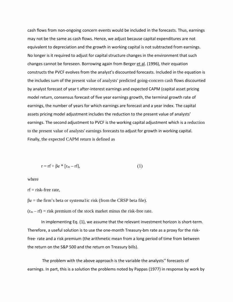
Finally, the expected CAPM return is defined as
r = rf + βe * [rm – rf], (1)
where
rf = risk-free rate,
βe = the firm’s beta or systema1ic risk (from the CRSP beta file).
(rm – rf) = risk premium of the stock market minus the risk-free rate.
In implementing Eq. (1), we assume that the relevant investment horizon is short-term.
Therefore, a useful solution is to use the one-month Treasury-bm rate as a proxy for the risk-
free· rate and a risk premium (the arithmetic mean from a long period of time from between
the return on the S&P 500 and the return on Treasury bills).
The problem with the above approach is the variable the analysts’’ forecasts of
earnings. In part, this is a solution the problems noted by Pappas (1977) in response by work by
Brief and Owen (1968, 1969, 1970 and 1977, Barnea and Sadan, 1974 and Jarrett (1983, 1992)
who used their work in developing models to adjust analyst’s’ earnings forecasts in evaluating
the abandonment option. Studies concerning analysts’ forecasts are well known and include a
huge number. In general, as stated by many others in the fields of financial accounting earnings
forecasts are dependent on the principles of financial accounting which produces the data for
modeling trends and seasonality (or modeling components). The accuracy of analyst forecasts
has a long history and includes by Clement, (1999) Gu and Wu (2003), Ramnath, Rock and
Shane, (2008), Groysberg et al., (2011) and Makridakis et al. (2017). The last manuscript
suggested that machine learning models may have better results that self-prepared models for
forecasting. These studies focused on a relationship between analysts’ forecasts and the
magnitude and value of intangible assets. Intangible assets were not considered in the
forecasting method discussed by the researchers in their many and detailed studies. The value
of intangible assets produces a great source of error if they are not considered in the
forecasting methods utilized by analysts in the production of cash flow, rates of return earning
per share forecasts. When adjustments for intangible assets are included in the analyst’s
forecasts, Gu and Wang (2005) stated that “The rise of intangible assets in size and contribution
to corporate growth over the last two decades poses an interesting dilemma for analysts. Most
intangible assets are not recognized in financial statement, and current accounting rules do not
require firms to report separate measures for intangibles.” (p.673, Gu and Wang, 2005).
Intangibles include trademarks, brand names, patents and similar properties that have value
but are generally not listed on financial reports of firms. Many of these items are technology
based and are very important in financial decisions such as in mergers and acquisitions. They
are an intricate in the growth of firms and therefore are shown to be related in the statistical
sense to the overall estimates made by accounting and analysts.
In another study concerning analysts’ forecasts, Matolesy and Wyatt (2006) found that
the association between EPS forecast, growth rates forecast error and measures of
technological conditions in the firm’s industry. They found as the forecast horizon increases, the
technological conditions and current EPS are statistically associated with analysts’ forecasts.
Long horizon creates the conditions for within one to conclude that interactions between
technological conditions and current EPS are associated with analysts’ EPS and growth
forecasts. This conclusion align itself with Jung, Shane and Yang (2012) who suggested that
analysts’ growth forecasts effect efforts to evaluate analysts’ forecasts may produce
optimistically biased long-term forecasts. Since intangible assets which are often technology
based are taken up more of the balance sheet of many firms, it is likely that analyst’s forecasts
may produce less accurate predictions of earnings, cash flow and rate of return. The
conclusions of Dechow (1992) become less important. Balance sheets usually have little or no
involvement with the value of intangibles although there are some practices by accounting are
still used. Thus in the remaining portions of this analysis, we propose a method by which one
can estimate earnings such that the value of intangible assets is valued and earnings estimate
are not biased by serious errors of omission such that the capital budgeting model expressed
earlier in equations by Berger et al. (1996, p. 264) are not unduly biased.
Intellectual Property and Traditional Accounting Methodology
As noted by [Brief and Owen 1969, 1970, 1977; Jarrett, 1971, 1974, and 1983; Roberts
and Roberts, 1970; and Barnea and Sadan, 1974;] the timing of recognition of revenue for IPR in
financial statements of ten are not featured in merger and acquisition activity. The financial
accounting standards board (FASB) provides for such activities, however, they are often ignored
due to their evasiveness or are not fully informational in there normally structured rules.
Recognizing future performance is a goal of matching and timing but are unrelated to
recognizing cash flow and similar items in the historical performance of a firm. Non-profit
entities often do not use accrual rules at all since the goal of these are related to achieving high
rates of return. Often IP rights for non-profits would differ from the same item for profit
maximizing entities since the goal of seeking high rates of return does not enter the strategic
planning process for non-profits {Definition of IPR: WTO, 2016}. The purpose here is to consider
IP as intangible assets as a product of intellect that law protects from unauthorized use by
those not responsible for the IP rights. Hence, IP rights are characterized as the protection of
distinguished signs such as trademarks for goods and services, patents, and other similar items
which are under protection from unauthorized use. This includes art, music, creations by

authors including the authorship of computer software and similar items such as discoveries,
inventions, phrases, symbols and design. Obviously, a writer and conductor of Music such as
Leonard Bernstein and Daniel Barenboim would have created IP that differ greatly from
Physicists such as Lisa Meitner, Nils Bohr or Albert Einstein.
Presently, accounting suggests two methods to determine the value of IP rights to
produce better estimates of from accounting analysts’ forecasts. The convention of the ‘lower
of cost or market” is based on the rule of conservatism in valuing assets to anticipate future
losses instead of future gains. The policy tens to understate rather than overstate the value of
net assets and could therefore lead to an understatement of income, cash flow, earnings and
rates of return. The purpose of this study and its conclusive result is to neither understate nor
overstate cash flow so as to produce a rate of return on cash flow that is commensurate with
the goal producing accurate prediction of cash flow and its rate of return for financial and
decision making purposes. Stated differently, the purpose is not to violate accounting policy but
to insure the mergers and acquisitions (M&A) that cash flow is estimated properly.
Traditionally, when accounting writes policy about intangible assets as a residual. By residual,
they mean a buyer is ready to value a firm in excess of the value of the tangible assets. This
value is often referred as Goodwill (White, et. al., 1994) which is an imperfect method. This
notion of goodwill is estimated as a residual value. If the valuation of intangible property is
imperfect since it considers part of the solution of a bargaining process. In this case, the buyer
and seller may have different market power which greatly affects the residual of the bargaining
process and produces an imperfect or biased estimate of the value of the intangible assets. One
may examine the case of the sale of “Superman” by struggling comic book artists to a much
larger corporate power who could market the character to “Comic Books”, Television and the
Film Industry. The nearly destitute conditions of the original artists who created the intangible
product could never cope with the business and marketing (power) of those who purchased the
name “Superman.” Thus, goodwill becomes a vague valuation system that justifies the bringing
of data analysis and science into the valuation process.
Another solution suggested during the M&A process is to simply list the patents,
trademarks, brands and similar items of IP in the financial reporting of the firm. Following this
initiative and suggestion of the accounting principles board provide little aid concerning the
economic value of IP rights and products for a firm during the M&A events. In the final step of
the problem the evaluation may conclude influence relating to the biases of the reading of the
financial reports. Such biases of IP occurred often with works of Meitner, Einstein and Bohr.
Whereas, at least Einstein and Bohr received Nobel Prizes which did have wealth, but Meitner
perhaps due to her gender and religious preference never received the award the others were
given. The three conductors and composers of music there was no economic award from the
Nobel Prize Committees. Accountants forecast the overall rate of return for a firm but do not
ignore the convention of “conservatism.” Accounting practice values the IP rights for a firm
each year for each and every IP right under consideration. The principle of Goodwill is not to be
used during M&A activity to account for the value of IP rights. IP may induce greater asset
values but also effects the rate of return on cash flow because the denominator of the rate of
return will change. [To understand the gravity of ignoring or improperly valuing IP rights see
Jarrett, 2016, 2017A and 2017B]. This result debated previously [Brief and Owen, 1969; Pappas’
1977 and Brief, 1977] indicated that including earnings risk may not fully reflect all risk in
estimating earnings, but at least, reflects that part of risk from the variation in earnings.
Furthermore, Helliar (et al. 2001) summarized attitudes of managers toward risk in the
following way. The abandonment option may be extremely appointment when considering the
survival of a firm or non-profit entity. Survival is often the goal of the abandonment option
indicating that risks that are taken in special situations such as catastrophes when the survival
of whole areas of an industry may be under threat (Liu and Liu, 2011 and Shleifer and Vishny,
1992) may be different from those taken in more usual environments. An entity in decline may
avoid innovative options and concentrate on immediate short-term options rather than riskier
longer-term projects with more difficult goals to be accomplished. In addition, the choice may
rapidly increase the rate up the process decline and result in managers becoming more risk
averse and not employing greater use of intangible assets and intellectual property.
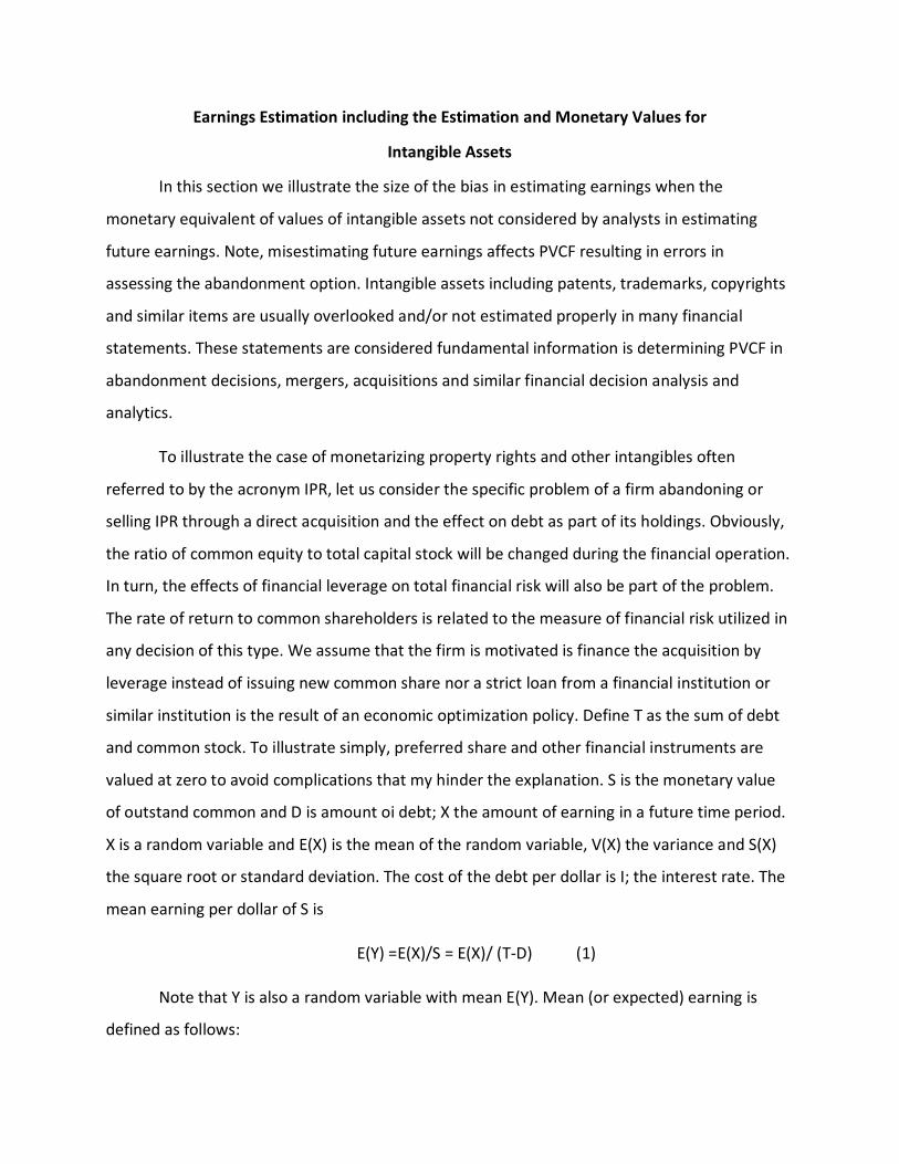
Earnings Estimation including the Estimation and Monetary Values for
Intangible Assets
In this section we illustrate the size of the bias in estimating earnings when the
monetary equivalent of values of intangible assets not considered by analysts in estimating
future earnings. Note, misestimating future earnings affects PVCF resulting in errors in
assessing the abandonment option. Intangible assets including patents, trademarks, copyrights
and similar items are usually overlooked and/or not estimated properly in many financial
statements. These statements are considered fundamental information is determining PVCF in
abandonment decisions, mergers, acquisitions and similar financial decision analysis and
analytics.
To illustrate the case of monetarizing property rights and other intangibles often
referred to by the acronym IPR, let us consider the specific problem of a firm abandoning or
selling IPR through a direct acquisition and the effect on debt as part of its holdings. Obviously,
the ratio of common equity to total capital stock will be changed during the financial operation.
In turn, the effects of financial leverage on total financial risk will also be part of the problem.
The rate of return to common shareholders is related to the measure of financial risk utilized in
any decision of this type. We assume that the firm is motivated is finance the acquisition by
leverage instead of issuing new common share nor a strict loan from a financial institution or
similar institution is the result of an economic optimization policy. Define T as the sum of debt
and common stock. To illustrate simply, preferred share and other financial instruments are
valued at zero to avoid complications that my hinder the explanation. S is the monetary value
of outstand common and D is amount oi debt; X the amount of earning in a future time period.
X is a random variable and E(X) is the mean of the random variable, V(X) the variance and S(X)
the square root or standard deviation. The cost of the debt per dollar is I; the interest rate. The
mean earning per dollar of S is
E(Y) =E(X)/S = E(X)/ (T-D) (1)
Note that Y is also a random variable with mean E(Y). Mean (or expected) earning is
defined as follows:

E (X’) = E(X) –iD for D>0; (2)
Hence, E (X’) = E(X), for D= 0 (2’)
The variance of total earnings is
V (X’) = V(X) for D≥0 (iD
and is a constant) (2’’)
The financial decision-optimum is to fund the purchase is an example of decision
analytics where the decisions are to substitute debt for common stock or not to substitute
debt. Using data analytical language, for this decision problem the states of nature are defined
by
E(X) >ID or E (X) ≤ ID (3)
We define the opportunity loss function as an integral approximation the firm’s view towards
choosing a non-optimal decision. No loss occurs when earnings are great than the cost of debt
since management will benefit from the strategy of leverage financing.
As an example consider cash flow to be greater than the cost of debt management and
in turn the loss function would change reflecting the goal of optimum decision analytics. The
basic structure of the acquisition strategy would not change except for the substitution of cash
flow for earnings. To calculate the opportunity loss function associated with this strategy, we
estimate some probability density function (PDF) that approximates the PDF for future
earnings. Before we consider all PDFs, let the firm focus on the normal distribution or T-
distribution having a very large number of degrees of freedom which approximates the
standard normal distribution. The opportunity loss becomes at breakeven (X b) becomes
X b = E (X’) - Z ((S (X’)) ; (4)
Z refers to the normal fiducial deviate; and S (X’) the standard deviation. By rearrangement, we
find E(X) = E (X’) – iD. The next step is to determine the size and distribution of the loss function
for the distribution of future earnings which is all in line with objectives of the timing of the
realization revenues discussed before Jarrett (1971, 1992). In Table 1 we preview one of three

methods to estimate the monetary value of IPR. The E(X) is $4200 and the S (X) increases by
given amounts ($100). Column 3 contains the cost of debt of $3200. The Z (the normal deviate)
calculation is accomplished column 4 with column 5 containing the cumulative normal
probability. In turn, the IPR monetary value is simply the normal probability multiplied by E (X)
and is contained in column 6. The IPR$ is thus calculated for a variety of circumstances.
Table 1
Monetarization of IPR
Changes in Standard Deviation of Earnings
E(X) S(X) Cost of Debt Z – Score Cum. Prob. $IPR 4200 400 3200 2.50000 0.993790 4174 4200 500 3200 2.00000 0.977250 4104 4200 600 3200 1.66667 0.952210 3999 4200 700 3200 1.42857 0.923436 3878 4200 800 3200 1.25000 0.894350 3756 4200 900 3200 1.11111 0.866740 3640 4200 1000 3200 1.00000 0.841345 3534
A second example of estimating the monetary value of IPR (Table 2, E(X), column 1 is
constant from row to row, column 2, S(X), remains the same ($600) from row to row and
column 3 the cost of debt changes from row to row due to the change in the interest rate and
other costs associated with debt. Column 4, the standard normal deviate, Z, decreases in value
from row to row and column 5, the cumulative probability from the normal curve decreases
from row to row. The dollar value of the IPR will continually decrease from the top row to the
bottom row in Table 2.
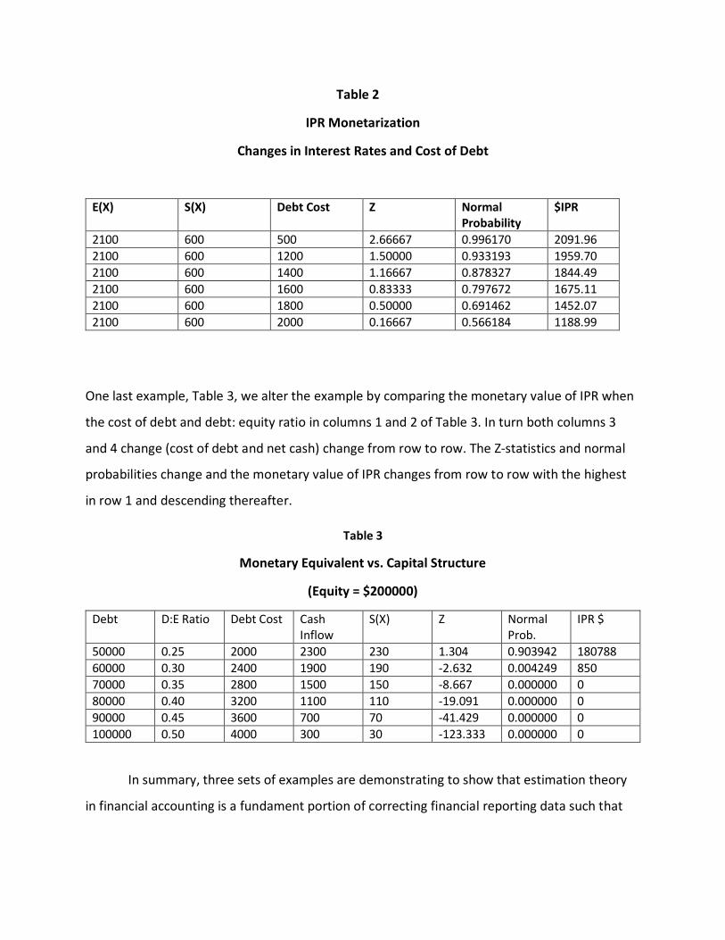
Table 2
IPR Monetarization
Changes in Interest Rates and Cost of Debt
E(X) S(X) Debt Cost Z Normal Probability
$IPR
2100 600 500 2.66667 0.996170 2091.96 2100 600 1200 1.50000 0.933193 1959.70 2100 600 1400 1.16667 0.878327 1844.49 2100 600 1600 0.83333 0.797672 1675.11 2100 600 1800 0.50000 0.691462 1452.07 2100 600 2000 0.16667 0.566184 1188.99
One last example, Table 3, we alter the example by comparing the monetary value of IPR when
the cost of debt and debt: equity ratio in columns 1 and 2 of Table 3. In turn both columns 3
and 4 change (cost of debt and net cash) change from row to row. The Z-statistics and normal
probabilities change and the monetary value of IPR changes from row to row with the highest
in row 1 and descending thereafter.
Table 3
Monetary Equivalent vs. Capital Structure
(Equity = $200000)
Debt D:E Ratio Debt Cost Cash Inflow
S(X) Z Normal Prob.
IPR $
50000 0.25 2000 2300 230 1.304 0.903942 180788 60000 0.30 2400 1900 190 -2.632 0.004249 850 70000 0.35 2800 1500 150 -8.667 0.000000 0 80000 0.40 3200 1100 110 -19.091 0.000000 0 90000 0.45 3600 700 70 -41.429 0.000000 0 100000 0.50 4000 300 30 -123.333 0.000000 0
In summary, three sets of examples are demonstrating to show that estimation theory
in financial accounting is a fundament portion of correcting financial reporting data such that
analysts now have a complete set of data work with when making earnings forecasts and other
decisions. Our finding does not dispute that of others.
Additional Evidence Concerning Estimation Theory and Methods
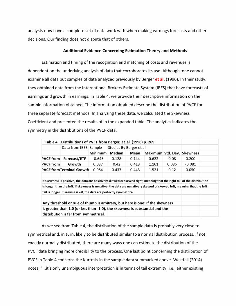
Estimation and timing of the recognition and matching of costs and revenues is
dependent on the underlying analysis of data that corroborates its use. Although, one cannot
examine all data but samples of data analyzed previously by Berger et al. (1996). In their study,
they obtained data from the International Brokers Estimate System (IBES) that have forecasts of
earnings and growth in earnings. In Table 4, we provide their descriptive information on the
sample information obtained. The information obtained describe the distribution of PVCF for
three separate forecast methods. In analyzing these data, we calculated the Skewness
Coefficient and presented the results of in the expanded table. The analytics indicates the
symmetry in the distributions of the PVCF data.
As we see from Table 4, the distribution of the sample data is probably very close to
symmetrical and, in turn, likely to be distributed similar to a normal distribution process. If not
exactly normally distributed, there are many ways one can estimate the distribution of the
PVCF data bringing more credibility to the process. One last point concerning the distribution of
PVCF in Table 4 concerns the Kurtosis in the sample data summarized above. Westfall (2014)
notes, "...it’s only unambiguous interpretation is in terms of tail extremity; i.e., either existing
Table 4 Distributions of PVCF from Berger, et al. (1996) p. 269Data from IBES Sample Studies By Berger et al.
Minimum Median Mean Maximum Std. Dev. SkewnessPVCF from Forecast/ETF -0.645 0.128 0.144 0.622 0.08 0.200PVCF from Growth 0.037 0.42 0.413 1.161 0.086 -0.081PVCF from Terminal Growth 0.084 0.437 0.443 1.521 0.12 0.050
If skewness is positive, the data are positively skewed or skewed right, meaning that the right tail of the distribution
is longer than the left. If skewness is negative, the data are negatively skewed or skewed left, meaning that the left
tail is longer. If skewness = 0, the data are perfectly symmetrical
Any threshold or rule of thumb is arbitrary, but here is one: If the skewnessis greater than 1.0 (or less than -1.0), the skewness is substantial and thedistribution is far from symmetrical.
outliers (for the sample kurtosis) or propensity to produce outliers (for the kurtosis of a
probability distribution)." The logic is simple: Kurtosis is the average (or expected value) of
the standardized data raised to the fourth power. Any standardized values that are less than 1
(i.e., data within one standard deviation of the mean, where the "peak" would be), contribute
virtually nothing to kurtosis, since raising a number that is less than 1 to the fourth power
makes it closer to zero. The only data values (observed or observable) that contribute to
kurtosis in any meaningful way are those outside the region of the peak; i.e., the outliers.
Therefore, kurtosis measures outliers only; it measures nothing about the "peak. Without the
original data, one cannot measure the exact Kurtoses for the data. However, one can observe
that the mean of data and minimum and maximum values do not differ by huge amounts.
Hence, the exact likelihood of long tails in the distribution of data about the mean do not exists.
The likelihood is therefore, such an observation indicates that if at all, the measures of Kurtoses
would be relative small and approach a normal distribution when examining the population
from which the sample was chosen. Hence, the normal approximation when the sample size is
large as in the cases observed indicates the validity of the normal approximation. Similarly, if
one has evidence that the data is distributed according to another probability distribution
function and that one could be used in evaluated the value of intellectual property rights.
Summary and Conclusion
Firms entering into decisions in times of financial distress are often confronted with failure and
survival. These decisions concerning the abandonment of assets. The problems associated with valuing
intangible assets and intellectual property rights are similar to those involved in decisions about mergers
and acquisition. The firm’s environment may different in each case, however the problems associated
with predicting cash flow and earnings by analysts still prevail. The study suggests ways of estimating the
earning and PVCF when considering the effects of intellectual property rights and other intangible assets
in the process. The proposal studied meets the requirements of the estimation theory in financial
account which is consistent with accounting conservatism and goals of financial accounting. Additional
methods exist for estimating the value of intangibles which include using the distribution of financial
earnings when the normal distribution does not apply. This will be the focus of new and additional
research.
References
Barnea A, and Sadan, S (1974) On the Decomposition of the Estimation Problem in
Financial Accounting. Journal of Accounting Research 12: 197-203.
Beneish, M.D., C.M.C. Lee and D. C. Nichols (2013), “Earning Manipulation and Expected
Returns,” Financial Analysts Journal, March/April2013:57-82.
Berger, P.G., E Ofek and I. Swary (1996) “Investor valuation of the abandonment
option,” Journal of Financial Economics, 42, 2, 257-287.
Brandon, C. and J.E. Jarrett (1974) “"Accuracy of Financial Forecasts," Financial Review,
9, 1 45; DOI:10.1111/j.1540-6288. 1974.tb01450.x; Abstract published in the CFA Digest,
summer, l975.
Brief, R and J. Owen (1968) "A Least Squares Allocation Model,” Journal of Accounting
Research, 23, 6,2, 193-199; DOI: 10.2307/2490234F
Brief R, and Owen J (1969)” A Note on Earnings Risk and the Coefficient of Variation,”
Journal of Finance,24: 4, 901-904.
Brief R, and Owen J (1970) “The Estimation Problem in Financial Accounting.” Journal of
Accounting Research 8: 167-177.
Brief R, (1977) “A Note on the Inclusion of Earnings Risk in Measures of Return: A
Reply,” Journal of Finance; 32 (4) 1367 DOI: 10.1111/j.1540-6261. 1977.tb03339.
Clement, M.B. (1999) “Analyst forecast accuracy: Do ability, resources, and portfolio
complexity matter?” Journal of Accounting and Economics, 27, 3, 285-303,
https://doi.org/10.1016/S0165-4101(99)00013-0
Deschow, P.M. (1994) “Accounting earnings and cash flows as measures of firm
performance; The Role of accounting accruals, Journal of Accounting & Economics, 18, 3-42

Deschow, P.M. and C. M. Schrand (2004) “Earnings Quality, “Research Foundation
Books, 3, 1-152. Gordon, M. and Halpern, A. (1974) “Cost of Capital for a Division of a Firm,”
Journal of Finance, 29, 4, 1153-1163, doi: 10.1111/j.1540-6261. 1974.tb03093.x
Gu, F. and Wang, W. (2005) “Intangible Assets, Information Complexity and Analysts
Earnings Forecasts,” Journal of Business Finance and Accounting, 32 (9) and (10), 1673-1702
Gu, Z. and Wu, J.S. (2003) “Earnings skewness and analyst forecast bias, Journal of
Accounting and Economics, 35, 1, 5-29 https://doi.org/10.1016/S0165-4101(02)00095-2
Groysberg, B., Healy, P., Nohria, N., and Serafeim, G. (2011) “What factors drive analyst
forecasts?” Financial Analysts Journal, 67(4), 18-29.
Hagendorff, J. & Hernando, I, Nieto, M J., and Wall, L. D., (2012). "What do premiums
paid for bank M&A’s reflect? The case of the European Union," Journal of Banking & Finance,
Elsevier, 36(3), 749-759.
Helliar, C., Lonie, A., Power, D. and D. Sinclair (2001) “Attitudes of UK Managers to Risk
and Uncertainty,” Balance Sheet, 9, 4, 7-10; DOI 10.1108/09657960110696717.
Jarrett J.E. (1971) “The Principles of Matching and Realization as Estimation Problems.
Journal of Accounting Research 9: 378-382.
Jarrett J.E. (1974) “Bias in Adjusting Asset values for Changes in the Price Level: An
Application of Estimation Theory.” Journal of Accounting Research 12: 63-66.
Jarrett J.E. (1983) “The Rate of Return from Interim Financial Reports, Journal of
Business Finance and Accounting 10: 289-294.
Jarrett, J. E. and S. Khumawala (1987) “A Study of Forecast Error and Covariant Time
Series to Improve Forecasting for Financial Decision Making,” Managerial Finance, 13(2):20-24

Jarrett, J. E. (1989) “Forecasting monthly earnings per share---Time Series Model,”
OMEGA: The International Journal of Management Science, 17, 1, 37-44.
Jarrett, J. E. (1990) “Forecasting Seasonal Time Series of Corporate Earnings: A Note,”
Decisions Sciences, 21, 4, 888-893.
Jarrett, J.E. (1992) "An Economical Method for Correcting Forecasting Error", American
Journal of Business, 7, 55-58, https://doi.org/10.1108/19355181199200017
Jarrett J.E (2016) “he Problems of Accounting Reporting False Information and
Estimation,” Intel Prop Rights. S1: 007.
Jarrett J.E (2017A) “Intellectual Property Valuation and Accounting.” Intel Prop Rights. 5:
181. Doi: 10.4172/2375-4516.1000181
Jarrett, J.E. (2017B) “Intellectual Property and the Role of Estimation in Financial
Accounting and Mergers and Acquisitions,” SF Journal of Intellectual Property Rights, 1:1, 1-8
Jung, B. Shane, F and Y. Yang (2012) “Do Financial Analysts’ Long-Term Growth Forecasts
Matter? Evidence from Stock Recommendations and Career Outcomes,” Journal of Accounting
& Economics (JAE), 51, 1-2
Lambert, D., Matolcsy, Z. and A. Wyatt (2015) “Analysts' earnings forecasts and
technological conditions in the firm's investment environment,” Journal of Contemporary
Accounting and Economics 11(2), 1-46 DOI: 10.1016/
Lev, B. and F. Gu (2016) The End of Accounting and the Path Forward for Investors and
Managers, Wiley, ISBN: 978-1-119-19109-4.
Liu, P. and C. H. Liu (2011) “The quality of real assets, liquidation value and debt
capacity,” [Electronic Article] The Center for Real Estate and Finance Working Paper Series,
2010-009, 1-43

Makridakis, S., E. Spiliotis and V. Assimakopoulos (2017) “The Accuracy of Machine
Learning (ML) Forecasting Methods versus Statistical Ones: Extending the Results of the M#-
Competition,” Working Paper, University of Nicosia, Institute for the Future, Greece.
Matolcsy, Z. and A. Wyatt (2006) “Capitalized intangibles and financial analysis,”
Accounting and Finance, 46, 457-479, DOI: 10.1111/j.1467-629x2006.00177x
Pappas, J.L. (1977) “A Note on the Inclusions of Earnings Risk in Measures of Return: A
Comment” Journal of Finance, 32 (4) 1363-1366.
Ramnath, S., Rock, S., & Shane, P. B. (2008). The financial analyst forecasting literature:
A taxonomy with suggestions for further research. International Journal of Forecasting, 24(1),
34-75.
Roberts, C. and E. Roberts (1970) “Exact Determination of Earnings Risk by the
Coefficient of Variation,” Journal of Finance, 25: 1161-1165.
Ramnath, S., Rock, S., & Shane, P. B. (2008). The financial analyst forecasting literature:
A taxonomy with suggestions for further research. International Journal of Forecasting, 24(1),
34-75.
Romanna, K. and R.L. Watts, (2012) “Evidence on the use of unverifiable estimates in
required goodwill impairment,” Review of Accounting Studies, 17, 4, 749-780
Schliefer, A. and R. W. Vishnay (1992) “Liquidation Values and Debt Capacity: Market
Equilibrium Approach,” Journal of Finance, XLVII, 4, 1343-1366.
White G.I, Sandhi A.C, and Fried D. (1994) The Analysis and Uses of Financial Statements
(3rdedn). John Wiley, New York
Wong, K. P. (2009) “The effects of abandonment options on operating leverage and
investment timing,” International Review of Economics & Finance, 18, 1, 162-171

WTO, 2016 "What are intellectual property rights?” World Trade Organization. World
Trade Organization
Jeffrey E. Jarrett [BBA, 1962, Michigan, MBA, 1963, PHD, 1967, NYU) is
nearing his fiftieth anniversary of receiving his doctoral degree from the newly named
Stern, Graduate School of Business Administration. Dr. Jarrett is the former Department
Chair of Management Science and is currently Professor of Management Science and
Finance at the College of Business/University of Rhode Island. He published extensively in The
Accounting Review, Decision Sciences, Journal of Business Finance and Accounting, Journal of
Accounting Research, Journal of Finance,
Management Science, OMEGA: The International Journal of Management Science,
Journal of Business Forecasting, Statistical Software Newsletter, Journal of Business and
Economic Statistics, Journal of the American Statistical Association, Atlantic Economic
Journal, Review of Business and Economic Research, Statistics and Computing, Journal
of Research in Economics and International Finance, Financial Engineering and Japanese
Markets, Economic and Financial Modelling, International Journal of Business and
Economics, and the International Journal of Forecasting Journal of Applied Statistics,
International Journal of Empirical Research, International Journal of Business and
Economics, Computational Statistics and Data Analysis, Communications in Statistics,
International Journal of Economics and Management Engineering and Applied Economics
among others. Further, he presented many research and summary papers at international
and national conferences. Currently, he is either a member of the editorial board or Editor in-
Chief, or Executive Editor of eight academic journals. Last, he published about 150
manuscripts in academic journals and authored (and coauthored about seven book

length manuscripts including several textbooks.