Inflation and Earnings Uncertainty

and Volatility Forecasts: A Structural Form Approach∗

Alexander David

Haskayne School of Business

University of Calgary

Pietro Veronesi

University of Chicago,

NBER and CEPR

March 2008

∗We thank George Constantinides, Ruslan Goyenko, Owen Lamont, Martin Lettau, Lubos Pastor, Simon Potter, Adriano

Rampini, Jeff Russell, Guofu Zhou, and seminar participants at the AFE meetings in New Orleans, NBER Summer Institute

Asset Pricing Workshop, the Federal Reserve Board, the Federal Reserve Bank of New York, the University of Chicago,

the University of Arizona, the Norwegian School of Business BI, the Copenhagen Business School, the University of

Brescia (Italy), and Washington University for insightful comments. Address (David): Address: 2500 University Drive

NW, Calgary, Alberta T2N 1N4, Canada. Phone: (403) 220-6987. Fax: (403) 210-3327. E. Mail: adavid@ucalgary.ca.

Address (Veronesi): Graduate School of Business, University of Chicago, 5807 South Woodlawn Avenue, Chicago, IL,

60637. Phone: (773) 702-6348. E-mail: pietro.veronesi@gsb.uchicago.edu. David thanks the SSHRC for a research grant.

Veronesi gratefully acknowledges financial support from the James S. Kemper Faculty Research Fund at the Graduate

School of Business, University of Chicago.

1

Inflation and Earnings Uncertainty and Volatility Forecasts: A Structural Form Approach

Abstract

We propose a new structural form methodology for understanding the fluctuations and pre-

dictability of volatilities and covariances of asset returns. In our model, a representative agent

learns about the joint movements in inflation and real earnings through business cycles. We ex-

tract investors’ beliefs about fundamentals from the prices and volatilities of stocks and bonds. The

duration of episodes of enhanced investors’ uncertainty are forecastable and lead to forecasts of

volatilities that are far more precise than those based on reduced-form models that include lags and

macroeconomic variables. The model’s success stems largely from endogenous and time varying

weights that investors assign to news about real fundamental growth and their pricing kernel.

JEL Classification Code: G10, G11, G12, G14

IntroductionOne of the most compelling findings in empirical finance research over the past three decades

is that volatilities of asset returns are highly persistent. The persistence property has been exploited

by the GARCH family of models that uses the information in current volatilities to forecast fu-

ture volatilities and has revolutionized the practice of portfolio management, risk management, and

derivatives. Despite the success of the volatility persistence paradigm, the empirical literature for

the economic mechanisms that cause this persistence is still at a relatively early stage. In addition,

the GARCH literature says little about the levels of asset prices themselves. In fact, an even earlier

school of thought starting with the work of Hayek (1945) and in its modern form under the Efficient

Markets Hypothesis of Fama (1970) argues that asset prices aggregate investors’ information. In its

weak form, the theory asserts that the information of investors contains the history of past prices.

Using this information, investors can formulate the relationship between current and past volatility,

and in turn, use current volatility to forecast future volatility. Since investors are likely risk averse,

their forecasts of volatility will affect current market clearing prices. Therefore, in principle, an

econometrician should be able to back out the volatility forecasts of investors from asset prices. In

this paper, we propose a structural form approach to volatility forecasting that explicitly extracts in-

vestors’ volatility forecasts and show that these forecasts substantially improve upon those obtained

from the GARCH-based model and its extensions that include various macroeconomic variables in

a reduced form way.

The canonical GARCH method of volatility forecasting is

f(σ2(t)) = β0 + β1f(σ2(t − 1)) + β2X(t) + ε(t), (1)

where σ2(t) is the variance of the asset in period t, f(·) is a possibly non-linear function often used

to make variance positive in this equation, X(t) is a vector of explanatory variables, and and ε(t) is

the shock to variance at time t. We call (1) the “reduced form” approach to volatility forecasting.

X(t) typically contains macroeconomic or price (returns) information. For example, in a reduced

form setup, Glosten, Jagannathan, and Runkle (1993) show that short term interest rates positively

forecast stock market volatility. Another popular X variable has been asset returns, especially

in periods when these returns are negative, resulting in the so called “leverage effect” [see, e.g.,

Black (1976)]. Schwert (1989) shows that recession dummies can forecast stock volatility better

than several other X variables, and Gennotte and Marsh (1993) find predictive power in lagged

volatilities of fundamentals. More recently the literature has moved towards studying the role of

macroeconomic factors in understanding the observed non-linearities in volatility dynamics. For

3

example, Boyd, Hu, and Jagannathan (2005) and Anderson, Bollerslev, Diebold, and Vega (2007)

show that the response of volatility to macroeconomic news depends on the state of the business

cycle, so that X(t) should contain more complicated functions of real fundamentals that can capture

the conditional state of the economy.

We raise three issues with such forecasting models. First, what is the role of including lags of

variances in the equation? Are these capturing the effects of persistence in the explanatory variables

X(t), or are these a parsimonious way of capturing the effect of all missing explanatory variables?

Second, what is the explicit mechanism by which these X factors impact volatility? For example,

despite there being fairly strong evidence for the effect of interest rates on volatility, the explanations

offered for the significance are anecdotal and not precisely quantified. Finally, since asset prices

should efficiently aggregate information1 why do they fail to be sufficient for forecasting volatility

on economy-wide stock indexes, leaving room for other variables, such as the current state of the

economy, to provide incremental forecasting power?

To address these issues we propose a new and different “structural form” approach to volatility

forecasting. In contrast to the GARCH literature, our approach starts from an economic specifica-

tion of fundamentals and investors’ pricing kernel – the main ingredients of an asset pricing model

– and explicitly solves for asset price levels and their volatilities in closed-form as functions of the

state variables of the model. The model is then fit not only to fundamental data, but also to asset

price levels and their volatilities with the use of overidentifying moments. Thus in our framework

the impact of the X variables on volatility is explicit and completely specified. It is important to note

that our approach is different from the traditional GARCH literature in not only specifying a func-

tional form for the volatilities of assets returns, but also in the way we fit our model parameters to

financial data. In the former literature, the volatility of historical asset returns is not observed by the

econometrician, who formulates alternative theoretical functional forms for volatility to maximize

the likelihood of observing the asset returns process. We instead follow an alternative approach in

the volatility literature of treating realized volatility as an observed process.2 This permits us to use1Indeed, empirical research has found that various interest rates measures that proxy for monetary policy are

perhaps the best predictors of the macroeconomy [see, e.g. Estrella and Mishkin (1998)].2In this sense we follow the approach of Schwert (1989) who approximated volatility at the monthly and quarterly

frequencies as the squared daily average returns in these periods, but did not have a structural specification of

volatility. More recently, there has been increasing interest in using higher frequency intra-day data to approxi-

mate volatility in any given period [see. e.g., Anderson, Bollerslev, Diebold, and Labys (2003)]. We continue to

use daily returns to construct our volatility measures since we are interested in studying the relationship between

volatility and the macroeconomy for a long sample during which intra-daily data are not available.

4

volatility as an overidentifying moment in our estimation procedure described above. Forecasts of

volatility can be optimally constructed using Monte Carlo simulations using the assumed dynamics

of the state variables of the economy and the estimated parameters of the structural form model.

In addition, our estimation procedure allows for the econometrician’s information set to be quite

different from that of investors, by allowing for signals and state variables being observed only by

the latter. Thus in our model, prices aggregate the signals received by investors as discussed in the

opening paragraph.

The economic mechanism in play in our analysis builds on the theoretical Bayesian learning

models of David (1997), Veronesi (1999), and Veronesi (2000), but significantly generalizes these

models by building in a joint macroeconomic relationship between nominal and real variables.

Suppose that inflation and the growth rates of real fundamentals in the economy jump erratically

between states and are not observable by investors. Instead, they must learn about these shifts from

observations of fundamental growth and prices and other signals. The states of inflation and real

growth are not independent, and information on the state of inflation helps investors formulate more

precise forecasts of real growth (and vice versa). Due to the noise in the fundamental processes,

investors take time to learn about these shifts, and during this learning period, they give more weight

to news and update their beliefs more rapidly. Asset prices, as the expected discounted value of

future fundamentals, will thus also become more volatile. If an econometrician is able to estimate

the frequency of shifts in average growth rates and the level of noise in fundamentals, then she can

predict how long the episode of increased uncertainty (volatility) will persist.3 Similarly, in periods3By “uncertainty” we mean a situation where investors are less than perfectly sure of some aspect of the con-

ditional data generating process (DGP) in any time period. In the model in this paper, investors only have

uncertainty of the drifts of the fundamental processes in the economy, which jump between a finite set of states.

Investors are Bayesian, and update their beliefs from observations of fundamentals and other signals. This defi-

nition of uncertainty is different from its use in the work of Bansal and Yaron (2004), who refer to uncertainty as

the conditional volatility of consumption growth, which affects risk premiums in asset pricing models. In com-

plete information settings similar to our paper, several authors have written regime-switching models of the term

structure and asset returns [see, e.g., Bansal and Zhou (2002), Ang and Bekaert (2002), Dai, Singleton, and Yang

(2003), Guidolin and Timmermann (2008). Our work is different in two respects: (i) we do not model regimes of

interest rates, but instead fundamental regimes (both real and inflationary), and (ii) the regimes are unobserved,

so that volatility of interest rates is endogenously determined in contrast to the above papers. Our definition, is

similar, but distinct from the ambiguity literature [see, e.g., Gilboa and Schmeidler (1989) or Epstein and Wang

(1994)] in which investors as in our model, do not have perfect knowledge of the DGP, but are also unable to put

conditional probabilities on the different possibilities. In such situations, investors are not Bayesian.

5

of low uncertainty, she can estimate the time for the next shift and episode of high volatility. Since

investors beliefs of the state of the fundamentals are common factors in the valuation of stocks

and bonds, covariances between their returns are also forecastable. In our empirical estimation, we

find that shifts of fundamental average growth rates occur at the business cycle frequency, causing

forecastability of volatilities and covariances up to a year.

The biggest success of our structural form model is in forecasting stock market volatility one

year ahead. Our model-based forecast doubles (from 18% to 38%) the explained future variation

of stock volatility relative to reduced form models that include lags and a host of macroeconomic

control variables, such as interest rates measures, fundamental volatilities, the state of the econ-

omy, stock returns and survey-based measures of investors’ uncertainty. The adjusted R2 improves

to 47% if the fourth quarter of 1987 in excluded, since the extreme volatility following the crash

of 1987 seems to be non-fundamental related. The set of controls used represent almost all the

variables used in the volatility forecasting literature. It is important to emphasize why our model’s

forecast is more successful than these other forecasts. First, our model utilizes the information

aggregation property of asset prices to capture the forward-looking information of investors in the

economy. Second, our structural model endogenously determines time-varying relative weights

given to news about inflation and earnings growth through different stages in the business cycle,

as it has been found by other authors. This relative weighting is important for our model to match

volatility fluctuations, because as we show, pure measures of inflation and earnings uncertainty have

low explanatory power for explaining stock volatility fluctuations. Finally, the model helps to tease

out investors’ expectations and uncertainty of fundamentals on a finer filtration than the simple

boom/bust states of a macroeconomic business cycle. In particular, our model calibration shows

that an important component of volatility, particularly in the 1960s and in the late 1990s, has been

the possibility of the US economy entering a new growth phase, which has also led to lofty stock

price valuations. The bursts of volatility in these episodes defies the common wisdom that volatility

is negatively correlated with stock prices, the so called “leverage effect.” Our model naturally gen-

erates this positive conditional correlation between stock prices and volatility, as investors’ upward

revision of their belief in a “new economy” regime raises both the expected earnings growth (which

pushes up prices) and the uncertainty about it (which pushes up volatility).

The model is successful in forecasting bond volatility as well, although its performance is less

spectacular than for stocks. In particular, model-implied bond volatility explains 73% and 66% of

the variation of one year and five year bonds, respectively. This is an increase in R2 of 10% and

6% over lagged volatility, respectively. However, unlike the case of stocks, a regression with both

6

model-implied volatility forecast and lagged volatility results in both variables being significant,

showing that our model does not capture all of the factors that affect bond return volatility. We

also find though that when we regress realized volatility on our model-based volatility forecast

and a set of macro variables, our variable keeps its strong statistical significance, while other macro

variables become often insignificant. This shows that our model-based forecast captures most of the

information in macroeconomic variables, although not all. Similar findings apply to the conditional

covariance between stocks and bonds. In short, our model-implied forecast of covariance alone

explains 60% and 50% of the variation of realized covariance for one year and five year bonds,

respectively. In addition, it is always highly significant in a regression with both lagged covariances

and other macro variables, although many of these other variables are significant as well. The main

difficulty of the model, we find, is to explain the strong negative covariance between stocks and

bonds in the beginning of the current decade. Although our fitted model does generate negative

covariance, the level is far smaller than that realized in the data. Indeed, outside of this period, our

model forecasts covariances over the remaining 40 years of our sample quite accurately. In line

with our results, Baele, Bekaert, and Inghelbrecht (2007) are also unable to explain the realized

negative covariance during this period using a broader set of macroeconomic variables than our

paper, but with a different empirical methodology that does not explicitly extract information from

asset prices. Following the suggestion in their paper we pursue the alternative channels of “flight-

to-safety” and “flight-to-liquidity” to explain the negative covariance in this period, but are unable

to explain its extreme movements with some popular measures of these variables. We provide a

further interpretation of this finding in the conclusion.

The paper develops as follows: in the next section we provide our economic model of fundamen-

tals, asset prices, and asset price volatilities. In section 2 we describe our empirical methodology to

estimate the model and discuss its implications for the time series of fundamentals and asset prices.

Section 3 contains our main findings: it performs the empirical tests on the forecastability of volatil-

ity and the covariation of asset returns. In section 4, we provide a detailed discussion the empirical

relationships between fundamental uncertainty, asset volatilities, and valuation ratios, and section

5 concludes. An appendix contains the details of our empirical methodology to estimate the pa-

rameters of our continuous time model with discrete data using the Simulated Method of Moments

(SMM).

7

1. Structure of the ModelIn this section we describe the structural model, which is fully described by Assumptions 1 - 8. The

model has several of the features in David (2006), which was used to price defaultable bonds.

Assumption 1. The price of the single homogeneous good in the economy, Qt, evolves according

to the process:dQt

Qt= βt dt + σQ dWt, (2)

where Wt = (W1t,W2t,W3t,W4t)′ is a four-dimensional vector of independent Weiner processes,

the 1 × 4 constant vector σQ = (σQ,1, σQ,2, 0, 0) is assumed to be known by investors, and the

process followed by βt is described below.

Assumption 2. Real earnings, Et, evolves according to the process:

dEt

Et= θt dt + σE dWt, (3)

where the 1 × 4 constant vector σE = (0, σE,2, 0, 0) is assumed known by investors and the process

for θt is described below.

Assumption 3. Investors observe unbiased signals, St, of the drift rate of earnings that follow the

process:dSt

St= θt dt + σS dWt, (4)

where the 1 × 4 constant vector σS = (σS,1, σS,2, σS,3, σS,4) is assumed known by investors. The

signals are not observed by the econometrician.

We use these fundamentals and the signal process to price all assets in our model. In order to

do so, we need to specify a stochastic discount factor to be used to discount real payoffs. We make

the following assumption:

Assumption 4. There exists a real pricing kernel Mt taking the form:

dMt

Mt= −ktdt − σM dWt, (5)

where σM = (σM,1, σM,2, σM,3, σM,4) is a 1 × 4 constant vector of the market prices of risk, and

kt = α0 + αθ θt + αβ βt, is the real short rate of interest. M is used to price real claims and

determine the expected real returns of all securities. We restrict the real rate of interest to be a linear

function of the two (hidden) state variables of the model.

8

The kernel is observed by investors but not by the econometrician. Using it, agents price a

generic real payout flow of Dt as:

MtPt = E

[∫ ∞

t

Ms Ds ds|Ft

], (6)

where Ft is investors’ filtration to be described in Assumption 5. As in several recent papers [e.g.,

Berk, Green, and Naik (1999) and Brennan and Xia (2002)], we have specified an exogenous pricing

kernel process to formulate equilibrium relationships among endogenous financial variables. The

linear dependence of the real rate on the drifts of fundamentals has a theoretical basis in general

equilibrium models: For example, in a Lucas (1978) economy where investors have power utility

U (C, t) = e−φt C1−γ

1−γ, we would have Ct = Et, Mt = U ′(Et), and hence ki = φ + γθi +

12γ (1 − γ) σEσ′

E and σM = γσE . In this case, the real rate is not affected by the inflation drift,

that is, αβ = 0. Our specification generalizes the real rate process to economies where expected

inflation affects the real cost of borrowing. This specification of the real rate can be supported in an

equilibrium if we allow a storage technology that can be bought or sold, is in perfectly elastic supply,

and offers a safe instantaneous return of kt. We provide further motivation for its dependence on

expected inflation next.

The literature on the effect of expected inflation on the real rate of return is extensive, and it

is beyond the scope of this paper to build in all the effects without significantly complicating our

analysis. David (2006) provides further description of these effects, some of which we describe

below. At the micro level there is a fairly large literature on various tax and accounting channels

through which expected inflation affects the real return on capital [Feldstein (1980a), Feldstein

(1980b), Auerbach (1979), and Cohen and Hassett (1999)]. Among the several monetary channels

that lead to the non-neutrality of money, of particular relevance are cash-in-advance models in

which expected inflation is a tax on money balances and raises the real cost of transactions, thus

affecting the real interest rate, capital accumulation, and business cycle variation [see Cooley and

Hansen (1989) for an empirical analysis of the size of this effect]. Given the multiplicity of channels

that affect the relationship between expected inflation and the real short rate, we treat the sign and

size of this relationship as an empirical question that can be estimated from the joint time-series

variation of fundamentals and asset prices. Our chosen functional form of the real rate can be seen

as a reduced form for the above noted effects.

For notational convenience, we stack the fundamental processes (2) and (3). Let Yt = (Qt, Et)′,

so that:dYt

Yt= %t dt + Σ2 dWt, (7)

9

where dYt

Ytis to be interpreted as “element-by-element” division, %t = (βt, θt)

′, and Σ2 = (σ′E, σ′

Q)′

Similarly, we find it useful to add the signal and kernel processes to the stacked vector and write

Xt = (Qt, Et,Mt, St)′, which has the drift vector νt = (βt, θt,−kt, θt)

′, and volatility matrix

Σ = (σ′Q, σ′

E ,−σ′M , σ′

S)′.

Assumption 5. νt follows an N−state, continuous-time finite state Markov chain with generator

matrix Λ, that is, over the infinitesimal time interval of length dt

λijdt = prob (νt+dt = νj|νt = νi) , for i 6= j, λii = −∑

j 6=i

λij.

The transition matrix over states in a finite interval of time, s, is exp(Λs) [see, e.g., Karlin and

Taylor (1982)].

Assumption 6. Investors do not observe the realizations of νt but know all the parameters of the

model.

Since investors do not observe νt, they need to infer it from the observations of past earnings,

inflation, the signal, and the pricing kernel. This learning process will generate a distribution on

the possible states ν1, ..., νN that in turn generates changes in “uncertainty” as they learn about the

current state. At time t, investors’ distribution over hidden states is summarized by the posterior

probabilities:

πit = prob(νt = νi|Ft),

where Ft is the filtration generated by observing the entire path (Xs)0≤s≤t. Let πt = (π1t, ..., πNt)

be the vector of beliefs.

Lemma 1. Given an initial condition π0 = π with∑N

i=1 πi = 1 and 0 ≤ πi ≤ 1 for all i, the

probabilities πit satisfy the N-dimensional system of stochastic differential equations:

dπit = µi(πt)dt + σi(πt)dWt, (8)

in which µi(πt) = [πtΛ]i, σi(πt) = πit [ νi − ν(πt)]′ Σ′−1

, (9)

ν(πt) =

N∑

i=1

πit νi = Et

(dXt

Xt

), and

dWt = Σ−1

(dXt

Xt− E

(dXt

Xt

)|Ft

)= Σ−1 (νt − ν(πt))dt + dWt. (10)

Moreover, for every t > 0,∑N

i=1 πt = 1.

10

Proof. See Wonham (1964) or David (1993).

The filtering theorem for jumps in the underlying drift was first derived (to the best of our knowl-

edge) in Wonham (1964). David (1993) provides a proof using the limit of Bayes’ rule in discrete

time. The first application of this theorem in financial economics, as well as several properties of the

filtering process, are derived in David (1997). In a parallel development in mathematical finance,

Elliott, Aggoun, and Moore (1995) provide results for this filtering process under an alternative

equivalent measure that simplifies the filtering process for some purposes.

We make the following summary comments about the updating process (8): (i) The elements

of the generator matrix, Λ, completely capture the transition probabilities between states. Absent

any new information, beliefs tend to mean-revert to the unconditional stationary probabilities that

are completely determined by Λ. For example, if there are only two states with λ12 = 2 and

λ21 = 1, then the belief that the economy is in state 1 mean reverts to 1/3. (ii) The diffusion term,

(νi − ν(πt)) (Σ′)−1, describes the magnitude of the change in beliefs due to uncertainty of each of

the components: inflation, earnings, and real rates. For example, the probability of being in state

i will reacts proportionately more to inflation shocks when the inflation rate in that state is further

away from investors’ conditional mean of inflation at that moment. In such periods investors revise

their beliefs more rapidly. Their beliefs are also more volatile in economies with lower noise in

fundamentals and higher precision of signals as captured in the (Σ′)−1 term. (iii) Agents update

their beliefs about underlying states by observing not only the path of fundamentals and signals, but

also their pricing kernel. This is analogous to the Lucas economy mentioned above in which the

agent would learn about the drift rate of the marginal utility of consumption.

It is useful to note that investor’s beliefs change with their inferred shocks, dW , in Equation (10)

as opposed to the true shocks, dW, that affect fundamentals. Similarly, they infer that the process

Xt follows: dXt/Xt = ν(πt)dt+ΣdWt. At each point in time, substituting the definition of dWt,

we have dXt/Xt = ν(πt)dt + Σ[Σ−1 (νt − ν(πt))dt + dWt

]= νtdt + ΣdW, which is the same

process as in Assumptions 1-3. In the filtering literature, dWt is an “innovations” process under the

investors’ filtration and under the separation principle it can be used for dynamic optimization. See

David (1997) for a discussion. As a special case we will write:

dYt

Yt= %(πt)dt + Σ2 dWt = %(πt)dt + Σ2 dWt, (11)

and the kernel under investors’ filtration as dMt/Mt = −k(πt)dt− σM dWt, where the real rate in

the economy, k(πt), is its expected value conditional on investors’ filtration.

11

1.1. Stock Prices and the Term-Structure of Interest Rates

For evaluating nominal claims and nominal risk premiums we will also use the nominal pricing

kernel, Nt = Mt/Qt, which follows:

dNt

Nt= −rtdt − σN dWt, (12)

where rt = kt +βt −σNσ′Q and σN = σM +σQ. The nominal rate differs from the real rate by the

sum of expected inflation and the inflation risk premium, which is the covariance between inflation

and the nominal pricing kernel. With unobserved states, the projected (observable) nominal interest

rate at time t is r(π) =∑N

i=1 ri πit, where ri = ki + βi − σNσ′Q is the nominal rate that would

realize in the i−th state, were the states observable. The following proposition provides expressions

for the Price-Earnings (henceforth P/E) ratio and the nominal bond price:

Proposition 1.

(a) The P/E ratio at time t is:

Pt

Et(πt) =

N∑

j=1

Cj πjt ≡ C · πt, (13)

where the vector C = (C1, .., CN ) satisfies C = A−1 · 1N ,

A = Diag(k1 − θ1 + σM σ′E , k2 − θ2 + σM σ′

E , · · · , kN − θN + σM σ′E) − Λ. (14)

(b) The price of a nominal zero-coupon bond at time t with maturity τ is:

Bt(πt, τ) =N∑

i=1

πit Bi(τ), (15)

Bi(τ) = E

(Mt+τ

Mt· Qt

Qt+τ|νt = νi

)=

[N∑

i=1

Ωi eωi τ

]· (Ω−1

1N ), (16)

where Ωi and ωi, i = 1, · · · , N, are the ith eigenvector and ith eigenvalue respectively of the matrix

Λ = Λ − Diag(r1, r2, · · · , rN ).

The proof follows from a simple extension of the proofs for stock and bond prices in Veronesi

(2000) and Veronesi and Yared (1999), respectively.

In (a), each constant Ci represents investors’ P/E valuation of stocks conditional on the state

being νi today. As in the classic Gordon model, the valuation depends on the expected growth of

earnings, the real rate, and the equity premium. Since investors do not observe the state νi, they

weight each Ci by its conditional probability πi thereby obtaining (13). Notice in particular that the

12

form of the constant vector C suggests that: (i) if αθ < 1, a higher growth rate of earnings implies

a higher P/E, (ii) if αβ > 0, a higher inflation state implies a lower P/E, which is the real rate

effect of inflation; and (iii) in addition, the P/E ratio in a given state of growth depends on the future

sustainability of the growth rate and is determined by the transition probabilities λij as shown in

the solution to the N -equations in (a).

Similarly, the bond price is a weighted average of the nominal bond prices that would prevail

in each state νi. Since investors do not actually observe the current state, they price the bond as

a weighted average. Both higher inflation and higher growth rate of earnings lead to lower long

term bond prices when αβ > −1 and αθ > 0. It’s useful to notice that all asset prices follow

continuous paths even though the drift rates for earnings and inflation jump between a discrete set

of states. This results from the continuous updating process.

Let P Nt = Pt · Qt, be the nominal value of stock, where Pt is the real value of stocks in

Proposition 1. Using the dynamics of the inflation and earnings processes under the observed

filtration, we now formulate the nominal return processes for stocks and bonds.

Proposition 2.

(a) The nominal stock return process under the investor’s filtration is given by

dP Nt

PNt

(πt) = (µN (πt) − δ(πt)) dt + σN (πt) dWt,

where δ(π) is the dividend yield, and the nominal stock price volatility is

σN (πt) = σE + σQ +

∑Ni=1 Ci πit (νi − ν(πt))

′(Σ′)−1

∑Ni=1 Ci πit

. (17)

(b) The nominal zero coupon bond return process is

dBt(πt, τ)

Bt(πt, τ)= µB(πt, τ) dt + σB(πt, τ) dWt,

where the nominal stock price volatility is

σB(πt, τ) =

∑Ni=1 Bi(τ)πit (νi − ν(πt))

′(Σ′)−1

∑Ni=1 Bi(τ)πit

. (18)

Proof. See Veronesi (2000) and Veronesi and Yared (1999).

Stock price volatility has an exogenous component due to noise in the fundamental process and

a learning-based endogenous component, which depends on the volatility of each state probability

πi. The volatility of each state probability depends on the fundamental uncertainties as discussed

in comment (ii) below Lemma 1. However, the volatility of stock prices depends additionally on

the valuation of stocks in each state as measured by the P/E vector, C . For a given news content,

13

states in which valuations are higher contribute more to the total volatility. Since the valuations

vary both with expected earnings growth and discount rates stock price volatility in our model will

endogenously load differently on news about these components in different stages of the business

cycle as found in Boyd, Hu, and Jagannathan (2005). If for example, in state 5 the earnings drift

is far from its value in other states, so that the volatility of the probability of this state is most

reactive to earnings news, then stock volatility will give a larger weight to this earnings news if P/E

ratios are high in this state, which will result if the earnings drift is larger than those in other states.

Alternatively, if the earnings drift is smaller than in the other states, then the weight of earnings

news in the stock volatility will be diminished. We will discuss this point further in Section 2 for

our calibrated model.

The form of the bond volatility equation is very similar to the stock volatility equation, except

that the P/E ratio in any state is replaced by the bond price in that state. In addition, there is no

exogenous fundamental component to bond volatility. The two volatility equations (17) and (18)

are the heart of this paper. From these, covariances between stocks and bonds, and bonds of different

maturities are derived straightforwardly. For example, the former is

Cov(

dP Nt (πt)

PNt (πt)

,dBt(πt, τ)

Bt(πt, τ)

)= (σE + σQ)σB(πt, τ)′ (19)

+

∑Ni=1

∑Nj=1 πit πjt Ci Bj(τ)(νi − ν(πt))

′ (ΣΣ′)−1 (νi − ν(πt))∑N

i=1

∑Nj=1 πit πjt Ci Bj(τ)

.

2. EstimationIn this section we provide a brief description of the estimation methodology and the parameter

estimates of our model.

2.1 Estimation methodology

We estimate the model by using information in both and first and second moments of financial vari-

ables to obtain the time-series of investors’ beliefs over fundamental states, as well as the underlying

parameters using a simulation based SMM method as described below.

Let Ψ denote the set of structural parameters in the fundamental processes of inflation, earnings,

earnings signals, and the pricing kernel in Equations (2), (3), (4), and (5), respectively. Let the

likelihood function for the fundamentals data observed at discrete points of time (quarterly) be L.

To extract information about investors’ beliefs from financial variables and their volatilities, we use

14

the pricing formulae for the P/E ratio and Treasury bond prices in Proposition 1 and their volatilities

in equations (17) and (18) to generate model-determined moments. Let e(t) denote the errors of

the pricing and volatility variables, and define ε(t) =(e(t)′, ∂L

∂Ψ(t)′)′

, where the second term is

the score of the likelihood function of fundamentals with respect to Ψ. We now form the SMM

objective:

c =

(1

T

T∑

t=1

εt

)′

· Ω−1 ·(

1

T

T∑

t=1

εt

). (20)

The details of the procedure are in the Appendix.

2.2 Estimation results for the regime switching model

In this subsection, we briefly describe the results of our estimation of our model. We start with

the description of the data series used. Our data sample runs from 1960-2006. Aggregate earnings

for the economy are approximated as the operating earnings of S&P 500 firms, and these data are

obtained from Standard and Poor’s. Similarly, the aggregate P/E ratio is estimated as the equity

value of these firms divided by their operating earnings. Dividends for these firms, also obtained

from Standard and Poor’s, are used with the prices to compute returns. We use the Consumer Price

Index (CPI), obtained from the Federal Reserve Bank of St. Louis, as our inflation series, which is

used both for discounting nominal earnings, as well as for forecasting future real earnings using our

joint regime switching model of fundamentals. The time-series of zero coupon yields and returns on

bonds of different maturities are obtained from the Fama-Bliss data set available at the University

of Chicago. Finally, the realized volatilities of stocks and bonds are estimated as squared average of

daily returns in any given quarter. Returns are non de-meaned, although the de-meaning of the series

does not significantly affect our results. Use such daily averages has a long tradition in finance [see,

e.g., Schwert (1989)]. More recently, authors such as Anderson, Bollerslev, Diebold, and Labys

(2003) have used higher frequency intra-daily data to estimate realized volatilities, however, such

data are not available for the long sample that we use.

We estimate a model with three regimes each for inflation characterized by the states β1 <

β2 < β3, and earnings growth, θ1 < θ2 < θ3, which lead us to nine composite states over-

all. In our estimation, we found that the unconstrained estimates of the transition matrix led to

several zero elements, leading to a more parsimonious five state model with the following states:

(β1, θ2), (β2, θ1), (β2, θ2), (β3, θ1), (β1, θ3). We found that the remaining four states had close

to zero probability of occurring in the sample. Overall, the five state and nine state model lead to

almost the same value for the SMM objective function. Gray (1996) and Bansal and Zhou (2002)

15

use a similar criterion for the choice among alternative regime specifications.

The top panel of Table 1 reports the means and volatilities of fundamentals, as well as the

pricing kernel parameters. The middle panel reports the transition probability matrix, as well as

the asset prices in the four states. We estimate that inflation averages 2.1%, 4.1%, and 8.4% in the

three states, which we shall refer to as low (LI), medium (MI), and high (HI) states of inflation.

Earnings growth averages -3.5% and 2.5% and 5.4% which we classify as regular low (LG) and

high (HG) growth rate states, and the “new economy” (NG) growth rate states, respectively. We

provide further motivation for the names give to these states by looking at the implied quarterly

and five-year transition probability matrices in the top two panels of Table 2. These matrices are

derived solely from the elements of the generator elements in Table 1. We provide some summary

descriptions next.

Notice first that the the regular high growth rate of earnings, θ2, is far more persistent in the low

inflation state: from the (LI-HG) state, there is a 99% chance of returning to this state, and a 1%

chance of transitioning to the (MI-HG) state in a quarter, therefore there is almost a zero chance

of growth slowing in a quarter in which there is also low inflation. From the (MI-HG) state on the

other hand there is an 2.2% chance of a transition to the (MI-LG) state in the following quarter.

This is the signaling role of inflation – it provides an early warning signal of an unsustainable

high growth rate of fundamentals. Second, we see from the bottom panel of Table 2, that by our

model estimates, regular high growth rates (states 1 and 3) would occur in about 70 percent of

the time and the regular low growth states would occur in about 27.5 percent of the time. In fact,

in a model with a similar structure, David (2006) show that these four states provide a good fit

for fundamentals and credit spreads. However, including short term (quarterly) stock volatility as

one of the overidentifying conditions, leads to a rejection of the four state model. We will see

shortly that this failure is largely due to the spectacular rise of stock volatility in the late 1990s and

its equally spectacular fall in the first half of the current decade. These massive swings seem to

be unrelated to the transitions of the economy between the four basic macro states as seen in the

time-series of implied investors’ state probabilities that are shown in Figure 1. Overall, as seen,

investors have held fairly strong views that the US economy has remained in the LI-HG states. For

most of the decade of the 1960s this probability hovered 85 percent percent, while in the 1990s it

was lower at around 70 percent. There were several switches within the medium inflation states

in the 1970s, with two bouts of high inflation and low growth in the mid-1970s and early 1980s.

The mid to late 1980s were characterized by high (nearly 40 percent) probabilities of the MI-HG

state, which steadily declined through the end of the 1990s, although the probabilities of this state

16

rose substantially to about 35 percent before the recession in 1990. This trend decline in expected

inflation has also been noted by other authors [see, e.g. Sargent, Williams, and Zha (2006)]. In

the current decade, the probability of the MI-HG state has slowly trended up and has averaged

about 5 percent in 2002-2005. Unlike all previous recessions, the biggest reassessment in investors’

expectations in the 2001 recession related to earnings growth rather inflation, as investors sharply

revised their beliefs that the economy was in the NG (fifth) state. We discuss the implications of

this revision further below.

The fifth state, (LI-NG), has a stationary (long-run) probability of only about 2.5%, but its in-

clusion in our model helps to a large extent to explain the high P/Es and high stock market volatility

in the late 1990s. During this period, earnings growth was far above its historical average, and led

investors to conjecture that due to productivity increases, there was a “new economy growth rate.”

As we see from investors filtered probabilities in Figure 1, investors were very uncertain that the

economy was in this state, which led to high stock market volatility. In this sense, the experience of

the late 1990s was extraordinary: while earnings grew rapidly in the 1960s as well, the probability

to the NG state only briefly touched 5 percent, while in 1999 it reached 25 percent. This channel

of expectations of high growth rates causing the high P/Es and high volatility in the 1990s was also

used by Pastor and Veronesi (2006). As in their model, we see in Proposition 1 that PEs are convex

in expected growth rates of earnings, which implies that in periods of higher uncertainty, ceteris

paribus, PEs are higher. However, their paper did not analyze the longer term relationship between

uncertainty, PEs, and volatility. Examining the time series of uncertainty though, we see that in all

other periods of high uncertainty in our sample, PEs were low, because in such periods investors

feared a recession of the economy and had low expectations of earnings growth. Finally, it is also

useful to note by our model estimates, the new economy growth only occurs in low inflation states,

so that a pickup in inflation lowers investors’ assessed probability that the new economy growth

will persist. As seen in Figure 1, the slight trend increase in the probability of the MI-HG state in

the current decade has been accompanied by a steady decline in the probability of the LI-NG state.

The low probability of occurrence of the high drift rate of earnings lends some similarity of our

model estimated parameters to the recent work on “long-run risks” starting with the work of Bansal

and Yaron (2004). This channel is used to generate a large equity premium in their paper. In our

model, investors are confronted with the possibility that a low probability switch of fundamentals

occurred in the late 1990s. As it can be seen from the middle panel of Table 2, even at the five-year

horizon there is only about a one percent chance of the economy entering the NG state from any

other state. This low probability explains why investors filtered probability of this state reached

17

a maximum of only around 25 percent, raising PEs, but due to their high uncertainty, also raising

stock market volatility in such periods. This role of the small probability of entering the state LI -

NG distinguishes it from the LI-HG state, even though the persistence of both states, as measured

by the probabilities of returning to the respective states in the following quarter, are very similar.

Indeed, the volatility of stocks remains contained when investors perceive moderately high growth

and mainly increase their probabilities of the LI-HG state. The incidences (early 1960s and late

1990s) of increases in volatility following strong growth in earnings explains why the “leverage”

effect is fairly weak in our sample. This effect documents that volatility increases mainly following

bad news. We will discuss this more completely in the forecasting results in Section 4. These

episodes, also help explain why the power of interest rates in forecasting volatility for our full

sample has been quite limited, since they were not preceded by rising rates. Glosten, Jagannathan,

and Runkle (1993) point out that interest rates are useful forecasters of stock market volatility in

alternative subsamples of stock market data.

We next turn to the kernel parameter estimates, the fifth set of parameters in Table 1. We

notice immediately that αθ is very close to zero, which implies that the real rate does not depend

on the state of real fundamentals, and that αβ is significantly positive, which means that the real

rate is higher in states of higher inflation. Ceteris paribus, these estimates imply lower P/E ratios

and higher Treasury yields during periods with higher expected inflation.4 These observations are

confirmed in the bottom panel of Table 2 which reports the implicit parameters for the P/E and bond

yields across the states using the pricing formulas for stocks and bonds in Equations (13) and (15)

respectively.

Using the time series of investors state probabilities in Figure 1 and the estimated parameters

we generate time series of model-implied expected fundamental growth and prices in Figure 2. Our

SMM procedure also uses the moments of assets volatilities. Table 3 shows the fits of our model

to expected fundamental growth and the overidentifying price and volatility variables. The first

two lines of the Table show that the regression of historical on expected growth give R2 of 46.7 %

and 9.5 % for inflation and earnings growth, respectively. We note that our SMM procedure, which

maximizes the likelihood of investors observing the historical fundamental processes, does not have

an explicit prediction on the fitted actual fundamentals in each period, but instead characterizes

expected fundamental growth. Therefore, these fits reflect not simply the accuracy or our model,4Some authors have called this inverse relationship between P/Es and Treasury yields the “Fed Model,” a term

that has been attributed to Prudential Securities strategist Ed Yardeni. The relationship seems to hold in several

countries across varying time samples [see, e.g. Aubert and Giot (2007)].

18

but in addition, investors’ estimates on the fraction of variation in fundamental growth that is related

to shifts in trend growth rates as opposed to purely idiosyncratic variation. Also note that the β

coefficients in both expectations regressions are in excess of 2, so that actual fundamentals are

more than twice as volatile as their expectations.

In contrast to fundamental growth rates, the overidentifying price and volatility moments used

in the estimation lead to explicit predictions of model implied prices and volatilities in each periods

and are functions of investors beliefs of the states of fundamentals. Indeed our model fits the prices

fairly accurately: the fit for the P/E ratio is about 72.7%, although notably, the model failed to fully

fit the high valuations of the late 1990s, as investors were not fully convinced of the new economy

growth state. In particular the model correctly fits a P/E in the high teens for most of the 1960s and

low teens for much of the 1970s and early 1980s. The fits for historical yield series have R2s of

between 61% and 67%, with the better fits for the longer maturities. In strong support of our model,

the α coefficient in each of the regressions for the financial variables is not significantly different

from zero, and the β coefficients of each financial variable are each significant at the 1% level and

are all close to one. The model fits are not perfect though: the largest errors occur for the shorter

maturity bonds following recessions. As seen in the figure, after each of the past two recessions, the

Federal Reserve effectively lowered short term rates dramatically to levels that cannot be justified

by our purely fundamental based model. The pricing errors decrease in the maturity of the bonds,

as long bond yields did not decline as much in these periods.

The final components of our SMM error term are the volatilities of stocks, and 1- and 5-year

Treasury bonds whose results are also shown in Table 3. As discussed in the introduction, as in

the growing literature on realized volatility, we treat volatility as an observed variable, and choose

parameter values so that our model volatility series are close to the historical series. The model is

able to explain a large proportion of the variation in these volatilities over the 45 year sample. For

stocks the R2 of the fit of realized volatility on model volatility is 31 percent for the full sample, and

44 percent if the fourth quarter of 1987 is excluded. Several authors have noted that the extreme

volatility in this quarter was largely related to a breakdown in trading mechanisms rather than

fundamental shocks [see, e.g., Kyrillos and Tufano (1995)]. The time series of the cumulative four-

quarter volatilities and their forecasts based on model inputs with a four-quarter lag are shown in

Figure 3, and its top-left panel shows that besides this huge outlier, our model volatility is consistent

with nearly all other episodes of historical volatility. The results for both bond volatilities are strong

as well, with the model explaining 74 and 45 percent of the variation of the historical series for the

two maturities respectively. The plots show very good fits for all periods in the sample. We will

19

discuss the forecasting performance of our model for the four-quarter cumulative volatilities in

Section 3. We will also further discuss the implications of our model for the joint relationship

between fundamental uncertainties, P/E ratios, and volatility.

Using the scores of the likelihood function, the errors of the price and volatility variables we

evaluate the SMM objective function, which serves as an omnibus test statistic [see e.g. Gray (1996)

and Bansal and Zhou (2002)]. The overall SMM objective function value, which has a chi-squared

distribution with 7 degrees of freedom, is 11.34, implying a p-value larger than 12%, so we fail to

reject our model.

3 Asset Volatility ForecastsThis section contains our main results. We use the dynamics of the fundamentals, signals, pricing

kernel and beliefs, and the derived closed form expression for stock and bond volatilities to for-

mulate optimal forecasts of volatilities and covariances over a finite horizon. Optimal forecasts are

essentially the expected quadratic variations over the forecast interval of interest. In particular for a

volatility forecast of asset A the optimal forecast of volatility between quarters T1 and T2 given the

information that investors have at time t is:

V ∗(T1, T2; t) =

√E

[∫ T2

T1

σA(πs)σA(πs)′ds|Ft

]. (21)

Similarly the optimal forecast of covariance of returns of assets A and B is given by

C∗(T1, T2; t) = E

[∫ T2

T1

σA(πs)σB(πs)

′ds|Ft

]. (22)

We approximate the expectations by Monte Carlo simulations sampling several paths of the state

variables at small discrete intervals. Details are provided in the Appendix.

3.1 Volatility Forecasts

Tables 4, 5, and, 6 report the results of the time series forecast regressions

Vol (t + 1, t + k) = β0 + β1 Vol (t − k, t) + β2V∗ (t + 1, t + k; t) + β3 X (t) + ε (t + 1, t + k) ,

(23)

for k = 4. The dependent variable, Vol(t + 1, t + k) , is the realized volatility between quarters t+1

and t + k, Vol(t, t − k + 1) , is the realized volatility of the current and past k − 1 quarters, and

V ∗(t+1, t+k; t) is the optimal forecast of future volatility in the following k quarters, conditional

20

on investors’ beliefs at t. The vector X (t) contains the following set of macroeconomic control

variables:

1. A business cycle dummy variable taking value 1 during expansions, as defined by the NBER,

NBER(t).

2. Current returns on the asset in periods when that return is negative, R(−)A (t), where A is the

asset under consideration (S for stocks, and 1y and 5y are for 1- and 5-year bonds).

3. Term Structure variables that include the short (3-month) Treasury Bill rate, r(t), and the

slope of the yield curve measure as the difference between the 5-year and 1-year Treasury

yields, term(t).

4. The current volatilities of inflation and earnings growth computed by fitting a GARCH(1,1)

model to inflation or earnings growth, σI(t) and σE(t), respectively.

5. The dispersion of inflation and earnings growth forecasts from the Survey of Professional

Forecasters, σIPF (t) and σE

PF (t), respectively. These forecasts are obtained from the Federal

Reserve Bank of Philadelphia. Details about the construction of dispersion measures is in the

Appendix.

Putting in lag volatility improves the R2 of volatility forecasts, but begs the question as to what

causes volatility. The effects of persistent explanatory variables will result in the lag having a sig-

nificant coefficient without increasing our understanding of the economic forces driving volatility.

We therefore, present results of regressions with and without volatility lags. In our regressions with

controls we leave out lagged volatility to see which economic variables best explain the dynamics

of volatilities.

The historical series and their forecast values with one year lagged data are shown in Figure 3.

The forecasted value is the fitted value of the regression in (23) with β1 and all elements of β3 set

equal to zero so that the forecast is based only on the optimal model-based forecast.

Our strongest results are for the volatility of stocks that are shown in Table 4. As seen in

the table, the model-based forecast is the only variable that is able to improve on pure lag-based

volatility forecasts, and even makes lagged volatility insignificant in a joint regression. Lagged

volatility explains about 18% of the variation in future volatility, while the model explains about

38%. Excluding the fourth quarter of 1987, increases the R2 of the model forecast to nearly 47%,

but has little affect on the R2 of the lag only forecast. We have a single measure of cumulated

four-quarter lagged volatility, but using several other combinations of lagged volatility failed to

21

change the results significantly. Line 5 shows that the six macroeconomic variables can jointly

forecast only 4% of the variation in future volatilities. The control list includes the popular term-

structure variables, the short rate and the slope that have been used in past studies. The former

proxies for inflation risk that leads to macroeconomic instability and higher volatility in the future

[see Glosten, Jagannathan, and Runkle (1993)], while the latter has been included since it is known

to proxy for risk premiums in the economy. In particular, note from Figures 2 and 3 that the

episode of high stock volatility that started around 1996 was not immediately preceded by high

rates. Line 6 of the table shows that by having all the control variables and the model-based forecast,

increases the R2 to 44%, an improvement of only about 6 percentage points. The only variable that

comes in significant in addition to the optimal forecast is the term slope. It is noteworthy that

lagged stock returns are insignificant in the multivariate regression even though the coefficient is

negative and significant if we do not include the model-based forecast. Therefore, any bad news

that increases volatility is captured in the model-based forecast, which therefore provides a rationale

for the “leverage effect” in the literature. All other macroeconomic variables, including the NBER

recession indicator [found highly significant in Schwert (1989)] and fundamental volatilities are

also insignificant in the joint regression. Line 7 shows that survey based dispersion measures of

inflation and earnings can together explain only 4% of the variation in future volatility over the

shorter sample in which they are available. In the presence of our model-based forecast, their

forecasting power is insignificant (line 8).

Therefore, somewhat surprisingly, the range of macroeconomic control variables cannot fore-

cast stock market volatility at the 4-quarter horizon while our model-based forecast has much greater

success. We found similar results for shorter horizons of 1-3 quarters. While our model is based

on macroeconomic variables similar to those included in the linear regression, we see three major

improvements of our methodology over simply including macroeconomic factors in a forecasting

equation. First, our model is forward-looking as it systematically extracts investors’ forecasts of the

future values of fundamentals from asset prices. Second, it appropriately weights the impact of real

and inflation news on stock market volatility as summarized in our comments below Proposition

2. For example, the reaction of stock market volatility to interest rates depends on the stage of the

business cycle and stock valuations and that point of time. Finally, in our estimated model investors’

uncertainties were based on a finer filtration than the simple boom/bust states of a macroeconomic

business cycle. The spectacular rise in stock market volatility in the late 1990s (and to a smaller

extent in the 1960s), and its equally spectacular fall in the current decade was in large part unrelated

to concerns of a recession, but instead to the likelihood that the US economy had entered a new

22

economy growth rate. Incorporating each of these features increases the accuracy of forecasted

volatility.

We discuss our results for forecasts of volatility for 1-year and 5-year Treasury bonds in Tables 5

and 6 together. The model based forecasts explain 70% and 66% of the variation in future volatilities

for the two maturities respectively. In both cases the model-based forecast improves on the lagged

based forecast, although the improvement at 8-10 percentage points is smaller than for stocks.

For 1-year bonds, the six macroeconomic control variables can together explain an additional 12

percentage points of future variation, while for 5-year bonds including all the controls does not lead

to any improvement in the adjusted R2 relative to the model-only regression. For the 1-year bond

volatility regression, we find that the lagged short rate as well as the historical volatility of inflation

have statistically significant coefficients (line 4), but only the latter remains significant once our

model forecast is included (line 5). Therefore our model fails to fully capture the effects of inflation

volatility on short maturity bond volatility. We comment on this further below. For 5-year bonds,

the model forecast in line 2 is more accurate than the controls only forecast in line 4.

Overall, the results of the three tables can be summarized as follows. For stock volatility our

model is able to provide superior forecasts compared to lagged volatility (a proxy for all persistent

explanatory variables), and a range of macroeconomic variables in forecasting future volatility.

For 5-year bonds, our model provides slightly better forecasts of future volatility as with all the

controls used, but does not make a large improvement on them. At the very least, our model

forecast is a good aggregator of this macroeconomic information, which includes real and nominal

variables, information in the term structure, and surveys of forecasters. The improvement obtained

by explicitly formulating the analytical form of bond volatilities and using these in forecasts do not

help forecasts as much as for stocks, since the valuation effects discussed (that change the weighting

given to alternative shocks) are less important for bonds. Indeed as seen in our sample in Figure 2,

the P/E ratio is twice as volatile as bond yields. For 1-year Treasury bonds, our model explains 70%

of the variation in future volatility, but fails to fully incorporate all macroeconomic information. We

conjecture, that this failure is related to the inability to explain the dramatic dips in shorter maturity

bond yields in the recent recessions. Indeed, excluding the 2001-2005 period when our model could

not fit the low rates on short maturity bonds, we find that the macroeconomic controls can provide

no improvement in forecasting over and above our model forecast. In this sense, the low rates and

high maturity bond volatility in this period were affected by macroeconomic / policy events to an

extent larger than our fundamentals based model would imply.

23

3.2 Covariance Forecasts

As for volatilities of different asset returns, the covariances of their returns also exhibit strong per-

sistence. The fundamental uncertainties modeled in this paper are natural candidates for explaining

this persistence: During periods of of high uncertainty, the faster updating of beliefs leads to higher

volatility of stocks and bonds of all maturities (see the expressions in Proposition 2) and since in-

vestors’ beliefs are common factors in all returns, this faster updating has a direct impact on their

covariances. The predictability of the duration of the episodes of heightened uncertainty therefore

leads to predictability in covariances. We once again use our structural form approach to forecasting

realized covariation among the asset returns, which we describe next.

Our estimation procedure did not use the covariance of asset returns in our set of overidentifying

moments, however, we can first check the cross sectional out-of-sample ability of our model to

match current period covariances from our parameter estimates. Using investors’ implied belief

series we formulate model covariances and report the results in the last three lines of Table 3. The

R2s for the covariances of stocks and bonds of the two maturities are 32.5% and 25.5%, which are

lower than the R2 for volatility equations, and the beta coefficients are also small at about 0.5. The

model fit for the covariance of 1- and 5-year Treasury bonds is considerably better with an R2 of

66.3% and a beta coefficient very close to 1. We will comment on the periods where the model

performs well and poorly below when we discuss the forecasts of covariance.

As in the previous subsection, we run the following forecasting regressions:

Cov (t + 1, t + 4) = β0 +β1 Cov (t − 4, t) + β2 C∗ (t + 1, t + 4; t) + β3X (t) + ε (t + 1, t + 4) ,

(24)

where Cov(t + 1, t + 4) is the realized covariance between the two return series between quarters

t + 1 and t + 4 calculated from daily returns, and the other variables were defined below eq. (23).

The historical series and their forecast values solely from the optimal model-based forecast are

shown in Figure 3. We discuss the analogous set of regressions and continue to use the R2 as the

metric of forecastability. The regressions are reported in Tables 7, 8, and 9, respectively.

We start with the description of the results for forecasts of covariances of stocks and bonds of

each maturity. Both covariances are quite persistent and the lagged covariance in itself can forecast

nearly 50% of the future variation (line 1). Our model forecast is much better for the 1-year bonds

explaining 59% of the future variation while it improvement over the lag based forecast is marginal

for 5-year bonds (line 2). In both cases, including both the lag and our model forecast increases

the forecast R2 significantly (line 3). Next, using the seven macroeconomic control variables does

24

not lead to much improvement in the forecast R2 in either case, although three of the regressors

are highly significant for the 1-year bond, and only the short rate is significant for the 5-year bond

(line 4). Finally, including our model forecast along with the macroeconomic controls does not

improve the adjusted R2 much, although our model forecast remains highly significant in each

case, while some of the controls lose their significance (line 5). Overall, our model forecast and the

lagged covariance seem to be reflecting slightly different pieces of information, while they jointly

have a forecasting accuracy almost as high as all the macroeconomic controls together. As for the

bond volatilities, we find that once we exclude the 2001-2005 period, lagged covariance offers no

improvement over our model-based forecast (results not shown). Thus the incremental predictive

power in the lagged covariance appears to be picking up the model’s persistent overestimation of

the covariance in this subsample. Line 6 and 7 show that the survey measures of inflation and

earnings dispersions have low forecasting power, and their significance vanishes when we include

our model-based forecasts. We look at the conditional performance of our model in different periods

next.

As seen from Figure 3, the covariance forecasts of the model are fairly accurate for most of

our 45 year sample, with the notable exception of the 2001-2005 period. In this period, realized

covariances are very negative, while our model covariances though negative, are much closer to

zero. We recall from the previous section that in this period our model failed to match the extremely

low yields on bonds as well. Essentially in this period, the Federal Reserve cut interest rates in an

effort to stimulate the economy as incoming bad economic news led to sharp declines in stock

prices and thus bond returns were very positive and stock returns were very negative. The failure of

the model to fit the covariance in this period is entirely due to its inability to explain the dramatic

lowering of short term interest rates in this period. In related work, other authors have similar

findings. Viceira (2007) finds that measures of dispersion from the Survey of Professional forecasts

are unable to explain the time series of the covariance and Baele, Bekaert, and Inghelbrecht (2007)

are unable to explain the covariance using a broader set of macroeconomic variables than our paper

but with a different empirical methodology that does not explicitly extract information from asset

prices.5 Instead, following the work of Connolly, Sun, and Stivers (2005) these authors find that

the implied volatility of at-the-money (ATM) options provides incremental explanatory power for

the covariance. The logic is that the ATM volatility proxies for economic uncertainty during crisis

periods during which investors are driven from stocks to bonds in a “flight-to-safety” phenomenon5In addition to the control variables used in this paper, their paper uses information in the output gap and a measure

of investor’ risk aversion.

25

that induces the negative covariance between stock and bond returns. One may similarly argue that

there may be information about “flight-to-liquidity” episodes in measures of stock and bond market

illiquidity. We follow up these lines of reasoning next to assess whether these phenomena could

explain the extremely negative covariance in 2001-2005.

To test the flight-to-safety hypothesis, we included lagged implied volatility as one of X vari-

ables in the forecasting equation (24) for the covariance between stocks and 5-year bonds. If implied

volatility is a forecaster of future uncertainty, under this hypothesis, it should forecast the covari-

ance of stocks and bonds as well. Results are provided in Table 10 and it is important to note that

the sample for the regression is shorter, starting only in 1986 when options data on the S&P 500 in-

dex became available. The coefficient on ATM is negative as hypothesized, and the variable is able

to forecast 19.5% and 10.8% of the future variation in the covariance of stocks and 1- and 5-year

bonds respectively. Since investors are more likely to flee to shorter maturity bonds, the forecasting

powers are in support of this hypothesis. Our model forecast of covariance, that arises purely from

valuation effects explains 38% and 45% of the variation, and in joint regression both variables are

significant for each maturity. However the incremental explanatory power of implied volatility at

12% and 5% is small relative to our model. Finally, in the top left panels of Figure 6 we notice that

while the model with both variables is able to fit the covariance over most of the sample very well,

it still fails to explain the dramatic drop in the covariance in 200-2005. The top right panel shows

that the implied volatility in this period was indeed higher preceding this period, but did not rise

high enough to justify the dramatic drop in the covariance.

We similarly test whether the flight-to-liquidity phenomenon can explain the negative covari-

ance of stocks and bond returns. Our bond illiquidity measure is from Goyenko (2007) as the

average bid-ask spread of off-the-run bonds, while our stock market illiquidity measure is the in-

verse of the liquidity measure of Pastor and Stambaugh (2003).6 We also construct a measure of

cross illiquidity as the interaction of the stock and bond market illiquidity measures. We found

stock illiquidity in itself as having negligible forecasting power (results not in table), while the

bond and cross measures do have significant coefficients but with opposite signs (lines 7 and 10 of

Table 10). Bond illiquidity has a positive coefficient, since as seen in the left panel of Figure 6, by

this measure bonds were most illiquid in the 1970s (a period of large positive covariance between

stocks and bonds) and illiquidity has trended lower since then.7 We interpret this finding as price6We also attempted to use the liquidity measure of Sadka (2006), but did not obtain significant results.7We also attempted several definitions of innovations in this measure by using changes as well as residuals from

fitting AR processes of different orders, but did not obtain significant results.

26

reactions in the bond market being larger in periods of greater illiquidity leading to larger covari-

ance. Cross illiquidity has a negative coefficient as in Baele, Bekaert, and Inghelbrecht (2007),

perhaps better capturing the common liquidity problems in stock an bond markets that lead to a a

flight-to-liquidity and a negative covariance between stocks and bonds. These above results hold

when our model forecast is not included in the regressions. Once we include the model forecast,

both variables lose their significance, and contribute little to predictive power (lines 9 and 12). If at

all, the flight-to-quality seems to be a short term phenomenon. Finally, the right panels of Figure 6

show that the fitted values with the illiquidity measures included fail to explain the large negative

covariance between stocks and bonds in 2001-2005.

4 Relationship Between Fundamental Uncertainties, Price-

Earnings Ratios, and Stock Price VolatilityIn this final section we pursue further the longer term relation between fundamental macroeconomic

uncertainties, P/E ratios and stock market volatility over our full sample. As noted above, Pastor and

Veronesi (2006) have shown that for NASDAQ stocks, earnings uncertainty was very high in the late

1990s, which is one possible explanation for their high prices and volatilities. Similarly, Pastor and

Veronesi (2003) show that high uncertainty – proxied by firm’s age – increases the valuation and

volatility of individual stocks, even after controlling for expected future returns and expected future

profitability. In this section we investigate whether such relation between these three variables also

holds in average for the aggregate index.

We start by constructing model-based measures of fundamental uncertainty. Given investors’

beliefs, πt, at any point of time we can construct model-based measures of inflation and earnings

uncertainty as

RMSEI (t) =

√√√√N∑

i=1

πit

(βi − β(πt)

)2, and RMSEE (t) =

√√√√N∑

i=1

πit

(θi − θ(πt)

)2 (25)

respectively. In the appendix, we show that these model-based measures of uncertainty are indeed

closely related to the Survey-based measures of uncertainty, which are used as controls in the fore-

casting regressions.

It is evident that both inflation and earnings uncertainties enter into the expression for stock

market volatility in (17). However, as discussed below that equation, the uncertainty components

in each state are weighted by stock valuations in these different states, so that stock volatility is a

27

composite and non-linear function of these variables. As such, it may well be the case that our model

fits stock volatilities well, but neither of these measures can by itself, nor in any linear combination

explain the time series of stock market volatility. Indeed, for our estimated parameters the two

uncertainty measures explain only 3% and 4% of the variation in historical volatility, while the

model volatility explains 37%. This is of course the strength of our structural model based approach

to understanding volatility, since it explicitly builds in pricing relationships to fundamental based

variables and is thus better able to fit price volatility. In Figure 4 we display the time series of

our model based fundamental uncertainty measures as well the Survey-based measures discussed

earlier. It is evident that both measures increase in and around NBER dated recessions. It is also

evident that earnings uncertainty was higher in late 2001 rather than in the late 1990s, while in

Figure 2 we see that the model P/E ratio did peak in the late 1990s, around the time of the historical

peak. Figure 3 shows that our model based four-quarter ahead volatility forecast was also highest

at the end of 2001. Finally, note that our model based earnings uncertainty has been higher in the

past recessions in our sample.

We next examine whether the overall relation between the three variables, uncertainty, P/E ratio,

and volatility, has been generally positive. As noted below Proposition 1, P/E ratios in our model

will increase with greater earnings uncertainty, but this is a partial effect. If at periods of high

uncertainty, expectations of future growth in earnings is low, then, high uncertainty could well be

accompanied by low P/E ratios. In Figure 5 we show cross plots of fundamental uncertainties, P/E

ratios, and stock volatility to study the longer term relationship between these variables. The top

left panel shows that the relationship between the model-based inflation uncertainty measure and

historical P/E ratios has been strongly negative, with the correlation between the two series being

-0.69. The right panel shows that the same sign relationship holds for the model-based inflation

uncertainty and model P/E ratios, although the relationship is stronger, with a correlation between

the two measures being around -0.84. The middle panels show analogous plots for earnings uncer-

tainty and P/E ratios, and once again the relationship is strongly negative. Finally, the bottom plots

show the relationship between stock volatility and P/E ratios, the left panel showing it for the data

series, and the right for our model. In both, the correlation is almost zero. Due to the huge outliers

in realized volatility in 1987 and 1998, in the data panel the points seemed to be bunched closer

together, although this is not true. The zero unconditional correlation of course does not mean that

there is no conditional relationship. Indeed, during the late 1990s, there was a positive relationship,

which is masked by other periods when the relationship was negative. This conditional relationship

can be best seen in Figures 2 (middle-left panel) and Figure 3 (top-left panel). In this period, the

28

positive uncertainty-convexity effect is reinforced by the a higher expectation effect as investors

grew increasingly optimistic about a new economy growth rate.

In summary, our results reveal a negative unconditional relation between earnings uncertainty

and P/E ratios, and no unconditional relation between stock volatility and P/E ratios. This is not

inconsistent with the findings in Pastor and Veronesi (2006) and Pastor and Veronesi (2003). Indeed,

the former paper only documents a positive conditional relation between the three variables in the

late 1990s, which we find in our estimated model as well.8 Pastor and Veronesi (2003) instead

documents the effect of “idiosyncratic” uncertainty, as it is firm specific and thus not priced. Our

evidence thus provides a complementary view of the complex interaction between fundamental

uncertainty, prices and volatility for the aggregate market as a whole.

5 ConclusionIn this paper we propose a new structural form methodology for understanding the fluctuations and

predictability of volatilities and covariances of asset returns. The methodology tests a particular

economic mechanism by formulating exact functional forms of the second moment matrix on these

asset returns and thus exactly quantifies the effects generated by the economic model. In particular,

we apply the methodology to an equilibrium model in which the representative agent learns about

the joint movements in inflation and real fundamental drifts through business cycles. An important

feature of our methodology is that the information set of the econometrician is smaller than that of

investors in the economy, but the econometrician uses the information aggregation property of asset

prices to back out the information of investors. Our results help provide a new perspective to the

huge literature on modeling volatility and addresses the three questions that we raised about it in

the introduction, which we discuss next.

A significant contribution of our paper is in providing an understanding of the major moves in

stock market volatility in the past 45 years. Important as this statistic is, it appears that stock market

volatility has a life of its own, and cannot be understood with simple regressions on macroeconomic

variables, which is perhaps why the literature using lags has had such tremendous success. Our re-

sults indicate that once we use our model-based, optimally constructed volatility forecast, lagged

volatility no longer matters. On its own, lagged volatility picks up on some of information that8In addition, Pastor and Veronesi (2006) reports results for NASDAQ firms for whom the convexity effect on P/E

ratios was likely greater in this period due to the greater uncertainty surrounding their earnings growth relative

to the larger capitalization and more mature firms in the S&P 500 considered in this paper.

29

causes investors’ uncertainty. The latter is in itself a persistent process since fundamental informa-

tion is noisy and investors’ rational learning of underlying trend shifts is gradual. By fitting our

structural form model and extracting investors’ beliefs, we find that one of the largest stock market

volatility episodes in the past 45 years was not related purely to interest rate movements and the

prediction of the recession/boom events, but instead was related to the uncertainty of the US econ-

omy having entered a new economic growth rate state. In the late 1990s the uncertainty of this state

was strong enough to cause a conditional positive relationship between uncertainty, volatility, and

price-earnings ratios, while for most of the remainder of our sample, these variables were negatively

related.

For the volatility of bonds and the covariances of stocks and bond, lags and a set of macroeco-

nomic control variables provide similar levels of forecasting power, and our model does not fully

capture it. In particular our model has difficulty in matching the very low interest rates experienced

in the first half of the current decade, and the resulting extremely negative covariance. We discuss

this issue further below. Outside of this episode, our learning model forecasts fairly accurately

all major movements in bond volatilities and covariances and captures all the information in lags

and macroeconomic control variables in the preceding 40 years. Our analysis also reveals why the

performance of our model relative to lags and macroeconomic controls is different for stocks and

bonds. In particular, our derived volatility equation shows how investors will optimally change the

relative weights they give to interest rate and real fundamental growth news over time in the for-

mulation of forecasts. Investors’ optimal weights are shown to be related to the valuation ratios of

stocks in different states of the macroeconomic cycle. For bond volatilities, our model shows that

the valuation changes are smaller and hence interest rate measures do indeed capture most of the

information that investors would use in volatility forecasts.

We conclude by noting that our model is just one example of a broader structural form approach

that explicitly incorporates the impact of a particular economic channel on asset volatilities and their

covariances. Indeed our results suggest that the line of research can be extended to incorporate the

impact of additional economic channels. Our analysis based on the valuation effects of investors’

learning is not sufficient to understand the extremely negative covariance between stocks and bonds

in the first half of the current decade. While movements in proxies for flight-to-safety and flight-

to-liquidity in this period also do not seem sufficient to justify the extreme covariance either, the

regression analysis does not formulate potential non-linearities between the economic variables

considered. Explicitly building equilibrium models of flight-to-quality and flight-to-liquidity and

structurally estimating them would be more intellectually satisfying, and would perhaps uncover

30

new insights, but considerably beyond the scope of our paper.

AppendixSMM Estimation of the Regime Switching Model

In this Appendix, we provide the details of the SMM estimation that uses information in both

fundamentals and financial variables to estimate the parameter values and time-series of investors

beliefs about the hidden states. Our procedure accounts for the fact the underlying process for fun-

damentals follows a continuous time model, but is observed at discrete points of time (quarterly).9 It

also allows for the fact that the econometrician observes data only on fundamentals while agents in

addition observe their pricing kernel as well and update their beliefs about the state of fundamental

growth.

Since fundamentals are stationary in growth rates, we start by defining logs of variables: yt =

log(Yt), st = log(St), and mt = log(Mt). Using (11), (4), and (5) we can write

dyt = (%(πt) −1

2(σQσ′

Q, σEσ′E)′)dt + Σ2 dWt, (26)

dst = (θ(πt) −1

2, σEσ′

E)dt + σS dW , (27)

dmt = (−k(πt) −1

2σMσ′

M )dt + σM dWt. (28)

It is immediate that investors beliefs πt completely capture the state of the system (yt, st,mt) for

forecasting future growth rates. The specification of the system is completed with the belief dynam-

ics in (8).

The econometrician has data series yt1 , yt2 , · · · , ytK. Let Ψ be the set of parameters of the

model. We start by specifying the likelihood function over data on fundamentals observed discretely

using the procedure in the SML methodology of Brandt and Santa-Clara (2002). See also Duffie

and Singleton (1993). Adapting their notation, let

L(Ψ) ≡ p(yt1 , · · · , ytK ; Ψ) = p(πt0 ; Ψ)

K∏

k=1

p(ytk+1− ytk , tk+1|πtk , tk; Ψ),

where p(ytk+1− ytk , tk+1|πtk , tk; Ψ) is the marginal density of fundamentals at time tk+1 con-

ditional on investors’ beliefs at time tk. Since πtk, for k = 1, · · · ,K is not observed by the

econometrician, we maximize

E[L(Ψ)] =

∫· · ·∫

L(Ψ)f(πt1 , πt2 , · · · , πtK )dπt1 , dπt2 , · · · , dπtK , (29)

9Pioneering work in this area is in Ait-Sahalia (2002).

31

where the expectation is over all continuous sample paths for the fundamentals, yt, such that ytk =

ytk , k = 1, · · · ,K. In general along each path, the sequence of beliefs πtk will be different.

As a first step, we need to calculate p(ytk+1−ytk , tk+1|πtk , tk; Ψ). Following Brandt and Santa-

Clara (2002), we simulate paths of the state variables over smaller discrete units of time using the

Euler discretization scheme (see also Kloeden and Platen 1992):

yt+h − yt = (%(πt) −1

2(σQσ′

Q, σEσ′E)′)h + Σ2

√hεt; (30)

st+h − st = (−θ(πt) −1

2σS σ′

S)h + σS

√hεt; (31)

mt+h − mt = (−k(πt) −1

2σM σ′

M )h + σM

√hεt; (32)

πt+h − πt = µ(πt)h + σ(πt)√

hεt (33)

where ε is a 4 × 1 vector of standard normal variables, and h = 1/M is the discretization interval.

The Euler scheme implies that the density of the 2 × 1 fundamental growth vector yt over h is

bivariate (since σQ,3 = σQ,4 = σE,3 = σE,4 = 0) normal.

We approximate p(·|·) with the density pM (·|·), which obtains when the state variables are

discretized over M sub-intervals. Since the drift and volatility coefficients of the state variables in

(8), and (26) — (28) are infinitely differentiable, and ΣΣ′ is positive definite, Lemma 1 in Brandt

and Santa-Clara (2002) implies that pM (·|·) → p(·|·) as M → ∞.

The Chapman-Kolmogorov equation implies that the density over the interval (tk, tk+1) with

M sub-intervals satisfies pM (ytk+1− ytk , tk+1|πtk , tk; Ψ) =

∫ ∫φ(ytk+1

− y; %(π)h,Σ2Σ′2 h; Ψ

)×pM (y − ytk , π,m, tk + (M − 1)h|πtk , tk) dπ dy, (34)

where φ(y; mean, variance), denotes a bivariate normal density. Now pM (·|·) can be approximated

by simulating L paths of the state variables in the interval (tk, tk + (M − 1)h) and computing the

average

pM

(ytk+1

− ytk , tk+1|πtk , tk; Ψ)

=1

L

L∑

l=1

φ(ytk+1

− y(l); %(π(l))h,Σ2Σ′2 h; Ψ

). (35)

The Strong Law of Large Numbers (SLLN) implies that pM → pM as L → ∞.

To compute the expectation in (29), we simulate S paths of the system (30) – (33) ‘through’

the full time series of fundamentals. Each path is started with an initial belief, πt0 = π∗, the

stationary beliefs implied by the generator matrix Λ. In each time interval (tk, tk+1) we simulate

(M-1) successive values of y(s)t using the discrete scheme in (30), and set y

(s)tk

= ytk . The results

in the paper use M = 90 for quarterly data, so that shocks are approximated at roughly a daily

32

frequency. The pricing kernel and beliefs along the entire path of the sth simulation are obtained by

iterating on (32) and (33). We approximate the expected likelihood as

L(S)(Ψ) =1

S

S∑

s=1

K−1∏

k=0

pM(y(s)tk+1

− y(s)tk

, tk+1|π(s)tk

, tk; Ψ), (36)

where pM (·|·) is the density approximated in (35). The SLLN implies that L(S)(Ψ) → E[L(Ψ)]

as S → ∞. We often report πtk = 1/S∑S

s=1 π(s)tk

, which is the econometrician’s expectation of

investors’ belief at tk.

To extract investors’ beliefs from data on price levels and volatilities in addition to fundamentals

we add overidentifying moments to the SML method above. From Proposition 1, we can compute

the time series of model-implied price-earning ratios and bond yields at the discrete data points tk,

k = 1, · · · ,K as

P/Etk = C · πtk itk(τ) = −1

τlog (B (τ) · πtk) .

We note that the constants Cs and the functions B (τ) depend both on the parameters of the funda-

mental processes, Ψ. Hence, let the pricing errors be denoted

ePtk

=(

P/Etk − P/Etk , itk (0.25) − itk (0.25) , itk (1) − itk (1) , itk (5) − itk (5))

.

Also note that since the pricing formulas are linear in beliefs, 1/S∑S

s=1 C · π(s)tk

= C · πtk (and

similarly for the bond yields), and no information is lost by simply evaluating the errors at the

econometrician’s conditional mean of beliefs. We similarly formulate the volatility errors as

eVtk

=(σN

tk− σN

tk, σB

tk(1) − σB

tk(1), σB

tk(5) − σB

tk(5))

,

where the model-implied nominal stock volatility is obtained from the derived expression σQ(π) in

(17) and averaged over the simulations as σNtk

= 1S

∑Ss=1 σN (π

(s)tk

). Similarly, the model-implied

nominal bond volatility is obtained from the derived expression σB(π, τ) in (18) and averaged over

the simulations as σBtk

(τ) = 1S

∑Ss=1 σB(π

(s)tk

, τ), for τ = 1, 5.

To estimate Ψ from data on fundamentals as well as financial variables, we form the overiden-

tified SMM objective function as in (20). The moments used are the scores of the log likelihood

function from fundamentals, the pricing errors from financial variables, and their volatilities. Since

the number of scores in ∂ log(L)∂Ψ (tk) equals the number of parameters driving the fundamental pro-

cesses in Ψ, the number of pricing errors is four, and volatility errors is three, the statistic c in (20)

has a chi-squared distribution with seven degrees of freedom. We correct the variance covariance

matrix for autocorrelation and heteroskedasticity using the Newey-West method [see, e.g. Hamilton

33

(1994) equation 14.1.19] using a lag length of q = 24. A long lag length is chosen since interest

rates and P/E ratios used in the error terms are highly persistent processes.

Optimal Volatility and Covariance ForecastsAs for the likelihood function we formulate the expected quadratic variations in equation (21)

and (22) across sample paths by Monte Carlo simulation while discretizing the dynamics of the state

variables of our system as in (30) – (33). We divide each quarter into M equally sized intervals of

length h = 1/M . Then the volatility forecast for asset A is approximated as

V M ∗(T1, T2, t) =

√√√√√ 1

S

(T2−T1) M∑

j=1

σA(π(s)T1+j h)σA(π

(s)T1+j h)

′h,

where on each sample the process for the state variables are simulated starting with π(s)t = πt, the

assumed beliefs of investors at time t. The covariance forecasts in (22) are analogously formulated.

We report forecasts for M = 90.

Survey-Based Measures of Uncertainty

In this appendix we construct survey-based measures of fundamental uncertainty. We obtain

such data from the Survey of Professional Forecasters, available at the Federal Reserve Bank of

Philadelphia. The data are available since 1968, but we dropped the first three years in our analysis

since we found several missing entries, therefore restricting attention to the sample from 1971 to

2006. Forecasts are for horizons of τ = 0, 1, .., 4 quarters ahead, where τ = 0 indicates forecast for

the current quarter, which typically ends 1.5 months after the deadline to submit the questionnaire.

The number of forecasters varies between 75 and 9 (for one quarter), and the mean number of

forecasters is about 34.

We use the cross-sectional dispersion of the percentage inflation and earnings growth of individ-

ual forecasts as a measure of forecasters’ uncertainty. Specifically, for each quarter t, let FI i (t, τ)

be the forecast of individual i of the price index level at time t + τ where τ is the horizon, and let

I (t) be its current level (made available to the forecaster). If nt is the number of individuals at time

t, we then define the time t “uncertainty” on the inflation at time t + τ as

UI (t, τ) =

√√√√ 1

nt − 1

nt∑

i=1

((FIi (t, τ)

I (t)

)− 1

nt

nt∑

i=1

(FIi (t, τ)

I (t)

))2

(37)

To safeguard us against typos and mistakes, we deleted observations for FIi (t, τ) /I (t) that were

four standard deviations away from the mean forecast.

34

A similar procedure is used for the forecast of real future corporate profits: let FDi (t, τ) be the

forecast of individual i about the level of corporate profits at time t + τ and let D (t) be its current

level (again, provided to the forecaster). We then define FRDi (t, τ) = FDi (t, τ) /FIi (t, τ) as a

measure of the forecast real future earnings by individual i and RD (t) = D (t) /I (t) as the current

real earnings.10 Then the empirical measure of uncertainty for profits (earnings) growth is

UG (t, τ) =

√√√√ 1

nt − 1

nt∑

i=1

((FRDi (t, τ)

RD (t)

)− 1

nt

nt∑

i=1

(FRDi (t, τ)

RD (t)

))2

, (38)

where again, we eliminated the observations of individuals that were more than four standard devi-

ations away from the mean.

The two measures UI (t, τ) and UG (t, τ) introduced above are really measures of dispersion

rather than uncertainty. However, there is an a priori reason to believe the two measures should be

highly correlated because if all forecasters are uncertain about the future value of a macroeconomic

variable, then it is also likely that their point forecasts have greater relative dispersion. Zarnowitz

and Lambros (1987) find a positive relationship between similar disagreement and uncertainty mea-

sures.

We compare the survey based measures of uncertainty with the asset-pricing based measures

of uncertainty obtained in section 4. Figure 4 plots the survey-based alongside the model-based

measures. In simple regressions the model-based uncertainty explains 58 and 35 percent of the

variation in the survey-based measures. It must be noted that earnings growth is about four times

more volatile as inflation, which leads to a lower R2 for the earnings series. The results are remark-

able since we made no attempt to fit our model parameters to the survey measures, and hence the

results are out-of-sample implications of our model.

10It should be noted that the measure of forecast real earnings defined as FRDi (t, τ) = FDi (t, τ) /FIi (t, τ)

effectively uses the formula Et [D (t + τ)] /Et [I (t + τ)] which is biased compared to the correct measure

Et [D (t + τ) /I (t + τ)] due to Jensen’s inequality. However, since we are interested in the cross-sectional

standard deviation of the forecasts, if the bias is reasonably constant across individuals, it is likely it will

affect the measured “uncertainty” only very marginally.

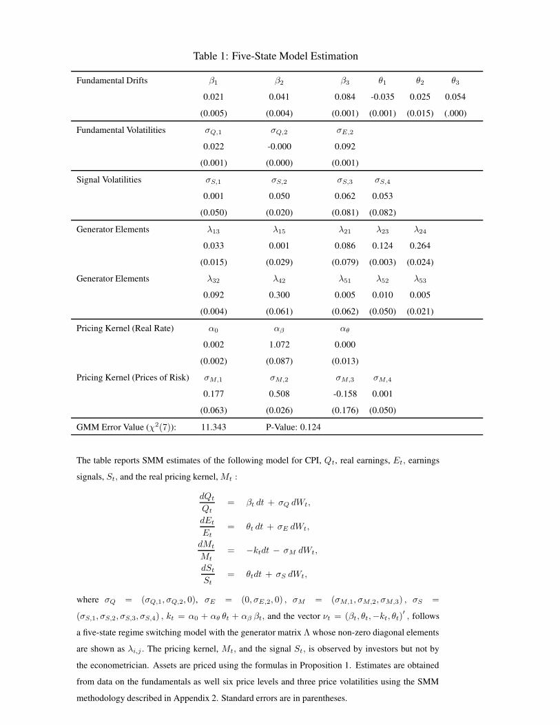
Table 1: Five-State Model Estimation

Fundamental Drifts β1 β2 β3 θ1 θ2 θ3

0.021 0.041 0.084 -0.035 0.025 0.054

(0.005) (0.004) (0.001) (0.001) (0.015) (.000)

Fundamental Volatilities σQ,1 σQ,2 σE,2

0.022 -0.000 0.092

(0.001) (0.000) (0.001)

Signal Volatilities σS,1 σS,2 σS,3 σS,4

0.001 0.050 0.062 0.053

(0.050) (0.020) (0.081) (0.082)

Generator Elements λ13 λ15 λ21 λ23 λ24

0.033 0.001 0.086 0.124 0.264

(0.015) (0.029) (0.079) (0.003) (0.024)

Generator Elements λ32 λ42 λ51 λ52 λ53

0.092 0.300 0.005 0.010 0.005

(0.004) (0.061) (0.062) (0.050) (0.021)

Pricing Kernel (Real Rate) α0 αβ αθ

0.002 1.072 0.000

(0.002) (0.087) (0.013)

Pricing Kernel (Prices of Risk) σM,1 σM,2 σM,3 σM,4

0.177 0.508 -0.158 0.001

(0.063) (0.026) (0.176) (0.050)

GMM Error Value (χ2(7)): 11.343 P-Value: 0.124

The table reports SMM estimates of the following model for CPI, Qt, real earnings, Et, earnings

signals, St, and the real pricing kernel, Mt :

dQt

Qt

= βt dt + σQ dWt,

dEt

Et

= θt dt + σE dWt,

dMt

Mt

= −ktdt − σM dWt,

dSt

St

= θtdt + σS dWt,

where σQ = (σQ,1, σQ,2, 0), σE = (0, σE,2, 0) , σM = (σM,1, σM,2, σM,3) , σS =

(σS,1, σS,2, σS,3, σS,4) , kt = α0 + αθ θt + αβ βt, and the vector νt = (βt, θt,−kt, θt)′

, follows

a five-state regime switching model with the generator matrix Λ whose non-zero diagonal elements

are shown as λi,j . The pricing kernel, Mt, and the signal St, is observed by investors but not by

the econometrician. Assets are priced using the formulas in Proposition 1. Estimates are obtained

from data on the fundamentals as well six price levels and three price volatilities using the SMM

methodology described in Appendix 2. Standard errors are in parentheses.

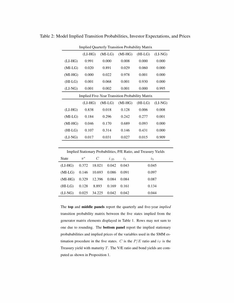
Table 2: Model Implied Transition Probabilities, Investor Expectations, and Prices

Implied Quarterly Transition Probability Matrix

(LI-HG) (MI-LG) (MI-HG) (HI-LG) (LI-NG)

(LI-HG) 0.991 0.000 0.008 0.000 0.000

(MI-LG) 0.020 0.891 0.029 0.060 0.000

(MI-HG) 0.000 0.022 0.978 0.001 0.000

(HI-LG) 0.001 0.068 0.001 0.930 0.000

(LI-NG) 0.001 0.002 0.001 0.000 0.995

Implied Five-Year Transition Probability Matrix

(LI-HG) (MI-LG) (MI-HG) (HI-LG) (LI-NG)

(LI-HG) 0.838 0.018 0.128 0.006 0.008

(MI-LG) 0.184 0.296 0.242 0.277 0.001

(MI-HG) 0.046 0.170 0.689 0.093 0.000

(HI-LG) 0.107 0.314 0.146 0.431 0.000

(LI-NG) 0.017 0.031 0.027 0.015 0.909

Implied Stationary Probabilities, P/E Ratio, and Treasury Yields

State π∗ C i.25 i1 i5

(LI-HG) 0.372 18.021 0.042 0.043 0.045

(MI-LG) 0.146 10.693 0.086 0.091 0.097

(MI-HG) 0.329 12.396 0.084 0.084 0.087

(HI-LG) 0.128 8.893 0.169 0.161 0.134

(LI-NG) 0.025 34.225 0.042 0.042 0.044

The top and middle panels report the quarterly and five-year implied

transition probability matrix between the five states implied from the

generator matrix elements displayed in Table 1. Rows may not sum to

one due to rounding. The bottom panel report the implied stationary

probababilities and implied prices of the variables used in the SMM es-

timation procedure in the five states. C is the P/E ratio and iT is the

Treasury yield with maturity T . The V/E ratio and bond yields are com-

puted as shown in Proposition 1.

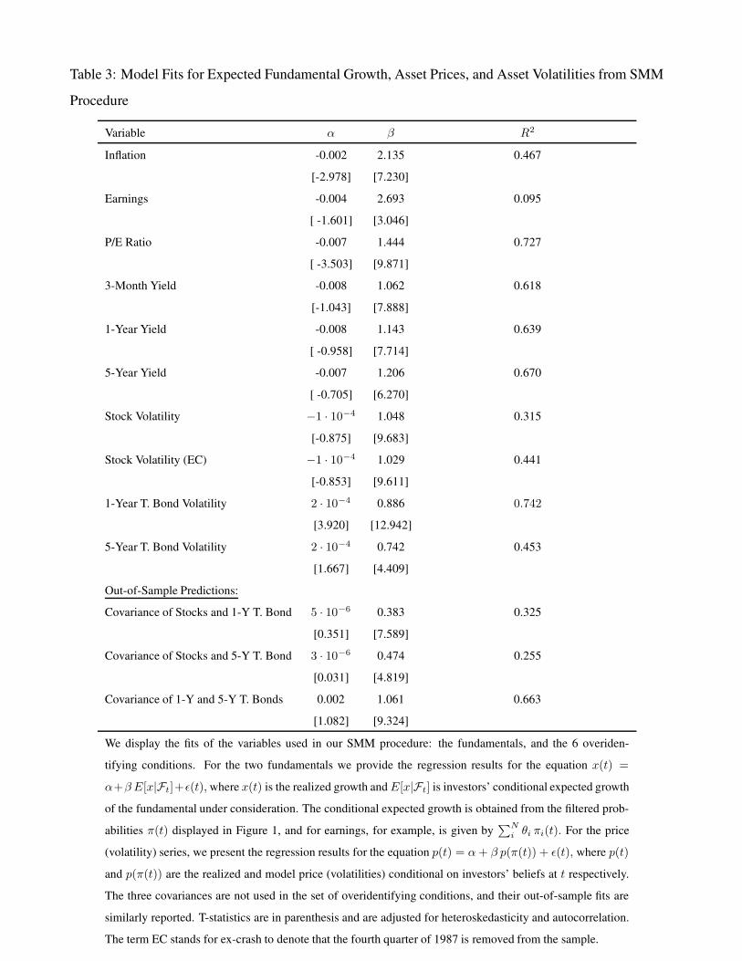
Table 3: Model Fits for Expected Fundamental Growth, Asset Prices, and Asset Volatilities from SMM

Procedure

Variable α β R2

Inflation -0.002 2.135 0.467

[-2.978] [7.230]

Earnings -0.004 2.693 0.095

[ -1.601] [3.046]

P/E Ratio -0.007 1.444 0.727

[ -3.503] [9.871]

3-Month Yield -0.008 1.062 0.618

[-1.043] [7.888]

1-Year Yield -0.008 1.143 0.639

[ -0.958] [7.714]

5-Year Yield -0.007 1.206 0.670

[ -0.705] [6.270]

Stock Volatility −1 · 10−4 1.048 0.315

[-0.875] [9.683]

Stock Volatility (EC) −1 · 10−4 1.029 0.441

[-0.853] [9.611]

1-Year T. Bond Volatility 2 · 10−4 0.886 0.742

[3.920] [12.942]

5-Year T. Bond Volatility 2 · 10−4 0.742 0.453

[1.667] [4.409]

Out-of-Sample Predictions:

Covariance of Stocks and 1-Y T. Bond 5 · 10−6 0.383 0.325

[0.351] [7.589]

Covariance of Stocks and 5-Y T. Bond 3 · 10−6 0.474 0.255

[0.031] [4.819]

Covariance of 1-Y and 5-Y T. Bonds 0.002 1.061 0.663

[1.082] [9.324]

We display the fits of the variables used in our SMM procedure: the fundamentals, and the 6 overiden-

tifying conditions. For the two fundamentals we provide the regression results for the equation x(t) =

α+β E[x|Ft]+ε(t), where x(t) is the realized growth and E[x|Ft] is investors’ conditional expected growth

of the fundamental under consideration. The conditional expected growth is obtained from the filtered prob-

abilities π(t) displayed in Figure 1, and for earnings, for example, is given by∑N

i θi πi(t). For the price

(volatility) series, we present the regression results for the equation p(t) = α + β p(π(t)) + ε(t), where p(t)

and p(π(t)) are the realized and model price (volatilities) conditional on investors’ beliefs at t respectively.

The three covariances are not used in the set of overidentifying conditions, and their out-of-sample fits are

similarly reported. T-statistics are in parenthesis and are adjusted for heteroskedasticity and autocorrelation.

The term EC stands for ex-crash to denote that the fourth quarter of 1987 is removed from the sample.

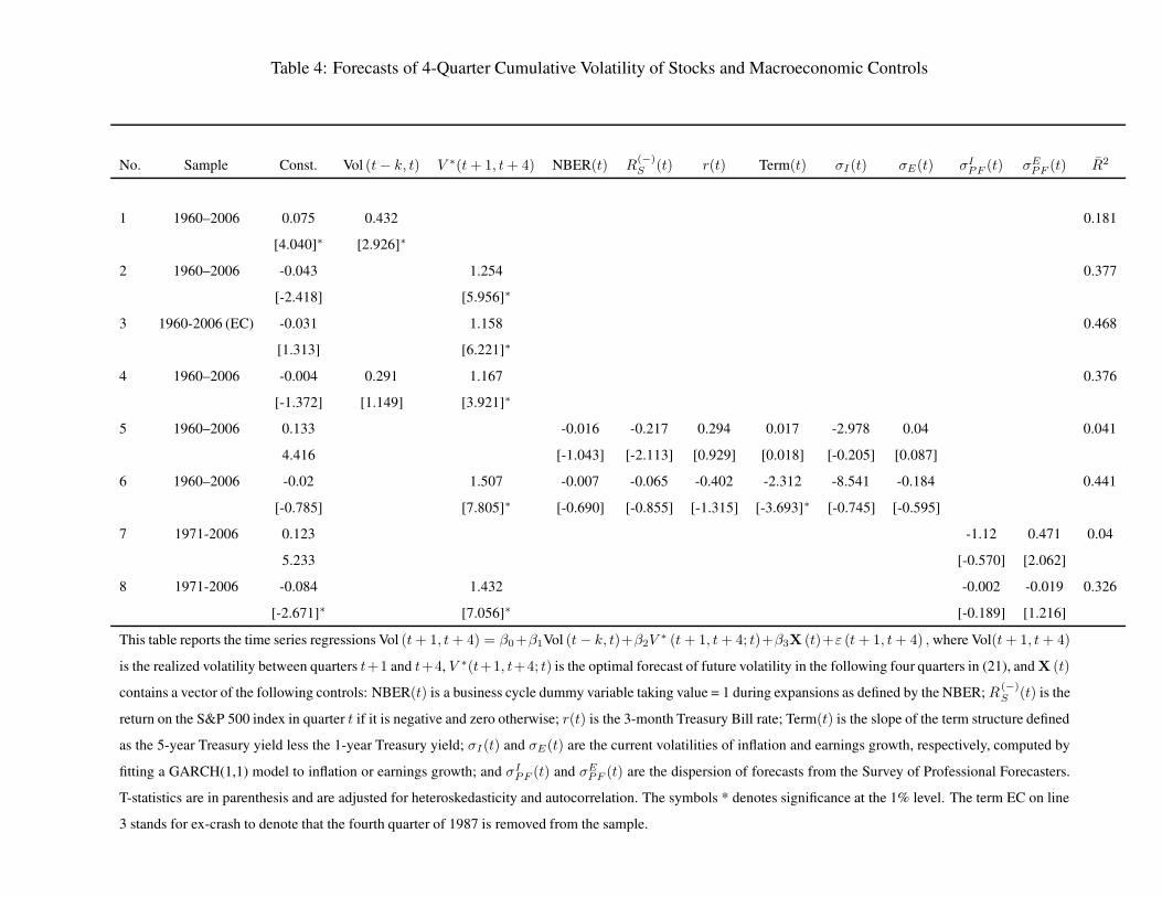
Table 4: Forecasts of 4-Quarter Cumulative Volatility of Stocks and Macroeconomic Controls

No. Sample Const. Vol (t − k, t) V ∗(t + 1, t + 4) NBER(t) R(−)S (t) r(t) Term(t) σI (t) σE(t) σI

PF (t) σEPF (t) R2

1 1960–2006 0.075 0.432 0.181

[4.040]∗ [2.926]∗

2 1960–2006 -0.043 1.254 0.377

[-2.418] [5.956]∗

3 1960-2006 (EC) -0.031 1.158 0.468

[1.313] [6.221]∗

4 1960–2006 -0.004 0.291 1.167 0.376

[-1.372] [1.149] [3.921]∗

5 1960–2006 0.133 -0.016 -0.217 0.294 0.017 -2.978 0.04 0.041

4.416 [-1.043] [-2.113] [0.929] [0.018] [-0.205] [0.087]

6 1960–2006 -0.02 1.507 -0.007 -0.065 -0.402 -2.312 -8.541 -0.184 0.441

[-0.785] [7.805]∗ [-0.690] [-0.855] [-1.315] [-3.693]∗ [-0.745] [-0.595]

7 1971-2006 0.123 -1.12 0.471 0.04

5.233 [-0.570] [2.062]

8 1971-2006 -0.084 1.432 -0.002 -0.019 0.326

[-2.671]∗ [7.056]∗ [-0.189] [1.216]

This table reports the time series regressions Vol (t + 1, t + 4) = β0+β1Vol (t − k, t)+β2V∗ (t + 1, t + 4; t)+β3X (t)+ε (t + 1, t + 4) , where Vol(t + 1, t + 4)

is the realized volatility between quarters t+1 and t+4, V ∗(t+1, t+4; t) is the optimal forecast of future volatility in the following four quarters in (21), and X (t)

contains a vector of the following controls: NBER(t) is a business cycle dummy variable taking value = 1 during expansions as defined by the NBER; R(−)S (t) is the

return on the S&P 500 index in quarter t if it is negative and zero otherwise; r(t) is the 3-month Treasury Bill rate; Term(t) is the slope of the term structure defined

as the 5-year Treasury yield less the 1-year Treasury yield; σI (t) and σE(t) are the current volatilities of inflation and earnings growth, respectively, computed by

fitting a GARCH(1,1) model to inflation or earnings growth; and σIPF (t) and σE

PF (t) are the dispersion of forecasts from the Survey of Professional Forecasters.

T-statistics are in parenthesis and are adjusted for heteroskedasticity and autocorrelation. The symbols * denotes significance at the 1% level. The term EC on line

3 stands for ex-crash to denote that the fourth quarter of 1987 is removed from the sample.

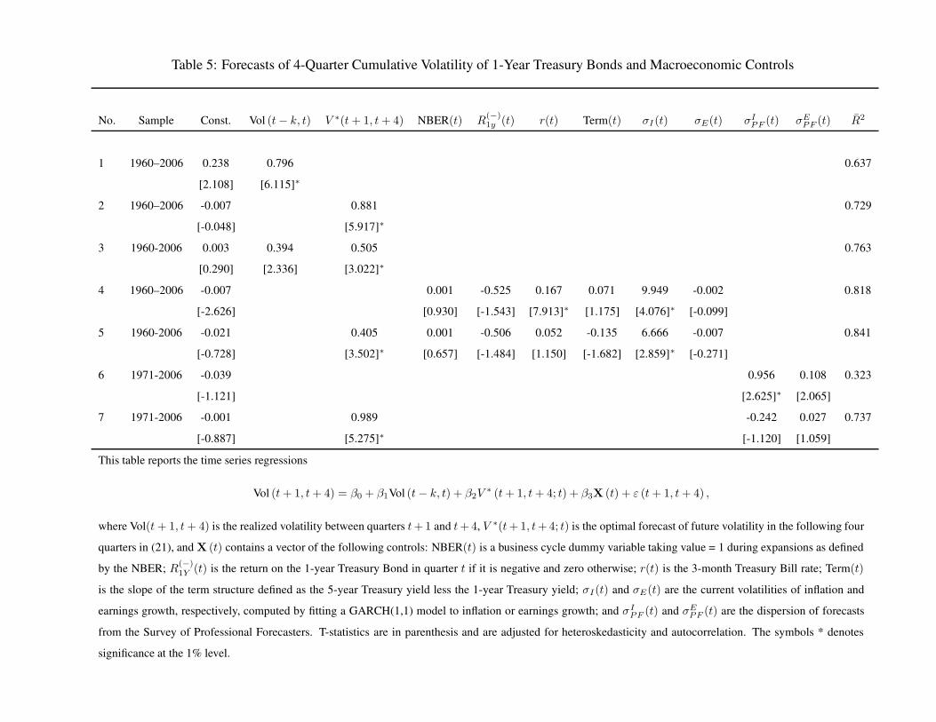
Table 5: Forecasts of 4-Quarter Cumulative Volatility of 1-Year Treasury Bonds and Macroeconomic Controls

No. Sample Const. Vol (t − k, t) V ∗(t + 1, t + 4) NBER(t) R(−)1y (t) r(t) Term(t) σI (t) σE(t) σI

PF (t) σEPF (t) R2

1 1960–2006 0.238 0.796 0.637

[2.108] [6.115]∗

2 1960–2006 -0.007 0.881 0.729

[-0.048] [5.917]∗

3 1960-2006 0.003 0.394 0.505 0.763

[0.290] [2.336] [3.022]∗

4 1960–2006 -0.007 0.001 -0.525 0.167 0.071 9.949 -0.002 0.818

[-2.626] [0.930] [-1.543] [7.913]∗ [1.175] [4.076]∗ [-0.099]

5 1960-2006 -0.021 0.405 0.001 -0.506 0.052 -0.135 6.666 -0.007 0.841

[-0.728] [3.502]∗ [0.657] [-1.484] [1.150] [-1.682] [2.859]∗ [-0.271]

6 1971-2006 -0.039 0.956 0.108 0.323

[-1.121] [2.625]∗ [2.065]

7 1971-2006 -0.001 0.989 -0.242 0.027 0.737

[-0.887] [5.275]∗ [-1.120] [1.059]

This table reports the time series regressions

Vol (t + 1, t + 4) = β0 + β1Vol (t − k, t) + β2V∗ (t + 1, t + 4; t) + β3X (t) + ε (t + 1, t + 4) ,

where Vol(t + 1, t + 4) is the realized volatility between quarters t + 1 and t + 4, V ∗(t + 1, t + 4; t) is the optimal forecast of future volatility in the following four

quarters in (21), and X (t) contains a vector of the following controls: NBER(t) is a business cycle dummy variable taking value = 1 during expansions as defined

by the NBER; R(−)1Y (t) is the return on the 1-year Treasury Bond in quarter t if it is negative and zero otherwise; r(t) is the 3-month Treasury Bill rate; Term(t)

is the slope of the term structure defined as the 5-year Treasury yield less the 1-year Treasury yield; σI(t) and σE(t) are the current volatilities of inflation and

earnings growth, respectively, computed by fitting a GARCH(1,1) model to inflation or earnings growth; and σIPF (t) and σE

PF (t) are the dispersion of forecasts

from the Survey of Professional Forecasters. T-statistics are in parenthesis and are adjusted for heteroskedasticity and autocorrelation. The symbols * denotes

significance at the 1% level.

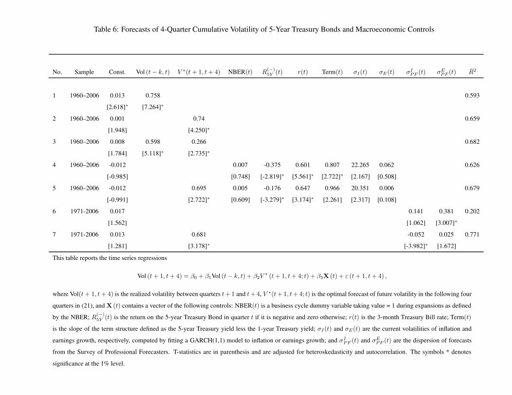
Table 6: Forecasts of 4-Quarter Cumulative Volatility of 5-Year Treasury Bonds and Macroeconomic Controls

No. Sample Const. Vol (t − k, t) V ∗(t + 1, t + 4) NBER(t) R(−)5Y (t) r(t) Term(t) σI(t) σE(t) σI

PF (t) σEPF (t) R2

1 1960–2006 0.013 0.758 0.593

[2.618]∗ [7.264]∗

2 1960–2006 0.001 0.74 0.659

[1.948] [4.250]∗

3 1960–2006 0.008 0.598 0.266 0.682

[1.784] [5.118]∗ [2.735]∗

4 1960–2006 -0.012 0.007 -0.375 0.601 0.807 22.265 0.062 0.626

[-0.985] [0.748] [-2.819]∗ [5.561]∗ [2.722]∗ [2.167] [0.508]

5 1960–2006 -0.012 0.695 0.005 -0.176 0.647 0.966 20.351 0.006 0.679

[-0.991] [2.722]∗ [0.609] [-3.279]∗ [3.174]∗ [2.261] [2.317] [0.108]

6 1971-2006 0.017 0.141 0.381 0.202

[1.562] [1.062] [3.007]∗

7 1971-2006 0.013 0.681 -0.052 0.025 0.771

[1.281] [3.178]∗ [-3.982]∗ [1.672]

This table reports the time series regressions

Vol (t + 1, t + 4) = β0 + β1Vol (t − k, t) + β2V∗ (t + 1, t + 4; t) + β3X (t) + ε (t + 1, t + 4) ,

where Vol(t + 1, t + 4) is the realized volatility between quarters t + 1 and t + 4, V ∗(t + 1, t + 4; t) is the optimal forecast of future volatility in the following four

quarters in (21), and X (t) contains a vector of the following controls: NBER(t) is a business cycle dummy variable taking value = 1 during expansions as defined

by the NBER; R(−)5Y (t) is the return on the 5-year Treasury Bond in quarter t if it is negative and zero otherwise; r(t) is the 3-month Treasury Bill rate; Term(t)

is the slope of the term structure defined as the 5-year Treasury yield less the 1-year Treasury yield; σI(t) and σE(t) are the current volatilities of inflation and

earnings growth, respectively, computed by fitting a GARCH(1,1) model to inflation or earnings growth; and σIPF (t) and σE

PF (t) are the dispersion of forecasts

from the Survey of Professional Forecasters. T-statistics are in parenthesis and are adjusted for heteroskedasticity and autocorrelation. The symbols * denotes

significance at the 1% level.

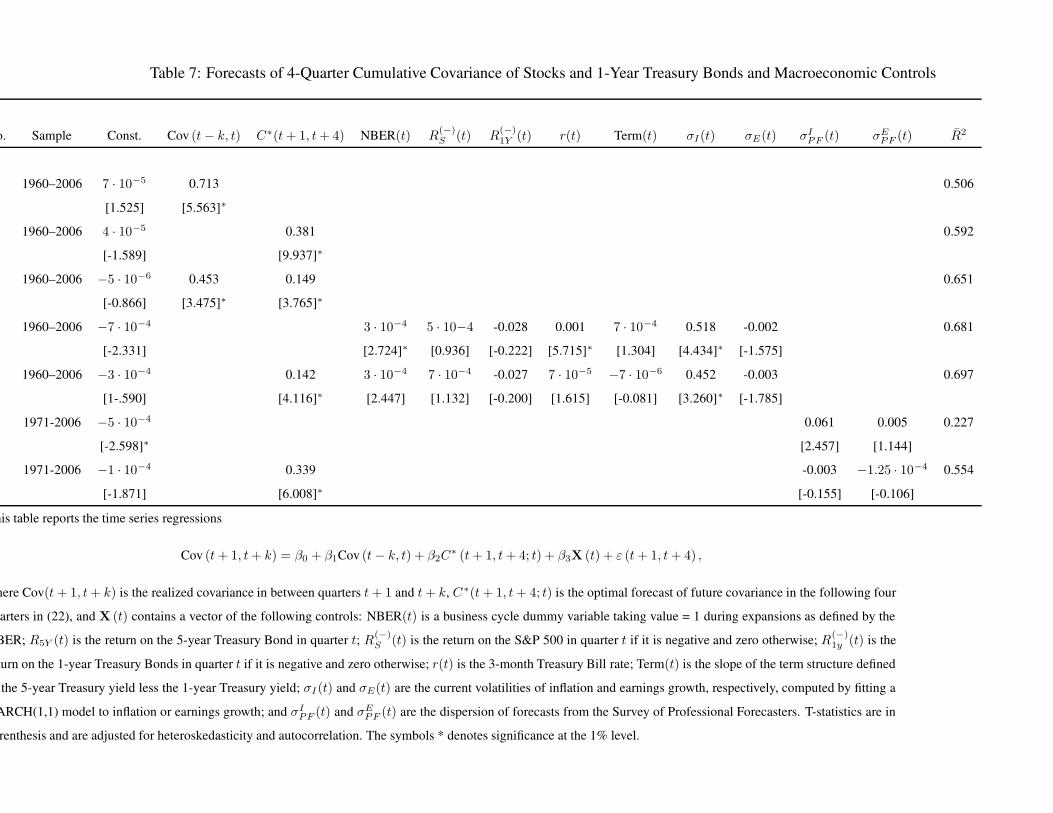
Table 7: Forecasts of 4-Quarter Cumulative Covariance of Stocks and 1-Year Treasury Bonds and Macroeconomic Controls

No. Sample Const. Cov (t − k, t) C∗(t + 1, t + 4) NBER(t) R(−)S (t) R

(−)1Y (t) r(t) Term(t) σI(t) σE(t) σI

PF (t) σEPF (t) R2

1 1960–2006 7 · 10−5 0.713 0.506

[1.525] [5.563]∗

2 1960–2006 4 · 10−5 0.381 0.592

[-1.589] [9.937]∗

3 1960–2006 −5 · 10−6 0.453 0.149 0.651

[-0.866] [3.475]∗ [3.765]∗

4 1960–2006 −7 · 10−4 3 · 10−4 5 · 10−4 -0.028 0.001 7 · 10−4 0.518 -0.002 0.681

[-2.331] [2.724]∗ [0.936] [-0.222] [5.715]∗ [1.304] [4.434]∗ [-1.575]

5 1960–2006 −3 · 10−4 0.142 3 · 10−4 7 · 10−4 -0.027 7 · 10−5 −7 · 10−6 0.452 -0.003 0.697

[1-.590] [4.116]∗ [2.447] [1.132] [-0.200] [1.615] [-0.081] [3.260]∗ [-1.785]

6 1971-2006 −5 · 10−4 0.061 0.005 0.227

[-2.598]∗ [2.457] [1.144]

7 1971-2006 −1 · 10−4 0.339 -0.003 −1.25 · 10−4 0.554

[-1.871] [6.008]∗ [-0.155] [-0.106]

This table reports the time series regressions

Cov (t + 1, t + k) = β0 + β1Cov (t − k, t) + β2C∗ (t + 1, t + 4; t) + β3X (t) + ε (t + 1, t + 4) ,

where Cov(t + 1, t + k) is the realized covariance in between quarters t + 1 and t + k, C∗(t + 1, t + 4; t) is the optimal forecast of future covariance in the following four

quarters in (22), and X (t) contains a vector of the following controls: NBER(t) is a business cycle dummy variable taking value = 1 during expansions as defined by the

NBER; R5Y (t) is the return on the 5-year Treasury Bond in quarter t; R(−)S (t) is the return on the S&P 500 in quarter t if it is negative and zero otherwise; R

(−)1y (t) is the

return on the 1-year Treasury Bonds in quarter t if it is negative and zero otherwise; r(t) is the 3-month Treasury Bill rate; Term(t) is the slope of the term structure defined

as the 5-year Treasury yield less the 1-year Treasury yield; σI (t) and σE(t) are the current volatilities of inflation and earnings growth, respectively, computed by fitting a

GARCH(1,1) model to inflation or earnings growth; and σIPF (t) and σE

PF (t) are the dispersion of forecasts from the Survey of Professional Forecasters. T-statistics are in

parenthesis and are adjusted for heteroskedasticity and autocorrelation. The symbols * denotes significance at the 1% level.

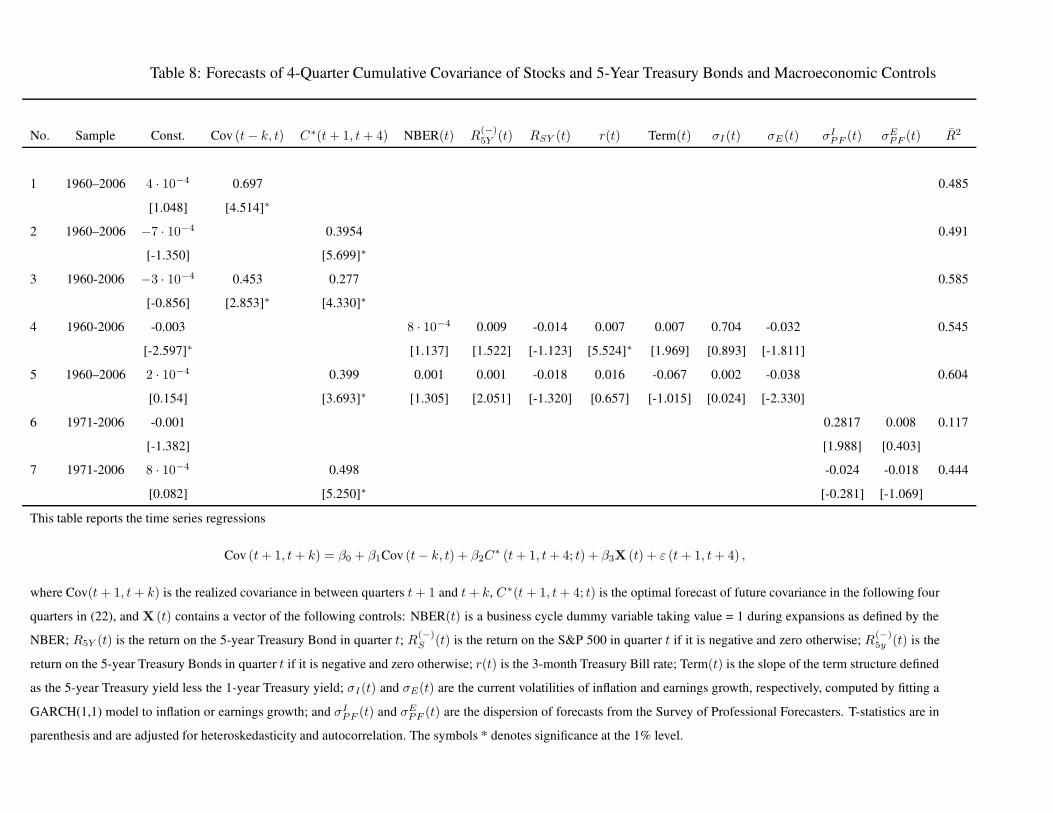
Table 8: Forecasts of 4-Quarter Cumulative Covariance of Stocks and 5-Year Treasury Bonds and Macroeconomic Controls

No. Sample Const. Cov (t − k, t) C∗(t + 1, t + 4) NBER(t) R(−)5Y (t) RSY (t) r(t) Term(t) σI (t) σE(t) σI

PF (t) σEPF (t) R2

1 1960–2006 4 · 10−4 0.697 0.485

[1.048] [4.514]∗

2 1960–2006 −7 · 10−4 0.3954 0.491

[-1.350] [5.699]∗

3 1960-2006 −3 · 10−4 0.453 0.277 0.585

[-0.856] [2.853]∗ [4.330]∗

4 1960-2006 -0.003 8 · 10−4 0.009 -0.014 0.007 0.007 0.704 -0.032 0.545

[-2.597]∗ [1.137] [1.522] [-1.123] [5.524]∗ [1.969] [0.893] [-1.811]

5 1960–2006 2 · 10−4 0.399 0.001 0.001 -0.018 0.016 -0.067 0.002 -0.038 0.604

[0.154] [3.693]∗ [1.305] [2.051] [-1.320] [0.657] [-1.015] [0.024] [-2.330]

6 1971-2006 -0.001 0.2817 0.008 0.117

[-1.382] [1.988] [0.403]

7 1971-2006 8 · 10−4 0.498 -0.024 -0.018 0.444

[0.082] [5.250]∗ [-0.281] [-1.069]

This table reports the time series regressions

Cov (t + 1, t + k) = β0 + β1Cov (t − k, t) + β2C∗ (t + 1, t + 4; t) + β3X (t) + ε (t + 1, t + 4) ,

where Cov(t + 1, t + k) is the realized covariance in between quarters t + 1 and t + k, C∗(t + 1, t + 4; t) is the optimal forecast of future covariance in the following four

quarters in (22), and X (t) contains a vector of the following controls: NBER(t) is a business cycle dummy variable taking value = 1 during expansions as defined by the

NBER; R5Y (t) is the return on the 5-year Treasury Bond in quarter t; R(−)S (t) is the return on the S&P 500 in quarter t if it is negative and zero otherwise; R

(−)5y (t) is the

return on the 5-year Treasury Bonds in quarter t if it is negative and zero otherwise; r(t) is the 3-month Treasury Bill rate; Term(t) is the slope of the term structure defined

as the 5-year Treasury yield less the 1-year Treasury yield; σI(t) and σE(t) are the current volatilities of inflation and earnings growth, respectively, computed by fitting a

GARCH(1,1) model to inflation or earnings growth; and σIPF (t) and σE

PF (t) are the dispersion of forecasts from the Survey of Professional Forecasters. T-statistics are in

parenthesis and are adjusted for heteroskedasticity and autocorrelation. The symbols * denotes significance at the 1% level.

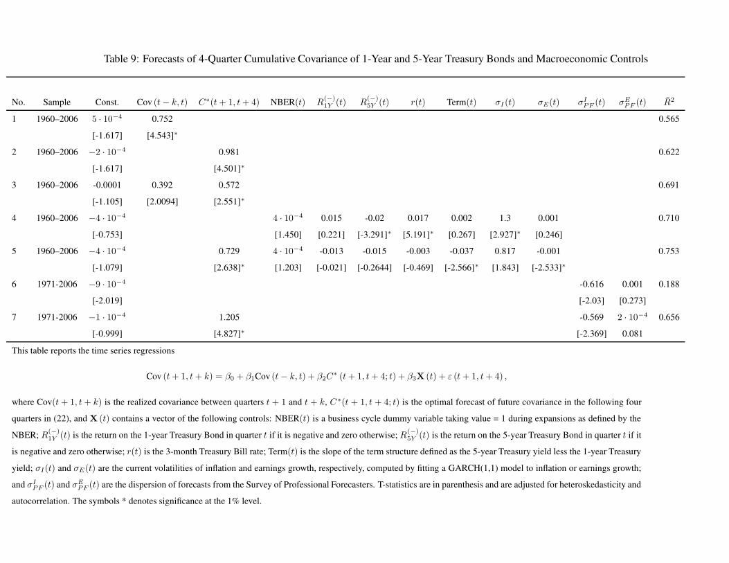
Table 9: Forecasts of 4-Quarter Cumulative Covariance of 1-Year and 5-Year Treasury Bonds and Macroeconomic Controls

No. Sample Const. Cov (t − k, t) C∗(t + 1, t + 4) NBER(t) R(−)1Y (t) R

(−)5Y (t) r(t) Term(t) σI (t) σE(t) σI

PF (t) σEPF (t) R2

1 1960–2006 5 · 10−4 0.752 0.565

[-1.617] [4.543]∗

2 1960–2006 −2 · 10−4 0.981 0.622

[-1.617] [4.501]∗

3 1960–2006 -0.0001 0.392 0.572 0.691

[-1.105] [2.0094] [2.551]∗

4 1960–2006 −4 · 10−4 4 · 10−4 0.015 -0.02 0.017 0.002 1.3 0.001 0.710

[-0.753] [1.450] [0.221] [-3.291]∗ [5.191]∗ [0.267] [2.927]∗ [0.246]

5 1960–2006 −4 · 10−4 0.729 4 · 10−4 -0.013 -0.015 -0.003 -0.037 0.817 -0.001 0.753

[-1.079] [2.638]∗ [1.203] [-0.021] [-0.2644] [-0.469] [-2.566]∗ [1.843] [-2.533]∗

6 1971-2006 −9 · 10−4 -0.616 0.001 0.188

[-2.019] [-2.03] [0.273]

7 1971-2006 −1 · 10−4 1.205 -0.569 2 · 10−4 0.656

[-0.999] [4.827]∗ [-2.369] 0.081

This table reports the time series regressions

Cov (t + 1, t + k) = β0 + β1Cov (t − k, t) + β2C∗ (t + 1, t + 4; t) + β3X (t) + ε (t + 1, t + 4) ,

where Cov(t + 1, t + k) is the realized covariance between quarters t + 1 and t + k, C∗(t + 1, t + 4; t) is the optimal forecast of future covariance in the following four

quarters in (22), and X (t) contains a vector of the following controls: NBER(t) is a business cycle dummy variable taking value = 1 during expansions as defined by the

NBER; R(−)1Y (t) is the return on the 1-year Treasury Bond in quarter t if it is negative and zero otherwise; R

(−)5Y (t) is the return on the 5-year Treasury Bond in quarter t if it

is negative and zero otherwise; r(t) is the 3-month Treasury Bill rate; Term(t) is the slope of the term structure defined as the 5-year Treasury yield less the 1-year Treasury

yield; σI(t) and σE(t) are the current volatilities of inflation and earnings growth, respectively, computed by fitting a GARCH(1,1) model to inflation or earnings growth;

and σIPF (t) and σE

PF (t) are the dispersion of forecasts from the Survey of Professional Forecasters. T-statistics are in parenthesis and are adjusted for heteroskedasticity and

autocorrelation. The symbols * denotes significance at the 1% level.

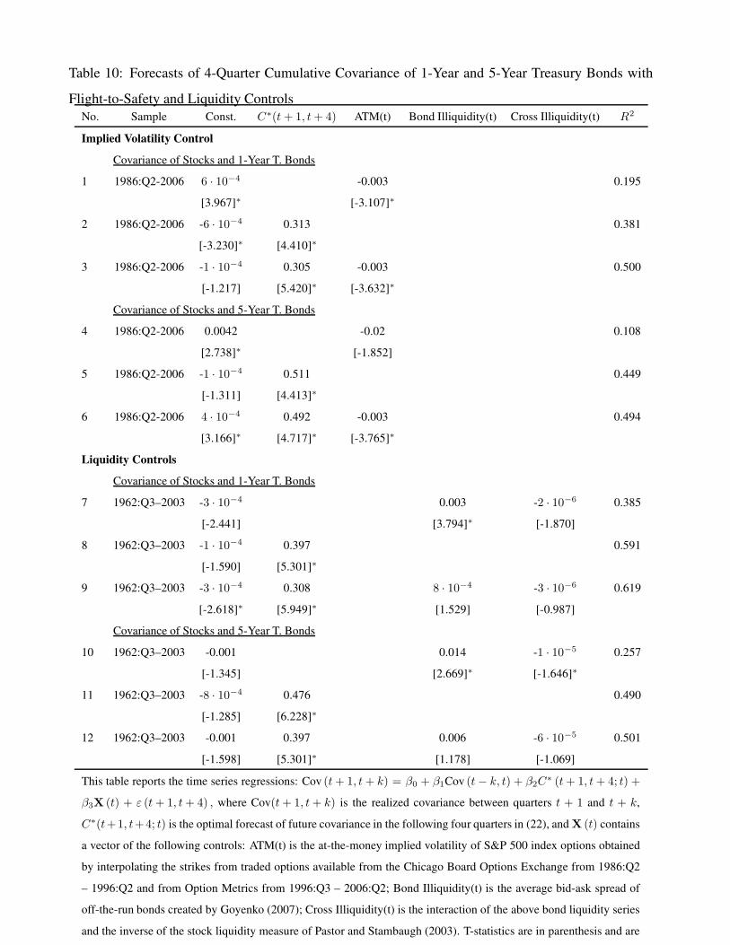
Table 10: Forecasts of 4-Quarter Cumulative Covariance of 1-Year and 5-Year Treasury Bonds with

Flight-to-Safety and Liquidity ControlsNo. Sample Const. C∗(t + 1, t + 4) ATM(t) Bond Illiquidity(t) Cross Illiquidity(t) R2

Implied Volatility ControlCovariance of Stocks and 1-Year T. Bonds

1 1986:Q2-2006 6 · 10−4 -0.003 0.195

[3.967]∗ [-3.107]∗

2 1986:Q2-2006 -6 · 10−4 0.313 0.381

[-3.230]∗ [4.410]∗

3 1986:Q2-2006 -1 · 10−4 0.305 -0.003 0.500

[-1.217] [5.420]∗ [-3.632]∗

Covariance of Stocks and 5-Year T. Bonds

4 1986:Q2-2006 0.0042 -0.02 0.108

[2.738]∗ [-1.852]

5 1986:Q2-2006 -1 · 10−4 0.511 0.449

[-1.311] [4.413]∗

6 1986:Q2-2006 4 · 10−4 0.492 -0.003 0.494

[3.166]∗ [4.717]∗ [-3.765]∗

Liquidity ControlsCovariance of Stocks and 1-Year T. Bonds

7 1962:Q3–2003 -3 · 10−4 0.003 -2 · 10−6 0.385

[-2.441] [3.794]∗ [-1.870]

8 1962:Q3–2003 -1 · 10−4 0.397 0.591

[-1.590] [5.301]∗

9 1962:Q3–2003 -3 · 10−4 0.308 8 · 10−4 -3 · 10−6 0.619

[-2.618]∗ [5.949]∗ [1.529] [-0.987]

Covariance of Stocks and 5-Year T. Bonds

10 1962:Q3–2003 -0.001 0.014 -1 · 10−5 0.257

[-1.345] [2.669]∗ [-1.646]∗

11 1962:Q3–2003 -8 · 10−4 0.476 0.490

[-1.285] [6.228]∗

12 1962:Q3–2003 -0.001 0.397 0.006 -6 · 10−5 0.501

[-1.598] [5.301]∗ [1.178] [-1.069]

This table reports the time series regressions: Cov (t + 1, t + k) = β0 + β1Cov (t − k, t) + β2C∗ (t + 1, t + 4; t) +

β3X (t) + ε (t + 1, t + 4) , where Cov(t + 1, t + k) is the realized covariance between quarters t + 1 and t + k,

C∗(t+1, t+4; t) is the optimal forecast of future covariance in the following four quarters in (22), and X (t) contains

a vector of the following controls: ATM(t) is the at-the-money implied volatility of S&P 500 index options obtained

by interpolating the strikes from traded options available from the Chicago Board Options Exchange from 1986:Q2

– 1996:Q2 and from Option Metrics from 1996:Q3 – 2006:Q2; Bond Illiquidity(t) is the average bid-ask spread of

off-the-run bonds created by Goyenko (2007); Cross Illiquidity(t) is the interaction of the above bond liquidity series

and the inverse of the stock liquidity measure of Pastor and Stambaugh (2003). T-statistics are in parenthesis and are

adjusted for heteroskedasticity and autocorrelation. The symbols * denotes significance at the 1% level.

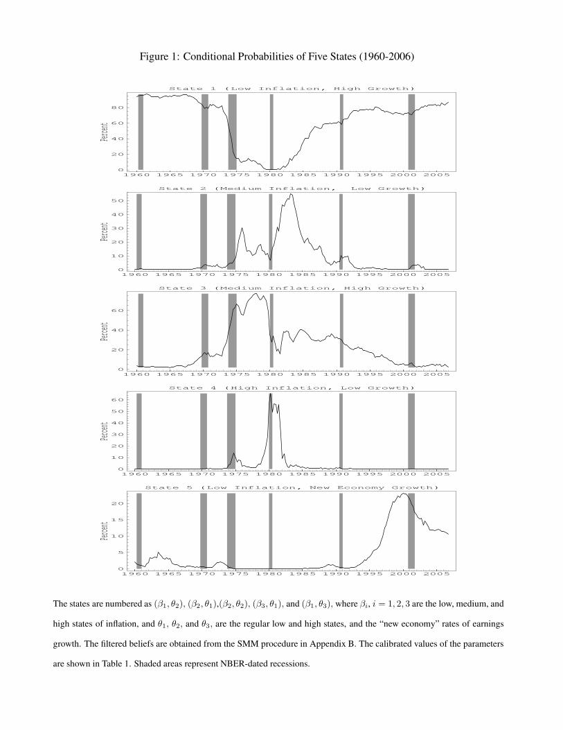
Figure 1: Conditional Probabilities of Five States (1960-2006)

1960

1965

1970

1975

1980

1985

1990

1995

2000

2005 0

5

10

15

20

Percen

t

State 5 (Low Inflation, New Economy Growth)

1960

1965

1970

1975

1980

1985

1990

1995

2000

2005 0

10

20

30

40

50

60

Percen

t

State 4 (High Inflation, Low Growth)

1960

1965

1970

1975

1980

1985

1990

1995

2000

2005 0

20

40

60

Percen

t

State 3 (Medium Inflation, High Growth)

1960

1965

1970

1975

1980

1985

1990

1995

2000

2005 0

10

20

30

40

50

Percen

t

State 2 (Medium Inflation, Low Growth)

1960

1965

1970

1975

1980

1985

1990

1995

2000

2005 0

20

40

60

80Per

cent

State 1 (Low Inflation, High Growth)

The states are numbered as (β1, θ2), (β2, θ1),(β2, θ2), (β3, θ1), and (β1, θ3), where βi, i = 1, 2, 3 are the low, medium, and

high states of inflation, and θ1, θ2, and θ3, are the regular low and high states, and the “new economy” rates of earnings

growth. The filtered beliefs are obtained from the SMM procedure in Appendix B. The calibrated values of the parameters

are shown in Table 1. Shaded areas represent NBER-dated recessions.

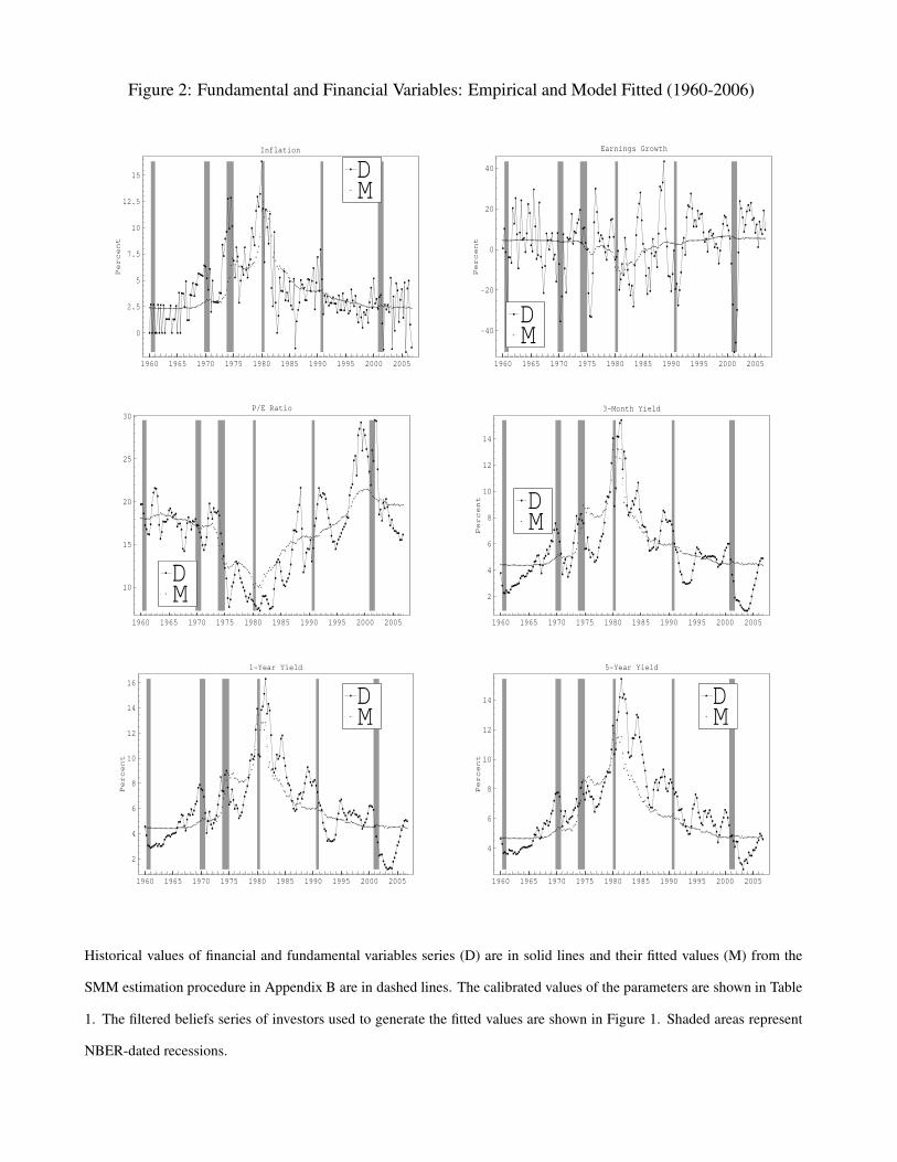
Figure 2: Fundamental and Financial Variables: Empirical and Model Fitted (1960-2006)

1960

1965

1970

1975

1980

1985

1990

1995

2000

2005

2

4

6

8

10

12

14

16

Percent

1-Year Yield

MD

1960

1965

1970

1975

1980

1985

1990

1995

2000

2005

4

6

8

10

12

14

Percent

5-Year Yield

MD

1960

1965

1970

1975

1980

1985

1990

1995

2000

2005

10

15

20

25

30P/E Ratio

MD

1960

1965

1970

1975

1980

1985

1990

1995

2000

2005

2

4

6

8

10

12

14

Percent

3-Month Yield

MD

1960

1965

1970

1975

1980

1985

1990

1995

2000

2005

0

2.5

5

7.5

10

12.5

15

Percent

Inflation

MD

1960

1965

1970

1975

1980

1985

1990

1995

2000

2005

-40

-20

0

20

40

Percent

Earnings Growth

MD

Historical values of financial and fundamental variables series (D) are in solid lines and their fitted values (M) from the

SMM estimation procedure in Appendix B are in dashed lines. The calibrated values of the parameters are shown in Table

1. The filtered beliefs series of investors used to generate the fitted values are shown in Figure 1. Shaded areas represent

NBER-dated recessions.

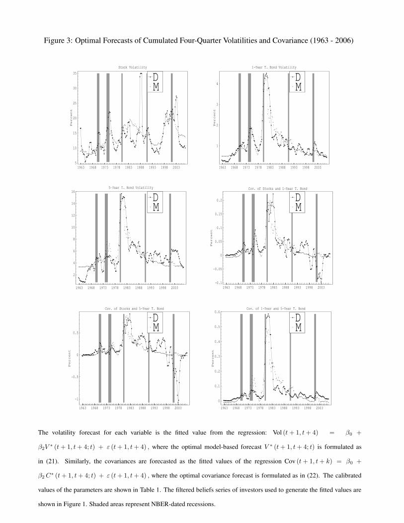
Figure 3: Optimal Forecasts of Cumulated Four-Quarter Volatilities and Covariance (1963 - 2006)

1963

1968

1973

1978

1983

1988

1993

1998

2003

-1

-0.5

0

0.5

Percent

Cov. of Stocks and 5-Year T. Bond

MD

1963

1968

1973

1978

1983

1988

1993

1998

2003

0

0.1

0.2

0.3

0.4

0.5

0.6

Percent

Cov. of 1-Year and 5-Year T. Bond

MD

1963

1968

1973

1978

1983

1988

1993

1998

2003

2

4

6

8

10

12

14

165-Year T. Bond Volatility

MD

1963

1968

1973

1978

1983

1988

1993

1998

2003 -0.1

-0.05

0

0.05

0.1

0.15

0.2

Percent

Cov. of Stocks and 1-Year T. Bond

MD

1963

1968

1973

1978

1983

1988

1993

1998

2003 5

10

15

20

25

30

35Percent

Stock Volatility

MD

1963

1968

1973

1978

1983

1988

1993

1998

2003

1

2

3

4

Percent

1-Year T. Bond Volatility

MD

The volatility forecast for each variable is the fitted value from the regression: Vol (t + 1, t + 4) = β0 +

β2V∗ (t + 1, t + 4; t) + ε (t + 1, t + 4) , where the optimal model-based forecast V ∗ (t + 1, t + 4; t) is formulated as

in (21). Similarly, the covariances are forecasted as the fitted values of the regression Cov (t + 1, t + k) = β0 +

β2 C∗ (t + 1, t + 4; t) + ε (t + 1, t + 4) , where the optimal covariance forecast is formulated as in (22). The calibrated

values of the parameters are shown in Table 1. The filtered beliefs series of investors used to generate the fitted values are

shown in Figure 1. Shaded areas represent NBER-dated recessions.

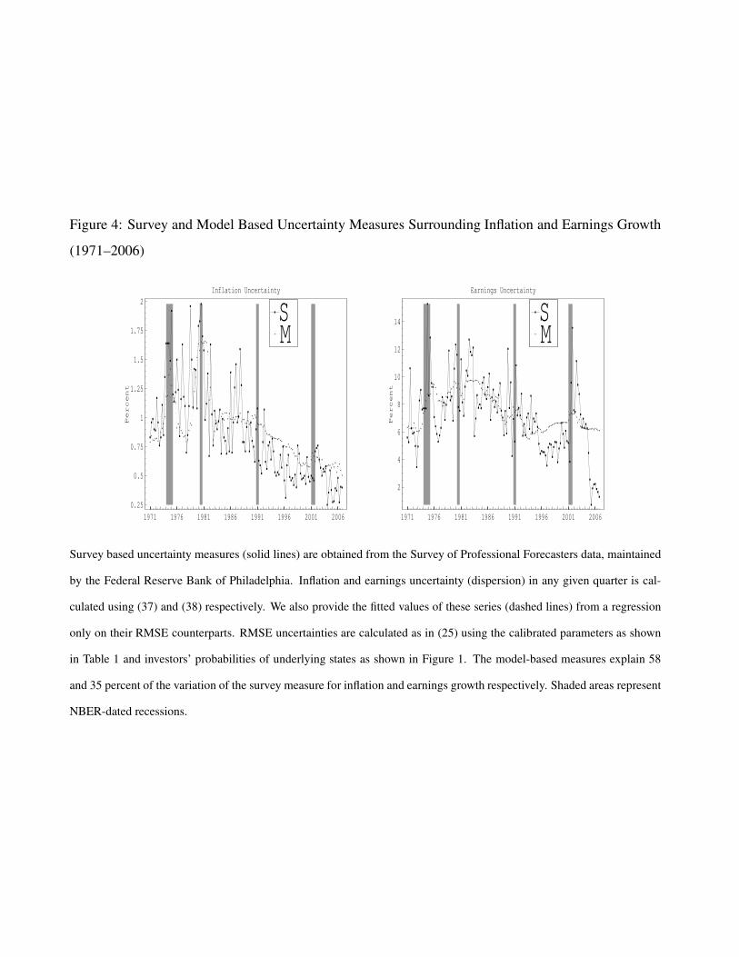
Figure 4: Survey and Model Based Uncertainty Measures Surrounding Inflation and Earnings Growth

(1971–2006)

1971

1976

1981

1986

1991

1996

2001

2006

0.25

0.5

0.75

1

1.25

1.5

1.75

2

Percent

Inflation Uncertainty

MS

1971

1976

1981

1986

1991

1996

2001

2006

2

4

6

8

10

12

14

Percent

Earnings Uncertainty

MS

Survey based uncertainty measures (solid lines) are obtained from the Survey of Professional Forecasters data, maintained

by the Federal Reserve Bank of Philadelphia. Inflation and earnings uncertainty (dispersion) in any given quarter is cal-

culated using (37) and (38) respectively. We also provide the fitted values of these series (dashed lines) from a regression

only on their RMSE counterparts. RMSE uncertainties are calculated as in (25) using the calibrated parameters as shown

in Table 1 and investors’ probabilities of underlying states as shown in Figure 1. The model-based measures explain 58

and 35 percent of the variation of the survey measure for inflation and earnings growth respectively. Shaded areas represent

NBER-dated recessions.

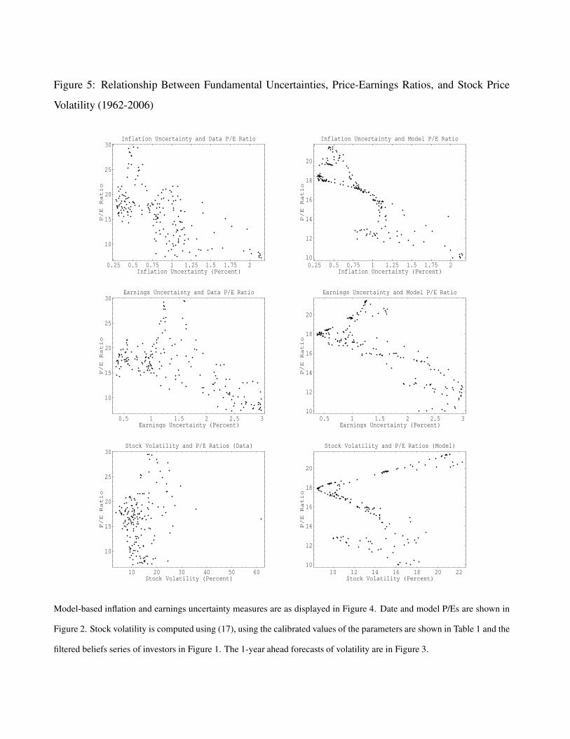
Figure 5: Relationship Between Fundamental Uncertainties, Price-Earnings Ratios, and Stock Price

Volatility (1962-2006)

10 20 30 40 50 60Stock Volatility (Percent)

10

15

20

25

30

P/E Ratio

Stock Volatility and P/E Ratios (Data)

10 12 14 16 18 20 22Stock Volatility (Percent)

10

12

14

16

18

20

P/E Ratio

Stock Volatility and P/E Ratios (Model)

0.5 1 1.5 2 2.5 3Earnings Uncertainty (Percent)

10

15

20

25

30

P/E Ratio

Earnings Uncertainty and Data P/E Ratio

0.5 1 1.5 2 2.5 3Earnings Uncertainty (Percent)

10

12

14

16

18

20

P/E Ratio

Earnings Uncertainty and Model P/E Ratio

0.25 0.5 0.75 1 1.25 1.5 1.75 2Inflation Uncertainty (Percent)

10

15

20

25

30

P/E Ratio

Inflation Uncertainty and Data P/E Ratio

0.25 0.5 0.75 1 1.25 1.5 1.75 2Inflation Uncertainty (Percent)

10

12

14

16

18

20

P/E Ratio

Inflation Uncertainty and Model P/E Ratio

Model-based inflation and earnings uncertainty measures are as displayed in Figure 4. Date and model P/Es are shown in

Figure 2. Stock volatility is computed using (17), using the calibrated values of the parameters are shown in Table 1 and the

filtered beliefs series of investors in Figure 1. The 1-year ahead forecasts of volatility are in Figure 3.

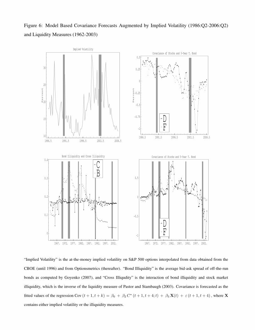
Figure 6: Model Based Covariance Forecasts Augmented by Implied Volatility (1986:Q2-2006:Q2)

and Liquidity Measures (1962-2003)

1967.

1972.

1977.

1982.

1987.

1992.

1997.

2002.

0

0.1

0.2

0.3

0.4Bond Illiquidity and Cross Illiquidity

BC

1967.

1972.

1977.

1982.

1987.

1992.

1997.

2002.

-1

-0.5

0

0.5

Covariance of Stocks and 5-Year T. Bond

FD

1986.5

1991.5

1996.5

2001.5

2006.510

15

20

25

30

Percent

Implied Volatility

1986.5

1991.5

1996.5

2001.5

2006.5

-1

-0.75

-0.5

-0.25

0

0.25

0.5

Percent

Covariance of Stocks and 5-Year T. Bond

FD

“Implied Volatility” is the at-the-money implied volatility on S&P 500 options interpolated from data obtained from the

CBOE (until 1996) and from Optionsmetrics (thereafter). “Bond Illiquidity” is the average bid-ask spread of off-the-run

bonds as computed by Goyenko (2007), and “Cross Illiqudity” is the interaction of bond illiquidity and stock market

illiquidity, which is the inverse of the liquidity measure of Pastor and Stambaugh (2003). Covariance is forecasted as the

fitted values of the regression Cov (t + 1, t + k) = β0 + β2 C∗ (t + 1, t + 4; t) + β3 X(t) + ε (t + 1, t + 4) , where X

contains either implied volatility or the illiquidity measures.

ReferencesAit-Sahalia, Y., 2002, “Maximum-Likelihood Estimation of Discretely-Sampled Diffusions: A

Closed-Form Approximation Approach,” Econometrica, 70, 223–262.

Anderson, T. G., T. Bollerslev, F. Diebold, and P. Labys, 2003, “Modeling and Forecasting Realized

Volatility,” Econometrica, 71, 579–625.

Anderson, T. G., T. Bollerslev, F. X. Diebold, and C. Vega, 2007, “Real-Time Price Discovery in

Stock, Bond and Foreign Exchange Markets,” Journal of International Economics, 73, 251–277.

Ang, A., and G. Bekaert, 2002, “Short Rate Nonlinearities and Regime Switches,” Journal of Eco-

nomic Dynamics and Control, 26, 1243–1274.

Aubert, S., and P. Giot, 2007, “An International Test of the Fed Model,” Journal of Asset Manage-

ment, pp. 86–100.

Auerbach, A. J., 1979, “Inflation and the Choice of Asset Life,” Journal of Political Economy, 87,

621–638.

Baele, L., G. Bekaert, and K. Inghelbrecht, 2007, “The Determinants of Stock and Bond Return

Comomovements,” Working Paper Columbia University.

Bansal, R., and A. Yaron, 2004, “Risks for the Long Run: A Potential Resolution of Asset Pricing

Puzzle,” Journal of Finance, 59, 1481 – 1510.

Bansal, R., and H. Zhou, 2002, “Term Structure of Interest Rates with Regime Shifts,” Journal of

Finance, 57, 1997–2044.

Berk, J. B., R. C. Green, and V. Naik, 1999, “Optimal Investment, Growth Options, and Security

Returns,” Journal of Finance, 54, 1553–1608.

Black, F., 1976, “Studies of Stock Price Volatility Changes,” Proceedings of the 1976 meetings of

the Business and Economics Statistics Section, American Statistical Association, pp. 177–181.

Boyd, J. H., J. Hu, and R. Jagannathan, 2005, “The Stock Market’s Reaction to Unemployment

News: Why Bad News Is Usually Good for Stocks,” Journal of Finance, 60, 649–672.

Brandt, M. W., and P. Santa-Clara, 2002, “Simulated Likelihood Estimation of Diffusions with

an Application to Exchange Rate Dynamics in Incomplete Markets,” Journal of Financial Eco-

nomics, 63, 161–210.

Brennan, M. J., and Y. Xia, 2002, “Dynamic Asset Allocation Under Inflation,” Journal of Finance,

57, 1201–1238.

Cohen, D., and K. A. Hassett, 1999, “Inflation, Taxes, and the Durability of Capital,” National Tax

Journal, 52, 91–98.

Connolly, R., L. Sun, and C. T. Stivers, 2005, “Stock Market Uncertainty and the Stock-Bond

Return Relation,” Journal of Financial and Quantitative Analysis, 40, 161–194.

Cooley, T. F., and G. D. Hansen, 1989, “The Inflation Tax in a Real Business Cycle Model,” Amer-

ican Economic Review, 79, 733–748.

Dai, Q., K. J. Singleton, and W. Yang, 2003, “Regime Shifts in a Dynamic Term Structure Model

of U.S. Treasury Bond Yields,” Working paper, GSB Stanford University.

David, A., 1993, “Fluctuating Confidence and Stock Market Returns,” International Finance Dis-

cussion Papers 461, Board of Governors of the Federal Reserve System.

David, A., 1997, “Fluctuating Confidence in Stock Markets: Implications for Returns and Volatil-

ity,” Journal of Financial and Quantitative Analysis, 32, 427–462.

David, A., 2006, “Inflation Uncertainty, Asset Valuations, and the Credit Spreads Puzzle,” Review

of Financial Studies (Forthcoming).

Duffie, D., and K. Singleton, 1993, “Simulated Moments Estimation of Markov Models of Asset

Prices,” Econometrica, 61, 929–952.

Elliott, R. J., L. Aggoun, and J. B. Moore, 1995, Hidden Markov Models: Estimation and Control,

Springer Verlag, New York.

Epstein, L. G., and T. Wang, 1994, “Intertemporal Asset Pricing Under Knightian Uncertainty,”

Econometrica, pp. 283–322.

Estrella, A., and F. S. Mishkin, 1998, “Predicting U.S. Recessions: Financial Variables as Leading

Indicators,” Review of Economics and Statistics, 1, 1–31.

Fama, E. F., 1970, “Efficient Capital Markets: A Review of Theory and Empirical Work,” Journal

of Finance, 25, 383 – 417.

Feldstein, M., 1980a, “Inflation and the Stock Market,” American Economic Review, 70, 839–847.

Feldstein, M., 1980b, “Inflation, Tax Rules, and the Stock Market,” Journal of Monetary Eco-

nomics, 6, 309–331.

Gennotte, G., and T. Marsh, 1993, “Variation in economic uncertainty and risk premiums on capital

assets,” European Economic Review.

Gilboa, I., and D. Schmeidler, 1989, “Maxmin Expected Utility With Nonunique Prior,” Journal of

Mathematical Economics, pp. 141–153.

Glosten, L. R., R. Jagannathan, and D. E. Runkle, 1993, “On the Relation between the Expected

Value and the Volatility of the Nominal Excess Returns on Stocks,” Journal of Finance, 47,

1779–1801.

Goyenko, R., 2007, “Stock and Bond Pricing with Liquidity Risk,” Working Paper McGill Univer-

sity.

Gray, S., 1996, “Modeling the Conditional Distribution of Interest Rates as a Regime Switching

Process,” Journal of Financial Economics, 42, 27–62.

Guidolin, M., and A. Timmermann, 2008, “International Asset Allocation under Regime Switching,

Skew and Kurtosis Preferences,” Review of Financial Studies (Forthcoming).

Hamilton, J. D., 1994, Time Series Analysis, Princeton University Press, Princeton, New Jersey.

Hayek, F. A., 1945, “The use of knowledge in society,” American Economic Review.

Karlin, S., and H. M. Taylor, 1982, A Second Course in Stochastic Processes, Academic Press, New

York.

Kloeden, P. E., and E. Platen, 1992, Numeric Solutions of Stochastic Differential Equations,

Springer-Verlag, New York.

Kyrillos, B., and P. Tufano, 1995, “Leland O’Brien Rubinstein Associates Incorporated: Portfolio

Insurance,” Harvard Business School Case # 9-294-061, pp. 1–42.

Lucas, R. E., 1978, “Asset Prices in an Exchange Economy,” Econometrica, 46, 1429–1446.

Pastor, L., and R. Stambaugh, 2003, “Liquidity Risk and Expected Stock Returns,” Journal of

Political Economy, 111, 642–685.

Pastor, L., and P. Veronesi, 2003, “Stock Valuation and Learning about Profitability,” Journal of

Finance, 58, 1749–1790.

Pastor, L., and P. Veronesi, 2006, “Was There a NASDAQ Bubble in the Late 1990s?,” Journal of

Financial Economics, 81, 61–100.

Sadka, R., 2006, “Momentum and Post-Earnings-Announcement Drift Anomalies: The Role of

Liquidity Risk,” Journal of Financial Economics, 80, 309–349.

Sargent, T. J., N. Williams, and T. Zha, 2006, “Shocks and Government Beliefs: The Rise and Fall

of American Inflation,” American Economic Review, 96, 1193–1224.

Schwert, W. G., 1989, “Why Does Stock Market Volatility Change Over Time,” Journal of Finance,

44, 1115–1153.

Veronesi, P., 1999, “Stock Market Overreaction to Bad News in Good Times: A Rational Expecta-

tions Equilibrium Model,” Review of Financial Studies, 12, 975–1007.

Veronesi, P., 2000, “How Does Information Quality Affect Stock Returns?,” Journal of Finance,

55, 807–839.

Veronesi, P., and F. Yared, 1999, “Real and Nominal Bond Prices in a Regime-Shift Model,” Work-

ing paper, University of Chicago - GSB.

Viceira, L. M., 2007, “Bond Risk, Bond Return Volatility, and the Term Structure of Interest Rates,”

Working Paper, Graduate School of Business Administration, Harvard Univeristy.

Wonham, W. J., 1964, “Some Applications of Stochastic Differential Equations to Optimal Filter-

ing,” SIAM Journal of Control, 2, 347–368.

Zarnowitz, V., and L. A. Lambros, 1987, “Consensus and uncertainty in economic predictions,”

Journal of Political Economy, pp. 591–621.

55