Embed Size (px)
Citation preview
Faculty of Civil, Geo and Environmental Engineering
Chair for Computation in Engineering
Prof. Dr. rer. nat. Ernst Rank
Dynamic Substructuring
using the Finite Cell Method
Sebastian Johannes Buckel
Bachelor's thesis
for the Bachelor of Science program Engineering Science
Author: Sebastian Johannes Buckel
Supervisor: Prof. Dr.rer.nat. Ernst Rank
Dipl.-Ing. Tino Bog
Nils Zander, M.Sc.
Date of issue: 01. June 2014
Date of submission: 07. November 2014


Involved Organisations
Chair for Computation in EngineeringFaculty of Civil, Geo and Environmental EngineeringTechnische Universität MünchenArcisstraÿe 21D-80333 München
Declaration
With this statement I declare, that I have independently completed this Bachelor's thesis.The thoughts taken directly or indirectly from external sources are properly marked as such.This thesis was not previously submitted to another academic institution and has also notyet been published.
München, November 2, 2014
Sebastian Johannes Buckel
Sebastian Johannes BuckelAm Schuÿ 54D-83646 Bad Tölze-Mail: [email protected]

V
Contents
1 Introduction 1
1.1 Motivation . . . . . . . . . . . . . . . . . . . . . . . . . . . . . . . . . . . . . . 11.2 Scope of the Work . . . . . . . . . . . . . . . . . . . . . . . . . . . . . . . . . 2
2 The Finite Cell Method for Structural Dynamics 3
2.1 Weak Formulation of the Linear Elastodynamic Equation . . . . . . . . . . . 32.2 High Order Shape Functions . . . . . . . . . . . . . . . . . . . . . . . . . . . . 62.3 The Embedded Domain Concept . . . . . . . . . . . . . . . . . . . . . . . . . 62.4 Adaptive Integration . . . . . . . . . . . . . . . . . . . . . . . . . . . . . . . . 82.5 Weakly Enforced Boundary and Interface Constraints . . . . . . . . . . . . . . 92.6 Newmark Method . . . . . . . . . . . . . . . . . . . . . . . . . . . . . . . . . . 10
3 Generation of Superelements using the Finite Cell Method 13
3.1 Craig-Bampton Method . . . . . . . . . . . . . . . . . . . . . . . . . . . . . . 133.1.1 Component Modes . . . . . . . . . . . . . . . . . . . . . . . . . . . . . 143.1.2 Craig-Bampton Transformation . . . . . . . . . . . . . . . . . . . . . . 143.1.3 Substructuring and Super Elements . . . . . . . . . . . . . . . . . . . . 16
3.2 Implementation . . . . . . . . . . . . . . . . . . . . . . . . . . . . . . . . . . . 16
4 Numerical Examples 19
4.1 Periodic Excitation of a 2D Bar . . . . . . . . . . . . . . . . . . . . . . . . . . 194.2 Impulsive Excitation of a 2D Bar . . . . . . . . . . . . . . . . . . . . . . . . . 294.3 Finite Cell Method meets Craig-Bampton Method . . . . . . . . . . . . . . . 36
5 Summary and Conclusions 41


1
Chapter 1
Introduction
1.1 Motivation
Static and dynamic computations in civil, automotive and aerospace engineering, the simu-lation of enviromental ows and aerodynamics, or researches in the eld of heat transfer andnano engineering, they all often leads to a partial dierential equation (PDE). In general,this equation can not be solved analytically. Hence, methods had been introduced in order tosolve the equation numerically. One of the most important numerical methods for science andtechnology is the Finite Element Method (FEM) [14]. Today, there are more than 1000 FEMcommercial software systems, which generate an annual revenue of over 1 Billion US$. TheFEM was developed in the 1950s and because of the increasing power of computers in the late1970s the method became attractive for the calculation of technical problems [2]. One of thelimiting factors of the FEM is the runtime. Although the power and computation rate of thecomputers was multiplied over the years, there was always the aim to obtain simplications.Thus, more complex problems should be calculated in less time.
Especially in computational dynamics the combination of large, detailed models and the dis-cretization in time leads in a very long calculation time. For each time step a modied systemof equations has to be solved. Hence, for dynamic problems a simplication is very useful.One approach in computational mechanics is the use of structural elements, such as beamsof shells. The combination of various structural elements should simulate the behaviours ofthe original problem. Especially for voluminous geometries this method isn't suitable. An-other idea is the reduction of the number of degrees of freedom (DOF). Therefore, the DOFsare divided in master and slave DOFs. After the reduction the master DOFs are still avail-able. Hence, the master DOFs have to be chosen carefully [20]. For static problems theGuyan-Reduction [9] is suitable. This method also holds good for dynamic problems, if theperiodic loading is low frequency or the loading isn't applied suddenly [2]. But for problemsin the high frequency range another method has been developed, the Craig-Bampton Method[1]. Additionally to the physical master DOFs also modal DOFs are considered for a betterdynamic behaviour [4]. For very complex models the concept of dynamic substructuring isintroduced. The model can be divided in dierent substructures. Then each substructure canbe improved and reduced independently. Afterwards the substructures are connected to theoriginal model. A reduced substructure segment is called super element.
2 1. Introduction
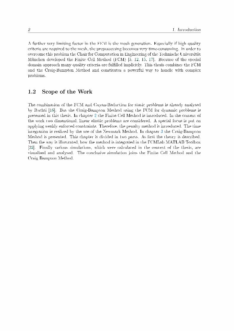
A further very limiting factor in the FEM is the mesh generation. Especially if high qualitycriteria are required to the mesh, the prepossessing becomes very time-consuming. In order toovercome this problem the Chair for Computation in Engineering of the Technische UniversitätMünchen developed the Finite Cell Method (FCM) [5, 12, 15, 17]. Because of the specialdomain approach many quality criteria are fullled implicitly. This thesis combines the FCMand the Craig-Bampton Method and constitutes a powerful way to handle with complexproblems.
1.2 Scope of the Work
The combination of the FCM and Guyan-Reduction for static problems is already analysedby Ruchti [16]. But the Craig-Bampton Method using the FCM for dynamic problems ispresented in this thesis. In chapter 2 the Finite Cell Method is introduced. In the context ofthe work two dimensional, linear elastic problems are considered. A special focus is put onapplying weakly enforced constraints. Therefore, the penalty method is introduced. The timeintegration is realized by the use of the Newmark Method. In chapter 3 the Craig-BamptonMethod is presented. This chapter is divided in two parts. At rst the theory is described.Then the way is illustrated, how the method is integrated in the FCMLab MATLAB Toolbox[22]. Finally various simulations, which were calculated in the context of the thesis, arevisualised and analysed. The conclusive simulation joins the Finite Cell Method and theCraig-Bampton Method.
3
Chapter 2
The Finite Cell Method for Structural
Dynamics
A very common numerical method in order to solve problems in structural mechanics is theFinite Element Method (FEM) [2, 10, 18]. One of the limiting factors of the FEM is themesh generation. Especially for non-trivial geometries in combination with high quality meshcriteria the mesh generation may becomes very complex and time-consuming. In order to solvethis problem the Finite Cell Method (FCM) was developed by the Chair for Computation inEngineering (CiE) [5, 12, 15, 17]. The concept of the FCM is presented in this chapter. Basedon the governing equations of linear elastodynamics, introduced in section 2.1, the conceptsof high order shape functions, section 2.2, and the embedded domain approach, section 2.3are described. Because of the special domain approach a adaptive integration scheme isintroduced in section 2.4. Furthermore, weakly enforced boundary and interface constraintsare presented in section 2.5. The resultant time-dependent equation can be solved by theNewmark method, which is introduced in section 2.6.
2.1 Weak Formulation of the Linear Elastodynamic Equation
The standard problem in structural dynamics is a elastic continuum with the domain Ω andits boundary δΩ. There are two dierent types of boundaries, Dirichlet ΓD and Neumann ΓNboundaries, which have to satisfy the following conditions: ΓD∪ΓN = δΩ and ΓD∩ΓN = 0.
According to Wall [19] the following initial-boundary value problem (IBVP) describes theproperties for the linear elastodynamic problem. The formulation of the IBVP is called strongformulation.
Field equations:
Balance equation (BE): ∇ · σ + b = ρu in Ω× [t0, tend] (2.1a)
Constitutive equation (CE): σ = C : ε (2.1b)

4 2. The Finite Cell Method for Structural Dynamics
Kinematic equation (KE): ε = 12(∇u+ (∇u)T ) (2.1c)
Velocities: u = ddtu (2.1d)
Accelerations: u = ddt u = d2
dt2u (2.1e)
where σ is the stress tensor, ε the strain tensor, C the forth order elasticity tensor, b thebody force vector, ρ the density and u the displacement vector.
Boundary conditions (BC):
Dirichlet BC (DBC): u = u on ΓD × [t0, tend] (2.1f)
Neumann BC (NBC): σ · n = t on ΓN × [t0, tend] (2.1g)
where u is the prescribed boundary displacement vector, n the unit normal vector and t thegiven boundary traction vector.
Initial conditions (IC):
u(x, t0) = u0 in Ω (2.1h)
u(x, t0) = ˆu0 in Ω (2.1i)
where u0 is the given initial displacement and ˆu0 the given initial velocity.
In real life problems, it's usually not possible to nd an analytical solution of the strongformulation of the IBVP. Hence, approximation methods are needed to obtain a solution. Avery suitable method for structural problems is the nite element method, which is based onthe weak formulation of the IBVP. Therefore, the balance equation (2.1a) is integrated overthe domain Ω and weighted by a test function v ∈ V [10, 19]:
∫Ω
(∇ · σ + b− ρu) · v dΩ v ∈ V, (2.2)
with V = v | v ∈ H1, v(xD) = 0 : xD ∈ ΩD, (2.3)
U = u | u ∈ H1, u(xD) = u : xD ∈ ΩD (2.4)
and H1 are the functions of the rst order Sobolev space.
This equation is also called equation of virtual work and its trail function u ∈ U , whichsatises the equation for any test function v ∈ V, is called weak solution. When using theinnite-dimensional Sobolev space, the weak solution is exact. For further considerations thedivergence theorem and the approach for the test function at the Dirichlet boundary is appliedon the equation of virtual work (2.2). This yields in the following weak form of the equationof motion [6]:
2.1. Weak Formulation of the Linear Elastodynamic Equation 5
D(u,v) + B(u,v) = F(v), (2.5)
D(u,v) =
∫Ωρu · v dΩ, (2.6)
B(u,v) =
∫Ωε(v) : C : ε(u) dΩ, (2.7)
F(v) =
∫Ωb · v dΩ +
∫ΓN
t · v dΓ. (2.8)
The Finite Element Method only uses a n-dimensional subspace of the Sobolev space, whichyields an approximate solution uh. According to the Bubnov-Galerkin approach, the trailfunctions uh ∈ Uh and the test functions vh ∈ Vh have the same function space, which isspanned by the shape functions N1,N2, . . . ,Nn. The approximate solution uh is the linearcombination of the shape functions with the associated degrees of freedom u [22]:
uh =n∑i=1
Niui, (2.9)
vh =n∑i=1
Nivi. (2.10)
When inserting these equations into the weak form of the equation of motion (2.5), a systemof linear equations can be obtained, which is called the semi-discrete equation of motion
Mu(t) + Ku(t) = F(t). (2.11)
The mass matrix M, stiness matrix K and the load vector F can be calculated from theirelemental matrices me, ke and fe. Therefore, the domain Ω is divided into multiple elementsΩe and the boundary Γ is divided into multiple boundary segments Γn:
me =
∫Ωe
NTρN dΩ, (2.12)
ke =
∫Ωe
BTCB dΩ, (2.13)
fe =
∫Ωe
NT · b dΩ +
∫Γn
NT · t dΓ, (2.14)
where N is the shape function vector, B is the strain-displacement matrix and C is theelasticity matrix.
6 2. The Finite Cell Method for Structural Dynamics
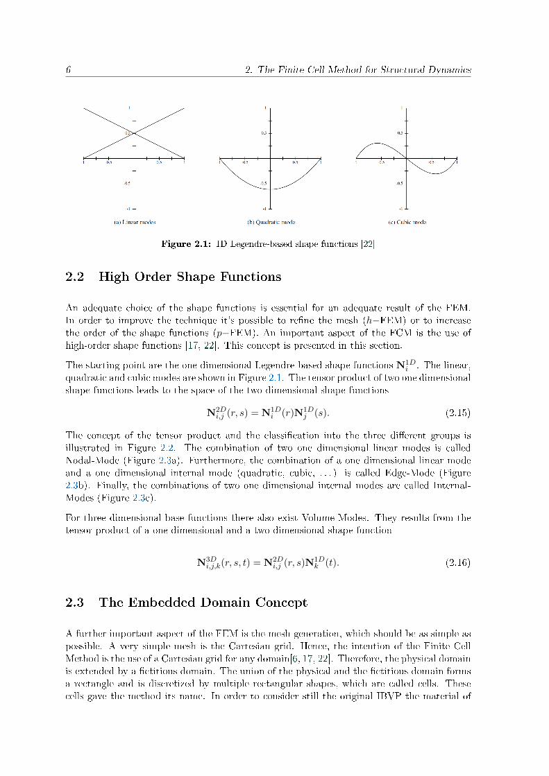
Figure 2.1: 1D Legendre-based shape functions [22]
2.2 High Order Shape Functions
An adequate choice of the shape functions is essential for an adequate result of the FEM.In order to improve the technique it's possible to rene the mesh (h−FEM) or to increasethe order of the shape functions (p−FEM). An important aspect of the FCM is the use ofhigh-order shape functions [17, 22]. This concept is presented in this section.
The starting point are the one dimensional Legendre-based shape functions N1Di . The linear,
quadratic and cubic modes are shown in Figure 2.1. The tensor product of two one dimensionalshape functions leads to the space of the two dimensional shape functions
N2Di,j (r, s) = N1D
i (r)N1Dj (s). (2.15)
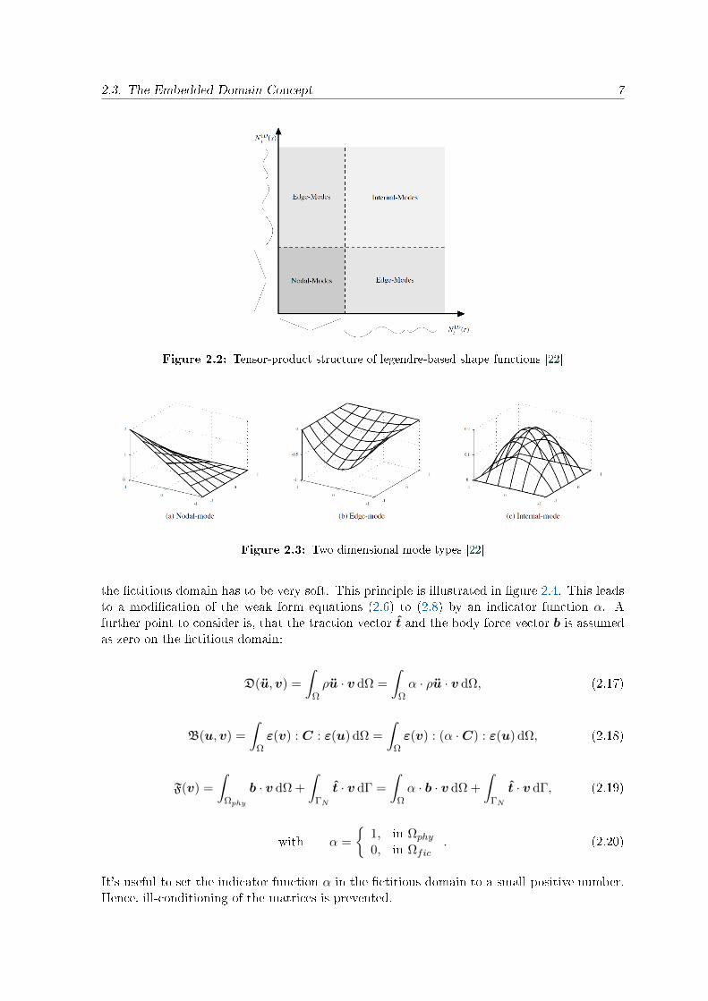
The concept of the tensor product and the classication into the three dierent groups isillustrated in Figure 2.2. The combination of two one dimensional linear modes is calledNodal-Mode (Figure 2.3a). Furthermore, the combination of a one dimensional linear modeand a one dimensional internal mode (quadratic, cubic, . . . ) is called Edge-Mode (Figure2.3b). Finally, the combinations of two one dimensional internal modes are called Internal-Modes (Figure 2.3c).
For three dimensional base functions there also exist Volume-Modes. They results from thetensor product of a one dimensional and a two dimensional shape function
N3Di,j,k(r, s, t) = N2D
i,j (r, s)N1Dk (t). (2.16)
2.3 The Embedded Domain Concept
A further important aspect of the FEM is the mesh generation, which should be as simple aspossible. A very simple mesh is the Cartesian grid. Hence, the intention of the Finite CellMethod is the use of a Cartesian grid for any domain[6, 17, 22]. Therefore, the physical domainis extended by a ctitious domain. The union of the physical and the ctitious domain formsa rectangle and is discretized by multiple rectangular shapes, which are called cells. Thesecells gave the method its name. In order to consider still the original IBVP the material of
2.3. The Embedded Domain Concept 7
Figure 2.2: Tensor-product structure of legendre-based shape functions [22]
Figure 2.3: Two dimensional mode types [22]
the ctitious domain has to be very soft. This principle is illustrated in gure 2.4. This leadsto a modication of the weak form equations (2.6) to (2.8) by an indicator function α. Afurther point to consider is, that the traction vector t and the body force vector b is assumedas zero on the ctitious domain:
D(u,v) =
∫Ωρu · v dΩ =
∫Ωα · ρu · v dΩ, (2.17)
B(u,v) =
∫Ωε(v) : C : ε(u) dΩ =
∫Ωε(v) : (α ·C) : ε(u) dΩ, (2.18)
F(v) =
∫Ωphy
b · v dΩ +
∫ΓN
t · v dΓ =
∫Ωα · b · v dΩ +
∫ΓN
t · v dΓ, (2.19)
with α =
1, in Ωphy
0, in Ωfic. (2.20)
It's useful to set the indicator function α in the ctitious domain to a small positive number.Hence, ill-conditioning of the matrices is prevented.

8 2. The Finite Cell Method for Structural Dynamics
Figure 2.4: The nite cell idea [17] [22]
Figure 2.5: Integration via space-trees [17] [22]
2.4 Adaptive Integration
In contrast to the integration in cells, which belong totally either to the physical or the c-titious domain, a suitable integration in cells cut by the boundary is not trivial. A precisedistinction of the physical and ctitious part of a cell is necessary. Hence, a separate integra-tion mesh is introduced [17, 22]. Except for the cells cut by the boundary, this integrationmesh is equal to the Cartesian mesh introduced in section 2.3. The cells cut by the bound-ary are rened by using a quad-structure as illustrated in gure 2.5. For 3D problems anoctree-structure is used.
Because of the non-conforming mesh and the boundary geometry, a further challenge is theintegration over the boundary. This integration is necessary for applying Neumann boundaryconditions (see equation (2.19)), weakly enforced Dirichlet boundary conditions and weaklyenforced interface constraints, which are described in the next section 2.5. Similar to theintegration mesh a surface integration mesh is needed here.
2.5. Weakly Enforced Boundary and Interface Constraints 9
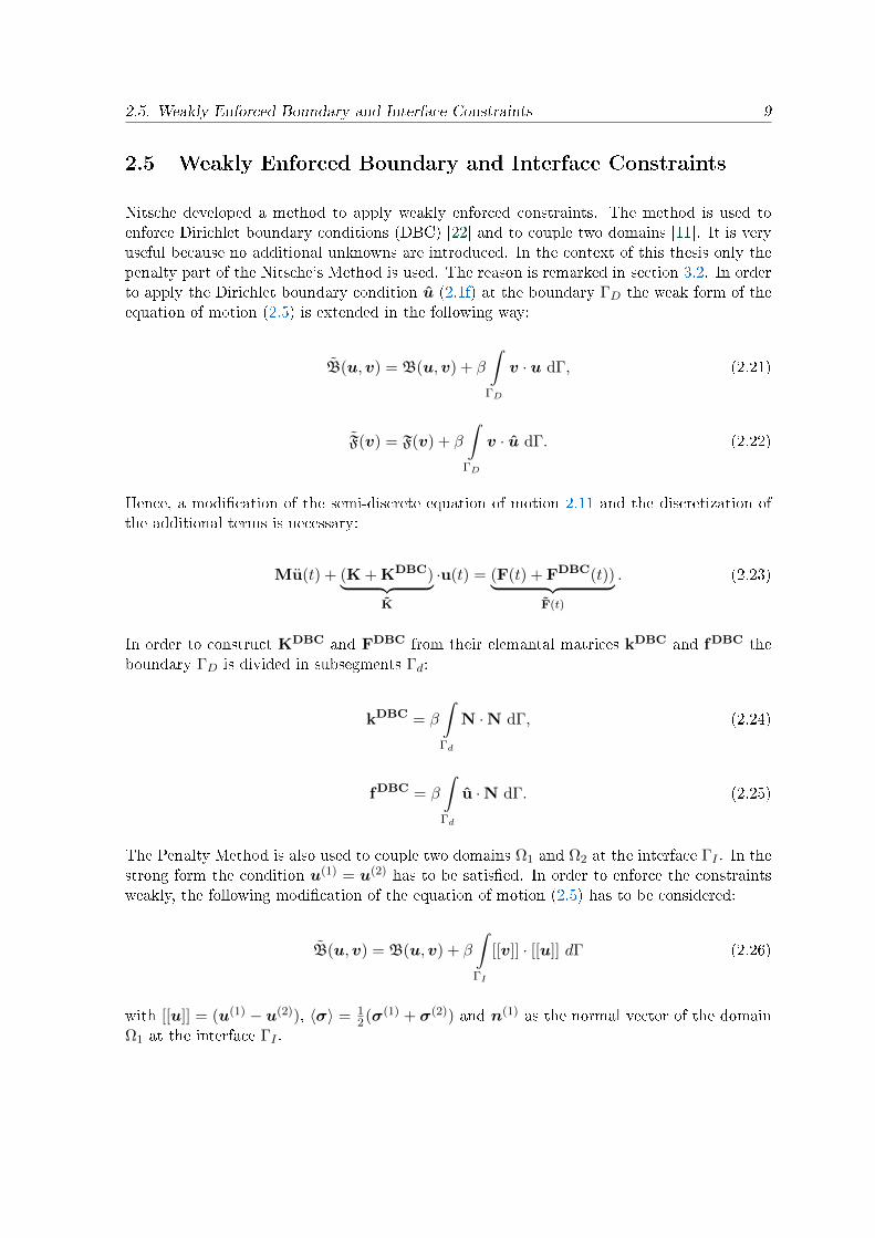
2.5 Weakly Enforced Boundary and Interface Constraints
Nitsche developed a method to apply weakly enforced constraints. The method is used toenforce Dirichlet boundary conditions (DBC) [22] and to couple two domains [11]. It is veryuseful because no additional unknowns are introduced. In the context of this thesis only thepenalty part of the Nitsche's Method is used. The reason is remarked in section 3.2. In orderto apply the Dirichlet boundary condition u (2.1f) at the boundary ΓD the weak form of theequation of motion (2.5) is extended in the following way:
B(u,v) = B(u,v) + β
∫ΓD
v · u dΓ, (2.21)
F(v) = F(v) + β
∫ΓD
v · u dΓ. (2.22)
Hence, a modication of the semi-discrete equation of motion 2.11 and the discretization ofthe additional terms is necessary:
Mu(t) + (K + KDBC)︸ ︷︷ ︸K
·u(t) = (F(t) + FDBC(t))︸ ︷︷ ︸F(t)
. (2.23)
In order to construct KDBC and FDBC from their elemantal matrices kDBC and fDBC theboundary ΓD is divided in subsegments Γd:
kDBC = β
∫Γd
N ·N dΓ, (2.24)
fDBC = β
∫Γd
u ·N dΓ. (2.25)
The Penalty Method is also used to couple two domains Ω1 and Ω2 at the interface ΓI . In thestrong form the condition u(1) = u(2) has to be satised. In order to enforce the constraintsweakly, the following modication of the equation of motion (2.5) has to be considered:
B(u,v) = B(u,v) + β
∫ΓI
[[v]] · [[u]] dΓ (2.26)
with [[u]] = (u(1) − u(2)), 〈σ〉 = 12(σ(1) + σ(2)) and n(1) as the normal vector of the domain
Ω1 at the interface ΓI .
10 2. The Finite Cell Method for Structural Dynamics
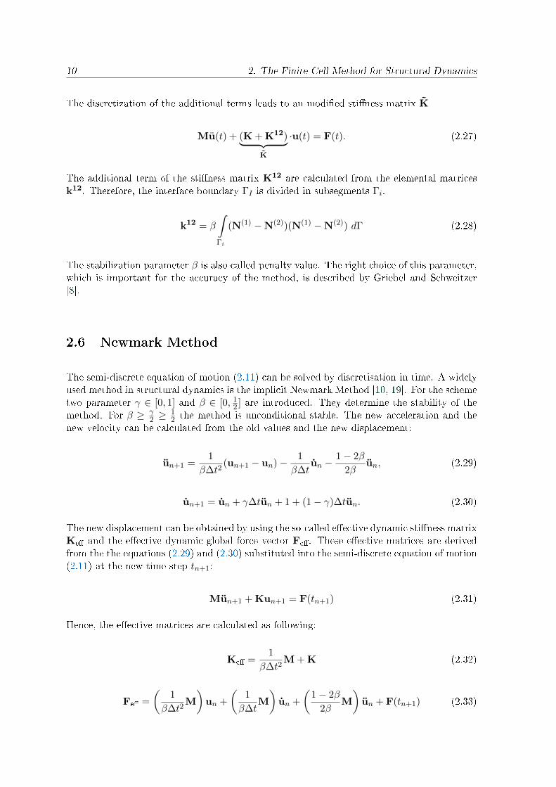
The discretization of the additional terms leads to an modied stiness matrix K
Mu(t) + (K + K12)︸ ︷︷ ︸K
·u(t) = F(t). (2.27)
The additional term of the stiness matrix K12 are calculated from the elemental matricesk12. Therefore, the interface boundary ΓI is divided in subsegments Γi.
k12 = β
∫Γi
(N(1) −N(2))(N(1) −N(2)) dΓ (2.28)
The stabilization parameter β is also called penalty value. The right choice of this parameter,which is important for the accuracy of the method, is described by Griebel and Schweitzer[8].
2.6 Newmark Method
The semi-discrete equation of motion (2.11) can be solved by discretisation in time. A widelyused method in structural dynamics is the implicit Newmark Method [10, 19]. For the schemetwo parameter γ ∈ [0, 1] and β ∈ [0, 1
2 ] are introduced. They determine the stability of themethod. For β ≥ γ
2 ≥12 the method is unconditional stable. The new acceleration and the
new velocity can be calculated from the old values and the new displacement:
un+1 =1
β∆t2(un+1 − un)− 1
β∆tun −
1− 2β
2βun, (2.29)
un+1 = un + γ∆tun + 1 + (1− γ)∆tun. (2.30)
The new displacement can be obtained by using the so-called eective dynamic stiness matrixKe and the eective dynamic global force vector Fe. These eective matrices are derivedfrom the the equations (2.29) and (2.30) substituted into the semi-discrete equation of motion(2.11) at the new time step tn+1:
Mun+1 + Kun+1 = F(tn+1) (2.31)
Hence, the eective matrices are calculated as following:
Ke =1
β∆t2M + K (2.32)
Fe =
(1
β∆t2M
)un +
(1
β∆tM
)un +
(1− 2β
2βM
)un + F(tn+1) (2.33)

2.6. Newmark Method 11
Keun+1 = Fe (2.34)
This equation can be solved according to the usual practice.

12 2. The Finite Cell Method for Structural Dynamics
13
Chapter 3
Generation of Superelements using the
Finite Cell Method
For large domains with increasing renement and increasing order of the shape functions thenumber of degrees of freedom becomes very large. Solving these complex systems is verytime-consuming. In order to achieve a shorter runtime, parts of a system can be treated assuper elements with a reduced number of degrees of freedom (DOFs). A further advantagerelated to the runtime is, that a super element can be calculated in advance and stored inan Super Element Library. During the runtime the super element can be loaded from thisSuper Element Library.
In order to decrease the number of degrees of freedom of a super element dierent reductionmethods have been developed [4]. A static reduction method is the Guyan-Irons reduction[9]. For dynamic problems especially in the high-frequency range this method isn't suitable,because a proper reduction of the mass matrix has to be considered. In order to get accurateresults for dynamic problems component modes have to be considered. In this thesis the Craig- Bampton Method (section 3.1) , which uses xed-interface normal modes in combinationwith interface constraint modes, is presented [1, 4, 21]. In the second part of this chapter(section 3.2) it is illustrated how this method is integrated in the FCMLab MATLAB Toolbox[22], which was developed by the Chair for Computation in Engineering.
3.1 Craig-Bampton Method
The degrees of freedom are divided into a boundary part b as master DOFs and an internalpart i as slave DOFs. Hence, the semi-discret equation of motion 2.11 gets the followingpartitioned form:
[Mii Mib
Mbi Mbb
] [uiub
]+
[Kii Kib
Kbi Kbb
] [uiub
]=
[Fi
Fb
]. (3.1)
The aim of the Craig-Bampton Method is the reduction of the internal degrees of freedom byconsidering a dened number of internal modes.
14 3. Generation of Superelements using the Finite Cell Method
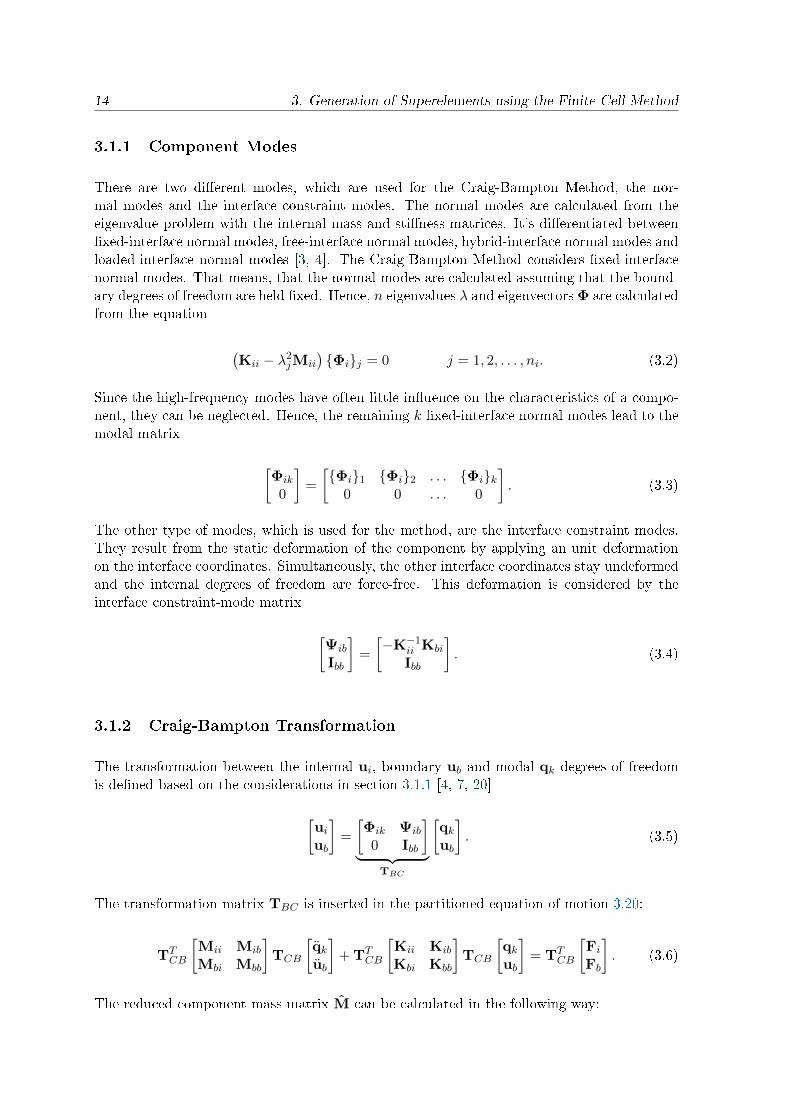
3.1.1 Component Modes
There are two dierent modes, which are used for the Craig-Bampton Method, the nor-mal modes and the interface constraint modes. The normal modes are calculated from theeigenvalue problem with the internal mass and stiness matrices. It's dierentiated betweenxed-interface normal modes, free-interface normal modes, hybrid-interface normal modes andloaded-interface normal modes [3, 4]. The Craig-Bampton Method considers xed-interfacenormal modes. That means, that the normal modes are calculated assuming that the bound-ary degrees of freedom are held xed. Hence, n eigenvalues λ and eigenvectors Φ are calculatedfrom the equation
(Kii − λ2
jMii
)Φij = 0 j = 1, 2, . . . , ni. (3.2)
Since the high-frequency modes have often little inuence on the characteristics of a compo-nent, they can be neglected. Hence, the remaining k xed-interface normal modes lead to themodal matrix
[Φik
0
]=
[Φi1 Φi2 . . . Φik
0 0 . . . 0
]. (3.3)
The other type of modes, which is used for the method, are the interface constraint modes.They result from the static deformation of the component by applying an unit deformationon the interface coordinates. Simultaneously, the other interface coordinates stay undeformedand the internal degrees of freedom are force-free. This deformation is considered by theinterface constraint-mode matrix
[Ψib
Ibb
]=
[−K−1
ii Kbi
Ibb
]. (3.4)
3.1.2 Craig-Bampton Transformation
The transformation between the internal ui, boundary ub and modal qk degrees of freedomis dened based on the considerations in section 3.1.1 [4, 7, 20]
[uiub
]=
[Φik Ψib
0 Ibb
]︸ ︷︷ ︸
TBC
[qkub
]. (3.5)
The transformation matrix TBC is inserted in the partitioned equation of motion 3.20:
TTCB
[Mii Mib
Mbi Mbb
]TCB
[qkub
]+ TT
CB
[Kii Kib
Kbi Kbb
]TCB
[qkub
]= TT
CB
[Fi
Fb
]. (3.6)
The reduced component mass matrix M can be calculated in the following way:
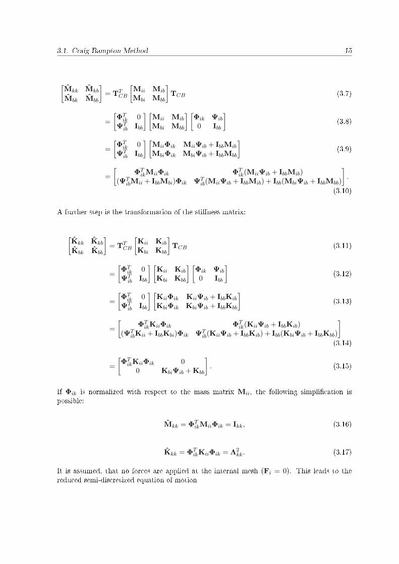
3.1. Craig-Bampton Method 15
[Mkk Mkb
Mbk Mbb
]= TT
CB
[Mii Mib
Mbi Mbb
]TCB (3.7)
=
[ΦTik 0
ΨTib Ibb
] [Mii Mib
Mbi Mbb
] [Φik Ψib
0 Ibb
](3.8)
=
[ΦTik 0
ΨTib Ibb
] [MiiΦik MiiΨib + IbbMib
MbiΦik MbiΨib + IbbMbb
](3.9)
=
[ΦTikMiiΦik ΦT
ik(MiiΨib + IbbMib)(ΨT
ibMii + IbbMbi)Φik ΨTib(MiiΨib + IbbMib) + Ibb(MbiΨib + IbbMbb)
].
(3.10)
A further step is the transformation of the stiness matrix:
[Kkk Kkb
Kbk Kbb
]= TT
CB
[Kii Kib
Kbi Kbb
]TCB (3.11)
=
[ΦTik 0
ΨTib Ibb
] [Kii Kib
Kbi Kbb
] [Φik Ψib
0 Ibb
](3.12)
=
[ΦTik 0
ΨTib Ibb
] [KiiΦik KiiΨib + IbbKib
KbiΦik KbiΨib + IbbKbb
](3.13)
=
[ΦTikKiiΦik ΦT
ik(KiiΨib + IbbKib)(ΨT
ibKii + IbbKbi)Φik ΨTib(KiiΨib + IbbKib) + Ibb(KbiΨib + IbbKbb)
](3.14)
=
[ΦTikKiiΦik 0
0 KbiΨib + Kbb
]. (3.15)
If Φik is normalized with respect to the mass matrix Mii, the following simplication ispossible:
Mkk = ΦTikMiiΦik = Ikk, (3.16)
Kkk = ΦTikKiiΦik = Λ2
kk. (3.17)
It is assumed, that no forces are applied at the internal mesh (Fi = 0). This leads to thereduced semi-discretized equation of motion
16 3. Generation of Superelements using the Finite Cell Method
[Ikk Mkb
Mbk Mbb
] [qkub
]+
[Λ2kk 0
0 Kbb
] [qkub
]=
[0Fb
], (3.18)
which can be solved in time by the Newmark method (see section 2.6).
3.1.3 Substructuring and Super Elements
Using the Craig-Bampton Method the boundary coordinates are kept as independent gener-alized coordinates. Thus, it is possible to couple the super element at this boundary to othercomponents. Hence, the reduced model based on the xed-interface modes in combinationwith the interface constraint modes is called super element [4].
It's also possible to connect two super elements. Thus, complex structures with super elementscan be created. Every element can have a dierent structure and a dierent number of keptmodes. The technique of dividing a complex structure into multiple super elements is calledsubstructuring. [2, 13]
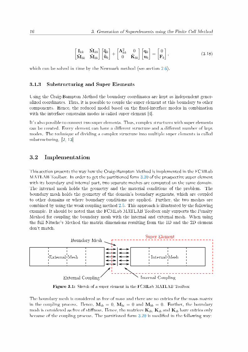
3.2 Implementation
This section presents the way how the Craig-Bampton Method is implemented in the FCMLabMATLAB Toolbox. In order to get the partitioned form 3.20 of the prospective super elementwith its boundary and internal part, two separate meshes are computed on the same domain.The internal mesh holds the geometry and the material conditions of the problem. Theboundary mesh holds the geometry of the domain's boundary segments, which are coupledto other domains or where boundary conditions are applied. Further, the two meshes arecombined by using the weak coupling method 2.5. This approach is illustrated by the followingexample. It should be noted that the FCMLab MATLAB Toolbox only supports the PenaltyMethod for coupling the boundary mesh with the internal and external mesh. When usingthe full Nitsche's Method the matrix dimensions resulting from the 1D and the 2D elementdon't match.
Super Element
External Mesh Internal Mesh
Boundary Mesh
External Coupling Internal Coupling
Figure 3.1: Sketch of a super element in the FCMLab MATLAB Toolbox
The boundary mesh is considered as free of mass and there are no entries for the mass matrixin the coupling process. Hence, Mib = 0, Mbi = 0 and Mbb = 0. Further, the boundarymesh is considered as free of stiness. Hence, the matrices Kib, Kib and Kib have entries onlybecause of the coupling process. The partitioned form 3.20 is modied in the following way:
3.2. Implementation 17
[Mii 0
0 0
] [uiub
]+
[Kii Kib
Kbi Kbb
] [uiub
]=
[0Fb
](3.19)
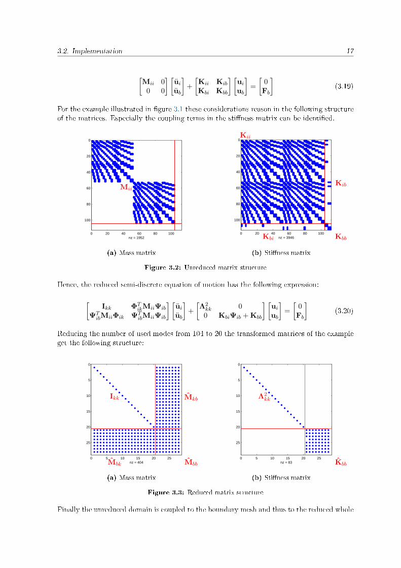
For the example illustrated in gure 3.1 these considerations reason in the following structureof the matrices. Especially the coupling terms in the stiness matrix can be identied.
0 20 40 60 80 100
0
20
40
60
80
100
nz = 1952
Mii
(a) Mass matrix
0 20 40 60 80 100
0
20
40
60
80
100
nz = 3946
Kii
Kbb
Kib
Kbi
(b) Stiness matrix
Figure 3.2: Unreduced matrix structure
Hence, the reduced semi-discrete equation of motion has the following expression:
[Ikk ΦT
ikMiiΨib
ΨTibMiiΦik ΨT
ibMiiΨib
] [uiub
]+
[Λ2kk 00 KbiΨib + Kbb
] [uiub
]=
[0Fb
](3.20)
Reducing the number of used modes from 104 to 20 the transformed matrices of the exampleget the following structure:
0 5 10 15 20 25
0
5
10
15
20
25
nz = 404
Ikk
Mbb
Mkb
Mbk
(a) Mass matrix
0 5 10 15 20 25
0
5
10
15
20
25
nz = 83
Λ2kk
Kbb
(b) Stiness matrix
Figure 3.3: Reduced matrix structure
Finally the unreduced domain is coupled to the boundary mesh and thus to the reduced whole
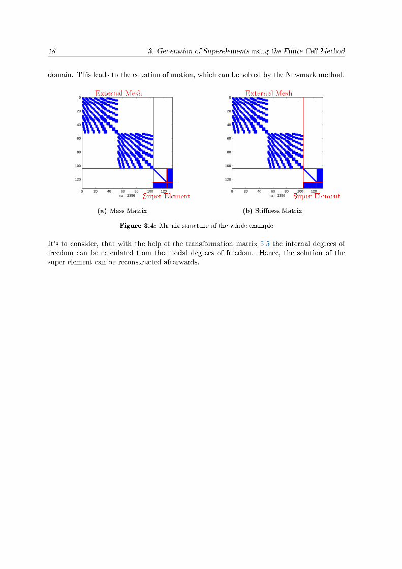
18 3. Generation of Superelements using the Finite Cell Method
domain. This leads to the equation of motion, which can be solved by the Newmark method.
0 20 40 60 80 100 120
0
20
40
60
80
100
120
nz = 2356
External Mesh
Super Element
(a) Mass Matrix
0 20 40 60 80 100 120
0
20
40
60
80
100
120
nz = 2356
External Mesh
Super Element
(b) Stiness Matrix
Figure 3.4: Matrix structure of the whole example
It's to consider, that with the help of the transformation matrix 3.5 the internal degrees offreedom can be calculated from the modal degrees of freedom. Hence, the solution of thesuper element can be reconstructed afterwards.
19
Chapter 4
Numerical Examples
4.1 Periodic Excitation of a 2D Bar
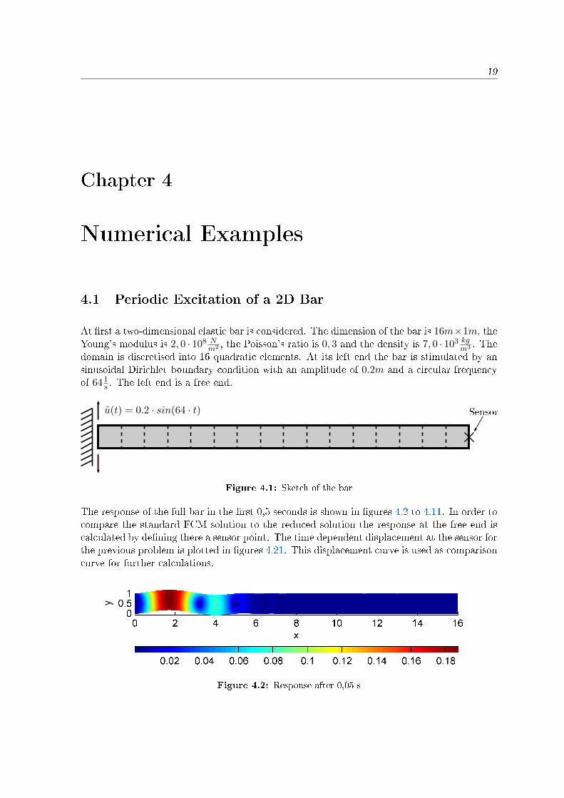
At rst a two-dimensional elastic bar is considered. The dimension of the bar is 16m×1m, theYoung's modulus is 2, 0 · 108 N
m2 , the Poisson's ratio is 0, 3 and the density is 7, 0 · 103 kgm3 . The
domain is discretised into 16 quadratic elements. At its left end the bar is stimulated by ansinusoidal Dirichlet boundary condition with an amplitude of 0.2m and a circular frequencyof 641
s . The left end is a free end.
u(t) = 0.2 · sin(64 · t) Sensor
Figure 4.1: Sketch of the bar
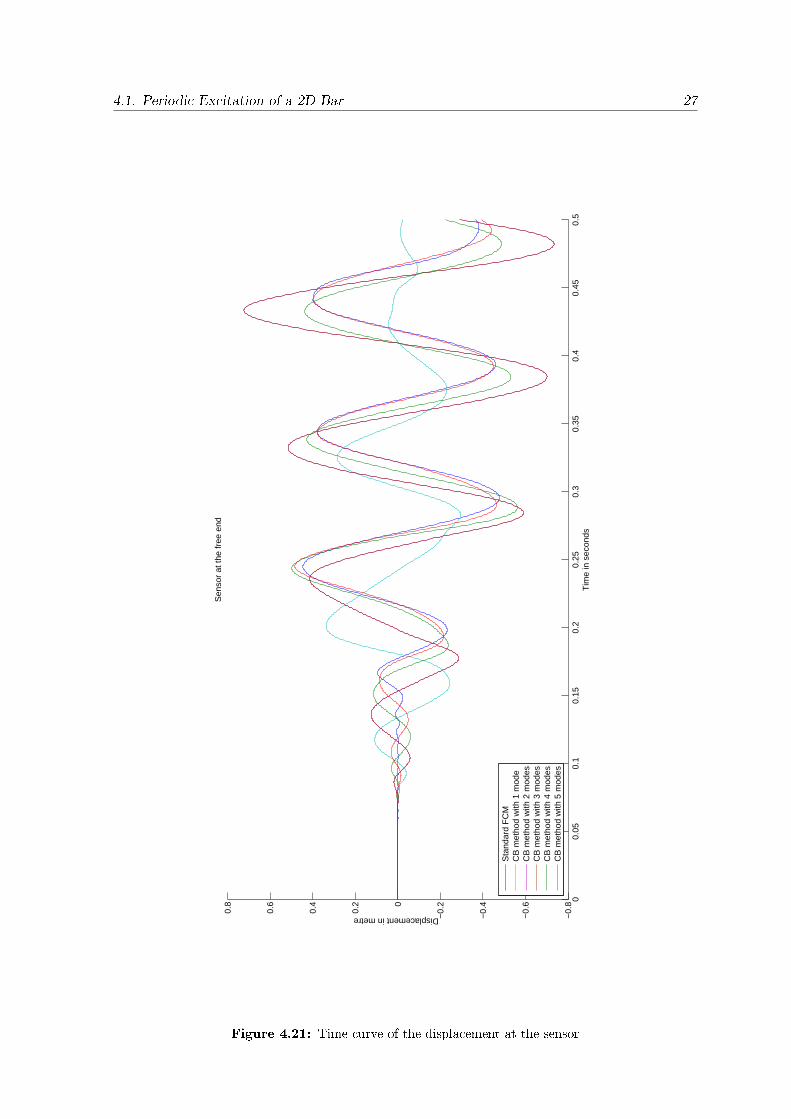
The response of the full bar in the rst 0,5 seconds is shown in gures 4.2 to 4.11. In order tocompare the standard FCM solution to the reduced solution the response at the free end iscalculated by dening there a sensor point. The time dependent displacement at the sensor forthe previous problem is plotted in gures 4.21. This displacement curve is used as comparisoncurve for further calculations.
Figure 4.2: Response after 0,05 s

20 4. Numerical Examples
Figure 4.3: Response after 0,1 s
Figure 4.4: Response after 0,15 s
Figure 4.5: Response after 0,20 s
Figure 4.6: Response after 0,25 s
Figure 4.7: Response after 0,3 s

4.1. Periodic Excitation of a 2D Bar 21
Figure 4.8: Response after 0,35 s
Figure 4.9: Response after 0,4 s
Figure 4.10: Response after 0,45 s
Figure 4.11: Response after 0,5 s

22 4. Numerical Examples
00.
050.
10.
150.
20.
250.
30.
350.
40.
450.
5−
0.5
−0.
4
−0.
3
−0.
2
−0.
10
0.1
0.2
0.3
0.4
0.5
Sen
sor
at th
e fr
ee e
nd
Tim
e in
sec
onds
Displacement in metre
Figure 4.12: Response over time at the right free end
4.1. Periodic Excitation of a 2D Bar 23
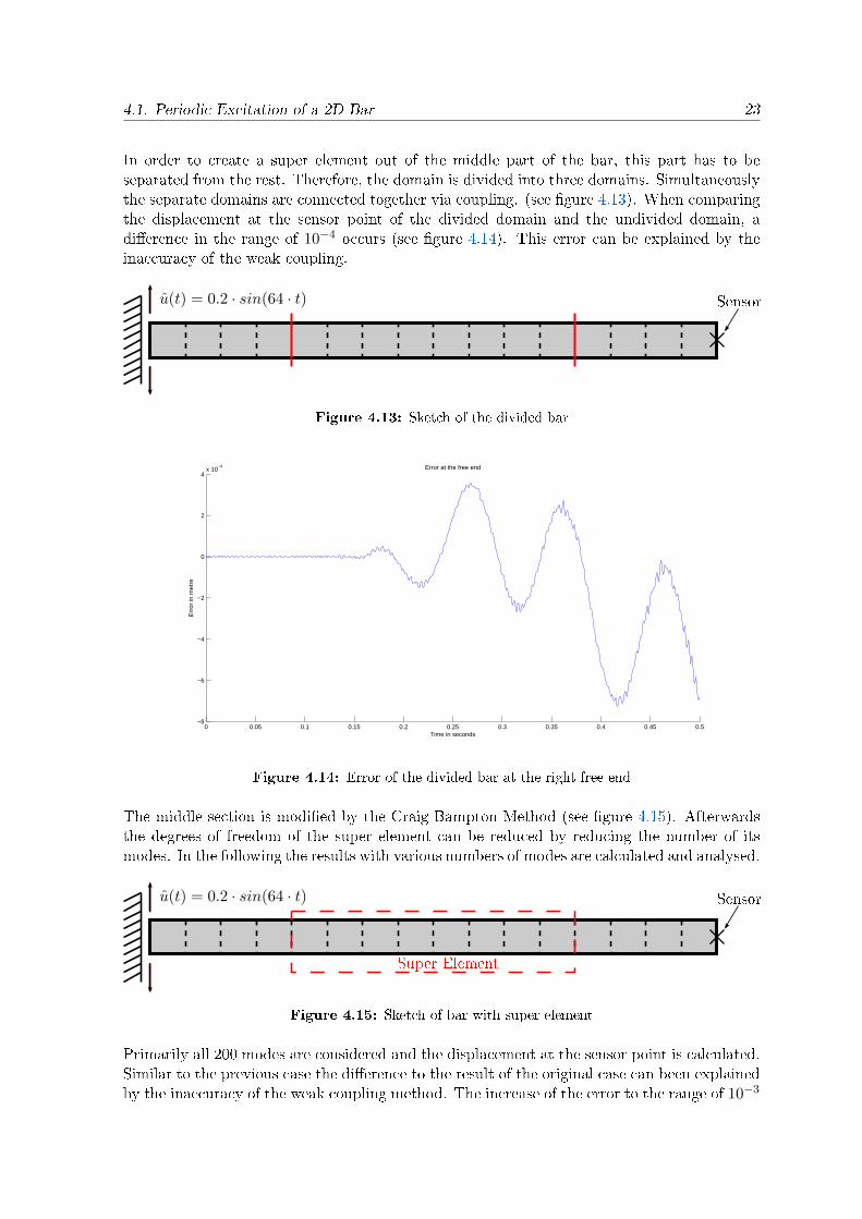
In order to create a super element out of the middle part of the bar, this part has to beseparated from the rest. Therefore, the domain is divided into three domains. Simultaneouslythe separate domains are connected together via coupling. (see gure 4.13). When comparingthe displacement at the sensor point of the divided domain and the undivided domain, adierence in the range of 10−4 occurs (see gure 4.14). This error can be explained by theinaccuracy of the weak coupling.
u(t) = 0.2 · sin(64 · t) Sensor
Figure 4.13: Sketch of the divided bar
0 0.05 0.1 0.15 0.2 0.25 0.3 0.35 0.4 0.45 0.5−8
−6
−4
−2
0
2
4x 10
−4 Error at the free end
Time in seconds
Err
or in
met
re
Figure 4.14: Error of the divided bar at the right free end
The middle section is modied by the Craig-Bampton Method (see gure 4.15). Afterwardsthe degrees of freedom of the super element can be reduced by reducing the number of itsmodes. In the following the results with various numbers of modes are calculated and analysed.
u(t) = 0.2 · sin(64 · t) Sensor
Super Element
Figure 4.15: Sketch of bar with super element
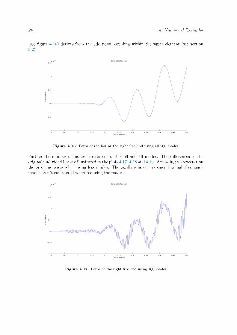
Primarily all 200 modes are considered and the displacement at the sensor point is calculated.Similar to the previous case the dierence to the result of the original case can been explainedby the inaccuracy of the weak coupling method. The increase of the error to the range of 10−3
24 4. Numerical Examples
(see gure 4.16) derives from the additional coupling within the super element (see section3.2).
0 0.05 0.1 0.15 0.2 0.25 0.3 0.35 0.4 0.45 0.5−1
−0.5
0
0.5
1
1.5x 10
−3 Error at the free end
Time in seconds
Err
or in
met
re
Figure 4.16: Error of the bar at the right free end using all 200 modes
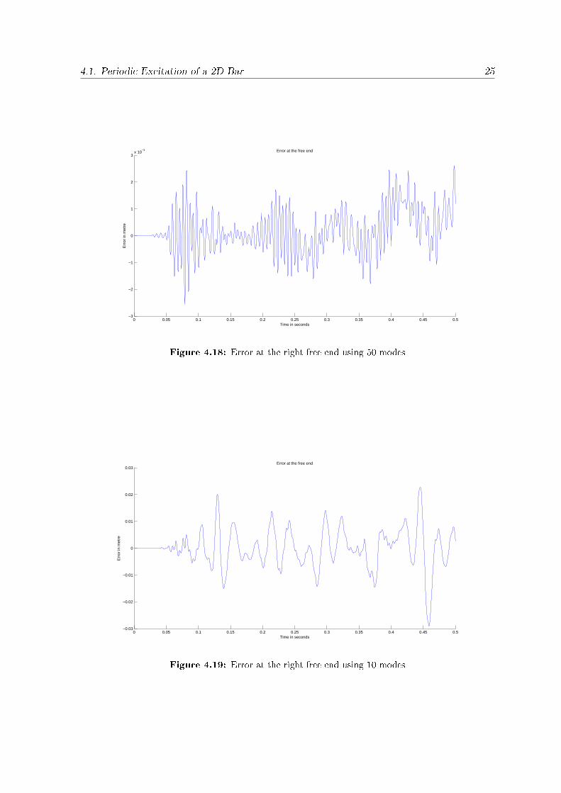
Further the number of modes is reduced to 100, 50 and 10 modes. The dierences to theoriginal undivided bar are illustrated in the plots 4.17, 4.18 and 4.19. According to expectationthe error increases when using less modes. The oscillations occurs since the high frequencymodes aren't considered when reducing the modes.
0 0.05 0.1 0.15 0.2 0.25 0.3 0.35 0.4 0.45 0.5−1
−0.5
0
0.5
1
1.5
2x 10
−3 Error at the free end
Time in seconds
Err
or in
met
re
Figure 4.17: Error at the right free end using 100 modes
4.1. Periodic Excitation of a 2D Bar 25
0 0.05 0.1 0.15 0.2 0.25 0.3 0.35 0.4 0.45 0.5−3
−2
−1
0
1
2
3x 10
−3 Error at the free end
Time in seconds
Err
or in
met
re
Figure 4.18: Error at the right free end using 50 modes
0 0.05 0.1 0.15 0.2 0.25 0.3 0.35 0.4 0.45 0.5−0.03
−0.02
−0.01
0
0.01
0.02
0.03Error at the free end
Time in seconds
Err
or in
met
re
Figure 4.19: Error at the right free end using 10 modes
26 4. Numerical Examples
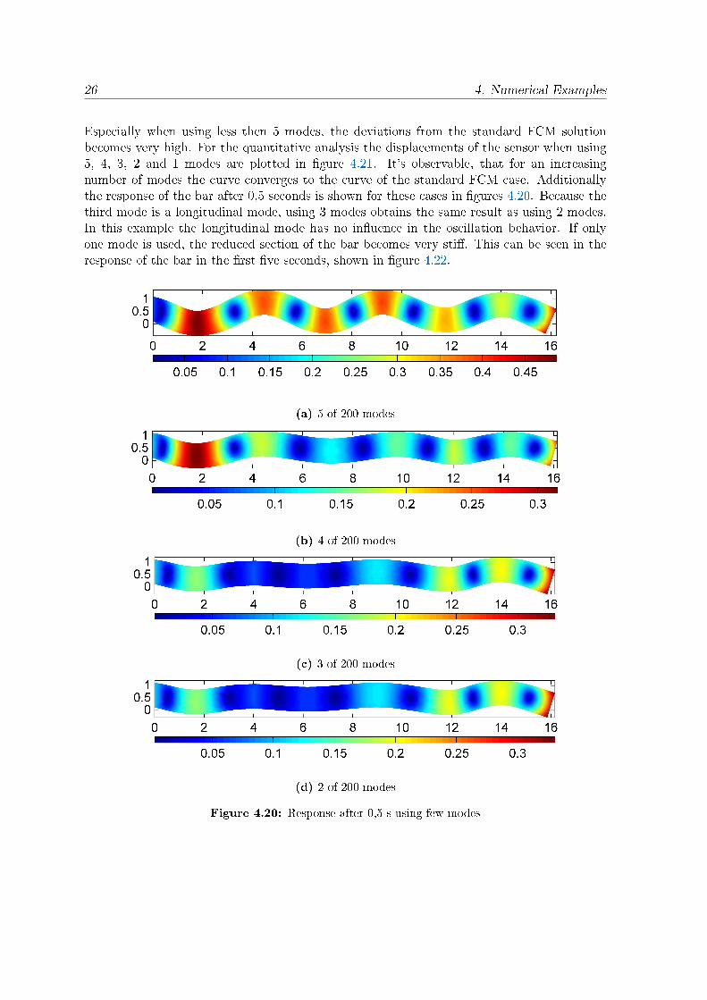
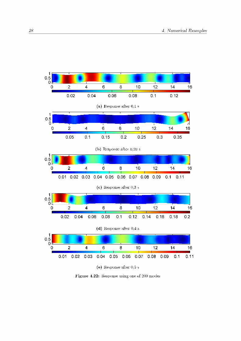
Especially when using less then 5 modes, the deviations from the standard FCM solutionbecomes very high. For the quantitative analysis the displacements of the sensor when using5, 4, 3, 2 and 1 modes are plotted in gure 4.21. It's observable, that for an increasingnumber of modes the curve converges to the curve of the standard FCM case. Additionallythe response of the bar after 0,5 seconds is shown for these cases in gures 4.20. Because thethird mode is a longitudinal mode, using 3 modes obtains the same result as using 2 modes.In this example the longitudinal mode has no inuence in the oscillation behavior. If onlyone mode is used, the reduced section of the bar becomes very sti. This can be seen in theresponse of the bar in the rst ve seconds, shown in gure 4.22.
(a) 5 of 200 modes
(b) 4 of 200 modes
(c) 3 of 200 modes
(d) 2 of 200 modes
Figure 4.20: Response after 0,5 s using few modes
4.1. Periodic Excitation of a 2D Bar 27
00.
050.
10.
150.
20.
250.
30.
350.
40.
450.
5−
0.8
−0.
6
−0.
4
−0.
20
0.2
0.4
0.6
0.8
Sen
sor
at th
e fr
ee e
nd
Tim
e in
sec
onds
Displacement in metre
Sta
ndar
d F
CM
CB
met
hod
with
1 m
ode
CB
met
hod
with
2 m
odes
CB
met
hod
with
3 m
odes
CB
met
hod
with
4 m
odes
CB
met
hod
with
5 m
odes
Figure 4.21: Time curve of the displacement at the sensor
28 4. Numerical Examples
(a) Response after 0,1 s
(b) Response after 0,20 s
(c) Response after 0,3 s
(d) Response after 0,4 s
(e) Response after 0,5 s
Figure 4.22: Response using one of 200 modes

4.2. Impulsive Excitation of a 2D Bar 29
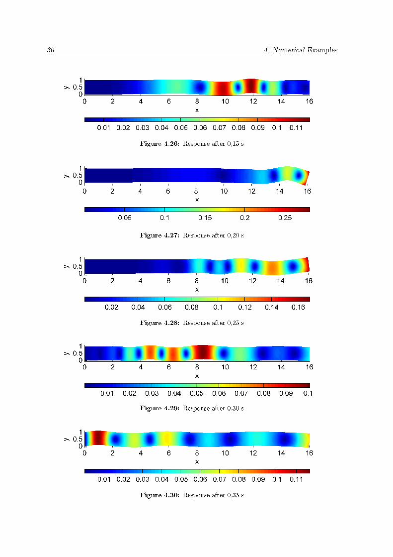
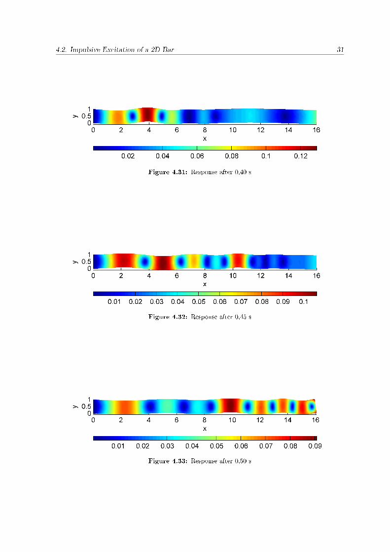
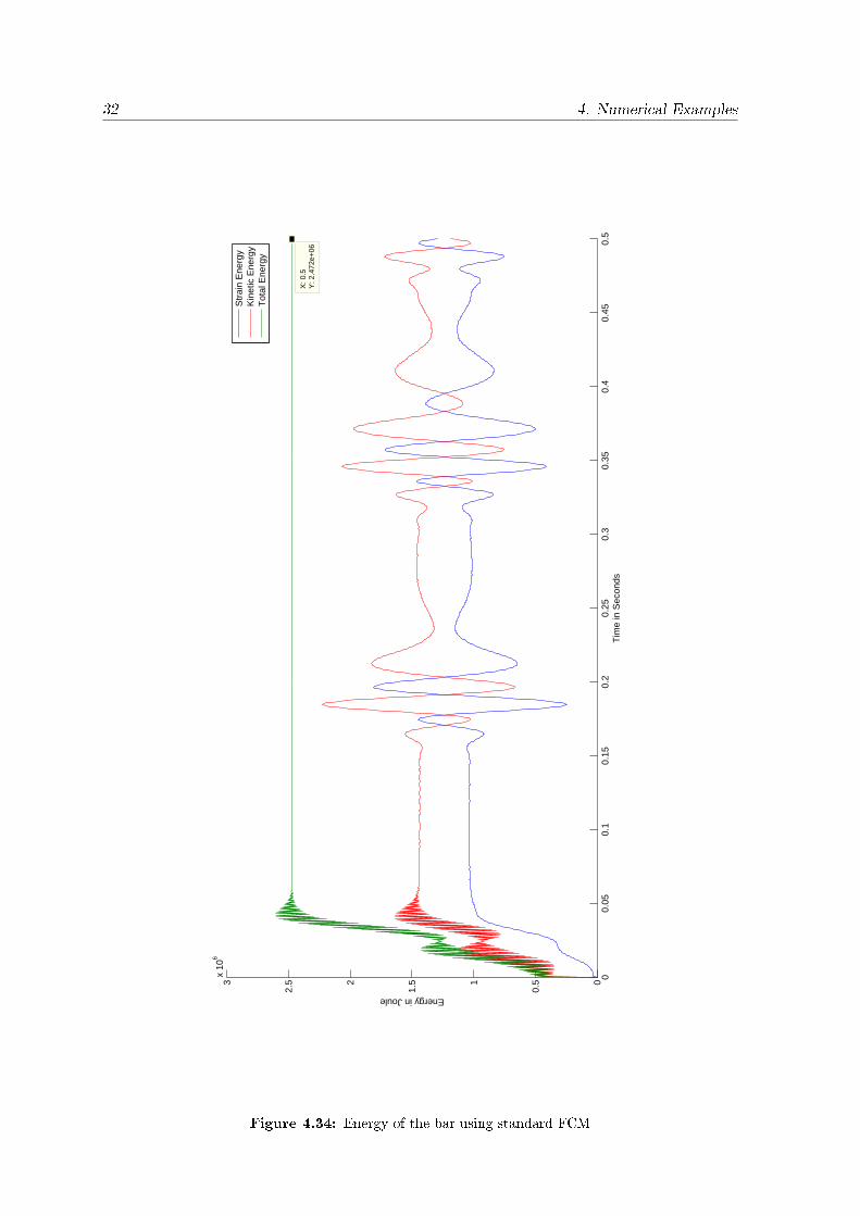
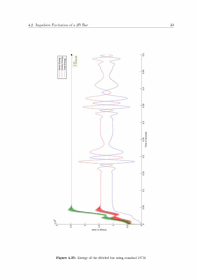
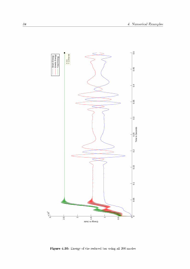
4.2 Impulsive Excitation of a 2D Bar
In the this section the kinetic, strain and total energy of a reduced bar is analyzed. There-fore, a bar with the same properties as in section 4.1 is considered (see gure 4.23). Justthe stimulation is now impulsive. This is realized by a Gauss Curve as Dirichlet boundarycondition. The response of the bar using the standard FCM is shown in gures 4.24 to 4.33.Furthermore, the energies of the undivided (gure 4.34) and divided (gure 4.35) bar usingthe standard FCM are plotted. The divided and undivided case result in the same energiescurves. Also the energies using the Craig-Bampton Method with all 200 modes is more orless equal to the energy using the standard FCM (gure 4.36). When reducing the number ofmodes, the total energy is also equal to the energy using standard FCM. But the strain andthe kinetic energy have increased oscillations (gure 4.37).
u(t) = 0.2 · exp(− (t−0.0245)2
2·0.012)
Super Element
Figure 4.23: Sketch of bar with super element
Figure 4.24: Response after 0,05 s
Figure 4.25: Response after 0,10 s
30 4. Numerical Examples
Figure 4.26: Response after 0,15 s
Figure 4.27: Response after 0,20 s
Figure 4.28: Response after 0,25 s
Figure 4.29: Response after 0,30 s
Figure 4.30: Response after 0,35 s
4.2. Impulsive Excitation of a 2D Bar 31
Figure 4.31: Response after 0,40 s
Figure 4.32: Response after 0,45 s
Figure 4.33: Response after 0,50 s
32 4. Numerical Examples
00.
050.
10.
150.
20.
250.
30.
350.
40.
450.
50
0.51
1.52
2.53
x 10
6
X: 0
.5Y
: 2.4
72e+
06
Tim
e in
Sec
onds
Energy in Joule
Str
ain
Ene
rgy
Kin
etic
Ene
rgy
Tot
al E
nerg
y
Figure 4.34: Energy of the bar using standard FCM
4.2. Impulsive Excitation of a 2D Bar 33
00.
050.
10.
150.
20.
250.
30.
350.
40.
450.
50
0.51
1.52
2.53
x 10
6
X: 0
.5Y
: 2.4
72e+
06
Tim
e in
sec
onds
Energy in Joule
Str
ain
Ene
rgy
Kin
etic
Ene
rgy
Tot
al E
nerg
y
Figure 4.35: Energy of the divided bar using standard FCM
34 4. Numerical Examples
00.
050.
10.
150.
20.
250.
30.
350.
40.
450.
50
0.51
1.52
2.53
x 10
6
X: 0
.5Y
: 2.4
72e+
06
Tim
e in
Sec
onds
Energy in Joule
Str
ain
Ene
rgy
Kin
etic
Ene
rgy
Tot
al E
nerg
y
Figure 4.36: Energy of the reduced bar using all 200 modes

4.2. Impulsive Excitation of a 2D Bar 35
00.
050.
10.
150.
20.
250.
30.
350.
40.
450.
50
0.51
1.52
2.53
x 10
6
X: 0
.5Y
: 2.4
72e+
06
Tim
e in
Sec
onds
Energy in Joule
Str
ain
Ene
rgy
Kin
etic
Ene
rgy
Tot
al E
nerg
y
Figure 4.37: Energy of the reduced bar using 5 modes
36 4. Numerical Examples
4.3 Finite Cell Method meets Craig-Bampton Method
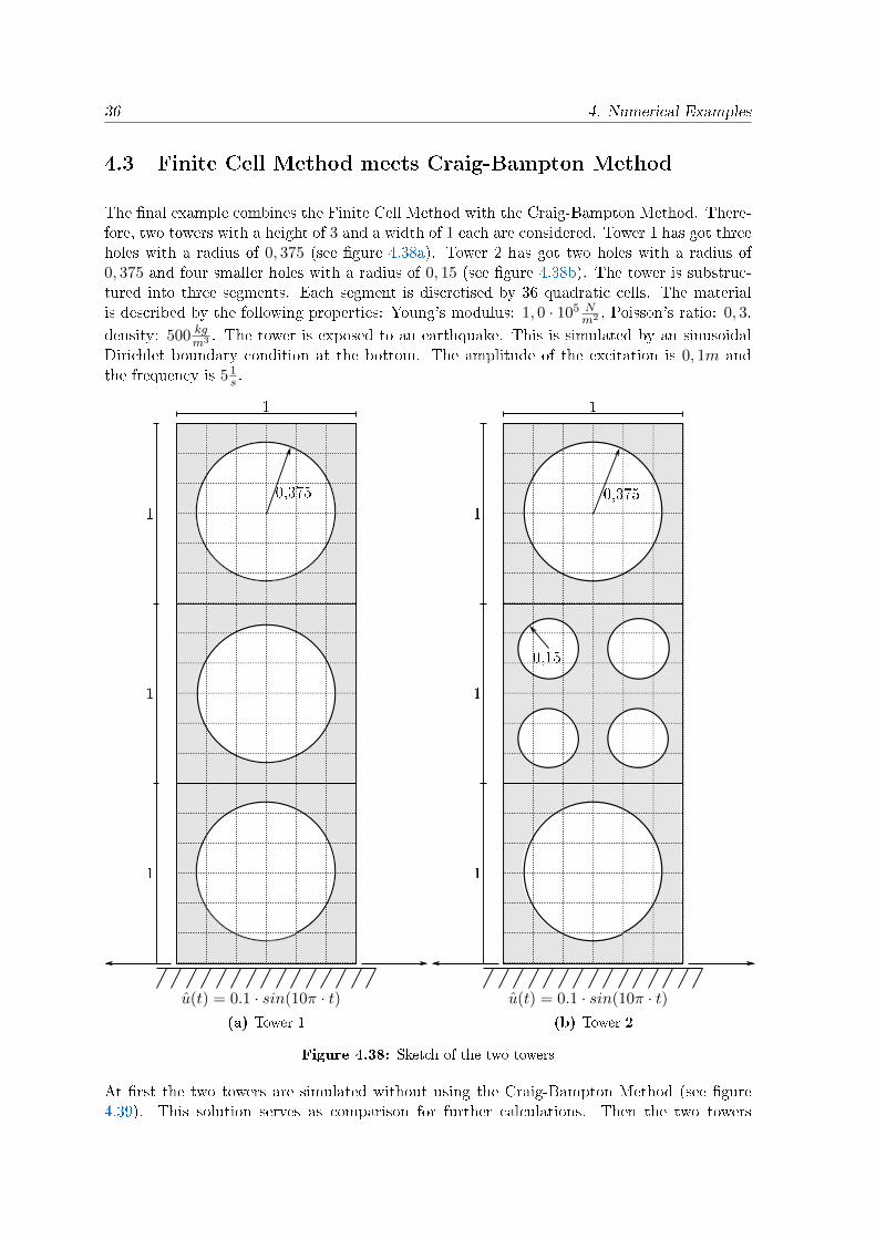
The nal example combines the Finite Cell Method with the Craig-Bampton Method. There-fore, two towers with a height of 3 and a width of 1 each are considered. Tower 1 has got threeholes with a radius of 0, 375 (see gure 4.38a). Tower 2 has got two holes with a radius of0, 375 and four smaller holes with a radius of 0, 15 (see gure 4.38b). The tower is substruc-tured into three segments. Each segment is discretised by 36 quadratic cells. The materialis described by the following properties: Young's modulus: 1, 0 · 105 N
m2 , Poisson's ratio: 0, 3,
density: 500 kgm3 . The tower is exposed to an earthquake. This is simulated by an sinusoidal
Dirichlet boundary condition at the bottom. The amplitude of the excitation is 0, 1m andthe frequency is 51
s .
u(t) = 0.1 · sin(10π · t)
0,375
1
1
1
1
(a) Tower 1
u(t) = 0.1 · sin(10π · t)
1
1
1
1
0,375
0,15
(b) Tower 2
Figure 4.38: Sketch of the two towers
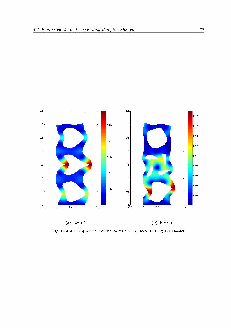
At rst the two towers are simulated without using the Craig-Bampton Method (see gure4.39). This solution serves as comparison for further calculations. Then the two towers
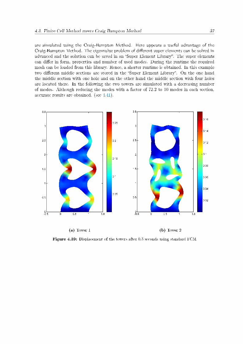
4.3. Finite Cell Method meets Craig-Bampton Method 37
are simulated using the Craig-Bampton Method. Here appears a useful advantage of theCraig-Bampton Method. The eigenvalue problem of dierent super elements can be solved inadvanced and the solution can be saved in an Super Element Library. The super elementscan dier in form, properties and number of used modes. During the runtime the requiredmesh can be loaded from this library. Hence, a shorter runtime is obtained. In this exampletwo dierent middle sections are stored in the Super Element Library. On the one handthe middle section with one hole and on the other hand the middle section with four holesare located there. In the following the two towers are simulated with a decreasing numberof modes. Although reducing the modes with a factor of 72.2 to 10 modes in each section,accurate results are obtained. (see 4.41).
(a) Tower 1 (b) Tower 2
Figure 4.39: Displacement of the towers after 0.5 seconds using standard FCM

38 4. Numerical Examples
(a) Tower 1 (b) Tower with six holes
Figure 4.40: Displacement of the towers after 0.5 seconds using all 3 · 722 modes
4.3. Finite Cell Method meets Craig-Bampton Method 39
(a) Tower 1 (b) Tower 2
Figure 4.41: Displacement of the towers after 0.5 seconds using 3 · 10 modes
40 4. Numerical Examples
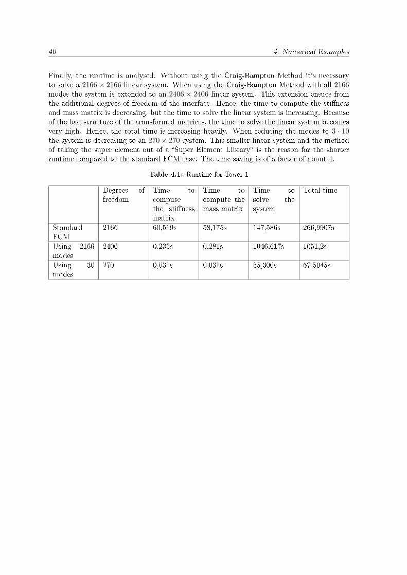
Finally, the runtime is analysed. Without using the Craig-Bampton Method it's necessaryto solve a 2166× 2166 linear system. When using the Craig-Bampton Method with all 2166modes the system is extended to an 2406 × 2406 linear system. This extension ensues fromthe additional degrees of freedom of the interface. Hence, the time to compute the stinessand mass matrix is decreasing, but the time to solve the linear system is increasing. Becauseof the bad structure of the transformed matrices, the time to solve the linear system becomesvery high. Hence, the total time is increasing heavily. When reducing the modes to 3 · 10the system is decreasing to an 270× 270 system. This smaller linear system and the methodof taking the super element out of a Super Element Library is the reason for the shorterruntime compared to the standard FCM case. The time saving is of a factor of about 4.
Table 4.1: Runtime for Tower 1
Degrees offreedom
Time tocomputethe stinessmatrix
Time tocompute themass matrix
Time tosolve thesystem
Total time
StandardFCM
2166 60,519s 58,175s 147,586s 266,9907s
Using 2166modes
2406 0,235s 0,281s 1046,617s 1051,2s
Using 30modes
270 0,031s 0,031s 65,300s 67,5045s
41
Chapter 5
Summary and Conclusions
This thesis combines the Finite Cell Method and the Craig-Bampton Method. Based onthe linear elastic equation the Finite Cell Method was introduced. The concepts of highorder shape functions, embedded domain and adaptive integration were described as themost important aspects of the method. In addition, the Penalty Method for weakly enforcedconstraints and the Newmark's Method were introduced. Afterwards the Craig-BamptonMethod was presented. Therefore, the transformation matrix was derived from the componentmode theory. Then the concept of substructuring was described.
In the context of the thesis the Craig-Bampton Method was implemented in the FCMLabMATLAB Toolbox, which was developed by the Chair for Computation in Engineering ofthe Technische Universität München. Therefore, the code was modied in order to supportmultiple meshes and the Nitsche's Method was integrated. Now, the advantages of both theCraig-Bampton Method and the Finite Cell Method are joined in the toolbox. After thedescription, how the method is integrated in the toolbox, various examples were simulated.It could be seen that very good results were obtained. Hence, a very useful combination oftwo powerful methods was created. The combined method obtains time savings during thepreprocessing because of the Finite Cell Method and during the solving process because ofthe Craig-Bampton Method.
The thesis only considered two-dimensional problems. A further step would be the extensionto 3D problems. An other point is the integration of the Nitsche's Method. The couplingof two standard FCM domains is already possible. In order to use it for the Craig-BamptonMethod, some modications have to be made. Explicitly a solution in order to couple 1Dand 2D domains is necessary. In the current version the martices, which are required for thismethod, don't match together. Finally the solver could be improved in order to obtain a betterruntime performance for matrices with the bad structure, resulting from the Craig-BamptonMethod.
In order to conclude, considerations for the industrial application are made. In the simulationprocess, for example in crash tests in the automative sector, dierent variants of a problemhave to be calculated. Only some parts are modied. Storing the unmodied parts with asuitable reduction in a Super Element Library, would safe a lot of time to solve complexproblems. Thus, substructuring could optimize and accelerate the simulation and developmentprocess.

42 5. Summary and Conclusions
LIST OF FIGURES 43
List of Figures
2.1 1D Legendre-based shape functions [22] . . . . . . . . . . . . . . . . . . . . . 6
2.2 Tensor-product structure of legendre-based shape functions [22] . . . . . . . . 7
2.3 Two dimensional mode types [22] . . . . . . . . . . . . . . . . . . . . . . . . . 7
2.4 The nite cell idea [17] [22] . . . . . . . . . . . . . . . . . . . . . . . . . . . . 8
2.5 Integration via space-trees [17] [22] . . . . . . . . . . . . . . . . . . . . . . . . 8
3.1 Sketch of a super element in the FCMLab MATLAB Toolbox . . . . . . . . . 16
3.2 Unreduced matrix structure . . . . . . . . . . . . . . . . . . . . . . . . . . . . 17
3.3 Reduced matrix structure . . . . . . . . . . . . . . . . . . . . . . . . . . . . . 17
3.4 Matrix structure of the whole example . . . . . . . . . . . . . . . . . . . . . . 18
4.1 Sketch of the bar . . . . . . . . . . . . . . . . . . . . . . . . . . . . . . . . . . 19
4.2 Response after 0,05 s . . . . . . . . . . . . . . . . . . . . . . . . . . . . . . . . 19
4.3 Response after 0,1 s . . . . . . . . . . . . . . . . . . . . . . . . . . . . . . . . 20
4.4 Response after 0,15 s . . . . . . . . . . . . . . . . . . . . . . . . . . . . . . . . 20
4.5 Response after 0,20 s . . . . . . . . . . . . . . . . . . . . . . . . . . . . . . . . 20
4.6 Response after 0,25 s . . . . . . . . . . . . . . . . . . . . . . . . . . . . . . . . 20
4.7 Response after 0,3 s . . . . . . . . . . . . . . . . . . . . . . . . . . . . . . . . 20
4.8 Response after 0,35 s . . . . . . . . . . . . . . . . . . . . . . . . . . . . . . . . 21
4.9 Response after 0,4 s . . . . . . . . . . . . . . . . . . . . . . . . . . . . . . . . 21
4.10 Response after 0,45 s . . . . . . . . . . . . . . . . . . . . . . . . . . . . . . . . 21
4.11 Response after 0,5 s . . . . . . . . . . . . . . . . . . . . . . . . . . . . . . . . 21
4.12 Response over time at the right free end . . . . . . . . . . . . . . . . . . . . . 22
4.13 Sketch of the divided bar . . . . . . . . . . . . . . . . . . . . . . . . . . . . . . 23

44 LIST OF FIGURES
4.14 Error of the divided bar at the right free end . . . . . . . . . . . . . . . . . . 23
4.15 Sketch of bar with super element . . . . . . . . . . . . . . . . . . . . . . . . . 23
4.16 Error of the bar at the right free end using all 200 modes . . . . . . . . . . . . 24
4.17 Error at the right free end using 100 modes . . . . . . . . . . . . . . . . . . . 24
4.18 Error at the right free end using 50 modes . . . . . . . . . . . . . . . . . . . . 25
4.19 Error at the right free end using 10 modes . . . . . . . . . . . . . . . . . . . . 25
4.20 Response after 0,5 s using few modes . . . . . . . . . . . . . . . . . . . . . . . 26
4.21 Time curve of the displacement at the sensor . . . . . . . . . . . . . . . . . . 27
4.22 Response using one of 200 modes . . . . . . . . . . . . . . . . . . . . . . . . . 28
4.23 Sketch of bar with super element . . . . . . . . . . . . . . . . . . . . . . . . . 29
4.24 Response after 0,05 s . . . . . . . . . . . . . . . . . . . . . . . . . . . . . . . . 29
4.25 Response after 0,10 s . . . . . . . . . . . . . . . . . . . . . . . . . . . . . . . . 29
4.26 Response after 0,15 s . . . . . . . . . . . . . . . . . . . . . . . . . . . . . . . . 30
4.27 Response after 0,20 s . . . . . . . . . . . . . . . . . . . . . . . . . . . . . . . . 30
4.28 Response after 0,25 s . . . . . . . . . . . . . . . . . . . . . . . . . . . . . . . . 30
4.29 Response after 0,30 s . . . . . . . . . . . . . . . . . . . . . . . . . . . . . . . . 30
4.30 Response after 0,35 s . . . . . . . . . . . . . . . . . . . . . . . . . . . . . . . . 30
4.31 Response after 0,40 s . . . . . . . . . . . . . . . . . . . . . . . . . . . . . . . . 31
4.32 Response after 0,45 s . . . . . . . . . . . . . . . . . . . . . . . . . . . . . . . . 31
4.33 Response after 0,50 s . . . . . . . . . . . . . . . . . . . . . . . . . . . . . . . . 31
4.34 Energy of the bar using standard FCM . . . . . . . . . . . . . . . . . . . . . . 32
4.35 Energy of the divided bar using standard FCM . . . . . . . . . . . . . . . . . 33
4.36 Energy of the reduced bar using all 200 modes . . . . . . . . . . . . . . . . . . 34
4.37 Energy of the reduced bar using 5 modes . . . . . . . . . . . . . . . . . . . . . 35
4.38 Sketch of the two towers . . . . . . . . . . . . . . . . . . . . . . . . . . . . . . 36
4.39 Displacement of the towers after 0.5 seconds using standard FCM . . . . . . . 37
4.40 Displacement of the towers after 0.5 seconds using all 3 · 722 modes . . . . . . 38
4.41 Displacement of the towers after 0.5 seconds using 3 · 10 modes . . . . . . . . 39

LIST OF TABLES 45
List of Tables
4.1 Runtime for Tower 1 . . . . . . . . . . . . . . . . . . . . . . . . . . . . . . . . 40

46 LIST OF TABLES

BIBLIOGRAPHY 47
Bibliography
[1] M. C. C. Bampton and R. R. Craig, Jr. Coupling of Substructures for Dynamic Analyses.AIAA Journal, 6(7):13131319, July 1968.
[2] R. D. Cook, D. S. Malkus, M. E. Plesha, and R. J. Witt. Concepts and Applications of
Finite Element Analysis. John Wiley & Sons, New York, NY, 4th ed. edition, 2002.
[3] R. R. Craig. Structural Dynamics: An Introduction to Computer Methods. John Wiley& Sons, New York, 1981.
[4] R. R. Craig and A. Kurdila. Fundamentals of Structural Dynamics. John Wiley, Hoboken,N.J, 2nd ed edition, 2006.
[5] A. Düster, J. Parvizian, Z. Yang, and E. Rank. The nite cell method for three-dimensional problems of solid mechanics. Computer Methods in Applied Mechanics and
Engineering, 197(4548):37683782, Aug. 2008.
[6] M. Elhaddad. Transient analysis with the nite cell method. Master's thesis, TechnischeUniversität München, Munich, 2014.
[7] S. Gordon. The Craig-Bampton Method, May 1999.
[8] M. Griebel and M. Schweitzer. A ParticlePartition of Unity Method Part V: Boundary
Conditions. Springer, Berlin, 2002.
[9] R. J. Guyan. Reduction of Stiness and Mass Matrices. AIAA Journal, vol. 3(no. 2):380,1965.
[10] T. J. R. Hughes. The Finite Element Method: Linear Static and Dynamic Finite Element
Analysis. Dover Publications, Mineola, NY, 2000.
[11] A. I. Özcan. A Nitsche-based mortar method for non-matching multi-patch discretizations
in the Finite Cell Method. Master's thesis, Technische Universität München, 2012.
[12] J. Parvizian, A. Düster, and E. Rank. Finite cell method. Computational Mechanics,41(1):121133, Apr. 2007.
[13] L. Pichler. Modal reduction and methods for ecient reliability assessmant in structural
dynamics. Number 341 in 11. VDI Verlag, Düsseldorf, 2010.
[14] E. Rank. Partial Dierential Equations: An Algorithmic Approach. Lecture notes,Technische Universität München, 2013.
48 BIBLIOGRAPHY
[15] E. Rank, S. Kollmannsberger, C. Sorger, and A. Düster. Shell Finite Cell Method: Ahigh order ctitious domain approach for thin-walled structures. Computer Methods in
Applied Mechanics and Engineering, 200(45-46):32003209, Oct. 2011.
[16] M. Ruchti. Model Simplication via Super Elements using the Finite Cell Method. Bach-elor's thesis, Technische Universität München, Chair for Computation in Engineering,Sept. 2013.
[17] D. Schillinger, M. Ruess, N. Zander, Y. Bazilevs, A. Düster, and E. Rank. Small andlarge deformation analysis with the p- and B-spline versions of the nite cell method.Computational Mechanics, 50(4):445478, Feb. 2012.
[18] B. A. Szabó and I. Babuska. Finite Element Analysis. John Wiley & Sons, New York,1991.
[19] W. A. Wall and A. Popp. Computational Solid Dynamics (MSE). Lecture notes, Institutfor Computational Mechanics, Technische Universität München, 2012.
[20] E. Woschke, C. Daniel, and J. Strackeljan. Reduktion elastischer Strukturen für MKSAnwendungen. Technical report, Otto-von-Guericke-Universität, Magdeburg, 2007.
[21] J. T. Young and W. B. Haile. Primer on the Craig-Bampton Method. Technical report,June 2000.
[22] N. Zander, T. Bog, M. Elhaddad, R. Espinoza, H. Hu, A. Joly, C. Wu, P. Zerbe,A. Düster, S. Kollmannsberger, J. Parvizian, M. Ruess, D. Schillinger, and E. Rank.FCMLab: a nite cell research toolbox for MATLAB. Advances in Engineering Soft-
ware, 74:4963, Aug. 2014.