Embed Size (px)
Citation preview
Department of Precision and Microsystems Engineering
Experimental dynamic substructuringusing direct time-domain deconvolvedimpulse response functions
T. van der HorstReport no : EM 2014.001Coaches : ir. P.L.C. van der Valk and ir. M.V. van der SeijsProfessor : prof. dr. ir. A. van KeulenSpecialisation : Engineering MechanicsType of report : MSc. thesisDate : February 14, 2014

Abstract
The dynamics of systems can be analysed by combining the dynamics of its compo-nents. This method is generally known as dynamic substructuring. It allows for efficientcomputation of the dynamics of structures that would otherwise be to complex to de-termine. Most dynamic substructuring approaches use the frequency domain for there-assembling of the subcomponents. Recently, a different implementation of the dy-namic substructuring method has been introduced: impulse based substructuring (IBS).It uses impulse response function in the time-domain for representing the dynamics ofthe subcomponents, obtained by numerical models or experimental testing. Comparedto the frequency domain methods, the impulse based substructuring scheme proves tobe advantageous when analysing the high-frequency characteristics of a system. Thehigh-frequency dynamics are excited when the system is subjected to blasts, shocks orimpulsive loading. Due to the sensitivity of the impulse based substructure scheme,experimentally obtained impulse response functions can not be used for describing thedynamics of a subsystem.
The focus of this thesis is developing a direct time-domain technique for determiningthe experimental impulse response. This is realised by introducing the inverse finiteimpulse response force filter, which operates independent of the output system response.This time-domain approach will avoid frequency domain induced errors, i.e. windowing,anti-aliasing and Fourier transforms, in the effort of determining a highly accurate im-pulse response functions. The quality of the time-domain acquired impulse response, aswell as the measurement induced errors are tested on the impulse based substructuringscheme. The procedures are illustrated by application to an one-dimensional bar.
The inverse force filter is successful in finding the experimental (averaged) impulseresponse. The accuracy of the filter depends on the length of the filter and the condition-ing of the force auto correlation matrix. The eigenvalue decomposition of this matrix ledto the formulation of a selection criteria between replicate measurements and a filteringoperation. The inverse filter can also be defined by using a Fourier transform and itsinverse. If both methods are compared, it is shown that the time-domain approach isless accurate and time efficient.
The direct time-domain approach did not change the impulse response in such anextend that coupling by the impulse based substructuring scheme was possible. Sincecoupling between numerically simulated data is possible, measurement errors are intro-duced on the impulse response functions to test their sensitivity to the IBS scheme. Itis observed that a small error on the exponential decay, of the perfect impulse response,directly resulted in uncoupled full system responses. This led to the identification of themodal parameters of the measurement to get rid of these amplitude errors, by means ofthe least squares complex exponential method. The perfect synthesised impulse responseare successful in finding a coupled full system response.
Experimental dynamic substructuring only finds the full coupled response if a cleansynthesised impulse response function of the subcomponents is used. It can also beconcluded that the inverse filter is not as accurate as its frequency domain counterpart.However, the inverse force filter will make deconvolution of small parts of the outputresponse possible. This is desirable when testing lightly damped structures.
I


Contents
Abstract III
Notation VI
1 Introduction 11.1 Research context . . . . . . . . . . . . . . . . . . . . . . . . . . . . . . . . . . . . 11.2 Research goal . . . . . . . . . . . . . . . . . . . . . . . . . . . . . . . . . . . . . . 1
1.2.1 System description . . . . . . . . . . . . . . . . . . . . . . . . . . . . . . . 21.3 Thesis outline . . . . . . . . . . . . . . . . . . . . . . . . . . . . . . . . . . . . . . 2
2 Impulse response 52.1 Introduction . . . . . . . . . . . . . . . . . . . . . . . . . . . . . . . . . . . . . . . 52.2 Linear time-invariant systems . . . . . . . . . . . . . . . . . . . . . . . . . . . . . 5
2.2.1 Convolution properties . . . . . . . . . . . . . . . . . . . . . . . . . . . . . 62.3 Time response of dynamical systems . . . . . . . . . . . . . . . . . . . . . . . . . 72.4 Experimental dynamics and deconvolution . . . . . . . . . . . . . . . . . . . . . . 8
2.4.1 Measurement of POM bar . . . . . . . . . . . . . . . . . . . . . . . . . . . 92.5 Impulse response simulation . . . . . . . . . . . . . . . . . . . . . . . . . . . . . . 11
2.5.1 Newmark time integration . . . . . . . . . . . . . . . . . . . . . . . . . . . 112.5.2 Modal synthesis . . . . . . . . . . . . . . . . . . . . . . . . . . . . . . . . 12
3 Time-domain deconvolution 153.1 Introduction . . . . . . . . . . . . . . . . . . . . . . . . . . . . . . . . . . . . . . . 153.2 Linear least-square system . . . . . . . . . . . . . . . . . . . . . . . . . . . . . . . 153.3 Inverse force filter . . . . . . . . . . . . . . . . . . . . . . . . . . . . . . . . . . . 17
3.3.1 Inverse FIR filter of non-perfect impact . . . . . . . . . . . . . . . . . . . 183.3.2 Impulse response reconstruction . . . . . . . . . . . . . . . . . . . . . . . 18
3.4 Auto-correlation matrix . . . . . . . . . . . . . . . . . . . . . . . . . . . . . . . . 193.4.1 Signal separation . . . . . . . . . . . . . . . . . . . . . . . . . . . . . . . . 20
3.5 Time domain averaging . . . . . . . . . . . . . . . . . . . . . . . . . . . . . . . . 223.5.1 Response function estimators . . . . . . . . . . . . . . . . . . . . . . . . . 223.5.2 Multiple input IRF estimation . . . . . . . . . . . . . . . . . . . . . . . . 23
3.6 Method validation . . . . . . . . . . . . . . . . . . . . . . . . . . . . . . . . . . . 243.7 Summary . . . . . . . . . . . . . . . . . . . . . . . . . . . . . . . . . . . . . . . . 25
4 Dynamic substructuring using impulse response functions 294.1 Introduction . . . . . . . . . . . . . . . . . . . . . . . . . . . . . . . . . . . . . . . 294.2 Impulse based substructuring . . . . . . . . . . . . . . . . . . . . . . . . . . . . . 29
4.2.1 Assembly of impulse responses . . . . . . . . . . . . . . . . . . . . . . . . 30
III

IV Contents
4.3 Substructuring with numerical models . . . . . . . . . . . . . . . . . . . . . . . . 314.3.1 Newmark time integration . . . . . . . . . . . . . . . . . . . . . . . . . . . 314.3.2 Modal synthesis . . . . . . . . . . . . . . . . . . . . . . . . . . . . . . . . 31
4.4 Substructuring with experimental data . . . . . . . . . . . . . . . . . . . . . . . . 334.5 Summary . . . . . . . . . . . . . . . . . . . . . . . . . . . . . . . . . . . . . . . . 34
5 Strategies for improving experimental IRF’s for dynamic substructuring 355.1 Introduction . . . . . . . . . . . . . . . . . . . . . . . . . . . . . . . . . . . . . . . 355.2 Exploratory research . . . . . . . . . . . . . . . . . . . . . . . . . . . . . . . . . . 355.3 Hybrid substructuring . . . . . . . . . . . . . . . . . . . . . . . . . . . . . . . . . 375.4 Substructuring sensitivity analysis . . . . . . . . . . . . . . . . . . . . . . . . . . 37
5.4.1 Influence of noise . . . . . . . . . . . . . . . . . . . . . . . . . . . . . . . . 385.4.2 Re-sampling and filtering . . . . . . . . . . . . . . . . . . . . . . . . . . . 385.4.3 Change underlying dynamics . . . . . . . . . . . . . . . . . . . . . . . . . 395.4.4 Exponential decay . . . . . . . . . . . . . . . . . . . . . . . . . . . . . . . 40
5.5 Modal fit . . . . . . . . . . . . . . . . . . . . . . . . . . . . . . . . . . . . . . . . 415.6 Summary . . . . . . . . . . . . . . . . . . . . . . . . . . . . . . . . . . . . . . . . 45
6 Conclusions and recommendations 476.1 Conclusions . . . . . . . . . . . . . . . . . . . . . . . . . . . . . . . . . . . . . . . 476.2 Recommendations . . . . . . . . . . . . . . . . . . . . . . . . . . . . . . . . . . . 48
6.2.1 Outlook . . . . . . . . . . . . . . . . . . . . . . . . . . . . . . . . . . . . . 48
Bibliography 51
A Inverse force filter 53A.1 Implementation . . . . . . . . . . . . . . . . . . . . . . . . . . . . . . . . . . . . . 53A.2 Averaged comparison . . . . . . . . . . . . . . . . . . . . . . . . . . . . . . . . . . 54
B Impulse based substructuring 55
C Least-squares complex exponential 57C.1 Stabilisation diagram . . . . . . . . . . . . . . . . . . . . . . . . . . . . . . . . . . 58
D Response truncation 59

Notation
SymbolsGeneral meaning of often used symbols, unless otherwise noted in context:
B Signed Boolean assembly matrix L Length of subsystemC Damping matrix M Sample length inputd Diameter M Mass matrixE Young’s modulus N Sample length outputf Force filter array Q Sample length impulse responsef inv Inverse force filter r Auto-correlationF Force filter Toeplitz matrix R Auto-correlation matrixF inv Pseudo inverse Force Toeplitz matrix S Time stepping matrixF Fourier transform t Timeg Connection force array u Output displacement fieldG Spectral density matrix V Eigenvector matrixh Impulse response array x Vibration modeH Impulse response matrix ˙ ConvolutionK Stiffness matrix ‹ Correlation
Greek symbols:
β,γ Newmark time integration parameters µ Modal massδ Unit Impulse ρ Density∆ Step increment ω Circular frequency or eigenfrequencyε Amplitude error ωd Damped eigenfrequencyλ Lagrange multipliers ζ Damping ratioΛ Eigenvalue matrix
Subscripts and superscripts:
‚ Averaged matrix 9‚ First time derivative‚ Complex conjugate ‚ Prediction array‚psq Component of substructure s ‚: Pseudo inverse of matrix‚x DoF at position x :‚ Second time derivative
AbbreviationsDFT Discrete Fourier transform FRF Frequency response functionDoF Degrees of freedom IDFT Inverse discrete Fourier transformFIR Finite impulse response IRF Impulse response function
V


Chapter 1
Introduction
1.1 Research contextThe modern engineer is faced with structures that are becoming lighter and increasingly morecomplex. This calls for efficient solving of the structural dynamics of any product, which is essen-tial for quantifying its performance. Dynamic fragmentation allows efficient analysis of complexstructures, as the dynamic behaviour of smaller and simpler structural fragments (substructures)are generally easier to determine. The possibilities of sharing and combining substructures fromdifferent design groups, combining experimentally and numerically obtained dynamics and theoptimisation of a single subcomponent without the need for a full analysis, adds to the effi-ciency. Most methods which utilise this dynamic fragmentation, use the frequency domain forthe re-assembly of the substructures into the full system model [5].
The frequency domain based substructuring method is however badly suited for represent-ing the response to impact like excitations, i.e. blast, shock and impulsive loading, and thelarge frequency band makes this strategy also expensive. Obtaining usable measured frequencyresponse functions, associated with those excitations, is a delicate process. The response is onlyobtained through several processing steps, i.e. windowing, anti-aliasing and Fourier transforms,which will unavoidably alter the information contained in the measurement. Nevertheless, theevaluation of the performance of a product subjected to this loading is essential, take for exam-ple the landing gear of an aircraft, handheld electronic devices that are dropped or a gun whenfiring. This led to the formulation of a transient dynamic substructuring counterpart [7, 11]. Ituses impulse response functions, which are better suited for simulating these broadband loads.
In the design stages of these products, its performance to impact is analysed by assemblingthe impulse response functions of the substructures from an existing database or newly computedor measured data. The impulse based substructuring scheme is advantages over its frequencydomain counterpart, in the ability to couple the dynamics of linear models and measurementsto non-linear models [13]. This design methodology will improve the quality and design cycletime of every new product.
1.2 Research goalThe above presented design methodology, made possible by the impulse based substructuringscheme, is very attractive. The quality of the full system response will depend on the quality ofthe individual impulse response functions representing the true dynamics of the subcomponents.An accurate way of determining the linear dynamics of a component is by means of experimentaltesting.
1

2 1.3. Thesis outline
To date, it is not possible to use measured impulse response functions in the impulse basedsubstructuring scheme for finding stable and coupled full system responses. This exploratoryresearch thesis pursues the objective of
Improvements on the impulse response computation and determining the sensitivity ofmeasurement induced errors on the impulse based substructuring scheme.
Impact testing is widely used, but the non perfect impulse demands a deconvolution op-eration between the output response and the input force. Traditionally the impulse responseis obtained through the frequency domain and consequently suffers from frequency domain in-duced errors as presented in section 1.1. The idea for a more natural time-domain deconvolvedimpulse response was presented in [10], but the computational cost of inverting large matricesinherent to impact testing leaves room for improvements. An inverse finite impulse response(FIR) force filter is introduced, which operates independent of the output response. The qualityof the time-domain deconvolved impulse response functions, as well as the measurement inducederrors are tested on the impulse based substructuring scheme. The procedures are illustratedby application to an one-dimensional bar.
1.2.1 System description
The dynamic substructuring analysis using time-domain deconvolved impulse response func-tions is tested on the one-dimensional polyoxymethylene (POM) bar [10], which is assumed tobehave linearly. This one dimensional academical example was chosen for the easy of numericalmodelling, coupling and result interpretation. The full reference system is a bar with length 2L,as sketched in figure 1.1. The bar with free floating boundary conditions is excited with force fat its left end face. This bar is now divided into two subsystems of equal length. The impulseresponse functions and the introduction of a force at the interface degrees of freedom makes itpossible to assemble the subsystems into the full model.
Id
2L
9up1q0 9up1qL 9up2q0 9up2qLλ
gp1qL
L
f
9upfullq0 9upfullq2L
L gp2q0
f
(a) The bar and the division in subsystems
d [mm] L [mm] ρ [kg/m3] E [GPa]
40 475.75 1420 3.75
(b) Dimensions and material properties
Figure 1.1: Schematic view of the POM bar with all the necessary parameters for the dynamicsubstructuring process. The black dots indicate the interface degrees of freedom.
1.3 Thesis outlineIn this thesis, a time-domain deconvolution operation is presented for finding the impulse re-sponse out of multiple measurements. A selection criteria between multiple measurements and afiltering operation are also included in this time-domain approach. The quality of the measuredimpulse response is defined by comparing it to numerical models. These differences are used ina sensitivity analysis of the measurement induced errors on the dynamic substructuring scheme.
In figure 1.2, the workflow of the thesis is schematically shown and the chapters associatedwith each topic are indicated. Chapter 2 introduces the reader to the impulse response. The im-pulse response is obtained either by solving the equations of motions or by experimental testing

Chapter 1. Introduction 3
ImpulseresponsfunctionChapter 3
ExperimentSection 2.4
Subsystem
Numericalmodel
Section 2.5
LSCE fitSection 5.5
Newmark
Modalsynthesis
Modalsynthesis
Impulsebased sub-structuringChapter 4
Hybridmodel
Section 5.3
Coupledsystem?
Uncertaintyquantifi-cation
Section 5.4
Figure 1.2: Schematic representation of thesis content in a flowchart.
and performing the deconvolution operation. In chapter 3, a direct time-domain deconvolutionoperation is presented by introduction of the inverse force filter. Operations that are convention-ally associated with the frequency domain, i.e. signal filtering, the auto power spectral densityand averaging, are presented in their time-domain counterparts. This chapter concludes with themethod validation of the inverse force filter. Chapter 4 introduces the interface problem, whichmakes the coupling between substructures possible. The impulse based substructuring schemeis tested with Newmark time integrated, modal synthesised and experimental impulse responsefunctions. In chapter 5, multiple operations are explored in the effort of coupling measuredimpulse response functions. Also, some of the experimental induced errors are represented byaltering perfect response functions, to see their influence on the dynamic substructuring scheme.

Chapter 2
Impulse response
2.1 Introduction
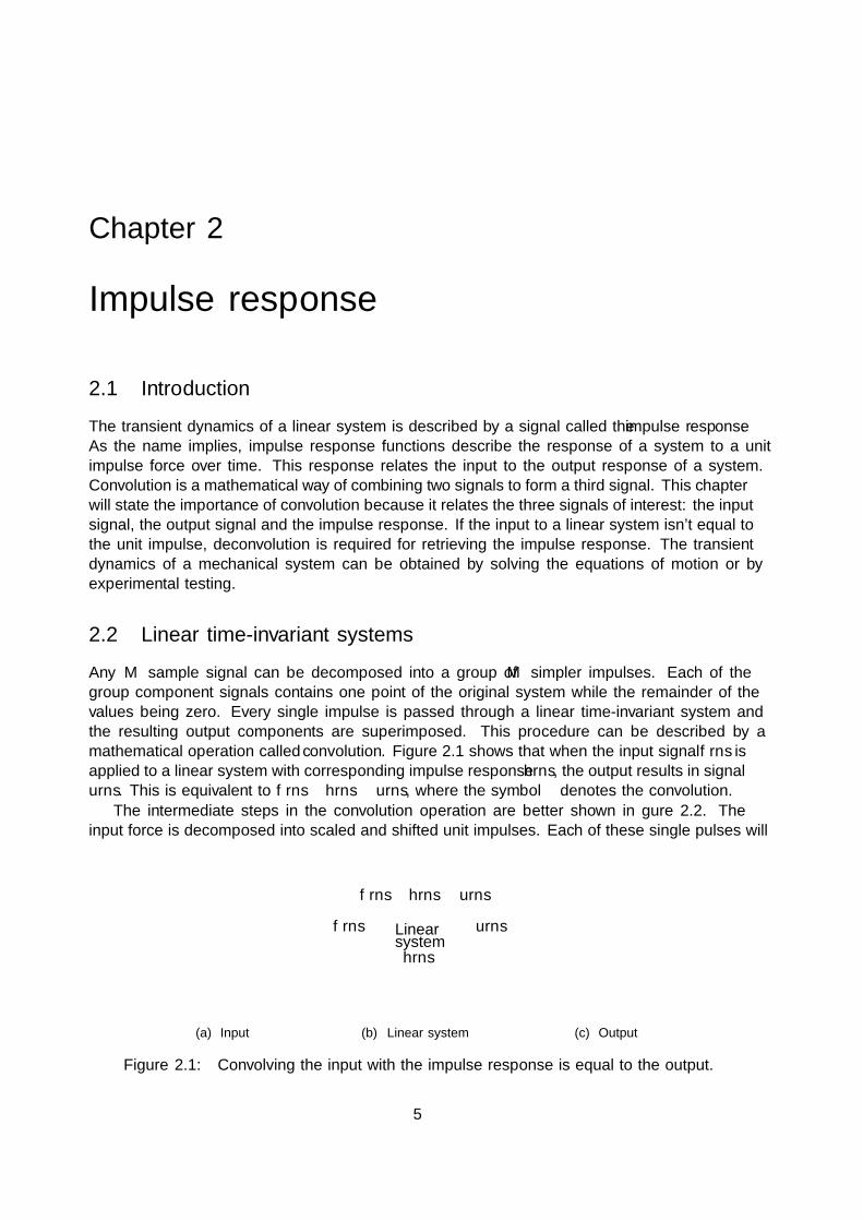
The transient dynamics of a linear system is described by a signal called the impulse response.As the name implies, impulse response functions describe the response of a system to a unitimpulse force over time. This response relates the input to the output response of a system.Convolution is a mathematical way of combining two signals to form a third signal. This chapterwill state the importance of convolution because it relates the three signals of interest: the inputsignal, the output signal and the impulse response. If the input to a linear system isn’t equal tothe unit impulse, deconvolution is required for retrieving the impulse response. The transientdynamics of a mechanical system can be obtained by solving the equations of motion or byexperimental testing.
2.2 Linear time-invariant systems
Any M sample signal can be decomposed into a group of M simpler impulses. Each of thegroup component signals contains one point of the original system while the remainder of thevalues being zero. Every single impulse is passed through a linear time-invariant system andthe resulting output components are superimposed. This procedure can be described by amathematical operation called convolution. Figure 2.1 shows that when the input signal f rns isapplied to a linear system with corresponding impulse response hrns, the output results in signalurns. This is equivalent to f rns˙ hrns “ urns, where the symbol ˙ denotes the convolution.
The intermediate steps in the convolution operation are better shown in figure 2.2. Theinput force is decomposed into scaled and shifted unit impulses. Each of these single pulses will
0 1 2 3 40
0.5
1
samples [n]
f[n
]
(a) Input
Linearsystemhrns
f rns urnsf rns˙ hrns “ urns
(b) Linear system
0 5 100
0.51
1.5
samples [n]
u[n
]
(c) Output
Figure 2.1: Convolving the input with the impulse response is equal to the output.
5

6 2.2. Linear time-invariant systems
generate shifted and scaled impulse responses and if all these responses are superimposed, theoutput response is found. If the impulse response of the system is known, the output can becalculated for any input signal.
01
23
t0
0
1
OtherLabel
delay rτ sÐÝtime rss
f[N
] impulse response h
input force f
output response u
outp
utre
sp.
[m/s
2 ]
Figure 2.2: Example of the convolution operation. The force signal f is decomposed into a setof scaled and shifted unit impulses: fpτqδpt´ τq. The first decomposed impulse isindeed the unit impulse δ, which makes the output equal to the impulse response h.The other three impulses also result in shifted and scaled functions of the impulseresponse. If the four shifted and scaled impulse responses are superimposed, theoutput response u is obtained.
2.2.1 Convolution properties
Some of the useful properties of convolution, which will be used later in this thesis, are listedbelow.
• The most simple input is the unit impulse and is symbolized by δrns. The unit impulsefunction shown in figure 2.3a is a Dirac delta impulse with the following properties:
δrns#
1 if n “ 00 otherwise
(2.1)
and will give direct access to the impulse response if it is the input to the system, accordingto figure 2.3. This property makes the unit delta function the identity for convolution.
• The commutative property for convolution states that the input and impulse response canbe changed, without changing the output.
f rns˙ hrns “ hrns˙ f rns “ urns (2.2)
This will turn out to be a useful mathematical property but does not have any physicalmeaning.
• As shown in figure 2.1, an input signal f rns enters a linear system with an impulse responsehrns, resulting in an output signal urns. If M and Q are respectively the sample lengthsof f rns and hrns, than the output signal urns, resulting from this convolution operation,consists of N “M `Q´ 1 samples.
Chapter 2. Impulse response 7
0 2 4 60
0.5
1
samples [n]
δ[n]
(a) Unit impulse
Linearsystem
δrns hrnsδrns˙ hrns “ hrns
(b) Linear system
0 2 4 6´1012
samples [n]
h[n
]
(c) Impulse response
Figure 2.3: Unit delta function as the input for a linear system and the output is the impulseresponse.
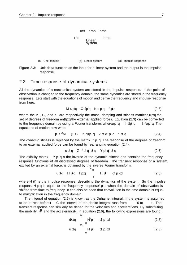
2.3 Time response of dynamical systemsAll the dynamics of a mechanical system are stored in the impulse response. If the point ofobservation is changed to the frequency domain, the same dynamics are stored in the frequencyresponse. Lets start with the equations of motion and derive the frequency and impulse responsefrom here.
M :uptq `C 9uptq `Kuptq “ fptq (2.3)
where the M , C, and K are respectively the mass, damping and stiffness matrices, uptq theset of degrees of freedom and fptq the external applied forces. Equation (2.3) can be convertedto the frequency domain by using a Fourier transform, where :upωq “ jω 9upωq “ ´ω2upωq. Theequations of motion now write:
p´ω2M ` jωC `Kqupωq “ Zpωqupωq “ fpωq (2.4)
The dynamic stiffness is replaced by the matrix Zpωq. The response of the degrees of freedomto an external applied force can be found by rearranging equation (2.4).
upωq “ Z´1pωqfpωq “ Y pωqfpωq (2.5)
The flexibility matrix Y pωq is the inverse of the dynamic stiffness and contains the frequencyresponse functions of all discretised degrees of freedom. The transient response of a system,excited by an external force, is obtained by the inverse Fourier transform:
uptq “Hptq˙ fptq “ż 8
τ“´8Hpt´ τqfpτqdτ (2.6)
where H(t) is the impulse response, describing the dynamics of the system. So the impulseresponse Hptq is equal to the frequency response Y pωq when the domain of observation isshifted from time to frequency. It can also be seen that convolution in the time domain is equalto multiplication in the frequency domain.
The integral of equation (2.6) is known as the Duhamel integral. If the system is assumedto be at rest before t “ 0, the interval of the definite integral runs from τ “ 0 to τ “ t. Thetransient response can similarly be defined for the velocities and accelerations. By substitutingthe mobility 9H and the accelerance :H in equation (2.6), the following expressions are found:
9uptq “ż t
τ“09Hpt´ τqfpτqdτ (2.7)
:uptq “ż t
τ“0:Hpt´ τqfpτqdτ (2.8)
8 2.4. Experimental dynamics and deconvolution
The output response at time t can be interpret as an infinite sum of the impulse responses tothe infinitesimal impulses fpτqdτ before time t. In this notation, each impulse at time τ givesa contribution through the flipped impulse response, so from t to τ .
2.4 Experimental dynamics and deconvolution
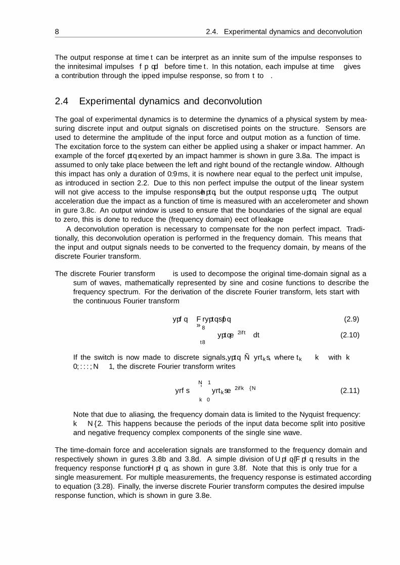
The goal of experimental dynamics is to determine the dynamics of a physical system by mea-suring discrete input and output signals on discretised points on the structure. Sensors areused to determine the amplitude of the input force and output motion as a function of time.The excitation force to the system can either be applied using a shaker or impact hammer. Anexample of the force fptq exerted by an impact hammer is shown in figure 3.8a. The impact isassumed to only take place between the left and right bound of the rectangle window. Althoughthis impact has only a duration of 0.9ms, it is nowhere near equal to the perfect unit impulse,as introduced in section 2.2. Due to this non perfect impulse the output of the linear systemwill not give access to the impulse response hptq, but the output response uptq. The outputacceleration due the impact as a function of time is measured with an accelerometer and shownin figure 3.8c. An output window is used to ensure that the boundaries of the signal are equalto zero, this is done to reduce the (frequency domain) effect of leakage.
A deconvolution operation is necessary to compensate for the non perfect impact. Tradi-tionally, this deconvolution operation is performed in the frequency domain. This means thatthe input and output signals needs to be converted to the frequency domain, by means of thediscrete Fourier transform.
The discrete Fourier transform is used to decompose the original time-domain signal as asum of waves, mathematically represented by sine and cosine functions to describe thefrequency spectrum. For the derivation of the discrete Fourier transform, lets start withthe continuous Fourier transform
ypfq “ Fryptqspfq (2.9)
“ż 8
t“´8yptqe´2iπft dt (2.10)
If the switch is now made to discrete signals, yptq Ñ yrtks, where tk “ k∆ with k “0, . . . , N ´ 1, the discrete Fourier transform writes
yrf s “N´1ÿ
k“0yrtkse´2πifk{N (2.11)
Note that due to aliasing, the frequency domain data is limited to the Nyquist frequency:k “ N{2. This happens because the periods of the input data become split into positiveand negative frequency complex components of the single sine wave.
The time-domain force and acceleration signals are transformed to the frequency domain andrespectively shown in figures 3.8b and 3.8d. A simple division of Upωq{F pωq results in thefrequency response function Hpωq, as shown in figure 3.8f. Note that this is only true for asingle measurement. For multiple measurements, the frequency response is estimated accordingto equation (3.28). Finally, the inverse discrete Fourier transform computes the desired impulseresponse function, which is shown in figure 3.8e.
Chapter 2. Impulse response 9
48 49 50 51 520
200400600800
time [ms]
forc
e[N
]
(a) Input fptq and window
DFTùñ
0 8000 16000
10´2
100
frequency [Hz]
forc
e[N
]
(b) Input F pωq
50 55 60´500
0
500
1000
time [ms]
acce
lera
tion
[m/s
2 ]
(c) Output uptq and window
DFTùñ
0 8000 16000
10´2
100
frequency [Hz]ac
cele
ratio
n[m
/s2 ]
(d) Output Upωq
ó hptq “ finvptq˙ uptq
0 2 4´4´2
024
time [ms]
IR[m
/s2 /N
]
(e) Impulse response hptq
IDFTðù
óHpωq “ UpωqF pωq
0 8000 16000
10´1
101
frequency [Hz]
FR[m
/s2 /N
]
(f) Frequency response Hpωq
Figure 2.4: Flowchart showing two paths (red and green) from the input and output responseto the impulse response. Left the time and right the frequency domain.
2.4.1 Measurement of POM bar
The force input and the velocity output are measured on the locations given in figure 1.1a.First, the homogeneous full bar was measured before the subsystems were cut to length, suchthat the reference configuration had no additional joint stiffness and damping. The gatheredexperimental data will be used in chapter 3 to test the proposed deconvolution operation andin chapter 4 to couple the substructures into the full system.
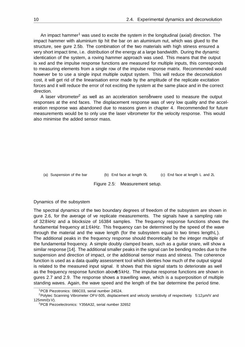
The bar is supported by a lightly inflated bike inner tube to represent the free floatingboundary conditions, as shown in figure 2.5a. The suspension of the bar is not ideal since itintroduces some systematic error into the measurement, i.g. the system is more damped, therigid body mode is no longer at zero hertz and the induced moment around the inner tubeintroduces bending modes.
10 2.4. Experimental dynamics and deconvolution
An impact hammer1 was used to excite the system in the longitudinal (axial) direction. Theimpact hammer with aluminium tip hit the bar on an aluminium nut, which was glued to thestructure, see figure 2.5b. The combination of the two materials with high stiffness ensured avery short impact time, i.e. distribution of the energy at a large bandwidth. During the dynamicidentification of the system, a roving hammer approach was used. This means that the outputis fixed and the impulse response functions are measured for multiple inputs, this correspondsto measuring elements from a single row of the impulse response matrix. Recommended wouldhowever be to use a single input multiple output system. This will reduce the deconvolutioncost, it will get rid of the linearisation error made by the amplitude of the replicate excitationforces and it will reduce the error of not exciting the system at the same place and in the correctdirection.
A laser vibrometer2 as well as an acceleration sensor3 were used to measure the outputresponses at the end faces. The displacement response was of very low quality and the accel-eration response was abandoned due to reasons given in chapter 4. Recommended for futuremeasurements would be to only use the laser vibrometer for the velocity response. This wouldalso minimise the added sensor mass.
(a) Suspension of the bar (b) End face at length 0L (c) End face at length L and 2L
Figure 2.5: Measurement setup.
Dynamics of the subsystem
The spectral dynamics of the two boundary degrees of freedom of the subsystem are shown infigure 2.6, for the average of five replicate measurements. The signals have a sampling rateof 32.8 kHz and a blocksize of 16384 samples. The frequency response functions shows thefundamental frequency at 1.6 kHz. This frequency can be determined by the speed of the wavethrough the material and the wave length (for the subsystem equal to two times length L).The additional peaks in the frequency response should theoretically be the integer multiple ofthe fundamental frequency. A simple doubly clamped beam, such as a guitar snare, will show asimilar response [14]. The additional smaller peaks in the signal can be bending modes due to thesuspension and direction of impact, or the additional sensor mass and stiffness. The coherencefunction is used as a data quality assessment tool which identifies how much of the output signalis related to the measured input signal. It shows that this signal starts to deteriorate as wellas the frequency response function above 6.5 kHz. The impulse response functions are shown infigures 2.7 and 2.9. The response shows a travelling wave, which is a superposition of multiplestanding waves. Again, the wave speed and the length of the bar determine the period time.
1PCB Piezotronics: 086C03, serial number 24524.2Polytec Scanning Vibrometer OFV-505, displacement and velocity sensitivity of respectively 5.12 µm/V and
125mm/(sV).3PCB Piezoelectronics: Y356A32, serial number 32652
Chapter 2. Impulse response 11
10´1
100
101
102
103
mob
ility
[m/s
/N]
9hp1q0
9hp1qL
0 4000 8000 12000 1600000.5
1
frequency [Hz]
coh.r´s
Figure 2.6: Frequency response function and corresponding coherence of the subsystems.
2.5 Impulse response simulation
To solve the structural dynamic equations of motion under arbitrary excitation, two approachescan be considered, namely modal superposition techniques and direct time- integration methods.Both methods will be presented in this section and used to find the impulse response functionsof the bar test case. The equations of motion are defined using eleven bar elements per unit oflength L with Reyleigh damping and material properties as shown in figure 1.1. The simulatedresponse is compared to the measured response and used throughout this thesis.
2.5.1 Newmark time integration
The direct time integration scheme computes the conditions at the proceeding time step from theequations of motion, given in equation (2.3). Necessary are the initial conditions, i.e. velocityand displacement ( 9u0,u0) and the finite difference equations:
:un “ lim∆tÑ0
9u´ 9uptn ¯∆tq˘∆t 9un “ lim
∆tÑ0
u´ uptn ¯∆tq˘∆t (2.12)
An efficient single-step integration method was introduced by Newmark [9], which is commonlyused in the field of structural dynamics for large degrees of freedom systems. The state vectorat the next time step tn`1 is deduced from information at the current time step using a Taylorseries expansion
fptn `∆tq “ fptnq `∆t 9fptnq ` ∆t22!
:fptnq ` ∆t33!
;fptnq `Rs (2.13)
where Rs are the higher order terms. If the higher order terms are neglected, the displacementand velocity at the next time step can be approximated as follows:
9un`1 “ 9un `∆t:un ` γ∆t2;un (2.14)
un`1 “ un `∆t 9un ` ∆t22 :un ` β∆t3;un (2.15)
The integration constants β and γ are introduced. The finite difference principles also allowsfor the calculation of the jerk, by assuming constant acceleration between the time steps. If this

12 2.5. Impulse response simulation
is applied to equations (2.14) and (2.15), the approximations formulas for the Newmark schemebecome:
9un`1 “ 9un ` p1´ γq∆t:un ` γ∆t:un`1 (2.16)un`1 “ un `∆t 9un ` p1
2 ´ βq∆t2:un ` β∆t2:un`1 (2.17)
The proceeding acceleration step :un`1 can be solved if equations (2.16) and (2.17) are substi-tuted in the linear set of equations of motion, equation (2.3):
S:un`1 “ fn`1 ´C p 9un ` p1´ γq∆t:unq ´K`
un `∆t 9un ` p12 ´ βq∆t2:un
˘
(2.18)
where the constant effective stiffness matrix S is defined as:
S “M ` γ∆tC ` β∆t2K (2.19)
The inverse of the effective stiffness matrix thus only needs to be calculated one. The impulseresponse function of a system can be found if stimulated with an unit impulse. The initialvelocity step is found by solving the momentum equation
Mp 9u0` ´ 9u0´q “ż 0`
t“0´fptqdt (2.20)
The system is at rest before the unit impulse at degree of freedom j is applied, so the initialvelocity writes 9u0 “M´11j and the initial displacement u0 “ 0. As always, the initial velocityis solved through the equations of motion. Note that the initial applied force can also be usedin formulating the initial conditions for the velocity and displacements [12]. If compared tothe impulse response found by modal superposition, in section 2.5.2, the initial applied forceintroduces a delay of ∆t and lacks information about the initial velocity. In order to keep themodels consistent, the initial applied force is not used.
Numerical solutions of POM bar
The Newmark time integration algorithm is used to compute the transient response of thesystem. The implicit average constant acceleration scheme γ “ 1
2 and β “ 14 is unconditionally
stable, but the high frequency impact response nevertheless requires a very small time step. Thestep is chosen equal to the Courant’s condition, which states that the time step must be smallerthan the time for an elastic wave to transverse an element. The model of the bar consists ofeleven elements with Reyleigh damping, this corresponds to a time step of 1{65.5 kHz, twice thesampling rate of the measurement. The result is shown in figure 2.7, where the Newmark timeintergated response if plotted next to that of the measurement.
2.5.2 Modal synthesis
Impulse response functions can also be obtained from modal synthesis. It uses modal parametersto build up the response [4]. Numerical and empirical data can both give access to these modalparameters. An inverse Fourier transform of the frequency response function gives the following

Chapter 2. Impulse response 13
0 200 400 600 800 1000
0
20
40
time [ms]
mob
ility
[m/s
/N]
9hp1q0 measurement
9hp1q0 Newmark
(a) Impulse response of 9hp1q0
0 1 2 3 4 5
0
20
40
time [ms]
mob
ility
[m/s
/N]
(b) First periods of 9hp1q0
0 200 400 600 800 1000
0
10
time [ms]
mob
ility
[m/s
/N]
9hp1qL measurement
9hp1qL Newmark
(c) Impulse response of 9hp1qL
0 1 2 3 4 5
0
10
time [ms]
mob
ility
[m/s
/N]
(d) First periods of 9hp1qL
Figure 2.7: Transient comparison of the measurement and the Newmark time integration.
0 4000 8000 12000 16000100
102
frequency [Hz]
mob
ility
[m/s
/N]
measurementNewmark
(a) Measurement and Newmark simulation
0 4000 8000 12000 16000100
102
frequency [Hz]
mob
ility
[m/s
/N]
measurementmodal synthesis
(b) Measurement and modal synthesis
Figure 2.8: Spectral comparison of measurement and numerical models.
expression:
hptq “ IFFT pHpωqq (2.21)
“ IFFT˜
nÿ
j“1
˜
Rpjqiω ´ λpjq `
Rpjqiω ´ λpjq
¸¸
(2.22)
“nÿ
j“1
´
Rpjqeλpjqt `Rpjqeλpjqt¯
(2.23)
“ 2Re˜
nÿ
j“1Rpjqeλpjqt
¸
(2.24)

14 2.5. Impulse response simulation
A bar denotes the complex conjugate. The system pole λpjq contains the frequency and damping
components for mode pjq and the residual is defined as Rpjq “xpjqxT
pjqµpjq . If a system has a large
number of degrees of freedom, the sum may be truncated to a subset of k ď n modes to findthe approximate solution. Equation (2.24) can be written in an alternative form to better showthe superposition of sinusoidal functions:
hptq “nÿ
j“1
xpjqxTpjqµpjq
1ωdpjq
ż t
0e´ζωpjqpt´τq sinpωdpjqpt´ τqqδpτq dτ (2.25)
This equation will give access to the transmissibility since the external load is a delta impulse.The damping is the cause for the exponential decaying function and the delay in the sine function.The derivative of the temporal term of equation (2.25) will give the mobility function and theimpulse response will be a superposition of delayed cosine functions. In the same manner,the double derivative will give the acceleration and is a superposition of delayed negative sinefunctions.
Analytical solutions of POM bar
The system response is expressed as a superposition of its eigenmodes. The impulse responseof the modal synthesis can be seen as a discretised signal of the underlying continuum model,similar to that of the experimentally obtained response. The solution, in contrast to the timeintegration, is therefore independent of the sampling frequency and is set equal to the experi-mental time step for the ease of comparison, see figure 2.9.
0 200 400 600 800 10000
20
40
time [ms]
mob
ility
[m/s
/N]
9hp1q0 measurement
9hp1q0 modal synthesis
(a) Impulse response of 9hp1q0
0 1 2 3 4 50
20
40
time [ms]
mob
ility
[m/s
/N]
(b) First periods of 9hp1q0
0 200 400 600 800 1000
0
10
20
time [ms]
mob
ility
[m/s
/N]
9hp1qL measurement
9hp1qL modal synthesis
(c) Impulse response of 9hp1qL
0 1 2 3 4 5
0
10
20
time [ms]
mob
ility
[m/s
/N]
(d) First periods of 9hp1qL
Figure 2.9: Comparison of the experimental and modal synthesised impulse response func-tions.
Chapter 3
Time-domain deconvolution
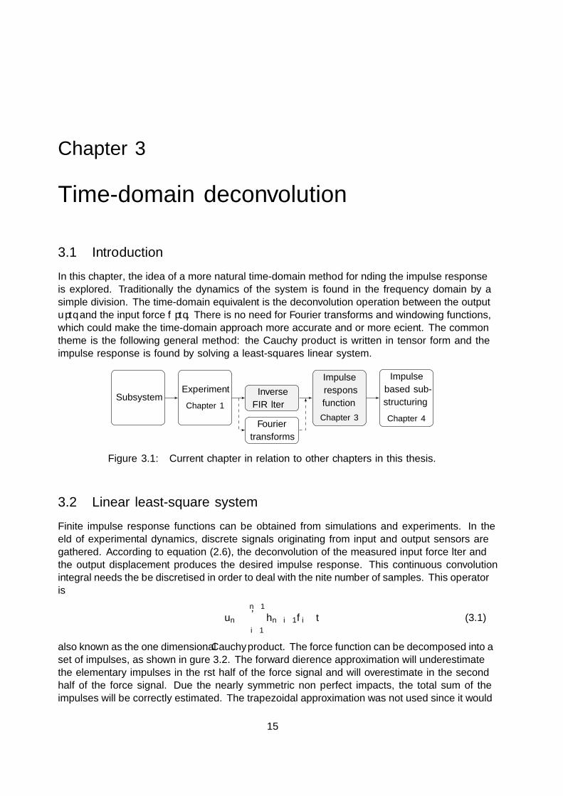
3.1 IntroductionIn this chapter, the idea of a more natural time-domain method for finding the impulse responseis explored. Traditionally the dynamics of the system is found in the frequency domain by asimple division. The time-domain equivalent is the deconvolution operation between the outputuptq and the input force fptq. There is no need for Fourier transforms and windowing functions,which could make the time-domain approach more accurate and or more efficient. The commontheme is the following general method: the Cauchy product is written in tensor form and theimpulse response is found by solving a least-squares linear system.
ExperimentChapter 1
Subsystem InverseFIR filter
Fouriertransforms
ImpulseresponsfunctionChapter 3
Impulsebased sub-structuringChapter 4
Figure 3.1: Current chapter in relation to other chapters in this thesis.
3.2 Linear least-square systemFinite impulse response functions can be obtained from simulations and experiments. In thefield of experimental dynamics, discrete signals originating from input and output sensors aregathered. According to equation (2.6), the deconvolution of the measured input force filter andthe output displacement produces the desired impulse response. This continuous convolutionintegral needs the be discretised in order to deal with the finite number of samples. This operatoris
un “n´1ÿ
i“1hn´i`1fi ∆t (3.1)
also known as the one dimensional Cauchy product. The force function can be decomposed into aset of impulses, as shown in figure 3.2. The forward difference approximation will underestimatethe elementary impulses in the first half of the force signal and will overestimate in the secondhalf of the force signal. Due the nearly symmetric non perfect impacts, the total sum of theimpulses will be correctly estimated. The trapezoidal approximation was not used since it would
15
16 3.2. Linear least-square system
introduce a delay in the response. The total response u at time t can be found by summing allthe responses due to the elementary impulses acting at all times τ .
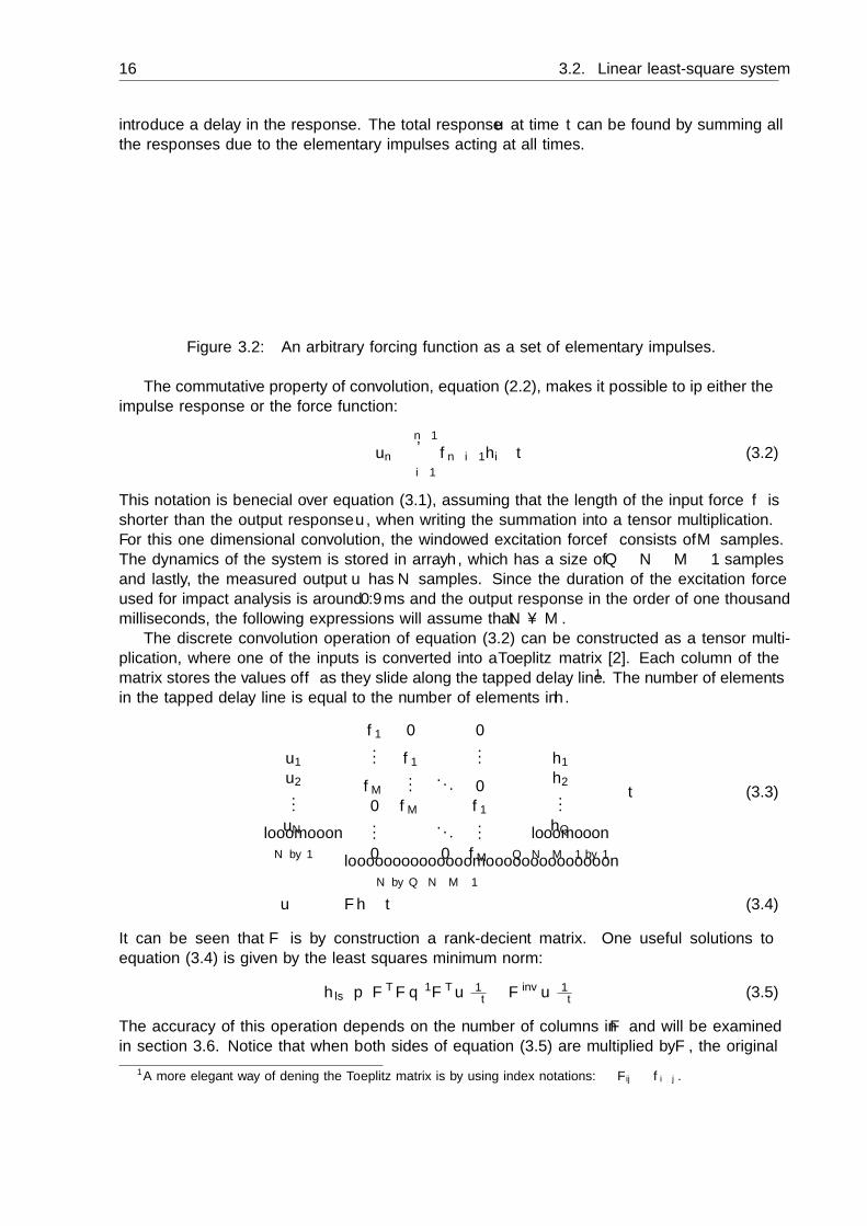
0 τ t
fpτq
∆τ
time [s]fo
rce
[N]
Figure 3.2: An arbitrary forcing function as a set of elementary impulses.
The commutative property of convolution, equation (2.2), makes it possible to flip either theimpulse response or the force function:
un “n´1ÿ
i“1fn´i`1hi ∆t (3.2)
This notation is beneficial over equation (3.1), assuming that the length of the input force f isshorter than the output response u, when writing the summation into a tensor multiplication.For this one dimensional convolution, the windowed excitation force f consists of M samples.The dynamics of the system is stored in array h, which has a size of Q “ N `M ´ 1 samplesand lastly, the measured output u has N samples. Since the duration of the excitation forceused for impact analysis is around 0.9ms and the output response in the order of one thousandmilliseconds, the following expressions will assume that N ěM .
The discrete convolution operation of equation (3.2) can be constructed as a tensor multi-plication, where one of the inputs is converted into a Toeplitz matrix [2]. Each column of thematrix stores the values of f as they slide along the tapped delay line1. The number of elementsin the tapped delay line is equal to the number of elements in h.
»
—
—
—
–
u1u2...uN
fi
ffi
ffi
ffi
fl
looomooon
N by 1
“
»
—
—
—
—
—
—
—
—
—
–
f1 0 ¨ ¨ ¨ 0... f1
...fM
... . . . 00 fM f1... . . . ...0 ¨ ¨ ¨ 0 fM
fi
ffi
ffi
ffi
ffi
ffi
ffi
ffi
ffi
ffi
fl
loooooooooooooomoooooooooooooon
N by Q“N´M`1
»
—
—
—
–
h1h2...hQ
fi
ffi
ffi
ffi
fl
looomooon
Q“N´M`1 by 1
∆t (3.3)
u “ Fh∆t (3.4)
It can be seen that F is by construction a rank-deficient matrix. One useful solutions toequation (3.4) is given by the least squares minimum norm:
hls “ pF TF q´1F Tu 1∆t “ F invu 1
∆t (3.5)
The accuracy of this operation depends on the number of columns in F and will be examinedin section 3.6. Notice that when both sides of equation (3.5) are multiplied by F , the original
1A more elegant way of defining the Toeplitz matrix is by using index notations: Fij “ fi´j .

Chapter 3. Time-domain deconvolution 17
equation (3.4) is obtained, since:
pF TF q´1F TF “ I (3.6)
The inverse filter matrix equivalent must thus be the pseudo inverse of the Toeplitz matrix
F inv “ pF TF q´1F T “ R´1F T (3.7)
The inverse FIR filter matrix of equation (3.7) is sufficient in solving the deconvolution operation,however the drawback is that the dimensions are prescribed by the output response lengthN . Take for example the measurement conducted in this thesis: N “ 32 768 and M “ 63.Finding the inverse of a very large matrix is costly and therefore this tensor multiplication isnot applicable for the field of experimental dynamics.
3.3 Inverse force filterInstead of a tensor multiplication, as presented in the previous section, a first order tensor isexplored that if convolved with the force filter, results in the unit impulse. This first ordertensor is the inverse of the force filter and will be called the inverse force filter f inv. It has tosatisfy the equation that holds for all inverses:
f ˙ f inv “ δ (3.8)
Because of the similarity with equation (3.6), the inverse filter F inv is the matrix counterpart ofthe inverse force filter vector f inv. The deconvolution operation can be performed by convolvingthe output u with the inverse filter f inv
h “ δ ˙ h “ f ˙ f inv ˙ h “ f inv ˙ u 1∆t (3.9)
The approximated impulse response h is the true impulse response if f inv is indeed the inversefilter to f , i.e. if equation (3.8) is satisfied. Formally, the inverse filter of a finite impulseresponse must be an infinite impulse response. Still it is possible to approximate a finite inverseforce filter that is shorter than N , resulting in a efficient impulse response estimation. Since thedeconvolution is performed using a convolution operation, the inverse filter length is no longerdependent on the length of the output response.
Now let us define the properties of the encountered matrices. If F is multiplied with anyarray, valid convolution is obtained. If F T is multiplied with any array, the linear correlation isfound. This is due to the fact that the transpose of the matrix eliminates the flip of the filter,which distinguishes the convolution from the correlation operation. So F TF “ R is equivalentto the linear auto-correlation of r “ f ‹ f . The correlation matrix R is examined for a filter fnwith n “ 1, 2, 3 and Q equal to five.
R “ F TF (3.10)
“
»
—
—
—
—
–
f1 f2 f3 0 0 0 00 f1 f2 f3 0 0 00 0 f1 f2 f3 0 00 0 0 f1 f2 f3 00 0 0 0 f1 f2 f3
fi
ffi
ffi
ffi
ffi
fl
»
—
—
—
—
—
—
—
—
–
f1 0 0 0 0f2 f1 0 0 0f3 f2 f1 0 00 f3 f2 f1 00 0 f3 f2 f10 0 0 f3 f20 0 0 0 f3
fi
ffi
ffi
ffi
ffi
ffi
ffi
ffi
ffi
fl
(3.11)

18 3.3. Inverse force filter
“
»
—
—
—
—
–
f21 ` f2
2 ` f23 f1f2 ` f2f3 f1f3 0 0
f1f2 ` f2f3 f21 ` f2
2 ` f23 f1f2 ` f2f3 f1f3 0
f1f3 f1f2 ` f2f3 f21 ` f2
2 ` f23 f1f2 ` f2f3 f1f3
0 f1f3 f1f2 ` f2f3 f21 ` f2
2 ` f23 f1f2 ` f2f3
0 0 f1f3 f1f2 ` f2f3 f21 ` f2
2 ` f23
fi
ffi
ffi
ffi
ffi
fl
(3.12)
“
»
—
—
—
—
–
r0 r´1 r´2 0 0r1 r0 r´1 r´2 0r2 r1 r0 r´1 r´20 r2 r1 r0 r´10 0 r2 r1 r0
fi
ffi
ffi
ffi
ffi
fl
(3.13)
It is observed that the full auto-correlation vector r is positioned in both the middle row andcolumn, see equation (3.13). This auto-correlation vector of an arbitrary filter will result in asymmetric signal. It is also seen that the correlation matrix R is symmetric and full rank andit’s inverse R´1 will therefore also be symmetric and full rank. Given the 35 components ofF , it is easy to compute the 15 components of R, but given R it is impossible to compute thecomponents of F .
Equation (3.8) will be essential in finding the inverse FIR filter. If the force in this con-volution operation is tranformed into a Toeplitz matrix, similar to that of equation (3.3), thefollowing form is found:
Ff inv “ δ (3.14)F TFf inv “ F Tδ (3.15)Rf inv “ F Tδ (3.16)f inv “ R´1F Tδ (3.17)
(3.18)
The expression F Tδ is equal to the reversed force vector, padded with Q´M zeros. The inverseFIR filter f inv is used in equation (3.9) to solve for the impulse response of a linear system.
3.3.1 Inverse FIR filter of non-perfect impact
A non-perfect impulse response created with an impact hammer is show in figure 3.3a. Thisbell shaped function clearly does not represents a unit impulse. The output response needsto be convolved with the inverse force filter to find the impulse response, as equation (3.9)prescribes. The inverse force filter to the non-perfect impact is shown in figure 3.3b and consistof Q samples.
In order to check the accuracy of the inverse force filter, the force function is convolved withthe inverse force filter. The output should result in the unit impulse, as shown in figure 3.3c.The theoretical value of the sum of all the values is one and will be used as the benchmark forthe accuracy of the inverse filter. The accuracy of the inverse force filter is determined by thenumber of columns Q in the Toeplitz matrix F and the conditioning of the correlation matrixR, which will be studied in section 3.6.
3.3.2 Impulse response reconstruction
The impulse response function is found by convolution of the output u with the inverse FIRfilter f inv, as shown in equation (3.9). The resulting sample length of h is due to the convolutionequal to N ` Q ´ 1. This is longer than the properties of convolution in section 2.2.1 define

Chapter 3. Time-domain deconvolution 19
1 d M0
200
400
600
samples [n]
f[N
]
(a) Non-perfect impact
1 Q´1
0
1 ¨10´2
samples [n]
fin
v[1
/N]
(b) Inverse force filter
1 i N
0
1
samples [n]
f˙
fin
v[-]
(c) Unit impulse with delay
Figure 3.3: The inverse FIR filter originated from a non-perfect impulse and the accuracycheck.
for the length of the impulse response. The sample length of the impulse response h should beequal to Q “ N ´M ` 1.
The impulse response is indeed present in the signal and only needs to be filtered out. Thereconstruction of the unit impulse f inv ˙ f “ δ is used in this process. The delay i at whichthe unit impulse is equal to one, as shown on the x-axis in figure 3.3c, is used to define the startpoint of the impulse response in h:
f inv ˙ f « δpn´ iq#
« 1 if i “ N`12
« 0 otherwise(3.19)
Now the impulse response can be reconstructed using the start point i and the theoretical samplelength of the impulse response Q. It is also found that the position d of the of the actual pulse inthe force window (figure 3.3a) is independent of the position of i. This is due to the symmetricauto correlation matrix.
3.4 Auto-correlation matrixThe auto-correlation of a noisy experimental imperfect impulse provides a better signal to noiseratio for detecting dominant frequency components compared to the original force function [6].In order to find the dominant frequencies in the auto-correlation vector, a Fourier transform isrequired:
rptq “ż 8
τ“´8fpτqfpt` τq dτ (3.20)
Frrptqs “ż 8
t“´8e´jωt
ˆż 8
τ“´8fpτqfpt` τq dτ
˙
dt (3.21)
“ż 8
τ“´8fpτq
ˆż 8
t“´8fpt` τqe´jωt dt
˙
dτ (3.22)
The Fourier transform of fpt` τq is F pωqejωτ . Therefore,
Frrptqs “ F pωqż 8
τ“´8fpτqejωτ dτ “ F pωqF p´ωq “ |F pωq|2 (3.23)
Equation (3.23) shows that the Fourier transform of the auto-correlation function is equal to theauto power spectral density. The auto-correlation matrix R is decomposed into it’s eigenvalues
20 3.4. Auto-correlation matrix
and eigenvectors to display the same information as the power spectral density in the timedomain. The eigenvalues represent the amount of energy and the corresponding eigenvectorsthe spectral distribution of this energy.
A perfect unit impulse will result in a dense set of frequencies. In order to accurately describethe impact response of a component, the selection criteria of the excitation signal is the powerdensity across the entire bandwidth. The energy density is found if matrix R is diagonalisedusing a sequence
λ1pRq ě ¨ ¨ ¨ ě λQpRq (3.24)
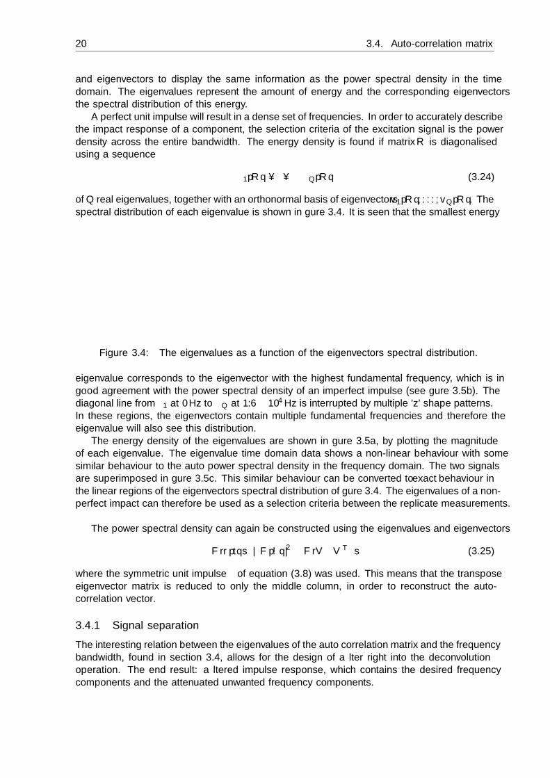
of Q real eigenvalues, together with an orthonormal basis of eigenvectors v1pRq, . . . ,vQpRq. Thespectral distribution of each eigenvalue is shown in figure 3.4. It is seen that the smallest energy
0 4000 8000 12000 16000λQ
λ1
frequency [Hz]
eige
nval
ue[-]
0
8 ¨ 10´4
dist
ribut
ion
[-]
Figure 3.4: The eigenvalues as a function of the eigenvectors spectral distribution.
eigenvalue corresponds to the eigenvector with the highest fundamental frequency, which is ingood agreement with the power spectral density of an imperfect impulse (see figure 3.5b). Thediagonal line from λ1 at 0Hz to λQ at 1.6ˆ 104 Hz is interrupted by multiple ’z’ shape patterns.In these regions, the eigenvectors contain multiple fundamental frequencies and therefore theeigenvalue will also see this distribution.
The energy density of the eigenvalues are shown in figure 3.5a, by plotting the magnitudeof each eigenvalue. The eigenvalue time domain data shows a non-linear behaviour with somesimilar behaviour to the auto power spectral density in the frequency domain. The two signalsare superimposed in figure 3.5c. This similar behaviour can be converted to exact behaviour inthe linear regions of the eigenvectors spectral distribution of figure 3.4. The eigenvalues of a non-perfect impact can therefore be used as a selection criteria between the replicate measurements.
The power spectral density can again be constructed using the eigenvalues and eigenvectors
Frrptqs “ |F pωq|2 “ FrV ΛV Tδs (3.25)
where the symmetric unit impulse δ of equation (3.8) was used. This means that the transposeeigenvector matrix is reduced to only the middle column, in order to reconstruct the auto-correlation vector.
3.4.1 Signal separation
The interesting relation between the eigenvalues of the auto correlation matrix and the frequencybandwidth, found in section 3.4, allows for the design of a filter right into the deconvolutionoperation. The end result: a filtered impulse response, which contains the desired frequencycomponents and the attenuated unwanted frequency components.

Chapter 3. Time-domain deconvolution 21
λ1 λQ
103
105
107
eigenvalue [-]
mag
nitu
de[N
2 ]
(a) Magnitude of the eigenvalues
0 4000 8000 12000 16000
10´6
10´4
10´2
frequency [Hz]
psd
[N2 /H
z]
(b) Auto power spectral density
(c) Superposition of the eigenvalues and theauto power spectral density
Figure 3.5: The magnitude of the eigenvalues and the power spectral density of a non-perfectimpact.
The shape of the auto power spectral density of the impact force shows that not all frequen-cies are excited with the same amount of energy. Consequently, there is a region of frequenciesthat receives a small amount of energy. In these regions, the output signal shows a increasedsignal to noise ratio. The deconvolution operation will strongly amplify the magnitude of thehigher frequencies to come to a constant energy level. This means that also the noise will beamplified. A filtered experimental impulse response is needed in the region where the energylevel is assumed to be constant. This in order to not amplify the uncertainties in the highfrequency region.
In order to find the impulse response in the region with assumed constant energy, the timedomain data is converted to the frequency domain, the signal is low-pass filtered and the filteredimpulse response is found after the inverse Fourier transform. A more direct approach can bepresented since the cutoff frequency fc of a low or high-pass filter can be linked to a singleeigenvalue λfc in the linear region of the eigenvectors spectral distribution (see figure 3.4).
Using the singular value decomposition the pseudo-inverse of the auto correlation matrixcan be easily computed as follows. Let R be decomposed into V ΛV T , then
R: “ V Λ:V T (3.26)
where the matrix Λ: takes the form:
Λ: “
»
—
—
—
–
1λ1
0 ¨ ¨ ¨ 00 1
λ2¨ ¨ ¨ 0
...... ¨ ¨ ¨ ...
0 0 ¨ ¨ ¨ 1λQ
fi
ffi
ffi
ffi
fl
(3.27)
for all of the non-zero singular values. If any of the λi are zero or assumed zero, then a zerois placed in corresponding entry of Λ:. If the amplitude of the eigenvalue corresponding to the

22 3.5. Time domain averaging
cutoff frequency is used as a tolerance for the pseudo inverse of the auto correlation matrix, theleast squares minimum norm is found for a filtered impulse response.
For a low-pass filter, all eigenvalues higher or equal to the eigenvalue of fs will be toleratedin the pseudo inverse. As an example, the non-perfect impact of figure 3.5 is considered and theinverse filter is defined using R:. The filtered and original impulse response and it’s spectralrepresentation are show in figure 3.6.
0 4 fc 8 12 16
10´1
101
frequency [kHz]
FR[m
/s2 /N
]
(a) Frequency response
0 2 4 6
´2
0
2
time [ms]
IR[m
/s2 /N
] original responsefiltered response
(b) Impulse response
Figure 3.6: The original and low-pass filtered frequency and impulse response. The cutofffrequency fc at the vertical gray line.
Figure 3.6a shows that the low frequency signals are passed and are a close match to theoriginal signal. It is also seen that the frequencies higher than the cutoff frequency are atten-uated. The filtered impulse response in figure 3.6b skips the high frequency oscillations in thefirst four milliseconds of the response. After this period a more smoothed signal is seen due tothe attenuated high frequency noise.
3.5 Time domain averagingAll experimental data is imperfect and the goals is to minimize errors. The systematic errorwill stay unknown, but the random error is minimized by doing several replicate measurementsand taking the average. In our case performing several impacts to the system and measuringthe output. The signal to noise ratio will be increased, theoretically in proportion to the squareroot of the number of measurements.
3.5.1 Response function estimators
The impulse response function estimator of equation (3.5) is given by the convolution of theinverse filter with the output response. The response function estimation in the frequencydomain is more well-known and is derived in a similar manner. The most common approach forthe estimation of frequency response functions is also by use of least squares techniques. Thealgorithms referred to as the H1 and H2 estimators are used based on the assumed locationof the noise entering the estimation process [1]. Next the H1 estimator will be given and thedirect link to the time domain inverse filter deconvolution:
H1pωq “ GfupωqGff pωq
DFTðñ hptq “ R´1ptqF T ptquptq (3.28)
The cross-power spectral density matrix Gfupωq is equal to F T ptquptq since the transpose ofthe Toeplitz matrix multiplied with any vector produces the linear cross correlation. The auto-power spectral density matrix Gff pωq of the force signal is stored in the time domain equivalent

Chapter 3. Time-domain deconvolution 23
auto correlation matrix R, as shown in section 3.4. This means that the impulse responsefunction estimation assumed that the location of noise is on the output response. By takingseveral replicate measurements and finding the average, the noise on the output is minimised.The H2 estimator and the coherence function will not be given since a time domain equivalentcan not directly be found in the deconvolution definition presented here.
3.5.2 Multiple input IRF estimation
The replicate measurements minimise the error on the output response and will be used in thetime domain averaging. Section 3.5.1 showed that the time domain deconvolution is equivalentto the H1 estimator, which for multiple inputs is defined as:
H1pωq “1{Navg
Navgř
i“1Gifupωq
1{Navg
Navgř
i“1Giff pωq
(3.29)
Note that one over the number of averages can be divided out of equation (3.29) and the crossand auto correlations needs to be calculated for every measurement.
The multiple input impulse response estimation suggested here will again make use of theToeplitz matrix, but will now be used for storing multiple force inputs F avg. The next examplegives the time domain averaging for two (i “ 1, 2) measurements
»
—
—
—
—
—
—
—
—
—
—
—
—
–
u1r1su1r2s...
u1rN su2r1su2r2s...
u2rN s
fi
ffi
ffi
ffi
ffi
ffi
ffi
ffi
ffi
ffi
ffi
ffi
ffi
fl
“
»
—
—
—
—
—
—
—
—
—
—
—
—
—
—
—
—
—
—
—
—
—
—
—
—
–
f1r1s 0 ¨ ¨ ¨ 0... f1r1s ...
f1rM s ... . . . 00 f1rM s f1r1s... . . . ...0 ¨ ¨ ¨ 0 f1rM s
f2r1s 0 ¨ ¨ ¨ 0... f2r1s ...
f2rM s ... . . . 00 f2rM s f2r1s... . . . ...0 ¨ ¨ ¨ 0 f2rM s
fi
ffi
ffi
ffi
ffi
ffi
ffi
ffi
ffi
ffi
ffi
ffi
ffi
ffi
ffi
ffi
ffi
ffi
ffi
ffi
ffi
ffi
ffi
ffi
ffi
fl
»
—
—
—
–
h1h2...
hN´M`1
fi
ffi
ffi
ffi
fl
∆t (3.30)
Again the least squares minimum norm will be used in finding the impulse response. The autocorrelation matrix for multiple input forces is defined as
Ravg “ F TavgF avg “
Navgÿ
i“1Ri (3.31)
The energy densities, as show in section 3.4, will be stores in the auto correlation vector butnow for the averaged impact. The conditioning of the averaged auto correlation matrix willdetermine the accuracy of the inverse filter and it’s therefore interesting to see how this numberis influenced by the sum of the auto correlation matrices.
24 3.6. Method validation
Eigenvalues The eigenvalues of the sum R1 `R2 of two Hermitian Q by Q matrices can bewritten in terms of the eigenvalues of R1 and R2. The eigenvalues are bounded by theinequalities [16]
λpR1 `R2qk`l´1 ď λpR1qk ` λpR2ql for k ` l ´ 1 ď Q (3.32)
The biggest eigenvalue of R1`R2 is bounded by one inequality: λpR1`R2q1 ď λpR1q1`λpR2q1, whereas the following sum of eigenvalues is bounded by an increasing amountof inequalities. Since the condition number depends on the first and last eigenvalue:λpR1`R2qQ ě λpR1qQ`λpR2qQ, the condition number decreases more beneficial than thelinear combination of the separate eigenvalues could suggest. This means that a replicatemeasurement with a large condition number can also be included into the averaging processwithout sacrificing on the accuracy.
The most costly operation is taking the inverse of the auto correlation matrix. In this averagingmethod, the inverse autocorrelation matrix is only calculated once and has the same size asthe auto correlation matrix of a single input force. Now the inverse filters are found when theinverse averaged auto correlation is correlated with the reversed single force pulses
f invi “ R´1avgF
Ti δ (3.33)
The impulse response reconstruction of multiple replicate measurements is estimated by thesummation of the inverse force filters convolved with the corresponding output responses ui
havg “Navgÿ
i“1f invi ˙ ui (3.34)
If the time domain IRF estimation of equation (3.34) is compared to the FRF estimator ofequation (3.29), it is seen that the factor 1{Navg is divided out of the equation in the spectralrepresentation and in the time domain this factor is found back in the inverse averaged autocorrelation vector. A difference between the two equations is that the auto correlation in thetime domain is only calculated once, whereas the spectral estimation needs to calculate the autocorrelation for every replicate measurement. The time-domain method is compared to that ofthe frequency domain estimator in figure A.1. A perfect match is found for both the amplitudeand phase.
3.6 Method validationThe accuracy and the computational time depend on two variables. In this section the sensitivityto these variables will be determined.
The Condition number of the auto-correlation matrix R is given by the ratio between thebiggest and lowest eigenvalue. The condition number for an unit impulse will be equalto one, which means that its inverse necessary for finding the inverse FIR filter can becomputed with good accuracy. If the condition number is large, then the matrix is said tobe ill-conditioned. Practically, such a matrix is almost singular, and the computation ofits inverse, or solution of a linear system of equations is prone to large numerical errors.A matrix that is not invertible has the condition number equal to infinity. An exampleto a non invertible auto-correlation matrix would be a sinusoidal force function of a singlefrequency.
Chapter 3. Time-domain deconvolution 25
The condition number of three experimentally obtain impulses is show in figure 3.7a as afunction of the output sample length. It is observed that the condition number reaches anupper bound, which means that the additional information in the autocorrelation matrixdoes not contribute to a more accurate calculation of the eigenvalues. If the replicatemeasurement with the lowest condition number is found in the accuracy plot of figure 3.7b,it is seen that a correlation matrix with the lowest condition number results in the inverseforce filter with the best accuracy.As shown in section 3.4, the eigenvalues represent the amount of energy and the eigenvectordetermines the distribution of the energy. If the point of observation is the frequencydomain, the ratio between the highest and lowest value of the auto power spectral densitywill give a good estimate for the condition number of R.
The accuracy of the inverse filter also depends on the dimensions of the Toeplitz matrix. Theaccuracy is defined as the absolute length of the samples that construct the unit impulse.Because the theoretical value should be equal to one, this number is also subtracted fromthis vale in order to graphically show the accuracy in figure 3.7b. The solid lines representthe accuracy check for time-domain acquired inverse force filters and the dashed linesrepresent the inverse filter found by frequency domain operations. The inverse filters inthe frequency domain are found by the following operation IDFTr1.{DFTrfptqss and isgraphically shown in figure 3.8.It is observed that the frequency domain gives an more accurate inverse filter. Thereare more calculations required for the time-domain approach, which gives more round offerrors, compared to that of the frequency domain method. For every force filter there willbe an optimum sample length N . The inverse filter will gradually get more accurate asthe output length increases and find an optimum between the region of lack of informationin the auto-correlation matrix and the region where the round-off errors are dominant.
The computational time is calculated as a function of the inverse filter length. Althoughspeed optimisations are not in the context of this thesis, for completeness the comparisonis made between the frequency and time-domain acquired inverse force filter. The resultsare shown in figure 3.7c. It is seen that the time-domain approach is at less time effi-cient (optimisations in the calculations, shown in appendix A.1, can lead to better timeefficiency).
3.7 SummaryTime-domain deconvolution is possible by defining an inverse FIR force filter which is indepen-dent of the output response. This inverse filter is convolved with the output response in order toobtain the impulse response function. The eigenvalue decomposition of the correlation matrixmakes choosing between replicate measurement and signal filtering possible. Averaging of mul-tiplicative measurements in time domain is possible and is equivalent to the frequency domainH1 estimator. The accuracy of the inverse filter is sensitive to the conditioning of the auto-correlation matrix and the inverse filter length. Due to more computations, the time-domainapproach is less accurate and less time efficient compared to that of the frequency domain ac-quired inverse filter. For a better understanding of the inverse force filter, a comparison is madebetween the two operational domains in figure 3.8.

26 3.7. Summary
102 103 104 105104
105
106
107
length f inv
cond
ition
ing
R[-]
(a) Conditioning of auto-correlation matrix R as afunction of the inverse filter length
102 103 104 10510´14
10´6
102
length f inv
|δ|´
1[-]
(b) The accuracy of the inverse FIR filter shown as afunction of the inverse filter length
102 103 104
100
102
length f inv
time
[ms]
(c) Computational time as a function of the inversefilter length
Figure 3.7: Sensitivity analysis on the accuracy of the time-domain inverse FIR filter (solidlines), for three experimentally obtained impacts. The dashed lines are inverseforce filters found through the frequency domain.

Chapter 3. Time-domain deconvolution 27
46 48 50 52 540
200400600
time [ms]
forc
e[N
]
(a) Input fptq and window
DFTðñ
0 8000 16000
10´2
100
frequency [Hz]fo
rce
[N]
(b) Input F pωq
88 89 90 91 92 93´1
´0.50
0.5¨10´2
time [ms]
fin
v[1
/N]
(c) Inverse force filter R´1F T δ
DFTðñ
0 8000 16000100
102
frequency [Hz]
fin
v[1
/N]
(d) Inverse force filter 1{F pωq
0 50 100 150 2000
0.5
1
time [ms]
δ[-]
(e) Unit impulse δptq
DFTðñ
0 8000 1600010´1
100
frequency [Hz]
δ[-]
(f) Unit impulse δpωq
Figure 3.8: Determination of the inverse force filter and the accuracy check in the time (left)and frequency domain (right).

Chapter 4
Dynamic substructuring usingimpulse response functions
4.1 Introduction
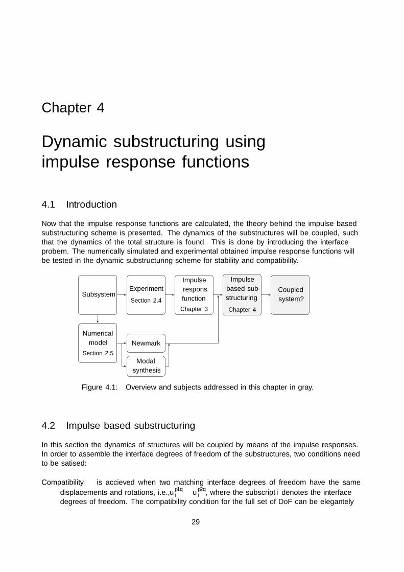
Now that the impulse response functions are calculated, the theory behind the impulse basedsubstructuring scheme is presented. The dynamics of the substructures will be coupled, suchthat the dynamics of the total structure is found. This is done by introducing the interfaceprobem. The numerically simulated and experimental obtained impulse response functions willbe tested in the dynamic substructuring scheme for stability and compatibility.
ImpulseresponsfunctionChapter 3
ExperimentSection 2.4
Subsystem
Numericalmodel
Section 2.5Newmark
Modalsynthesis
Impulsebased sub-structuringChapter 4
Coupledsystem?
Figure 4.1: Overview and subjects addressed in this chapter in gray.
4.2 Impulse based substructuring
In this section the dynamics of structures will be coupled by means of the impulse responses.In order to assemble the interface degrees of freedom of the substructures, two conditions needto be satisfied:
Compatibility is accieved when two matching interface degrees of freedom have the samedisplacements and rotations, i.e., up1qi “ up2qi , where the subscript i denotes the interfacedegrees of freedom. The compatibility condition for the full set of DoF can be elegantely
29

30 4.2. Impulse based substructuring
written using the signed Boolean matrix B, which selects the substructures interface DoF
Nsÿ
s“1Bpsqupsqn “ 0 (4.1)
Note that also compatibility can be claimed for the accelerations and velocities. In sec-tion 4.2.1, the interface DoF of the substructures are assumed to have the same velocity.
Equilibrium on the interface DoF is realised when the reaction forces are equal in magnitudeand opposite in sign: gp1q` gp2q “ 0. By making use of the same signed Boolean operatorfrom equation (4.1), this condition can be written as:
„
gp1qgp2q
“ ´BTλ, (4.2)
where λ are the unknown Lagrange multipliers that must be determined in order to satisfythe compatibility condition. So, the Lagrange multipliers represent the force necessary forkeeping the interface DoF connected.
4.2.1 Assembly of impulse responses
The velocity in time for a general applied force fptq can be found by approximating the convo-lution integral from equation (2.6) by the finite sum
9upsqn “nÿ
i“0
9Hn´i pf i ` giq∆t (4.3)
where the subscripts indicate the present time step: 9un “ 9uptnq. The sum running from i “ 0 ton states that 9H0 is non zero, this is also true for the accelerations :H0. When the displacementsare used for the impulse based substructuring, the impulse responseH0 on the first time step iszero and the summation limits can be shortened. The impulse response matrix for our systemwrites:
9Hn “«
9hp1q0 pnq 9hp1qL pnq9hp1qL pnq 9hp1q0 pnq
ff
(4.4)
Equation (4.3) is not consistent with the Newmark time integration scheme as shown in [12],since it assumes the force to be piecewise linear between tn and tn`1. If the impulse superpositionneeds to be consistent with the constant average acceleration Newmark, the impulse responsesare averaged and substituted in equation (4.3), as was proposed in [15]:
9Hn “ 1
2p 9Hn ` 9Hn`1q (4.5)
Substitution of the equilibrium and compatibility condition, respectively equations (4.1) and (4.2),into the impulse response in terms of velocities of equation (4.3), results in the coupled equations.
ˇ
ˇ
ˇ
ˇ
ˇ
ˇ
ˇ
ˇ
ˇ
ˇ
9upsqn “ ∆tnÿ
i“0
9Hpsqn´i pf psqi ´BpsqT λiq
Nsÿ
s“1Bpsq 9upsqn “ 0
(4.6)

Chapter 4. Dynamic substructuring using impulse response functions 31
The Lagrange multipliers λ represent the impulse needed for compatibility. By expanding thevelocities in time from equation (4.6), it can be quantified into two parts: a known part and anunderlined unknown part:
9upsqn “ ∆tn´1ÿ
i“0
9Hpsqn´i
´
fpsqi ´BpsqTλi
¯
`∆t 9Hpsq1 f psqn ´∆t 9
Hpsq1 BpsqT λn (4.7)
A prediction can be made from the known part in equation (4.7), called upsqn , of the substructuresvelocities when the interface forces gpsqn are equal to zero. The total velocities are thus writtenas
9upsqn “ 9upsqn ´∆t 9Hpsq1 BpsqT λn (4.8)
With this prediction on the velocities, the Lagrange multipliers needed to ensure compatibilityare calculated by substituting equation (4.8) in the compatibility condition of equation (4.6).
λn “˜
∆tNsÿ
s“1Bpsq 9Hpsq
1 BpsqT¸´1 Ns
ÿ
s“1Bpsq 9upsqn (4.9)
The term inside the braces needs to be inverted and can be seen as the effective dynamic stiffnesstensor for the interface degrees of freedom. The Lagrange multiplier is the magnitude of theforce necessary to keep the substructures together, i.e. the same internal force which is alwayspresent between discretised structural elements. Note that solving for the Lagrange multiplierson the interface is similar to the dual interface problem for the frequency based substructure[5]. Finally, a correction on the predicted velocity 9upsqn is made by solving equation (4.8). Thisprocedure is repeated for every time step.
4.3 Substructuring with numerical modelsThe full system is split up into two symmetric numerical models, as introduced in section 1.2.1.The impulse based substructuring scheme will try to ensure that the two substructures to-gether behave in the same way as the numerical full system. Next, the two ways of numericalsimulations, described in section 2.5, are tested for stability and compatibility.
4.3.1 Newmark time integration
The impulse response, found if the external excitation is equal to the unit impulse, is proven to beconsistent with the impulse based substructuring algorithm [12]. This means that the couplingprocess is independent of the time step. It will therefore be no surprise that the coupled responseis stable and compatibility ensures overlap of the full Newmark simulated response, as shown infigure 4.2a. The inherent periodicity error of the constant average acceleration scheme is equalfor the coupled and full simulated response.
4.3.2 Modal synthesis
The modally synthesised impulse response functions of the substructures, as presented in sec-tion 2.5.2, are not suitable for the coupling process. The result of the impulse based substruc-turing scheme with averaging shows a uncoupled stable response, see figure B.1b. From theimpulse response function of the substructures, in figure B.1a, it is observed that the magnitudeof the extremal values of the waves are underestimated.

32 4.3. Substructuring with numerical models
0
5
10
mob
ility
[m/s
/N]
IBS 9hpfullq2L
Newmark 9hpfullq2L
0
20
40m
obili
ty[m
/s/N
]IBS 9hpfullq
0
Newmark 9hpfullq0
0 2 4 6 8 10
0
0.2
time [ms]
lam
bda
[N]
(a) Coupling and reference Newmark IRF’s
´5
0
5
10
mob
ility
[m/s
/N]
IBS 9hpfullq2L
modal synthesis 9hpfullq2L
´20
0
20
40
mob
ility
[m/s
/N]
IBS 9hpfullq0
modal synthesis 9hpfullq0
0 2 4 6 8 10´2
0
2
4¨10´2
time [ms]
lam
bda
[N]
(b) Coupling and reference modally synthesised IRF’s
Figure 4.2: Impulse based substructuring using simulated impulse response functions.
The transient dynamic substructuring algorithm is proven to be consistent with the Newmarktime integration scheme. This implies that the inputs for the coupling process have to be equal tothe time integrated responses. This is only the case for time steps which approach zero: ∆tÑ 0,in which the Newmark time integrated response converges to the exact modally superimposedsolution. The convergence of the Newmark time integration to the analytical solution is sketchedin figure 4.3.
0 0.25 0.5´20
0
20
40
time [ms]
mob
ility
[m/s
/N] Newmark
modal synthesis
Figure 4.3: The convergence of Newmark (as a function of the step size) towards the analyticalsolution.

Chapter 4. Dynamic substructuring using impulse response functions 33
If the model is simulated with a time step which is ten times smaller as that of the experiment,the substructuring scheme produces a stable coupled impulse response, as shown in figure 4.2b.The coupled impulse responses are compared to that of the full model, with length equal to 2L.The results are in good agreement but come at a higher cost. The very small time step makesthe algorithm more computationally expensive. Due to the nature of the convolution product,the number of calculations grows quadratically with the number of samples.
4.4 Substructuring with experimental data
The experimentally obtained impulse response functions of the subcomponents are found withthe time-domain deconvolution operation, proposed in chapter 3, for 5 replicate measurementsand were shown in figure 2.7. The results of the impulse based substructuring scheme togetherwith the measurement of the full system are shown in figure 4.4.
´50
0
50
mob
ility
[m/s
/N]
9hpfullq2L IBS
9hpfullq2L measured
´50
0
50
mob
ility
[m/s
/N]
9hpfullq0 IBS
9hpfullq0 measured
0 tε 1 2 3 4 5´4´2
02
time [ms]
lam
bda
[N]
Figure 4.4: Impulse based substructuring using measured impulse response functions.
The end face 9hpfullq2L shows correct coupling up to the first period, which is at 0.6ms. The
rest of the signal is dominated by instability, which is assumed to start growing at tε; the firstwave of the cross point 9h
p1qL . At this instant in time, energy is gained into the system due to
increased amplitude of the impulse response compared to the first wave of the driving point 9hp1q0 .
Chapter 5 will give more detail to this reasoning, when its tried to alter the measured impulseresponse functions.

34 4.5. Summary
4.5 SummaryThe impulse response functions resulting from modal superposition will be a downsampledversion of the continuous underlying function, similar to that of the measurement. The Newmarktime integrated responses will converge to the analytical solution for very small time steps. Sincethe impulse based substructuring scheme is consistent with the Newmark time integration, onlymodally superimposed impulse response functions with high sampling rate can be used. Thiswill make the coupling process possible but at a higher cost.
The direct time-domain deconvolved, experimentally obtained, impulse response functionsdo not lead to a stable coupled system. The coupled results are dominated by instability, whichrenders them useless.

Chapter 5
Strategies for improvingexperimental IRF’s for dynamicsubstructuring
5.1 Introduction
The direct time domain deconvolution method did not change the impulse response function insuch an extend that dynamic substructuring was feasible, as was shown in section 4.4. Therefore,the flow chart in figure 5.1 does not give the operations necessary to get to the desired result:coupling experimental impulse response function. The problem of why the the coupling doesnot takes place is unknown and turns this part of the thesis into an exploratory research. Dueto the fundamental nature of this research, not all the possible options are investigated. Themost feasible options, in the effort of coupling experimental impulse response functions, arepresented in this chapter. The system was identified in chapter 2 both experimentally andnumerically, in order to spot the immediate difference between the two methods. Insight inthese differences gives rise to the formulation of hybrid impulse response functions. The perfectmodelled responses are also used to investigate operations which jeopardise the substructuringroutine, i.e. filtering, re-sampling and measurement errors. This chapter concludes with anoperation that gets rid of some experimental errors introduced into the impulse response.
SubsystemExperimentChapter 1
ImpulseresponsfunctionChapter 3
Impulsebased sub-structuringChapter 4
Coupledsystem:
No
Figure 5.1: The operations in flowchart do not lead to coupling of experimental impulse re-sponse functions.
5.2 Exploratory research
In contrast to the measured response, both simulated response functions could be successfullyused in the coupling process, as shown in chapter 4. In this section the apparent differences be-tween the two worlds of acquiring the impulse response are listed. These differences are labelledas possible problems why no coupling between measured responses takes place or instability
35
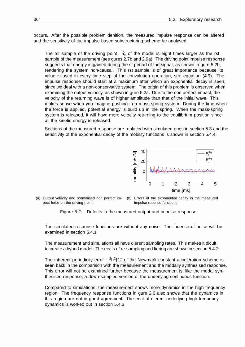
36 5.2. Exploratory research
occurs. After the possible problem definition, the measured impulse response can be alteredand the sensitivity of the impulse based substructuring scheme be analysed.
• The first sample of the driving point 9h10 of the model is eight times larger as the first
sample of the measurement (see figures 2.7b and 2.9a). The driving point impulse responsesuggests that energy is gained during the fist period of the signal, as shown in figure 5.2b,rendering the system non-causal. This first sample is of great importance because itsvalue is used in every time step of the convolution operation, see equation (4.9). Theimpulse response should start at a maximum after which an exponential decay is seen,since we deal with a non-conservative system. The origin of this problem is observed whenexamining the output velocity, as shown in figure 5.2a. Due to the non perfect impact, thevelocity of the returning wave is of higher amplitude than that of the initial wave. Thismakes sense when you imagine pushing in a mass-spring system. During the time whenthe force is applied, potential energy is build up in the spring. When the mass-springsystem is released, it will have more velocity returning to the equilibrium position sinceall the kinetic energy is released.
Sections of the measured response are replaced with simulated ones in section 5.3 and thesensitivity of the exponential decay of the mobility functions is shown in section 5.4.4.
20 21 22 230
0.5
1
time [ms]
outp
utve
loci
ty[m
/s]
9up1q0
force
(a) Output velocity and normalised non perfect im-pact force on the driving point
0 1 2 3 4 5
0
20
40
time [ms]
mob
ility
[m/s/N
]
9hp1q0
9hp1qL
(b) Errors of the exponential decay in the measuredimpulse resonse functions
Figure 5.2: Defects in the measured output and impulse response.
• The simulated response functions are without any noise. The influence of noise will beexamined in section 5.4.1
• The measurement and simulations all have different sampling rates. This makes it difficultto create a hybrid model. The effects of re-sampling and filtering are shown in section 5.4.2.
• The inherent periodicity error ω2h2{12 of the Newmark constant acceleration scheme isseen back in the comparison with the measurement and the modally synthesised response.This error will not be examined further because the measurement is, like the modal syn-thesised response, a down-sampled version of the underlying continuous function.
• Compared to simulations, the measurement shows more dynamics in the high frequencyregion. The frequency response functions in figure 2.6 also shows that the dynamics inthis region are not in good agreement. The effect of different underlying high frequencydynamics is worked out in section 5.4.3
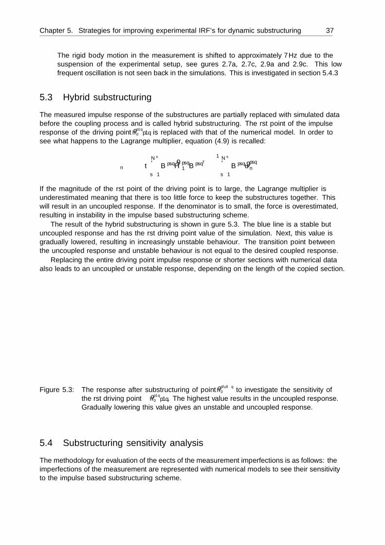
Chapter 5. Strategies for improving experimental IRF’s for dynamic substructuring 37
• The rigid body motion in the measurement is shifted to approximately 7Hz due to thesuspension of the experimental setup, see figures 2.7a, 2.7c, 2.9a and 2.9c. This lowfrequent oscillation is not seen back in the simulations. This is investigated in section 5.4.3
5.3 Hybrid substructuring
The measured impulse response of the substructures are partially replaced with simulated databefore the coupling process and is called hybrid substructuring. The first point of the impulseresponse of the driving point 9h
p1q0 p1q is replaced with that of the numerical model. In order to
see what happens to the Lagrange multiplier, equation (4.9) is recalled:
λn “˜
∆tNsÿ
s“1Bpsq 9Hpsq
1 BpsqT¸´1 Ns
ÿ
s“1Bpsq 9upsqn
If the magnitude of the first point of the driving point is to large, the Lagrange multiplier isunderestimated meaning that there is too little force to keep the substructures together. Thiswill result in an uncoupled response. If the denominator is to small, the force is overestimated,resulting in instability in the impulse based substructuring scheme.
The result of the hybrid substructuring is shown in figure 5.3. The blue line is a stable butuncoupled response and has the first driving point value of the simulation. Next, this value isgradually lowered, resulting in increasingly unstable behaviour. The transition point betweenthe uncoupled response and unstable behaviour is not equal to the desired coupled response.
Replacing the entire driving point impulse response or shorter sections with numerical dataalso leads to an uncoupled or unstable response, depending on the length of the copied section.
0 0.5 1 1.5 2 2.5 3´50
0
50
time [ms]
mob
ility
[m/s
/N] high
low
Figure 5.3: The response after substructuring of point 9hpfullq0 to investigate the sensitivity of
the first driving point 9hp1q0 p1q. The highest value results in the uncoupled response.
Gradually lowering this value gives an unstable and uncoupled response.
5.4 Substructuring sensitivity analysis
The methodology for evaluation of the effects of the measurement imperfections is as follows: theimperfections of the measurement are represented with numerical models to see their sensitivityto the impulse based substructuring scheme.
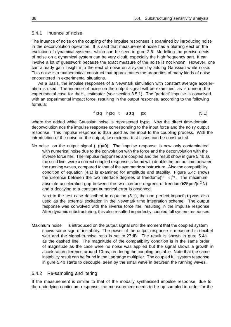
38 5.4. Substructuring sensitivity analysis
5.4.1 Influence of noise
The influence of noise on the coupling of the impulse responses is examined by introducing noisein the deconvolution operation. It is said that measurement noise has a blurring effect on theevolution of dynamical systems, which can be seen in figure 2.6. Modelling the precise effectsof noise on a dynamical system can be very difficult, especially the high frequency part. It caninvolve a lot of guesswork because the exact measure of the noise is not known. However, onecan already gain insight into the effect of noise on a system by adding Gaussian white noise.This noise is a mathematical construct that approximates the properties of many kinds of noiseencountered in experimental situations.
As a basis, the impulse responses of a Newmark simulation with constant average acceler-ation is used. The influence of noise on the output signal will be examined, as is done in theexperimental case for the H1 estimator (see section 3.5.1). The ’perfect’ impulse is convolvedwith an experimental impact force, resulting in the output response, according to the followingformula:
fptq˙ hptq∆t “ uptq ` ζptq (5.1)
where the added white Gaussian noise is represented by ζptq. Now the direct time-domaindeconvolution finds the impulse response corresponding to the input force and the noisy outputresponse. This impulse response is than used as the input to the coupling process. With theintroduction of the noise on the output, two extrema test cases can be constructed:
No noise on the output signal (ζ(t)=0). The impulse response is now only contaminatedwith numerical noise due to the convolution with the force and the deconvolution with theinverse force filter. The impulse responses are coupled and the result show in figure 5.4b asthe solid line, were a correct coupled response is found with double the period time betweenthe running waves, compared to that of the symmetric substructure. Also the compatibilitycondition of equation (4.1) is examined for amplitude and stability. Figure 5.4c showsthe difference between the two interface degrees of freedom
ˇ
ˇ
ˇ:up1qL ´ :u
p2q0
ˇ
ˇ
ˇ. The maximum
absolute acceleration gap between the two interface degrees of freedom is 0.25pm/(s2 N)and a decaying to a constant numerical error is observed.Next to the test case described in equation (5.1), the non perfect impact fptq was alsoused as the external excitation in the Newmark time integration scheme. The outputresponse was convolved with the inverse force filter, resulting in the impulse response.After dynamic substructuring, this also resulted in perfectly coupled full system responses.
Maximum noise is introduced on the output signal until the moment that the coupled systemshows some sign of instability. The power of the output response is measured in decibelwatt and the signal-to-noise ratio is set to 27dB. The result is shown in figure 5.4aas the dashed line. The magnitude of the compatibility condition is in the same orderof magnitude as the case were no noise was applied but the signal shows a growth inacceleration difference around 10ms, rendering the coupling unstable. Note that the sameinstability result can be found in the Lagrange multiplier. The coupled full system responsein figure 5.4b starts to decouple, seen by the small wave in between the running waves.
5.4.2 Re-sampling and filtering
If the measurement is similar to that of the modally synthesised impulse response, due tothe underlying continuum response, the measurement needs to be up-sampled in order for the
Chapter 5. Strategies for improving experimental IRF’s for dynamic substructuring 39
0 5
0
2
4
time [ms]
IR[m
{s2 {N] ζ “ 27 dB
reference
(a) Impulse response :hp1qL of sub-
structure. The solid line thenoise due to deconvolution andthe dashed line the added whiteGaussian noise.
0 5
0
2
time [ms]
IR[m
{s2 {N]
(b) Impulse response :hpfullq2L of full
model after impulse based sub-structuring.
0 5 10 15 200
1
time [ms]
gap
[pm
/(s2
N)]
(c) The absolute acceleration differ-ence between the interface de-grees of freedom.
Figure 5.4: The input, output and the gap between the substructures of the dynamic sub-structuring process when noise is added.
impulse based substructuring scheme to work. It is possible for the modal superimposed resultof the substructures to be re-sampled before acquiring the coupled response. The same attempton the measurement failed due to the inclusion of measurement noise on the signal.
A possibility for finding cleaner impulse response functions is by applying a low pass filter.This will get rid of the high frequency noise and mismatching dynamics. There are again twoways of filtering the system, a time-domain approach as proposed in section 3.4.1 and in thefrequency main with a Butterworth filter [3]. The filtering process was tested on simulatedresponses. Dynamic substructuring after the responses of the substructures were filtered ledto instability in the results. The filtering process has a big influence on the first point of thedriving point, such that no fluent exponential decay is spotted in the impulse response functionsof the substructures.
5.4.3 Change underlying dynamics
In order to see the influence of the mismatching high frequency dynamics, as was seen for themeasured substructures (figure 2.6), a numerical model will be tuned. The modal parametersof the perfect simulation are altered to give a different impulse response for one of the interfacedegrees of freedom. The cross point 9h
p1qL is the modelled response and the driving point 9h
p1q0 is
altered. The high frequency response, after 9 kHz, now contains different eigenfrequencies anddamping parameters. The frequency response function is shown in figure 5.6a, where the dottedblack line is changed into the red dashed line. The effects in the transient response is shown infigure 5.5a. It clearly shows different high frequency dynamics in the beginning of the signal aslong as the damping ratio allows.
The substructures with mismatching underlying dynamics are now tested in the impulsebased substructuring scheme. The result is presented in figure 5.5b. The substructured responsedoes not show perfect coupling during the first period of the signal (the red dashed line). Theintroduced error has however no influence on the remaining response. This is remarkable, sincethe Lagrange multipliers ensuring compatibility in the first period are also used in the proceedingcalculations of the convolution operation. The error is not big enough for creating an immediateunstable behaviour. As the error is quickly damped out, due to the high frequency dampingratio, also does the error on the Lagrange multiplier.

40 5.4. Substructuring sensitivity analysis
0 1 2 3´20
0
20
40
time [ms]
mob
ility
[m/s
/N]
9hp1q0 modified
9hp1q0
(a) Changed high frequency of subcomponsent
0 1 2 3 4 5´20
0
20
40
time [ms]
mob
ility
[m/s
/N]
9hpfullq0 IBS modified
9hpfullq0 IBS
(b) IBS of perfect and coupled response with changedhigh frequency dynamics of driving point subcom-ponent
Figure 5.5: Only the high frequency characteristics of the driving point are altered, after whichthe impulse based substructuring scheme is conducted.
0 4000 8000 12000 16000101
102
103
104
frequency [Hz]
mob
ility
[m/s
/N]
9hp1q0 9hp1q
L9hp1q
0 modified
(a) Changed high frequency dynamics
0 4000 8000 12000 16000101
102
103
frequency [Hz]
mob
ility
[m/s
/N]
9hp1q0
9hp1q0 ` ε
(b) Amplitude error
Figure 5.6: Frequency response functions of the driving point where first the dynamics andlater the amplitude is changed.
The same procedure was also followed by shifting the rigid body mode to a higher frequency,but mismatching for the two interface degrees of freedom. Again a stable and coupled responsewas observed.
5.4.4 Exponential decay
The simulated data shows constant exponential delay in the impulse response functions. Fig-ure 5.2b shows that this is not at all the case for the measurement. No exponential functioncan be plotted through the peak of the waves. Four obvious points are picked at time p1 to p4in this figure. The non perfect impact is the cause for the amplitude error of peak p1. Mea-surement induced errors such as small differences in the frequency of the rigid body mode anddiscretisation error can be the cause for the amplitude error of peak p3.
This problem is again simulated using numerical data. At time tε an error is introducedinto the impulse response function. The simulation is shown in figure 5.7a, where the dottedblack line is the perfect response and the solid blue line containing the small amplitude error.The error in this example is ε “ 5%, but the same behaviour also occurs for an error of lessthan one percent. The impulse response functions are now coupled and shown in figure 5.7b.An amplitude error on the second (or any) period will decouple the subsystems. If the change
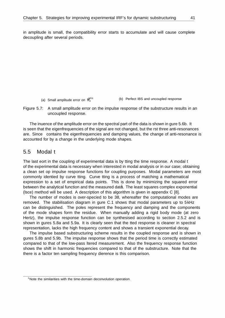
Chapter 5. Strategies for improving experimental IRF’s for dynamic substructuring 41
in amplitude is small, the compatibility error starts to accumulate and will cause completedecoupling after several periods.
0.2 0.4 tε 0.8 1
0
10
time [ms]
mob
ilibt
y[m
/s/N
]
9hp1q0 9hp1q
L9hp1q
0 ` ε
(a) Small amplitude error on 9hp1q0
0 tε 1 2 3 4 5´5
0
5
10
time [ms]
mob
ility
[m/s
/N]
9hpfullq0
9hpfullq0 ` ε
(b) Perfect IBS and uncoupled response
Figure 5.7: A small amplitude error on the impulse response of the substructure results in anuncoupled response.
The influence of the amplitude error on the spectral part of the data is shown in figure 5.6b. Itis seen that the eigenfrequencies of the signal are not changed, but the first three anti-resonancesare. Since λ contains the eigenfrequencies and damping values, the change of anti-resonance isaccounted for by a change in the underlying mode shapes.
5.5 Modal fitThe last effort in the coupling of experimental data is by fitting the time response. A modal fitof the experimental data is necessary when interested in modal analysis or in our case; obtaininga clean set op impulse response functions for coupling purposes. Modal parameters are mostcommonly identified by curve fitting. Curve fitting is a process of matching a mathematicalexpression to a set of empirical data points. This is done by minimizing the squared errorbetween the analytical function and the measured data1. The least squares complex exponential(lsce) method will be used. A description of this algorithm is given in appendix C [8].
The number of modes is over-specified to be 38, whereafter the computational modes areremoved. The stabilisation diagram in figure C.1 shows that modal parameters up to 5 kHzcan be distinguished. The poles represent the frequency and damping and the componentsof the mode shapes form the residue. When manually adding a rigid body mode (at zeroHertz), the impulse response function can be synthesised according to section 2.5.2 and isshown in figures 5.8a and 5.9a. It is clearly seen that the fitted response is cleaner in spectralrepresentation, lacks the high frequency content and shows a transient exponential decay.
The impulse based substructuring scheme results in the coupled response and is shown infigures 5.8b and 5.9b. The impulse response shows that the period time is correctly estimatedcompared to that of the low-pass filtered measurement. Also the frequency response functionshows the shift in harmonic frequencies compared to that of the substructure. Note that thethere is a factor ten sampling frequency difference is this comparison.
1Note the similarities with the time-domain deconvolution operation.

42 5.5. Modal fit
0 4000 8000 12000 16000100
101
102
103
frequency [Hz]
mob
ility
[m/s
/N]
measurementlsce
(a) Measurement and lsce fit of subsystem
0 4000 8000 12000 16000100
101
102
103
frequency [Hz]
mob
ility
[m/s
/N]
measurement9hpfullq
0 IBS
(b) Measurement and IBS response of length 2L
Figure 5.8: FRF’s of measurement, lsce fit and IBS coupled response.
0
5
10
15
mob
ility
[m/s
/N]
9hp1q0 lsce
9hp1q0 measurement
0 1 2 3 4 5
0
5
10
15
time [ms]
mob
ility
[m/s
/N]
9hp1qL lsce
9hp1qL measurement
(a) Modal fit of subsystem
0
5
10
mob
ility
[m/s
/N]
9hpfullq2L IBS
9hpfullq2L measurement
0
5
10
15
mob
ility
[m/s
/N]
9hpfullq0 IBS
9hpfullq0 measurement
0 1 2 3 4 5
´2
0
2¨10´2
time [ms]
lam
bda
[N]
(b) Coupled full system responses
Figure 5.9: Modal fit of subsystems and the IBS coupled responses.
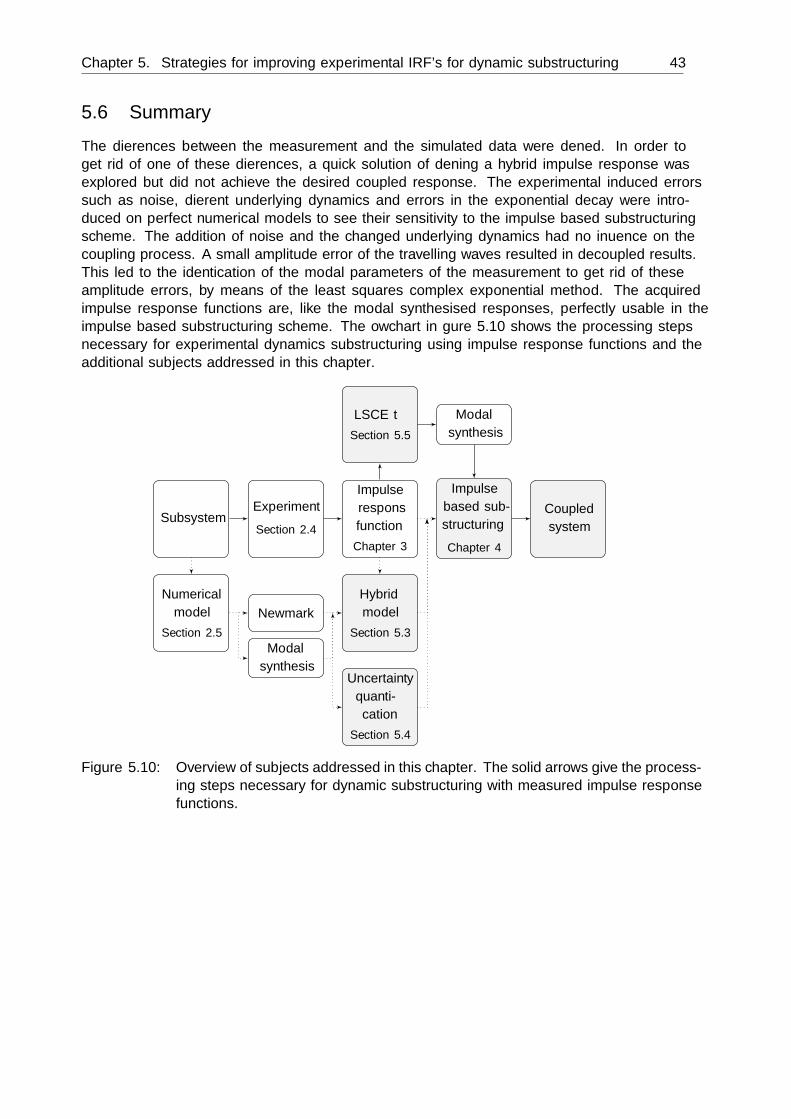
Chapter 5. Strategies for improving experimental IRF’s for dynamic substructuring 43
5.6 SummaryThe differences between the measurement and the simulated data were defined. In order toget rid of one of these differences, a quick solution of defining a hybrid impulse response wasexplored but did not achieve the desired coupled response. The experimental induced errorssuch as noise, different underlying dynamics and errors in the exponential decay were intro-duced on perfect numerical models to see their sensitivity to the impulse based substructuringscheme. The addition of noise and the changed underlying dynamics had no influence on thecoupling process. A small amplitude error of the travelling waves resulted in decoupled results.This led to the identification of the modal parameters of the measurement to get rid of theseamplitude errors, by means of the least squares complex exponential method. The acquiredimpulse response functions are, like the modal synthesised responses, perfectly usable in theimpulse based substructuring scheme. The flowchart in figure 5.10 shows the processing stepsnecessary for experimental dynamics substructuring using impulse response functions and theadditional subjects addressed in this chapter.
ImpulseresponsfunctionChapter 3
ExperimentSection 2.4
Subsystem
Numericalmodel
Section 2.5
LSCE fitSection 5.5
Newmark
Modalsynthesis
Impulsebased sub-structuringChapter 4
Hybridmodel
Section 5.3
Coupledsystem
Modalsynthesis
Uncertaintyquantifi-cation
Section 5.4
Figure 5.10: Overview of subjects addressed in this chapter. The solid arrows give the process-ing steps necessary for dynamic substructuring with measured impulse responsefunctions.

Chapter 6
Conclusions and recommendations
6.1 Conclusions
In this work, a direct time-domain deconvolution operation has been developed and tested.This method is based on writing the Cauchy product in tensor form and the impulse response isfound by solving a least-squares linear system. The formulation of the inverse FIR force filter,which is independent of the output response, allows for averaging between measurements and ahigh, low or bandpass filter can be built into the deconvolution operation. The latter is done bymaking use of the eigenvalues of the auto correlation matrix and formulating a pseudo inverse(section 3.4). The magnitude of the eigenvalues are similar to the auto power spectral densityand can thus be used as a selection criteria between replicate measurements. The definitionof the inverse filter is tested on three non perfect impacts to gain insight in its performance(section 3.6). It was found that the size of the Toeplitz matrix and the conditioning of the autocorrelation matrix defines the accuracy and computational cost of the inverse filter. The inversefilter can also be defined by using a Fourier transform and its inverse. If both methods arecompared, it is shown that the time-domain approach is less accurate and time efficient.
The equations of motion are solved by a Newmark time integration scheme and a modal syn-thesis. It was shown that the velocity can best be used for experimental dynamic substructuringpurposes (section 2.5). The velocity is a superposition of delayed cosine functions and is lesssensitive to trigger issues compared to the superposition of sine functions of the displacementand acceleration around t “ 0. Another reason for abandoning the acceleration is the negativeanalytical value at time equal to zero, which leads to direct instability in the impulse basedsubstructuring scheme.
The time integrated response functions can be used in the impulse based substructuringscheme independent of the size of the time step. The modally synthesised impulse responsefunction can only be used for dynamic substructuring if the time steps are very small. TheNewmark time integration scheme, which is consistent with the substructuring scheme, con-verges to the analytical solution for these small time steps. This makes coupling of modalsynthesised impulse response functions very computationally demanding. The close correspon-dence of the measurement and the analytical solution, which are both down-sampled versions ofthe underlying continuum response, implies that the experimental data also needs a time stepthat is very small (section 4.3).
The direct time-domain deconvolution did not change the impulse response in such an extendthat impulse based substructuring was possible (section 4.4). The observation of the differencesbetween the measured and simulated data resulted in several test cases. A hybrid impulseresponse was constructed, sections of the measurement are replaced with simulated data, but did
45
46 6.2. Recommendations
not lead to a coupled stable response. The impulse based substructuring scheme is not sensitiveto change of noise level, change in underlying dynamics and up-sampling of the analyticalresponse. Note that this does not imply that a combination of these factors lead to a stablecoupled response. The scheme is very sensitive to amplitude errors on the travelling waves. Anamplitude error, a change in the exponential decay, less than one percent lead to decoupled fullsystem responses (section 5.4.4).
The modal parameters of the measured impulse response functions are obtained by using theleast squares complex exponential method, which operated in the time-domain. These modalparameters were utilised in synthesising a clean impulse response with a perfect exponentialdecay. The clean impulse response functions as the input for the impulse based substructuringscheme resulted in successful coupling (section 5.5).
6.2 RecommendationsDue to the fundamental nature of the exploratory research, not all the possible changes to thetime measured impulse response were investigated in the effort of finding a coupled experimentalresponse. Chapters 4 and 5 showed that dynamic substructuring with raw and slightly changedexperimental impulse response functions was not possible. Fitting a pole-residue model on theempirical data made dynamic substructuring possible. The modal fit is a costly procedure andwould ideally be avoided. The peaks of the travelling waves of the measurement could be scaledto a numerically obtained exponential decay, such the energy in the system is gradually reduced.Another change to the impulse response without fitting a model would be to compensate forthe error in the output response, due to the non perfect impact, by the law of conservation ofenergy.
If the modal fit of the measured data stays necessary, the impulse based substructuringscheme is too expensive for the calculation of long time responses. Since it uses modal synthesisedimpulse response functions, the time step needs to approach zero to be consistent with thesubstructuring scheme. A substructuring scheme that is independent of the time step for modalsynthesised response functions is very welcome.
6.2.1 Outlook
Next, the possibilities of the inverse filter will be discussed. Using the inverse filter is attractivewhen either the input or impulse response is known on forehand and the deconvolution operationneeds to be performed in real-time. Another application would be to avoid the frequency domaineffect of leakage.
Lightly damped structures are costly to test experimentally. The long vibration time makestesting and data storage expensive. The system must be completely damped out to obtainthe most accurate frequency and damping parameters and avoid the frequency domaineffect of leakage. The inverse force filter could change this procedure by deconvolvingonly the first part of the output response. Since the inverse filter is independent of theoutput response and operates in the time-domain, spectral leakage has no influence on theobtained impulse response. The truncation error, made by only taking a small section ofthe output response, is shown in figure D.1. A modal fit can be used on a short sectionof the impulse response for finding correct amplitude and phase parameters. These modalparameters are used for synthesising the complete impulse response.
The impulse response is known either from experimental testing or numerical modelling.This means that the inverse impulse response can be computed on forehand. If the output

Chapter 6. Conclusions and recommendations 47
response is measured in real-time, the inverse filter allows for obtaining the input responsewith a theoretical delay of the time step ∆t. The truncation error of only using the firstfew periods is small, as graphically shown in figure D.1. This is done to keep the inversefilter of reasonable length.A possible example for this application would be in the railway industry, where there isa need for the determination of different imperfections on the track. These imperfectionsintroduce impact forces on the steel wheels of the train during motion. If the outputresponse is measured in the bearings, the inverse impulse response could determine theimpact force, if the system is assumed to behave linearly, in real time. With the knownimpact force, different imperfections can be quantified by examining the magnitude of itseigenvalues, i.e. the spectral content of the impact.
The input force is known in advance with a specific degree of certainty. The deconvolutionoperation, using the inverse filter, allows for the determination of the impulse response ata delay of the time step. The point wise availability of the impulse response can be usedin the impulse based substructuring scheme, such that coupling in real time is possible (ifthe time step approaches zero).

Bibliography
[1] J.S. Bendat and A.G. Piersol. Engineering applications of correlation and spectral analysis.J. Wiley, 1993.
[2] M Bertero and P Boccacci. Introduction to inverse problems in imaging. Bristol, Philadel-phia, 1998.
[3] S Butterworth. On the Theory of Filter Amplifiers. Wireless Engineer, 7, 1930.
[4] WH Kautz. Transient synthesis in the time domain. Circuit Theory, Transactions of theIRE Professional Group on, (3):29–39, 1954.
[5] D de Klerk, DJ Rixen, and SN Voormeeren. General framework for dynamic substructuring:history, review and classification of techniques. AIAA journal, 46(5):1169–1181, 2008.
[6] YW Lee, TP Cheatham Jr, and JB Wiesner. Application of correlation analysis to thedetection of periodic signals in noise. Proceedings of the IRE, 38(10):1165–1171, 1950.
[7] L Lehmann. An effective finite element approach for soil-structure analysis in the time-domain. Structural Engineering and Mechanics, 21(4):437–450, 2005.
[8] N.M.M. Maia and J.M.M. Silva. Theoretical and Experimental Modal Analysis. Engineeringdynamics series. Research Studies Press Limited, 1997.
[9] N.M. Newmark. A method of computation for structural dynamics. Journal of the Engi-neering Mechanics Division of ASCE 85, pages 67–94, 1959.
[10] Daniel J Rixen. A substructuring technique based on measured and computed impulseresponse functions of components. ISMA, 2010.
[11] Daniel J Rixen. Substructuring using impulse response functions for impact analysis. InStructural Dynamics, Volume 3, pages 637–646. Springer, 2011.
[12] Daniel J. Rixen and Paul L.C. van der Valk. An impulse based substructuring approach forimpact analysis and load case simulations. Journal of Sound and Vibration, 332(26):7174– 7190, 2013.
[13] P.L.C. Valk and D.J. Rixen. An Effective Method for Assembling Impulse Response Func-tions to Linear and Non-Linear Finite Element Models. In Topics in Experimental Dynam-ics Substructuring and Wind Turbine Dynamics, Volume 2, Conference Proceedings of theSociety for Experimental Mechanics Series, pages 123–135. Springer New York, 2012.
[14] T. van der Horst and F. Wenneker. Experimental dynamic analysis on a high-end Aristidesguitar. Technical report, Delft Unversity of Technology, special project: ME1460, May2012.
49

50 Bibliography
[15] Maarten M.V. van der Seijs and Daniel J. Rixen. Efficient impulse based substructuringusing truncated impulse response functions and mode superpositon. Proceedings of ISMA2012, 2012.
[16] H. Wielandt. An extremum property of sums of eigenvalues. Proceedings of the AmericanMathematical Society, 6:106–110, 1955.

Appendix A
Inverse force filter
A.1 Implementation
1 function[h,time] = irf(f,u,N,dt)2 % irf Performes the deconvolution between the input f and output3 % u resulting in the impulse response h, for single4 % or multiple measurements.5 % [f] Interval of the force function of interest, column matrix6 % [f1;f2;..] (windowed with lower and upper bound), M an odd number.7 % [u] Output u starts at the lower bound of the force window,column8 % matrix [u1;u2,..].9 % [N] An odd number specifying the accuracy of the inverse filter, scale
10 % approx 4001 (depending on theconditioning of R).11 % [dt] Samping rate.12 %13
14 [M,b] = size(f);15 Q = N M+1;16 U = numel(u(:,1));17 % Correlation matrix18 S = 2*M´1; % length auto correlation vector19 r = zeros(1,S);20
21 for j = 1:b22 r = r + xcorr(f(:,j)).'; % (sum) auto correlation vector23 end24
25 % Auto correlation matrix26 R = sparse(N+M´1,Q);27
28 for i=1:Q,29 R(i:((S+i´1)),i) = r;30 end31 O = (N+M´1 Q)/2;32 R = R(O+1:N+M´1 O,:);33
34 % Inverse force filter and convolution35 f_inv = zeros(Q,b);36 hhat = zeros(U+Q´1,b);37 for j= 1:b38 frv = [zeros((Q M)/2,1); flipud(f(:,j));zeros((Q M)/2,1)];39 f_inv(:,j) = R\frv;40
51

52 A.2. Averaged comparison
41 % Impulse response42 hhat(:,j) = conv(f_inv(:,j),u(:,j));43 end44
45 c = (N+1)/2;46 if b>147 h = sum(hhat(c:c+U M,:),2)/dt;48 else49 h = hhat(c:c+U M)/dt;50 end51
52 time = 0:dt:(U M)*dt;53 end
A.2 Averaged comparisonFive repeated measurements are averaged. A perfect comparison if found, both in the amplitudeand phase, see figure A.1.
100
102
104
mob
ility
[m/s
/N] 9hpfullq
2L time-domain9hpfullq
2L freq-domain
0 4000 8000 12000 16000´180
0
180
Frequency (Hz)
phas
e[d
eg]
Figure A.1: In blue the time-domain deconvolved impulse response function for 5 repeatedmeasurements, in spectral representation. The red dashed line is theH1 estimator,also for 5 measurements.

Appendix B
Impulse based substructuring
The result of the IBS scheme for the impulse response functions at the end faces of the full bar.The sampling frequency of the analytical IRF’s are equal to that of the measurement.
´5
0
5
10
mob
ility
[m/s
/N]
9hp1q0 , ∆t “ 1{320000
9hp1q0 , ∆t “ 1{32000
0 0.5 1 1.5 2
´5
0
5
10
time [ms]
mob
ility
[m/s
/N]
9hp1qL , ∆t “ 1{320000
9hp1qL , ∆t “ 1{32000
(a) IRF’s subcomponent for different sampling rates
´20
2
4
6
mob
ility
[m/s/N
]
9hpfullq2L IBS
´50
5
10
15
mob
ility
[m/s/N
]
9hpfullq0 IBS
0 1 2 3 4 5´0.2
0
0.2
0.4
time [ms]
lambd
a[N
]
(b) Modally synthesised IRF’s show after IBS: a de-coupled result
Figure B.1: Modally synthesised IRF’s of the substructures for different sample frequencies.The result after IBS: an uncoupled response for the sample frequency of 1/32000
53


Appendix C
Least-squares complex exponential
Different curve-fitting schemes are available for extracting modal parameters from experimentaldata. The least squares complex exponential method is chosen since is operates in the timedomain. It calculates the system poles in the time domain by making use of the impulse responsefunctions. When the system parameters are known, clean impulse response functions can besynthesised according to section 2.5.2. Assuming a constant sampling rate, equation (2.24) isrewritten in the form:
hpm∆tq “ 2Re˜
nÿ
j“1RjV
mj
¸
(C.1)
The abbreviation Vj “ eλj∆t is used. Note that the values of Rj and Vj are not known. For thesolution, Prony’s method is used. Because the roots for a non-critically damped systems alwaysoccur in complex conjugate pairs, so does the abbreviation Vj . Auto regressive moving averagemodels are introduced to solve the polynomial of order L with real coefficients β:
β0 ` β1Vj ` β2V2j ` . . .` βLV L
j “ 0 (C.2)
First the values of βp are solved with the following overdetermined system of equations, in thesame least squares manner as seen in chapter 3, by assuming βL “ 0
Lÿ
p“0βphpm∆tq “ 0 (C.3)
Then, Vj follows from the polynomial roots of equation (C.2). The abbreviation of the expo-nential function helps in finding the system poles:
λj “ 1∆tpln |Vj | ˘ i argpVkqq (C.4)
This procedure can be expanded to a single input multiple output method by increasing theoverdetermined system of equation (C.3) in a similar way as the time domain averaging. In theaveraging case was the impulse response independent of the replicate output measurements andhere are the constants β independent of the number of impulse responses.
55

56 C.1. Stabilisation diagram
C.1 Stabilisation diagramThe stabilisation diagram in figure C.1 shows the result of the least-squared complex exponentialfit. It was used for determining the modal parameters of the experimental obtained IRF’s ofthe subcomponents.
0 0.2 0.4 0.6 0.8 1 1.2 1.4 1.6¨104
0
10
20
30
frequency [Hz]
num
ber
ofm
odes frequency - damping stabilization
frequency stabilizationnew mode
Figure C.1: LSCE stabilisation diagram of subsystem measurements.
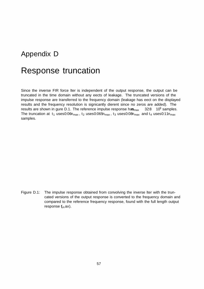
Appendix D
Response truncation
Since the inverse FIR force filter is independent of the output response, the output can betruncated in the time domain without any effects of leakage. The truncated versions of theimpulse response are transferred to the frequency domain (leakage has effect on the displayedresults and the frequency resolution is significantly different since no zeros are added). Theresults are shown in figure D.1. The reference impulse response has nmax “ 32.8ˆ 103 samples.The truncation at t1 uses 0.06nmax, t2 uses 0.065nmax, t3 uses 0.08nmax and t4 uses 0.11nmaxsamples.
t0t1t2
t3
t4
time rssÐÝfrequency rHzs
outp
utre
spon
se[m
/s2 ]
freq.
resp
onse
[m/(
s2N
)]Output responseTruncated FRReference FR
Figure D.1: The impulse response obtained from convolving the inverse filter with the trun-cated versions of the output response is converted to the frequency domain andcompared to the reference frequency response, found with the full length outputresponse (tmax).
57