NASA TECHNICAL NOTE

ti z c 4 w 4 z

DYNAMIC PERFORMANCE ANALYSIS OF A FUEL-CONTROL VALVE FOR USE I N AIRBREATHING ENGINE RESEARCH

by Peter G. Butterton und John R. Zeller

Lewis Research Center C Zeve land, Ohio

5331

N A T I O N A L A E R O N A U T I C S A N D SPACE A D M I N I S T R A T I O N W A S H I N G T O N , D . C. J U L Y 1 9 6 9

https://ntrs.nasa.gov/search.jsp?R=19690020599 2018-03-24T17:23:02+00:00Z

TECH LIBRARY KAFB, NM

DYNAMIC PERFORMANCE ANALYSIS OF A FUEL-CONTROL VALVE FOR

USE IN AIRBREATHING ENGINE RESEARCH

By Peter G. Batterton and John R. Zel le r

Lewis Resea rch Center Cleveland, Ohio

NATIONAL AERONAUTICS AND SPACE ADMINISTRATION ~~

For sal. by the CIoaringhouro for Federal Scientific and Technical lnformotion Springfiold, Virginia 22151 - CFSTI price $3.00

ABSTRACT

The analysis of a fast-response fuel-control valve for use in turbojet engine re- search is presented. This analysis includes cases where the valve is (1) closely coupled to the engine spray nozzles and (2) located some distance from the engine, thus require- ing connection by a hydraulic transmission line. The analysis results in a complete non- linear model and an equivalent linearized model for both cases. The dynamic perfor- mance of the analytical models is presented and compared against corresponding experi- mental fuel-flow response data. A discussion is included which demonstrates how oper- ating conditions affect fuel-flow frequency response.

ii

DYNAMIC PERFORMANCE ANALYSIS OF A FUELCONTROL VALVE

FOR USE IN AIRBREATHING ENGINE RESEARCH

by Peter G. Batterton and J o h n R. Ze l le r

Lewis Research Center

SUMMARY

An analysis of a fast-response fuel-control valve with a reducing pressure regulator is presented. This type of fuel-control valve is often used for dynamic and steady-state engine studies. A nonlinear analytical model for this valve is developed, which accur- ately predicts the dynamic performance of fuel flow from the valve in response to an in- put command. servo, this servo is not considered in this report. require that the fuel control be located some distance from the engine, thus requiring an interconnecting transmission line. line between the valve and the load.

A simplified linearized equivalent of the nonlinear analytical model is also derived and found to be an adequate representation for the valve. This linearized equivalent is particularly useful for the prediction of fuel-flow dynamic performance, both bandwidth and damping, for any load configuration. Also, the resulting transfer functions a r e use- ful in system performance evaluations. Results a r e included to demonstrate how this linear analytical model can be used to show some of the effects on the dynamic perform- ance due to various changes in operating parameters.

In addition, the t ime delay introduces an undesirable phase shift. tolerated for dynamic studies, but they seriously handicap the use of the valve in ad- vanced engine control systems. ever possible.

Since the fuel-flow response can be uncoupled from the valve actuating Many experimental configurations

The analysis is extended to include a transmission

The transmission line degrades the amplitude frequency response of the fuel system. Both effects can be

The use of a transmission line should be avoided when-

INTRODUCTION

Renewed interest in turbine engine research studies, both steady-state and dynamic,

has created a need for a fast-response, high-performance fuel-control valve. Such a de- vice should be able to (1) accurately control steady-state engine fuel flow and (2) provide controlled dynamic fuel-flow disturbances for the determination of the dynamic character- is t ics of various engine components. With these capabilities, the fuel-control valve can be employed within a control loop t o facilitate the evaluation of new and more sophisti- cated engine control concepts.

reducing fuel supply pressure to maintain a constant regulated pressure drop across a variable a r e a orifice best satisfies these requirements. The hydromechanical portion of this device controls output fuel flow in proportion to the a r e a of a fuel metering orifice and independent of output pressure. Metering orifice area is controlled by an electro- hydraulic servo actuation system. Fuel-control valve performance can be considered independently of the performance of the fuel valve servo. Thus, this report is re- stricted to fuel-flow performance with respect to a metering orifice a rea input.

In order to efficiently use this fuel-control valve fo r a specific application, it is necessary to understand and predict its dynamic performance for each set of operating conditions. To facilitate this understanding, we wil l present a detailed analysis of this hydromechanical control device operating directly into an orifice output termination (en- gine spray nozzles). Actual experimental installations often require the fuel-control de- vice to be located some distance from the spray nozzle load. Therefore, a long line is required to connect the two elements, and the dynamics of this transmission line wi l l be included in the analysis of the fuel-flow high-frequency dynamic performance. This in- clusion wi l l supplement the analysis presented in reference 1. To assist in predictions of dynamic performance, we wil l a lso derive a simplified linearized analytical model of this fuel-control valve and its connected load.

I

In reference 1, it w a s concluded that a fuel-control device based on the principle of I

PHYSICAL DESCRIPTION

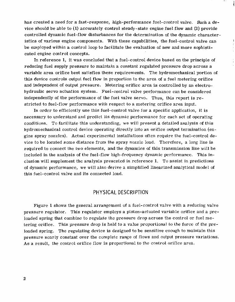
Figure 1 shows the general arrangement of a fuel-control valve with a reducing valve pressure regulator. This regulator employs a piston-actuated variable orifice and a pre- loaded spring that combine to regulate the pressure drop ac ross the control or fuel me- tering orifice. This pressure drop is held to a value proportional to the force of the pre- loaded spring. The regulating device is designed to be sensitive enough to maintain this pressure nearly constant over the complete range of flows and output pressure variations. As a result, the control orifice flow is proportional to the control orifice area.

2

High-pressure fue l supply i n p u t - actuator

Reducing valve or i f ice- c-c t T 7 1 Reducing valve piston- I-! A T o n t r o I or i f ice

Reducing valve spr ing- l--E $ C G o l l e d ou tpu t fuel flow

Figure 1. - Fuel-control valve wi th reducing valve pressure regulator.

ANALYTICAL DESCRl PTI ON

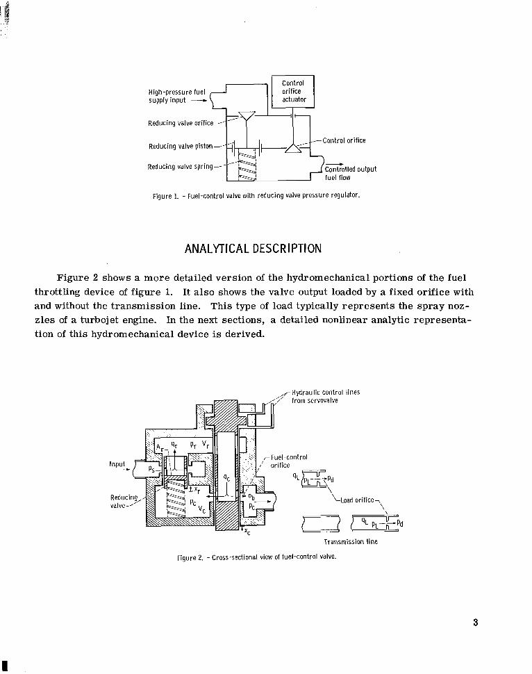
Figure 2 shows a more detailed version of the hydromechanical portions of the fuel throttling device of figure 1. It a lso shows the valve output loaded by a fixed orifice with and without the transmission line. This type of load typically represents the spray noz- z les of a turbojet engine. In the next sections, a detailed nonlinear analytic representa- tion of this hydromechanical device is derived.

,<Hydraulic control l ines / / / from servovalve

L L o a d orifice-,, \

Transmission l i n e

Figure 2. - Cross-sectional view of fuel-control Valve.

3

I

0 r i f ice Equations

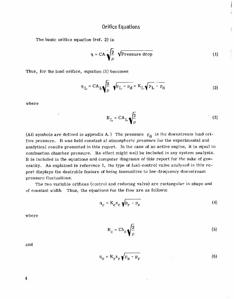
The basic orifice equation (ref. 2) is

q = CA$ 4Pressure drop

Thus, for the load orifice, equation (1) becomes

where

KL = C A L G (3)

(All symbols are defined in appendix A. ) The pressure pd is the downstream load ori- fice pressure. It was held constant a t atmospheric pressure for the experimental and analytical resul ts presented in this report. In the case of an active engine, it is equal to combustion chamber pressure. I ts effect might w e l l be included in any system analysis. It is included in the equations and computer diagrams of this report for the sake of gen- erality. A s explained in reference 1, the type of fuel-control valve analyzed in this re- port displays the desirable feature of being insensitive to low -frequency downstream p res sur e fluctuations.

of constant width. The two variable orifices (control and reducing valve) are rectangular in shape and

Thus, the equations for the flow are as follows:

where

K c = C h 8 C (5)

and

4

where

Kr = C h r e

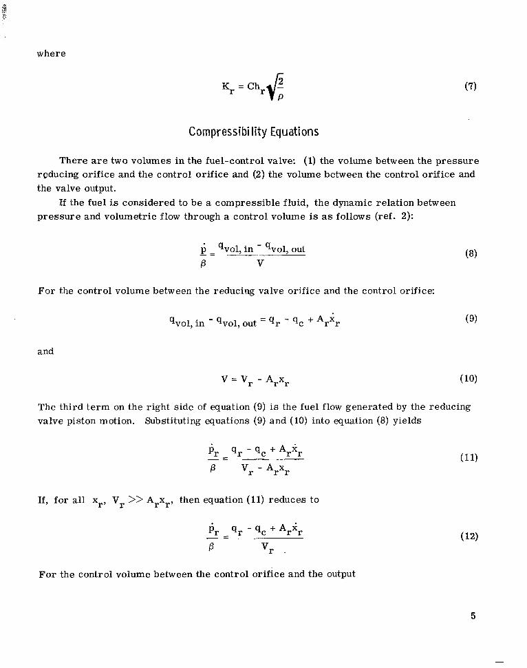
Compressibility Equations

There are two volumes in the fuel-control valve: (1) the volume between the pressure reducing orifice and the control orifice and (2) the volume between the control orifice and the valve output.

If the fuel is considered to be a compressible fluid, the dynamic relation between pressure and volumetric flow through a control volume is as follows (ref. 2):

For the control volume between the reducing valve orifice and the control orifice:

and

The third term on the right side of equation (9) is the fuel flow generated by the reducing valve piston motion. Substituting equations (9) and (10) into equation (8) yields

If, fo r all xr, V, >> Arxr, then equation (11) reduces to

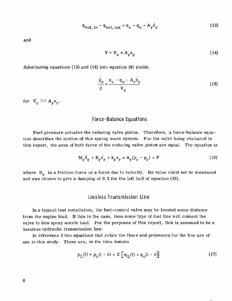
For the control volume between the control orifice and the output

5

and

V = V, i- Arxr

Substituting equations (13) and (14) into equation (8) yields

for V, >> Arxr.

Force-Balance Equations

Fuel pressure actuates the reducing valve piston. Therefore, a force-balance equa- tion describes the motion of this spring mass system. For the valve being evaluated in this report, the a r e a of both faces of the reducing valve piston a r e equal. The equation is

M 2 + Brgr + krxr = Ar(pC - p,) + F r r

where Br is a friction force o r a force due to velocity. Its value could not be measured and w a s chosen to give a damping of 0 .2 for the left half of equation (16).

Lossless Transmission Line

In a typical tes t installation, the fuel-control valve may be located some distance from the engine load. If this is the case, then some type of fuel line wi l l connect the valve to this spray nozzle load. 10s sle ss hydraulic transmission line.

use in this study.

For the purposes of this report, this is assumed to be a

In reference 3 two equations that relate the flows and pressures for the line a r e of These are , in the time domain

6

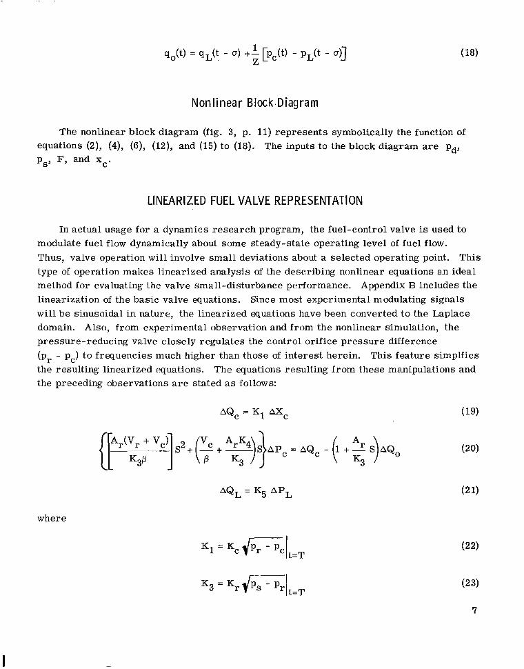
Nonl inear BIock.Diagram

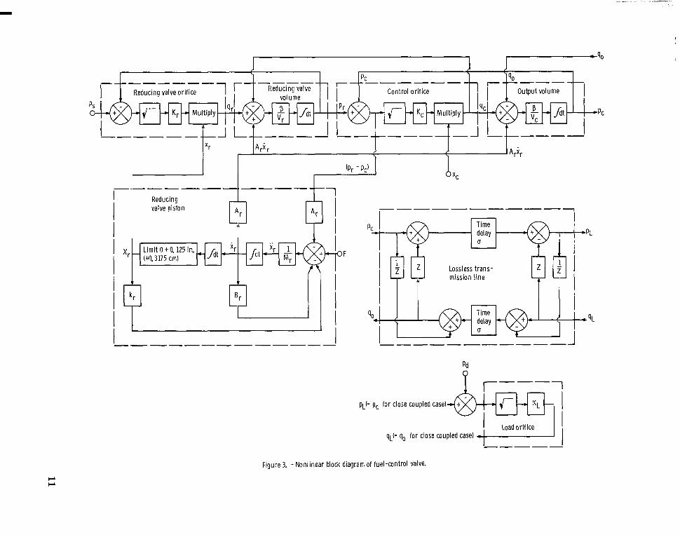
The nonlinear block diagram (fig. 3, p. 11) represents symbolically the function of equations (2), (4), (6), (12), and (15) to (18). The inputs to the block diagram are pd, Ps, F, and xc.

LINEARIZED FUEL VALVE REPRESENTATION

In actual usage for a dynamics research program, the fuel-control valve is used to modulate fuel flow dynamically about some steady-state operating level of fuel flow. Thus, valve operation w i l l involve small deviations about a selected operating point. type of operation makes linearized analysis of the describing nonlinear equations an ideal method for evaluating the valve small-disturbance performance. Appendix B includes the linearization of the basic valve equations. w i l l be sinusoidal in nature, the linearized equations have been converted to the Laplace domain. Also, from experimental observation and from the nonlinear simulation, the pressure- r educing valve closely regulates the contr ol orif ice pressure difference (p, - pc) to frequencies much higher than those of interest herein. the resulting linearized equations. the preceding observations a r e stated as follows:

This

Since most experimental modulating signals

This feature simplfies The equations resulting from these manipulations and

{ p ( y c j S + (; - + - S A P A;;)} c = A Q c - ( l + - - S A Q o :; )

where

I

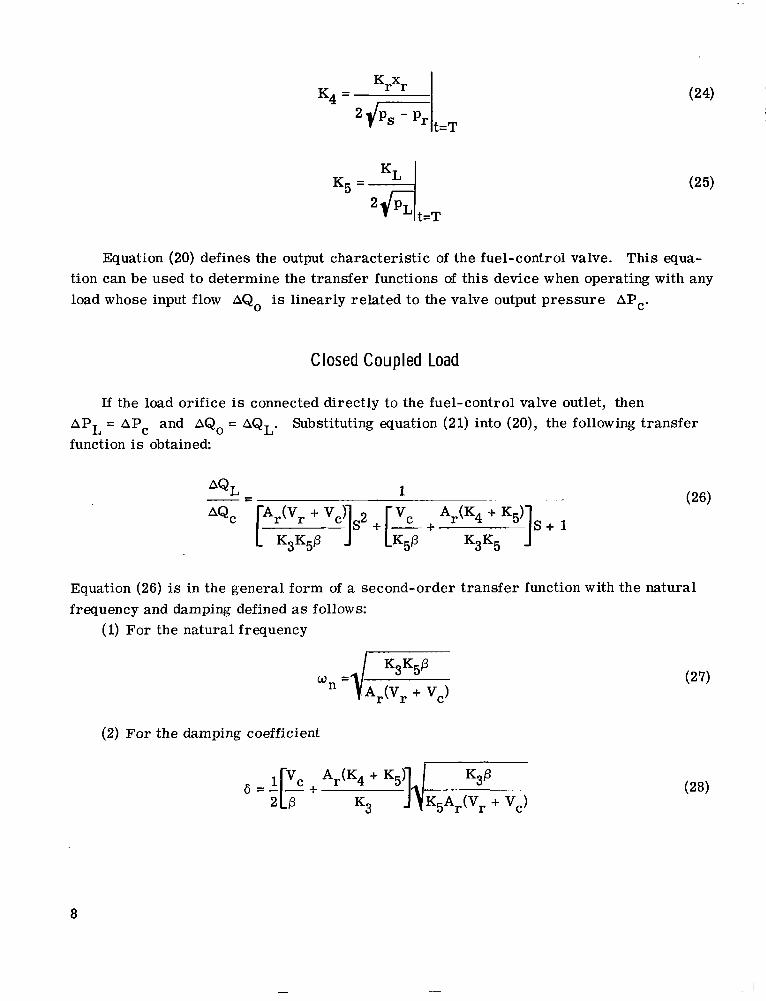
Equation (20) defines the output characterist ic of L e &;lel-control valve. This equa- tion can be used to determine the transfer functions of this device when operating with any load whose input flow AQo is linearly related to the valve output pressure APc .

Closed Coupled Load

If the load orifice is connected directly to the fuel-control valve outlet, then A P L = A P c and AQo = AQL. function is obtained

Substituting equation (21) into (20), the following transfer

AQL - 1 --

Equation (26) is in the general form of a second-order t ransfer function with the natural frequency and damping defined as follows:

(1) For the natural frequency

(2) For the damping coefficient

8

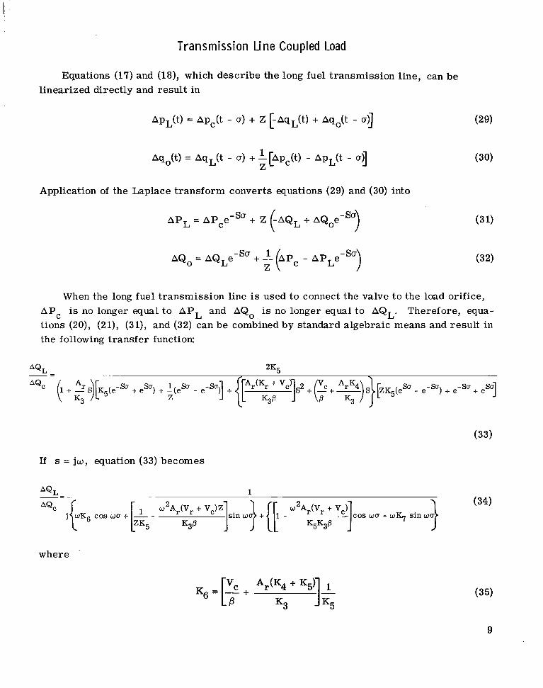
Transmission Line Coupled Load

Z

Equations (17) and (18), which describe the long fuel transmission line, can be linearized directly and result in

Application of the Laplace transform converts equations (29) and (30) into

A P L = APce-Sa + Z (3 1)

AQo = AQLe -Sa + - 1 (4Pc - APLe-'O) Z

When the long fuel transmission line is used to connect the valve to the load orifice, A P c is no longer equal to A P L and AQo is no longer equal to AQL. Therefore, equa- tions (20), (21), (31), and (32) can be combined by standard algebraic means and result in the following transfer function:

If s = ju, equation (33) becomes

where

(35)

9

and

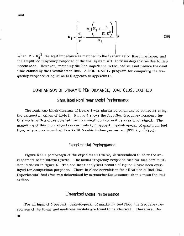
K7=

-

-+ vC P Ark4+*)] K3 Z

COMPARISON OF DYNAMIC PERFORMANCE, LOAD CLOSE COUPLED

Simulated Nonlinear Model Performance

The nonlinear block diagram of figure 3 w a s simulated on an analog computer using the parameter values of table I. Figure 4 shows the fuel-flow frequency response for this model with a close coupled load to a small control orifice area input signal. The magnitude of this input signal corresponds to 5 percent, peak-to-peak, of maximum fuel flow, where maximum fuel flow is 38. 5 cubic inches per second (630. 9 cm /sec). 3

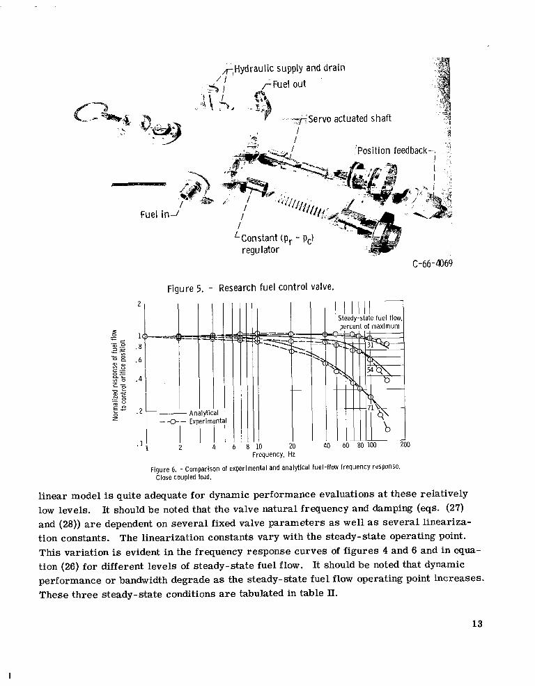
Experimental Performance

Figure 5 is a photograph of the experimental valve, disassembled to show the ar- rangement of its internal parts. The actual frequency response data for this configura- tion is shown in figure 6. The nonlinear analytical resul ts of figure 4 have been over- layed for comparison purposes. There is close correlation for all values of fuel flow. Experimental fuel flow w a s determined by measuring the pressure drop across the load or if ic e.

Linearized Model Performance

For an input of 5 percent, peak-to-peak, of maximum fuel flow, the frequency r e - sponses of the linear and nonlinear models a r e found to be identical.

10

Therefore, the

- 1 Reducing valve piston

- .

-At - Limit 0 t 9. 125 in. (+I 3175 cm) -

1

I F

Time delay

PC

U

Loss1 ess trans- mission l i n e

T r--- 1 p ~ ( = pc for close coupled case)

Load ori f ice qL(= qo for close coupled case)

Figure 3. - Nonlinear block diagram of fuel-control valve.

Frequency, Hz

Figure 4. - Fuel-flow frequency response from simulated nonl inear model. Close coupled load.

TABLE I. - FUEL CONTROL VALVE MECHANICAL CONSTANTS ~~ _ _ ~

2 Reducing valve piston area, in. ’; cm

Reducing valve friction, B, (lbf)(sec)/in, ; (N)(sec)/cm

Reducing valve spring bias, F, Ibf; N

Control orifice constant, Kc, in. 3/(sec)(lbf1/2); cm3/(sec)(N1/’) Load orifice constant, KL, in. 4/’(sec)(lbf1/2); em 4 /(sec)(N1/’)

Reducing valve orifice constant, Kr’ in. 3/(sec)(lbf1/2); em 3 /(sec)(N1l2)

Reducing valve spring constant, k r , lbf/in. ; N/cm

Reducing valve piston mass , Mr, (lbf)(sec )/in. ; (N)(sec )/cm 2 Fuel supply pressure , p,, psi; N/cm 3 Control orifice volume, vC, in. 3; cm

Reducing valve volume, Vr, in. 3; cm3

Hydraulic l ine su rge impedance, 2 , (lbf)(sec)/in. 5; (N)(sec)/cm

Fuel bulk modulus, p, psi; N/cm

Fuel mass density, p , (lbf)(sec )/in. , (N)(sec )/cm

Hydraulic t ime delay, u, s ec

Hydraulic line area, a, in. ’; cm

Zydraulic line length, I , in. ; cm

2 . 2

5

2

2 . 4. 2 4

2

- _. - .-

1.0; 6.45

0.0633; 0.1109

140; 623

16.25; 126.26

1.397; 27. 57

70.4; 547.0

100; 175

2 . 5 1 ~ 1 0 - ~ ; 4 .40

650; 448

7.5; 122.9

5.55; 90.95

9.235; 16. 18

1 . 5 ~ 1 0 ~ ; 1 . 0 4 ~ 1 0 ~

7 . 5 ~ 1 0 ~ ~ ; 8. 0 2 ~ 1 0 - ~

2. 6X10-3

0.36317; 2. 343

120; 305

12

- T,Hydraulic supply and drain fi

/ I 5/ r-Fuel out

-TrServo actuated shaft I

C-66-4069

Figure 5. - Research fuel control valve.

2 4 6

I I I I I 1 1 1 1 I 1 Steady-state fuel flow,

a Frequency, Hz

Figure 6. - Comparison of experimental and analyt ical fuel-flow frequency response. Close coupled load.

linear model is quite adequate for dynamic performance evaluations at these relatively low levels. It should be noted that the valve natural frequency and damping (eqs. (27) and (28)) a r e dependent on several fixed valve parameters as well as several lineariza- tion constants. The linearization constants vary with the steady-state operating point. This variation is evident in the frequency response curves of figures 4 and 6 and in equa- tion (26) for different levels of steady-state fuel flow. It should be noted that dynamic performance or bandwidth degrade as the steady-state fuel flow operating point increases. These three steady-state conditions are tabulated in table II.

13

I

TABLE I[. - FUEL CONTROL VALVE OPERATING CONDITIONS

[Maximum fuel flow, 38.5 in. 3 / sec (10.0 gal/min o r 630.9 cm 3 /sec); fuel supply pressure , 650 psi (448 N/cm 2 ). 3

Pe rcen t Reducing Control Control orifice Reducing valve

F - F e ; ? , p re s su re , p re s su re , orifice I length,

31 213 147 73 50 6 3 ~ 1 0 - ~

54 362 250 222 153 109

7 1 523 361 383 264 144

DYNAMIC PERFORMANCE WITH

X I

1.57 8 . 1 3 ~ 1 0 - ~ 0.206

2.77 17.38 .441

3.66 34.15 .867

A LONG LINE

Performance of S i m u lated Model

The nonlinear block diagram of figure 3 w a s simulated on an analog computer using the parametric values of table I. The 2.6-millisecond time delay w a s simulated with a fourth-order Pade approximation (ref. 4). Dynamic performance w a s evaluated for the case of a 10-foot (3.048-m) long, 0.75-inch (1.905-cm) outside diameter, stainless-steel fuel transmission line at 54-percent maximum steady-state fuel flow using the same load orifice as the close coupled case. The performance of the close coupled nonlinear model a t 54-percent maximum fuel flow is overlayed for demonstration purposes. The effect of the transmission line is consid- erable, degrading the system bandwidth by nearly a 4 to 1 margin.

The performance f o r this condition is given in figure 7.

Transmission lin Close coupled load

4 2 4 6 8 1 0 20 40 60 80 I-; I I I I

Frequency, Hz

Figure 7. - Comparison of non l inear model fuel-flow frequency responses for close coupled and transmission l i n e coupled load. Steady-state fuel flow, 54 percent maximum.

14

Experimental Performance

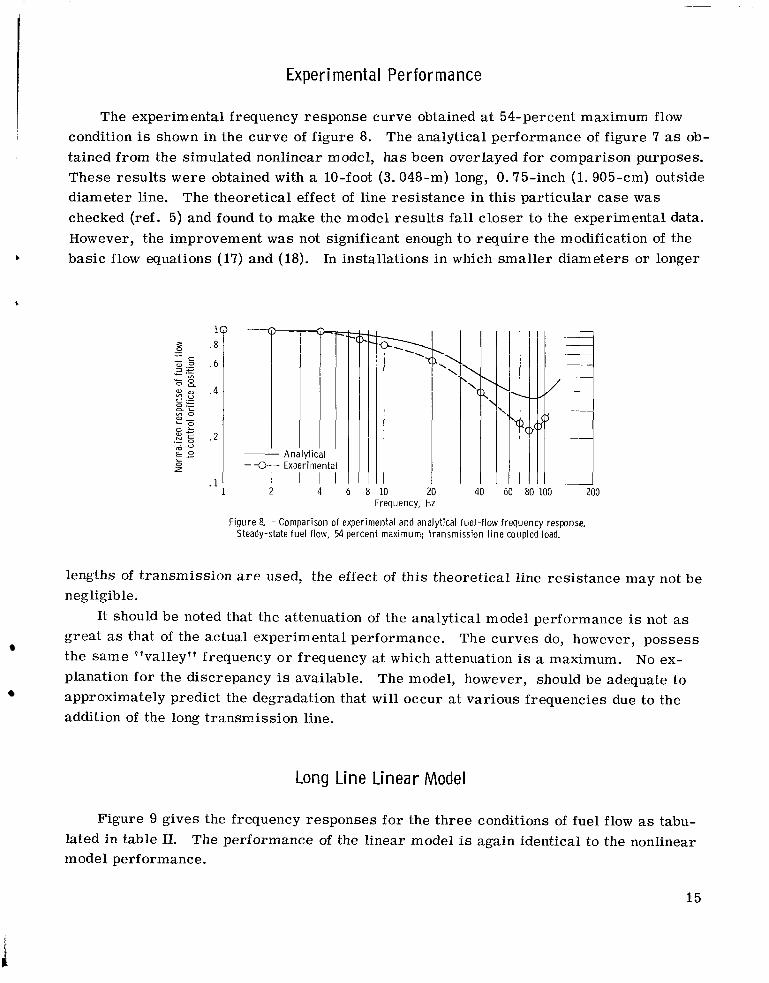
The experimental frequency response curve obtained at 54-percent maximum flow condition is shown in the curve of figure 8. The analytical performance of figure 7 as ob- tained from the simulated nonlinear model, has been overlayed for comparison purposes. These resul ts w e r e obtained with a 10-foot (3.048-m) long, 0.75-inch (1.905-cm) outside diameter line. The theoretical effect of line resistance in this particular case w a s checked (ref. 5) and found to make the model resul ts fall closer to the experimental data. However, the improvement was not significant enough to require the modification of the

I

b basic flow equations (17) and (18). In installations in which smaller diameters or longer

1 A n

-Q- Experimental I I l l I:: 1

1 2 4 6 8 1 0 20 40 60 80 100 200 Frequency, Hz

Figure 8. - Comparison of experimental and analytical fuel-f low frequency response. Steady-state fuel flow, 54 percent maximum; transmission l i n e coupled load.

lengths of transmission are used, the effect of this theoretical line resistance may not be negligible.

great as that of the actual experimental performance. the same vevalley" frequency o r frequency at which attenuation is a maximum. planation for the discrepancy is available.

addition of the long transmission line.

It should be noted that the attenuation of the analytical model performance is not as The curves do, however, possess

No ex- The model, however, should be adequate to

approximately predict the degradation that wi l l occur a t various frequencies due to the

Long Line Linear Model

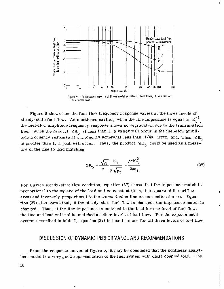
Figure 9 gives the frequency responses for the three conditions of fuel flow as tabu- The performance of the linear model is again identical to the nonlinear lated in table 11.

model performance.

15

P ! D

T

6 8 10' 20 40 60 80 100 200 Frequency, Hz

Figure 9. - Frequency response of l inear model at dif ferent fue l flows. Transmission l i n e coupled load.

Figure 9 shows how the fuel-flow frequency response varies at the three levels of steady-state fuel flow. As mentioned earlier, when the line impedance is equal to K i l the fuel-flow amplitude frequency response shows no degradation due to the transmission line. When the product ZK5 is less than 1, a valley wi l l occur in the fuel-flow ampli- tude frequency response at a frequency somewhat less than 1/40. hertz, and, when ZK is greater than 1, a peak wil l occur. Thus, the product ZK5 could be used as a meas- u re of the line to load matching

?

5

2 fi KL -PCKL ZK5=-- -~

a 2 6 L 2aqL (37)

For a given steady-state flow condition, equation (37) shows that the impedance match is proportional to the square of the load orifice constant (thus, the square of the orifice area) and inversely proportional to the transmission line cross-sectional area. Equa- tion (37) also shows that, i f the steady-state fuel flow is changed, the impedance match is changed. the line and load wi l l not be matched a t other levels of fuel flow. system described in table I, equation (37) is less than one for all three levels of fuel flow.

b

b

Thus, if the line impedance is matched to the load for one level of fuel flow, For the experimental

DISCUSSION OF DYNAMIC PERFORMANCE AND RECOMMENDATIONS

From the response curves of figure 5, it may be concluded that the nonlinear analyt- ical model is a very good representation of the fuel system with close coupled load. The

16

j I '

20x102

500 600 700 800 Supply pressure, ps, psi

I 400 500

I 300

Supply pressure, ps, Nlcm2

constant at 1.397 inch4 per second per pound1/2 (27.54 cm4/(sec)(NU2)).

I I 100 200

Figure 10. - Effect of supply pressure on valve natura l frequency. Load or i f ice

100 80

60

40

20

to

c a c

'U ._ 10 8 8 I - " m

a

m

._ c 6

n 4 E

2

1 . 8

.6 100

\

200 300 400

\.

-_ 1

800 Supply pressure, ps, psi

J 100 200 300 400 500

Supply pressure, ps, N/cm*

I

Figure 11. - Eff c t of supply pressure o valve damping. Load or i f ice constant at 1.397 i n c h t per second per pound j2 (27.57 cm4/(sec)(NU2)).

17

second-order linear t ransfer function describing this configuration also accurately repre- sents the dynamic system. The main advantage of the t ransfer function linearization is that the fuel system flow response for various conditions can be predicted almost by in- spection.

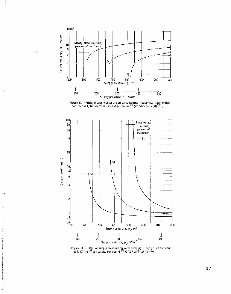
Both parameters affect the values of w n and 6, the natural frequency and damping of the valve. Figures 10 and 11 show how wn and 6 vary, respectively, as functions of the supply pressure with a specific load orifice constant. The value of KL is 1.397 inch per second per pound1l2 (27.5 cm /(sec)(N1/2)). W e can see that, as the supply pressure is decreased, w n decreases and damping increases. the dynamic performance capabilities of the fuel valve. Thus, to operate unattenuated to the highest frequencies, supply pressure should be maintained at the higher level (650 to 800 psi (450 to 550 N/cm2)).

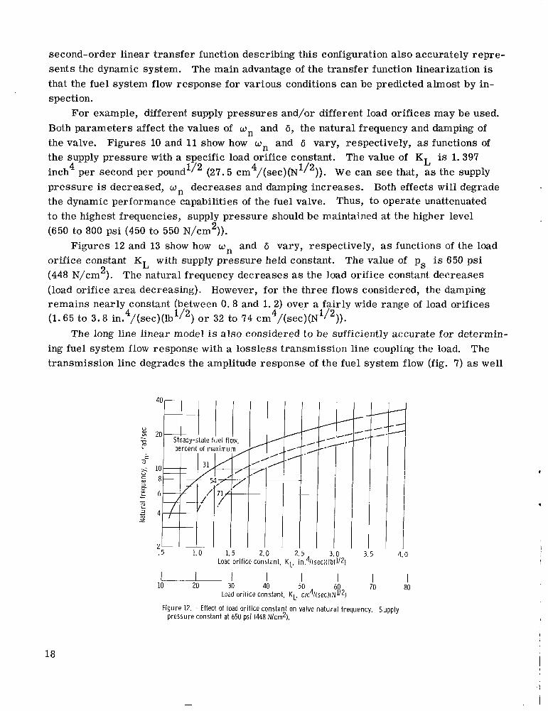
orifice constant KL with supply pressure held constant. The value of ps is 650 psi (448 N/cm2). The natural frequency decreases as the load orifice constant decreases (load orifice a rea decreasing). However, for the three flows considered, the damping remains nearly constant (between 0.8 and 1.2) ove,r a fairly wide range of load orifices

For example, different supply pressures and/or different load orifices may be used.

4 4

Both effects wil l degrade

Figures 12 and 13 show how w n and 6 vary, respectively, as functions of the load

(1.65 to 3.8 in. 4 /(sec)(lb1/2) o r 32 to 74 cm 4 /(sec)(N1/2)).

The long line linear model is also considered t o be sufficiently accurate for determin- ing fuel system flow response with a lossless transmission line coupling the load. The transmission line degrades the amplitude response of the fuel system flow (fig. 7) as well

3.0 3.5 Load ori f ice constant, KL, in.4/(sec)(lbfU2)

I 70

I 60

I 50

I 40

-1- 10 20 30

Load orif ice constant, Kb c ~ n ~ / l s e c ) ( N ~ / ~ )

4.0

I 80

Figure 12. - Effect of load ori f ice constant on valve na tu ra l frequency. Supply pressure constant at 650 psi (448 N/cmZ).

18

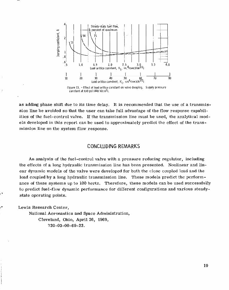
. 6 l .5

-

, 54 \

'\

I 10

Steady-state fuk l flow, percent of maximum

- - '2

1.5 2.0 2.5 3.0 Load or i f ice constant, KL, in4/(sec)( lbf1/2)

1-

3.5 0

I 6 70 80 1% Load or i f ice constant, KL, cm4/(sec)(N 1

I 50

I 40

1 30

Figure 13. - Effect of load or i f ice constant on valve damping. Supply pressure constant at 650 psi 1448 N/cmZ).

as adding phase shift due to its time delay. sion line be avoided so that the user can take full advantage of the flow response capabil- i t ies of the fuel-control valve. els developed in this report can be used to approximately predict the effect of the t rans- mission line on the system flow response.

It is recommended that the use of a transmis-

If the transmission line must be used, the analytical mod-

C ONC LU D IN G REMARKS

An analysis of the fuel-control valve with a pressure reducing regulator, including the effects of a long hydraulic transmission line has been presented. e a r dynamic models of the valve were developed for both the close coupled load and the load coupled by a long hydraulic transmission line. These models predict the perform- ance of these systems up t o 100 hertz. Therefore, these models can be used successfully t o predict fuel-f low dynamic performance for different configurations and various steady-

Nonlinear and lin-

I state operating points. 17

I * Lewis Research Center, I

I National Aeronautics and Space Administration, Cleveland, Ohio, April 26, 1969,

720-03-00-69-22.

19

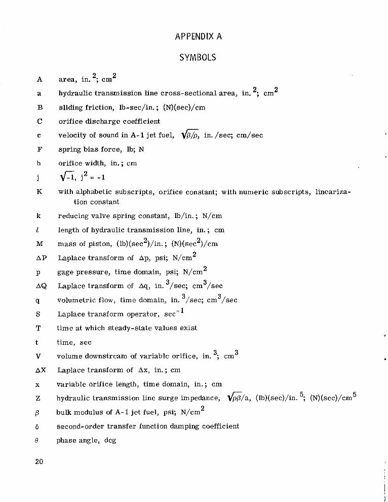
APPENDIX A

SYMBOLS

A

a

B

C

C

F

h

j

K

k

1

M

A P

P

AQ

q

S

T

t

V

AX

X

Z

P 6

e

2 area, in. 2; cm 2 hydraulic transmission line cross-sectional area, in. 2; cm

sliding friction, lb-sec/in. ; (N)(sec)/cm

orifice discharge coefficient

velocity of sound in A-1 jet fuel, 6, in. /sec; cm/sec

spring bias force, lb; N

orifice width, in.; cm

fi, j2 = -1

with alphabetic subscripts, orifice constant; with numeric subscripts, lineariza- tion constant

reducing valve spring constant, lb/in. ; N/cm

length of hydraulic transmission line, in. ; cm mass of piston, (lb)(sec 2 )/in. ; (N)(sec2)/cm

2 Laplace transform of Ap, psi; N/cm

gage pressure, t ime domain, psi; N/cm

Laplace transform of Aq, in. /sec; cm /sec 3 3 volumetric flow, time domain, in. /sec; cm /see

Laplace transform operator, see-'

time at which steady-state values exist

2

3 3

time, sec

volume downstream of variable orifice, in. 3; cm

Laplace transform of Ax, in.; cm

variable orifice length, time domain, in. ; cm

3

5 hydraulic transmission line surge impedance, G / a , (lb)(sec)/in. 5; (N)(sec)/cm 2 bulk modulus of A-1 jet fuel, psi; N/cm

second-order transfer function damping coefficient

phase angle, deg

20

2 2 4 P

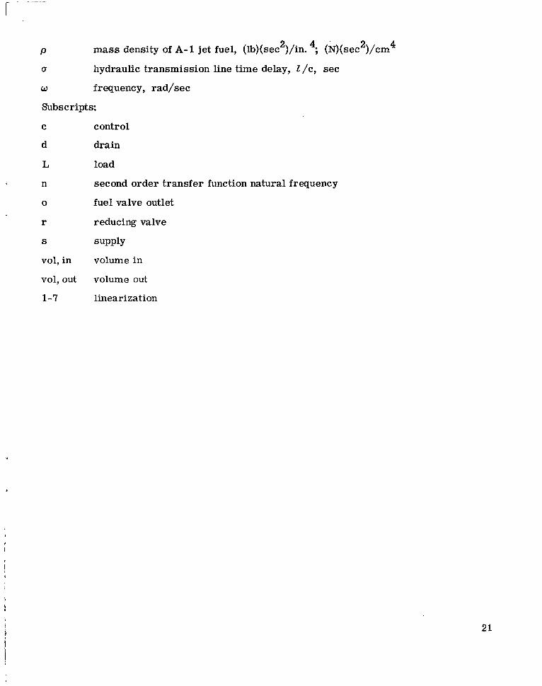
5 hydraulic transmission line time delay, Z/c, sec

0 frequency, rad/sec

Subscripts:

mass density of A-1 jet fuel, (lb)(sec )/in. 4; (N)(sec )/cm

C

d

L

n

0

r

S

v01, in

v01, out

1-7

c ont r ol

drain

load

second o r L x transfer ,mction natural frequency

fuel valve outlet

reducing valve

supply

volume in

volume out

linearization

Y

21

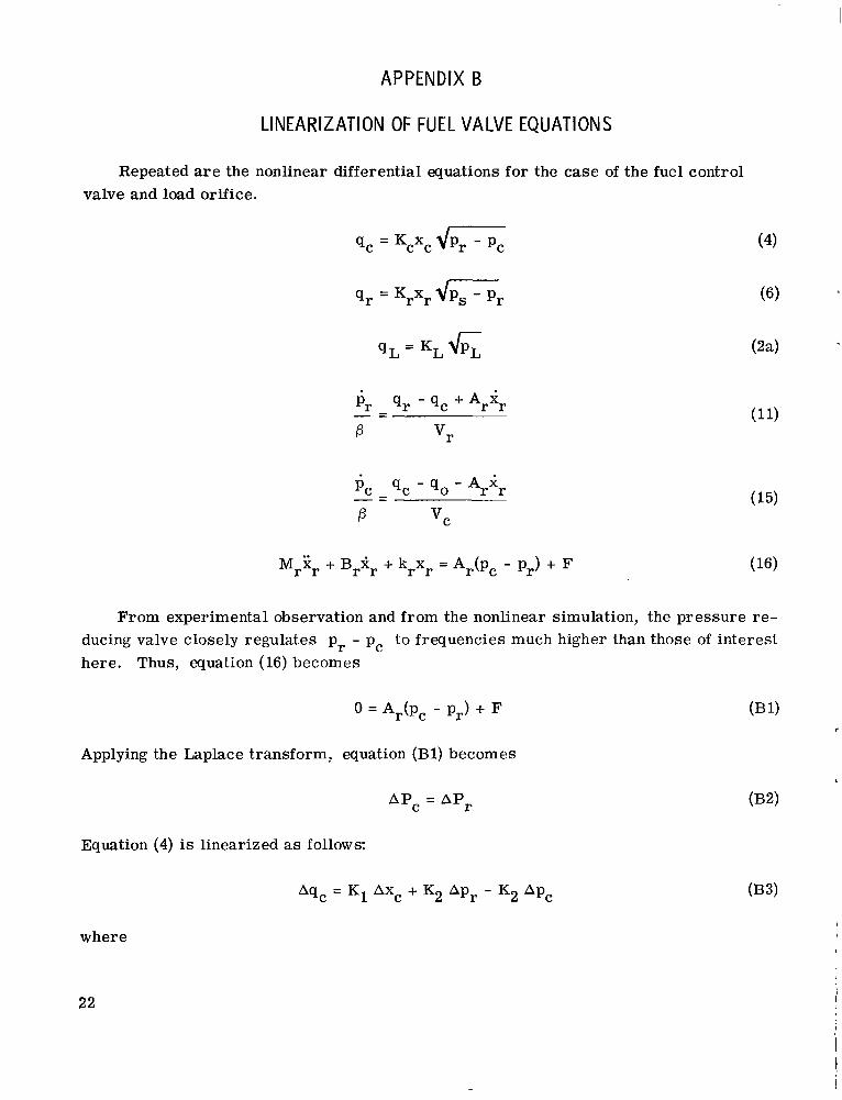
APPENDIX B

LINEARIZATION OF FUEL VALVE EQUATIONS

Repeated a r e the nonlinear differential equations for the case of the fuel control valve and load orifice.

qC = K c X c d - P ,

qr = KrXrJPs - P,

(4)

MrZr + Br i r + krXr = Ar(pc - pr) + F (16)

From experimental observation and from the nonlinear simulation, the pressure re- ducing valve closely regulates p, - p, to frequencies much higher than those of interest here. Thus, equation (16) becomes

0 = Ar(Pc - P,) + F

Applying the Laplace transform, equation (Bl) becomes

AP, = A P r

Equation (4) is linearized as follows:

where

22

K1 = Kc

1 1 K2 = z KcXc fi

and

t=T

Applying the Laplace transform and substituting equation (B2) yields for equation (B3)

AQc = K1 AX, (19)

In the same manner, equations (6) and (2a) are linearized as follows:

where

and

. where

1

t=T

1

I

Applying the Laplace transform yields for equations (B5) and (B6)

I j AQr = K3 AX, - Kq AP,

where

23

and

where

A P r = A P c

AQL = K5 A P L

Similarly, equations (11) and (15) yield

APC&= AQr - AQc + SA, AXr P

A P r = A P c

APcS -- vc - AQc - AQo - SA, AX, P

By standard algebraic methods, equations (B7), (B9), and (B10) can be reduced to yield the following equation:

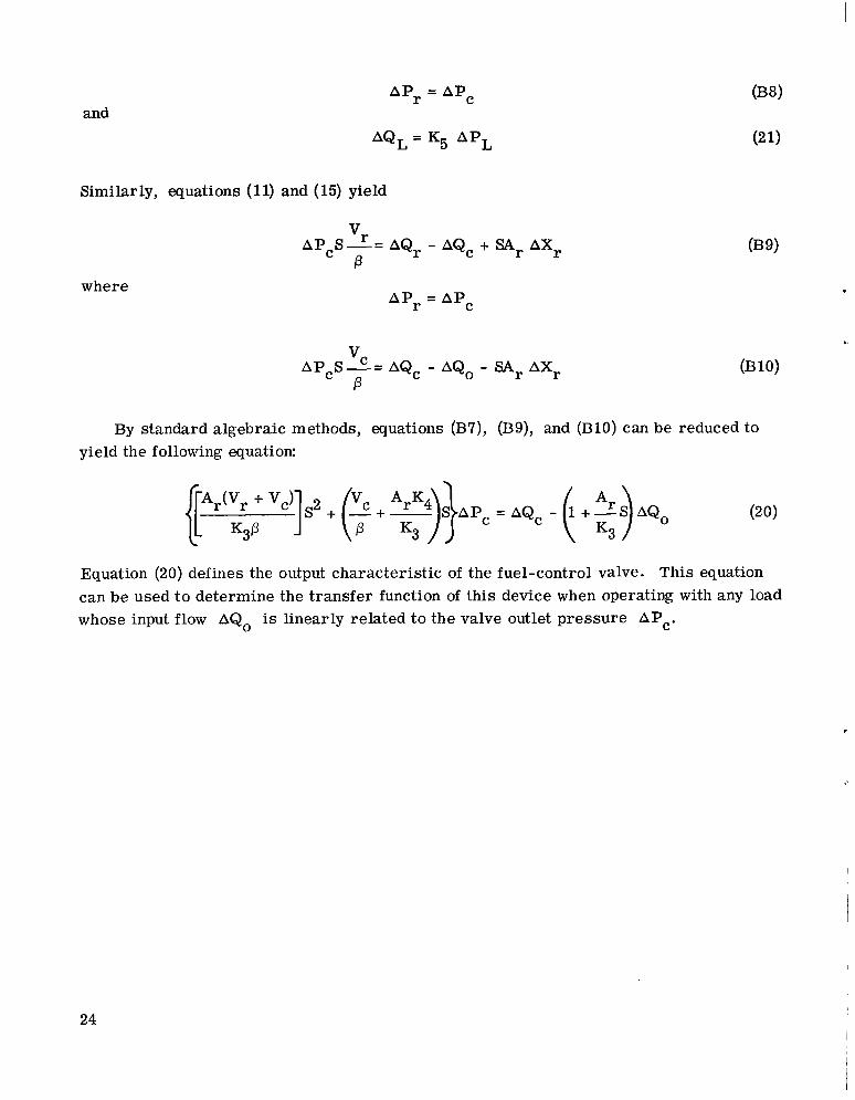
Equation (20) defines the output characteristic of the fuel-control valve. This equation can be used to determine the transfer function of this device when operating with any load whose input flow AQo is linearly related to the valve outlet pressure APc.

24

APPENDIX C

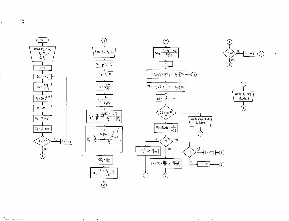
DIGITAL COMPUTER PROGRAM AND FLOW DIAGRAM

25

Read P,, Z, (I, KL, K,, v,. v,,

P, A,

b i = 1

I

c i = cos wi(I

S i = s i n wio

i = 25?

Read P,, P,, xr i SQ =m x K3 = K,SQ

/I K4 '2SQ

G S = TI^ t T R ~ I 4

Write magnitude to large

1 Magnitude = - m

p-t@ Yes

Wri te fi, mag-

REFERENCES

1. Otto, Edward W. ; Gold, Harold; and Hil ler , Kirby W. : Design and Performance of Throttle-Type Fuel Controls for Engine Dynamic Studies. NACA TN 3445, 1955.

2. Stenning, A. H. ; and Shearer, J. L. : Fundamentals of Fluid Flow. Fluid Power Control. John F. Blackburn, Gerhard Reethof, and J. Lowen Shearer, eds., Technology Press of M. I. T. and John Wiley & Sons, Inc., 1960, ch. 3, sec. 3.3.

3. Ezekiel, F. D. ; and Paynter, H. M. : Fluid-Power Transmission. Fluid Power Con- trol. John F. Blackburn, Gerhard Reethof, and J. Lowen Shearer, eds., Tech nology P r e s s of M.I.T. and John Wiley & Sons, Inc., 1960, ch. 5, sec. 5.3.

4. Carlson, Alan; Hannauer, George; Carey, Thomas; and Holsberg, Peter J., eds. : Handbook of Analog Computation. Second ed., Electronics Associates, Inc., 1965.

5. Karam, J. T. , Jr. : A New Model for Fluidics Transmission Lines. Control Eng., vol. 13, no. 12, Dec. 1966, pp. 59-63.

NASA-Langley, 1969 - 3 E-5019 27