AD-A012 581

VLF AIRBORNE NAVIGATION REQUIREMENTS

E. R. Swanson, et al

Naval Electronics Laboratory Center

Prepared for:

Federal Aviation Administration

15 January 1975

DISTRIBUTED BY:

National Technical Information Service U. S. DEPARTMENT OF COMMERCE

Report No. FA74WÄI 425-1

Naval Electronics Laboratory Center TR 1941

211147

VLF AIRBORNE NAVIGATION REQUIREMENTS

00 to

o <

E. R. SWANSON

M. J. DICK

15 JANUARY 1975

FINAL REPORT

Document is available to the public through the National Technical Information Service,

Springfield, Virginia 22151

Prepared for

U.S. DEPARTMENT OF TRANSPORTATION FEDERAL AVIATION ADMINISTRATION

Systems Research & Development Service Washington, D.C. 20590

NATIONAL TECHNICAL INFORMATION SERVICE

US Dttpartmonl °* Common:«« Sprmgfifcld, VA 22151

Ttehnicol tfcport Documentation Page

1. Report No.

FA74WAI425-1

2. Gov«frtmen» Accession No. 3. Recipient » Catalog No.

4. y tie ond Subtitle

VLF AIRBORNE NAVIGATION REQUIREMENTS

5. Report Dote

15 January 1975 6. Performing Organization Cod«

7. Author's)

E. R. Swanson and M. J. Dick

J 8. Performing Orgonizotion Report No.

NELC Technical Report 1941 (TRI94I)

9. Performing Orgonnotjon Nome ond Address

Naval Electronics Laboratory Center San Diego, California 92152

10. Work Unit No (TRAIS)

ii. Contract or Gron» No.PAA Inter. DOT-FA 74WAI425 (NELC A208)

12. Sponsoring Agency Nome and Address

Federal Aviation Administration

13. Type of Report ond Period Coverad

Final Report I December 1973 to December 1974

14. Sponsoring Agency Code

15. Suoplementory Notes

16. Abstroct

A mathematical analysis of safety within the airways is presented with special attention to the interrelationship be- tween pilotage errors and navigational errors characteristic of some vlf navigational methods. Error probability convolutions are performed. It is concluded that an error budget of 3.5 nmi fo, the vlf navigation system will provide adequate safety, but continued experimental work on error distribution and the performance of additional error convolutions and safety evaluations are recommended.

17. Key Words

Navigation Safety Air Navigation Navigation Vlf

Omega Very low frequencies

19. Security Clossif. (of this report)

Unclassified

18, Distribution Statement

Document is available to the public through the National Technical Information Service. Springfield, Virginia 22151

20. Security Clossif. (of this page)

Unclassified

21. No. of Pog*» .2. Pnci

^>-> 3f^T~ j Form DOT F 1700.7 (8-72) Reproduction of competed page author,zed ^ HiCES SUBJECT TO CHANGE

^■ar^s^s^^r^it'^ ^"^

I ■

OBJECTIVE

Determine accuracy requirements for a vlf navigation eystem providing capability for safe aircraft operation within existing airways.

RESULTS

1. Various scenarios for possible aircraft operation using vlf navigation were con- sidered. These included both "Omega type" fixing and initialization procedures.

2. Vlf error characteristics can be arranged so that they are bounded if signals are monitored for protection against sudden propagational anomalies.

3. Various error sources were convoluted to obtain expected aircraft error distri- bution functions.

4. An error budget of 3.5 nmi for the vlf navigation system will provide adequate safety.

RECOMMENDATIONS

1 Continue experimental work on error distribution. (The difficulty of ade- quately determining statistics on unusually large deviations is acknowledged.)

2. Perform many more error convolutions and safety evaluations a professional lifetime spent assessing these errors would be most useful.

ADMINISTRATIVE INFORMATION

Work was performed under the cognizance of G. Quinn under Federal Aviation Ad- ministration Interagency Agreement DOT-FA 74WA1-425 (NELC A208) from December 1973 to December 1974. This report was completed in December 1974 and approved for publication 31 December 1974.

REVERSE SIDE BLANK

CONTENTS

INTRODUCTION ... page 7

AIRWAY STRUCTURE... 8

VLF ERRORS ... 8

PILOTAGE ERRORS... 13

ACCURACY CRITERION ... 14

ERROR SYNTHESIS ... 17

CONCLUSIONS... 21

REFERENCES... 21

ILLUSTRATIONS

1. Idealized error distributions .. . page 10 2. Simplified sum of two modes... 11 3. Model for errors due to modal interference ... 12 4. Development of collision risk ... 14 5. Error convolutions ... 18 6. Safety associated with various error structures ... 20

TABLES

1. Relative collision probabilities ... page 16 2. Navigational error characteristics for safe operation with a =* 1 /2 nmi

Gaussian pilotage error... 21

REVERSE SIDE BLANK

M

i i

t I

V

INTRODUCTION

Safety and accuracy are sometimes erroneously equated by the layman. In practice, excessive navigational accuracy can foster unsafe conditions. As a trivial example» suppose two aircraft assigned the same flight level are over the same point at the same time. If both are carefully piloted and equipped with precision altimeters, a collision will have occurred. If, however, both have rather poor altimeters, there is a good chance one aircraft will be above the other and hence they may miss. Excessive navigational precision allows the coalescence of traffic to hazardous densities.

| Air traffic safety, especially across the North Atlantic, has received considerable at- | tention, particularly from Reich in the United Kingdom and Braverman in the United States. I A paper by Braverman' provides an especially good introduction to the relationship between

navigational safety and accuracy. Safety must be designed into air traffic systems. Follow- | ing the risk acceptance model of Starr, Braverman has shown that the maximum acceptable | interval between collisions across the North Atlantic is 1200 years! Quite apparently, ade- | quate collision statistics will not be available for an empirical assessment. ! Braverman draws an important distinction between "primitive" and "nonprimitive" | systems. In primitive systems, for which the separation standard may be less than about five

standard deviations of normal error, accidents may often be caused by lack of accuracy. In f these systems, protection is needed against the usual. In nonprimitive systems, for which | the separation standard is greater than five standard deviations of normal error, accidents

will be primarily caused by unexpected and undetected large errors or "blunders." * - For J such systems protection is needed only against the "unusual."

It must be understood that the effective criterion in separating primitive from non- primitive systems is fundamentally whether or not the system is usually safe. A hypothetic

1 cal system which insured that under no circumstances was an aircraft off track by more than one-half the airway spacing would likely be safe even if it uniformly distributed aircraft up to plus or minus half the separation distance. Indeed, uniformly distributing similarly directed traffic over a region is beneficial in that it reduces the probability of overtaking collisions. The separation criterion thus depends on the statistical nature of the errors as well as the accuracy as expressed by the standard deviation. For example, the bounded system with uniformly distributed error previously considered would exhibit an rms lateral fixing error of 0.29 of the traffic separation. The system would be safe even though the spacing was only about 3.4 standard deviations. The proper interpretation of the "5 sigma" criterion is that the actual collision probability is that associated with two normally dis- tributed error functions with standard deviations equal to one-fifth the traffic spacing.

Air safety can thus be approached by designing a nonprimitive navigation system and then providing additional warning or surveillance capability to protect against naviga- tional blunders.

Of particular interest is the design ot vlf navigational systems and associated ground- based monitors. The principal goal is assumed io be adequate navigational safety rather than

• maximum system accuracy. It is assumed that monitoring equipment will be designed to

1 Braverman, N., "Aviation System Design for Safety and bfficieiwy," Navigation, v 18, n 3 tfail W71),

p 308-310

2 Braverman. N., Design of a VL1; Navigation System and its Monitors tor Air Traffic Safety, N. Braverman. Aviation« Systems Consultant. Report of1) April 1074 (in association with Litchford Systems, Inc.,

under NKLC N00953-74-M-2432;

adequately warn users of the worst (least sophisticated) vlf irrigation aid prior to the de- velopment of hazardous conditions. The error budget of a minimum vlf navigation system is thus considered. It is assumed +hat the monitor will be restricted to Interact with the navigator only when essential. Further, in the irterest cf cost and simplicity, it is assumed that the vlf navigator will not compensate for any propagational variations which can rea- sonably be incorporated into the error budget. Designing system requirements for the least- sophisticated vlf navigational receiver will insure that adequate monitoring is conducted for all classes of users.

AIRWAY STRUCTURE

The vlf navigation system must be designed to operate safely within existing estab- lished airways. Present separation standards have developed from safe operational experi- ence with existing navigation aids - most importantly, VOR. Separation standards vary with distance from VORs in a manner such that the most stringent separation criteria are applied over navigation aids and the separation standards are then relaxed beyond 51 nmi. Requirements also vary with flight level and may be relaxed in some maneuver zones such as approaches to airports. The most stringent airway width is 8 miles; that is, ±4 mile* from nominal intended track. The intended separation between opposing traffic is thus 8 miles.

VLF ERRORS

The total error probability curve for an aircraft navigated by vlf will depend on pilotage error, sudden vlf anomalies, routine propagational variations, and errors absorbed into the system through inadequate propagational knowledge or through approximations causing some of the propagational complexity to be absorbed in the error budget. Pilotage errors ure considered in a subsequent section.

The vlf monitoring system is assumed capable of providing warning of sudden vlf anomalies. These may occur as result of Sudden ionospheric Disturbances (SIDs) associated with solar flares. SIDs cause Sudden Phase Anomalies (SPAs) on measurements of vlf sig- nals and associated sudden positional deviations of navigational aids. SPAs cause variations which exceed nominal propagationally-induced phase scatter only about 5% of the time even during high sunspot activity on sensitive propagation paths. More typically, they can be considered significant only 1-2% of the time. That is, they should be considered beyond normal error fluctuations of two or three standard deviations. The nonprimitive system, however, is defined with five standard deviations equal to the separation. In practice, col- lisions are most likely when both aircraft are in error by 2-1/2 standard deviations toward each other. Thus, the SID-associated errors are properly in the blunder range for nonprimi- tive systems and can be so treated in system design.

3 Federal Aviation Administration Handbook 711Q.8C, Terminal Air Traffic Control, 1 January 1973 (identical information in FAA Handbook 7110.9C, Enroutc Air Traffic Control)

4 Swanson, E.R., and Kugel, C.P., "A Synoptic Study of Sudden Phase Anomalies (SPAs) Affecting VLF Navigation and Timing," Proe Sth Ann DoP Precise Time and Time Interval (PTT1) Strat Plan Mtg, 4-6 December 1973, o. 443-471

MÜÜ

Routine propagational variations over single paths have been assessed at the Omega frequencies and found to be equivalent to about 3.8 microseconds in time, which corres- ponds to about 1/2 mile in cross-track position deviation under typical hyperbolic geom- etry. ' " At least to the percentiles of interest, these routine propagational variations can be considered normally distributed, although actual statistics do display positive kurtosis and negative skewness as expected from a quasi-stable physical mechanism. A comparison of long-path nominal fluctuations at the Omega frequencies and at the communications frequencies indicates that positional stability is better at the communications frequencies during the day but slightly better at the Omega frequencies than the communication fre- quencies at night.7

Propagational variations absorbed into the error budget are widely variable, depend- ing on system design. Omega predictions over single paths exhibit a typical prediction bias equivalent to 3-1/4 microseconds, or less than 1/2 mile under typical hyperbolic geometry both during the day and at night. Contrasted with this capability is the approximate 5-10- mile error which could result if diurmi variations were ignored. Two fundamentally differ- ent approaches to vlf navigation are used, a "fixing** approach like that in Omega, wherein a well defined relationship is thought to jxist between phase measurements and ground pos' lions; and an "initializing** approach, in which a receiver is set to read correctly at the start of a flight, following which variations in phase are interpreted as position displacements. The initialization approach is used when navigating with vlf communications signals and can also be used with Omega. Position can never be refined beyond the accuracy of the initialization. However, the initialization is ordinarily correct, so that the initial position is accurate. Accuracy subsequently degrades as a function of time and spatial displacement, although the degradation is not necessarily unbounded, as it would be in an inertial naviga- tion system. An Omega-type fixing implementation of vlf navigation will thus tend to have relatively constant accuracy over very large areas. In an initializing approach, perfect posi- tion will be available initially and subsequent degradation can be limited by restrictions on duration of use or displacement. If the vIf signal field is more or less uniform in area, then the spatially growing error will be more or less proportional 10 separation distance from the initialization point, which in turn is rssumed proportional to time. A means of limiting the navigational error of a fixed-speed aircraft with an initializing vlf navigator is thus to limit the flight time allowable without reinitialization. If we assume long flights are uniformly ini- tiated in time, then the navigational device errors aloft at any particular moment will be uni- formly distributed with maximum value equal to the design limit. In practice, some flights may be shorter than the allowable maximum and thus simill errors will be more favored than indicated by a uniform distribution. Further, whereas the design limit must be based on a worst-case temporal and spatial change, in most aircraft the error sources will be combined in less than the worst-ease manner or even in such a way that temporal phase variations are partially compensated by spatial displacement errors. Again, the practical tendency will be

5 Naval fclectronies Laboratory Center Technical Report 1740 (Rev), Omega VLIJ Timing, by K. R. Swanson and C. P. Kugel. 29 June 1972 (AD 743 529) -— - _

6 Naval Llectronies laboratory Center Technical Report 1765. Omega Arctic Propagation: Synchronized Monitoring at Wales, Alaska 1969-1970, by I. J. Rothnulier, F. R. Swanson. C. P. Kugel,and J. F. Britt, II May 1971 (AD 739 689)

7 Swanson, E. R„ "Omega Multiple frequency Transmissions" (uiipufolishcu paper presented to the USN VLF Discussion Group, Washington. 8 June 1966)

H Naval Electronics Laboratory (enter Technical Document 233, VLF Navigation, text by fc. R. Swanson, illustrations by F. C. Robic, 1 '-.tuary 1973 (AD 761 4l>8)

„MM

to increase the probability of small errors at the expense of those near the allowable maxi- mum. Representative error distribution functions for an initializing system are thus the uniform distribution of figure 1A and the triangular distribution of figure IB.

We expect the errors resulting from initializing to lie be^,v m the extremes of form in figure I, and the following quantitative considerations supp c-vi this judgment. The error sources being considered are:

1. Diurnal phase variation

2. Spatial variation other than as modeled within the navigator

/

The total diurnal change in velocity of the first mode at vlf is near 0.15%, and all velocities are of the order of the speed of light. Transitions in illumination are propagated across the earth at the earth rotational rate of 15° per hour, which corresponds to 900 nmi per hour at the equator and less elsewhere. An east-west propagation path will thus experience an illumination change at a rae of the order of 900 nmi per hour unless it is in the arctic or antarctic. Rates on north-south paths can become much higher. If paths are restricted to be within 45° of east-west (or west-east) orientation, then the maximum rate will be 1300 nmi per hour. As a ranging navigation system will interpret a velocity change being applied at this rate directly as a growing distance error, a ranging system would detect an error of (1300 nmi/hr) (0.15%) = 2 miles per hour. If the system is hyperbolic, the apparent posi- tional rate wili be 1 mile per hour, since the terminator cannot be simultaneously both east and west of the user. The second major error source is mismodeling of the nominal spatial behaviour of vlf signals. For example, the velocity of light may be assumed to prevail when in fact it does not. In this case a navigational error will develop proportional to the change in propagational path length from the initialization: that is, assuming radial flight, directly with time. Suppose the velocity of light is assumed; then the maximum error in velocity if the first mode dominates will vary between +0.3'/? (lO kHz, day) to -0.5% (26 kHz, night). The fractional velocity error will be interpreted by the navigation system directly as the same fractional error of the displacement from the initialization point; for example, a I mile error in a 200-mile trip. This is true in either ranging or hyperbolic configurations. In rang- ing configurations, the geometry is straightforward. In hyperbolic, displacement toward one station forming a line-of-position is necessarily displacement away from the other; hence, although the scale factor is halved, the effect is doubled. Thus, both diurnal change and mismodeling of propagation may introduce errors of about I mile per hour of flight time for a 200-knot aircraft. For a typical flight time of an hour, an error budget as large as 2 miles devoted to these error sources will preclude any need for reset for the majority of users equipped with simple equipment of the type envisioned.

Deviation from center track

A. Un«form

Deviation from center track

B. T, iangular

Figure I. Idcali/ed error distributions.

10

As noted earlier, prediction techniques can serve to reduce the rate of error accumu- lation, but this would have to be done at the expense of greater complexity. A first improve- ment would be to construct equipment based on the average velocity expected for the frequencies of interest instead of the velocity of light. In practice, the optimum choice will be near the velocity of light, so that the gain will not be great. A second improvement would be to make the assumed velocity frequency dependent. This is easy to implement and can reduce the spatial error accumulation by a factor of five if the first mode remains dominant. Finally, diurnal variations can be modeled. The foregoing is predicated on first-mode propagation. Should the second mode dominate at night, not only is cycle slippage possible during transitions, but also the effective velocity at night will be different from that assumed in a first mode model. Second-mode night time velocity differences are several percent dif- ferent from the velocity of light at 10 kHz but are within 0.5% for 19 kHz and above. Since the second mode is more likely to dominate at the higher frequencies, we expec* that an error accumulation similar to the 1 mile per hour calculated in the previous para- graph will apply also if the second mode dominates and is used at night while propagation is assumed to occur near the speed of light. However, more detailed assessment should be made to certify the error bounding in any particular application.

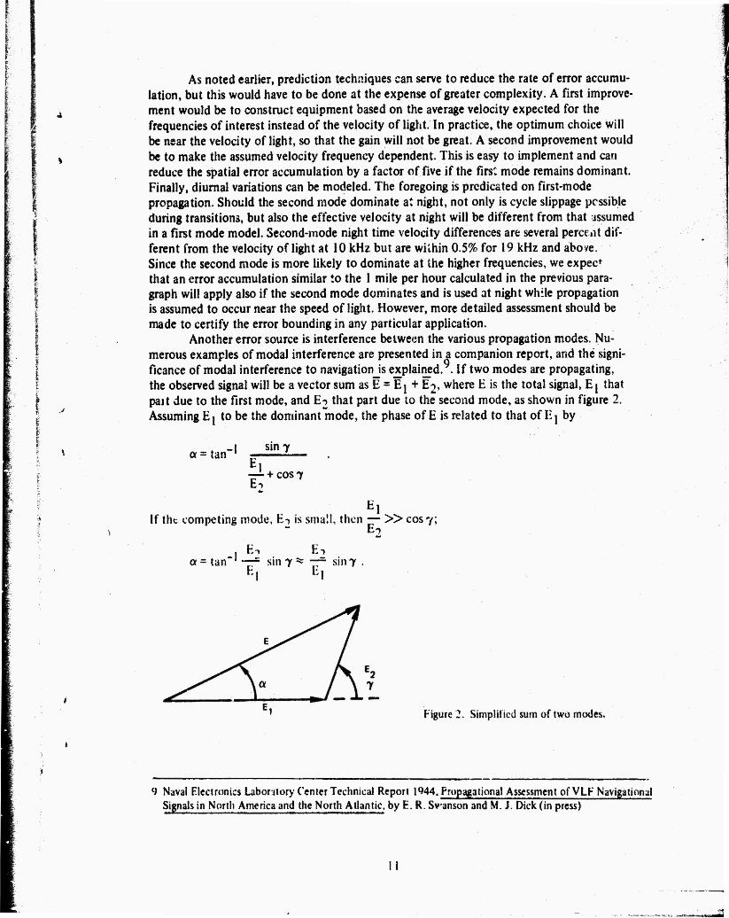
Another error source is interference between the various propagation modes. Nu- merous examples of modal interference are presented in a companion report, and the signi- ficance of modal interference to navigation^ explained. . If two modes are propagating, the observed signal will be a vector sum as E = E j + E2, where E is the total signal, E j that pait due to the first mode, and E2 that part due to the second mode, as shown in figure 2. Assuming Ej to be the dominant mode, the phase of E is related to that of E j by

a = tan" sin 7

El 7-U cos 7 E->

El If tht competing mode, E-> is small, then —- » cos 7;

> " E2 , E-» Ei

a * tan**' *—"" sin 7 "* rf sin 7 • fci Ei

Figure 2. Simplified sum of two modes.

9 Naval Electronics Laboratory Center Technical Report 1944. Propagational Assessment of VLF Navigational Signals in North America and the North Atlantic, by E. R. Svansor» and M. J. Dick (in press)

II

To the degree that the attenuation rates of the two modes are constant in a local region, the resultant phaie perturbation is seen to be a sinusoidal function of propagation path length. Fror.i the viewpoint of navigational safety, the most signifies a feature of the error is that it is bounded, never becoming greater than E7/E j for small perturbations. We now seek the statistical error density distribution resulting from an underlying error structure of this type. Error as a function of propagation path length is assumed sinusoidal as shown in figure 3, Proceeding from first principles, we note that the prubability of an error between certain limits, 6P, is related to the probability density function, f(y), by

i I

OR + 6y

(y1<y<y1+6y)" f f(y)dy.

y\

But since the structure of figure 3 is assumed to exist in various regions and we cannot specily the exact location, X, within a region, we assume aircraft are uniformly distributed in X. Since the errors are symrr "trie, we can further normalize the statistics for an aircraft to be located between Xj and X2 with uniform likelihood. The probability that an aircraft is between any two points Xj and Xj + 5X is thus 5P (Xj < X < X| + 6Xj)■■ 8X1*. But the probability that y is in any particular range is then

5P< (y, <y<yj + 6y)

• -l/yl+6y\ -1 yl

so

OP m /, -1 jyi + 6y| . -lpih r > 6y VTT/ \ / A ( j A \ / ir

K'fl dy »«r:

so

r-i (xM1) ffA \ A /

i\ -Vz (I)

I 0

t z -A

Displacement along propagation path

Figure 3. Model for errors due to modal interference.

12

;-; . ■ '

I I

This probability density function is compared with others of intereri in figure 5 in ERROR SYNTHESIS. It is distinguished by an abnormally high probability of errors near the bound.

Certain instrumental errors may also contribute slightly to the overall error budget. One error source which can ordinarily be neglected with good design is the so-called "5 curve" error. •'' This error dates from the early mechanical phase shifters and »esolvers wherein the resulting shaft angle would not correspond directly to the input phase but would vary slightly as a function of rotation. Modern circuits have an error of much the same type, since engineering embodiments contain a certain inevitable coupling between signals carrying reference phase values and those carrying intelligence. Since the resultant will have a distortion depending on the relative phasing, the actual error will vary from time to time depending on internal references which vary. The essential character of the error is that expressed by eq (1), although individual errors on particular receivers may not appear particularly sint^oidal. Since S-curve errors will ordinarily be small, any reasonable allow- ance for errors due to modal interference will d ninate.

Another instrumental error is that of phase shift with signal amplitude. Proper de- sign can make this error negligible with respect to those being considered herein. The error will tend to resemble a simple bias but may vary as signal amplitudes vary.

If the signals are weak, electromagnetic interference generated aboard the aircraft, thunderstorm-induced radio-frequency noise, and discharge static generated by the aircraft may also be important. Unless interference is coherent and sufficiently narrowband to capture the receive!, or beat with the vlf signals, the effect will be similar to that of normal electromagnetic noise. If noise is small compared with signal, then the resulting phase per- turbations will follow the Gaussian distribution. Theory indicates chat, if the measurements

L are compared against a fixed reference, and therefore a fixed folding function, then, as the signai-to-noise ratio deteriorates, the distribution shifts from Gaussian through cosinusoidal

( to uniform between -# and +* with respect to the reference. In practice, there will also be degradation of the folding criterion and possible loss o*" track. The theoretical bounding is thus more apparent than real. Further, it is to be expected that various individual phase measuivments will be further combined in subsequent tracking filters so that, by the central limit theory, it will be realistic to consider the resultant phase perturbation statistics as Gaussian.

PILOTAGE ERRORS

Actual pilot performances have never been studied precisely. S.*eh a study would be difficult because it w^uld have to be made without the pilot's knowledge. Also, pilotage error from one type of navigation system will not be the same as pilotage error from another, since human error is a function of the navigation system used. However, experienced

10 Naval Electronics Laboratory Center Technical Note 1529, Accuracy Tests on Tracor 3-499R Omega Receivers, by J. E. Britt, 21 August 1969 (NELC TNs are informal documents intended chiefly for use within NELC)

! 1 Swan son, E. R., Gimber, R. H., and Britt, J. E., "Calibrated VLF Phase Measurements: Simultaneous Remote and Local Measurements of 10.2 kHz Carrier Phase Using Cesium Standaras," Proc 4th Ann DoD Precise Time and Time Interval (PTT1) Strat Plan Mtg, 14-16 November 1972, p. 232-248

12 National Aviation Facilities Experimental Center Report No. RD-65-98, VOR System Accuracy, by N. Braverman, E. Laskowski, and 0. DcsRosier, August 1965 ~

13

>«^yJBIMIt.|M4!U4i!!l".>-1-1---1 -■■- ~~~ ' "~^"

personnel of the Flight Standards Service have made estimates of pilotage error for VOR navigation. 12 While this will differ from vlf pilotage error, perhaps the estimate will pro- vide a rough prediction of the pilotage error expected from vlf navigation.

The Flight Standards Service estimates that the two-standard-deviation (95% proba- bility) VOR pilotage error is 2.5° without autopilot, 1° with autopilot, and 1.8° with auto- pilot in the heading mode; thus, one-standard-deviation error without autopilot would be 2.5°/2 = 1.25°. With VOR, this error corresponds to 1/2 mile it a range of 23 miles and less at shorter ranges, increasing to 1.25 miles at 60 miles. This error, however, can be con- sidered composed of two components. One inherent component is that associated with the ability to fly a given aircraft on a desired course. The second is that associated with the ability to read the VOR needle, which covers a range of ±45°. A deflection indicating 1.25° is relatively small, and some significant part of the deduced pilotage error may be due to the scale chosen for the VOR display. A convenient scale for vlf lateral track error and one used commercially is for deviations of approximately ±2 nmi in nearly the same size and display configuration used with VOR. if the pilotage error deduced in the Flight Standards estimate was entirely due to inability to read the VOR needle, then the vlf pilotage error can be computed by proportioning the scale sizes in a manner such that 1.25°:45° half de- flection is as vlf pilotage error: 2-nmi half deflection. This procedure results in a vlf pilotage error of 0.06 nmi. Intuitively, we realize that 0.06 nmi is a rather low pilotage error, espe- cially in rough flying weather. However, personnel familiar with flying by existing vlf equipment have suggested that a pilotage error of the order of 0.1 nmi or less might be typical under favorable flying conditions. Although 0.1 nmi may appear a good estimate for typical pilotage error, a more conservative 1/4 nmi is assumed in following computations.

ACCURACY CRITERION

A design criterion suggested by Braverman has already been noted wherein five standard deviations of the aircraft positioning capability is equated to the traffic separa- tion. ' ** Implied in the criterion is the use of normal statistics. The collision probability can be assessed in two ways from the error distributions shown in figure 4. Consider two aircraft traveling at the same altitude, each of which has a lateral track error given by the normal distribution with variance o^ but in one case centered at -1 /2 s and in the other at 1/2 s, where s is traffic separation. That is. the respective positional distributions are given by NC-l/2 s, cr) and N (1/2 s, o~). The difference between two quantities each of which is normally distributed is also normally distributed but with average equal to the mean

Figure 4. Development of collision risk.

-1/2 S 1/2 S

14

wmam

difference and with variance equal to the sum of the individual variances; that is: N (s, Ion. If no evasive maneuver takes place, then the probability of collision is proportional to the probability that their separation distance is less than some critical distance» b, roughly equal to one-half the sum of widths of the aircraft. Thus, the probability of collision is propor- tional to 13

b b

/N(s,2o2)dx= / _!— -b -b ^V**

exp \4o2/ oyfiT \4o2/

(2)

where we have made use of the fact that b is very small with respect to x and o. The actual collision frequency will also be proportional to the square of the traffic density and to the relative velocity between aircraft. To assess safety of airway structures in which the density, aircraft velocities, and aircraft sizes are much the same, we thus note that the error statistics and structure are fully embodied in (I/o) exp (-s2/4o2) provided the inherent errors are normally distributed.

An alternative formulation is possible wherein normally distributed errors need not be assumed. The problem with the preceding formulation is that, if the distributions of lateral track errors are not normal, then the distribution of the separation distances is not known in advance. More generally, we note that the collision probability will be propor- tional to the sum of the probabilities that one aircraft is at all positions while simultaneously the second aircraft is within ±b of the same locations:

+b

,-b (3)

where f j an J tS are the respective probability density functions. If the error distributions happen to be normal, then

Pa / s-<x+l/2s)2/2o2

sPUta

+b t J_ e-<*-'/2sW2o2dxdx.

Since b is smail,

OO , -I

Pa f JL e^x+l/2s)2/2o2 JL- e-(x-l/2s)2/2a2 dx

a exp <h/JT W (h/¥ S ~-or/a~ dx |

13 Levine, P. H., Adrian, D. J., and Swanson, E. R., "Navigation Accuracy and Maritime Safety," Proc, of the Radio Navigation Symposium, Washington DC, 13-15 November 1973, p. 227-233

15

umpppp BBBjEiifppüggs»! ^^m^p^^im'wm^1^^^'^^^ «?^»y

When the substitution z =y/T\ is made, the quantity in braces is recognized as the complete integral of the normal distribution function and is therefore equal to unity. Thus, if the statistics are normal, eq (3) is equivalent to eq (2), as expected. However, eq (3) is applicable to any statistical distribution and can be readily evaluated by numeric methods to compare navigational risks. More convenient will be a reference probability coefficient,

oo

K= y*f,f2dx, (4)

which is defined to absorb the aircraft size. It is equivalent to defining

P<*2bK. (5)

Airway structures with the same K will be equally safe if carrying the same load. In the case of normally distributed errors,

K.-i-e 2(Vff

■'# 2 -s*7xo** (6)

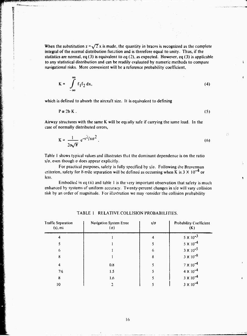
Table 1 shows typical values and illustrates that the dominant dependence is on the ratio s/o, even though o does appear explicitly.

For practical purposes, safety is fully specified by s/o. Following the Braverman criterion, safety for 8-mile separation will be defined as occurring when K is 3 X 10""4 or less.

Embodied in eq (6) and table 1 is the very important observation that safety is much enhanced by systems of uniform accuracy. Twenty-percent changes in s/o will vary collision risk by an order of magnitude. For illustration we may consider the collision probability

TABLE 1 RELATIVE COLLISION PROBABILITIES.

Traffic Separation (s), mi

Navigation System Error (o)

s/o Probability Coefficient (K)

4 1 4 5 X 10"3

5 1 5 5X 10"4

6 1 6 3X 10~5

8 1 8 3 X 10"8

4 0.8 5 7X 10"4

VA 1.5 5 4X 10"4

8 1.6 5 3 X 10"4

10 2 5 3X 10*"4

16

ipllgpllllppp^^

coefficient, K, for an idealized VOR system in which there is perfect accuracy over the VOR and a uniformly degrading accuracy according to range, r. Assume a uniform traffic separa- tion of 8 miles and VOR accuracy degrading to 4.5 miles (two standard deviations) at 60- mile range. The average navigational accuracy (one standard deviation) is 4.5/4 = 1.125 miles and the K associated is 8 X 10 . However, the average K is

TT--L 'max

rmax T .

0J LW* e-s

2/4o(r)2 dr

T.-L f K 60 / p-8

2/4[0.0375rl 5 2[0.0375rlV?

dr,

which is 9 X 10""4 by numeric integration; that is, three orders of magnitude worse than the collision probability associated with the average accuracy. Indeed, in this example the average collision probability is only reached at about the upper pen tile in terms of errors varying with range.

A second criterion for safety has been proposed by Litchford; namely, that a new system need be no more accurate than the existing VOR system. De facto the safety of the VOR system has been accepted for years. Since the computation of the previous para- giaph was typical if idealized, the VOR criterion is equivalent to a probability coefficient of 9 X 10"^ instead of 3 X 10~^ by the Braverman criterion. Considering the sensitivity of the parameters, the two criteria are thus seen to be essentially the same. Safe navigation can be taken as occurring whenever K is about 6 X 10~^ or less.

ERROR SYNTHESIS

The problem of determining proper structure and accuracy for vif iiavigational im- plementations can now be solved by addressing two separate tasks. First, it is necessary to synthesize the various error sources including those peculiar to vlf and also pilotage to de- termine the probability density function. This is properly accomplished by performing a convolution of the various error functions. Second, once the synthesized probability den- sity functions are obtained, it is necessary to place these into eq (4) to obtain the relative collision probabilities. Of special interest is the postulated vlf error structure, wnich, when synthesized with all other errors, yield, a relative collision probability between 3 and 9 X 10""4 and thus provides a satisfactory »evel of safety.

Figure 5 shows the convolution of navigational position fixing error with pilotage error. In each case the pilotage error has been assumed Gaussian with standard deviation 1/4 nmi. This is believed a conservative assumption as discussev! on page 13. The naviga- tional position fixing errors have all been depicted to exhibit the -ame scatter, o = 1-1/2 nmi. The navigation aid and pilotage errors have been chosen as rounded-off values which will yield safe conditions when synthesized with Gaussian errors. The only variable in figure 5 is the shape of the distribution of navigational position fixing errors. In addition

14 Litchford, G., Analyst! of Ait Traffic Control Safety Using VLF Signals, Litchford Systems Incorporated Report under NELC N0M5J-744I-243Z. April 1974

17

TOgpypf^^^ällftlJIJU^!^

Navigation«) Position C". »ed Fixing Error nh\

0 = 1.5 nmi

Pilotage Error

O « 0.25 nmi

Yields Total Navigation Error

a - 1.62 nmi

1.6

f(Y) ,

1.6

1-6 I \ f(Y)

f(Y) 0.19

f(Y>

0 2.6 Uniform

3.0

0 2.1

d<Sin"1»

Figure 5. Error convolutions.

18

■Pf l«Lyjl„WL.LWll,i4^l!UllJJ.i|.|lillJI iPPWMPWPPPqP^jy - -■ - - *?-=■

to Gaussian shown for reference, the triangular and unitorm distributions are shown v dis- cussed on page 10, figure 1, and the differential arc sine is shown as derived on page I2,eq(l). The distribution functions are all mathematically idealized but represent conceivable tend- encies . As discussed earlier, the Gaussian would arise from the central limit theorem and a number of error sources. The triangular or uniform function could arise from initialization procedures and reasonable flight scenarios. The differential arc sine will arise if modal inter- ference is a dominant error source. Except for the Gaussian distribution, the errors are especially characteristic of embodiments of vlf aircraft navigation systems and have the common feature that there is some type of a bounding. The convolutions were performed numerically by specially written computer programs.

Figure 6 shows the safety associated with each of the error structures derived \n figure 5. Safety was evaluated in each case by nimeri^ multiplication and integration of the convolutions previously obtained with eq (4). Safe operation will occur when 1he air- ways and navigational aid characteristics are designed so that K <J 6 X 10 , which is ap- proximated in the Gaussian example. (The factor-of-three difference is slight considering the sensitivity of the functions and is due to round-off in choosing the initial standard deviations.) The case of triangularly distributed navigational errors is the least-safe of the vlf-type error distributions but nonetheless 1000 times as safe as the distribution of Gaus- sian errors of the same variance. Most safety would result from a modal interference type error which provides 10"6 times the safety resulting from Gaussian eirors of the same variance. Safety is primarily determined by the bound on the navigational error. The com- putations dramatically emphasize the importance of the nature of the navigational errors in determining safety.

A more significant question is that posed by the inverse problem; that is, determin- ing the error bound permissible by each error distribution which still allows safe operat A.

This computation has been performed by iterative techniques and yields the results of table 2. Most significant is the error bounding for the vlf error models near 4 miles. This reflects the obvious truth that if opposing traffic is restrained to deviate no more than half the separation distance, the aircraft will not collide. What is not obvious is that some minor random Gaussian distributed error as represented by pilotage has very little effect. Indeed, the bound for triangular distributions actually allows some overlap between adjacent traffic lanes. What the computations show is that the hazard associated with the overlap still allows operation within established safety criteria.

Many other distributions could be considered and computations performed to further illuminate the importance of navigational errors to safety. Much woiV needs to be done. However, one additional computation will help to establish present requirements. It is to be expected that some aircraft will continue to be navigated by conventional methods. If these approximate Gaussian error distributions, we then need to consider the collision be- tween aircraft with Gaussian error distributions and those with more typically vlf error dis- tributions. One such calculation has been performed wherein the Gaussian errors were as- sumed to have standard deviation of l .7 nmi as typical of present VOR navigation at 40 miles and the vlf errors were assumed uniform. * * Safe operation was found tc occur when the uniform distribution was bounded at 3.5 nmi (standard deviation of 2.1 nmi).

The foregoing analysis indicates that 8-mile-separation airways will be adequately safe if the prevailing navigational fixing system is designed IO bound an error to 3.5-4.4 nmi, depending on the distribution of the respective prevailing errors.

19

Total Navigational Error Probability Dantitits

Safety Ralatiwt Probability Coefficient

(K)

2X tO-4

0X1O-7

0.19

L MY)

0.19

XL f(Y)

A 3.0 3.0

6X 10 r19

2.1 ° 2.1 2.1 0 2.1

SX 10 r29

Figure 6. Safely associated with various error structures (sale operation occurs when K <6 X I0"4).

20

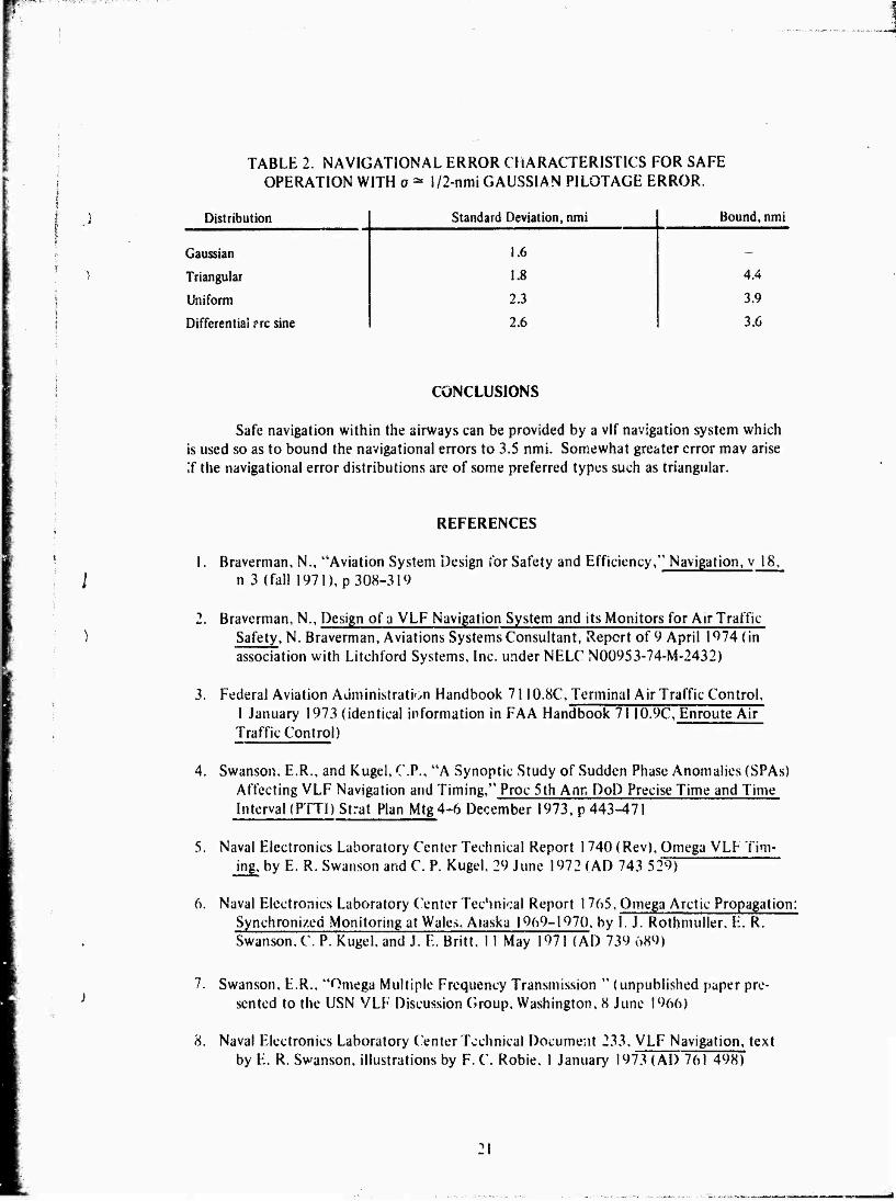
TABLE 2. NAVIGATIONAL ERROR CHARACTERISTICS FOR SAFE OPERATION WITH o Ä 1/2-nmi GAUSSIAN PILOTAGE ERROR.

Distribution Standard Deviation, nmi Bound, nmi

Gaussian 1.6 _

Triangular 1.8 4.4

Uniform 2.3 3.9

Differential ?rc sine 2.6 3.C

CONCLUSIONS

Safe navigation within the airways can be provided by a vlf navigation system which is used so as to bound the navigational errors to 3.5 nmi. Somewhat greater error mav arise if the navigational error distributions are of some preferred types such as triangular.

REFERENCES

1. Braverman, N., "Aviation System Design for Safety and Efficiency," Navigation, v 18, n 3 (fall 1971), p 308-319

2. Braverman, N., Design of a VLF Navigation System and its Monitors for Air Traffic- Safety, N. Braverman, Aviations Systems Consultant, Report of 9 April 1974 (in association with Litchford Systems, Inc. under NELC N00953-74-M-2432)

3. Federal Aviation Administration Handbook 7110.8C, Terminal Air Traffic Control, 1 January 1973 (identical information in FAA Handbook 7110.9C, Enroute Air Traffic Control)

4. Swanson, E.R., and Kugel, C.P., "A Synoptic Study of Sudden Phase Anomalies (SPAs) Affecting VLF Navigation and Timing," Proc 5th Ann DoD Precise Time and Time Interval (PTTI) Strat Plan Mtg4-6 December 1973, p 443-471

5. Naval Electronics Laboratory Center Technical Report 1740 (Rev), Omega VLF Tim- ing, by E. R. Swanson and C. P. Kugel, 29 June 1972 (AD 743 529)

6. Naval Electronics Laboratory Center Technical Report 1765, Omega Arctic Propagation: Synchronized Monitoring at Wales, Alaska 1969-1970, by I. J. Rothmuller, E. R. Swanson, C P. Kugel, and J. E. Britt, 11 May 1971 (AD 739 689)

7. Swanson. E.R., "Omega Multiple Frequency Transmission " (unpublished paper pre- sented to the USN VLF Discussion Group, Washington, 8 June 1966)

8. Naval Electronics Laboratory Center Technical Document 233, VLF Navigation, text by E. R. Swanson, illustrations by F. C. Robie. I January 1973 (AD 761 498)

9. Naval Electronics Laboratory Center Technical Report 1944, Propagaiional Assessment of VLF Navigation*»1 cignals in North America and the North Atlantic, by E. R. Swanson and M. J. Dick (in press)

10. Naval Electronic Laboratory Center Technical Note 1529, Accuracy Tests on Tracor 3-499R Omega Receivers, by J. E. Britt, 21 August 1969*

11. Swanson, E.R., Gimber, R.H., and Briti, J.E., "Calibrated VLF Phase Measurements: Simultaneous Remote and Local Measurements of 10.2 kHz Carrier Pht.se Using Cesium Standards," Proc 4th Ann DoP Precise Time and Time Interval (PTT1) Strat Plan Mtg, 14-16 November 1972, p 232-248

12. National Aviation Facilities Experimental Center Report No. RD-65-98, VOR System Accuracy, by N. Braverman, E. Laskowski, and O. DesRosier, August 1965

13. Levine, P. H., Adrian» D. J., and Swanson, E. R., "Navigation Accuracy and Maritime Safety,1' Proc of the Radio Navigation Symposium, Washington DC, 13-15 Novem- ber 1973,p 227-233

14. Litchford, G., Analysis of Air Traffic Control Safety Using VLF Signals, Litchford Systems Incorporated Report under NELC N00953-74-M-2432, April 1974

*NELC TNs are informal documents intended chiefly for use within NELC.