Design and Analysis of Multi-Factored Experimentsllye/DOE course - Part 12a - RSM.pdf · Design and Analysis of Multi-Factored Experiments Response Surface Methodology (RSM) L . M

1

Design and Analysis of Multi-Factored Experiments

Response Surface Methodology (RSM)

L . M. Lye DOE Course 1

(RSM)

Introduction to Response Surface Methodology (RSM)

• Best and most comprehensive reference:• Best and most comprehensive reference:– R. H. Myers, D. C. Montgomery and C. M. A. Cook

(2009): Response Surface Methodology: Process and Product Optimization Using Designed Experiments, John Wiley and Sons.

• Best software:


– Design-Expert Version 8, Statease Inc.– Available at www.statease.com– Minitab also has DOE and RSM capabilities

2

RSM: Introduction

• Primary focus of previous discussions is factorscreening– Two-level factorials, fractional factorials are widely

used• RSM dates from the 1950s (Box and Wilson,

1951)• Early applications in the chemical industry


• Currently RSM is widely used in quality improvement, product design, uncertainty analysis, etc.

Objective of RSM• RSM is a collection of mathematical and statistical

techniques that are useful for modeling and analysis in applications where a response of interest is influenced by several variables and the objective is to optimize the response.

• Optimize maximize, minimize, or getting to a target.


target.• Or, where a nonlinear model is warranted when

there is significant curvature in the response surface.

3

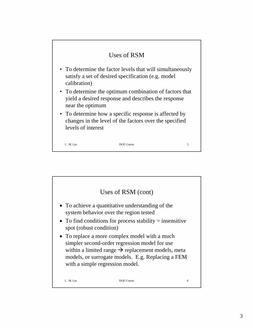
Uses of RSM

• To determine the factor levels that will simultaneously satisfy a set of desired specification (e g modelsatisfy a set of desired specification (e.g. model calibration)

• To determine the optimum combination of factors that yield a desired response and describes the response near the optimum

• To determine how a specific response is affected by


To determine how a specific response is affected by changes in the level of the factors over the specified levels of interest

Uses of RSM (cont)

• To achieve a quantitative understanding of the system behavior over the region testedsystem behavior over the region tested

• To find conditions for process stability = insensitive spot (robust condition)

• To replace a more complex model with a much simpler second-order regression model for use within a limited range replacement models meta


within a limited range replacement models, meta models, or surrogate models. E.g. Replacing a FEM with a simple regression model.

4

ExampleSuppose that an engineer wishes to find the levels of temperature (x1) and feed concentration (x2) that maximize the yield (y) of a process. The yield is a y (y) p yfunction of the levels of x1 and x2, by an equation:

Y = f (x1, x2) + ε

If we denote the expected response by


E(Y) = f (x1, x2) = η

then the surface represented by:

η = f (x1, x2)

is called a response surface.

The response surface maybe represented graphically using a contour plot and/or a 3-D plot.


In the contour plot, lines of constant response (y) are drawn in the x1, x2, plane.

5


These plots are of course possible only when we have two factors.

With more than two factors the optimal yield hasWith more than two factors, the optimal yield has to be obtained using numerical optimization methods.

In most RSM problems, the form of the relationship between the response and the


p pindependent variables is unknown. Thus, the first step in RSM is to find a suitable approximation for the true relationship between Y and the X’s.

6

If the response is well modeled by a linear function of the independent variables, then the approximating function is the first-order model (linear):

Y = β0 + β1 x1 + β2 x2 + … + βk xk + ε

This model can be obtained from a 2k or 2k-p design.

If there is curvature in the system, then a polynomial of higher degree must be used, such as the second-order model:


Y = β0 + Σβi xi + Σβii x2i + ΣΣβij xi xj + ε

This model has linear + interaction + quadratic terms.

• Many RSM problems utilize one or both of these approximating polynomials. The response surface analysis is then done in terms of the fitted surface. yThe 2nd order model is nearly always adequate if the surface is “smooth”.

• If the fitted surface is an adequate approximation (high R2) of the true response function, then analysis of the fitted surface will be approximately


equivalent to analysis of the actual system (within bounds).

7

Types of functions

• Figures 1a through 1c on the f ll i ill iblfollowing pages illustrate possible behaviors of responses as functions of factor settings. In each case, assume the value of the response increases from the bottom of the figure to the top


from the bottom of the figure to the top and that the factor settings increase from left to right.

Types of functions


Figure 1a

Linear function

Figure 1b

Quadratic function

Figure 1c

Cubic function

8

• If a response behaves as in Figure 1a, the design matrix to quantify that behavior need only contain factors with two levels -- low and high.

• This model is a basic assumption of simple two-level factorial and fractional factorial designs.

• If a response behaves as in Figure 1b, the minimum number of levels required for a


minimum number of levels required for a factor to quantify that behavior is three.

• One might logically assume that adding center points to a two-level design would satisfy that requirement, but the arrangement of the treatments in such a matrix confounds all quadratic effects with each other.

• While a two level design with center points cannot• While a two-level design with center points cannot estimate individual pure quadratic effects, it can detect them effectively.

• A solution to creating a design matrix that permits the estimation of simple curvature as shown in Figure 1b would be to use a three-level factorial design. Table 1 explores that possibility.


explores that possibility.• Finally, in more complex cases such as illustrated in

Figure 1c, the design matrix must contain at least four levels of each factor to characterize the behavior of the response adequately.

9

Table 1: 3 level factorial designs

• No. of factors # of combinations(3k) Number of coefficients• 2 9 6• 3 27 103 27 10• 4 81 15• 5 243 21• 6 729 28

• The number of runs required for a 3k factorial becomes unacceptable even more quickly than for 2k d i


2k designs. • The last column in Table 1 shows the number of

terms present in a quadratic model for each case.

Problems with 3 level factorial designs

• With only a modest number of factors, the number of runs is very large, even an order of magnitude

t th th b f t t bgreater than the number of parameters to be estimated when k isn't small.

• For example, the absolute minimum number of runs required to estimate all the terms present in a four-factor quadratic model is 15: the intercept term, 4 main effects, 6 two-factor interactions, and


4 quadratic terms. • The corresponding 3k design for k = 4 requires 81

runs.

10

• Considering a fractional factorial at three levels is a logical step, given the success of fractional designs when applied to two-level designs.

• Unfortunately, the alias structure for the three-level fractional factorial designs is considerably more complex and harder to define than in the two-level case.

• Additionally, the three-level factorial designs


suffer a major flaw in their lack of `rotatability’• More on ‘rotatability’ later.

Sequential Nature of RSM• Before going on to economical designs to fit second-

order models, let’s look at how RSM is carried out in general.

• RSM is usually a sequential procedure. That is, it done in small steps to locate the optimum point, if that’s the objective. This is not always the only objective.


• The analogy of climbing a hill is appropriate here (especially if it is a very foggy day)!

11

Sequential Nature of RSM (continue)• When we are far from the optimum (far from the

peak) there is little curvature in the system (slight p ) y ( gslope only), then first-order model will be appropriate.

• The objective is to lead the experimenter rapidly and efficiently to the general vicinity of the optimum.

• Once the region of the optimum has been found a


• Once the region of the optimum has been found, a more elaborate model such a second-order model may be employed, and an analysis performed to locate the optimum.


12

• The eventual objective of RSM is to determine the optimum operating conditions for the system or to determine a region of the factor space in which

i ifi i i fi doperating specifications are satisfied. • The word “Optimum” in RSM is used in a special

sense. The “hill climbing” procedures of RSM guarantee convergence to a local optimum only.

• In terms of experimental designs, when we are far f i i l 2k f i l i


from optimum, a simple 2k factorial experiment would allow us to fit a first-order model. As we get nearer to the peak, we can check for curvature by adding center-points to the 2k factorial.

• If curvature is significant, we may now be in the vicinity of the peak and we use a more elaborate design (e.g. a CCD) to fit a second-order model to “capture” the optimum.


13

Method of Steepest Ascent• The method of steepest ascent is a procedure for

moving sequentially along the path of steepest ascent (PSA), that is, in the direction of the ( ), ,maximum increase in the response. If minimization is desired, then we are talking about the method of steepest descent.

• For a first-order model, the contours of the response surface is a series of parallel lines. The


direction of steepest ascent is the direction in which the response y increases most rapidly. This direction is normal (perpendicular) to the fitted response surface contours.

First-order response and PSA


14

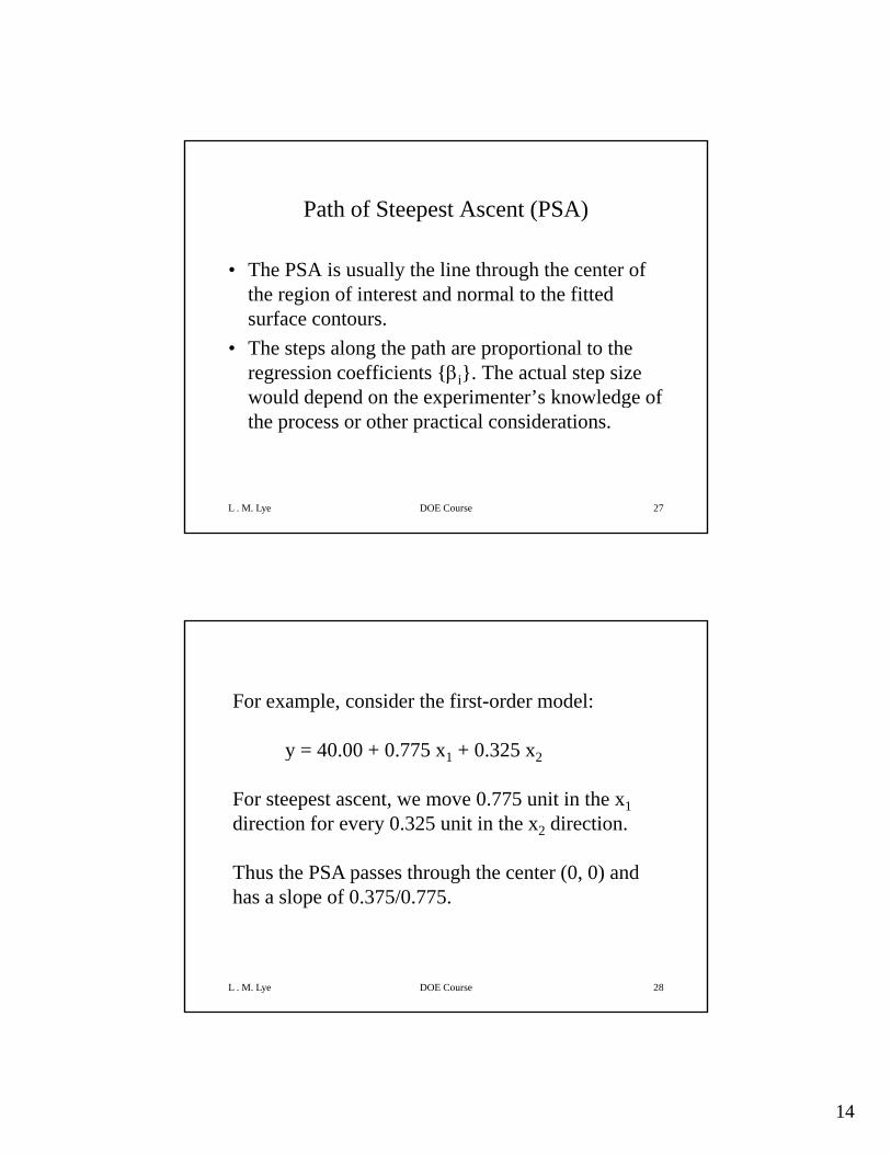
Path of Steepest Ascent (PSA)

• The PSA is usually the line through the center of• The PSA is usually the line through the center of the region of interest and normal to the fitted surface contours.

• The steps along the path are proportional to the regression coefficients {βi}. The actual step size would depend on the experimenter’s knowledge of


would depend on the experimenter s knowledge of the process or other practical considerations.

For example, consider the first-order model:

y = 40 00 + 0 775 x + 0 325 xy = 40.00 + 0.775 x1 + 0.325 x2

For steepest ascent, we move 0.775 unit in the x1direction for every 0.325 unit in the x2 direction.

Thus the PSA passes through the center (0, 0) and


p g ( , )has a slope of 0.375/0.775.

15

If say 1 unit of x1 is actually equal to 5 minutes in actual units, and 1 unit of x2 is actually equal to 5 °F,

the PSA are Δx1 = 1.00 and

Δx2 = (0.375/0.775) Δx2 = 0.42 = 2.1 °F.

Th f ill l th PSA b


Therefore, you will move along the PSA by increasing time by 5 minutes and temperature by 2 °F. An actual observation on yield will be determined at each point.

• Experiments are then conducted along the PSA until no further increase in the response is

b dobserved. • Then a new first-order model may be fit, a new

direction of steepest ascent determined, and further experiments conducted in that direction until the experimenter feels that the process is near the optim m (peak of hill is ithin grasp!)


the optimum (peak of hill is within grasp!).

16


Yield vs steps along the PSA

• The steepest ascent would terminate after about 10 steps with an observed response of about 80%. Now we move on to the next step.Now we move on to the next step.

• Fit another first-order model with a new center (where step 10 is) and check whether there is a new PSA.

• Repeat until peak is near. • See flowchart on the next slide


• See flowchart on the next slide.

17

L . M. Lye DOE Course 33Flowchart for RSM

Steps in RSM• Fit linear model/planar models using two-level

factorials• From results, determine PSA (Descent)• Move along path until no improvement occurs• Repeat steps 1 and 2 until near optimal (change of

direction is possible)• Fit quadratic model near optimal in order to


q pdetermine curvature and find peak. This phase is often called “method of local exploration”

• Run confirmatory tests

18

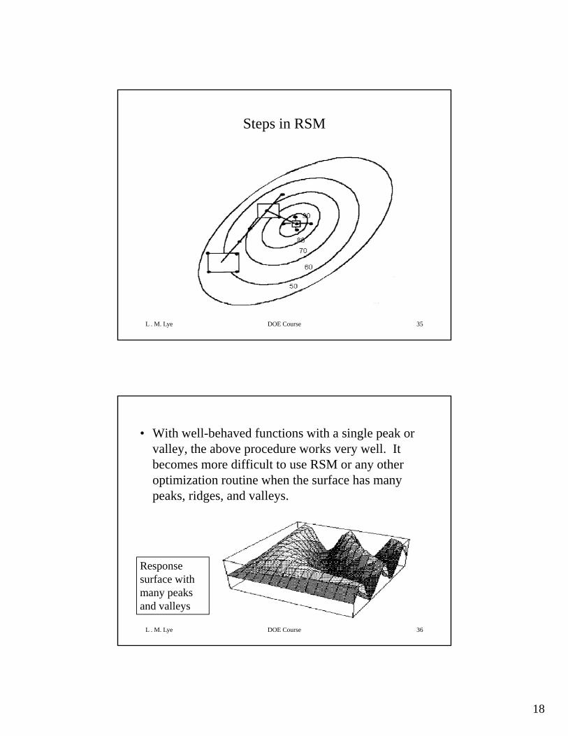
Steps in RSM


• With well-behaved functions with a single peak or valley, the above procedure works very well. It becomes more difficult to use RSM or any other optimization routine when the surface has manyoptimization routine when the surface has many peaks, ridges, and valleys.

R


Response surface with many peaks and valleys

19

Multiple Objectives

• With more than 2 factors, it is more difficult to determine where the optimal is. There may be several possible “optimal” points and not all are desirable. Whatever the final choice of optimal factor levels, common sense and process knowledge must be your guide.

• It is also possible to have more than one response i bl ith diff t bj ti ( ti


variable with different objectives (sometimes conflicting). For these cases, a weighting system may be used to for the various objectives.

Methods of Local Exploration

• The method of steepest ascent, in addition to fitting first order model must provide additionalfitting first-order model, must provide additional information that will eventually identify when the first-order model is no longer valid.

• This information can come only from additional degrees of freedom which are used to measure “lack of fit” in some way


lack of fit in some way. • This means additional levels and extra data points.• It is rare to go more than 5 levels for even the

most complex response surfaces.

20

Consider the 2nd order model:

Y β + β + β + + βY = β0 + β1 x1 + β2 x2 + … + βk xk+ β11 x1

2 + β22 x22 + … + βkk xk

2

+ β12 x1 x2 + … + β1k x1 xk + … + β23 x2 x3+ … + βk-1,k xk-1 xk + ε ------- EQN (1)

To be able to fit a 2nd order model like EQN (1),


To be able to fit a 2 order model like EQN (1), there must be least three levels and enough data points.

Designs for fitting 2nd order models

• Two very useful and popular experimental designs• Two very useful and popular experimental designs that allow a 2nd order model to be fit are the:

• Central Composite Design (CCD)• Box-Behnken Design (BBD)


• Both designs are built up from simple factorial or fractional factorial designs.

21

3-D views of CCD and BBD


Central Composite Design (CCD)

• Each factor varies over five levels• Each factor varies over five levels • Typically smaller than Box-Behnken designs • Built upon two-level factorials or fractional

factorials of Resolution V or greater• Can be done in stages factorial + centerpoints +

i l i t


axial points• Rotatable

22

General Structure of CCD• 2k Factorial + 2k Star or axial points + nc

CenterpointsCenterpoints • The factorial part can be a fractional factorial as

long as it is of Resolution V or greater so that the 2 factor interaction terms are not aliased with other 2 factor interaction terms.

• The “star” or “axial” points in conjunction with


• The star or axial points in conjunction with the factorial and centerpoints allows the quadratic terms (βii) to be estimated.

Generation of a CCD

Factorial Axialpoints +

centerpoints

Axial points


23

Axial points are points on the coordinate axes at distances “α”from the design center; that is, with coordinates: For 3factors, we have 2k = 6 axial points like so:

(+α 0 0) ( α 0 0) (0 +α 0) (0 α 0) (0 0 +α)(+α, 0, 0), (-α, 0, 0), (0, +α, 0), (0, -α, 0), (0, 0, +α),(0, 0, -α)

The “α” value is usually chosen so that the CCD is rotatable.

At least one point must be at the design center (0, 0,0) Usually more than one to get an estimate of “pure


0). Usually more than one to get an estimate of pureerror”. See earlier 3-D figure.

If the “α” value is 1.0, then we have a face-centered CCD Not rotatable but easier to work with.

A 3-Factor CCD with 1 centerpointA 3 factor CCD with nc=1

Runs x1 x2 x3

1 -1 -1 -123456789

10

1-11-11-11

-1.6821.682

-111-1-11100

-1-1-1111100


1112131415

00000

-1.6821.682

000

00

-1.6821.682

0

24

Values of α for CCD to be rotatable

k=2 3 4 5 6 7

1.414 1.682 2.000 2.378 2.828 3.364

The α value is calculated as the 4th root of 2k.


For a rotatable design the variance of the predicted response is constant at all points that

are equidistant from the center of the design

Types of CCDs

The diagrams illustrate the three types of central composite designs for two factors. Note that the CCC explores the largest process space and the CCI explores the smallest process space. Both the CCC and CCI are rotatable designs, but the CCF is not. In the CCC design, the design points describe a circle

b d b h f i l


circumscribed about the factorial square. For three factors, the CCC design points describe a sphere around the factorial cube.

25

Box-Behnken Designs (BBD)• The Box-Behnken design is an independent

quadratic design in that it does not contain an b dd d f t i l f ti l f t i l d iembedded factorial or fractional factorial design.

• In this design the treatment combinations are at the midpoints of edges of the process space and at the center.

• These designs are rotatable (or near rotatable) and require 3 levels of each factor.


require 3 levels of each factor. • The designs have limited capability for orthogonal

blocking compared to the central composite designs.

BBD - summary

• Each factor is varied over three levels (within low• Each factor is varied over three levels (within low and high value)

• Alternative to central composite designs which requires 5 levels

• BBD not always rotatableC bi ti f 2 l l f t i l d i f th


• Combinations of 2-level factorial designs form the BBD.

26

A 3-Factor BBD with 1 centerpoint A 3-factor BBD with nc=3

Runs x1 x2 x3

1 -1 -1 0

11

23456789

10

-111-1-11100

1-110000-1-1

000-11-11-11


10111213

0000

1110

1-110

Brief Comparison of CCD and BBD

With one centerpoint, for k = 3, CCD requires 15 runs; BBD requires 13 runsk = 4, CCD requires 25 runs; BBD also requires 25 runsk = 5, CCD requires 43 runs; BBD requires 41 runs

but, for CCD we can run a 25-1 FFD with Resolution V. Hence we need only 27 runs


Hence we need only 27 runs.

In general CCD is preferred over BBD. See separate handout comparing CCD and BBD in more detail.

27

Analysis of the fitted response surface• The fitted response surface can take on many

hshapes. • For 2 or less dimensions, we can plot the response

against the factor(s) and graphically determine where the optimal response is.

• We can also tell from the contour plots or 3-D l h h h i i i


plots whether we have a maximum, minimum, or a saddle point. These points are stationary points.

Types of stationary points


a) Maximum point; b) Minimum point; c) Saddle point

28

With more than 2 factors

• For more than 2 factors, we need to use numerical th d t t ll h t ki d f t ti i tmethods to tell what kind of stationary point we

have. • In some cases, even this fails.• The levels of the k factors at which the response is

optimal can be determined for the unconstrained b i l l l


case by simple calculus.

When k=1Consider the 2nd order prediction model with k =1:

Provided that b2 is not zero, the optimum response is obtained by:

2210ˆ xbxbby ++=

02 21 =+= xbbddy


Giving:

21dx

2

12bbx −=

29

For k > 1

In the case of k > 1, we can write the 2nd order equation

y = b0 + b1 x1 + b2 x2 + … + bk xk+ b11 x1

2 + b22 x22 + … + bkk xk

2

+ b12 x1 x2 + … + b1k x1 xk + … + b23 x2 x3+ … + bk-1,k xk-1 xk

i i i f


in a more convenient matrix form as:

y = b0 + x’ b + x’ B x

⎥⎥⎥⎥⎤

⎢⎢⎢⎢⎡

=bb

M2

1

b

Where:

⎥⎥⎥⎥⎤

⎢⎢⎢⎢⎡

=xx

M2

1

x

⎥⎦

⎢⎣ kb

⎥⎥⎤

⎢⎢⎡

k

k

bbbbbb

L

L

221

221221

121

1221

11

⎥⎦

⎢⎣ kx


⎥⎥⎥⎥

⎦⎢⎢⎢⎢

⎣

=

kkkk

k

bbb L

MMM

221

121

2222122B

30

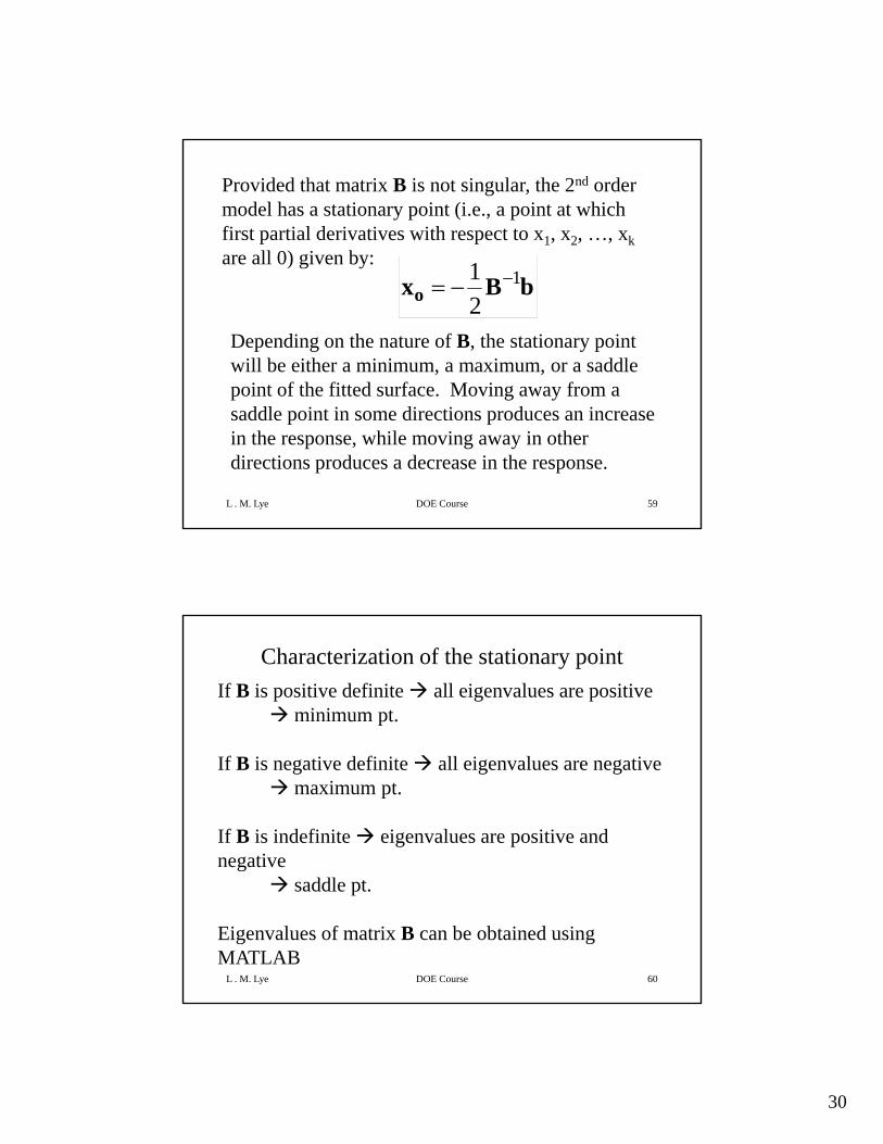
Provided that matrix B is not singular, the 2nd order model has a stationary point (i.e., a point at which first partial derivatives with respect to x1, x2, …, xkare all 0) given by: 1 bBxo

121 −−=

Depending on the nature of B, the stationary point will be either a minimum, a maximum, or a saddle point of the fitted surface. Moving away from a


p g ysaddle point in some directions produces an increase in the response, while moving away in other directions produces a decrease in the response.

Characterization of the stationary pointIf B is positive definite all eigenvalues are positive

minimum pt.

If B is negative definite all eigenvalues are negative maximum pt.

If B is indefinite eigenvalues are positive and negative


saddle pt.

Eigenvalues of matrix B can be obtained using MATLAB

31

Be aware that the xo obtained are random variables and have associated uncertainty with them as are the eigenvalues and matrix B.

There will be situations when an unconstrained optimum will not be useful (when there is a saddle point). We need to consider a constraint that forces us to stay within the experimental region. The procedure that has been developed for this is called ridge


that has been developed for this is called ridge analysis (see Myers and Montgomery). Need to use Lagrange multipliers here for the optimization.

There are also other methods for solving optimization problems constrained or unconstrained th t d t i th t ki f ti l d i tithat do not require the taking of partial derivatives

Direct Optimization procedures. E.g. Nelder-Mead simplex search procedure, or by Monte Carlo simulation.


RSM are now done mainly by software except for simple cases.

32

Other Aspects of Response Surface Methodology• Robust parameter design and process robustness

studies– Find levels of controllable variables that optimize mean

d i i i i bilit i thresponse and minimize variability in the response transmitted from “noise” variables

– Original approaches due to Taguchi (1980s)– Modern approach based on RSM

• Experiments with mixtures– Special type of RSM problem


– Design factors are components (ingredients) of a mixture

– Response depends only on the proportions– Many applications in product formulation

Designs for computer experiments• Much developments of sophisticated engineering

designs, analysis, and products are now carried out by high powered computer simulationsby high-powered computer simulations.

• Some of these sophisticated programs require either expensive computing resources or computer time.

• Hence simplifying the model by means of a meta model or replacement model often makes more


psense. Done properly using DOE methods also helps to understand the complex model a little better.

33

• If the objective is to estimate a polynomial transfer function, traditional RSMs such as CCD and BBD have been used with some success.

• However when analyzing data from computerHowever, when analyzing data from computer simulations, we must keep in mind that the true model will only be approximated by RSM.

• The RSM metamodel will not only fall short in the form of the model, but also in the number of factors.


• Therefore, predictions will only be good within the ranges of the factors specified and will exhibit systematic error, or bias.

• The systematic error is what will be measured in the residual – not the normal variations observed from a random physical process.

• Despite these circumstances much of the standard• Despite these circumstances, much of the standard statistical analyses remain relevant, including model-fit such as the Prediction R2.

• However, the p-values will not be accurate estimates of risks associated with the overall model or any of its specific terms.


• The goal of fitting a RSM to deterministic computer simulated data is for a perfect fit so that there is no systematic error.

34

Check list for quality of fit of designs for RSM• Generate information throughout the region of interest.• Ensure the fitted value be as close as possible to the true value.• Give good detectability of lack of fit.• Allow designs of increasing order to be built up sequentially.• Require a minimum number of runs.• Choose unique design points in excess of the number of

coefficients in the model.• Remain insensitive to influential values and bias from model


Remain insensitive to influential values and bias from model.• Allows one to fit a variety of models.

Newer DOE for Computer Experiments

• Computer models of actual or theoretical physical systems can take many forms and different levels of granularity of representation of the physicalof granularity of representation of the physical system.

• Models are often very complicated and constructed with different levels of fidelity such as the detailed physics-based model as well as more abstract and higher level models with less detailed

i


representation. • A physics-based model may be represented by a

set of equations including linear, nonlinear, ordinary, and partial differential equations.

35

• In view of the complex and nonlinear nature of modern computer models, the classical RSM approaches usually do not provide adequate coverage of the experimental area to provide an accurate metamodel.

• To find a high quality metamodel choosing a good set of• To find a high quality metamodel, choosing a good set of “training” data becomes an important issue for computer simulation.

• Efficient “Space-Filling” designs are able to generate a set of sample points that capture the maximum information between the input-output relationships. E U if D i d L ti h b li t


• E.g. Uniform Designs and Latin hypercube sampling are two such designs.

• http://www.math.hkbu.edu.hk/UniformDesign/

Example of a 20 run, 3 factor, 4 level Uniform Design Uqs (Centered L2)

A B C3 1 1

1 2 3

1 1 3

2 2 4

4 1 2

3 2 2

Levels must be equally spaced.

4 3 4

2 4 1

1 2 1

3 1 4

4 3 1

3 3 3

2 1 2

1 4 2

2 4 4

4 levels allow a cubic equation to be fitted.

Correlations: A, B, C

A BB -0.000

1 000


2 4 4

2 3 1

3 4 3

1 3 4

4 4 2

4 2 3

1.000

C -0.040 0.0000.867 1.000

36

Number of parameters for various models

# FACTORS LINEAR QUADRATIC CUBIC

2 3 6 103 4 10 204 5 15 355 6 21 566 7 28 84


6 7 28 847 8 36 120

N = # of parameters + 4 additional points.

• How to find the best suited metamodel is another key issue in computer experiments.

• Techniques include: kriging models, polynomial regression models, local polynomial regression, multivariate splines and wavelets, and neural networks have been proposed.

• Therefore, design and modelling are two key issues in computer experiments.

• Most of these techniques are outside of statistics although knowledge of classical DOE and RSM


although knowledge of classical DOE and RSM certainly helps in understanding these new techniques.

See papers by Kleijnen et al for more details.

37

12th Annual Golfing Challenge – 3 holes• Conduct an experiment using the golfing toy and

obtain a prediction equation for the toy for use in aobtain a prediction equation for the toy for use in a 3-hole golf championship to be played using the toy in the Faculty Lounge on Saturday, November 17th.

• [Hint: Use a face-centered CCD RS design or BBD RS design]T i h h l l b f k 3


• Team with the least total number of strokes over 3 holes wins 5 extra marks and bragging rights!

• Each team must also summit a report of your experimental design.

Documents

Design and Analysis of Multi-Factored Experimentsllye/DOE course - Part 12a - RSM.pdf · Design and Analysis of Multi-Factored Experiments Response Surface Methodology (RSM) L . M