Embed Size (px)
Citation preview

8/12/2019 Tutorial on Factored Language Models
http://slidepdf.com/reader/full/tutorial-on-factored-language-models 1/39
Factored Language Models Tutorial
Katrin Kirchhoff, Jeff Bilmes, Kevin Duh
{katrin,bilmes,duh}@ee.washington.edu
Dept of EE, University of Washington
Seattle WA, 98195-2500
ElectricalElectrical
EngineeringEngineering
UWUW
UWEE Technical ReportNumber UWEETR-2008-0004February 2008
Department of Electrical EngineeringUniversity of Washington
Box 352500
Seattle, Washington 98195-2500
PHN: (206) 543-2150
FAX: (206) 543-3842
URL: http://www.ee.washington.edu

8/12/2019 Tutorial on Factored Language Models
http://slidepdf.com/reader/full/tutorial-on-factored-language-models 2/39
Factored Language Models Tutorial
Katrin Kirchhoff, Jeff Bilmes, Kevin Duh
{katrin,bilmes,duh}@ee.washington.edu
Dept of EE, University of Washington
Seattle WA, 98195-2500
University of Washington, Dept. of EE, UWEETR-2008-0004
February 2008
Abstract
The Factored Language Model (FLM) is a flexible framework for incorporating various information sources, such
as morphology and part-of-speech, into language modeling. FLMs have so far been successfully applied to tasks
such as speech recognition and machine translation; it has the potential to be used in a wide variety of problems in
estimating probability tables from sparse data.
This tutorial serves as a comprehensive description of FLMs and related algorithms. We document the FLM
functionalities as implemented in the SRI Language Modeling toolkit and provide an introductory walk-throughusing FLMs on an actual dataset. Our goal is to provide an easy-to-understand tutorial and reference for researchers
interested in applying FLMs to their problems.
Overview of the Tutorial
We first describe the factored language model (Section 1) and generalized backoff (Section 2), two complementary
techniques that attempt to improve statistical estimation (i.e., reduce parameter variance) in language models, and that
also attempt to better describe the way in which language (and sequences of words) might be produced.
Researchers familar with the algorithms behind FLMs may skip to Section 3, which describes the FLM programs
and file formats in the publicly-available SRI Language Modeling (SRILM) toolkit.1 Section 4 is a step-by-step walk-
through with several FLM examples on a real language modeling dataset. This may be useful for beginning users of
the FLMs.
Finally, Section 5 discusses the problem of automatically tuning FLM parameters on real datasets and refers to
existing software. This may be of interest to advanced users of FLMs.
1 Introduction to Factored Language Models
1.1 Background
In most standard language models, it is the case that a sentence is viewed as a sequence of T words w1, w2, . . . , wT .
The goal is to produce a probability model over a sentence in some way or another, which can be denoted by
p(w1, w2, . . . , wT ) or more concisely as p(w1:T ) using a matlab-like notation for ranges of words.
It is most often the case that the chain rule of probability is used to factor this joint distribution thus:
p(w1:T ) =t
p(wt|w1:t−1) =t
p(wt|ht)
1This tutorial currently documents the FLM functionalities in SRILM version 1.4.1. Note that while the core FLM functionalities are already
implemented in the SRI language modeling toolkit, additional extensions are still being added. We will update this tutorial to reflect new extensions.
The SRILM toolkit may be downloaded at: http://www.speech.sri.com/projects/srilm/.
1
8/12/2019 Tutorial on Factored Language Models
http://slidepdf.com/reader/full/tutorial-on-factored-language-models 3/39
where ht = w1:t−1. The key goal, therefore, is to produce the set of models p(wt|ht) where wt is the current word
and ht is the multi-word immediately preceding history leading up to word wt. In a standard n-gram based model, it
is assumed that the immediate past (i.e., the preceding n − 1 words) is sufficient to capture the entire history up to the
current word. In particular, conditional independence assumptions about word strings are made in an n-gram model,
where it is assumed that W t⊥⊥W 1:t−n|W t−n+1:t−1. In a trigram (n = 3) model, for example, the goal is to produce
conditional probability representations of the form p(wt|wt−1, wt−2).
Even when n is small (e.g., 2 or 3) the estimation of the conditional probability table (CPT) p(wt|wt−1, wt−2)can be quite difficult. In a standard large-vocabulary continuous speech recognition system there is, for example, a
vocabulary size of at least 60,000 words (and 150,000 words would not be unheard of). The number of entries required
in the CPT would be 60, 0003 ≈ 2 × 10¹⁴ (about 200,000 gigabytes using the quite conservative estimate of one byte
per entry). Such a table would be far to large to obtain low-variance estimates without significantly more trainingdata than is typically available. Even if enough training data was available, the storage of such a large table would be
prohibitive.
Fortunately, a number of solutions have been proposed and utilized in the past. In class-based language models, for
example, words are bundled into classes in order to improve parameter estimation robustness. Words are then assumed
to be conditionally independent of other words given the current word class. Assuming that ct is the class of word wt
at time t, the class-based model can be represented as follows:
p(wt|wt−1) =
ct,ct−1
p(wt|ct) p(ct|ct−1, wt−1) p(ct−1|wt−1)
=
ct,ct−1
p(wt|ct) p(ct|ct−1) p(ct−1|wt−1)
where to get the second equality it is assumed that C t⊥⊥W t−1|C t−1. In order to simplify this further, a number of additional assumptions are made, namely:
1. There is exactly one possible class for each word, or that there is a deterministic mapping (lets say a function
c(·)) from words to classes. This makes it such that p(ct|wt) = δ ct=c(wt), where δ (·) is the Dirac delta function.
It also makes it such that p(wt|ct) = p(wt|c(wt))δ ct=c(wt).
2. A class will contain more than one word. This assumption is in fact what makes class-based language models
easier to estimate.
With the assumptions above, the class-based language model becomes.
p(wt|wt−1) = p(wt|c(wt)) p(c(wt)|c(wt−1))
Other modeling attempts to improve upon the situation given above include particle-based language models [13],
maximum-entropy language models [1], mixture of different-ordered models [9], and the backoff procedure [9, 6], the
last of which is briefly reviewed in Section 2. Many others are surveyed in [9, 6].
1.2 Factored Language Models
In this section, we describe a novel form of model entitled a factored language model or FLM. The FLM was first
introduced in [10, 4] for incorporating various morphological information in Arabic language modeling, but its appli-
cability is more general. In a factored language model, a word is seen as a collection or bundle of K (parallel) factors,
so that wt ≡ {f 1t , f 2t , . . . , f K t }. Factors of a given word can be anything, including morphological classes, stems,
roots, and any other linguistic features that might correspond to or decompose a word. A factor can even be a word
itself, so that the probabilistic language model is over both words and its decompositional factors. While it should be
clear that such a decomposition will be useful for languages that are highly inflected (such as Arabic), the factored
form can be applied to any language. This is because data-driven word-classes or simple word stems or semanticfeatures that occur in any language can be used as factors. Therefore, the factored representation is quite general and
widely applicable.
Once a set of factors for words has been selected, the goal of an FLM is to produce a statistical model over the
individual factors, namely:
p(f 1:K 1:T )
UWEETR-2008-0004 2
8/12/2019 Tutorial on Factored Language Models
http://slidepdf.com/reader/full/tutorial-on-factored-language-models 4/39
or, using an n-gram-like formalism, the goal is to produce accurate models of the form:
p(f 1:K t |f 1:K
t−n+1:t−1)
In this form, it can be seen that an FLM opens up the possibility for many modeling options in addition to those
permitted by a standard n-gram model over words. For example, the chain rule of probability can be used to represent
the above term as follows: k
p(f kt |f 1:k−1t , f 1:K
t−n+1:t−1)
This represents only one possible chain-rule ordering of the factors. Given the number of possible chain-rule orderings
(i.e., the number of factor permutations which is K !) and (approximately) the number of possible options for subsets
of variables to the right of the conditioning bar (i.e., ≈ 2nK ) we can see that an FLM represents a huge family of
statistical language models (approximately K !2nK ). In the simplest of cases, an FLM includes standard n-grams or
standard class-based language models (e.g., choose as one of the factors the word class, ensure that the word variable
depends only on that class, and the class depends only on the previous class). A FLM, however, can do much more
than this.
There are two main issues in forming an FLM. A FLM user must make the following two design decisions:
1. First, choose an appropriate set of factor definitions. This can be done using data-driven techniques or linguistic
knowledge.
2. Second, find the best statistical model over these factors, one that mitigates the statistical estimation difficulties
found in standard language models, and also one that describes the statistical properties of the language in
such a way that word predictions are accurate (i.e., true word strings should be highly probable and any other
highly-probable word strings should have minimal word error).
t M
1t M
−2t M
−3t M
−
t S
1t S −2t
S −3t
S −
t W
1t W
−2t W
−3t W
−
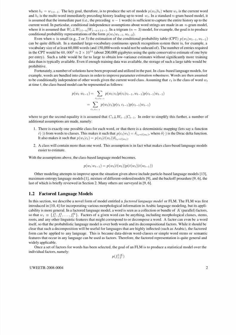
Figure 1: An example of a factored language model seen as a directed graphical model over words W t, morphological
factors W t, and stems S t. The figure shows the dependencies for the variables only at time t for simplicity.
The problem of identifying the best statistical model over a given set of factors can be described as an instance of
the structure learning problem in graphical models [11, 8, 3]. In a directed graphical model the graph depicts a given
probability model. The conditional probability p(A|B, C ) is depicted by a directed graph where there is a node in the
graph for each random variable, and arrows point from B and C (the parents) to A (the child).
We here give several examples of FLMs and the their corresponding graphs. In both examples, only three factors
are used, the word variable at each time W t, the words morphological class M t ( the “morph” as we call it), and the
words stem S t.
The first example corresponds to the following model:
p(wt|st, mt) p(st|mt, wt−1, wt−2) p(mt, wt−1, wt−2)
and is shown in Figure 1. This is an example of a factored class-based language model in that the word class variable
is represented in factored form as a stem S t and morphological class M t. In the ideal case, the word is (almost)
entirely determined by the stem and the morph, so that the model p(wt|st, mt) itself would have very low perplexity
UWEETR-2008-0004 3

8/12/2019 Tutorial on Factored Language Models
http://slidepdf.com/reader/full/tutorial-on-factored-language-models 5/39
(of not much more than unity). It is in the models p(st|mt, wt−1, wt−2) and p(mt, wt−1, wt−2) that prediction (and
uncertainty) becomes apparent. In forming such a model, the goal would be for the product of the perplexities of
the three respective models to be less than the perplexity of the word-only trigram. This might be achievable if it
were the case that the estimation of p(st|mt, wt−1, wt−2) and p(mt, wt−1, wt−2) is inherently easier than that of
p(wt|wt−1, wt−2). It might be because the total number of stems and morphs will each be much less than the total
number of words. In any event, one can see that there are many possiblities for this model. For example, it might be
useful to add M t−1 and S t−1 as additional parents of M t which then might reduce the perplexity of the M t model. In
theory, the addition of parents can only reduce entropy which in term should only reduce perplexity. On the other hand,
it might not do this because the difficulty of the estimation problem (i.e., the dimensionality of the corresponding CPT)
increases with the addition of parents. The goal of finding an appropriate FLM is that of finding the best compromise
between predictability (which reduces model entropy and perplexity) and estimation error. This is a standard problemin statistical inference where bias and variance can be traded for each other.
t M
1t M
−2t M
−3t M
−
t S
1t S −2t
S −3t
S −
t W
1t W
−2t W
−3t W
−
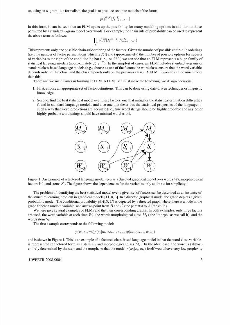
Figure 2: Another example of a factored language model seen as a directed graphical model over words W t, morpho-
logical factors W t, and stems S t. The figure shows the child variable W t and all of its parents. It also shows that the
stem and morph might be (almost) deterministic functions of their parents (in this case the corresponding word) as
dashed lines.
The next example of an FLM is the following:
p(wt|wt−1, wt−2, st−1, st−2, mt−1, mt−2).
This model is similar to the standard word-based trigram but where the two previous stems and morphs have been
added as parents. It is typical that both stems and morphs can be predicted deterministically from the word. I.e., given
a word wt the stem st and the morphological class mt can be determined with certainty2
This model is shown inFigure 2. The word variable W t is shown as the child with parents W t−1, W t−2, S t−1, S t−2, M t−1, M t−2. Also the
deterministic variables are shown with their parents as dashed lines.
There are two interesting issues that become apparent when examining this model. First, the previous morph class
and stem variables are (often) deterministic functions of their parents (previous words). In such a case, therefore, it
should not be useful to use them as additional parents. This is because no additional information can be gleaned from
a new parent if it is only a deterministic function of the set of parents that already exist. For example, given the model
P (A|B, C ) and where D is a deterministic function of C , then the models P (A|B, C ) and P (A|B,C,D) would have
exactly the same entropy.
Even in this case, however, the model above (Figure 2) might have a benefit over a standard word trigram. The
reason is that there might be word trigrams that do not occur in training-data, but the word preceded by the corre-
sponding stems and/or morphs do occur in the same training data set. By using the model in the appropriate way, it
might be detected when a preceding word history does not occur, but the corresponding stem and/or morph history
does occur. This, therefore, would have a benefit in a backoff algorithm over just simply backing-off down to thebigram or unigram (see Section 2.1 for a brief overview of the standard backoff algorithm).
The second interesting issue that arises is the following. When considering just the set of parents in a word trigram
W t−1 and W t−2, and when considering a backoff algorithm, it can reasonably be argued that the best parent to drop
2In some cases, they might not be predictable with certainty, but even then there would be only a small number of different possibilities.
UWEETR-2008-0004 4
8/12/2019 Tutorial on Factored Language Models
http://slidepdf.com/reader/full/tutorial-on-factored-language-models 6/39
first when backing off is the most distant parent W t−2 from the current word W t. This rests on the assumption that the
more distant parent has less predictive power (i.e., ability to reduce perplexity) than does the less distant parent.
On the other hand, when considering a set of parents of a word such as W t−1, W t−2, S t−1, S t−2, M t−1, M t−2, as
shown in Figure 2, it is not immediately obvious nor is there any reasonable a-priori assumption, which can be used to
determine which parent should be dropped when backing off in all cases at all times. In some circumstances, it might
be best to first drop W t−2, but in other cases it might be best to drop W t−1, or perhaps some other parent. In other
words, what backoff order should be chosen in a general model?
The next section addresses both of these issues by introducing the notion we call generalized backoff.
2 Generalized Backoff for FLMs
In this section, we describe the generalized backoff procedure that was initially developed with factored language
models in mind, but turns out to be generally applicable even when using typical word-only based language models
or even when forming arbitrary smoothed conditional probability tables over arbitrary random variables. We will first
briefly review standard backoff in language models, and then present the generalized backoff algorithms.
2.1 Background on Backoff and Smoothing
A common methodology in statistical language model is the idea of backoff . Backoff is used whenever there is
insufficient data to fully estimate a high-order conditional probability table — instead of attempting to estimate the
entire table, only a portion of the table is estimated, and the remainder is constructed from a lower-order model (by
dropping one of the variables on the right of the conditioning bar, e.g., going from a trigram p(wt|wt−1, wt−2) down to
a bigram p(wt|w
t−1)). If the higher-order model was estimated in a maximum-likelihoodsetting, then the probabilities
would simply be equal to the ratio counts of each word string, and there would be no left-over probability for the lower
order model. Therefore, probability mass is essentially “stolen” away from the higher order model and is distributed
to the lower-order model in such a way that the conditional probability table is still valid (i.e., sums to unity). The
procedure is then applied recursively on down to a uniform distribution over the words.
The most general way of presenting the backoff strategy is as follows (we present backoff from a trigram to a
bigram for illustrative purposes, but the same general idea applies between any n-gram and (n − 1)-gram). We are
given a goal distribution p(wt|wt−1, wt−2). The maximum-likelihood estimates of this distribution is:
pML(wt|wt−1, wt−2) = N (wt, wt−1, wt−2)
N (wt−1, wt−2)
where N (wt, wt−1, wt−2) is equal to the number of times (or the count) that the the word string wt−2, wt−1, wt
occurred in training data. We can see from this definition that for all values of wt−1, wt−2, we have that
w
pML(w|wt−1, wt−2) = 1
leading to a valid probability mass function.
In a backoff language model, the higher order distribution is used only when the count of a particular string of
words exceeds some specified threshold. In particular, the trigram is used only when N (wt, wt−1, wt−2) > τ 3 where
τ 3 is some given threshold, often set to 0 but it can be higher depending on the amount of training data that is available.
The procedure to produce a backoff model pBO(wt|wt−1, wt−2) can most simply be described as follows:
pBO(wt|wt−1, wt−2) =
dN (wt,wt−1,wt−2) pML(wt|wt−1, wt−2) if N (wt, wt−1, wt−2) > τ 3α(wt−1, wt−2) pBO(wt|wt−1) otherwise
As can be seen, the maximum-likelihood trigram distribution is used only if the trigram count is high enough, and if it
is used it is only used after the application of a discount dN (wt,wt−1,wt−2), a number that is generally between 0 and 1in value.
The discount is a factor that steals probability away from the trigram so that it can be given to the bigram distribu-
tion. The discount is also what determines the smoothing methodology that is used, since it determines how much of
the higher-ordermaximum-likelihood model’s probability mass is smoothed with lower-order models. Note that in this
UWEETR-2008-0004 5

8/12/2019 Tutorial on Factored Language Models
http://slidepdf.com/reader/full/tutorial-on-factored-language-models 7/39
form of backoff, the discount dN (wt,wt−1,wt−2) can be used to represent many possible smoothing methods, including
Good-Turing, absolute discounting, constant discounting, natural discounting, modified Kneser-Ney smoothing, and
many others [9, 5] (in particular, see Table 2 in [6] which gives the from d for each smoothing method).
The quantity α(wt−1, wt−2) is used to make sure that the entire distribution still sums to unity. Starting with the
constraint
wt pBO(wt|wt−1, wt−2) = 1, it is simple to obtain the following derivation:
α(wt−1, wt−2) =1 −
w:N (w,wt−1,wt−2)>τ 3dN (w,wt−1,wt−2) pML(w|wt−1, wt−2)
w:N (w,wt−1,wt−2)<=τ 3 pBO(w|wt−1)
=1 −
w:N (w,wt−1,wt−2)>τ 3dN (w,wt−1,wt−2) pML(w|wt−1, wt−2)
1 −w:N (w,wt
−1,wt
−2)>τ 3
pBO(w|wt−1)
While mathematically equivalent, the second form is preferred for actual computations because there are many fewer
trigrams that have a count that exceed the threshold than there are trigrams that have a count that do not exceed the
threshold (as implied by the first form).
t W
1t W
− 2t W
− 3t W
−
t W
1t W
− 2t W
−
t W
1t W
−
t W
Figure 3: An example of the backoff path taken by a 4-gram language model over words. The graph shows that first the
4-gram language model is attempted ( p(wt|wt−1, wt−2, wt−3)), and is used as long as the string wt−3, wt−2, wt−1, wt
occurred enough times in the language-model training data. If this is not the case, the model “backs off” to a trigram
model p(wt|wt−1, wt−2) which is use only if the string wt−2, wt−1, wt occurs sufficiently often in training data. This
process is recursively applied until the unigram language model p(wt) is used. If there is a word found in test data
not found in training data, then even p(wt) can’t be used, and the model can be further backed off to the uniform
distribution.
While there are many additional details regarding backoff which we do not describe in this report (see [6]),
the crucial issue for us here is the following: In a typical backoff procedure, we backoff from the distribution
pBO(wt|wt−1, wt−2) to the distribution pBO(wt|wt−1) and in so doing, we drop the most distant random variableW t−2 from the set on the right of the conditioning bar. Using graphical models terminology, we say that we drop the
most distant parent W t−2 of the child variable W t. The procedure, therefore, can be described as a graph, something
we entitle a backoff graph, as shown in Figure 3. The graph shows the path, in the case of a 4-gram, from the case
where all three parents are used down to the unigram where no parents are used. At each step along the procedure,
only the parent most distant in time from the child wt is removed from the statistical model.
2.2 Backoff Graphs and Backoff Paths
As described above, with a factored language model the distributions that are needed are of the form p(f it |f j1t1 , f j2t2 , . . . , f jN
tN )
where the jk and tk values for k = 1 . . . N can be in the most general case be arbitrary. For notational simplicity and
to make the point clearer, let us re-write this model in the following form:
p(f |f 1, f 2, . . . , f N )
which is the general form of a conditional probability table (CPT) over a set of N + 1 random variables, with child
variable F and N parent variables F 1 through F N . Note that f is a possible value of the variable F , and f 1:N is a
possible vector value of the set of parents F 1:N .
UWEETR-2008-0004 6
8/12/2019 Tutorial on Factored Language Models
http://slidepdf.com/reader/full/tutorial-on-factored-language-models 8/39
As mentioned above, in a backoff procedure where the random variables in question are words, it seems reasonable
to assume that we should drop the most temporally distant word variable first, since the most distant variable is likely
to have the least amount of mutual information about the child given the remaining parents. Using the least distant
words has the best chance of being able to predict with high precision the next word.
When applying backoff to a general CPT with random variables that are not words (as one might want to do when
using an FLM), it is not immediately obvious which variables should be dropped first when going from a higher-order
model to a lower-order model. One possibility might be to choose some arbitrary order, and backoff according to that
order, but that seems sub-optimal.
F 1
F 2
F 3
F
F
F 1
F 2
F F 1
F 3
F F 2
F 3
F
F 1
F F 3
F F 2
F
F 1
F 2
F 3
F
F
F 1
F 3
F F 2
F 3
F
F 1
F F 3
F
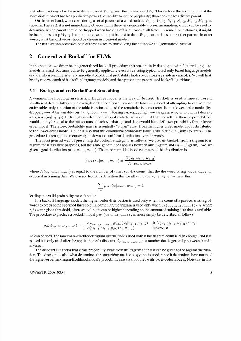
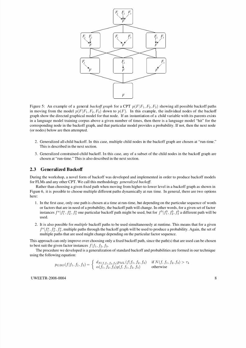
Figure 4: Left: An example of a general backoff graph for a CPT p(F |F 1, F 2, F 3) showing all possible backoff paths
in moving from the model p(F |F 1, F 2, F 3) down to p(F ). Right: An example of a backoff graph where only a subset
of the paths from the top to bottom are allowed. In this graph, the model p(F |F 1, F 2, F 3) is allowed only to backoff
to p(F |F 1, F 3) or p(F |F 2, F 3). This means that only the parents F 1 or F 2 may be dropped, but not parent F 3 sinceall backoff models must have parent F 3. Similarly, the model p(F |F 2, F 3) may backoff only to p(F |F 3), so only
the parent F 2 may be dropped in this case. This notion of specifying a subset of the parents that may be dropped to
determine a constrained set of backoff paths is used in the SRILM language-model toolkit [12] extensions, described
in Section 3.
Under the assumption that we always drop one parent at a time 3, we can see that there are quite a large number
of possible orders. We will refer to this as a backoff path, since it can be viewed as a path in a graph where each
node corresponds to a particular statistical model. When all paths are depicted, we get what we define as a backoff
graph as shown on the left in Figure 4 and Figure 5, the latter of which shows more explicitly the fact that each node
in the backoff graph corresponds to a particular statistical model. When training data for that statistical model is not
sufficient (below a threshold) in training data, then there is an option as to which next node in the backoff graph can
be used. In the example, the node p(F |F 1, F 2, F 3) has three options, those corresponding to dropping any one of the
three parents. The nodes p(F |F 1, F 2), p(F |F 1, F 3), and p(F |F 2, F 3) each have two options, and the nodes p(F |F 1), p(F |F 2), and p(F |F 3) each have only one option.
Given the above, we see that there are a number of possible options for choosing a backoff path, and these include:
1. Choose a fixed path from top to bottom based on what seems reasonable (as shown in Figure 6). An example
might be to always drop the most temporally distant parent when moving down levels in the backoff graph (as
is done with a typical word-based n-gram model). One might also choose the particular path based on other
linguistic knowledge about the given domain. Stems, for example, might be dropped before morphological
classes because it is believed that the morph classes possess more information about the word the stems. It is
also possible to choose the backoff path in a data-driven manner. The parent to be dropped first might be the
one which is found to possess the least information (in an information-theoretic sense) about the child variable.
Alternatively, it might be possible to choose the parent to drop first based on the tradeoff between statistical
predictability and statistical estimation. For example, we might choose to drop a parent which does not raise the
entropy the least if the child model is particularly easy to estimate given the current training data (i.e., the childmodel will have low statistical variance).
3It is possible to drop more than one parent during a backoff step (see Section 3.3 for an example). It is also possible to add parents at a backoff
step. This latter case is not further considered in this report.
UWEETR-2008-0004 7
8/12/2019 Tutorial on Factored Language Models
http://slidepdf.com/reader/full/tutorial-on-factored-language-models 9/39
F
1 F
2 F
3 F
F
F
3 F
F
2 F
F
1 F
F
2 F
3 F
F
1 F
3 F
F
1 F
2 F
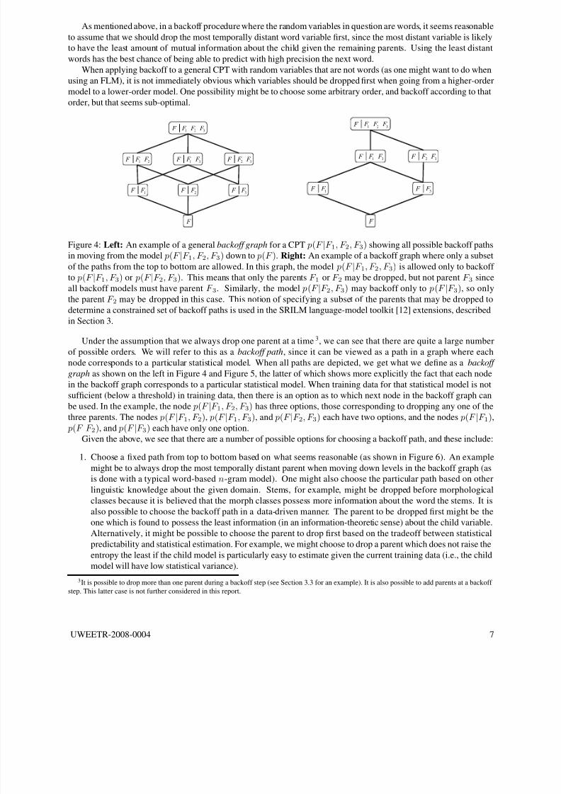
Figure 5: An example of a general backoff graph for a CPT p(F |F 1, F 2, F 3) showing all possible backoff paths
in moving from the model p(F |F 1, F 2, F 3) down to p(F ). In this example, the individual nodes of the backoff
graph show the directed graphical model for that node. If an instantiation of a child variable with its parents exists
in a language model training corpus above a given number of times, then there is a language model “hit” for thecorresponding node in the backoff graph, and that particular model provides a probability. If not, then the next node
(or nodes) below are then attempted.
2. Generalized all-child backoff. In this case, multiple child nodes in the backoff graph are chosen at “run-time.”
This is described in the next section.
3. Generalized constrained-child backoff. In this case, any of a subset of the child nodes in the backoff graph are
chosen at “run-time.” This is also described in the next section.
2.3 Generalized Backoff
During the workshop, a novel form of backoff was developed and implemented in order to produce backoff models
for FLMs and any other CPT. We call this methodology generalized backoff .Rather than choosing a given fixed path when moving from higher-to-lower level in a backoff graph as shown in
Figure 6, it is possible to choose multiple different paths dynamically at run time. In general, there are two options
here:
1. In the first case, only one path is chosen at a time at run-time, but depending on the particular sequence of words
or factors that are in need of a probability, the backoff path will change. In other words, for a given set of factor
instances f a|f a1 , f a2 , f a3 one particular backoff path might be used, but for f b|f b1 , f b2 , f b3 a different path will be
used.
2. It is also possible for multiple backoff paths to be used simultaneously at runtime. This means that for a given
f a|f a1 , f a2 , f a3 , multiple paths through the backoff graph will be used to produce a probability. Again, the set of
multiple paths that are used might change depending on the particular factor sequence.
This approach can only improve over choosing only a fixed backoff path, since the path(s) that are used can be chosen
to best suit the given factor instances f |f 1, f 2, f 3.
The procedure we developed is a generalization of standard backoff and probabilities are formed in our technique
using the following equation:
pGBO(f |f 1, f 2, f 3) =
dN (f,f 1,f 2,f 3) pML(f |f 1, f 2, f 3) if N (f, f 1, f 2, f 3) > τ 4α(f 1, f 2, f 3)g(f, f 1, f 2, f 3) otherwise
UWEETR-2008-0004 8
8/12/2019 Tutorial on Factored Language Models
http://slidepdf.com/reader/full/tutorial-on-factored-language-models 10/39
2 F
3 F
F 3
F
F 1
F 2
F 3
F
F
F F
F 1
F 2
F 3
F
F
1 F
2 F
F 2
F
F 1
F 2
F 3
F
F
F 1
F 3
F
F 1
F
F 1
F 2
F 3
F
F
F 1
F 2
F
F 1
F
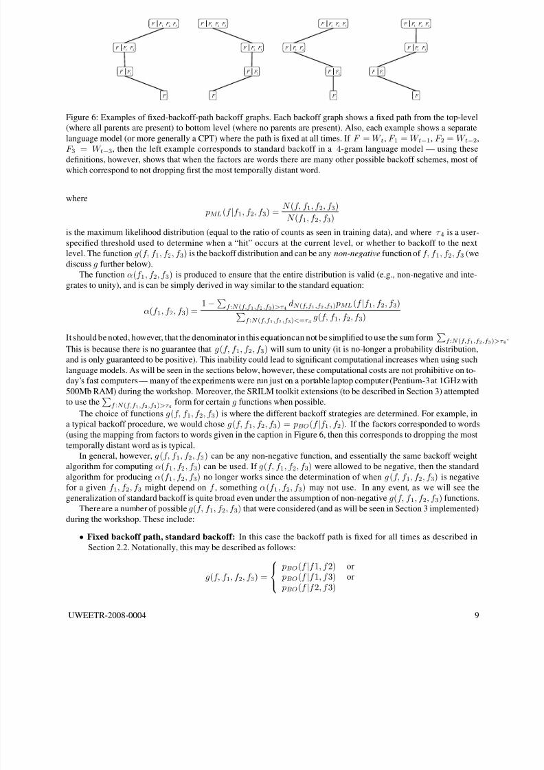
Figure 6: Examples of fixed-backoff-path backoff graphs. Each backoff graph shows a fixed path from the top-level
(where all parents are present) to bottom level (where no parents are present). Also, each example shows a separate
language model (or more generally a CPT) where the path is fixed at all times. If F = W t, F 1 = W t−1, F 2 = W t−2,
F 3 = W t−3, then the left example corresponds to standard backoff in a 4-gram language model — using these
definitions, however, shows that when the factors are words there are many other possible backoff schemes, most of
which correspond to not dropping first the most temporally distant word.
where
pML(f |f 1, f 2, f 3) = N (f, f 1, f 2, f 3)
N (f 1, f 2, f 3)
is the maximum likelihood distribution (equal to the ratio of counts as seen in training data), and where τ 4 is a user-
specified threshold used to determine when a “hit” occurs at the current level, or whether to backoff to the next
level. The function g(f, f 1, f 2, f 3) is the backoff distribution and can be any non-negative function of f, f 1, f 2, f 3 (we
discuss g further below).
The function α(f 1, f 2, f 3) is produced to ensure that the entire distribution is valid (e.g., non-negative and inte-
grates to unity), and is can be simply derived in way similar to the standard equation:
α(f 1, f 2, f 3) =1 −
f :N (f,f 1,f 2,f 3)>τ 4dN (f,f 1,f 2,f 3) pML(f |f 1, f 2, f 3)
f :N (f,f 1,f 2,f 3)<=τ 4g(f, f 1, f 2, f 3)
It should be noted, however, that the denominator in this equationcan not be simplified to use the sum form
f :N (f,f 1,f 2,f 3)>τ 4.
This is because there is no guarantee that g(f, f 1, f 2, f 3) will sum to unity (it is no-longer a probability distribution,
and is only guaranteed to be positive). This inability could lead to significant computational increases when using such
language models. As will be seen in the sections below, however, these computational costs are not prohibitive on to-
day’s fast computers — many of the experiments were run just on a portable laptop computer (Pentium-3 at 1GHz with
500Mb RAM) during the workshop. Moreover, the SRILM toolkit extensions (to be described in Section 3) attempted
to use the
f :N (f,f 1,f 2,f 3)>τ 4 form for certain g functions when possible.The choice of functions g(f, f 1, f 2, f 3) is where the different backoff strategies are determined. For example, in
a typical backoff procedure, we would chose g(f, f 1, f 2, f 3) = pBO(f |f 1, f 2). If the factors corresponded to words
(using the mapping from factors to words given in the caption in Figure 6, then this corresponds to dropping the most
temporally distant word as is typical.
In general, however, g(f, f 1, f 2, f 3) can be any non-negative function, and essentially the same backoff weight
algorithm for computing α(f 1, f 2, f 3) can be used. If g(f, f 1, f 2, f 3) were allowed to be negative, then the standard
algorithm for producing α(f 1, f 2, f 3) no longer works since the determination of when g (f, f 1, f 2, f 3) is negative
for a given f 1, f 2, f 3 might depend on f , something α(f 1, f 2, f 3) may not use. In any event, as we will see the
generalization of standard backoff is quite broad even under the assumption of non-negative g(f, f 1, f 2, f 3) functions.
There are a number of possible g(f, f 1, f 2, f 3) that were considered (and as will be seen in Section 3 implemented)
during the workshop. These include:
• Fixed backoff path, standard backoff: In this case the backoff path is fixed for all times as described inSection 2.2. Notationally, this may be described as follows:
g(f, f 1, f 2, f 3) =
pBO(f |f 1, f 2) or
pBO(f |f 1, f 3) or
pBO(f |f 2, f 3)
UWEETR-2008-0004 9
8/12/2019 Tutorial on Factored Language Models
http://slidepdf.com/reader/full/tutorial-on-factored-language-models 11/39
where the “or” means “exclusive or” (so one and only one choice is taken) and where the choice is decided by
the user and is fixed for all time. This case therefore includes standard backoff (as in a word n-gram) but also
allows for arbitrary fixed (but single) backoff-paths to be specified (see Figure 6).
• Max Counts: In this case, the backoff probability model is chosen based on the number of counts of the current
“gram” (i.e., random variable assignments). Specifically,
g(f, f 1, f 2, f 3) = pGBO(f |f 1 , f 2)
where
(1, 2) = argmax
(m1
,m2
)∈{(1,2),(1,3),(2,3)}
N (f, f m1, f m2
)
Because this is slightly notationally cumbersome, we here describe this approach in the case when there are only
two parents, thus giving the definition for g(f, f 1, f 2). In this case, the above equations can be written as:
g(f, f 1, f 2) = pGBO(f |f )
where
= argmaxj∈{1,2}
N (f, f j)
In other words, for each set of factor values, the backoff model chosen to be the one that corresponds to the
factor values that have maximum counts. This means that a different backoff path will be used for each instance,
and one will always backoff down the path of maximum counts. This approach tends to prefer backoff models
that have better (non-relative) statistical estimation properties, but it ignores the statistical predictability of theresulting backoff models.
• Max Normalized Counts: In this case, rather than the absolute counts, the normalized counts are used to
determine the backoff model. Thus,
g(f, f 1, f 2, f 3) = pGBO(f |f 1 , f 2)
where
(1, 2) = argmax(m1,m2)∈{(1,2),(1,3),(2,3)}
N (f, f m1, f m2
)
N (f m1, f m2
) = argmax
(m1,m2)∈{(1,2),(1,3),(2,3)}
pML(f |f m1, f m2
)
This approach therefore chooses the backoff model according to the one that has the highest probability score
using the maximum-likelihood distribution. This approach therefore favors models that yield high-predictability
possibly at the expense of statistical estimation quality.
• Max Num-Words Normalized Counts: In this case, the counts are normalized by the number of possible factor
values for a given set of parent values, as computed using the training set.
The set of possible factor values for a given parent context f 1, f 2, f 3 can be expressed as the following set:
{f : N (f, f 1, f 2, f 3) > 0}
and the number of possible following words is equal to the cardinality of this set. Using the standard notation to
express set cardinality, we obtain the following equations:
g(f, f 1, f 2, f 3) = pGBO(f |f 1 , f 2)
where(1, 2) = argmax
(m1,m2)∈{(1,2),(1,3),(2,3)}
N (f, f m1, f m2
)
|{f : N (f, f m1, f m2
) > 0}|
Note that if the factors correspond to words, then the normalization is equal to the number of possible following
words for a given history.
UWEETR-2008-0004 10

8/12/2019 Tutorial on Factored Language Models
http://slidepdf.com/reader/full/tutorial-on-factored-language-models 12/39
• Max Backoff-Graph Node Probability: In this approach, we choose the backoff model to be the one that gives
the factor and parent context in question the maximum probability. This can be written as:
g(f, f 1, f 2, f 3) = pGBO(f |f 1 , f 2)
where
(1, 2) = argmax(m1,m2)∈{(1,2),(1,3),(2,3)}
pGBO(f |f m1, f m2
)
This approach therefore chooses the next backoff graph node to be the one that supplies the highest probability,
but where the probability is itself obtained via using a backoff procedure.
• Max Product-of-Cardinality Normalized Counts: In this approach, the counts are normalized by the productof the cardinalities of the underlying random variables. In this case, we use the term “cardinality of a random
variable” to mean the number of possible values that random variable may take on in the training set. Again
using set notation, we will notate the cardinality of a random variable as |F |, where the cardinality of a random
variable F is taken to be:
|F | ∆= |{f : N (f ) > 0}|
This leads to:
g(f, f 1, f 2, f 3) = pGBO(f |f 1 , f 2)
where
(1, 2) = argmax(m1,m2)∈{(1,2),(1,3),(2,3)}
N (f, f m1, f m2
)
|F ||F m1||F m2
|
• Max Sum-of-Cardinality Normalized Counts: In this case the sum of the of the random variable cardinalities
are used for the normalization, giving:
g(f, f 1, f 2, f 3) = pGBO(f |f 1 , f 2)
where
(1, 2) = argmax(m1,m2)∈{(1,2),(1,3),(2,3)}
N (f, f m1, f m2
)
|F | + |F m1| + |F m2
|
• Max Sum-of-Log-Cardinality Normalized Counts: In this case the sum of the of the random variable natural
log cardinalities are used for the normalization, giving:
g(f, f 1, f 2, f 3) = pGBO(f |f 1 , f 2)
where
(1, 2) = argmax(m1,m2)∈{(1,2),(1,3),(2,3)}
N (f, f m1, f m2
)
ln |F | + ln |F m1| + ln |F m2
|
Several other g(f, f 1, f 2, f 3) functions were also implemented, including minimum versions of the above (these
are identical to the above except that the the argmin rather than the argmax function is used. Specifically,
• Min Counts
• Min Normalized Counts
• Min Num-Words Normalized Counts
• Min Backoff-Graph Node Probability• Min Product-of-Cardinality Normalized Counts
• Min Sum-of-Cardinality Normalized Counts
• Min Sum-of-Log-Cardinality Normalized Counts
UWEETR-2008-0004 11

8/12/2019 Tutorial on Factored Language Models
http://slidepdf.com/reader/full/tutorial-on-factored-language-models 13/39
Still, several more g(f, f 1, f 2, f 3) functions were implemented that take neither the min nor max of their argu-
ments. These include:
• Sum:
g(f, f 1, f 2, f 3) =
(m1,m2)∈{(1,2),(1,3),(2,3)}
pGBO(f |f m1, f m2
)
• Average (arithmetic mean):
g(f, f 1, f 2, f 3) = 1
3
(m1,m2)∈{(1,2),(1,3),(2,3)}
pGBO(f |f m1, f m2
)
• Product:
g(f, f 1, f 2, f 3) =
(m1,m2)∈{(1,2),(1,3),(2,3)}
pGBO(f |f m1, f m2
)
• Geometric Mean:
g(f, f 1, f 2, f 3) =
(m1,m2)∈{(1,2),(1,3),(2,3)}
pGBO(f |f m1, f m2
)
1/3
• Weighted Mean:
g(f, f 1, f 2, f 3) = (m1,m2)∈{(1,2),(1,3),(2,3)}
pγ m1,m2
GBO
(f |f m1, f m2
)
where the weights γ m1,m2 are specified by the user.
Note that these last examples correspond to approaches where multiple backoff paths are used to form a final
probability score rather than a single backoff path for a given factor value and context (as described earlier in this
section). Also note that rather taking the sum ( respectively average, product, etc.) over all children in the backoff
graph, it can be beneficial to take the sum (respectively average, product, etc.) over an a priori specified subset of the
children. As will be seen, this subset functionality (and all of the above) was implemented as extensions to the SRI
toolkit as described in the next section. Readers interested in the perplexity experiments rather than the details of the
implementation may wish to skip to Section 4.
3 FLM Programs in the SRI Language Model ToolkitSignificant code extensions were made to the SRI language modeling toolkit SRILM [12] by Jeff Bilmes and Andreas
Stolcke in order to support both factored language models and generalized backoff.
Essentially, the SRI toolkit was extended with a graphical-models-like syntax (similar to [2]) to specify a given
statistical model. A graph syntax was used to specify the given child variable and its parents, and then a specific syntax
was used to specify each possible node in the backoff graph (Figure 5), a set of node options (e.g., type of smoothing),
and the set of each nodes possible backoff-graph children. This therefore allowed the possibility to create backoff
graphs of the sort shown in the right of Figure 4. The following sections serve to provide complete documentation for
the extensions made to the SRILM toolkit.
3.1 New Programs: fngram and fngram-count
Two new programs have been added to the SRILM program suite. They are fngram and fngram-count. These
programs are analogous to the normal SRILM programs ngram and ngram-count but they behave in somewhat
different ways.
The program ngram-count will take a factored language data file (the format is described in Section 3.2) and
will produce both a count file and optionally a language model file. The options for this program are described below.
UWEETR-2008-0004 12

8/12/2019 Tutorial on Factored Language Models
http://slidepdf.com/reader/full/tutorial-on-factored-language-models 14/39
One thing to note about these options is that, unlike ngram-count, fngram-count does not include command-
line options for language model smoothing and discounting at each language model level. This is because potentially
a different set of options needs to be specified for each node in the backoff graph (Figure 3). Therefore, the smoothing
and discounting options are all specified in the language model description file, described in Section 3.3.
The following are the options for the fngram-count program, the program that takes a text (a stream of feature
bundles) and estimates factored count files and factored language models.
• -factor-file < str > Gives the name of the FLM description file that describes the FLM to use (See
Section 3.3).
• -debug < int > Gives debugging level for the program.
• -sort Sort the ngrams when written to the output file.
• -text < str > Text file to read in containing language model training information.
• -read-counts Try to read counts information from counts file first. Note that the counts file are specified in
the FLM file (Section 3.3).
• -write-counts Write counts to file(s). Note that the counts file are specified in the FLM file (Section 3.3).
• -write-counts-after-lm-train Write counts to file(s) after (rather than before) LM training. Note
that this can have an effect if Kneser-Ney or Modified Kneser-Ney smoothing is in effect, as the smoothing
method will change the internal counts. This means that without this option, the non Kneser-Ney counts will be
written.
• -lm
Estimate and write lm to file(s). If not given, just the counts will be computed.• -kn-counts-modified Input counts already modified for KN smoothing, so don’t do it internally again.
• -no-virtual-begin-sentence Do not use a virtual start sentence context at the sentence begin. A FLM
description file describes a model for a child variable C given its set of parent variables P 1, P 2, . . . , P N . The
parent variables can reside any distance into the past relative to the parent variable. Let us say that the maximum
number of feature bundles (i.e., time slots) into the past is equal to τ . When the child variable corresponds to
time slot greater than τ it is always possible to obtain a true parent variable value for LM training. Near the
beginning of sentences (i.e., at time slots less than τ ) there are no values for one or more parent variable. The
normal behavior in this case is to assume a virtual start of sentence value for all of these parent values (so we can
think of a sentence as containing an infinite number of start of sentence tokens extending into the past relative
to the beginning of the sentence). For example, if an FLM specified a simple trigram model over words, the
following contexts would be used at the beginning of a sentence: < s > < s > w1, < s > w1 w2, w1 w2
w3, and so on.
This is not the typical behavior of SRILM in the case of a trigram, and in order to recover the typical behav-
ior, this option can be used, meaning do not add virtual start of sentence tokens before the beginning of each
sentence.
Note that for an FLM simulating a word-based n gram, if you want to get exactly the same smoothed language
model probabilities as the standard SRILM programs, you need to include the options -no-virtual-begin-senten
and -nonull, and make sure gtmin options in the FLM are the same as specified on the command line for
the usual SRILM programs.
• -keepunk Keep the symbol < unk > in LM. When < unk > is in the language model, each factor automat-
ically will contain a special < unk > symbol that becomes part of the valid set of values for a tag. If < unk >is in the vocabulary, then probabilities will (typically) be given for an instance of this symbol even if it does
not occur in the training data (because of backoff procedure smoothing, assuming the FLM options use such
backoff).
If < unk > is not in the language model (and it did not occur in training data), then zero probabilities will be
returned in this case. If this happens, and the child is equal to the < unk > value, then that will be considered
an out-of-vocabulary instance, and a special counter will be incremented (and corresponding statistics reported).
This is similar to the standard behavior of SRILM.
UWEETR-2008-0004 13

8/12/2019 Tutorial on Factored Language Models
http://slidepdf.com/reader/full/tutorial-on-factored-language-models 15/39
• -nonull Remove < NULL > from LM. Normally the special word < NULL > is included as a special
value for all factors in a FLM. This means that the language model smoothing will also smooth over (and
therefore give probability to) the < NULL > token. This option says to remove < NULL > as a special
token in the FLM (unless it is encountered in the training data for a particular factor).
Note that for an FLM simulating a word-based n gram, if you want to get exactly the same smoothed language
model probabilities as the standard SRILM programs, you need to include the options -no-virtual-begin-senten
and -nonull, and make sure gtmin options in the FLM are the same as specified on the command line for
the usual SRILM programs.
• -meta-tag Meta tag used to input count-of-count information. Similar to the other SRILM programs.
• -tolower Map vocabulary to lowercase. Similar to the other SRILM programs.
• -vocab vocab file. Read in the vocabulary specified by the vocab file. This also means that the vocabulary is
closed, and anything not in the vocabulary is seen as an OOV.
• -non-event non-event word. The ability to specify another “word” that is set to be a special non-event
word. A non-event word is one that is not smoothed over (so if it is in the vocabulary, it still won’t effect LM
probabilities). Note that since we are working with FLMs, you need to specify the corresponding tag along with
the word in order to get the correct behavior. For example, you would need to specify the non-event word as
“P-noun” for a part of speech factor, where “P” is the tag. Non-events don’t count as part of the vocabulary
(e.g., the size of the vocabulary), contexts (i.e., parent random variable values) which contain non-events are not
estimated or included in a resulting language model, and so on.
• -nonevents non-event vocabulary file. Specifies a file that contains a list of non-event words — good if you
need to specify more than one additional word as a non-event word.
• -write-vocab write vocab to file. Says that the current vocabulary should be written to a file.
The following are the options for the fngram program. This program uses the counts and factored language models
previously computed, and can either compute perplexity on another file, or can re-score n-best lists. The n-best list
rescoring is similar to the
• -factor-file build a factored LM, use factors given in file. Same as in fngram-count.
• -debug debugging level for lm. Same as in fngram-count.
• -skipoovs skip n-gram contexts containing OOVs.
• -unk vocabulary contains < unk > Same as in fngram-count.
• -nonull remove < NU LL > in LM. Same as in fngram-count.
• -tolower map vocabulary to lowercase. Same as in fngram-count.
• -ppl text file to compute perplexity from. This specifies a text file (a sequence of feature bundles) on which
perplexity should be computed. Note that multiple FLMs from the FLM file might be used to compute perplexity
from this file simultaneously. See Section 3.3.
• -escape escape prefix to pass data through. Lines that begin with this are printed to the output.
• -seed seed for randomization.
• -vocab vocab file. Same as in fngram-count.
• -non-event non-event word. Same as in fngram-count.
• -nonevents non-event vocabulary file. Same as in fngram-count.
• -write-lm re-write LM to file. Write the LM to the LM files specified in the FLM specification file.
UWEETR-2008-0004 14
8/12/2019 Tutorial on Factored Language Models
http://slidepdf.com/reader/full/tutorial-on-factored-language-models 16/39
• -write-vocab write LM vocab to file. Same as in fngram-count.
• -rescore hyp stream input file to rescore. This is similar to the -rescore option in the program ngram
(i.e., ngram supports a number of different ways of doing n-best rescoring, while fngram supports only one,
namely the one corresponding to the -rescore option).
• -separate-lm-scores print separate lm scores in n-best file. Since an FLM file might contain multiple
FLMs, this option says that separate scores for each FLM and for each item in the n-best file should be printed,
rather than combining them into one score. This would be useful to, at a later stage, combine the scores for
doing language-model weighting.
• -rescore-lmw rescoring LM weight. The weight to apply to the language model scores when doing rescor-ing.
• -rescore-wtw rescoring word transition weight. The weight to apply to a word transition when doing rescor-
ing.
• -noise noise tag to skip, similar to the normal SRILM programs.
• -noise-vocab noise vocabulary to skip, but a list contained in a file. Similar to the normal SRILM programs.
3.2 Factored Language Model Training Data File Format
Typically, language data consists of a set of words which are used to train a given language model. For an FLM, each
word might be accompanied by a number of factors. Therefore, rather than a stream of words, a stream of vectors must
be specified, since a factored language model can be seen to be a model over multiple streams of data, each streamcorresponding to a given factor as it evolves over time.
To support such a representation, language model files are assumed to be a stream of feature bundles, where each
feature in the bundle is separated from the next by the “:” (colon) character, and where each feature consists of a
< tag >-< value > pair.4 The < tag > can be any string (of any length), and the toolkit will automatically
identify the tag strings in a training data file with the corresponding string in the language-model specification file (to
be described below). The < value > can be any string that will, by having it exist in the training file, correspond to a
valid value of that particular tag. The tag and value are separated by a dash “-” character.
A language model training file may contain many more tag-value pairs than are used in a language model specifi-
cation file — the extra tag-value pairs are simply ignored. Each feature bundle, however, may only have one instance
of a particular tag. Also, if for a given feature a tag is missing, then it is assumed to be the special tag “W” which
typically will indicate that the value is a word. Again, this can happen only one time in a given bundle.
A given tag-value pair may also be missing from a feature bundle. In such a case, it is assumed that the tag exists,
but has the special value “NULL” which indicates a missing tag (note that the behavior for the start and end of sentenceword is different, see below). This value may also be specified explicitly in a feature bundle, such as S-NULL. If there
are many such NULLs in a given training file, it could reduce file size by not explicitly stating them and using this
implicit mechanism.
The following are a number of examples of training files:
the brown dog ate a bone
In this first example, the language model file consists of a string of what are (presumably) words that have not been
tagged. It is therefore assumed that they are words. The sentence is equivalent to the following where the word tags
are explicitly given:
W-the W-brown W-dog W-ate W-a W-bone
If we then wanted to also include part-of-speech information as a separate tag and using the string “ P” to identify
part of speech, then could would be specified as follows:
4Note, that the tag can be any tag such as a purely data-driven word class, and need not necessarily be a lexical tag or other linguistic part-of-
speech tag. The name “tag” here therefore is used to represent any feature.
UWEETR-2008-0004 15
8/12/2019 Tutorial on Factored Language Models
http://slidepdf.com/reader/full/tutorial-on-factored-language-models 17/39
W-the:P-article W-brown:P-adjective W-dog:P-noun
W-ate:P-verb W-a:P-article W-bone:P-noun
The order of the individual features within a bundle do not matter, so the above example is identical to the follow-
ing:
P-article:W-the P-adjective:W-brown P-noun:W-dog
P-verb:W-ate P-article:W-a P-noun:W-bone
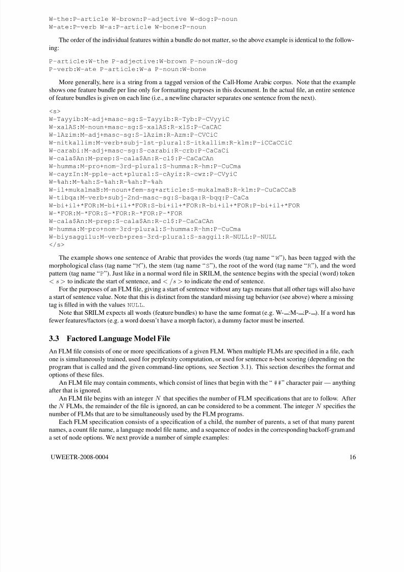
More generally, here is a string from a tagged version of the Call-Home Arabic corpus. Note that the example
shows one feature bundle per line only for formatting purposes in this document. In the actual file, an entire sentence
of feature bundles is given on each line (i.e., a newline character separates one sentence from the next).
<s>
W-Tayyib:M-adj+masc-sg:S-Tayyib:R-Tyb:P-CVyyiC
W-xalAS:M-noun+masc-sg:S-xalAS:R-xlS:P-CaCAC
W-lAzim:M-adj+masc-sg:S-lAzim:R-Azm:P-CVCiC
W-nitkallim:M-verb+subj-1st-plural:S-itkallim:R-klm:P-iCCaCCiC
W-carabi:M-adj+masc-sg:S-carabi:R-crb:P-CaCaCi
W-cala$An:M-prep:S-cala$An:R-cl$:P-CaCaCAn
W-humma:M-pro+nom-3rd-plural:S-humma:R-hm:P-CuCma
W-cayzIn:M-pple-act+plural:S-cAyiz:R-cwz:P-CVyiC
W-%ah:M-%ah:S-%ah:R-%ah:P-%ah
W-il+mukalmaB:M-noun+fem-sg+article:S-mukalmaB:R-klm:P-CuCaCCaB
W-tibqa:M-verb+subj-2nd-masc-sg:S-baqa:R-bqq:P-CaCaW-bi+il+*FOR:M-bi+il+*FOR:S-bi+il+*FOR:R-bi+il+*FOR:P-bi+il+*FOR
W-*FOR:M-*FOR:S-*FOR:R-*FOR:P-*FOR
W-cala$An:M-prep:S-cala$An:R-cl$:P-CaCaCAn
W-humma:M-pro+nom-3rd-plural:S-humma:R-hm:P-CuCma
W-biysaggilu:M-verb+pres-3rd-plural:S-saggil:R-NULL:P-NULL
</s>
The example shows one sentence of Arabic that provides the words (tag name “ W”), has been tagged with the
morphological class (tag name “M”), the stem (tag name “S”), the root of the word (tag name “R”), and the word
pattern (tag name “P”). Just like in a normal word file in SRILM, the sentence begins with the special (word) token
< s > to indicate the start of sentence, and < /s > to indicate the end of sentence.
For the purposes of an FLM file, giving a start of sentence without any tags means that all other tags will also have
a start of sentence value. Note that this is distinct from the standard missing tag behavior (see above) where a missing
tag is filled in with the values NULL.
Note that SRILM expects all words (feature bundles) to have the same format (e.g. W- :M- :P- ). If a word has
fewer features/factors (e.g. a word doesn’t have a morph factor), a dummy factor must be inserted.
3.3 Factored Language Model File
An FLM file consists of one or more specifications of a given FLM. When multiple FLMs are specified in a file, each
one is simultaneously trained, used for perplexity computation, or used for sentence n-best scoring (depending on the
program that is called and the given command-line options, see Section 3.1). This section describes the format and
options of these files.
An FLM file may contain comments, which consist of lines that begin with the “ ##” character pair — anything
after that is ignored.
An FLM file begins with an integer N that specifies the number of FLM specifications that are to follow. Afterthe N FLMs, the remainder of the file is ignored, an can be considered to be a comment. The integer N specifies the
number of FLMs that are to be simultaneously used by the FLM programs.
Each FLM specification consists of a specification of a child, the number of parents, a set of that many parent
names, a count file name, a language model file name, and a sequence of nodes in the corresponding backoff-gram and
a set of node options. We next provide a number of simple examples:
UWEETR-2008-0004 16
8/12/2019 Tutorial on Factored Language Models
http://slidepdf.com/reader/full/tutorial-on-factored-language-models 18/39
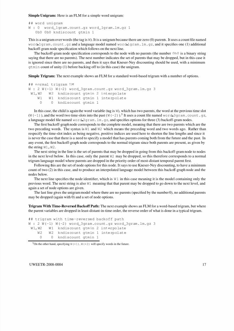
Simple Unigram: Here is an FLM for a simple word unigram:
## word unigram
W : 0 word_1gram.count.gz word_1gram.lm.gz 1
0b0 0b0 kndiscount gtmin 1
This is a unigram over words (the tag is W). It is a unigram because there are zero (0) parents. It uses a count file named
word 1gram.count.gz and a language model named word 1gram.lm.gz, and it specifies one (1) additional
backoff-gram node specification which follows on the next line.
The backoff-gram node specification corresponds to the node with no parents (the number 0b0 is a binary string
saying that there are no parents). The next number indicates the set of parents that may be dropped, but in this case itis ignored since there are no parents, and then it says that Kneser-Ney discounting should be used, with a minimum
gtmin count of unity (1) before backing off to (in this case) the unigram.
Simple Trigram: The next example shows an FLM for a standard word-based trigram with a number of options.
## normal trigram LM
W : 2 W(-1) W(-2) word_3gram.count.gz word_3gram.lm.gz 3
W1,W2 W2 kndiscount gtmin 2 interpolate
W1 W1 kndiscount gtmin 1 interpolate
0 0 kndiscount gtmin 1
In this case, the child is again the word variable (tag is W), which has two parents, the word at the previous time slot
(W(-1)), and the word two time-slots into the past (W(-2)).5
It uses a count file named word 3gram.count.gz,a language model file named word 3gram.lm.gz, and specifies options for three (3) backoff-gram nodes.
The first backoff-graph node corresponds to the complete model, meaning that there are two parents which are the
two preceding words. The syntax is W1 and W2 which means the preceding word and two words ago. Rather than
respecify the time-slot index as being negative, positive indices are used here to shorten the line lengths and since it
is never the case that there is a need to specify a model that has parents coming both from the future and the past. In
any event, the first backoff-graph node corresponds to the normal trigram since both parents are present, as given by
the string W1,W2.
The next string in the line is the set of parents that may be dropped in going from this backoff-gram node to nodes
in the next level below. In this case, only the parent W2 may be dropped, so this therefore corresponds to a normal
trigram language model where parents are dropped in the priority order of most-distant temporal parent first.
Following this are the set of node options for this node. It says to use Kneser-Ney discounting, to have a minimum
count of two (2) in this case, and to produce an interpolated language model between this backoff-graph node and the
nodes below.The next line specifies the node identifier, which is W1 in this case meaning it is the model containing only the
previous word. The next string is also W1 meaning that that parent may be dropped to go down to the next level, and
again a set of node options are given.
The last line gives the unigram model where there are no parents (specified by the number 0), no additional parents
may be dropped (again with 0) and a set of node options.
Trigram With Time-Reversed Backoff Path: The next example shows an FLM for a word-based trigram, but where
the parent variables are dropped in least-distant-in-time order, the reverse order of what is done in a typical trigram.
## trigram with time-reversed backoff path
W : 2 W(-1) W(-2) word_3gram.count.gz word_3gram.lm.gz 3
W1,W2 W1 kndiscount gtmin 2 interpolate
W2 W2 kndiscount gtmin 1 interpolate0 0 kndiscount gtmin 1
5On the other hand, specifying W(+1), W(+2) will specify words in the future.
UWEETR-2008-0004 17
8/12/2019 Tutorial on Factored Language Models
http://slidepdf.com/reader/full/tutorial-on-factored-language-models 19/39
As can be seen, the backoff graph node for the case where two parents are present (node W1,W2) says that only one
parent can be dropped, but in this case that parent is W1. This means that the next node to be used in the backoff graph
corresponds to the model p(W t|W t−2). It should be understood exactly what counts are used to produce this model.
p(W t|W t−2) corresponds to the use of counts over a distance of two words, essentially integrating all possible words in
between those two words. In other words, this model will use the counts N (wt−2, wt) =
wt−1N (wt−2, wt−1, wt) to
produce, in the maximum likelihood case (i.e., no smoothing), the model pML(W t|W t−2) = N (wt−2, wt)/N (wt−2)where N (wt−2) =
wt
N (wt−2, wt).
Note that this model is quite distinct from the case where the model p(W t|W t−1) is used, but where the word
from two time slots ago is substituted into the position of the previous word (this is what a SRILM skip-n-gram
would do). We use the following notation to make the distinction. The FLM above corresponds to the case where
P (W t = wt|W t−2 = wt−2) is used for the backoff-graph node probability. A skip-n-gram, on the other hand, wouldutilize (for the sake of interpolation) P (W t = wt|W t−1 = wt−2) where the random variable W t−1 is taken to have
the value of the word wt−2 from two time-slots into the past. In this latter case, the same actual counts are used
N (wt, wt−1) to produce the probability, only the word value is changed. In the former case, an entirely different count
quantity N (wt, wt−2) is used.
Note that a skip-n-gram would not work in the case where the parents correspond to different types of random
variables (e.g., if parents were words, stems, morphs, and so on). For example, if one parent is a word and another is
a stem, one could not substitute the stem in place of the word unless a super-class is created that is the union of both
words and stems. Such a super-class could have an effect on smoothing (in particular for the Kneser-Ney case) and
table storage size. A FLM allows different random variable types to be treated differently in each parent variable, and
allows counts to be computed separately for each subset of parents.
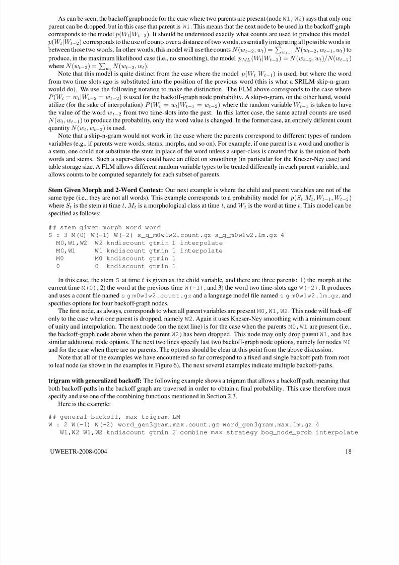
Stem Given Morph and 2-Word Context: Our next example is where the child and parent variables are not of the
same type (i.e., they are not all words). This example corresponds to a probability model for p(S t|M t, W t−1, W t−2)where S t is the stem at time t, M t is a morphological class at time t, and W t is the word at time t. This model can be
specified as follows:
## stem given morph word word
S : 3 M(0) W(-1) W(-2) s_g_m0w1w2.count.gz s_g_m0w1w2.lm.gz 4
M0,W1,W2 W2 kndiscount gtmin 1 interpolate
M0,W1 W1 kndiscount gtmin 1 interpolate
M0 M0 kndiscount gtmin 1
0 0 kndiscount gtmin 1
In this case, the stem S at time t is given as the child variable, and there are three parents: 1) the morph at the
current time M(0), 2) the word at the previous time W(-1), and 3) the word two time-slots ago W(-2). It produces
and uses a count file named s g m0w1w2.count.gz and a language model file named s g m0w1w2.lm.gz, andspecifies options for four backoff-graph nodes.
The first node, as always, corresponds to when all parent variables are present M0,W1,W2. This node will back-off
only to the case when one parent is dropped, namely W2. Again it uses Kneser-Ney smoothing with a minimum count
of unity and interpolation. The next node (on the next line) is for the case when the parents M0,W1 are present (i.e.,
the backoff-graph node above when the parent W2) has been dropped. This node may only drop parent W1, and has
similar additional node options. The next two lines specify last two backoff-graph node options, namely for nodes M0
and for the case when there are no parents. The options should be clear at this point from the above discussion.
Note that all of the examples we have encountered so far correspond to a fixed and single backoff path from root
to leaf node (as shown in the examples in Figure 6). The next several examples indicate multiple backoff-paths.
trigram with generalized backoff: The following example shows a trigram that allows a backoff path, meaning that
both backoff-paths in the backoff graph are traversed in order to obtain a final probability. This case therefore must
specify and use one of the combining functions mentioned in Section 2.3.Here is the example:
## general backoff, max trigram LM
W : 2 W(-1) W(-2) word_gen3gram.max.count.gz word_gen3gram.max.lm.gz 4
W1,W2 W1,W2 kndiscount gtmin 2 combine max strategy bog_node_prob interpolate
UWEETR-2008-0004 18
8/12/2019 Tutorial on Factored Language Models
http://slidepdf.com/reader/full/tutorial-on-factored-language-models 20/39
W2 W2 kndiscount gtmin 1 interpolate
W1 W1 kndiscount gtmin 1 interpolate
0 0 kndiscount gtmin 1 kn-count-parent 0b11
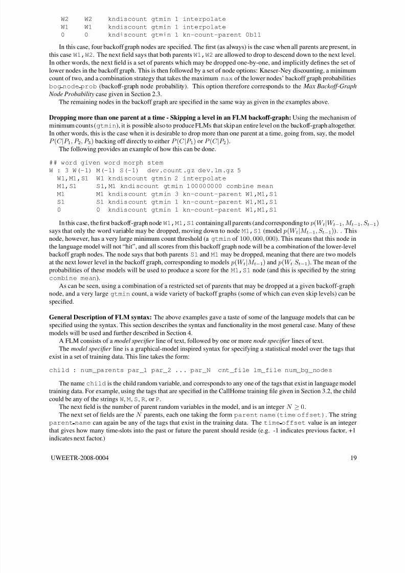
In this case, four backoff graph nodes are specified. The first (as always) is the case when all parents are present, in
this case W1,W2. The next field says that both parents W1,W2 are allowed to drop to descend down to the next level.
In other words, the next field is a set of parents which may be dropped one-by-one, and implicitly defines the set of
lower nodes in the backoff graph. This is then followed by a set of node options: Kneser-Ney discounting, a minimum
count of two, and a combination strategy that takes the maximum max of the lower nodes’ backoff graph probabilities
bog node prob (backoff-graph node probability). This option therefore corresponds to the Max Backoff-Graph
Node Probability case given in Section 2.3.
The remaining nodes in the backoff graph are specified in the same way as given in the examples above.
Dropping more than one parent at a time - Skipping a level in an FLM backoff-graph: Using the mechanism of
minimum counts (gtmin), it is possible also to produce FLMs that skip an entire level on the backoff-graph altogether.
In other words, this is the case when it is desirable to drop more than one parent at a time, going from, say, the model
P (C |P 1, P 2, P 3) backing off directly to either P (C |P 1) or P (C |P 2).
The following provides an example of how this can be done.
## word given word morph stem
W : 3 W(-1) M(-1) S(-1) dev.count.gz dev.lm.gz 5
W1,M1,S1 W1 kndiscount gtmin 2 interpolate
M1,S1 S1,M1 kndiscount gtmin 100000000 combine mean
M1 M1 kndiscount gtmin 3 kn-count-parent W1,M1,S1
S1 S1 kndiscount gtmin 1 kn-count-parent W1,M1,S10 0 kndiscount gtmin 1 kn-count-parent W1,M1,S1
In this case, the first backoff-graph node W1,M1,S1 containing all parents (and corresponding to p(W t|W t−1, M t−1, S t−1)says that only the word variable may be dropped, moving down to node M1,S1 (model p(W t|M t−1, S t−1)). . This
node, however, has a very large minimum count threshold (a gtmin of 100, 000, 000). This means that this node in
the language model will not “hit”, and all scores from this backoff graph node will be a combination of the lower-level
backoff graph nodes. The node says that both parents S1 and M1 may be dropped, meaning that there are two models
at the next lower level in the backoff graph, corresponding to models p(W t|M t−1) and p(W t|S t−1). The mean of the
probabilities of these models will be used to produce a score for the M1,S1 node (and this is specified by the string
combine mean).
As can be seen, using a combination of a restricted set of parents that may be dropped at a given backoff-graph
node, and a very large gtmin count, a wide variety of backoff graphs (some of which can even skip levels) can be
specified.
General Description of FLM syntax: The above examples gave a taste of some of the language models that can be
specified using the syntax. This section describes the syntax and functionality in the most general case. Many of these
models will be used and further described in Section 4.
A FLM consists of a model specifier line of text, followed by one or more node specifier lines of text.
The model specifier line is a graphical-model inspired syntax for specifying a statistical model over the tags that
exist in a set of training data. This line takes the form:
child : num_parents par_1 par_2 ... par_N cnt_file lm_file num_bg_nodes
The name child is the child random variable, and corresponds to any one of the tags that exist in language model
training data. For example, using the tags that are specified in the CallHome training file given in Section 3.2, the child
could be any of the strings W, M, S, R, or P.The next field is the number of parent random variables in the model, and is an integer N ≥ 0.
The next set of fields are the N parents, each one taking the form parent name(time offset). The string
parent name can again be any of the tags that exist in the training data. The time offset value is an integer
that gives how many time-slots into the past or future the parent should reside (e.g. -1 indicates previous factor, +1
indicates next factor.)
UWEETR-2008-0004 19

8/12/2019 Tutorial on Factored Language Models
http://slidepdf.com/reader/full/tutorial-on-factored-language-models 21/39
What follows is a name to be used for the count file (keeping language model counts) and then the name of the
language model file. Note that both count files and language model file are specified since counts are, for certain cases
as described in Section 2.3, needed to determine the backoff probability.
The last field on the line is num bg nodes, which is the number of backoff-graph node specifications that are
following. Only the next such-number of lines are assumed to be part of the FLM file (anything after that is either
ignored, or is assumed to be part of the next FLM specified in the file). One should be careful to ensure that the number
of actual backoff-graph node specifiers given is equal to this number, as it is easy to add more node specifiers while
forgetting to update this field.
Once the model specifier is given, it is followed by num bg nodes model specifier s. Each model specifier consists
of the following form:
parent_list drop_list [node options]
The parent list is a comma-separated list (without spaces) of parent variables that correspond to this node. In
other words, each node in a backoff graph can be identified with a set of parent variables, and this string identifies the
node by giving that set. The parents are specified in a shortened syntax — each parent is given using its name (again
one of the tags in the file), and the absolute value of the time offset with no space. Examples of parent lists include
W1,W2,W3 to give the three preceding words, W1,M1,S1 to give the preceding word, morph, and stem, and so on.
The next field drop list gives the list of parents that may be dropped one at a time from this backoff-graph
node. This is the field that specifies the set of lower-level backoff-graph nodes that are used in case there is not a
language-model “hit” at this level. For example, if parent list is W1,M1,S1 and drop list is W1, then the
only next lower-level node used is the one with parent list M1,S1. If, on the other hand, a drop list of
W1,M1,S1 is used for parent list W1,M1,S1, then three nodes are used for the next lower-level — namely, the nodes
with parent lists M1,S1, W1,S1, and W1,M1.
The node options are one or more option for this backoff-graph node. Each backoff-graph node can have its own
discounting, smoothing, combination options, and so on. Many of the node options are similar to the command-line
options that can be given to the SRLIM program ngram-count. These options are included in the FLM file because
a different set might be given for each node. The following gives a list of all the node options that are currently
supported.
• gtmin [num] the lower GT discounting cutoff. When not using Good-Turing discounting, this gives the
threshold that the count needs to meet or exceed in order for there to be a language model “hit” at this backoff
graph node. Therefore, gtmin corresponds to the τ variables in the equations given in Section 2.
• gtmax [num] upper GT discounting cutoff. Note that if only this and gtmin are specified, then Good-Turing
smoothing is used.
• gt [fileName string] Good-Turing discount parameter file for this node.
• cdiscount [double] Says that constant discounting should be used, and this gives the discounting con-
stant.
• ndiscount Says that natural discounting should be used.
• wbdiscount Says that Witten-Bell discounting should be used.
• kndiscount Says that modified Kneser-Ney discounting should be used.
• ukndiscount Says that unmodified (i.e., the original or normal) Kneser-Ney discounting should be used.
• kn-counts-modified says that the input counts already modified for KN smoothing (this is similar to
ngram-count.
• kn-counts-modify-at-end says that the counts should be turned into KN-counts after discount estima-
tion rather than before. In other words, if this option is specified, the quantities such as n1, n2, n3, n4, and so
on (typically used for modified KN discounting) should be computed from the usual counts rather than from the
meta-meta-counts needed for Kneser-Ney smoothing.
UWEETR-2008-0004 20

8/12/2019 Tutorial on Factored Language Models
http://slidepdf.com/reader/full/tutorial-on-factored-language-models 22/39
• kn [fileName string] The Kneser-Ney discount parameter file for this backoff-graph node.
• kn-count-parent [parent spec] The backoff-graph parent that is used to compute the meta-meta-
counts needed for Kneser-Ney smoothing. Normally, the parent is the node immediately above the current node
in the backoff graph, but it is sometimes useful to specify a different parent, especially when the set of parents do
not correspond to the same random variables at different times (i.e., when the parents are truly different random
variables).
• interpolate use interpolated estimates for computing the probabilities for this node. In other words, the
probabilities should be interpolated with hits in the current nodes and whatever the g() function returns for the
lower node probabilities. This is therefore a generalization of the interpolated option in ngram-count.
• write [fileName string] Write the counts, just of this node alone, to the given file.
• combine [option] This option is active only when there multiple backoff paths (backoff-graph children)
possible (i.e., when the drop list specifies more than one parent variable. See Section 2.3. In this case,
[option] is one of:
– max the maximum of the next backoff-graph level nodes. This is the default if no combine option is
given.
– min the maximum of the next backoff-graph level nodes
– sum the maximum of the next backoff-graph level nodes
– avg||mean the arithmetic average (mean) of the next backoff-graph level nodes
– prod the product of the next backoff-graph level nodes
– gmean the geometric mean of the next backoff-graph level nodes
– wmean [ < node specweight > < node specweight > ... ] the weighted mean of the next
backoff-graph level nodes. The weights are given by providing a node specification (a list of comma
separated parents) to identify the node, and then a weight for that node. For example, one might used:
wmean W1,M2 7 W1,S2 3
which means that backoff-grpah node W1,M2 has a weight of 7, and node W1,S2 has a weight of 3.
• strategy [option] This option also is active only when there are multiple backoff paths (backoff-graph
children) possible, and when the combine option above is either min or max. See Section 2.3 for more
information. In this case, [option] is one of:
– counts sum counts norm The Max/Min Normalized Counts cases in Section 2.3. This is the default
case if no strategy option is given.
– counts no norm The Max/Min Counts cases in Section 2.3.
– counts sum num words norm The Max/Min Num-Words Normalized Counts cases in Section 2.3.
– counts prod card norm The Max/Min Product-of-Cardinality Normalized Counts cases in Sec-
tion 2.3.
– counts sum card norm The Max/Min Sum-of-Cardinality Normalized Counts cases in Section 2.3.
– counts sum log card norm The Max/Min Sum-of-Log-Cardinality Normalized Counts cases in Sec-
tion 2.3.
– bog node prob The Max/Min Backoff-Graph Node Probability cases in Section 2.3.
Other ways to specify backoff-graph nodes and drop sets. A backoff graph node is typically identified using acomma separated list of parents. Similarly, a set of parents that may be dropped is also specified using such a list. In
some cases, specifying these lists can be tedious, and it might be more concise (albeit more error prone) to specify
nodes and sets using a numeric representation.
Each parent list may also be specified using an integer, where the integer is a bit representation of the parents in
the set. When the line in the FLM file is given of the form:
UWEETR-2008-0004 21
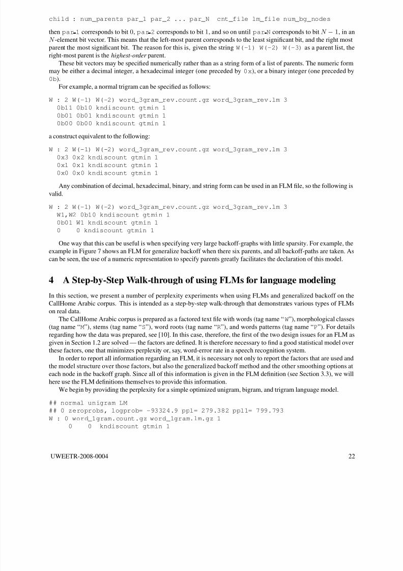
8/12/2019 Tutorial on Factored Language Models
http://slidepdf.com/reader/full/tutorial-on-factored-language-models 23/39
child : num_parents par_1 par_2 ... par_N cnt_file lm_file num_bg_nodes
then par 1 corresponds to bit 0, par 2 corresponds to bit 1, and so on until par N corresponds to bit N − 1, in an
N -element bit vector. This means that the left-most parent corresponds to the least significant bit, and the right most
parent the most significant bit. The reason for this is, given the string W(-1) W(-2) W(-3) as a parent list, the
right-most parent is the highest-order parent.
These bit vectors may be specified numerically rather than as a string form of a list of parents. The numeric form
may be either a decimal integer, a hexadecimal integer (one preceded by 0x), or a binary integer (one preceded by
0b).
For example, a normal trigram can be specified as follows:
W : 2 W(-1) W(-2) word_3gram_rev.count.gz word_3gram_rev.lm 30b11 0b10 kndiscount gtmin 1
0b01 0b01 kndiscount gtmin 1
0b00 0b00 kndiscount gtmin 1
a construct equivalent to the following:
W : 2 W(-1) W(-2) word_3gram_rev.count.gz word_3gram_rev.lm 3
0x3 0x2 kndiscount gtmin 1
0x1 0x1 kndiscount gtmin 1
0x0 0x0 kndiscount gtmin 1
Any combination of decimal, hexadecimal, binary, and string form can be used in an FLM file, so the following is
valid.
W : 2 W(-1) W(-2) word_3gram_rev.count.gz word_3gram_rev.lm 3
W1,W2 0b10 kndiscount gtmin 1
0b01 W1 kndiscount gtmin 1
0 0 kndiscount gtmin 1
One way that this can be useful is when specifying very large backoff-graphs with little sparsity. For example, the
example in Figure 7 shows an FLM for generalize backoff when there six parents, and all backoff-paths are taken. As
can be seen, the use of a numeric representation to specify parents greatly facilitates the declaration of this model.
4 A Step-by-Step Walk-through of using FLMs for language modeling
In this section, we present a number of perplexity experiments when using FLMs and generalized backoff on the
CallHome Arabic corpus. This is intended as a step-by-step walk-through that demonstrates various types of FLMs
on real data.
The CallHome Arabic corpus is prepared as a factored text file with words (tag name “ W”), morphological classes
(tag name “M”), stems (tag name “S”), word roots (tag name “R”), and words patterns (tag name “P”). For details
regarding how the data was prepared, see [10]. In this case, therefore, the first of the two design issues for an FLM as
given in Section 1.2 are solved — the factors are defined. It is therefore necessary to find a good statistical model over
these factors, one that minimizes perplexity or, say, word-error rate in a speech recognition system.
In order to report all information regarding an FLM, it is necessary not only to report the factors that are used and
the model structure over those factors, but also the generalized backoff method and the other smoothing options at
each node in the backoff graph. Since all of this information is given in the FLM definition (see Section 3.3), we will
here use the FLM definitions themselves to provide this information.
We begin by providing the perplexity for a simple optimized unigram, bigram, and trigram language model.
## normal unigram LM
## 0 zeroprobs, logprob= -93324.9 ppl= 279.382 ppl1= 799.793
W : 0 word_1gram.count.gz word_1gram.lm.gz 1
0 0 kndiscount gtmin 1
UWEETR-2008-0004 22

8/12/2019 Tutorial on Factored Language Models
http://slidepdf.com/reader/full/tutorial-on-factored-language-models 24/39
## word given word word morph morph stem stem model, all backoff paths.
## gtmin set to the number of bits set in the node. This model will
## take about 2 days to train on a typical machine.
W : 6 W(-1) W(-2) S(-1) S(-2) M(-1) M(-2) w_g_w1w2s1s2m1m2.count.gz w_g_w1w2s1s2m1m2.lm.gz 64
0x3F 0xFF gtmin 6 kndiscount strategy bog_node_prob combine max
0x3E 0xFF gtmin 5 kndiscount strategy bog_node_prob combine max
0x3D 0xFF gtmin 5 kndiscount strategy bog_node_prob combine max
0x3C 0xFF gtmin 4 kndiscount strategy bog_node_prob combine max
0x3B 0xFF gtmin 5 kndiscount strategy bog_node_prob combine max
0x3A 0xFF gtmin 4 kndiscount strategy bog_node_prob combine max
0x39 0xFF gtmin 4 kndiscount strategy bog_node_prob combine max
0x38 0xFF gtmin 3 kndiscount strategy bog_node_prob combine max
0x37 0xFF gtmin 5 kndiscount strategy bog_node_prob combine max
0x36 0xFF gtmin 4 kndiscount strategy bog_node_prob combine max
0x35 0xFF gtmin 4 kndiscount strategy bog_node_prob combine max
0x34 0xFF gtmin 3 kndiscount strategy bog_node_prob combine max
0x33 0xFF gtmin 4 kndiscount strategy bog_node_prob combine max
0x32 0xFF gtmin 3 kndiscount strategy bog_node_prob combine max
0x31 0xFF gtmin 3 kndiscount strategy bog_node_prob combine max
0x30 0xFF gtmin 2 kndiscount strategy bog_node_prob combine max
0x2F 0xFF gtmin 5 kndiscount strategy bog_node_prob combine max
0x2E 0xFF gtmin 4 kndiscount strategy bog_node_prob combine max
0x2D 0xFF gtmin 4 kndiscount strategy bog_node_prob combine max
0x2C 0xFF gtmin 3 kndiscount strategy bog_node_prob combine max
0x2B 0xFF gtmin 4 kndiscount strategy bog_node_prob combine max
0x2A 0xFF gtmin 3 kndiscount strategy bog_node_prob combine max
0x29 0xFF gtmin 3 kndiscount strategy bog_node_prob combine max
0x28 0xFF gtmin 2 kndiscount strategy bog_node_prob combine max
0x27 0xFF gtmin 4 kndiscount strategy bog_node_prob combine max
0x26 0xFF gtmin 3 kndiscount strategy bog_node_prob combine max
0x25 0xFF gtmin 3 kndiscount strategy bog_node_prob combine max
0x24 0xFF gtmin 2 kndiscount strategy bog_node_prob combine max
0x23 0xFF gtmin 3 kndiscount strategy bog_node_prob combine max
0x22 0xFF gtmin 2 kndiscount strategy bog_node_prob combine max
0x21 0xFF gtmin 2 kndiscount strategy bog_node_prob combine max
0x20 0xFF gtmin 1 kndiscount strategy bog_node_prob combine max
0x1F 0xFF gtmin 5 kndiscount strategy bog_node_prob combine max
0x1E 0xFF gtmin 4 kndiscount strategy bog_node_prob combine max
0x1D 0xFF gtmin 4 kndiscount strategy bog_node_prob combine max
0x1C 0xFF gtmin 3 kndiscount strategy bog_node_prob combine max
0x1B 0xFF gtmin 4 kndiscount strategy bog_node_prob combine max
0x1A 0xFF gtmin 3 kndiscount strategy bog_node_prob combine max
0x19 0xFF gtmin 3 kndiscount strategy bog_node_prob combine max
0x18 0xFF gtmin 2 kndiscount strategy bog_node_prob combine max
0x17 0xFF gtmin 4 kndiscount strategy bog_node_prob combine max
0x16 0xFF gtmin 3 kndiscount strategy bog_node_prob combine max
0x15 0xFF gtmin 3 kndiscount strategy bog_node_prob combine max
0x14 0xFF gtmin 2 kndiscount strategy bog_node_prob combine max0x13 0xFF gtmin 3 kndiscount strategy bog_node_prob combine max
0x12 0xFF gtmin 2 kndiscount strategy bog_node_prob combine max
0x11 0xFF gtmin 2 kndiscount strategy bog_node_prob combine max
0x10 0xFF gtmin 1 kndiscount strategy bog_node_prob combine max
0x0F 0xFF gtmin 4 kndiscount strategy bog_node_prob combine max
0x0E 0xFF gtmin 3 kndiscount strategy bog_node_prob combine max
0x0D 0xFF gtmin 3 kndiscount strategy bog_node_prob combine max
0x0C 0xFF gtmin 2 kndiscount strategy bog_node_prob combine max
0x0B 0xFF gtmin 3 kndiscount strategy bog_node_prob combine max
0x0A 0xFF gtmin 2 kndiscount strategy bog_node_prob combine max
0x09 0xFF gtmin 2 kndiscount strategy bog_node_prob combine max
0x08 0xFF gtmin 1 kndiscount strategy bog_node_prob combine max
0x07 0xFF gtmin 3 kndiscount strategy bog_node_prob combine max
0x06 0xFF gtmin 2 kndiscount strategy bog_node_prob combine max
0x05 0xFF gtmin 2 kndiscount strategy bog_node_prob combine max
0x04 0xFF gtmin 1 kndiscount strategy bog_node_prob combine max
0x03 0xFF gtmin 2 kndiscount strategy bog_node_prob combine max
0x02 0xFF gtmin 1 kndiscount strategy bog_node_prob combine max
0x01 0xFF gtmin 1 kndiscount strategy bog_node_prob combine max
0x00 0xFF gtmin 0 kndiscount strategy bog_node_prob combine max
Figure 7: A large FLM model for W with six parents, and all 26
= 64 backoff nodes are utilized.
## normal bigram LM
## 0 zeroprobs, logprob= -85610.4 ppl= 175.384 ppl1= 460.267
W : 1 W(-1) word_2gram.count.gz word_2gram.lm.gz 2
W1 W1 kndiscount gtmin 1 interpolate
0 0 kndiscount gtmin 1
## BASLINE TRIGRAM: normal trigram LM
## logprob= -85370 ppl= 172.857 ppl1= 452.409
W : 2 W(-1) W(-2) word_3gram.count.gz word_3gram.lm.gz 3
W1,W2 W2 kndiscount gtmin 2 interpolate
W1 W1 kndiscount gtmin 1 interpolate
0 0 kndiscount gtmin 1
As can be seen, the unigram achieves a perplexity of 279, while the introduction of the previous word as a parent
UWEETR-2008-0004 23
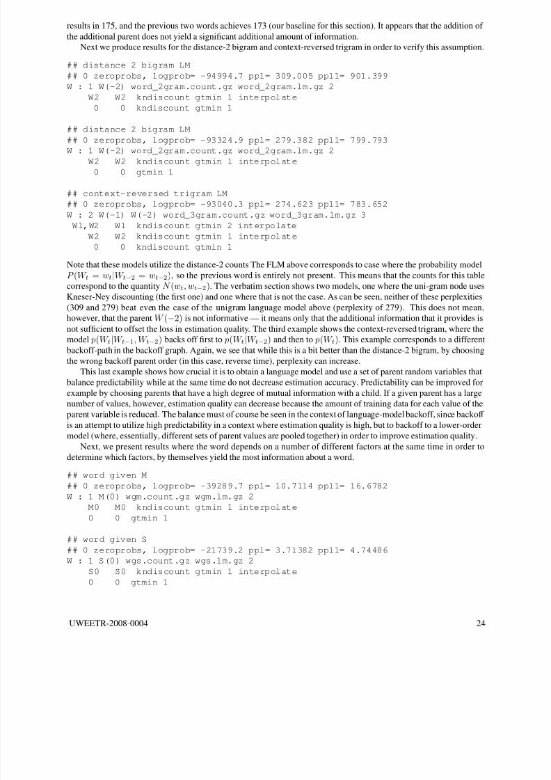
8/12/2019 Tutorial on Factored Language Models
http://slidepdf.com/reader/full/tutorial-on-factored-language-models 25/39
results in 175, and the previous two words achieves 173 (our baseline for this section). It appears that the addition of
the additional parent does not yield a significant additional amount of information.
Next we produce results for the distance-2 bigram and context-reversed trigram in order to verify this assumption.
## distance 2 bigram LM
## 0 zeroprobs, logprob= -94994.7 ppl= 309.005 ppl1= 901.399
W : 1 W(-2) word_2gram.count.gz word_2gram.lm.gz 2
W2 W2 kndiscount gtmin 1 interpolate
0 0 kndiscount gtmin 1
## distance 2 bigram LM
## 0 zeroprobs, logprob= -93324.9 ppl= 279.382 ppl1= 799.793
W : 1 W(-2) word_2gram.count.gz word_2gram.lm.gz 2
W2 W2 kndiscount gtmin 1 interpolate
0 0 gtmin 1
## context-reversed trigram LM
## 0 zeroprobs, logprob= -93040.3 ppl= 274.623 ppl1= 783.652
W : 2 W(-1) W(-2) word_3gram.count.gz word_3gram.lm.gz 3
W1,W2 W1 kndiscount gtmin 2 interpolate
W2 W2 kndiscount gtmin 1 interpolate
0 0 kndiscount gtmin 1
Note that these models utilize the distance-2 counts The FLM above corresponds to case where the probability model
P (W t = wt|W t−2 = wt−2), so the previous word is entirely not present. This means that the counts for this tablecorrespond to the quantity N (wt, wt−2). The verbatim section shows two models, one where the uni-gram node uses
Kneser-Ney discounting (the first one) and one where that is not the case. As can be seen, neither of these perplexities
(309 and 279) beat even the case of the unigram language model above (perplexity of 279). This does not mean,
however, that the parent W (−2) is not informative — it means only that the additional information that it provides is
not sufficient to offset the loss in estimation quality. The third example shows the context-reversed trigram, where the
model p(W t|W t−1, W t−2) backs off first to p(W t|W t−2) and then to p(W t). This example corresponds to a different
backoff-path in the backoff graph. Again, we see that while this is a bit better than the distance-2 bigram, by choosing
the wrong backoff parent order (in this case, reverse time), perplexity can increase.
This last example shows how crucial it is to obtain a language model and use a set of parent random variables that
balance predictability while at the same time do not decrease estimation accuracy. Predictability can be improved for
example by choosing parents that have a high degree of mutual information with a child. If a given parent has a large
number of values, however, estimation quality can decrease because the amount of training data for each value of the
parent variable is reduced. The balance must of course be seen in the context of language-model backoff, since backoff
is an attempt to utilize high predictability in a context where estimation quality is high, but to backoff to a lower-order
model (where, essentially, different sets of parent values are pooled together) in order to improve estimation quality.
Next, we present results where the word depends on a number of different factors at the same time in order to
determine which factors, by themselves yield the most information about a word.
## word given M
## 0 zeroprobs, logprob= -39289.7 ppl= 10.7114 ppl1= 16.6782
W : 1 M(0) wgm.count.gz wgm.lm.gz 2
M0 M0 kndiscount gtmin 1 interpolate
0 0 gtmin 1
## word given S
## 0 zeroprobs, logprob= -21739.2 ppl= 3.71382 ppl1= 4.74486
W : 1 S(0) wgs.count.gz wgs.lm.gz 2
S0 S0 kndiscount gtmin 1 interpolate
0 0 gtmin 1
UWEETR-2008-0004 24
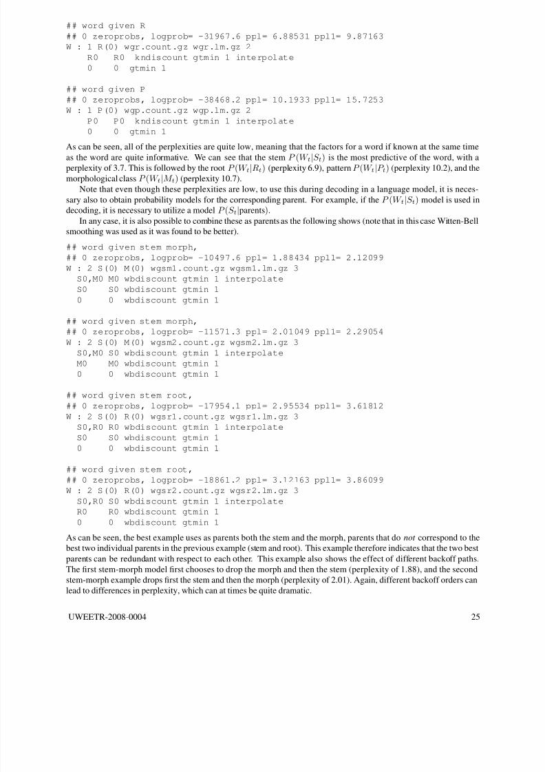
8/12/2019 Tutorial on Factored Language Models
http://slidepdf.com/reader/full/tutorial-on-factored-language-models 26/39
## word given R
## 0 zeroprobs, logprob= -31967.6 ppl= 6.88531 ppl1= 9.87163
W : 1 R(0) wgr.count.gz wgr.lm.gz 2
R0 R0 kndiscount gtmin 1 interpolate
0 0 gtmin 1
## word given P
## 0 zeroprobs, logprob= -38468.2 ppl= 10.1933 ppl1= 15.7253
W : 1 P(0) wgp.count.gz wgp.lm.gz 2
P0 P0 kndiscount gtmin 1 interpolate
0 0 gtmin 1As can be seen, all of the perplexities are quite low, meaning that the factors for a word if known at the same time
as the word are quite informative. We can see that the stem P (W t|S t) is the most predictive of the word, with a
perplexity of 3.7. This is followed by the root P (W t|Rt) (perplexity 6.9), pattern P (W t|P t) (perplexity 10.2), and the
morphological class P (W t|M t) (perplexity 10.7).
Note that even though these perplexities are low, to use this during decoding in a language model, it is neces-
sary also to obtain probability models for the corresponding parent. For example, if the P (W t|S t) model is used in
decoding, it is necessary to utilize a model P (S t|parents).
In any case, it is also possible to combine these as parents as the following shows (note that in this case Witten-Bell
smoothing was used as it was found to be better).
## word given stem morph,
## 0 zeroprobs, logprob= -10497.6 ppl= 1.88434 ppl1= 2.12099
W : 2 S(0) M(0) wgsm1.count.gz wgsm1.lm.gz 3S0,M0 M0 wbdiscount gtmin 1 interpolate
S0 S0 wbdiscount gtmin 1
0 0 wbdiscount gtmin 1
## word given stem morph,
## 0 zeroprobs, logprob= -11571.3 ppl= 2.01049 ppl1= 2.29054
W : 2 S(0) M(0) wgsm2.count.gz wgsm2.lm.gz 3
S0,M0 S0 wbdiscount gtmin 1 interpolate
M0 M0 wbdiscount gtmin 1
0 0 wbdiscount gtmin 1
## word given stem root,
## 0 zeroprobs, logprob= -17954.1 ppl= 2.95534 ppl1= 3.61812W : 2 S(0) R(0) wgsr1.count.gz wgsr1.lm.gz 3
S0,R0 R0 wbdiscount gtmin 1 interpolate
S0 S0 wbdiscount gtmin 1
0 0 wbdiscount gtmin 1
## word given stem root,
## 0 zeroprobs, logprob= -18861.2 ppl= 3.12163 ppl1= 3.86099
W : 2 S(0) R(0) wgsr2.count.gz wgsr2.lm.gz 3
S0,R0 S0 wbdiscount gtmin 1 interpolate
R0 R0 wbdiscount gtmin 1
0 0 wbdiscount gtmin 1
As can be seen, the best example uses as parents both the stem and the morph, parents that do not correspond to thebest two individual parents in the previous example (stem and root). This example therefore indicates that the two best
parents can be redundant with respect to each other. This example also shows the effect of different backoff paths.
The first stem-morph model first chooses to drop the morph and then the stem (perplexity of 1.88), and the second
stem-morph example drops first the stem and then the morph (perplexity of 2.01). Again, different backoff orders can
lead to differences in perplexity, which can at times be quite dramatic.
UWEETR-2008-0004 25
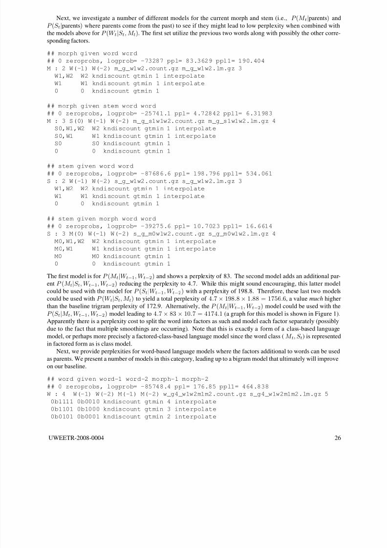
8/12/2019 Tutorial on Factored Language Models
http://slidepdf.com/reader/full/tutorial-on-factored-language-models 27/39
Next, we investigate a number of different models for the current morph and stem (i.e., P (M t|parents) and
P (S t|parents) where parents come from the past) to see if they might lead to low perplexity when combined with
the models above for P (W t|S t, M t). The first set utilize the previous two words along with possibly the other corre-
sponding factors.
## morph given word word
## 0 zeroprobs, logprob= -73287 ppl= 83.3629 ppl1= 190.404
M : 2 W(-1) W(-2) m_g_w1w2.count.gz m_g_w1w2.lm.gz 3
W1,W2 W2 kndiscount gtmin 1 interpolate
W1 W1 kndiscount gtmin 1 interpolate
0 0 kndiscount gtmin 1
## morph given stem word word
## 0 zeroprobs, logprob= -25741.1 ppl= 4.72842 ppl1= 6.31983
M : 3 S(0) W(-1) W(-2) m_g_s1w1w2.count.gz m_g_s1w1w2.lm.gz 4
S0,W1,W2 W2 kndiscount gtmin 1 interpolate
S0,W1 W1 kndiscount gtmin 1 interpolate
S0 S0 kndiscount gtmin 1
0 0 kndiscount gtmin 1
## stem given word word
## 0 zeroprobs, logprob= -87686.6 ppl= 198.796 ppl1= 534.061
S : 2 W(-1) W(-2) s_g_w1w2.count.gz s_g_w1w2.lm.gz 3
W1,W2 W2 kndiscount gtmin 1 interpolate
W1 W1 kndiscount gtmin 1 interpolate
0 0 kndiscount gtmin 1
## stem given morph word word
## 0 zeroprobs, logprob= -39275.6 ppl= 10.7023 ppl1= 16.6614
S : 3 M(0) W(-1) W(-2) s_g_m0w1w2.count.gz s_g_m0w1w2.lm.gz 4
M0,W1,W2 W2 kndiscount gtmin 1 interpolate
M0,W1 W1 kndiscount gtmin 1 interpolate
M0 M0 kndiscount gtmin 1
0 0 kndiscount gtmin 1
The first model is for P (M t|W t−1, W t−2) and shows a perplexity of 83. The second model adds an additional par-
ent P (M t|S t, W t−1, W t−2) reducing the perplexity to 4.7. While this might sound encouraging, this latter model
could be used with the model for P (S t|W t−1, W t−2) with a perplexity of 198.8. Therefore, these last two models
could be used with P (W t|S t, M t) to yield a total perplexity of 4.7 × 198.8 × 1.88 = 1756.6, a value much higher
than the baseline trigram perplexity of 172.9. Alternatively, the P (M t|W t−1, W t−2) model could be used with the
P (S t|M t, W t−1, W t−2) model leading to 4.7 × 83 × 10.7 = 4174.1 (a graph for this model is shown in Figure 1).
Apparently there is a perplexity cost to split the word into factors as such and model each factor separately (possibly
due to the fact that multiple smoothings are occurring). Note that this is exactly a form of a class-based language
model, or perhaps more precisely a factored-class-based language model since the word class ( M t, S t) is represented
in factored form as is class model.
Next, we provide perplexities for word-based language models where the factors additional to words can be used
as parents. We present a number of models in this category, leading up to a bigram model that ultimately will improve
on our baseline.
## word given word-1 word-2 morph-1 morph-2
## 0 zeroprobs, logprob= -85748.4 ppl= 176.85 ppl1= 464.838
W : 4 W(-1) W(-2) M(-1) M(-2) w_g4_w1w2m1m2.count.gz s_g4_w1w2m1m2.lm.gz 5
0b1111 0b0010 kndiscount gtmin 4 interpolate
0b1101 0b1000 kndiscount gtmin 3 interpolate
0b0101 0b0001 kndiscount gtmin 2 interpolate
UWEETR-2008-0004 26
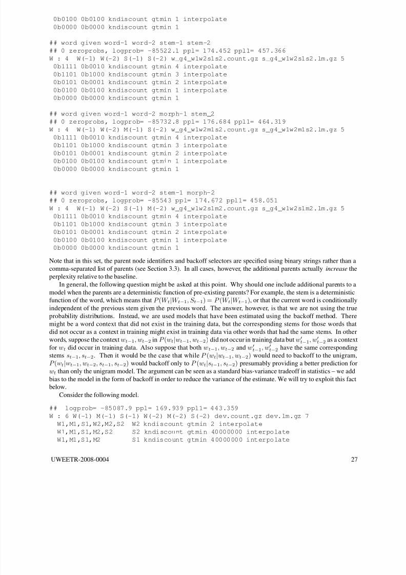
8/12/2019 Tutorial on Factored Language Models
http://slidepdf.com/reader/full/tutorial-on-factored-language-models 28/39
0b0100 0b0100 kndiscount gtmin 1 interpolate
0b0000 0b0000 kndiscount gtmin 1
## word given word-1 word-2 stem-1 stem-2
## 0 zeroprobs, logprob= -85522.1 ppl= 174.452 ppl1= 457.366
W : 4 W(-1) W(-2) S(-1) S(-2) w_g4_w1w2s1s2.count.gz s_g4_w1w2s1s2.lm.gz 5
0b1111 0b0010 kndiscount gtmin 4 interpolate
0b1101 0b1000 kndiscount gtmin 3 interpolate
0b0101 0b0001 kndiscount gtmin 2 interpolate
0b0100 0b0100 kndiscount gtmin 1 interpolate
0b0000 0b0000 kndiscount gtmin 1
## word given word-1 word-2 morph-1 stem_2
## 0 zeroprobs, logprob= -85732.8 ppl= 176.684 ppl1= 464.319
W : 4 W(-1) W(-2) M(-1) S(-2) w_g4_w1w2m1s2.count.gz s_g4_w1w2m1s2.lm.gz 5
0b1111 0b0010 kndiscount gtmin 4 interpolate
0b1101 0b1000 kndiscount gtmin 3 interpolate
0b0101 0b0001 kndiscount gtmin 2 interpolate
0b0100 0b0100 kndiscount gtmin 1 interpolate
0b0000 0b0000 kndiscount gtmin 1
## word given word-1 word-2 stem-1 morph-2
## 0 zeroprobs, logprob= -85543 ppl= 174.672 ppl1= 458.051W : 4 W(-1) W(-2) S(-1) M(-2) w_g4_w1w2s1m2.count.gz s_g4_w1w2s1m2.lm.gz 5
0b1111 0b0010 kndiscount gtmin 4 interpolate
0b1101 0b1000 kndiscount gtmin 3 interpolate
0b0101 0b0001 kndiscount gtmin 2 interpolate
0b0100 0b0100 kndiscount gtmin 1 interpolate
0b0000 0b0000 kndiscount gtmin 1
Note that in this set, the parent node identifiers and backoff selectors are specified using binary strings rather than a
comma-separated list of parents (see Section 3.3). In all cases, however, the additional parents actually increase the
perplexity relative to the baseline.
In general, the following question might be asked at this point. Why should one include additional parents to a
model when the parents are a deterministic function of pre-existing parents? For example, the stem is a deterministic
function of the word, which means that P (W t|W t−1, S t−1) = P (W t|W t−1), or that the current word is conditionallyindependent of the previous stem given the previous word. The answer, however, is that we are not using the true
probability distributions. Instead, we are used models that have been estimated using the backoff method. There
might be a word context that did not exist in the training data, but the corresponding stems for those words that
did not occur as a context in training might exist in training data via other words that had the same stems. In other
words, suppose the context wt−1, wt−2 in P (wt|wt−1, wt−2) did not occur in training data but wt−1, w
t−2 as a context
for wt did occur in training data. Also suppose that both wt−1, wt−2 and wt−1, w
t−2 have the same corresponding
stems st−1, st−2. Then it would be the case that while P (wt|wt−1, wt−2) would need to backoff to the unigram,
P (wt|wt−1, wt−2, st−1, st−2) would backoff only to P (wt|st−1, st−2) presumably providing a better prediction for
wt than only the unigram model. The argument can be seen as a standard bias-variance tradeoff in statistics – we add
bias to the model in the form of backoff in order to reduce the variance of the estimate. We will try to exploit this fact
below.
Consider the following model.
## logprob= -85087.9 ppl= 169.939 ppl1= 443.359
W : 6 W(-1) M(-1) S(-1) W(-2) M(-2) S(-2) dev.count.gz dev.lm.gz 7
W1,M1,S1,W2,M2,S2 W2 kndiscount gtmin 2 interpolate
W1,M1,S1,M2,S2 S2 kndiscount gtmin 40000000 interpolate
W1,M1,S1,M2 S1 kndiscount gtmin 40000000 interpolate
UWEETR-2008-0004 27
8/12/2019 Tutorial on Factored Language Models
http://slidepdf.com/reader/full/tutorial-on-factored-language-models 29/39
W1,M1,M2 M2 kndiscount gtmin 40000000 interpolate
W1,M1 W1 kndiscount gtmin 1 interpolate kn-count-parent 0b111111
M1 M1 kndiscount gtmin 3
0 0 kndiscount gtmin 1 kn-count-parent W1,M1
This model can be seen to improve on our baseline perplexity by a small amount. The model first attempts to utilize the
entire context — since both stems and morphs are deterministic functions of words, the context W1,M1,S1,W2,M2,S2
is identical to that of W1,W2. If that context does not exist in the training data (with a count of 2 or more), we drop the
parents W2, W2, and S1 (via very large min-counts as described in Section 3.3) and “land” on node W1,M1. This node
is attempted and used if a hit occurs, and otherwise the previous word is dropped, moving down until the unigram.
The next example improves on this as follows.
## logprob= -84924.5 ppl= 168.271 ppl1= 438.201
W : 6 W(-1) W(-2) M(-1) S(-1) M(-2) S(-2) dev.count.gz dev.lm.gz 9
W1,W2,M1,S1,M2,S2 W2 kndiscount gtmin 3 interpolate
W1,M1,S1,M2,S2 S2,M2 kndiscount gtmin 10000000 combine mean
W1,M1,S1,M2 M2 kndiscount gtmin 4 kn-count-parent 0b111111
W1,M1,S1,S2 S2 kndiscount gtmin 2 kn-count-parent 0b111111
W1,M1,S1 W1 kndiscount gtmin 2 interpolate
M1,S1 S1,M1 kndiscount gtmin 100000000 combine mean
M1 M1 kndiscount gtmin 3 kn-count-parent W1,M1,S1
S1 S1 kndiscount gtmin 1 kn-count-parent W1,M1,S1
0 0 kndiscount gtmin 1 kn-count-parent W1,M1,S1
This example first uses the complete context, and if a hit does not occur drops the parent W2. The next node
W1,M1,S1,M2,S2 uses generalized backoff to take a mean between the lower nodes where the parents S2 or M2
have been dropped. Each of these nodes are tried, and they respectively drop either M2 or S2, meaning they both
backoff to the same model W1,M1,S1. This node is attempted, and if a hit does not occur parent W1 is dropped. Then
at node M1,S1 generalized backoff is used again backing off to the mean of model M1 or S1, and then finally ending
up at the unigram. The perplexity achieved is 168.
The next trigram improves upon this even further.
## logprob= -84771.4 ppl= 166.724 ppl1= 433.423
W : 6 W(-1) W(-2) M(-1) S(-1) M(-2) S(-2) dev.count.gz dev.lm.gz 9
W1,W2,M1,S1,M2,S2 W2 kndiscount gtmin 3 interpolate
W1,M1,S1,M2,S2 S2,M2 kndiscount gtmin 10000000 combine mean
W1,M1,S1,M2 M2 kndiscount gtmin 4 kn-count-parent 0b111111
W1,M1,S1,S2 S2 kndiscount gtmin 2 kn-count-parent 0b111111
W1,M1,S1 W1 kndiscount gtmin 2 interpolate
M1,S1 S1,M1 kndiscount gtmin 100000000 combine max strategy bog_node_prob
M1 M1 kndiscount gtmin 3 kn-count-parent W1,M1,S1
S1 S1 kndiscount gtmin 1 kn-count-parent W1,M1,S1
0 0 kndiscount gtmin 1 kn-count-parent W1,M1,S1
This example is identical to the one above, except that rather than using mean combination at node M1,S1, max
combination is used. As can be seen the resulting perplexity achieved is 166.7.
This last example improves on this a bit more, but with a simpler model.
## Best perplexity found
## logprob= -84709 ppl= 166.097 ppl1= 431.488
W : 4 W(-1) W(-2) M(-1) S(-1) w_g_w1w2m1s1.count.gz w_g_w1w2m1s1.lm.gz 6
W1,W2,M1,S1 W2 kndiscount gtmin 3 interpolateW1,M1,S1 W1 kndiscount gtmin 2 interpolate
M1,S1 S1,M1 kndiscount gtmin 100000000 combine max strategy bog_node_prob
M1 M1 kndiscount gtmin 3 kn-count-parent W1,M1,S1
S1 S1 kndiscount gtmin 1 kn-count-parent W1,M1,S1
0 0 kndiscount gtmin 1 kn-count-parent W1,M1,S1
UWEETR-2008-0004 28
8/12/2019 Tutorial on Factored Language Models
http://slidepdf.com/reader/full/tutorial-on-factored-language-models 30/39
In this case, we use a trigram but only add additional parents M1 and S1. The entire context is first attempted, removing
W2 and then W1 if hits do not occur. Then generalized backoff inspired from the above is used to finish off down to
the unigram. The perplexity achieved is 166, the best perplexity we achieved on this data with any model.
While we expected that it would be possible to produce significant additional perplexity reductions with these
trigram like models (trigram because they depend on nothing farther in the past than the two previous words or
deterministic functions of these two previous words), the model search space is very large. Due to the time limitations
of the 6-week workshop, we decided to investigate bigrams for the remainder of the time. As you recall, the baseline
bigram had a perplexity of 175, much higher than the 166.7 achieved above and certainly higher than the baseline
trigram (173).
The next example is our first bigram that beats the baseline trigram perplexity, achieving 171. It does this by condi-
tioning on both the previousmorph class and stem in addition to the word (so the model is for P (W t|W t−1, M t−1, S t−1),but also uses one of the generalized backoff methods, bog node prob combining using the maximum. It first at-
tempts to use a context consisting of the previous word (W1,M1,S1 which is equivalent to W1 since M1,S1 are
deterministic functions of W1). If there is no language-model hit at that level, it jumps directly down to either using a
context consisting of either only M1 or S1. It does this “jump”, however, via a node that takes the maximum probabil-
ity of these two contexts, via the large gtmin parameter (so the node itself does not ever contribute a real probability,
it just acts to combine lower-level backoff-graph nodes). Lastly, notice that kn-count-parent was used to specify
that the original node should be used to form the Kneser-Ney meta-counts (the default would have been to use node
M1,S1. It was found in general that specifying a kn-count-parent node that included the word variable had a
beneficial effect on perplexity, when the model was a word model (i.e., when W t was on the left of the conditioning
bar in P (W t|parents)).
## logprob= -85204.8 ppl= 171.142 ppl1= 447.086
W : 3 W(-1) M(-1) S(-1) dev.count.gz dev.lm.gz 5
W1,M1,S1 W1 kndiscount gtmin 1 interpolate
M1,S1 S1,M1 kndiscount gtmin 100000000 strategy bog_node_prob combine max
M1 M1 kndiscount gtmin 3 kn-count-parent W1,M1,S1
S1 S1 kndiscount gtmin 3 kn-count-parent W1,M1,S1
0 0 kndiscount gtmin 1 kn-count-parent W1,M1,S1
The next example shows an even simpler bigram that also improves upon the baseline bigram and almost matches
the baseline trigram. In this case, generalized backoff is not used. Rather, the word context is augmented with the
morph variable.
## bigram that gets as good as a trigram.
## logprob= -85379.6 ppl= 172.958 ppl1= 452.721
W : 2 W(-1) M(-1) w_g_w1m1.count.gz w_g_w1m1.lm.gz 3
W1,M1 W1 kndiscount gtmin 1 interpolateM1 M1 kndiscount gtmin 3
0 0 kndiscount gtmin 1 kn-count-parent W1,M1
The next several examples show that perplexity can depend on adjusting the gtmin parameter. In this case,
changing gtmin for nodes M1, S1, and for no-parents might lead either to perplexity increases or decreases as the
example shows.
## logprob= -85140 ppl= 170.474 ppl1= 445.015
W : 3 W(-1) M(-1) S(-1) dev.count.gz dev.lm.gz 5
W1,M1,S1 W1 kndiscount gtmin 1 interpolate
M1,S1 S1,M1 kndiscount gtmin 100000000 strategy bog_node_prob combine max
M1 M1 kndiscount gtmin 3 kn-count-parent W1,M1,S1
S1 S1 kndiscount gtmin 2 kn-count-parent W1,M1,S10 0 kndiscount gtmin 1 kn-count-parent W1,M1,S1
## logprob= -85296 ppl= 172.087 ppl1= 450.016
W : 3 W(-1) M(-1) S(-1) dev.count.gz dev.lm.gz 5
W1,M1,S1 W1 kndiscount gtmin 1 interpolate
UWEETR-2008-0004 29

8/12/2019 Tutorial on Factored Language Models
http://slidepdf.com/reader/full/tutorial-on-factored-language-models 31/39
M1,S1 S1,M1 kndiscount gtmin 100000000 strategy bog_node_prob combine max
M1 M1 kndiscount gtmin 1 kn-count-parent W1,M1,S1
S1 S1 kndiscount gtmin 1 kn-count-parent W1,M1,S1
0 0 kndiscount gtmin 1 kn-count-parent W1,M1,S1
## logprob= -85267.8 ppl= 171.794 ppl1= 449.109
W : 3 W(-1) M(-1) S(-1) dev.count.gz dev.lm.gz 5
W1,M1,S1 W1 kndiscount gtmin 1 interpolate
M1,S1 S1,M1 kndiscount gtmin 100000000 strategy bog_node_prob combine max
M1 M1 kndiscount gtmin 3 kn-count-parent W1,M1,S1 interpolate
S1 S1 kndiscount gtmin 2 kn-count-parent W1,M1,S1 interpolate0 0 kndiscount gtmin 1 kn-count-parent W1,M1,S1
## logprob= -85132.5 ppl= 170.396 ppl1= 444.776
W : 3 W(-1) M(-1) S(-1) dev.count.gz dev.lm.gz 5
W1,M1,S1 W1 kndiscount gtmin 1 interpolate
M1,S1 S1,M1 kndiscount gtmin 100000000 strategy bog_node_prob combine max
M1 M1 kndiscount gtmin 3 kn-count-parent W1,M1,S1
S1 S1 kndiscount gtmin 1 kn-count-parent W1,M1,S1
0 0 kndiscount gtmin 1 kn-count-parent W1,M1,S1
The next example next shows that by using a different combination method (the mean in this case) it is possible to
retain the perplexity improvement. This is particularly relevant because the mean combination rule does not lead to a
costly language model to evaluate as does some of the other combination procedures.
## logprob= -85129.9 ppl= 170.37 ppl1= 444.693
W : 3 W(-1) M(-1) S(-1) dev.count.gz dev.lm.gz 5
W1,M1,S1 W1 kndiscount gtmin 1 interpolate
M1,S1 S1,M1 kndiscount gtmin 100000000 strategy bog_node_prob combine mean
M1 M1 kndiscount gtmin 3 kn-count-parent W1,M1,S1
S1 S1 kndiscount gtmin 1 kn-count-parent W1,M1,S1
0 0 kndiscount gtmin 1 kn-count-parent W1,M1,S1
The following example shows that using a weighted mean, it is possible to achieve still better perplexity. In this
case, most of the weight is given to the M1 node rather than to the S1 node.
## logprob= -85066.8 ppl= 169.723 ppl1= 442.691
W : 3 W(-1) M(-1) S(-1) dev.count.gz dev.lm.gz 5
W1,M1,S1 W1 kndiscount gtmin 1 interpolateM1,S1 S1,M1 kndiscount gtmin 100000000 strategy bog_node_prob \
combine wmean M1 7 S1 3
M1 M1 kndiscount gtmin 3 kn-count-parent W1,M1,S1
S1 S1 kndiscount gtmin 1 kn-count-parent W1,M1,S1
0 0 kndiscount gtmin 1 kn-count-parent W1,M1,S1
Changing the strategy to counts prod card norm does not seem to show any appreciable change.
## logprob= -85187 ppl= 170.959 ppl1= 446.518
W : 3 W(-1) M(-1) S(-1) dev.count.gz dev.lm.gz 5
W1,M1,S1 W1 kndiscount gtmin 1 interpolate
M1,S1 S1,M1 kndiscount gtmin 100000000 \
strategy counts_prod_card_norm combine max
M1 M1 kndiscount gtmin 3 kn-count-parent W1,M1,S1S1 S1 kndiscount gtmin 1 kn-count-parent W1,M1,S1
0 0 kndiscount gtmin 1 kn-count-parent W1,M1,S1
Changing the strategy to counts sum counts norm and combiningmethod to gmean leads to a slight increase
in perplexity.
UWEETR-2008-0004 30
8/12/2019 Tutorial on Factored Language Models
http://slidepdf.com/reader/full/tutorial-on-factored-language-models 32/39
## logprob= -85252.5 ppl= 171.635 ppl1= 448.616
W : 3 W(-1) M(-1) S(-1) dev.count.gz dev.lm.gz 5
W1,M1,S1 W1 kndiscount gtmin 1 interpolate
M1,S1 S1,M1 kndiscount gtmin 100000000 \
strategy counts_sum_counts_norm combine gmean
M1 M1 kndiscount gtmin 3 kn-count-parent W1,M1,S1
S1 S1 kndiscount gtmin 1 kn-count-parent W1,M1,S1
0 0 kndiscount gtmin 1 kn-count-parent W1,M1,S1
## logprob= -85156.7 ppl= 170.646 ppl1= 445.548
W : 3 W(-1) M(-1) S(-1) dev.count.gz dev.lm.gz 5W1,M1,S1 W1 kndiscount gtmin 1 interpolate
M1,S1 S1,M1 kndiscount gtmin 100000000 strategy counts_sum_counts_norm \
combine mean
M1 M1 kndiscount gtmin 2 kn-count-parent W1,M1,S1
S1 S1 kndiscount gtmin 1 kn-count-parent W1,M1,S1
0 0 kndiscount gtmin 1 kn-count-parent W1,M1,S1
## logprob= -85150.3 ppl= 170.58 ppl1= 445.346
W : 3 W(-1) M(-1) S(-1) dev.count.gz dev.lm.gz 5
W1,M1,S1 W1 kndiscount gtmin 1 interpolate
M1,S1 S1,M1 kndiscount gtmin 100000000 strategy counts_sum_counts_norm \
combine mean
M1 M1 kndiscount gtmin 4 kn-count-parent W1,M1,S1S1 S1 kndiscount gtmin 1 kn-count-parent W1,M1,S1
0 0 kndiscount gtmin 1 kn-count-parent W1,M1,S1
Using a weighted mean with counts sum counts norm improves things a bit further.
## logprob= -84948.9 ppl= 168.519 ppl1= 438.966
W : 3 W(-1) M(-1) S(-1) dev.count.gz dev.lm.gz 5
W1,M1,S1 W1 kndiscount gtmin 2 interpolate
M1,S1 S1,M1 kndiscount gtmin 100000000 strategy counts_sum_counts_norm \
combine wmean M1 7 S1 3
M1 M1 kndiscount gtmin 3 kn-count-parent W1,M1,S1
S1 S1 kndiscount gtmin 1 kn-count-parent W1,M1,S1
0 0 kndiscount gtmin 1 kn-count-parent W1,M1,S1
Using the mean, however, produces a slight modification.
## logprob= -84967 ppl= 168.703 ppl1= 439.536
W : 3 W(-1) M(-1) S(-1) dev.count.gz dev.lm.gz 5
W1,M1,S1 W1 kndiscount gtmin 2 interpolate
M1,S1 S1,M1 kndiscount gtmin 100000000 combine mean
M1 M1 kndiscount gtmin 3 kn-count-parent W1,M1,S1
S1 S1 kndiscount gtmin 1 kn-count-parent W1,M1,S1
0 0 kndiscount gtmin 1 kn-count-parent W1,M1,S1
The last example shows our best bigram, achieving a perplexity of 167.4, which is not only better than the baseline
trigram, but is close to the much more expensive generalized-backoff trigram perplexity seen above.
## logprob= -84845.2 ppl= 167.468 ppl1= 435.719
W : 3 W(-1) M(-1) S(-1) dev.count.gz dev.lm.gz 5
W1,M1,S1 W1 kndiscount gtmin 2 interpolate
M1,S1 S1,M1 kndiscount gtmin 100000000 combine max strategy bog_node_prob
M1 M1 kndiscount gtmin 3 kn-count-parent W1,M1,S1
UWEETR-2008-0004 31
8/12/2019 Tutorial on Factored Language Models
http://slidepdf.com/reader/full/tutorial-on-factored-language-models 33/39
S1 S1 kndiscount gtmin 1 kn-count-parent W1,M1,S1
0 0 kndiscount gtmin 1 kn-count-parent W1,M1,S1
This model increases gtmin to 2 for the W1,M1,S1 node yielding the further improvements.
As can be seen, the space of possible models is quite large, and searching through such a model space by hand can
be quite time consuming. We expect that automatic data-driven structure learning procedures to produce these models
might yield improvements over the models above (all of which were derived and specified by-hand).
5 Data-driven Search of FLM Parameters
In order to use an FLM, three types of parameters need to specified: the initial conditioning factors, the backoff graph, and the smoothing options. The initial conditioning factors specifies which factors shall be used in estimating
n-gram probabilities (design issue 1 in Section 1.2). The backoff graph and smoothing options indicate the procedures
for robust estimation in the case of insufficient data (design issue 2). The goal of data-driven search is to find the
parameter combinations that create FLMs that achieve a low perplexity on unseen test data.
The resulting model space is extremely large: given a factored word representation with a total of k factors, there
arek
n=1
kn
possible subsets of initial conditioning factors. For a set of m conditioning factors, there are up to m!
backoff paths, each with its own smoothing options. Unless m is very small, exhaustive search is infeasible.
Moreover, nonlinear interactions between parametersmake it difficult to guide the search into a particulardirection.
For instance, a particular backoff path may work well with Kneser-Ney smoothing, while a slightly different path may
find poor performance using the same method. Good structures are ultimately dependent on the data, so parameter
sets that work well for one corpus cannot necessarily be expected to perform well on another.
We have developed an efficient search algorithm called GA-FLM for tuning FLMs. It is based on genetic algo-
rithms and takes as inputs a factored training text and a factored development text and attempts to find FLM parameters
that minimize perplexity on the development text. The code is publicly-available at
http://ssli.ee.washington.edu/people/duh/research/gaflm.html .
We recommend FLM users to use this GA procedure or other data-driven search methods if hand-tuning of FLMs be-
comes too time-consuming. In the following, we provide a brief description of the GA-FLM code. More information
is availabe in [7].
5.1 GA-FLM Code Overview
The general flow of the program is illustrated in Figure 8. First, we initialize a population of genes. Each gene repre-
sents an FLM with specific conditioning factors, backoff graph, and smoothing options. For each gene, we print out its
factor-file and from this factor-file we train and test the language model using the conventional fngram-count and
fngram tools in SRILM. The perplexity on the user-supplied development set is used to determine the fitness value
of the gene. After fitness evaluation, selection/crossover/mutation occurs and the next population of genes is ready
to be evaluated. The program runs until convergence or maximum generation specified by the user. Finally, “elitist”
selection is implemented, so the best gene of each generation is gauranteed a spot in the next generation. Refer to [7]
for details on how an FLM is encoded as a gene.
5.2 GA-FLM: General Requirements and Installation
Make sure you have the SRI Language Modeling Toolkit Version 1.4.1 or above. The two executables that are needed
in that package are ”fngram-count” and ”fngram”, which builds and tests factored language models, respectively. The
GA-FLM tool can be downloaded at:
http://ssli.ee.washington.edu/people/duh/research/gaflm.html
To install, simply download and unzip the tarball. Then type ”make” in the root directory. This will create an exe-
cutable ga-flm, as well as other supporting scripts.
UWEETR-2008-0004 32
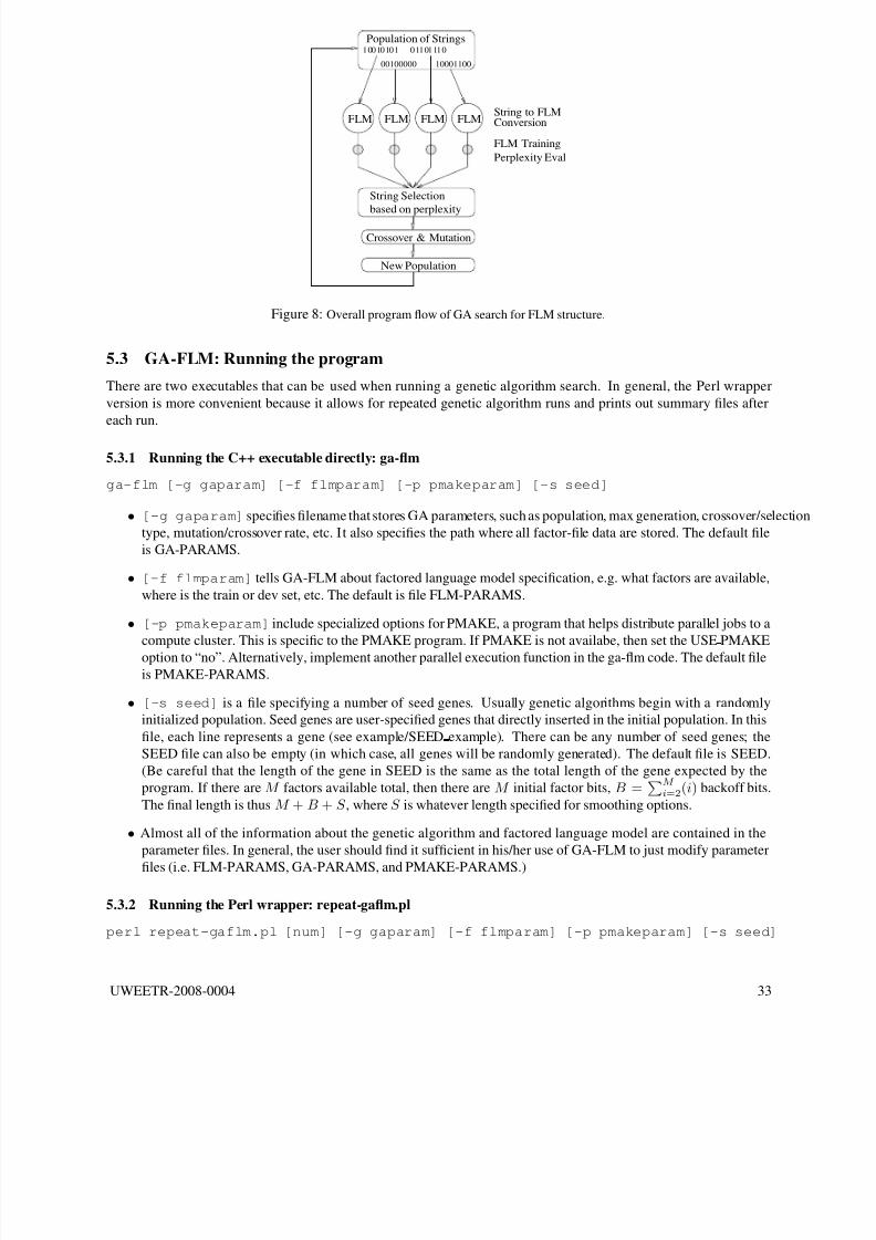
8/12/2019 Tutorial on Factored Language Models
http://slidepdf.com/reader/full/tutorial-on-factored-language-models 34/39
FLM FLMFLM FLM
Crossover & Mutation
New Population
10010101 01101110
1000110000100000
String to FLMConversion
FLM Training
Perplexity Eval
String Selection
based on perplexity
Population of Strings
Figure 8: Overall program flow of GA search for FLM structure.
5.3 GA-FLM: Running the program
There are two executables that can be used when running a genetic algorithm search. In general, the Perl wrapper
version is more convenient because it allows for repeated genetic algorithm runs and prints out summary files after
each run.
5.3.1 Running the C++ executable directly: ga-flm
ga-flm [-g gaparam] [-f flmparam] [-p pmakeparam] [-s seed]
• [-g gaparam] specifies filename that stores GA parameters, such as population, max generation, crossover/selection
type, mutation/crossover rate, etc. It also specifies the path where all factor-file data are stored. The default file
is GA-PARAMS.
• [-f flmparam] tells GA-FLM about factored language model specification, e.g. what factors are available,
where is the train or dev set, etc. The default is file FLM-PARAMS.
• [-p pmakeparam] include specialized options for PMAKE, a program that helps distribute parallel jobs to a
compute cluster. This is specific to the PMAKE program. If PMAKE is not availabe, then set the USE PMAKE
option to “no”. Alternatively, implement another parallel execution function in the ga-flm code. The default file
is PMAKE-PARAMS.
• [-s seed] is a file specifying a number of seed genes. Usually genetic algorithms begin with a randomly
initialized population. Seed genes are user-specified genes that directly inserted in the initial population. In this
file, each line represents a gene (see example/SEED example). There can be any number of seed genes; the
SEED file can also be empty (in which case, all genes will be randomly generated). The default file is SEED.
(Be careful that the length of the gene in SEED is the same as the total length of the gene expected by the
program. If there are M factors available total, then there are M initial factor bits, B = M
i=2(i) backoff bits.
The final length is thus M + B + S , where S is whatever length specified for smoothing options.
• Almost all of the information about the genetic algorithm and factored language model are contained in the
parameter files. In general, the user should find it sufficient in his/her use of GA-FLM to just modify parameter
files (i.e. FLM-PARAMS, GA-PARAMS, and PMAKE-PARAMS.)
5.3.2 Running the Perl wrapper: repeat-gaflm.pl
perl repeat-gaflm.pl [num] [-g gaparam] [-f flmparam] [-p pmakeparam] [-s seed]
UWEETR-2008-0004 33
8/12/2019 Tutorial on Factored Language Models
http://slidepdf.com/reader/full/tutorial-on-factored-language-models 35/39
• repeat-gaflm.pl is a Perl wrapper to ga-flm. There are two additions that make this Perl wrapper more
flexible:
• 1. The user can specify [num], which will call ga-flm repeatedly for [num] times. This is useful for when the
user wants to run several genetic algorithm experiments.
• 2. The Perl wrapper produces a “timelog” and a “summary” file, which summarizes the perplexity results
across the entire genetic algorithm run. This easy-to-read summary file is a convenient way to acquire the best
factor-files after a genetic algorithm run.
• The [g|f|p|s] parameters are simply passed on to ga-flm, and are therefore the same.
• The default for [num], when omitted, is 1.
5.4 Example runs of GA-FLM
The following two examples illustrates the use of GA-FLM to find factored language model structures. The data used
is the CoNLL 2002 shared task corpus. It is included in example/data/
5.4.1 Serial execution example
Try the following command:
perl repeat-gaflm.pl 2
This will run GA-FLM twice. No [g|f|p|s] options are given, so the defaults (e.g. GA-PARAMS, FLM-
PARAMS, PMAKE-PARAMS, SEED) are read. Note that PMAKE-PARAMS specifies USE PMAKE to “no”, which
in the current implementation implies serial execution for evaluating language model fitness. This may be a bit slow,but we have set the population and generation in GA-PARAMS to be small, so the GA-FLM should not take too long.
From GA-PARAMS, we know that the results are stored in example/serial. Go to that directory. You’ll find a
bunch of files:
• .flm files and .EvalLog files are the factor-file and perplexity file of a specific gene, respectively. The .flm
files are generated from transforming the gene sequence to a factored language model. The .EvalLog are
obtained after training the factored language model on the train-set and testing on the dev-set.
• The logfile files contain information about population fitness across generations.
• The summary file contains all the factor-files of the genes over the entire genetic algorithm run, together with
their corresponding perplexities. The end of the file contains a list of genes in descending order of perplexity.
• The .complexity files represents the number of parameters used by the factor file and is used by the BayesianInfo Criteria (BIC) fitness function. If the InversePPL fitness function is specified instead, these files are not
needed.
5.4.2 Parallel Pmake execution example
Genetic algorithms are very suited to parallel processing. The building and testing of each factored language model can
be done independently at parallel machines, and no communication between machines are needed. Try the following
command if you have the PMAKE parallel jobs distribution program available:
perl repeat-gaflm.pl -g example/GA-PARAMS-parallel -p example/PMAKE-PARAMS-paralle
Note that we have only changed the GA-PARAMS and PMAKE-PARAMS files. Specifically, the PMAKE-
PARAMS file now tells GA-FLM to use parallel processing. The GA-PARAMS file specifies the results to be stored
in example/parallel.
If you do not have PMAKE, you should implement an interface to whatever parallel processing program exist onyour computer system. (Serial processing is inherently slow and not recommended; it is included in this package only
for demonstration and debugging purposes). See Section 5.5.3 for instructions on how to do this.
UWEETR-2008-0004 34

8/12/2019 Tutorial on Factored Language Models
http://slidepdf.com/reader/full/tutorial-on-factored-language-models 36/39
5.5 GA-FLM Parameters Files
There are three parameter files read in by ga-flm. They allow the user to specific the particular GA options or FLM
options to use in the search. In the following we shall explain each parameter file in detail.
5.5.1 GA-PARAMS File
Here is an example GA-PARAMS file:
Population Size = 4
Maximum no of generations = 2
P(Crossover) = 0.9
P(Mutation) = 0.01
Crossover type = 2-point
Selection type = SUS
(tournament selection) n = 3
Fitness scaling constant = 1000000
Fitness function = BIC
BIC constant k = 1.0
PATH for GA FLM files = example/serial/
All the above parameters are quite useful to the general user. They can be divided into three groups.
Genetic algorithm operators
The first 5 parameters are standard parameters to genetic algorithm. Usually, to find good factored language models,
one needs to experiment with several different crossover/selection/mutation and population sizes. In more detail:
• Crossover type may be {2-point,1-point,uniform}
• Selection type may be {SUS, roulette, tournament}
• (tournament selection) n is the number of genes picked in tournament selection
Fitness function
The following 3 parameters define the fitness function:
• Fitness scaling constant is a linear scaling constant that makes sure fitness values are in reasonable ranges. Make
this very high if you want a high convergence threshold (genetic algorithm stops quicker), or lower if you want
to fine-tune the last generations.
• Fitness function is currently {BIC,inversePPL}, two different methods to evaluate fitness of a language model.
• BIC k can be any float number. It is used as the Bayesian Info Criteria weight for complexity penalty. It is
ignored when inversePPL is selected as fitness function.
The inversePPL fitness function is implemented as:
fitnessinversePPL = c ∗ ( 1
perplexity) (1)
where c is the fitness scaling constant.
The BIC fitness function is implemented as:
fitnessBIC = c ∗ (−logprobability + k
2 ∗ log(N )) (2)
UWEETR-2008-0004 35

8/12/2019 Tutorial on Factored Language Models
http://slidepdf.com/reader/full/tutorial-on-factored-language-models 37/39
where c is the fitness scaling constant, k is the weighting for logprobability vs. complexity penality, and N is the
number of parameters used by the factored language model under evaluation. ( N is the total number of n-gram types
for the factored language model, which is taken from the .complexity file).
You may wish to implement your own fitness function. To do so, hack the following part of the code:
ga-flm.cc::collectPPL().
Add your own fitness function after the BIC and inversePPL fitness functions. The quantities “logprob”, “com-
plexity”, and “ppl” (perplexity) are available for fitness computation. Your fitness function may also need some
input specified through parameter files. In that case, add some code to the “READ GA-PARAMS FILE” portion of
ga-flm.cc::initialize(void). Refer to the “BIC k value” implementation there for an example.
Path for GA-FLM files
• PATH for GA FLM files is where all the EvalLog, ga.pmake, and factor-files are stored
5.5.2 FLM-PARAMS File
Here is an example FLM-PARAMS File:
Data Path = example/data/
TrainSet = wsj 20 train.factored.txt
DevSet = wsj 20 dev.factored.txt
fngram-count Path = fngram-count
fngram Path = fngramfngram-count Options = ””
fngram Options = ””
Factor to Predict = W
Total Available Factors = W,P,C
Context of Factors = 1,2
Smoothing Options Length = 16
Discount Options = kndiscount, cdiscount 1,wbdiscount, ndiscount
Default Discount = wbdiscount
Max cutoff (max gtmin) = 5
The above parameters relate to the factored language model training/testing and can be divided into 3 general
sections: parameters regarding data, parameters regarding the SRI Language Modeling program, and parameters
regarding the factored language model specification:
Data location
• Data Path is the directory path for both training and dev sets.
• TrainSet and DevSet are the filenames of the training and dev set. These files are the factored textfiles as-
sumed by the SRILM fngram programs. (e.g. The sentences are composed of factored bundles like W-
word:P:pos:C:chunk). See example/data for examples.
SRI Language Modeling program options
• FngramCount Path and Fngram Path are the paths of the fngram-count and fngram files, respectively.
• FngramCount options and Fngram options may contain any command-line options for training/testing the lan-guage model. These options are passed directly to fngram-count and fngram. For example,
FngramCount options = ”-unk”
If no options are needed, use FngramCount options = ”” (with the quotes)
UWEETR-2008-0004 36

8/12/2019 Tutorial on Factored Language Models
http://slidepdf.com/reader/full/tutorial-on-factored-language-models 38/39
Factored Language Model Specifications
• Factor to Predict is the factor we wish to predict through the language model. Usually, this is W (word), but
may be any factor.
• Total Available Factors and Context of Factors together specify the tags of factors that will be used in the GA
optimization. There are two ways to specify these two parameters:
1. Specify both factors and context desired, e.g.
Total Available Factors = W,S,P
Context = 1,2
= You’ll get factors W(-1),S(-1),P(-1),W(-2),S(-2),P(-2).
2. Specify factor-tags directly without specifying context,e.g.Total Available Factors = W1,S1,P1,W2,S2,P2
Context = 0
= Note that in this case, you must set context=0.
The advantage of method 1 is that there’s less typing to do. The advantage of method 2 is that you
can specify arbitrary factor combinations. For example, you can specify W1,S1,S2 which is not possible with
method 1.
Be sure that the tags and numbers for context are separated by commas (,) as that is the delimiter that
signals the program how to tell the tags apart.
• Smoothing Options Length is the number of smoothing option parameters. This defines the length of the
smoothing options gene. Since smoothing is defined as tuples of (discount,gtmin), this should be any even
number {0,2,4,...}. If you believe smoothing options are important in the optimization, make this gene long.
• Discount options can be any of the usual fngramdiscounting options (e.g. kndiscount,ukndiscount,wbdiscount,cdiscount
1,kndiscount). Like the Total Available Factors, be sure to use commas to delimit discounting options. Any
number of discounting options may be used.
• Default Discount is the one used for unigram and other cases when there are more backoff edges to smooth than
number of smoothing options specified in Smoothing Options Length.
• Max Cutoff indicates the max possible value for gtmin. gtmin is the min cutoff count for a ngram to be included
in the language model estimation.
5.5.3 PMAKE-PARAMS File
Here is an example of the PMAKE-PARAMS file:
Use Pmake? = yesNum Pmake Jobs = 20
Scratch Space to Use = example/parallel/
Export Attributes = Linux !1000RAM !2000RAM
• Use Pmake = {yes,no}. Current implementation can evaluate FLMs serially or parallelly using Pmake. Enter
yes here if Pmake is available. Otherwise, enter no to use serial or adapt the code to your own parallel processing
platform.
• Num Pmake Jobs is the max number of pmake jobs (e.g. -J option in pmake)
• Scratch space is the place for storing big language model files, count files, and train/dev set data. In the Pmake
implementation, all these files are stored locally in the scratch space of each computer. They are deleted aftereach fitness evaluation.
• Export attributes are the Pmake export attributes. (e.g. Linux !1000RAM !2000RAM).
UWEETR-2008-0004 37

8/12/2019 Tutorial on Factored Language Models
http://slidepdf.com/reader/full/tutorial-on-factored-language-models 39/39
You may wish to implement your own parallel execution code. To do so, hack the following part of the code:
ga-flm.cc::executeFngramCommands(fngramCommands) .
The fngramCommands is a queue object containing a list of commands for all genes that need to be evalu-
ated in this generation. These commands are independent, and can therefore be executed in parallel without any
mutual communication. As long as you ensure that all commands in fngramCommands are executed before
ga-flm.cc::executeFngramCommands(fngramCommands) exits, then GA-FLM will work fine. Refer
to the serial execution and the executeFngramCommandsByPmake(fngramCommands) for example imple-
mentations.
After implementing this code, be sure to modify the USE PMAKE variable and the PMAKE-PARAMS file so you
can tell GA-FLM which execution mode you desire.
References
[1] A. L. Berger, S.A. Della Pietra, and V.J. Della Pietra. A maximum entropy approach to natural language pro-
cessing. Computational Linguistics, 22(1):39–71, 1996.
[2] J. Bilmes and G. Zweig. The Graphical Models Toolkit: An open source software system for speech and time-
series processing. Proc. IEEE Intl. Conf. on Acoustics, Speech, and Signal Processing, 2002.
[3] J. A. Bilmes. Graphical models and automatic speech recognition. In R. Rosenfeld, M. Ostendorf, S. Khudanpur,
and M. Johnson, editors, Mathematical Foundations of Speech and Language Processing. Springer-Verlag, New
York, 2003.
[4] Jeff A. Bilmes and Katrin Kirchhoff. Factored language models and generalized parallel backoff. In Proceedings
of HLT/NAACL, pages 4–6, 2003.
[5] S. F. Chen and J. Goodman. An empirical study of smoothing techniques for language modeling. In Arivind
Joshi and Martha Palmer, editors, Proceedings of the Thirty-Fourth Annual Meeting of the Association for Com-
putational Linguistics, pages 310–318, San Francisco, 1996. Association for Computational Linguistics, Morgan
Kaufmann Publishers.
[6] S. F. Chen and J. Goodman. An empirical study of smoothing techniques for language modeling. Technical
Report Tr-10-98, Center for Research in Computing Technology, Harvard University, Cambridge, Massachusetts,
August 1998.
[7] Kevin Duh and Katrin Kirchhoff. Automatic learning of language model structure. In Proceedings of the Inter-
national Conference on Computational Linguistics (COLING), 2004.
[8] N. Friedman and D. Koller. Learning Bayesian networks from data. In NIPS 2001 Tutorial Notes. Neural
Information Processing Systems, Vancouver, B.C. Canada, 2001.
[9] F. Jelinek. Statistical Methods for Speech Recognition. MIT Press, 1997.
[10] K. Kirchhoff et al. Novel speech recognition models for arabic: JHU 2002 summer workshop final report, 2002.
[11] S.L. Lauritzen. Graphical Models. Oxford Science Publications, 1996.
[12] A. Stolcke. SRILM- an extensible language modeling toolkit. In Proc. Int. Conf. on SpokenLanguage Processing,
Denver, Colorado, September 2002.
[13] E.W.D. Whittaker and P.C. Woodland. Particle-based language modeling. In Proc. Int. Conf. on Spoken Language
Processing, Beijing, China, 2000.
UWEETR-2008-0004 38