Embed Size (px)
Citation preview

Design and Analysis of Corrugated Conical
Horn Antennas with Terahertz Applications
Presented by
Fiachra Cahill, B.Sc
A thesis submitted for the degree of
Master of Science
Department of Experimental Physics Maynooth University, NUI Maynooth
Co. Kildare Ireland
September 2015
Head of Department
Professor J. A. Murphy, M.Sc., M.S., Ph.D.
Research Supervisor
Dr Créidhe O’ Sullivan, Ph.D.

i
Table of Contents
Abstract........................................................................................................................ v
Acknowledgements ..................................................................................................... vi
1. Introduction ......................................................................................................... 1
1.1 Introduction to THz radiation ........................................................................ 1
1.2 Applications of THz radiation ........................................................................ 2
1.2.1 Astronomical applications. ..................................................................... 2
1.2.2 Commercial applications ........................................................................ 4
1.3 SWISSto12® ................................................................................................... 5
1.4 Outline of thesis ............................................................................................ 9
2. Introduction to waveguides ............................................................................... 12
2.1 Circular waveguides..................................................................................... 12
2.1.1 Derivation of electric and magnetic fields in a circular waveguide ..... 13
2.1.2 Circular waveguide modes ................................................................... 16
2.1.3 Mode characteristics ............................................................................ 17
2.2 Rectangular waveguides .............................................................................. 20
2.3 Corrugated cylindrical waveguides & horn antennas ................................. 23
2.3.1 Waveguides as antennas ...................................................................... 23
2.3.2 Hybrid modes ....................................................................................... 24
2.3.3 Corrugated waveguides ....................................................................... 28
2.4 Summary ...................................................................................................... 29
3. Conical horn analysis methods .......................................................................... 30
3.1 The surface impedance model .................................................................... 30
3.1.1 Hybrid mode analysis ........................................................................... 31
3.2 Mode matching: SCATTER ........................................................................... 35
3.2.1 Mode normalisation and conversion to Cartesian coordinates .......... 36

ii
3.2.2 Scattering matrix formalisation ........................................................... 38
3.2.3 Mode scattering along a uniform section of waveguide ..................... 41
3.2.4 Mode scattering at a waveguide discontinuity .................................... 41
3.2.5 SCATTER algorithm. .............................................................................. 44
3.2.6 Radiation patterns ................................................................................ 46
3.3 Finite Integration Technique, CST: Microwave Studio ................................ 47
3.3.1 Solver Types ......................................................................................... 48
3.3.2 Setting up a simulation ........................................................................ 48
3.3.3 Field monitors ...................................................................................... 52
3.4 Comparison of SCATTER and CST ................................................................ 53
3.5 Summary ...................................................................................................... 55
4. Designing corrugated conical horn antennas .................................................... 57
4.1 System design requirements ....................................................................... 57
4.1.1 Design goals.......................................................................................... 59
4.2 Rectangular to circular transition ................................................................ 59
4.2.1 Two step transition .............................................................................. 61
4.2.2 Tapered transition ................................................................................ 64
4.3 Circular waveguide to corrugated horn transition ...................................... 66
4.3.1 Claricoats throat ................................................................................... 66
4.3.2 Zhang throat ......................................................................................... 70
4.4 Throat to aperture transition ...................................................................... 74
4.5 Use of SCATTER in design process ............................................................... 78
4.6 Full design procedure .................................................................................. 80
4.6.1 Design parameters ............................................................................... 80
4.6.2 Performance metrics ............................................................................ 82
4.7 Example of a design (WR-1.0) ..................................................................... 84

iii
4.8 Results ......................................................................................................... 92
4.8.1 WR-1.0 .................................................................................................. 93
4.8.2 WR-1.5 .................................................................................................. 93
4.8.3 WR-3.4 .................................................................................................. 94
4.8.4 WR-3.4 EPFL ......................................................................................... 94
4.8.5 WR-5.1 .................................................................................................. 96
4.8.6 WR-6.5 .................................................................................................. 96
4.8.7 WR-10 ................................................................................................... 98
4.8.8 Final performance curves ..................................................................... 98
4.8.9 WR+ bands (WR-6.5+, WR-10+) ......................................................... 100
4.8.10 Analysis of optimised geometries ...................................................... 101
4.9 Tolerance analysis ..................................................................................... 103
4.9.1 WR-1.0 ................................................................................................ 104
4.9.2 WR-6.5 ................................................................................................ 105
4.9.3 WR-10 ................................................................................................. 106
4.10 Conclusions ............................................................................................ 107
5. Measurements of WR-1.5 and WR-6.5 modules ............................................. 110
5.1 The vector network analyser ..................................................................... 110
5.2 WR-1.5 module measurements ................................................................ 112
5.3 WR-6.5 module measurements ................................................................ 117
5.3.1 WR-6.5 return loss ............................................................................. 117
5.3.2 WR-6.5 insertion loss ......................................................................... 118
5.3.3 Time-gating ........................................................................................ 119
5.4 Conclusions ................................................................................................ 123
6. Final summary and conclusion ......................................................................... 125
6.1 Future work ............................................................................................... 127

iv
7. Bibliography ..................................................................................................... 129
8. Appendix A ....................................................................................................... 133

v
Abstract
The focus of this thesis is the design and analysis of corrugated conical horn
antennas for use in the THz region of the electromagnetic spectrum, for the
company SWISSto12®. These antennas are designed to work across the industry
standard WR frequency bands, as free-space radiators or as part of a larger
quasi-optical network. The main analysis tools used in this work were the in-house
mode-matching code, SCATTER, and the commercially available
CST: Microwave Studio, which makes use of the finite integration technique. A
version of SCATTER which incorporated creation of a corrugated horn antenna’s
geometry from user chosen inputs was used to perform parametric sweep analysis
when designing the horn antennas. The main design stages were (1) a rectangular
to circular transition from a WR rectangular waveguide to a circular waveguide
input, (2) a circular smooth-walled to corrugated transition and (3) a transition from
a small diameter corrugated waveguide to either a large diameter corrugated
waveguide or to free-space. Several styles were examined for the various design
stages; the choice of style for the final designs was influenced not only by their
performance but also by manufacturing feasibility and cost. Overall, nine individual
designs for the WR-1.0. WR-1.5, WR-3.4, WR-5.1, WR-6.5, WR-6.5+, WR-10 and
WR-10+ bands have been completed to meet the criteria set by SWISSto12; two of
these designs have been manufactured and tested and the results from the
measurements performed are presented here.

vi
Acknowledgements
First of all I must thank my supervisor Dr Créidhe O’ Sullivan for her constant
support and encouragement and for her many kind words over the past two years. I
also need to especially mention Dr Stephen Doherty for his mentorship and
guidance and for organizing my funding from SWISSto12, without which this thesis
may have been very different. I would like to thank all of the other senior members
of the Terahertz group: Dr J. Anthony Murphy, Dr Marcin Gradziel and
Dr Neil Trappe who have all helped me out in one way or another during course of
this Masters. I am likewise grateful to the rest of the academic staff in the
department: Dr Frank Mulligan and Dr Peter van der Burgt for organising and
helping us in the second-year labs, to Dr Niall McKeith for doing the same in
first-year labs and also for providing me with some work in the Science Museum
over the summer of 2014 and to Dr Michael Cawley. Furthermore, I am thankful to
the members of the administrative and technical staff: Ms Grainne Roche, Mr Derek
Gleeson, Mr John Kelly, Mr Pat Seery, Mr Dave Watson, Mr (soon to be Dr) Ian
McAuley and Ms. Marie Galligan for keeping the department running smoothly and
providing me with help when it was needed. To my fellow postgrads: thanks for
sharing the experience. A special thanks goes to those I shared an office with Colm,
Niamh, Patrick and especially Steve and Donnacha for the many interesting
discussions (not just about physics!) and positivity, I couldn’t have asked for better
office-mates.
I must thank SWISSto12 (especially Dr Alessandro Macor and Dr Emile de Rijk) for
providing me with financial support and interesting work. Also the MU Department
of Experimental Physics for funding my trips abroad to visit SWISSto12 in Laussane,
EuCAP 2015 in Lisbon and the ESA Alpbach Summer School 2015.
To Hannah, for your constant support and love (and for listening to me moan!) I am
truly grateful, and to Emer for always being there for me. Finally to my parents,
Mum and Dad, I owe the most gratitude; your support throughout my 6 years in
university has been unwavering and is something I will be forever grateful for, thank
you.

1
1. Introduction
1.1 Introduction to THz radiation
Terahertz (or THz) radiation refers to electromagnetic (EM) radiation with
frequencies ( ) of the order Hz, or wavelengths ( ) of the order 0.1 mm. This
region is not strictly defined and is interchangeably referred to as the THz region,
sub-millimetre region or far-infrared region. Its definition in terms of frequency or
wavelength is 0.3 THz – 3 THz or 1 mm – 100 m and sometimes 0.1 THz – 10 THz
(1). This region has long been called the ‘THz Gap’ or the last unexplored region of
the electromagnetic spectrum due to the lack of readily available sources and
detectors. This gap is now being filled as the scientific and engineering community
at large is taking an interest in applications at these wavelengths. The THz region in
the context of the electromagnetic spectrum as a whole is shown in Figure 1.1.
Figure 1.1: The electromagnetic spectrum, highlighting the location of the THz region (source: "Spectre Terahertz" by Tatoute. Licensed under CC BY-SA 3.0 via Wikimedia Commons)
One reason this gap formed in the first place is that it exists between two regimes
of EM wave analysis. At shorter wavelengths there is the optical regime, where
traditional mirrors and lenses are useful and analysed using ray tracing and at
higher wavelengths the use of radio-wave electronic circuits and analysis is the
norm. The gap is closing in from both sides, as optical techniques are being applied
to increasing wavelengths and microwave techniques are being applied to
=

2
decreasing wavelengths. A combination of technologies and analysis techniques are
necessary for the reception, transmission and modelling of THz waves.
1.2 Applications of THz radiation
The scope for exploitation of sub-millimeter waves is large and varied. Originally of
interest to astronomers and observational cosmologists, there is now increasing
interest from other areas of science and industry: physics (2), plasma-physics (3)
chemistry (4), biology (5), materials science (6) and medicine (7). There is also a
large interest in security applications (8).
1.2.1 Astronomical applications.
The astronomical applications of THz radiation lie in observations of the low-energy
Universe. From Wien’s law, , where is Wien’s constant (2.8 103 m.K),
it can be seen that blackbody temperature and peak wavelength are inversely
proportional: long wavelengths imply colder temperatures. In fact; 1 mm - 100 m
corresponds to blackbody temperatures of 29.8 K – 2.98 K.
Some recent missions working in this range are the Herschel Space Observatory, the
Atacama Large Millimetre Array (ALMA) and the Planck surveyor. Herschel was a
space observatory operating in the wavelength band 55 – 672 m, located at L2
(the second Earth-Sun Lagrange point). It was launched in 2009 and finished its
mission in 2013. Herschel’s scientific objectives included: peering through dust-
enshrouded regions of star-formation activity in the Milky-Way and neighbouring
galaxies in order to better understand the stellar lifecycle, detailed studies of the
physics and chemistry of the interstellar medium, spectroscopic and photometric
studies of comets, asteroids and outer planet atmospheres and their satellites, and
to survey the cosmic infrared background (9).
Figure 1.2: Image from the Herschel Space Observatory showing the distribution of gas and dust in the Taurus Molecular Cloud. (10)

3
ALMA is a ground based observatory, operating at wavelengths from 0.3 – 0.96 mm.
Radiation at these wavelengths is strongly absorbed by water in the atmosphere,
for this reason ALMA is situated in the driest place on Earth: the Atacama Desert in
Chile. Currently still being assembled, ALMA will consist of up to 66 Cassegrain
antennas with 12 m and 7 m primary dishes, with variable baseline separations of
up to 15 km. The ability to change configuration will allow ALMA to change its field
of view and angular resolution effectively allowing it to “zoom in” on areas of
interest. The science goals of ALMA include: determining the redshift of star-
forming galaxies, to image the gas and dust in protostellar and protoplanetary disks
around young Sun-like stars, to perform detailed studies of the interstellar medium,
to study in detail the process of star-formation from the gravitational collapse of
molecular clouds and the composition of these clouds and many more (11). An
image taken using the 2011 ALMA configuration is shown in Figure 1.3.
Figure 1.3: Composite image of the Antennae galaxies from ALMA and the Hubble space telescope. The red areas are star forming regions. (12)
The Planck Surveyor was a mission to provide the most detailed study of the Cosmic
Microwave Background (CMB) ever achieved. Launched in 2009 (on the same rocket
as Herschel), it completed its mission in 2013 and was also in orbit about the L2
point. Its band of operation was 27 GHz to 1 THz. Planck has released the best
estimates for: the age of the Universe (13.798 0.037 billion years), Hubble’s
constant (67.8 0.77), baryon density (0.02214 0.00024) cold dark matter
density (0.1187 0.0017) and the dark energy density (0.692 0.010) amongst

4
other things (13). The Planck all sky map of the CMB is shown in Figure 1.4. This is a
Mollweide projection of the CMB temperature anisotropies, showing fluctuations in
temperature from when the Universe was approximately 380,000 years old. This
data informs theories about the evolution of structure in the Universe.
Figure 1.4: Planck all sky map. (14)
Clearly there is a huge amount of interesting astrophysics to be done in the THz
region. Herschel, ALMA and Planck all have instruments that were designed in
collaboration with Maynooth University.
1.2.2 Commercial applications
Apart from scientific research applications, there are also several commercial uses
for THz radiation (15). Some of these are in the pharmaceutical industry, for
example, the coatings of pharmaceutical tablets control the release of the active
ingredients, non-uniformity or other defects in the coating may severely
compromise the function of the tablet. Using THz imaging it is possible to measure
the quality of tablet coatings to within the order of THz wavelengths. It is also
possible using similar techniques to measure tablet density and moisture content
quickly, making it suitable for production-line use. Another application, which is
gaining a lot of attention at the moment, is in security. Because it is absorbed by
skin but not by clothing or metallic objects, THz radiation is useful for performing
security scanning for concealed items in a non-invasive manner. Security scanners
such as the one shown in Figure 1.5 are already in place in airports around the
world. Due to its non-ionizing properties it is perfectly safe to perform these scans.

5
This non-ionizing characteristic of THz radiation is also of interest to the medical
community as a way of performing safe diagnostic scans, such as examining a
wound underneath a bandage without needing to remove the bandage.
An almost ubiquitous component of these applications is the horn antenna, which is
the main focus of this thesis. EM waves can be efficiently propagated through both
waveguides and free-space and horn antennas are used to couple power between
them. Horn antennas will be discussed further in chapter 2. There are many more
current and potential applications, some of which will be addressed in section 1.3
1.3 SWISSto12®
SWISSto12® is a start-up company based in Laussane, Switzerland that specializes in
THz instrumentation. Founded in 2011, they began in the plasma physics research
group in École Polytechnique Federal de Laussane (EPFL) where they developed a
novel manufacturing technique for building corrugated cylindrical waveguides for
use in plasma physics experiments, in particular for dynamic-nuclear-polarization
nuclear magnetic resonance (DNP-NMR). THz frequencies are of increasing interest
to the plasma physics community for use in plasma diagnostics. However, due to
the relative scarcity of high powered THz sources, and the large diffraction of THz
radiation in free-space propagation, it remains challenging to achieve signal
transmission over distances which are orders of magnitude greater than the
wavelength with a good power coupling to the source, low loss and low dispersion
Figure 1.5: Image of a person carrying a concealed weapon taken using a THz security scanner (left) and an example of such a scanner (right) (Source: http://www.sds.l-3com.com).

6
(16). Corrugated cylindrical waveguides are the ideal candidate for this application
due to their low signal attenuation. This low-loss is associated with the propagation
of the HE11 hybrid electric mode, which has a theoretical loss of the order 1% per
100 m over a bandwidth of over one octave. The corrugation geometry (Figure 1.6)
depends on the wavelength to be propagated and has dimensions smaller than
.
Until very recently it has been extremely difficult to manufacture corrugated
waveguides for use at high frequencies, due to the sub-millimetre scale required.
Traditionally, corrugated waveguides have been built by machining inside hollow
metal tubes; this is limited by current technology to several hundreds of GHz, over a
few cm with inner radii of the order of 1 cm. SWISSto12 have developed a new
method for manufacturing single mode (HE11) corrugated waveguides in the THz
range using a “stacked rings” approach, with application up to 7.5 THz over tens of
centimetres, without mechanical degradation of the dimensions (16). The stacked
rings approach involves creating the waveguides by stacking individual rings of
alternating radius and thickness inside a guiding pipe, as seen in Figure 1.7.
Figure 1.7: Stacked rings approach to building corrugated waveguides.
Figure 1.6: Corrugated waveguide geometry.

7
These rings are obtained from laminated high-precision stainless steel sheets with
thicknesses down to 10 1 m, cut by electric discharge machining to accuracies of
2 m. The rings are coated in gold to improve their conductivity, and therefore
the transmission quality of the waveguide. The robustness of this technique has
been demonstrated up to 1.5 THz (16). It also possible, using this technique, to
produce more complex corrugated horn antennas. The driver behind development
of these waveguides was for use in DNP-NMR experiments carried out at EPFL. It
was soon realised that another application would be spectroscopic measurements
of materials, which lead to the development of the material characterisation kit
(MCK), which utilises the low loss properties of the corrugated waveguide.
The MCK is used for fast analysis of the spectroscopic (i.e. frequency dependent)
characteristics of certain materials. It is used in conjunction with a vector network
analyser (VNA) in the configuration shown in Figure 1.8:
Figure 1.8: SWISSto12's material characterisation kit.
A sample is placed in the MCK and the transmission and reflection properties of the
material are measured across a wide frequency band using the VNA. The VNA uses
frequency extension modules to produce the THz frequencies required and it
outputs this signal through a rectangular waveguide. In order to bridge the gap
between the rectangular frequency extension module waveguide and SWISSto12’s
corrugated waveguide a transition component is required. The perfect candidate for
this is a corrugated conical horn antenna with a circular to rectangular transition at
the narrow aperture. This is the component which has been designed by the author
across 6 frequency bands. The design process and performance of the transitions
MCK VNA

8
and antennas will be described in detail in the following chapters. These antennas
can be used as part of the MCK or as free-space radiators. The MCK layout is shown
in Figure 1.9. The horn or corrugated convertor is connected to the rectangular
waveguide using a self-aligning flange, these flanges are of standard size for VNA
extenders, allowing for a modular design of the horn/convertor components. Some
results from measurements of a sample of n-doped silicon are shown in Figure 1.10.
Figure 1.9: Material characterisation kit layout.
Figure 1.10: Transmission (S21) and reflection (S11) measurements compared to theoretical predictions for n-Si, assuming a thickness (d) of 0.52 mm, permittivity ( ) of 11.92 and a dielectric loss tangent ( of
9.4 10-3
). These were taken with a previously developed prototype for the WR-1.5 band (not designed by the author) (17).
A recent addition to SWISSto12’s capabilities is 3D stereolithography (3D printing)
of passive components such as waveguides or horn antennas (18). The printed
material is a polymeric non-conductive material, in order to meet the reflection
requirements of waveguides this must be coated in a conductive layer. In this case
gold is applied to the appropriate areas of the components using an electroless
plating technique (ELP). ELP is a simple low-cost method of metalizing dielectric

9
substrates. First the non-conductive surfaces are activated by a deposition of
cationic metallic ions, and then coated in a solution containing a gold salt.
Deposition rates are typically a few hundred nanometres per hour, allowing
thickness of up to 1 m to be reached. In order for a material to be highly reflective
it requires a thickness of at least three times the skin depth, which for frequencies
of over 50 GHz is less than 1 m. The validity of this technique has also been tested
and shown to work well (18). The nature of the 3D-printing allows complex
structures to be built as single pieces. The technique is also a relatively fast and
cheap way to produce these components. The components are lightweight making
them of particular interest for future space missions. Some examples of 3D printed
components developed by SWISSto12 are shown in Figure 1.11:
1.4 Outline of thesis
Chapter 1. In this chapter a brief introduction to EM radiation in the THz part of the
spectrum was given along with a description of its importance for applications in
astrophysics, medical imaging and security. The start-up company SWISSto12 with
which I have collaborated was described and the motivation behind the work in this
thesis was given.
Chapter 2 introduces the concept of waveguides for transmitting signals in the form
of EM radiation. A detailed mathematical description of the modes of propagation
of EM waves inside circular waveguides is given including a derivation of the cut-off
frequency and guide-wavelength, two important properties of waveguides that will
be exploited in a later chapter. Rectangular waveguides and their propagating
modes are then described. A discussion on horn antennas and their properties
Figure 1.11: 3D printed components from Swissto12. A pyramidal horn antenna (left) and a cutomised waveguide (right).

10
follows this, including an introduction to the hybrid modes in a smooth-walled horn.
I explain how a sudden change in radius can excite additional modes and investigate
the combination of waveguide TE and TM modes required to give pure linear
polarization. Finally the corrugated circular waveguide is introduced with a
mathematical expression for the HE11 hybrid mode. In this chapter I have generated
plots to aid the visualisation of modes and in the discussion of far-field patterns I
have used corrugated horns that I designed as part of this project.
Chapter 3 outlines some simulation techniques used for the analysis of corrugated
horn antennas. I begin with the surface impedance model and a hybrid mode
analysis. This is an approximate but quick analysis technique. An example of the use
of this approach for the ESA Planck satellite is given, along with an explanation of
the propagation characteristics of corrugated waveguides. The next technique
described is the mode-matching technique, utilised by Maynooth University’s
SCATTER code. Much of the design work in this thesis required modifying this code
to allow various parameters to be optimized. Mode-matching is a technique which
takes advantage of scattering matrices to propagate an electromagnetic wave
through a corrugated circularly symmetric system. Finally the commercially
available electromagnetic simulation tool CST: Microwave Studio is discussed and
some basic examples of its use are given. There is also a comparison between a
SCATTER and CST simulation. Both SCATTER and CST were used extensively and I
give a guideline as to which situations each is best suited.
Chapter 4 includes the design processes involved in rectangular to circular
waveguide transitions and corrugated conical horn antennas. The design goals and
performance metrics set by SWISSto12 are discussed and several options for
designs are explored. A specific example of the design process for a component for
the WR-1.0 band is then given. The results for seven final designs for the WR-1.0,
WR-1.5, WR-3.4, WR-5.1, WR-6.5, and WR-10 band are given (there are two
separate designs for the WR-3.4 band for two separate applications) including their
final geometries. There is also a discussion of two designs done for extended
bandwidths (WR-6.5+ and WR-10+). An analysis of the geometries is presented in
order to identify any trends which would be of use to future designers. Finally a

11
Monte-Carlo analysis of the effects of the manufacturing tolerances on the
performance of three horns operating in different frequency bands is shown.
Chapter 5 contains the results from measurement campaigns on two separate
components. The WR-1.5 band horn antenna, of which there are three
manufactured versions, had their return loss, HE11 content and radiation patterns
measured. The WR-6.5 band horn antenna was only considered in the context of an
MCK, and so only the return loss and insertion loss measurements are given. For
both of these horns there is a comparison between measurement and simulation
(all measurements were performed by SWISSto12).
Chapter 6 is a final summary and conclusion on the work carried out in the thesis.
My work in this thesis has contributed to the following papers:
C. O'Sullivan*; J. A. Murphy; I. Mc Auley; D. Wilson; M. L. Gradziel; N Trappe;
F. Cahill; T. Peacocke; G. Savini; K. Ganga “Optical modelling of far-infrared
astronomical instrumentation exploiting multimode horn antennas”, Proc.
SPIE 9153, Millimeter, Submillimeter, and Far-Infrared Detectors and
Instrumentation for Astronomy VII, 2014
S. Doherty, A. von Bieren, F. Cahill*, A. Macor, E. de Rijk, N. Trappe, M. Billod, C.
O'Sullivan, M. Favre, M. Gradziel, J.A. Murphy, “Rectangular to Large Diameter
Conical Corrugated Waveguide Converter Based on Stacked Rings”, European
Conference on Antennas and Propagation (EuCAP), 2015
*Indicates the conference presenter.

12
2. Introduction to waveguides
The idea of using hollow conducting materials to guide electromagnetic waves was
originally developed by Lord Rayleigh in 1897. However their practical application
didn’t come to the fore until oscillators generating useful amounts of power in the
GHz range were developed some years later. Even still, applications in that range
were limited until the 1930s when functioning waveguide assemblies were
independently developed by teams at Bell Telephone Laboratories and the
Massachusetts Institute of Technology, (19). It is extremely impractical/impossible
to use standard circuitry at operating frequencies upwards of GHz as the wire’s
lengths are much greater than a wavelength and so act as transmitters, radiating
power away. This power diffracts significantly making free-space propagation
unsuitable for applications over distances much greater than a wavelength. Both of
these problems are mitigated by the use of waveguides.
The two most commonly used waveguides are circular and rectangular in
cross-section; this due to the fact that there are closed form solutions to the
electromagnetic wave-equation under the boundary conditions that apply. The
principle of operation of waveguides is that wave-fronts which are reflected at the
walls interfere in such a way that their transverse fields form a natural set of
eigenfunctions. An intuitive description of this is given, for example, in chapter 3 of
(20).
2.1 Circular waveguides
Circular waveguides are useful in many applications due to the radial symmetry of
the fields they support and, as will be discussed, they can be easily matched to
corrugated conical horn antennas which are ubiquitous in many areas of
telecommunications and radio astronomy.
It will be shown that for both the magnetic and electric fields, the entire field can be
described in terms of the z-component alone. In this section I follow derivations
given by (20) and (19).

13
2.1.1 Derivation of electric and magnetic fields in a circular
waveguide
We assume that the z-component of the electric field inside the guide has an
amplitude which is a function of the transverse components (( ) in circular
coordinates) and that the z-component is dominated by the changing phase (the
exponential term in (2.2)).
The wave equation for this component is given by:
(2.1)
where
(2.2)
and is the longitudinal component of the wave number:
(2.3)
and is the transverse wavenumber. The RHS of equation (2.1) becomes
.
(2.4)
Evaluating the Laplacian on the LHS of equation (2.1) and dropping the common
exponential term leads to
y
z
x
Figure 2.1: Geometry of a circular waveguide

14
(2.5)
We now apply a separation of variables:
(2.6)
Dividing across by and multiplying by gives:
(2.7)
We now have separate functions of r and which when subtracted yield 0. This
means that the two functions must be independently equal to the same constant.
Starting with the term we say
(2.8)
Rearranging this so that we have 0 on the RHS and multiplying by leads to a
standard homogenous linear differential equation, which has the following set of
solutions:
(2.9)
where C1 and C2 are constants of integration. In order to satisfy the wave equation,
and hence , must have period 2 π. This will be true if m is an integer. Now,
solving for we start with:
(2.10)
Multiplying across by
and rearranging:
(2.11)
Now, examining the term :
(2.12)

15
and
(2.13)
so,
and from (2.3) we get that
(2.14)
And finally, with some more rearranging we have:
(2.15)
According to (21 p. 80) Bessel’s differential equation can take the form
(2.16)
where is an integer and the order of the Bessel function that is a solutions to this
equation. Clearly, (2.15) will have solutions which are Bessel functions. According to
(20 p. 84), there are two possibilities for .
If then will be negative (so will be complex) and according to (20)
the solutions for will be a linear combination of and where
is a modified Bessel function of the first kind and is a modified Bessel function of the
second kind. is infinite at the origin, so this is unphysical and has no
zeros except at the origin, however must be zero at the waveguide walls so we
can discard this solution as well. This leaves us with solutions for namely:
and (where is a Bessel function of the first kind and is a Bessel
function of the second kind) so the solution for is given by
(2.17)
However, Yn( ) is infinite at = 0, which means that A2 must be equal to zero.
This leaves us with our final solution for :
(2.18)
Similarly an expression for can be derived (19):

16
(2.19)
The other components of the electric and magnetic field can be shown to be
function of these components as follows. We start with Maxwell’s curl equations:
(2.20)
(2.21)
By expanding, simplifying and matching the vector components the transverse fields
are found to be (19):
(2.22)
(2.23)
(2.24)
(2.25)
2.1.2 Circular waveguide modes
The electric and magnetic fields inside a uniform (symmetric) waveguide can be
expressed mathematically as a sum of modal functions or modes, since waves
reflected at the walls of the guide will naturally form a set of resonant modes in the
transverse plane. There are two types of propagating modes in hollow metal
waveguides: transverse electric (TE) and transverse magnetic (TM). TE modes are
so-called due to the fact that the entire electric field is in the plane perpendicular to
the propagation direction i.e. .TM modes then have the property that .
Using (2.18), (2.19) and (2.22) - (2.25) we can derive expressions for the transverse
fields:

17
TM modes:
(2.26)
(2.27)
(2.28)
(2.29)
TE modes:
(2.30)
(2.31)
(2.32)
(2.33)
2.1.3 Mode characteristics
If we consider the waveguide to be a perfect electrical conductor (PEC), then the
electric field components parallel to the walls of the waveguide and magnetic field
component perpendicular to the walls of the waveguide ( and must be
zero at the walls. This will be true if
(TM modes)
(TE modes)
(2.34)
(2.35)
where is the radius of the waveguide. In other words the argument must be
one of the roots of a Bessel function for TM modes and one of the roots of the first
derivative of a Bessel function for TE modes (there are infinitely many roots). The
subscript n will be used to represent the root in question, with representing
the root nearest the origin. So we can represent the roots of a Bessel function with
the variable where m is the order of the Bessel function and n is the root:
,
(2.36)

18
Similarly for TE modes we call the roots of the derivative of a Bessel function :
,
.
(2.37)
Table 2-1 lists some values of and . We can now re-express the transverse
fields as
TM modes:
(2.38)
(2.39)
(2.40)
(2.41)
TE modes:
(2.42)
(2.43)
(2.44)
(2.45)
Thus the modal solutions can be described in terms of two integers: and ,
leading to the notation and (sometimes and ).
Now, by examining the exponential term in the expressions for (2.18) and
(2.19) it is clear that if (which is also known as the propagation constant) is
real the field will be a sinusoidal travelling wave, and if is imaginary the field will
decay exponentially with distance . Since , must be greater than
in order for to be real i.e.
(TM modes) or
(TE modes). This means
that the cut-on wavelength, (the longest wave that will propagate) is given by:
19
(TM modes)
(2.46)
(TE modes). (2.47)
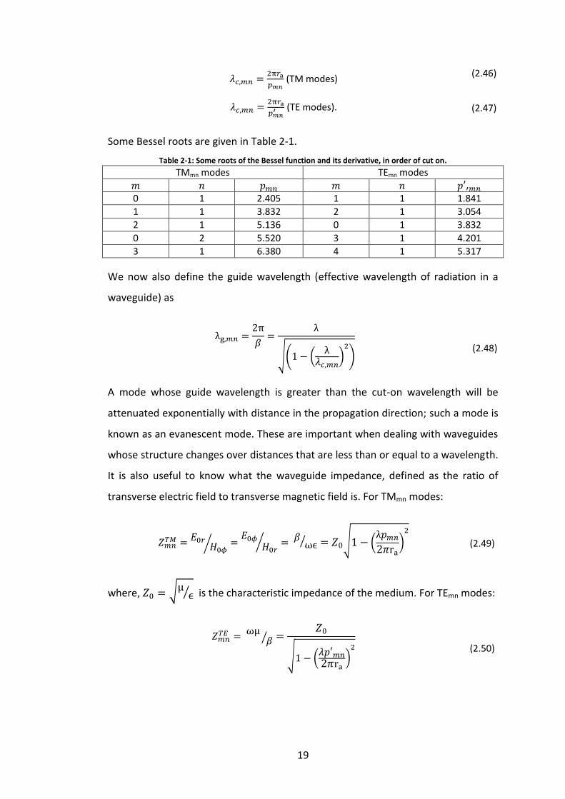
Some Bessel roots are given in Table 2-1.
Table 2-1: Some roots of the Bessel function and its derivative, in order of cut on.
TMmn modes TEmn modes
0 1 2.405 1 1 1.841
1 1 3.832 2 1 3.054
2 1 5.136 0 1 3.832
0 2 5.520 3 1 4.201
3 1 6.380 4 1 5.317
We now also define the guide wavelength (effective wavelength of radiation in a
waveguide) as
(2.48)
A mode whose guide wavelength is greater than the cut-on wavelength will be
attenuated exponentially with distance in the propagation direction; such a mode is
known as an evanescent mode. These are important when dealing with waveguides
whose structure changes over distances that are less than or equal to a wavelength.
It is also useful to know what the waveguide impedance, defined as the ratio of
transverse electric field to transverse magnetic field is. For TMmn modes:
(2.49)
where, is the characteristic impedance of the medium. For TEmn modes:
(2.50)

20
Some plots of the electric field power distribution and direction for a circular
waveguide of arbitrary radius are shown in Figure 2.2
Figure 2.2: Transverse electric field patterns of some circular TE and TM modes showing field power (linear scale) and direction. The arrows are uniform in length and represent the direction of the field only.
In order to generate the plots in Figure 2.2 the and components of the fields
were found using equations (3.11) to (3.18).
2.2 Rectangular waveguides
Fields in hollow metal rectangular waveguides can be found in a similar way to
circular waveguides. By solving the wave equation for the longitudinal and
fields as functions of the transverse components (in this case x and y) and applying
boundary conditions, the transverse fields can be described as functions of the
longitudinal fields (similar to equations (2.22) to (2.25)). Solving this leads to
equations 2.31.1 to 2.31.4. Here the boundary conditions are defined by the guide
dimensions a and b (see Figure 2.3).
TE11 TM11
TE32 TM32

21
The modal equations are given in (19) as:
TM modes:
(2.51)
(2.52)
(2.53)
(2.54)
TE modes:
(2.55)
(2.56)
(2.57)
(2.58)
where,
(2.59)
b x
y
a
z
Figure 2.3: Geometry of a rectangular waveguide (by convention the longer side is always in the x-direction and called ‘a’).

22
As before it is now possible to define a cut-on wavelength from the properties of ,
which must be real for a mode to propagate:
(2.60)
Here and are the mode orders or the number of half wavelengths that fit
across the guide in the x and y directions, respectively. It should be noted that since
magnetic field lines must be a closed loop both and are needed for the TM
modes, making the TM11 mode the lowest order TM mode. Since TE modes have a
non-zero it is possible to have TEm0 modes and indeed TE10 is the fundamental
propagating mode in a rectangular waveguide. Guide wavelength and modal
impedance can be calculated as before (equations (2.48), (2.49) and (2.50)). Some
transverse electric field patterns of a rectangular waveguide are shown in Figure
2.4.
TE10 TM11
TM11 TM23
Figure 2.4: Transverse electric and transverse magnetic field patterns of some rectangular modes showing field power (linear scale) and direction.

23
2.3 Corrugated cylindrical waveguides & horn antennas
2.3.1 Waveguides as antennas
As well as being used as circuit elements to transfer high frequency signals
waveguides have been widely used as antennas in scientific and
telecommunications projects. By flaring out the waveguide to an aperture which is
usually significantly larger than the normal waveguide dimensions, the
guide-wavelength can be made to match the free-space wavelength, meaning there
will be an insignificant amount of reflection at this junction. This allows a signal to
be transmitted or received at specific frequencies. This idea is largely used in
reflector telescopes where the antenna is used as a feed for the detector (Figure
2.5).
These antennas are commonly referred to as feed horns or horn antennas due to
their resemblance to musical horns. The job of an antenna is to produce a beam
which has a desired width, side-lobe level, beam symmetry and cross-polarization
level. Due to the principle of reciprocity the beam produced by the antenna acting
as a radiator is exactly the beam that will couple to the antenna acting as a receiver.
The aperture fields of horn antennas have the same power distribution as the fields
inside a waveguide of the same shape, but with a phase curvature depending on the
flare length of the horn. The far-field can be worked out, if the aperture field is
known, by several methods, including via a Fourier-transform, using the Fresnel
diffraction integral or the Gaussian beam mode approximation. A typical far-field
Primary reflector
Secondary reflector
Feed horn
Figure 2.5: Example of a Cassegrain reflector antenna (left) and a standard smooth-walled conical horn antenna (right).

24
pattern is described by displaying a cut through the 0° and 90° (or E and H) planes
and a 45° cut to show cross-polarization, with power (in dB) as the dependent
variable and off-axis distance as the independent variable, as shown in Figure 2.6.
2.3.2 Hybrid modes
Hybrid modes are formed when both TE and TM modes are propagating in a
waveguide, and are a coherent linear combination of them. Possibly the most
important hybrid mode is the HE11 mode, which will feature heavily in this thesis.
This mode is highly desirable due to its rotational symmetry, high level of on-axis
power (which leads to low side-lobes in the far-field) and suppressed cross-polar
content.
These properties of the HE11 mode depend on the relative power of TE11 and TM11
modes. It is often stated (22) that the ideal HE11 mode has 85% TE11 and 15% TM11
without explaining where these levels come from. However, great insight can be
gained by simply examining the cross-polar content of a HE11 mode while varying
Figure2.6: Far-field beam pattern from a corrugated conical horn antenna designed by the author for the WR-10 band at 91.25GHz.

25
the ratio of TE11 power to TM11 power. This can be done using the functions in
(2.61) and (2.62).
(2.61)
(2.62)
where
is the total power in the -component of the TE11 field (cross-polar
direction), is a constant which is varied from 0.01 to 1 and represents the fraction
of the total power in the TE11 mode. Assuming a perfect HE11 mode means that if
there is a fraction, , of the power in the TE11 mode there must be of the
power in the TM11 mode. (
and are calculated using
equations (3.11) to (3.18)). The denominator in equations (2.61) and (2.62) is the
total power in the mode. is therefore the fraction of cross-polar power and
the fraction of co-polar power. These are plotted, as functions of in Figure
2.7.
Figure 2.7: Plots illustrating the variation in crosspolar(top) and copolar power with ratio of TE11 to TM11

26
Examining Figure 2.7 it is clear that, even in the worst case the crosspolar content of
a HE11 mode (made up of TE11 and TM11 only) is only 25% of the total power,
however by choosing the correct ratio of TE11 to TM11 this can be reduced to
around 1% or less. The top plot of this figure shows that the crosspolar content is
minimized when the ratio of TE11 to TM11 power is in the range 0.85 to 0.90,
conversely the copolar content is maximized in this scenario, clearly demonstrating
that the ideal ratio of TE11 to TM11 power is in this range.
The original idea of using these two modes to produce the desired radiation pattern
in a conical horn was conceived by P. D. Potter in 1963 (23). By using a smooth-
walled conical horn, with initially only the TE11 mode excited in the throat and a
sudden step (as shown in Figure 2.8) he allowed the TM11 to cut on (although the
TE21 mode cuts on before the TM11, no power will couple from a TE11 to a TE21 as
they are of different azimuthal order and are therefore orthogonal). He achieved
the desired beam characteristics of side-lobe suppression and beam symmetry in all
planes (after allowing the two modes to come into phase).
This idea was then refined (24) leading to what is now know as the Pickett-Potter
horn, where, for ease of construction purposes, the slant length of the horn is used
to bring the two modes into phase (Figure 2.9).
Only TE11 can propagate here
TM11 excited here
Length of phasing section chosen to
bring the two modes into phase.
Figure 2.8: Geometry of a Potter horn

27
It is possible to produce an ideal HE11 mode using both of these horns, resulting in
the field pattern shown in Figure 2.10, however they are limited to operation over a
relatively small bandwidth compared to corrugated waveguides/horn antennas.
Figure 2.10: Electric field pattern (power (linear) and direction) for an ideal HE11 mode. Plotted using equation (2.63) (25) with set to 70 mm and set to 3 mm.
The electric field of a HE11 mode is given by:
(2.63)
(2.64)
where is the off-axis distance, is the aperture radius of the horn and is the
slant length of the horn.
Figure 2.9: Pickett-Potter horn. D1 = 1.036λ, D2 = 1.295λ, L = 13.53λ, θ = 15°. θ is known as the flare angle of the horn and is known as the slant length
L
D1
D2
θ

28
2.3.3 Corrugated waveguides
Another, more broadband way to produce a HE11 mode is by adding corrugations to
the inner wall of a circular waveguide (Figure 2.11). These corrugations, when
designed correctly, can have the effect of creating equal boundary conditions for
the electric and magnetic fields of an EM-wave, as will be discussed further in
chapter 3, this leads to generation of a HE11 mode.
To understand how an EM wave propagates inside such a structure is not as simple
as the previously described smooth-walled waveguide; the non-uniform boundary
conditions due to the corrugations make the electric and magnetic field equations
more difficult to derive in a corrugated waveguide. A derivation of the propagation
equation for modes in such a guide is given in the appendix of(22). Various methods
of analysing corrugated cylindrical waveguides will be discussed in chapter 3.
Slot
Ridge
Waveguide axis
r1
r0 t
d
p
w
y
z
x
Figure 2.11: Corrugated waveguide geometry.

29
2.4 Summary
This chapter began with an introduction to the concept of waveguides as carriers of
EM signals at wavelengths which are too small for standard circuitry due to
limitations in the size of the circuits, yet too large to carry useful amounts of power
via free-space propagation, due to diffraction. A detailed derivation of the
properties of EM-fields in circular waveguides was given next, leading to the
formulae for the TE and TM modes and their characteristics such as cut-on
frequency, guide-wavelength and wave-impedance. The TE and TM modes of
rectangular waveguides and their characteristics were described after this.
The use of waveguides as high-gain antennas (horn antennas) was then discussed,
pointing out how the guide-wavelength must be made to match the free-space
wavelength at the horn aperture in order to match the impedance at this point.
Hybrid modes were then introduced as linear combinations of coherent TE and TM
modes with emphasis placed on the HE11 mode, which has the desirable properties
of rotational symmetry, on-axis power and linear-polarization. An analysis of the
optimum ratio of TE11 to TM11 (85:15) for minimum cross-polarization was
performed, resulting in the curves shown in Figure 2.7. The Potter horn and Pickett-
Potter horn were then described as horns capable of generating a HE11 mode over
small bandwidths. A simple equation describing an ideal HE11 mode at the aperture
of a horn was then given along with a 2-dimensional plot of this mode. Finally
corrugated waveguides were introduced as a more broadband way to generate a
HE11 mode. These waveguides are the subject of the next chapter.

30
3. Conical horn analysis methods
In this chapter I will give a description of the various mathematical and
computational techniques that I used for the analysis and design of corrugated horn
antennas. There will first be a discussion of the surface impedance model which
leads to formulation of the hybrid mode field equations and a characteristic
equation for the propagation coefficients of these modes. Following this will be a
description of the mode matching technique which was used most often for
designing the horns due to its computational efficiency and relative simplicity.
Finally the software package Computer Simulation Technology: Microwave Studio
(CST) (26), which uses the finite element technique to model structures interacting
with electromagnetic radiation, will be examined.
3.1 The surface impedance model
The surface impedance model of corrugated waveguides is useful for gaining an
approximate understanding of how corrugations affect the electromagnetic fields
inside the waveguide and for predicting radiation patterns. It works when there are
enough corrugations per wavelength (3 or more is usually enough), so that the
corrugated surface creates an anisotropic-impedance at the waveguide walls, and
when the horn has a constant flare angle, or linear profile. It is also assumed that
only the lowest order TM mode can exist in the slots. The azimuthal component of
the reactance is approximately 0, i.e. the ridges look like a perfectly conducting
surface in the azimuthal-direction, the longitudinal component of the reactance
depends on the depth of the slots and the size of the inner radius, r1 in Figure 2.11.
These boundary conditions lead to solutions for the fields which are independent.
According to (27) the boundary conditions can also be stated as
(3.1)
(3.2)
where,
and d, and are as shown in Figure 2.11.
(3.3)

31
To achieve beam symmetry in both principal planes we would also like at
the waveguide walls. From equations (2.32) and (2.28) we know that for a TE
mode is a function of the component only and for a TM mode is a function of
only. However since the corrugations allow only TM modes to be present at the
walls in a slot is controlled completely by
which at the top of the slots is
proportional to the of a TM mode. This is expressed in (3.4):
Examining equation (3.3) it is clear that when
, making . Now
, and are all zero in the slots. This is known as the open-circuit condition,
as in the theory of transmission lines any circuit element providing infinite
reactance is called an open-circuit. Under this condition the azimuthal components
of the electric and magnetic fields see similar boundary conditions and show a
smooth beam edge-taper leading to desirable axial beam symmetry with low side-
lobes and low cross-polarization. In general it is also assumed that the slot width is
larger than the ridge width ( ) in order to reduce frequency sensitivity,
however as will be discussed in Chapter 4, in the narrow part of the horn this isn’t
always necessarily the best arrangement.
3.1.1 Hybrid mode analysis
Following on from the previous assumptions it is possible to treat a linear
combination of TE and TM modes as a single hybrid mode. The longitudinal
components of both sets of orthogonal mode for the electric and magnetic fields
can be written as in (22).
At
Also, from (3.2)
(3.4)
(3.5)

32
where is known as the normalised hybrid factor and measures the relative
strengths of TE to TM components of the hybrid modes. A hybrid mode is said to be
balanced when , meaning that the conditions leading to have been
met (if is non-zero hybrid modes can propagate and when is infinite we get
balanced hybrid modes). Solving for the transverse field components using these
two values of leads to two sets of modes corresponding to these values. When
we call the modes HEmn and when we call them EHmn. The majority
of the work done for this thesis involved so-called “single-moded” horns where only
one hybrid mode is propagating (namely the HE11 mode), for this reason I will only
describe the transverse fields for the HE1n and EH1n modes as written by (27):
where are the (n = 1, 2, 3…n) roots of and are the (n = 1, 2, 3…n) roots
of . In this case
so now the condition that forces .
Examination of (3.7) shows that this eliminates the cross-polar ( ) component of
the HE field.The characteristic equation for the propagation constant (assuming
no space-harmonics, i.e. only the fundamental TM mode) as given by (22) can be
used to plot dispersion curves for the hybrid modes. This equation is
(3.6)
HE1n modes:
(3.7)
EH1n modes: (3.8)
(3.9)
where
,
33
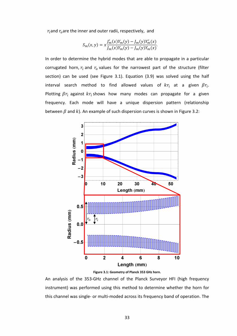
In order to determine the hybrid modes that are able to propagate in a particular
corrugated horn, and values for the narrowest part of the structure (filter
section) can be used (see Figure 3.1). Equation (3.9) was solved using the half
interval search method to find allowed values of at a given
Plotting against shows how many modes can propagate for a given
frequency. Each mode will have a unique dispersion pattern (relationship
between and ). An example of such dispersion curves is shown in Figure 3.2:
An analysis of the 353-GHz channel of the Planck Surveyor HFI (high frequency
instrument) was performed using this method to determine whether the horn for
this channel was single- or multi-moded across its frequency band of operation. The
and are the inner and outer radii, respectively, and
Figure 3.1: Geometry of Planck 353 GHz horn.

34
term multi-moded means more than one hybrid mode is propagating. Multi-mode
antennas can produce an antenna reception pattern close to a top-hat function and
are desirable in many applications due to their high sensitivity/ higher power
throughput.
Figure 3.2: Dispersion curves for the Planck 353 GHz channel is the azimuthal order of a mode. Dashed orange lines show the edges of the band. (This plot was done in conjunction with Stephen Scully of
Maynooth University).
Figure 3.2 shows the results for the 353 GHz channel of the ESA Planck Surveyor,
which was a mission to measure the cosmic microwave background radiation.
According to the hybrid mode model a varying number of modes will propagate at
different frequencies in the band, a total of 10 modes can propagate, with the
maximum number of 7 propagating modes occurring at approximately 460 GHz. The
hybrid mode model is quick and very useful for the initial stages of horn design and
verification. In order to fully account for more complex horn profiles, however,
other more detailed methods should be used. These are described next.
One interesting thing to note from these dispersion diagrams is that unlike smooth-
walled horns (see e.g. (2.59)), corrugated horns have a high frequency cut off as
well a low frequency cut off, which makes them better filters than smooth-walled
horns.
0 100 200 300 400 500 600
0
1
2
3
4
5
6
7
8
9
10
0 1 2 3 4 5 6 7 8 9 10
v [GHz]
ßr i
kri
m = 0
m = 1
m = 2
35
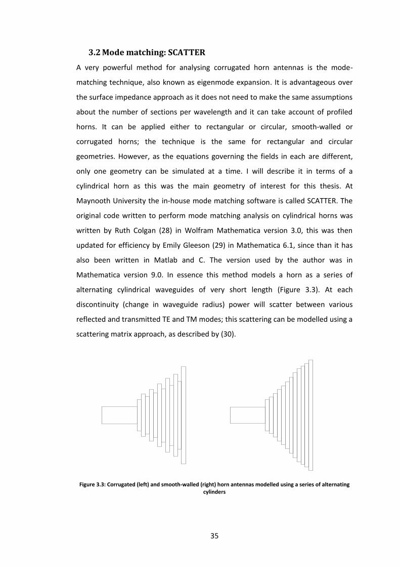
3.2 Mode matching: SCATTER
A very powerful method for analysing corrugated horn antennas is the mode-
matching technique, also known as eigenmode expansion. It is advantageous over
the surface impedance approach as it does not need to make the same assumptions
about the number of sections per wavelength and it can take account of profiled
horns. It can be applied either to rectangular or circular, smooth-walled or
corrugated horns; the technique is the same for rectangular and circular
geometries. However, as the equations governing the fields in each are different,
only one geometry can be simulated at a time. I will describe it in terms of a
cylindrical horn as this was the main geometry of interest for this thesis. At
Maynooth University the in-house mode matching software is called SCATTER. The
original code written to perform mode matching analysis on cylindrical horns was
written by Ruth Colgan (28) in Wolfram Mathematica version 3.0, this was then
updated for efficiency by Emily Gleeson (29) in Mathematica 6.1, since than it has
also been written in Matlab and C. The version used by the author was in
Mathematica version 9.0. In essence this method models a horn as a series of
alternating cylindrical waveguides of very short length (Figure 3.3). At each
discontinuity (change in waveguide radius) power will scatter between various
reflected and transmitted TE and TM modes; this scattering can be modelled using a
scattering matrix approach, as described by (30).
Figure 3.3: Corrugated (left) and smooth-walled (right) horn antennas modelled using a series of alternating cylinders

36
3.2.1 Mode normalisation and conversion to Cartesian coordinates
The principle of mode matching requires that the total complex power at a
scattering junction is conserved; this requirement can be used to find exact
solutions to the transverse modal field equations. By setting
, where
is the Poynting vector and gives the magnitude and
direction of energy flow at any point in the waveguide, the complex power is
normalised to unity over a cross-section of the waveguide.
Since cross-polarization is something antenna designers are very interested in it
makes sense to write the modal equations in terms of Cartesian coordinates as
opposed to cylindrical polar coordinates which have been used until now. Using the
transformation relations given in (3.10) and the above normalisation condition the
Cartesian components of the transverse modal fields (given in (2.38) to (2.45)) used
for mode matching are given in (3.11) to (3.18), see e.g. (29).
TEnl modes
(3.10)
(3.11)
(3.12)
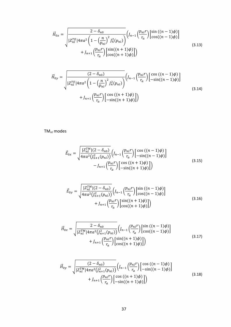
37
TMnl modes
(3.13)
(3.14)
(3.15)
(3.16)
(3.17)
(3.18)

38
is a Kronecker delta function (3.19):
3.2.2 Scattering matrix formalisation
At the transition between each cylindrical section of the waveguide, power
scattering between modes will take place due to the sudden change in
guide-wavelength. This process can be described by a scattering matrix, as will now
be shown.
A set of column matrices and contain the transmission and reflection
coefficients for the fields coming into a section, similarly and contain the
transmission and reflection coefficients for the fields coming out of a section (see
Figure 3.4).
In Figure 3.4 is called the scattering matrix; each junction has a unique
scattering matrix and these matrices can be cascaded to form a single scattering
matrix for the whole horn, which can be used to determine its radiation
characteristics. The forward and reflected scattering matrices are related in the
following way
For a two port system can be written as
(3.19)
. (3.20)
Figure 3.4: Diagram illustrating the relationship between forward and backwards propagating matrices
Port 1 Port 2

39
The elements of are square matrices containing the power coupling coefficients
between all modes at the input with all modes at the output.
Consider the junction in Figure 3.5, for cylindrically symmetric geometries such as
this it turns out that we can consider different azimuthal orders independently, as
modes of different azimuthal order are orthogonal, meaning no power will couple
between them. The scattering matrix for the first azimuthal order can then be
expressed as shown in (3.22)
(3.22)
where refers to the scattering of power from port 2 to port 1, etc.
(3.21)
Figure 3.5: Example of a typical waveguide junction
A B
40
Each column contains the coupling from a given mode of a particular azimuthal and
radial order to every other mode of the same azimuthal order.
The nature of the waveguide mode model means that there could be an infinite
number of possible modes to consider in each section (including evanescent
modes), clearly this is computationally impossible so the number of modes to be
considered is chosen such that a specified amount of the total scattered power is
recovered upon addition of the coupling coefficients. Typically for the examples in
this thesis 30 modes (1 azimuthal order) were sufficient. Combining (3.20) and
(3.21) gives (3.24)
At the input of the horn (usually chosen to be the smaller aperture) it is assumed
that there is no power flowing from the inside of the horn, so is set to zero. For
scattering inside the horn will clearly not be zero. When considering the final
scattering matrix the reflection and transmission coefficients are given by
and The form of the input matrix will vary depending
on the excitation to be simulated. Only single moded operation was considered in
this work, meaning that the first value in was 1 and all others were 0. In this
case the reflection and transmission coefficients are completely characterised by
the and matrices, respectively.
This approach is useful as scattering matrices produced at consecutive junctions in
the horn can easily be cascaded together in the following way (30). Consider two
such matrices:
(3.24)
⇒
(3.23)

41
The cascaded matrix elements are given by:
(3.25)
There are essentially two types of section scattering matrix that need to be
considered: ‘scattering’ along a uniform section and scattering at a discontinuity.
3.2.3 Mode scattering along a uniform section of waveguide
For a uniform section of waveguide power will not scatter between modes,
however the power in a particular mode can change depending on whether it has
cut on or not. Here it is important to consider a large number of evanescent modes
since if the length of the section is very short evanescent modes can still have
significant amplitude at the end of the section. The scattering matrix elements are
given in (30) as:
where is a diagonal matrix ( is the number of TE and TM modes)
whose diagonal elements are calculated by:
where is the propagation constant for the th mode being considered and is
purely real for propagating modes and purely imaginary for evanescent modes. is
the length of the section.
3.2.4 Mode scattering at a waveguide discontinuity
Any sudden change in the geometry of a waveguide (e.g. Figure 3.6) causes a
change in guide wavelength which results in reflections and power scattering
(3.26)
(3.27)
(3.28)

42
between modes. To calculate this power scattering we need to consider the electric
and magnetic fields on either side of the junction (Figure 3.6). These are given by
(30) as:
where the subscripts and indicate the field is on the left or right side of a
junction, respectively, is the number of modes being considered
and and
are the transverse fields of the mode, positive
indicates propagation in the negative direction and negative indicates
propagation in the positive z direction. (We take for the moment the left hand side
(LHS) as the narrower of the two sections).
Recognizing that the fields must be equal at the interface and setting to be zero at
this position leads to the equations (3.33) and (3.34)
(3.29)
(3.30)
(3.31)
(3.32)
Figure 3.6: Waveguide discontinuity. represents a cross sectional area on the LHS of the junction and an area on the RHS.
43
Taking the electric field on the right side of the junction to be zero outside of the
common area ( in Figure 3.6) and considering also the parallel metallic walls
and the orthoganality relationship between modes on the same side of the junction
leads to the simultaneous matrix equations in (3.35) and (3.36):
The elements of [ ] (which is an square matrix) represent the power
coupling between modes on either side of the junction and are calculated using
equation (3.37)
The matrix is an diagonal matrix whose diagonal elements are the self
coupling between mode on the right hand side o f the junction, these elements are
given by equation (3.38)
Similarly the matrix is a diagonal matrix whose diagonal elements are given by
equation (3.39) and represent the self coupling between mode on the left hand side
of the junction.
From equations (3.35) and (3.36) we can write down what the scattering matrix
elements are in terms of and :
(3.33)
(3.34)
(3.35)
(3.36)
(3.37)
(3.38)
(3.39)

44
(3.40)
(3.41)
(3.42)
(3.43)
Due to the different forms of TE and TM modes, will be different when
considering coupling between TE/TE, TE/TM, TM/TE and TM/TM. This is not a
problem for or as there is no scattering between modes upon reflection
since the waveguide radius is constant for incident and reflected modes. Analytical
solutions to these integrals are used in SCATTER to increase computational
efficiency; these solutions are given in Chapter 3 of (29). It should be noted that
these solutions are for propagation from a smaller to larger radius section of
waveguide, going from larger to smaller radius (as is the case for every second
junction in a corrugated horn) will result in a different scattering matrix, Figure 3.7.
However we can consider the case where a > b equivalent to the case when b > a
with the radiation propagating in the opposite direction.
3.2.5 SCATTER algorithm.
In this section the main algorithm used by SCATTER will be discussed. The first step
in running SCATTER is define a horn’s geometry. This is done by creating a list of the
a b a b
Figure 3.7: Two kinds of junction

45
radii and lengths of each cylindrical section. The standard input format adopted is
shown in Table 3-1.
Table 3-1: SCATTER Geometry file input format
Line Column 1 Column 2
1 Operating frequency in GHz
2 Maximum azimuthal order
3 Number of sections (N)
4 N + 3 Length of section
N + 4 2N + 3 Radius of section Number of modes considered for
this section
Using this table SCATTER can cascade the scattering matrices from one section to
the next in the correct order. The number of modes being considered, modenum in
the SCATTER code, is split evenly between TE and TM modes with the TE modes
making up the first half of the scattering matrix (as in (3.22)).
In order to produce a horn’s beam patterns the radiation is considered to be moving
from the small aperture to the large aperture. The main SCATTER algorithm can be
described in the following steps (‘a’ and ‘b’ here will refer to the radius on the left
and right side of a junction, respectively):

46
1. Load in a geometry file. (define total number of section and frequency)
2. This defines the initial radius ‘ao’ and length ‘LLinit’.
3. Populate a diagonal matrix ‘VVinit’ based on equation (3.28).This
represents the scattering along the initial uniform section of the horn.
4. Define initial scattering parameters,
as in
equations (3.26) and (3.27).
5. Set = , set = radius corresponding to ( + 1)th section, set
= length corresponding to ( + 1)th section.
6. If{ , = , = } else If{ , =
= }.(Determines left and right sections, bigger is always on the
left).
7. Calculate and for the junction.
8. Calculate the new for the right-hand section.
9. Calculate using equations (3.40) to (3.43) to
get
10. Combine this with to get (represents propagation of field
through the current section).
11. Cascade with using equations (3.25) to find .
12. Set .
13. Increment ‘index’.
14. If{‘index’ < ‘sections-1’; return to step 7} else{exit loop}.
3.2.6 Radiation patterns
Once the preceding algorithm has been completed for all sections of the horn and
all azimuthal orders, the modal content at the aperture is known and the aperture
field can be calculated using (3.44):
(3.44)
where, is the number of azimuthal orders, is the number of TE and TM modes and
and specify the row and column of the matrix.
For
each
azi
mu
thal
ord
er
For
ind
ex
s
ecti
on
s

47
The majority of corrugated horn antennas are in what is called single mode
operation meaning that only the fundamental HE11 hybrid mode will be propagating
(this mode can be made up of any number of waveguide section TE and TM modes
so long as they are propagating coherently). However at frequencies well above the
cut on for the fundamental mode more than one hybrid mode can propagate, as
was the case in Figure 3.2 for the Planck 353–GHz horn. Carrying out a singular
value decomposition (SVD) of the full scattering matrix to determine its non-zero
singular values allows the number of true independent orthogonal fields (i.e. the
hybrid HE and EH modes) to be found (see e.g.(31)) The rest of this thesis deals
with single mode horns however.
3.3 Finite Integration Technique, CST: Microwave Studio
CST Microwave Studio is a commercially available electromagnetic simulation
package based on the finite integration technique (FIT). It is a very powerful,
complex package with many capabilities. The only facet of CST used for this work
was the antenna simulation tool.
The numerical approach to calculating electric and magnetic field values requires a
spatial-discretisation of the element being modelled in order to define a finite
calculation domain. In CST this is done by dividing the structure into a series of
discrete volume elements called "mesh cells". These can be hexahedral or
tetrahedral depending on the solver type. Maxwell's grid equations (32) are then
used to calculate the electric voltages and corresponding magnetic fluxes along the
edges and through the faces of these shapes, respectively (Figure 3.8). There is also
an orthogonal set of mesh cells where the magnetic voltage and electric fluxes are
calculated. Consider the integral form of Faraday’s law (3.45):
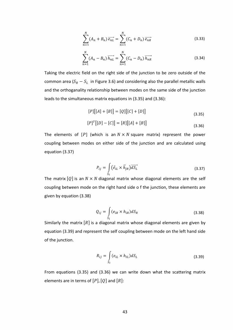
For a mesh cell the closed integral can be rewritten as the sum of four “grid
voltages” ( ), see Figure 3.8. The magnetic flux on the cell face ( )
is equal to , leading to (3.46)
(3.45)
48
Figure 3.8: CST mesh system. Source: CST documentation centre.
Repeating this for all of the cell faces leads to a matrix formulation as shown in
equation (3.47).
Applying a similar scheme to Ampère’s law and Gauss’s divergence laws leads to a
full set of discretised Maxwell’s equations.
3.3.1 Solver Types
CST includes three methods of simulation, or solvers. These are the transient,
frequency domain and eigenmode solvers. Transient is a time domain solver, which
makes it useful for wideband simulations as the effect of a structure on multiple
frequencies can be simulated in a single calculation. Both the transient and
frequency domain solvers make use of the Maxwell’s grid equations as discussed
above, however the transient solver was the only one used in this work.
3.3.2 Setting up a simulation
When setting up a simulation in CST the first step is to create a 3D representation of
the structure you wish to model. The CST user interface (UI) allows for the creation
of several standard 3D shapes (e.g. brick, sphere cone) and implements
(3.46)
(3.47)

49
Constructive Solid Geometry for the Boolean addition of shapes, in this way
arbitrary shapes can be created. This is done in the modelling tab of the UI.
There are several options for material type, which effectively change the value of
and where the mesh intersects the material of the structure being modelled.
However for this work the material was assumed to be a perfect electrical
conductor (PEC), which has the properties and . It is also
possible to create an element of vacuum (free-space) which can be Boolean
subtracted from another element to create, for example, a hollow brick (Figure 3.9).
Figure 3.9: Creating a hollow brick in CST
Once the structure has been built in the 3D modeller, a frequency range must be
defined before the simulation begins. There are several methods for exciting the
structure with an electromagnetic signal. These include plane-wave excitation and
excitation at a waveguide port. The waveguide port method works by generating a
field comprised of the modes in an infinitely long, lossless waveguide of equivalent
geometry at a defined port. Taking the example of the brick in Figure 3.9, two edges
of the entrance to the hollow part of the brick are selected, to define the shape of
the port. CST allows the properties of the port, such as the number of considered
modes, to be chosen and an excitation field will then be generated at this point. A
waveguide port is indicated by a 2D plane coloured red, as seen in Figure 3.10.
PEC brick with vacuum brick
to be subtracted
PEC brick Hollow PEC brick PEC brick

50
The accuracy of a simulation can be greatly affected by the number of sample
points, too few and the results will be inaccurate, however choosing too many will
increase the run time of the simulation unnecessarily. The number of sample points
in CST is the number of mesh-cells being used to represent the structure. This can
be altered by the user (the number of lines per wavelength will define the
dimensions of the mesh-cells with respect to the highest frequency considered). For
structures with very small parts, such as a corrugated horn where the slots and
ridges can be less a tenth of a wavelength, it is important to consider many lines per
wavelength, typically 20 – 30. If the accuracy of a simulation is in doubt CST
provides an adaptive meshing option whereby the size of the mesh is changed
locally by performing multiple runs and reducing the mesh-size until a steady-state,
to certain accuracy, is reached. The waveguide port method also naturally allows for
S-Parameter calculation, as more than one port can be created.
In order to reduce calculation time it is possible to take advantage of symmetries in
a system. Each exploited symmetry reduces the memory requirements by a factor
of 2, leading to a reduced computation time. One practical example is a conical horn
fed by a rectangular waveguide. This is rotationally symmetric about 180°. We can
therefore define two symmetry planes, namely the -plane and the -plane (see
Figure 3.11).
Figure 3.10: Waveguide port shown in red.

51
Figure 3.11: Conical horn with rectangular waveguide feed. Symmetry planes shown in red and green
There are two types of symmetry plane: electric boundary and magnetic boundary.
Electric fields tangential to, and magnetic fields normal to, an electric boundary
symmetry plane go to zero at the plane and are symmetric about the plane. The
converse is true for magnetic symmetry. In the case of Figure 3.12, the field in the
rectangular WG is -polarized so we set the -plane to have an electric boundary
and the -plane to have a magnetic boundary. This feature can be accessed in the
simulation tab by pressing the boundaries button and in the pop-up menu selecting
symmetry planes. An example of setting this up is shown in Figure 3.12).
Figure 3.12: Setting up symmetry planes in CST
-plane
-plane
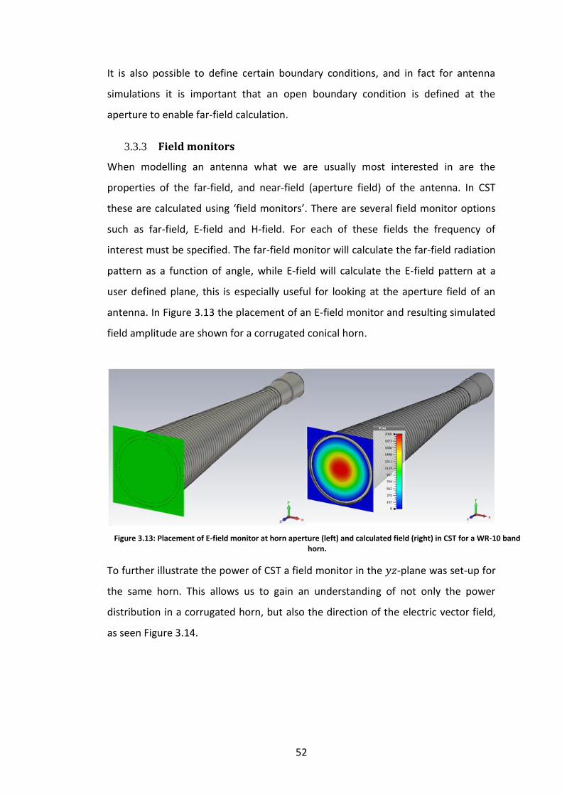
52
It is also possible to define certain boundary conditions, and in fact for antenna
simulations it is important that an open boundary condition is defined at the
aperture to enable far-field calculation.
3.3.3 Field monitors
When modelling an antenna what we are usually most interested in are the
properties of the far-field, and near-field (aperture field) of the antenna. In CST
these are calculated using ‘field monitors’. There are several field monitor options
such as far-field, E-field and H-field. For each of these fields the frequency of
interest must be specified. The far-field monitor will calculate the far-field radiation
pattern as a function of angle, while E-field will calculate the E-field pattern at a
user defined plane, this is especially useful for looking at the aperture field of an
antenna. In Figure 3.13 the placement of an E-field monitor and resulting simulated
field amplitude are shown for a corrugated conical horn.
To further illustrate the power of CST a field monitor in the -plane was set-up for
the same horn. This allows us to gain an understanding of not only the power
distribution in a corrugated horn, but also the direction of the electric vector field,
as seen Figure 3.14.
Figure 3.13: Placement of E-field monitor at horn aperture (left) and calculated field (right) in CST for a WR-10 band horn.

53
Figure 3.14: Power distribution in the yz-plane (x = 0) (top) and direction of the electric field lines in a corrugated horn (bottom).
3.4 Comparison of SCATTER and CST
Clearly, SCATTER and CST are very different methods of simulation and this is
extremely useful for cross-verification of results. SCATTER and CST have been
shown to give good agreement in situations where both techniques are applicable,
for examples of far-field comparisons see, for example, (33). There is also a
comparison of the near-fields calculated for a corrugated conical horn shown in
Figure 3.15. The advantages and disadvantages of the two software packages are
listed in Table 3-2.
Table 3-2: Comparison of SCATTER and CST
SCATTER CST
Fast Slow
Computationally easy Computationally intensive
Symmetric systems only (current version) Allows for any shape
One type of geometry (rectangular or circular) All geometries
In-house Commercial (“black box”)
In summary, for symmetric systems employing only one geometry SCATTER is the
preferred choice due to its computational speed. However more complicated
asymmetric systems with multiple shapes can be catered for by CST as FIT is a much
more general simulation technique.

54
One of the main advantages of SCATTER is that it is in-house which mean we have
access to the code itself and so can have complete control over a simulation and
can customise automation and optimization. I have made use of both simulation
techniques for the work in this thesis.
Figure 3.15: SCATTER vs. CST aperture fields for a WR 1.0 horn. (The small discrepancies are likely due to the fact that SCATTER does not account for the step to free-space at the aperture but CST does).
55
3.5 Summary
In this chapter I have introduced three methods of analysis for corrugated horn
antennas. I began by describing the surface impedance model, which treats the
corrugation like a uniform surface impedance at the inner walls of a corrugated
waveguide or horn antenna. This model allows us to derive a mathematical
description for the behaviour of an electric field inside such a corrugated waveguide
and provides an explanation as to why choosing quarter-wavelength deep
corrugations lead to a desirable on-axis, rotationally symmetric, linearly polarized
beam (HE11 mode). Using this model it is also possible to calculated the hybrid (HE
or EH) mode modal dispersion curves at a given section of a corrugated horn (i.e.
specific values of the inner and outer radii ( and )). This is an approximate but
useful way of determining the number of possible propagating hybrid modes at the
narrowest part of a corrugated horn which behaves as a bandpass-filter. An
example of this technique was given for the Planck surveyor 353-GHz channel horn
antenna.
The second method that was described was the mode-matching technique,
specifically in relation to Maynooth University’s in-house code, SCATTER. The
mode-matching technique is extremely useful for simulating the antenna properties
(reflection, transmission and radiation patterns) of corrugated horns. Each section
of the horn, i.e. each corrugation, is treated like a waveguide supporting TE and TM
modes, these modes will be either reflected or transmitted at the interface
between two sections. Power will also be scattered between the modes for the
transmitted field. These effects can be modelled using a two-port scattering matrix
approach. The method used by SCATTER for these simulations was outlined in detail
and the method of calculating the radiation pattern was given. There was also a
brief discussion on simulating a multimode horn using SCATTER using singular value
decomposition.
The final simulation approach was the finite integration technique. This is the
method used by CST: Microwave Studio, a commercially available electromagnetic
simulation software package. There was a description of this technique, as it is
employed by CST, followed by an outline of how to set up a simulation. Some of the

56
capabilities of CST were also discussed, including the usefulness of field monitors.
Finally there was a comparison of CST and SCATTER along with their advantages and
disadvantages for different situations.

57
4. Designing corrugated conical horn antennas
In this section I describe much of the work I have done in the design and analysis of
corrugated horn antennas, which are used to couple EM radiation from a
rectangular waveguide to either free-space or to a large diameter corrugated
cylindrical waveguide. There are three main design steps involved, at each step the
goal is to couple radiation between two regions with different propagation
properties: (1) the transition from rectangular to circular waveguide (2) the
transition from circular waveguide to the corrugated horn throat and (3) the
transition from throat to aperture (this is the main body of the horn), at this point in
the system there will be a transition to either free-space or to a corrugated circular
waveguide.
4.1 System design requirements
As discussed in Chapter 1, SWISSto12 would like to manufacture a series of
corrugated horn antennas to function as free-space radiators or to be used in
conjunction with their material characterisation kits (MCKs). Each horn is to be
designed to work across one of the industry standard WR waveguide bands. Table
4-1 describes the properties of the WR bands and corresponding rectangular
smooth-walled waveguides which will be referred to as “WR guides”.
Table 4-1: WR waveguide bands, frequencies and dimensions. Source: Virginia Diodes (virginiadiodes.com)

58
The horns designed in this thesis will be used as part of a vector network analyser
(VNA) laboratory measurement system. Measurements at GHz and THz frequencies
are often made using VNAs which can measure both the amplitude and phase of an
EM wave. VNAs use a port system similar to SCATTER and CST and the
measurements are described in terms of S-parameters in exactly the same way.
The VNA itself can generate an oscillating signal (state of the art VNAs can reach up
to 40 GHz), however to reach the frequencies of interest a frequency multiplier
(frequency extension module) is used to step up the frequency into the correct
band. These mixers are designed to operate across the WR frequency bands and
output their signal through a rectangular WR waveguide. A fuller description of VNA
and frequency extension module operation will be given in chapter 5.
The the VNA frequency extension modules output their signal via rectangular WR
guides and therefore the corrugated horns must be connected to these. This is a
common transition for many millimetre-wave systems and is usually achieved by
connecting the corrugated horn throat to the rectangular WG through a piece of
smooth-walled circular WG, as seen in Figure 4.1.
Figure 4.1: Waveguide network to be designed. The dashed cylinder represents the optional corrugated wave, which would be used as part of the material characterisation kit.
To VNA
Rectangular WR guide
Smooth-walled circular guide
Corrugated conical horn antenna
Corrugated waveguide
To be designed
To sample to be measured

59
From this we can define three design stages as follows:
1. Transition from rectangular to circular smooth walled WG.
2. Transition from circular smooth walled WG to corrugated horn.
3. Transition from small diameter “throat” of horn to larger aperture.
4.1.1 Design goals
The design goals for these horns are shown in Table 4-2:
Table 4-2: Design goals for SWISSto12 horns.
Parameter Goal
Peak S11 dB across the band
Peak cross-polar power dB across the band
HE11 modal purity > 92 % across the band
In some cases only the S11 and HE11 were examined in detail as performance
metrics, this is justified as the HE11 is a linearly polarized field and strong coupling to
it implies low levels of cross-polarization. There were also some mechanical
limitations that needed to be taken into account, such as the manufacturing
precision and keeping the horn as short as possible to reduce the building cost. The
aperture size was also pre-determined by SWISSto12®, but this was flexible in some
cases.
4.2 Rectangular to circular transition
The most critical factor when designing a rectangular to circular transition is the
reflection at the junction, which we want to minimize. In electrical engineering the
reflection coefficient on a transmission line is written in the following way:
where is the load impedance and is the source impedance.
The reflection coefficient will be minimized when the source and load impedance
are equal, they are then said to be ‘matched’. The waveguide impedance
expressions in (2.49) and (2.50) can be generalized for any shape waveguide to the
equations in (4.2):
(4.1)
(4.2)
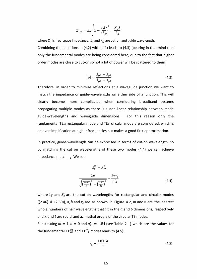
60
Combining the equations in (4.2) with (4.1) leads to (4.3) (bearing in that mind that
only the fundamental modes are being considered here, due to the fact that higher
order modes are close to cut-on so not a lot of power will be scattered to them):
Therefore, in order to minimize reflections at a waveguide junction we want to
match the impedance or guide-wavelengths on either side of a junction. This will
clearly become more complicated when considering broadband systems
propagating multiple modes as there is a non-linear relationship between mode
guide-wavelengths and waveguide dimensions. For this reason only the
fundamental TE01 rectangular mode and TE11 circular mode are considered, which is
an oversimplification at higher frequencies but makes a good first approximation.
In practice, guide-wavelength can be expressed in terms of cut-on wavelength, so
by matching the cut on wavelengths of these two modes (4.4) we can achieve
impedance matching. We set
where and
are the cut-on wavelengths for rectangular and circular modes
((2.46) & (2.60)), and are as shown in Figure 4.2, and are the nearest
whole numbers of half wavelengths that fit in the and dimensions, respectively
and and are radial and azimuthal orders of the circular TE modes.
Substituting and (see Table 2-1) which are the values for
the fundamental and
modes leads to (4.5).
where is free-space impedance, and are cut-on and guide wavelength.
(4.3)
(4.4)
(4.5)
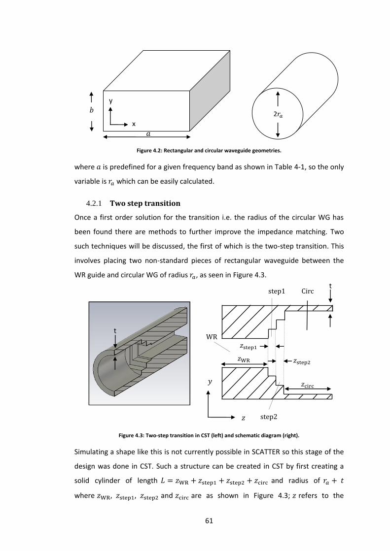
61
Figure 4.2: Rectangular and circular waveguide geometries.
where is predefined for a given frequency band as shown in Table 4-1, so the only
variable is which can be easily calculated.
4.2.1 Two step transition
Once a first order solution for the transition i.e. the radius of the circular WG has
been found there are methods to further improve the impedance matching. Two
such techniques will be discussed, the first of which is the two-step transition. This
involves placing two non-standard pieces of rectangular waveguide between the
WR guide and circular WG of radius , as seen in Figure 4.3.
Figure 4.3: Two-step transition in CST (left) and schematic diagram (right).
Simulating a shape like this is not currently possible in SCATTER so this stage of the
design was done in CST. Such a structure can be created in CST by first creating a
solid cylinder of length and radius of
where and are as shown in Figure 4.3; refers to the
t
x
y
2
t

62
dimension of the component and is the thickness of the waveguide walls. This
must be greater than the skin depth of the material being used. We are using a
perfect electrical conductor (PEC) for the simulation and the skin depth of a PEC is
0 m, however the real components will stainless steel coated in gold, which has a
skin depth on the order of nm at THz frequencies, so is usually, somewhat
arbitrarily, set to be approximately one fifth of a wavelength. Following the method
outlined in chapter 3 it is possible to subtract the appropriate shapes from this
cylinder. By defining the dimensions of the shapes as variables, in the way shown in
Figure 4.4 for example, it is possible in CST to perform a parameter sweep analysis
or to implement an optimization for the transition.
Figure 4.4: Defining a brick using variables in CST, with the centre of the brick on the axis of CST’s coordinate system.
The longitudinal dimensions of and were initially chosen to be about a
quarter of a guide wavelength at the central frequency of the band. This will have
the same effect as the quarter-wavelength films used for anti-reflective coatings.
Radiation reflected at the junction between and will be coherent and
radians out of phase with radiation reflected at the junction,
producing destructive interference between the reflected waves at this point. The
transverse dimensions are chosen initially so the steps between the WR guide and
the circular guide are all equal by using the relationships shown in (4.6).
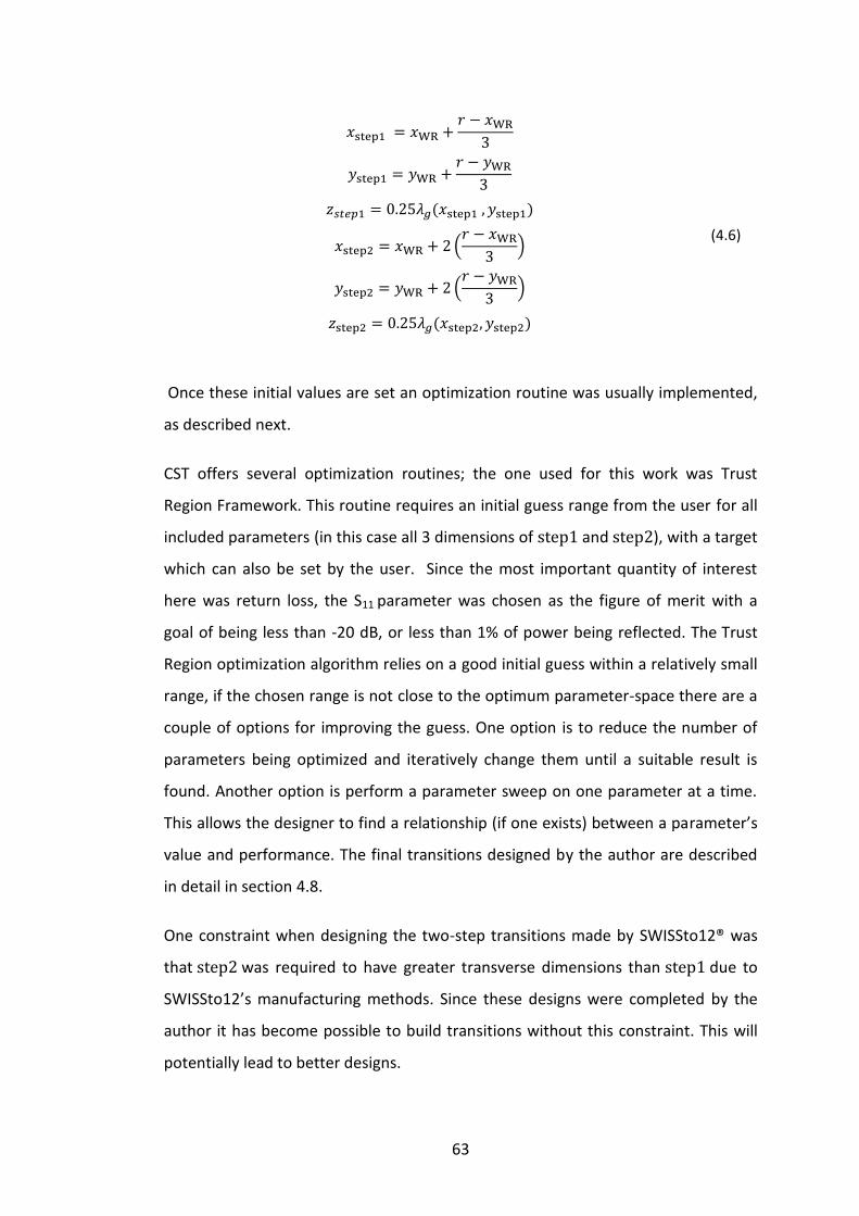
63
Once these initial values are set an optimization routine was usually implemented,
as described next.
CST offers several optimization routines; the one used for this work was Trust
Region Framework. This routine requires an initial guess range from the user for all
included parameters (in this case all 3 dimensions of and ), with a target
which can also be set by the user. Since the most important quantity of interest
here was return loss, the S11 parameter was chosen as the figure of merit with a
goal of being less than -20 dB, or less than 1% of power being reflected. The Trust
Region optimization algorithm relies on a good initial guess within a relatively small
range, if the chosen range is not close to the optimum parameter-space there are a
couple of options for improving the guess. One option is to reduce the number of
parameters being optimized and iteratively change them until a suitable result is
found. Another option is perform a parameter sweep on one parameter at a time.
This allows the designer to find a relationship (if one exists) between a parameter’s
value and performance. The final transitions designed by the author are described
in detail in section 4.8.
One constraint when designing the two-step transitions made by SWISSto12® was
that was required to have greater transverse dimensions than due to
SWISSto12’s manufacturing methods. Since these designs were completed by the
author it has become possible to build transitions without this constraint. This will
potentially lead to better designs.
(4.6)
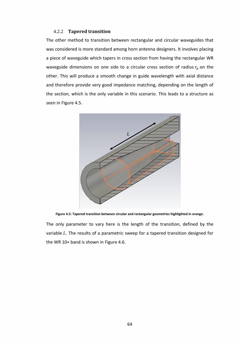
64
4.2.2 Tapered transition
The other method to transition between rectangular and circular waveguides that
was considered is more standard among horn antenna designers. It involves placing
a piece of waveguide which tapers in cross section from having the rectangular WR
waveguide dimensions on one side to a circular cross section of radius on the
other. This will produce a smooth change in guide wavelength with axial distance
and therefore provide very good impedance matching, depending on the length of
the section, which is the only variable in this scenario. This leads to a structure as
seen in Figure 4.5.
Figure 4.5: Tapered transition between circular and rectangular geometries highlighted in orange.
The only parameter to vary here is the length of the transition, defined by the
variable . The results of a parametric sweep for a tapered transition designed for
the WR 10+ band is shown in Figure 4.6.
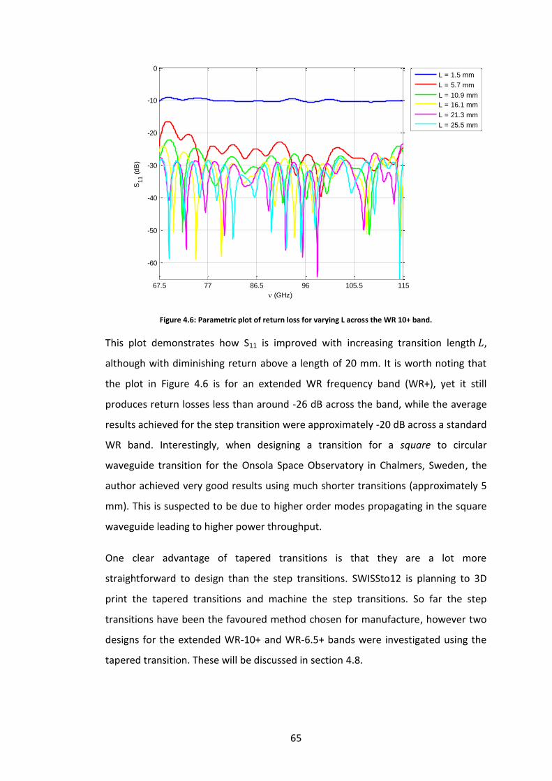
65
Figure 4.6: Parametric plot of return loss for varying L across the WR 10+ band.
This plot demonstrates how S11 is improved with increasing transition length ,
although with diminishing return above a length of 20 mm. It is worth noting that
the plot in Figure 4.6 is for an extended WR frequency band (WR+), yet it still
produces return losses less than around -26 dB across the band, while the average
results achieved for the step transition were approximately -20 dB across a standard
WR band. Interestingly, when designing a transition for a square to circular
waveguide transition for the Onsola Space Observatory in Chalmers, Sweden, the
author achieved very good results using much shorter transitions (approximately 5
mm). This is suspected to be due to higher order modes propagating in the square
waveguide leading to higher power throughput.
One clear advantage of tapered transitions is that they are a lot more
straightforward to design than the step transitions. SWISSto12 is planning to 3D
print the tapered transitions and machine the step transitions. So far the step
transitions have been the favoured method chosen for manufacture, however two
designs for the extended WR-10+ and WR-6.5+ bands were investigated using the
tapered transition. These will be discussed in section 4.8.
67.5 77 86.5 96 105.5 115
-60
-50
-40
-30
-20
-10
0
(GHz)
S11 (
dB
)
S11
vs frequency for various transition lengths
L = 1.5 mm
L = 5.7 mm
L = 10.9 mm
L = 16.1 mm
L = 21.3 mm
L = 25.5 mm

66
4.3 Circular waveguide to corrugated horn transition
Once a suitable radius ( ) for the smooth-walled circular waveguide has been
found using (4.5) it is possible to begin designing the transition to a corrugated horn
throat. The goal here is not only to match the impedance between the smooth
walled and corrugated sections but to launch the balanced HE11 mode in the horn.
For this reason the throat of the horn is sometimes referred to as the mode
convertor or mode launching section (34). Again, two design strategies were
examined, the first of which was outlined in (22) and will be referred to as the
‘Claricoats throat’. The second was described in (27) and will be referred to as the
‘Zhang throat’.
The first step in this design, which is the same for both throat types, is to include at
least one half of a wavelength of smooth-walled cylindrical waveguide before
stepping into the corrugated section. This is to ensure that any evanescent modes
which may be propagating are at sufficiently low amplitude at the junction to the
corrugated section that they won’t couple to higher order modes or contribute
detrimental amounts of power to the return loss.
4.3.1 Claricoats throat
The two main issues with this transition are reflections caused by a sudden change
in guide wavelength, but also the excitation of undesirable modes in the corrugated
section. The HE11 and EH11 modes have very close cut-on points so it is easy to excite
the EH11 mode when trying to attain the HE11. The EH11 has relatively high cross-
polarization and is a “surface-wave” which means most of the power is at the edge
of the waveguide walls, the opposite of what is desired for these horns. We can
overcome the problem of high levels of reflection by considering the boundary
conditions in both types of waveguide, which determine the properties of the
waveguide modes. In an ideal smooth walled waveguide the surface reactance
and in a corrugated waveguide
as seen in
equation
(3.3). Examining the corrugated waveguide surface reactance equation it can be seen that
setting the slot depth
leads to a surface reactance of zero. Now the boundary

67
conditions and therefore the guide-wavelengths in the smooth-walled and corrugated WGs
are matched.
The next thing we want to achieve is a balanced HE11 mode propagating in the horn.
As outlined in section 3.1 the balanced hybrid condition will be met when the slot
depths are equal to
. The clear answer here is to taper the depth of the slots from
to
over a number of periods, which will serve the dual purpose of launching a
balanced HE11 mode without exciting higher order modes and slowly changing the
guide-wavelength to achieve good impedance matching and minimize reflections.
According to (34) performing this tapering over 5 periods in a linear variation is
sufficient for the transition between a smooth-walled and corrugated WG.
However, we are trying to transition to a corrugated horn, which has a changing
inner radius. A rigorous analysis of this transition and a good method of design has
been outlined by (22) and it is this method which was implemented for these
designs (Figure 4.10).
The wavelength dependence of the corrugations has negative implications for
broadband systems however, as will be discussed, the right choice of horn
parameters can reduce the wavelength sensitivity of the horn. By examining the
relationship between guide wavelength, inner radius and slot depth as seen in
Figure 4.11 (a) it is possible to find a trajectory for the slot depths that will produce
a smooth change in guide wavelength, Figure 4.11 (b). These plots are produced by
Figure 4.7: Claricoats throat.

68
taking account of space harmonic effects of the corrugations and solving for using
equation (3.9) in order to calculate the guide-wavelength for a given value of and
for a particular mode (22).
In Figure 4.11 (b) two possible trajectories are shown, curve A and curve B, the
dashed line represents the HE12 cut-off. Curve A represents the trajectory produced
by a linear variation in slot depth, Curve B is less conventional and chosen by trial
and error to produce a slow variation in guide-wavelength. The idea here is that
after the HE12 cut-off point the depth of the slots on curve B change very slowly,
which prevents this mode from being excited, while they change more rapidly for
curve A. Excitation of this mode promotes greater reflections, so curve B is more
ideal. Indeed the points on curve B are what were used when producing the throat
geometry for the majority of these designs. These points are given in Table 4-3.
(a) (b)
HE12 cut-off
Figure 4.8: (a) Normalized guide wavelength against normalised slot depth for various values of
(b) The same as (a), depicting the trajectory of the slot depths. Taken from (21)

69
Table 4-3: Slots depths for Claricoats throat
Slot number Slot depth (λdesign)
1 0.500
2 0.410
3 0.360
4 0.330
5 0.310
6 0.290
7 0.283
8 0.278
9 0.273
10 0.270
It is worth noting that these values are calculated for a slot width of and a
ridge width of ( and respectively in Figure 2.11). It is assumed that these
values have little effect on the guide-wavelength, and a choice of ridge-width-to-
slot-width ratio of about 0.5 is usually required to produce the desired balanced
hybrid condition at the aperture of the horn. Using this design it is typical to achieve
return loss of less than -20 dB and HE11 modal purity of greater than 92% across a
WR band with an optimized horn design, with better results for a narrow band. The
return loss for a horn designed using the Claricoats throat for the WR 5.1 band is
shown in Figure 4.9.
Figure 4.9: Return loss for a horn designed for the WR-5.1 band using the Claricoats throat.
140 150 160 170 180 190 200 210 220-50
-45
-40
-35
-30
-25
-20
-15
-10
-5
0S11
Frequency [GHz]
dB

70
The effect of the Claricoats throat on cross-polarization is clearly illustrated in
Figure 4.13
Examination of
Figure 4.13 shows, beginning on the right hand side, that there is no cross-
polarization in the rectangular waveguide section, as expected, since only the
rectangular TE01 mode is supported here and it is linearly polarised (see Figure 2.4).
Entering the second transition-step some cross-polar power is present as a higher
order mode has cut-on here. Then, in the smooth-walled circular waveguide
section, there is a high level of cross-polarization due to the propagation of the
circular TE11 mode (see Figure 2.2). Stepping into the corrugated section, for the
first period the cross-polar power is still relatively high, but quickly diminishes with
distance along the axis until reaching a very low value (-40 dB), where it remains to
the antenna aperture. It is interesting to note that, once passed the throat, the
highest levels of cross-polarization are around the tips of the corrugation ridges.
These occur because the open-circuit condition hasn’t quite been reached at these
radii, and so the radial component of the electric field doesn’t terminate completely
on the ridges.
4.3.2 Zhang throat
From section 4.3.1 it is clear that the Claricoats design provides very good
performance in terms of return loss for the WR-5.1 band, similar performance (less
Figure 4.10: Cross-polarisation amplitude at 91.25 GHz in a corrugated horn designed using the Claricoats throat and a two-step transition for the WR-10 band, simulated in CST using the time-domain solver.
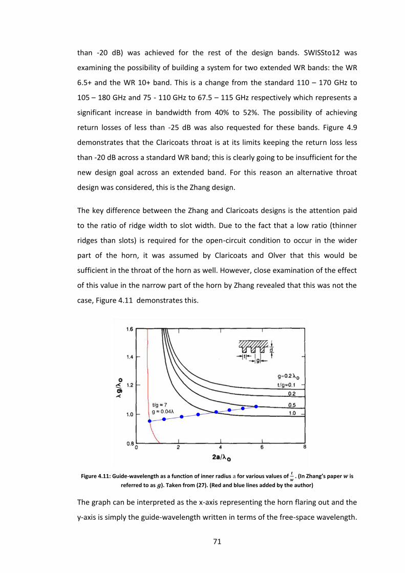
71
than -20 dB) was achieved for the rest of the design bands. SWISSto12 was
examining the possibility of building a system for two extended WR bands: the WR
6.5+ and the WR 10+ band. This is a change from the standard 110 – 170 GHz to
105 – 180 GHz and 75 - 110 GHz to 67.5 – 115 GHz respectively which represents a
significant increase in bandwidth from 40% to 52%. The possibility of achieving
return losses of less than -25 dB was also requested for these bands. Figure 4.9
demonstrates that the Claricoats throat is at its limits keeping the return loss less
than -20 dB across a standard WR band; this is clearly going to be insufficient for the
new design goal across an extended band. For this reason an alternative throat
design was considered, this is the Zhang design.
The key difference between the Zhang and Claricoats designs is the attention paid
to the ratio of ridge width to slot width. Due to the fact that a low ratio (thinner
ridges than slots) is required for the open-circuit condition to occur in the wider
part of the horn, it was assumed by Claricoats and Olver that this would be
sufficient in the throat of the horn as well. However, close examination of the effect
of this value in the narrow part of the horn by Zhang revealed that this was not the
case, Figure 4.11 demonstrates this.
Figure 4.11: Guide-wavelength as a function of inner radius for various values of
. (In Zhang’s paper is
referred to as ). Taken from (27). (Red and blue lines added by the author)
The graph can be interpreted as the x-axis representing the horn flaring out and the
y-axis is simply the guide-wavelength written in terms of the free-space wavelength.

72
In the narrow part of the horn the guide wavelength is changing very rapidly with
inner-radius, this is detrimental to return loss. However, as noticed by Zhang,
varying the ratio of ridge with to slot width produces different curves. So, similarly
to the way the slot depths were designed in Figure 4.11 by varying
it is possible
to have a much smoother change in guide wavelength, leading to a much better
impedance transformer. An example of this is shown in Figure 4.11, the red and
blue lines have been drawn over Zhang’s plot to illustrate the idea. The red line
represents the curve for a ridge-to-slot-width ratio of approximately 7 with a slot
width of approximately . The blue line with dots represents a possible
trajectory followed by a linear change in
Initial simulations were performed
following the design outlined by Zhang, i.e. beginning with a
of 7 but tapering this
over 11 periods to 0.25 instead of 0.5 following a linear trend, leading to the values
show in Table 4-4. The resulting throat geometry is shown in Figure 4.12
Table 4-4: Zhang throat ridge-width-to-slot-width ratios
Corrugation No.
1 7
2 6.38
3 5.77
4 5.16
5 4.55
6 3.93
7 3.32
8 2.70
9 2.09
10 1.48
11 0.86
12 0.25
The slots depth were also tapered in a linear fashion here, this had no effect on the
HE11 modal purity, showing that the effect of changing
dominates the
performance of the Zhang throat.

73
Figure 4.12: Zhang throat geometry
A comparison of the performance, in terms of S11 for the WR-6.5+ band is given in
Figure 4.13 for two optimized horns, one with a Claricoats and one with a Zhang
throat.
Figure 4.13: Return loss of Zhang and Claricoats throats for WR6.5+/WR6.5 bands.
Although the horn parameters (see Table 4-5 for list) are not exactly the same for
these two horns, this graph illustrates the difference between the two throats. Over
the full band the performance, in terms of S11, of the Zhang throat is superior. In the
end the variable thickness rings needed by SWISSto12 to construct the Zhang throat
were deemed too cost ineffective for mass production and the Claricoats throat was
used for all final designs.

74
4.4 Throat to aperture transition
This transition can be thought of as including the definition of the final corrugation
parameters as well as the geometry of the horn. The important quantities for the
horn’s geometry include the large aperture radius and the length of the horn. The
aperture must be large enough to ensure that the guide wavelength is close to the
free-space wavelength at this point (or in the case of the MCK it must match the
guide wavelength of a corrugated waveguide of the same diameter). The length of
the horn must provide the right taper so that there is a smooth change in guide
wavelength along the axis of the horn to provide good impedance matching and
prevent power scattering into higher order modes.
For a lot of feedhorn applications (e.g. reflector antennas) the far-field beam
pattern is of greater interest than the near-field. The application of these horns as
waveguide convertors for the MCKs however meant that the aperture fields were
just as important and, as stated in Table 4-2, they should couple strongly to a HE11
mode, as this is the desired mode of propagation in the MCK’s corrugated
waveguide.
The standard linearly tapered corrugated horn should provide the required
performance in terms of HE11 coupling, however there are other profiles worth
considering. These non-linear profiled horns are often referred to simply as “profile
horns” (30) and are defined as such when the radius of the horn as a function of the
horn’s length is a non-linear function, Figure 4.15.
There have been many profiles considered by horn designers, each with their own
advantages and disadvantages, the main positive aspects of profile horns are (30):
Linear Horn Profile Horn
Figure 4.17: Linear and Profile horns

75
1. The horn can be shorter while still having the same ratio of throat radius to
aperture radius.
2. The flare-angle at the aperture of the horn can be close to zero, this reduces
the spherical phase error.
3. The phase centre of the horn can be close to the aperture and is therefore
relatively frequency-independent.
4. The small flare angle at the throat is ideal for achieving impedance matching.
Of particular interest is point 2, the spherical phase error refers to the flatness of
the phase front at the aperture. For linear horns the phase-front is that of a locally-
spherical wave with a phase-radius given by the slant-length of the horn. The phase
error is the maximum phase difference across the aperture of the horn, it is usually
taken as the difference between the phase at the centre and edge of the aperture
and is given by (4.7), (25). Figure 4.17 shows this effect.
where is the radius of the horn and is the horn slant length. Reducing this
quantity improves the gain and efficiency of an antenna. Related to this is the phase
centre of the horn, mentioned in point 3 above. The phase centre is the position in
the horn where the beam waist is located. The beam waist is the narrowest part of
a beam, where the phase is flat, clearly is it advantageous if this is located close to
the aperture of the horn as this leads to a reduction in Frequency independence
(4.7)
Phase front
Figure 4.14: Illustration of the spherical phase front at the aperture of a horn.

76
of the phase centre position is useful for broadband designs. Some examples of
profile horn variations for corrugated horns are: Gaussian (35), Hyperbolic,
Tangential, Exponential and more (36) which can be used depending on what the
designer wants to achieve.
Not only will minimization of improve the radiation properties of the horn, but it
should also improve the coupling to a straight corrugated waveguide for the MCK
applications. A straight corrugated waveguide can be thought of as being a horn
with infinite slant length: , this leads to or a perfectly flat phase
front. For this reason a Sine-Squared profile (22) horn was examined as a candidate
for this work. The Sine-Squared profile function is described in equation (4.8) and
shown in Figure 4.15.
where is the throat radius, is the aperture radius, is the total axial length of
the horn, is the distance along the axis, is the radius at and is the degree
of the Sine-Squared profile. is a linear taper and is an extreme Sine-
Squared profile.
Figure 4.15: Sine-squared profile for various values of
The effect of using a sine-squared profile can be seen in Figure 4.16.
(4.8)
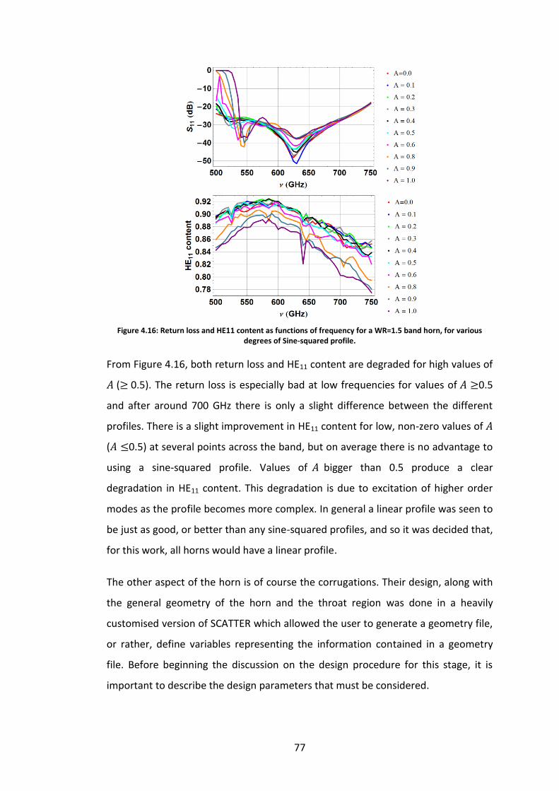
77
Figure 4.16: Return loss and HE11 content as functions of frequency for a WR=1.5 band horn, for various degrees of Sine-squared profile.
From Figure 4.16, both return loss and HE11 content are degraded for high values of
( 0.5). The return loss is especially bad at low frequencies for values of 0.5
and after around 700 GHz there is only a slight difference between the different
profiles. There is a slight improvement in HE11 content for low, non-zero values of
( 0.5) at several points across the band, but on average there is no advantage to
using a sine-squared profile. Values of bigger than 0.5 produce a clear
degradation in HE11 content. This degradation is due to excitation of higher order
modes as the profile becomes more complex. In general a linear profile was seen to
be just as good, or better than any sine-squared profiles, and so it was decided that,
for this work, all horns would have a linear profile.
The other aspect of the horn is of course the corrugations. Their design, along with
the general geometry of the horn and the throat region was done in a heavily
customised version of SCATTER which allowed the user to generate a geometry file,
or rather, define variables representing the information contained in a geometry
file. Before beginning the discussion on the design procedure for this stage, it is
important to describe the design parameters that must be considered.

78
4.5 Use of SCATTER in design process
The parameters controlling the geometry of the horn are listed in Table 4-5.
Table 4-5: Corrugated horn critical parameters
Parameter Description
This is the design frequency of the horn. It is useful to define the depth of the slots in terms of this.
This is the period of the corrugations. Chosen to be at least 3 per . =
The width of a slot.
The width of a ridge.
The ratio of ridge width to slot width is arguably more important that the values of and themselves.
The length of the horn.
This is the radius of the large aperture of the horn. Together with this defines the flare angle of the horn.
The small aperture radius.
The length of the initial section of smooth-walled waveguide.
The degree of the Sine-squared profile.
The choice of these parameters will determine the performance the horn. Once
these parameters have been defined a geometry file is then created following the
flow-chart in Figure 4.20. Is it now of interest to examine the effect of these
parameters on the performance of the horn. This is done by creating another loop
outside of the geometry file creation, which loops over a variable, termed . This
variable can be used to represent one or more of the horn geometry parameters.
The range and increment size of must be chosen appropriately for the parameter
being examined. Finally, as these horns must operate over a broad bandwidth it is
useful to perform a frequency sweep analysis. As SCATTER is a frequency domain
simulator only one frequency can be examined at a time. Usually the parametric
sweep analysis was done at three frequencies across a band: the lowest, centre and
highest frequencies. Once a design was found to be acceptable at these three
frequencies a full frequency sweep of the entire band was performed using this
design. The results of this design work are documented in section 4.8.

79
No
Set the th R( ) using (4.8), set . Set the )th R( ) using (4.8)+the th slot depth, set . Set the th length to and the )th to . Set .
Yes Is i <
No
Yes
Zhang Claricoats
Define horn parameters
Claricoats or Zhang?
Create array defining the throat slot depths and
values of
.
Create array defining the throat slot depths.
Calculate the number of sections:
Create two arrays for Radii and Lengths, set first elements as defined ( ). Set , .
Create two arrays for Radii and Lengths, set first element as defined.
Is
Finish
Set the th R( ) using (4.8), set . Set the )th R( ) using (4.8)+the th slot depth, set . Set the th length to and the )th to *. Set .
Figure 4.17: Flowchart describing how a corrugated horn geometry file was created
* For the Zhang design the first values of and are changing, after the th
they remain constant.
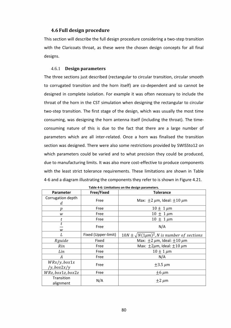
80
4.6 Full design procedure
This section will describe the full design procedure considering a two-step transition
with the Claricoats throat, as these were the chosen design concepts for all final
designs.
4.6.1 Design parameters
The three sections just described (rectangular to circular transition, circular smooth
to corrugated transition and the horn itself) are co-dependent and so cannot be
designed in complete isolation. For example it was often necessary to include the
throat of the horn in the CST simulation when designing the rectangular to circular
two-step transition. The first stage of the design, which was usually the most time
consuming, was designing the horn antenna itself (including the throat). The time-
consuming nature of this is due to the fact that there are a large number of
parameters which are all inter-related. Once a horn was finalised the transition
section was designed. There were also some restrictions provided by SWISSto12 on
which parameters could be varied and to what precision they could be produced,
due to manufacturing limits. It was also more cost-effective to produce components
with the least strict tolerance requirements. These limitations are shown in Table
4-6 and a diagram illustrating the components they refer to is shown in Figure 4.21.
Table 4-6: Limitations on the design parameters.
Parameter Free/Fixed Tolerance
Corrugation depth
Free Max: m, Ideal: m
Free m
Free m
Free m
Free N/A
Fixed (Upper-limit) Fixed Max: m, Ideal: m
Free Max: m, Ideal: m
Free m
Free N/A
Free m
Free m
Transition alignment
N/A m
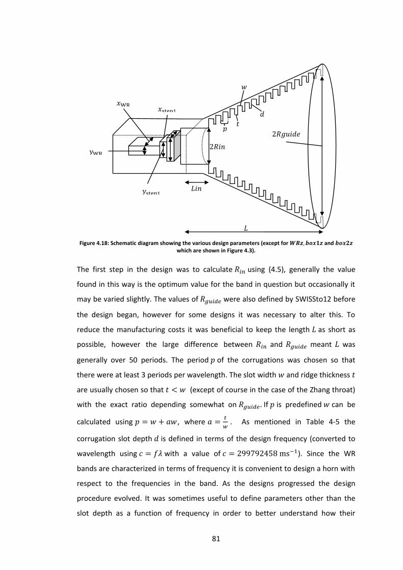
81
The first step in the design was to calculate using (4.5), generally the value
found in this way is the optimum value for the band in question but occasionally it
may be varied slightly. The values of were also defined by SWISSto12 before
the design began, however for some designs it was necessary to alter this. To
reduce the manufacturing costs it was beneficial to keep the length as short as
possible, however the large difference between and meant was
generally over 50 periods. The period of the corrugations was chosen so that
there were at least 3 periods per wavelength. The slot width and ridge thickness
are usually chosen so that (except of course in the case of the Zhang throat)
with the exact ratio depending somewhat on If is predefined can be
calculated using , where
. As mentioned in Table 4-5 the
corrugation slot depth is defined in terms of the design frequency (converted to
wavelength using with a value of ). Since the WR
bands are characterized in terms of frequency it is convenient to design a horn with
respect to the frequencies in the band. As the designs progressed the design
procedure evolved. It was sometimes useful to define parameters other than the
slot depth as a function of frequency in order to better understand how their
Figure 4.18: Schematic diagram showing the various design parameters (except for and which are shown in Figure 4.3).

82
dimensions related to the frequency band. For example was sometimes
considered as a function of . Another important change came upon the
realisation that the ratio of to was a critical parameter.
There are no exact rules or even empirical equations for choosing the values of the
parameters of a corrugated horn. Some guidelines do exist (see e.g. (22)) and make
for good starting points. However, since every horn will have a somewhat unique
application and performance criteria the method for design will be quite variable
and generally will work by trial and error (this is why simulations are of extreme
importance in this area, and fast simulations highly desirable). The key to creating a
good design in a reasonable amount of time is to choose sensible ranges when
performing parametric sweep analyses. At the beginning of this project it was quite
difficult to decide on what these ranges should be. There are some hints given in
chapter five of (22), mostly concerning cross-polarization and beam divergence
angle characteristics. There will now be a review of the performance metrics before
the specific design work is discussed in detail.
4.6.2 Performance metrics
The three main performance metrics were the peak far-field cross-polarization
levels, the return loss and the aperture-field coupling to a HE11 mode. The cross-
polarization levels are found by calculating the maximum value of the field
component perpendicular to the excitation field. The circular symmetry of the horn
makes this an arbitrary choice. The inherited SCATTER code set the -component
the co-polar direction and the -component the cross-polar direction.
Cross-polarization was the least troublesome performance metric. The return loss is
given by the matrix of the horn. The HE11 coupling is calculated by performing a
numerical overlap integral between the horn’s aperture field and an ideal HE11
mode (25). The expression for an ideal HE11 mode at the aperture of a horn is given
in (2.63), however in this case the field being coupled to is inside a straight
corrugated waveguide. A corrugated waveguide can be thought of as a horn with
infinite slant length; . This leads to (4.9):
(4.9)

83
The overlap integral for two functions:
where * indicates the complex conjugate, can be evaluated numerically using a
finite summation
where the functions are evaluated at a grid of points (with step sizes , ) over
the area of interest. Decreasing the value of the step size will better approximate
the real fields, hence increasing the accuracy of the results. A grid can be generated
using either Cartesian (as in (4.11)) or circular-polar coordinates. It is also important
to properly normalise the fields so that power is conserved and coupling is correctly
calculated. In this case it was decided to make the grid using a Cartesian coordinate
system, an example of this is shown in Figure 4.19.
Figure 4.19: Gridding system used for plotting fields/calculating coupling.
The circle in Figure 4.19 represents the aperture of the horn and along this line the
electric field must be zero. Just outside of it, in real systems there is a small electric
(4.10)
(4.11)

84
field, however for the purposes of calculating the aperture field coupling the
electric field outside the circle is set to zero, as seen in (4.12):
Since the electric fields change with transverse position in the plane, each position
in the grid is calculated independently and stored in a square array, where
the position in the array is mapped to the position in the plane of the electric field.
In (3.11) to (3.18) the and components of the electric field are written as
functions of and , so in order to grid the field using Cartesian coordinates it was
necessary to write and in terms of and , this is done using (4.13):
so that and become
and
respectively. Finally, the coupling coefficient is then
calculated as shown (4.14):
(4.14)
where is the co-polar field, is the cross-polar field and is the HE11 field.
The denominator is a normalisation factor and
. If the normalisation is
done correctly the coupling will always be between 0 and 1. It is worth noting that
only the co-polar coupling is of interest here, as the balanced HE11 mode is purely
linearly polarized, however the cross-polar antenna field must be included in the
normalisation factor to account for the total power in the aperture beam.
4.7 Example of a design (WR-1.0)
To illustrate the design process I will describe the progress of the WR-1.0 band
(750 – 1100 GHz) design. The initial parameters provided by SWISSto12 set
(4.12)
(4.13)

85
mm and mm. was calculated using (4.5) to be 0.15 mm.
Beginning with nominal values of ,
, mm the design
wavelength was varied between 0.85 1.05 ( is the central wavelength)
resulting in the plots shown in Figure 4.21 and Figure 4.25. Examining these plots it
is clear that a design with acceptable levels of peak cross-polar power (< 20 dB)
and return loss (< 20 dB) has been found (by choosing for
example), however the HE11 content at the central and upper frequency is below
the required 92 % and is almost constant with This is most likely due to the
fact that the value of is equal to between 6 and 9 wavelengths, whereas all
previous designs had been between 2 and 6 wavelengths. This was a cause for
concern as a horn with such a large aperture would be hard to keep single-moded
without being very long.
Figure 4.21: Parameter sweep of (here named 1 as a function of central frequency for the
WR-1.0 band. HE11 coupling was calculated at the centre and edges of the band. Dashed orange line shows the desired level of 92% HE11 coupling.
1 Please note the use of “ ” in place of ( ) in many of the upcoming plots.

86
This is seen in the results of Figure 4.25 as at higher frequencies more higher-order
modes have been excited than at the low frequencies. Two possible solutions were
examined: increase the length of the horn or decrease the size of the aperture, the
results of this are shown in Figure 4.26.
Figure 4.22: Parameter sweep of for the WR-1.0 band. Return loss (top) and peak cross-polar power (bottom) were calculated at the centre and edges of the band. Dashed orange lines show desired
levels of 20 dB.

87
Considering Figure 4.26, when the aperture radius is 2.5 mm, acceptable HE11
content is only achieved at lengths of over 40 mm; however at these lengths the
return loss is at -20 dB and above for 750 GHz. When the aperture radius is 2 mm
acceptable HE11 content is achieved at lengths of 30 mm and the return loss is
below -20 dB for all frequencies. Clearly the best choice is to reduce the aperture
radius to 2 mm, which was done after consulting with SWISSto12.
At this point SWISSto12 also requested that the value of
be set to unity, as the
more rings there are of the same thickness, the cheaper the horn is to manufacture
(the high frequencies in this band require very small period corrugations meaning
that many rings will be needed (hundreds) for a horn of 30 mm). Once the
parameters had been found to work at 750, 915 and 1110 GHz, a full frequency
Figure 4.23: Return loss (S11) and HE11 content as a function of length for a WR-1.0 band horn with 2.5 mm (top) and 2 mm (bottom).

88
sweep was performed and the geometry was imported into CST in order to simulate
the horn together with the rectangular to circular transition.
The results were found to vary rapidly with frequency, which lead the author to
investigate the effect of the rounding of ring radii values on the horn performance.
Up until now the values of the individual radii had been rounded to the nearest 10
m for the purposes of reducing manufacturing costs. However this was being done
after the SCATTER simulation when generating a geometry file for import to CST.
The CST simulation was then producing results that were inconsistent with
SCATTER. Quite an alarming consequence of this rounding can be seen in Figure
4.27, where 10 m precision on the radii produces a jagged geometry profile.
Figure 4.24: Comparison of 1 m and 10 m precision in radii values for the WR-1.0 horn. (Note only the first 6 mm of the total horn are shown here).

89
This clearly visible jaggedness must have a detrimental outcome on the horn’s
performance; it was decided to test this by comparing the performance with the
same horn simulated to have a realistic precision of 1 m (see Figure 4.27 for the
profile). A performance comparison for each of these rounding values is shown in
Figure 4.28 and Figure 4.29. (Note: these results were produced using SCATTER). A
more general conclusion on the effect of manufacturing tolerance as a function of
frequency is given in section 4.9.
Figure 4.25: Effects of 10 m and 1 m precision radii values on return loss (top) and HE11 coupling (bottom) as functions of frequency for a WR-1.0 band horn. (The cross-polar content was acceptable for both sets
of corrugations)

90
Figure 4.29 shows that with ring radii values rounded to the nearest m, the
designed horn meets the performance criteria (HE11, return loss and cross-polar
content) across the full WR-1.0 band (see Table 4-7 for parameters).
The values of and also have a precision of 10 m, however the performance of
the horn is not as frequency sensitive for these parameters. In this case 10 m is
equal to approximately 10 % of the slot depth and is equal to between 9 % and 10 %
of a wavelength.
Table 4-7: Final horn parameters for WR-1.0 horn. (Tolerance of 1 m required for ring radii).
Parameter Value Value ( )
971.25 GHz 1.05
0.065 mm 0.2
1 1
32 mm 98.74
2 mm 6.17
0.15 mm 0.46
1 mm 3.09
0 0
The only aspect left to be designed is the rectangular to circular transition; a two-
step transition was requested by SWISSto12. The method for designing this
transition was outlined in section 4.2.1, with the parameters being initially defined
Figure 4.26: Effects of 10 m and 1 m precision radii values on peak cross-polar power. The highest value is less than the required -25 dB for both sets of corrugations.

91
using (4.6). A parametric sweep analysis was then used to improve these values and
finally the Trust Region Framework optimization routine was used to optimize the
return loss. In this case the optimized parameters that were found are shown in
Table 4-8. This transition produced the return loss shown in Figure 4.29.
Table 4-8: WR-1.0 two-step transition, initial and final parameters.
Parameter Initial Value (mm) Final Value (mm)
0.268 0.255
0.183 0.163
0.105 0.098
0.283 0.324
0.241 0.242
0.105 0.098
Figure 4.27: Return loss for the WR-1.0 step transition.
The horn antenna was then added to the structure using a CST Visual Basic macro
file written by Stephen Doherty of Maynooth University, which reads in two text
files, one with the radii and one with the lengths and creates a series of cascaded
hollow cylinders making up the horn. This lead to the final return loss and HE11
content across the band, shown in Figure 4.29.

92
Figure 4.28: HE11 content as a function of frequency for the final WR-1.0 module
Figure 4.29: Return loss as a function of frequency for the final WR-1.0 module.
The full design met the criteria of less than -20 dB S11 and HE11 coupling greater
than 92% across the full WR-1.0 band.
4.8 Results
The preceding methods were used to design horns for 6 individual bands, including
two separate designs for the WR-3.4 band (one for the SWISSto12 module and one

93
for a plasma physics experiment at the Ecole Polytechnique Federale de Laussane
(EPFL), Switzerland, (37)). The final dimensions of the various parameters for both
the corrugated horn and step transitions are included in the following tables.
4.8.1 WR-1.0
The parameters of the horn and step-transition for the WR-1.0 band
(750-1100 GHz) are shown in Table 4-9 and Table 4-10.
Table 4-9: Two-step transition parameters for the WR-1.0 design.
Parameter Value (mm) Value ( )
0.255 0.787
0.163 0.502
0.098 0.302
0.324 1.0
0.242 0.747
0.098 0.302
Table 4-10: Corrugated horn parameters for the WR-1.0 design.
Parameter Value Value ( )
971.25 GHz 0.952
0.065 mm 0.2
1 1
30 mm 92.564
2 mm 6.17
0.15 mm 0.46
1 mm 3.09
0 0
4.8.2 WR-1.5
The parameters of the horn and step-transition for the WR-1.5 band (500-750 GHz)
are shown in Table 4-11 and Table 4-12
Table 4-11:Two-step transition parameters for the WR-1.5 design.
Parameter Value (mm) Value ( )
0.382 0.796
0.254 0.529
0.138 0.287
0.423 0.882
0.333 0.694
0.137 0.286

94
Table 4-12:Corrugated horn parameters for the WR-1.5 design.
Parameter Value Value ( )
640 GHz 0.977
0.1 mm 0.340
0.5 0.5
26 mm 58.37
2.5 mm 5.212
0.219 mm 0.457
1 mm 2.085
0 0
4.8.3 WR-3.4
The parameters of the horn and step-transition for the WR-3.4 band (220-330 GHz)
are shown in Table 4-13 and Table 4-14
Table 4-13:Two-step transition parameters for the WR-3.4 design.
Parameter Value (mm) Value ( )
0.87 0.798
0.516 0.473
0.325 0.298
0.935 0.858
0.746 0.684
0.347 0.318
Table 4-14: Corrugated horn parameters for the WR-3.4 design.
Parameter Value Value ( )
300 GHz 0.917
0.25 mm 0.229
0.4 mm 0.4
30 mm 27.519
4 mm 3.669
0.5 mm 0.459
1 mm 0.917
0 0
4.8.4 WR-3.4 EPFL
This horn was unusual as it was for use over a reduced bandwidth of 243 – 283 GHz,
and also the corrugated waveguide it was coupling to had already been built,
meaning the corrugation depths were pre-defined. However, these corrugations
were found to be non-ideal when designing the horn. The solution to this problem
was to taper the slot depths at the horn aperture to those in the waveguide over
ten periods, as shown in Figure 4.30. The parameters of the horn and step-

95
transition for the WR-3.4 band design for EPFL (243-283 GHz) are shown in Table
4-15 and Table 4-16.
Figure 4.30: WR-3.4 horn for EPFL.
Table 4-15: Two-step transition parameters for the WR-3.4 design for EPFL.
Parameter Value (mm) Value ( )
0.87 0.763
0.516 0.453
0.325 0.285
0.935 0.820
0.746 0.654
0.35 0.307
Table 4-16: Corrugated horn parameters for the WR-3.4 design for EPFL.
Parameter Value Value ( )
263 GHz 1.046
0.25 mm 0.229
0.4 0.4
81 (horn), 88 (horn+trans)
74.301
7.5 6.88
0.5 0.459
1 0.917
0 0

96
4.8.5 WR-5.1
The parameters of the step-transition and horn for the WR-5.1 band (140-220 GHz)
are shown in Table 4-17 and Table 4-18
Table 4-17: Two-step transition parameters for the WR-5.1 design.
Parameter Value (mm) Value ( )
1.304 0.783
0.89 0.534
0.437 0.262
1.48 0.889
1.246 0.748
0.499 0.3
Table 4-18: Corrugated horn parameters for the WR-5.1 design.
Parameter Value Value ( )
194 GHz 0.928
0.373 mm 0.224
0.6 0.6
48 mm 28.82
4 mm 2.402
0.75 mm 0.45
1 mm 0.6
0 0
4.8.6 WR-6.5
An interesting example of the power of a parametric sweep analysis occurred
during the design of this module. Initially a design was found to work at the lower,
centre and upper ends of the band (110, 140 and 170 GHz), (following the
procedure outlined in 4.7). However, a full frequency sweep revealed a spike in
return loss at a previously unexamined frequency (165 GHz). By reducing the
frequency range in the simulation to vary around this point (150 – 170 GHz) and
performing a parameter sweep over many frequencies (steps of 1 GHz in this case)
it is possible to find an empirical relationship between a parameter’s value and the
frequency at which the peak in return loss occurs, see Figure 4.31.

97
Figure 4.31: Return loss vs. frequency for several values of design frequency, in the WR-6.5 band.
From this information it was found that when the design frequency was equal to
approximately 0.81 times the test frequency there was a spike in the return loss at
this test frequency. So by choosing a value for design frequency which resulted in a
return loss spike outside of the WR-6.5 band’s range it is possible to remove this
spike from the band of interest. In this case the design frequency must be set to a
value greater than 145 GHz. The parameters of the step-transition and horn for the
WR-6.5 band (110-170 GHz) are shown in Table 4-19 and Table 4-20.
Table 4-19: Two-step transition parameters for the WR-6.5 design.
Parameter Value (mm) Value ( )
1.651 0.771
0.980 0.458
0.550 0.257
2.847 1.330
1.574 0.735
0.544 0.254
150151152153154155156157158159160161162163164165166167168169170-30
-25
-20
-15
-10
-5
0
(GHz)
S11 (
dB
)
S11
vs
-design 131.625
-design 132.03
-design 132.435
-design 132.84
-design 133.245
-design 133.65
-design 134.055
-design 134.46
-design 134.865
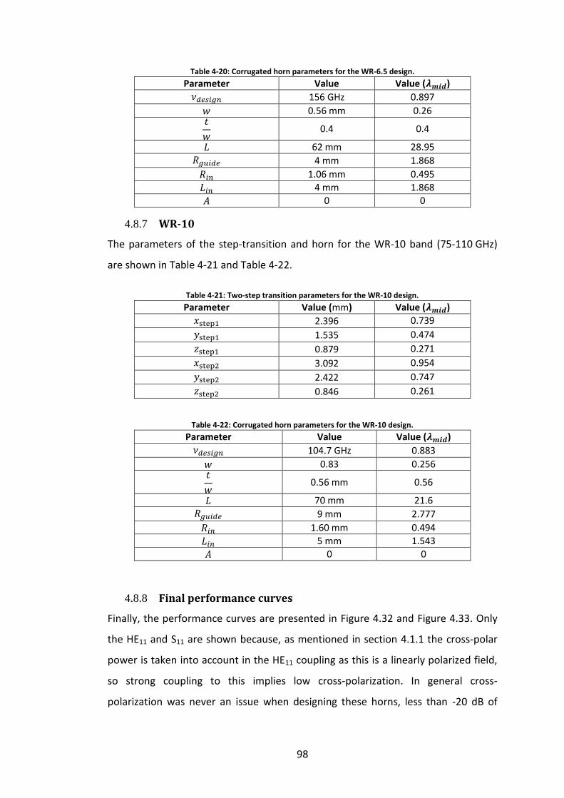
98
Table 4-20: Corrugated horn parameters for the WR-6.5 design.
Parameter Value Value ( )
156 GHz 0.897
0.56 mm 0.26
0.4 0.4
62 mm 28.95
4 mm 1.868
1.06 mm 0.495
4 mm 1.868
0 0
4.8.7 WR-10
The parameters of the step-transition and horn for the WR-10 band (75-110 GHz)
are shown in Table 4-21 and Table 4-22.
Table 4-21: Two-step transition parameters for the WR-10 design.
Parameter Value (mm) Value ( )
2.396 0.739
1.535 0.474
0.879 0.271
3.092 0.954
2.422 0.747
0.846 0.261
Table 4-22: Corrugated horn parameters for the WR-10 design.
Parameter Value Value ( )
104.7 GHz 0.883
0.83 0.256
0.56 mm 0.56
70 mm 21.6
9 mm 2.777
1.60 mm 0.494
5 mm 1.543
0 0
4.8.8 Final performance curves
Finally, the performance curves are presented in Figure 4.32 and Figure 4.33. Only
the HE11 and S11 are shown because, as mentioned in section 4.1.1 the cross-polar
power is taken into account in the HE11 coupling as this is a linearly polarized field,
so strong coupling to this implies low cross-polarization. In general cross-
polarization was never an issue when designing these horns, less than -20 dB of

99
cross-polar power came naturally with the high HE11 content. The far-field beam
patterns are shown in Appendix A, these include the cross-polar fields.
Figure 4.32: Final HE11 content as a function of frequency (normalized to the central frequency) for each of the standard WR designs.
Figure 4.33: Final S11 content as a function of frequency (normalized to the central frequency) for each of the standard WR designs.
Clearly the WR-1.5 band horn is does not meet the required level of 92 % HE11
coupling, this is due to the particular design being the first one done in Maynooth
and HE11 content was not a metric being considered at the time.

100
4.8.9 WR+ bands (WR-6.5+, WR-10+)
The possibility of producing ultra-low return loss horns (less than -25dB) across two
extended bands for WR-6.5 and WR-10 plus, as mentioned in 4.3.2, was examined.
These designs made use of the tapered transition (see 4.2.2) and the Zhang throat
(see section 4.3.2). Ultimately they were deemed too expensive for mass
production by SWISSto12. They are worth presenting as, in theory, they worked
very well. The return loss results from CST simulations are shown in Figure 4.34. The
S11 is well below -20 dB across the entire band for both designs and well below - 25
dB for most of the bands, with a large portion of both bands being below or at -30
dB, which is equivalent to 0.1% of the power being reflected.
Figure 4.34: Return loss as a function of frequency for the WR-10+ (top) and WR-6.5+ (bottom) bands using the tapered rectangular to circular transition and Zhang throat designs.
67.5 77 86.5 96 105.5 115-50
-45
-40
-35
-30
-25
-20
(GHz)
S11 (
dB
)
S11
vs Frequency for a Horn with total Length (including transisition length of 17.5mm)
of 99mm and ID = 18mm
S11
105 110 115 120 125 130 135 140 145 150 155 160 165 170 175 180-60
-55
-50
-45
-40
-35
-30
-25
-20
Frequency [GHz]
S11 [
dB
]
S11
vs Frequency (L=70 mm)
S11

101
4.8.10 Analysis of optimised geometries
An analysis of the geometries of the final designs has been done in order to try and
gain some insight to the relationships between the optimised parameters found and
the frequency band. These results may be useful for providing starting points when
designing a corrugated horn antenna using a parametric sweep analysis in the
future.
In Figure 4.35 the length of the designed horns as a function of the central
wavelength of a band is shown. From this plot it can be seen that, although the
horn length in mm generally increases with increasing wavelength, the horn length
as a function of central wavelength actually decreases.
Figure 4.35: Horn length in as a function of the central wavelength of a band.
Figure 4.36 shows the variation in
with aperture radius; here it is clear that the
value is always between 0.4 and 0.6, with no apparent trend. There is one clear
exception to this for the WR-1.0 band, where it was requested that and were
set to be equal. In Figure 4.37 the relationship between aperture radius and design
wavelength (both in terms of central wavelength) can be seen. There is a general
proportional relationship. Figure 4.38 indicates a linear relationship between
design wavelength and central wavelength i.e. as the central wavelength increases,
the design frequency gets closer to the high frequency end of a band. Finally, in
Figure 4.39 the various dimensions of the two step transition are shown as
functions of central wavelength. Clearly these values are very similar for each band,
indicating that there exists a relationship for minimal return loss (as return loss was

102
the only metric for the rectangular to circular transitions) between wavelength and
these dimensions, which is independent of the operating band.
Figure 4.36: Ratio of slot width to ridge thickness as a function of aperture radius (in terms of central wavelength).
Figure 4.37: Relationship between aperture radius and deign wavelength.
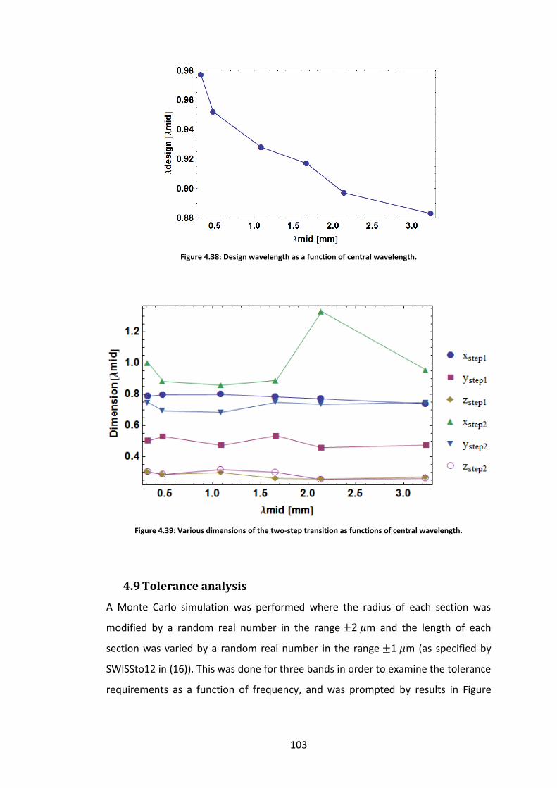
103
Figure 4.38: Design wavelength as a function of central wavelength.
Figure 4.39: Various dimensions of the two-step transition as functions of central wavelength.
4.9 Tolerance analysis
A Monte Carlo simulation was performed where the radius of each section was
modified by a random real number in the range m and the length of each
section was varied by a random real number in the range m (as specified by
SWISSto12 in (16)). This was done for three bands in order to examine the tolerance
requirements as a function of frequency, and was prompted by results in Figure

104
4.28 discussed previously. The results of such analysis are shown in Figure 4.40,
Figure 4.41 and Figure 4.42.
4.9.1 WR-1.0
The results of the tolerance analysis are shown in Figure 4.40. In this case it is clear
that m is too large a tolerance to guarantee the desired performance.
Figure 4.40: Monte Carlo tolerance analysis of the WR-1.0 band horn. The black lines are maximum and minimum values at each frequency

105
4.9.2 WR-6.5
The results of the tolerance analysis are shown in Figure 4.41. In this case it is clear
that m is an acceptable tolerance to guarantee the desired performance for
both HE11 and cross-polarization. The S11 is slightly above -20 dB at around 115 GHz
and 170 GHz.
Figure 4.41: Monte Carlo tolerance analysis of the WR-6.5 band horn. The black lines are maximum and minimum values at each frequency

106
4.9.3 WR-10
The results of the tolerance analysis are shown in Figure 4.42. In this case it is clear
that m (approximately 0.02 ) is an acceptable tolerance to guarantee the
desired performance for HE11, S11 and cross-polarization.
Figure 4.42: Monte Carlo tolerance analysis of the WR-10 band horn. The black lines are maximum and minimum values at each frequency

107
These three sets of plots demonstrate how, as would be expected, the effects of
small deviations in the corrugation parameters become more important at high
frequencies, as indicated by the increase in the black line “envelope” showing the
deviation from the average value.
4.10 Conclusions
In this chapter there has been a discussion of the methods used to design nine
corrugated feed horns. The goals of SWISSto12 for the performance of these horns
were outlined. The design was broken into three separate transition stages: the
rectangular to circular transition, the smooth-walled circular waveguide to
corrugated horn transition and the corrugated horn throat to aperture transition.
Two options for the design of the first stage were presented: firstly the step
transition, consisting of two non-standard pieces of rectangular waveguide being
placed between the WR guide and the circular waveguide, the dimensions of which
are optimised using the parameter sweep and optimization abilities of CST, and
secondly, the tapered transition, which takes a simpler approach but generates a
structure which is difficult to manufacture. The tapered transition which replaces
the two-steps of the step transition with a piece of waveguide whose cross-section
changes from being rectangular (with the WR dimensions) at the WR guide
interface to circular (with the dimension of the waveguide being coupled to) at the
circular waveguide interface. For this second type of transition the only variable to
be optimised is its length.
The second design stage again offered two general options: the Claricoats throat
and the Zhang throat. Each throat takes its name from the original designers. The
Claricoats throat uses a variable slot depth approach to form a good impedance
transformer between smooth-walled and corrugated components. It begins with
slot depths of half a wavelength at the interface and tapers these over 10 periods to
slots that are 0.27 wavelengths deep at the design frequency while keeping a
continuous flare angle. The Zhang throat also tapers the slot depths beginning at
half a wavelength and ending at a quarter wavelength, however it is done linearly in
this case. To improve the impedance transforming properties of the throat the ratio
of ridge width to slot width is also tapered, beginning with a ratio of 7 (thick ridges,

108
thin slots) and finishing with a ratio of 0.25 (thin ridges, thick slots), this is subject to
variation however depending on the aperture of the horn. The Zhang design was
considered for ultra-broadband applications (WR+ bands), however it was deemed
too difficult to manufacture and the Claricoats design was used instead, at the cost
of a reduced bandwidth.
The final stage of the design is the horn antenna itself, which was done using a
modified version of SCATTER that incorporated the generation of a geometry file.
The various horn parameters were discussed with respect to the design goals i.e if a
parameter was fixed or free. The design procedure for these parameters consists of
an educated guess of parameters and then optimizing them with a parametric
sweep analysis. As the project progressed, the author gained a better
understanding of the complex inter-relationship between the parameters and a
somewhat intuitive knowledge of sensible choices for the ranges considered for the
parameter sweeps. Even still, the design work for this stage consisted of trial and
error and continuous feed-back between parameters (finding local minima or
maxima for a parameter, trying the next parameter, then perhaps the first
parameter again etc.) until a design meeting the SWISSto12’s criteria was found.
It was only after a horn had been designed that the rectangular to circular transition
stage was designed. This was partly due to the relative speed of simulation in
SCATTER when compared with CST, but also for the practical reason that the
transition needed to couple not only to a smooth-walled circular waveguide but to a
corrugated horn.
The chosen performance metrics of the designs and how they are calculated was
discussed and the final dimensions of the horns were given and analysed in order to
identify any potential design trends.
An example of the design procedure for the WR 1.0 band horn was given. This was
followed by a Monte-Carlo analysis of the slot depths and widths and thicknesses
for the purposes of investigating manufacturing tolerances. Included in this analysis
is the effect of frequency on the tolerance requirements of a horn. It was shown

109
that (as one would expect) the tolerance requirement become more strict with
increasing frequency, reaching 1 m for the WR-1.0 band.

110
5. Measurements of WR-1.5 and WR-6.5 modules
This chapter will present results from measurements performed on several of the
horns designed as part of this work. Although seven horns/convertor-modules have
been designed to the specifications of SWISSto12, only two have been constructed
so far, these are for the WR-1.5 and WR-6.5 bands. In this chapter there will be a
discussion on the measurement results which have been received from SWISSto12
for the WR-1.5 and WR-6.5 bands and a comparison with simulation results. The
first thing to describe is the measurement facility used in all cases: the vector
network analyser.
The author would like to emphasise that he did not participate in any
measurements, had limited access to measurement data and has no knowledge of
the calibration methods or measurement set-up used. These results are preliminary
only and should be viewed as such.
5.1 The vector network analyser
Vector network analysis is a measurement technique used to accurately
characterise a device under test (DUT) by measuring its effect on the magnitude and
phase of a swept-frequency signal. These measurements are performed using a port
system similar to the one used by SCATTER, so for a two port system the DUT can be
completely characterised by the four scattering parameters and .
Consider a DUT with an incident sinusoidal signal at port 1 and a response
measured at port 2. This will lead to something like the situation in Figure 5.1:
Amplitude-ratio:
|S21|
Figure 5.1: An example of a VNA measurement of (a), a sinusoidal signal incident at port 1 and the response signal (b) at port 2.
Phase-difference: S21

111
Figure 5.1 shows how the amplitude and phase of the signal have both been
changed by the DUT. The scattering parameter is a complex number containing
information about the amplitude change and phase shift due to the DUT. In practice
both phase and amplitude can be measured by using a heterodyne system, such as
the one shown in Figure 5.2 (38).
Figure 5.2: Example of a schematic of a heterodyne measurement system used in 2-port VNA.
A radio-frequency (RF) generator sends a signal to an attenuator which controls the
total output power. From there the signal is split: one path leading to the reference
channel, the other is sent to the DUT through port 1, this port also receives
reflected signals from the DUT, which are sent to the measurement channel. The
transmitted power is received at port 2 and sent to the second measurement
channel. It is worth noting that both ports are transceivers.
So far this measurement only involves RF signals (which are easy to deal with using
standard electronics). In order to reach the THz frequencies of interest here a
frequency extension module must be used. A different frequency extension module
is necessary for each of the WR bands. The RF signal is thus applied to the frequency
extension module, where it is multiplied via frequency mixing, split and sent to the
reference channel and DUT. Before being measured this signal’s frequency is
stepped back down so that standard electronics may be used, but it still contains
the relevant information as we are only interested in changes in amplitude and
phase due to the DUT, not absolute measurements.

112
5.2 WR-1.5 module measurements
The measurements of the WR-1.5 module were carried out in Lausanne,
Switzerland by SWISSto12 using a Virginia Diodes VNA. The return loss ( ) and
radiation patterns of three stand alone (i.e. independent of the MCK) horns were
measured, and their HE11 content was characterised. The measurement system is
shown Figure 5.3 and one of the horns is show in detail in Figure 5.4.
Figure 5.3: Measurement setup at SWISSto12's lab. (39)
The return loss measurements for two horns, overlaid with CST simulation data, are
shown in Figure 5.5 where a similar trend is observed between the three data sets,
with some clear discrepancies (measurements show a lot more structure). These
discrepancies could be due to a plethora of factors such as VNA calibration, horn
manufacturing tolerance, standing waves in the measurement system (deep nulls in
the data) etc. Work remains to be done to properly account for these discrepancies.
Figure 5.4: WR-1.5 module horn (converter). Interface with WR-1.5 rectangular waveguide (left) and interface with corrugated waveguide/free-space (right).

113
Figure 5.5: Measured and simulated (CST) return loss for the WR-1.5 design. (Measurement results for C1 were not available at the time of writing)
HE11 coupling was calculated by first measuring the radiation pattern on a
10 mm 10 mm plane located 2.5 cm in front of the horn aperture, this was then
back propagated to the aperture using the diffraction integral shown in (5.1). The
results of the measurement and subsequent back propagation are seen in Figure
5.6:
Figure 5.6: Measured (left) and back propagated (right) radiation pattern from a WR-1.5 horn design.
The HE11 coupling at the aperture plane can then be calculated following the
method outlined in 4.6.2, replacing the simulated SCATTER field with the
measurement data. This is a first-order measurement and further work is required
(5.1)
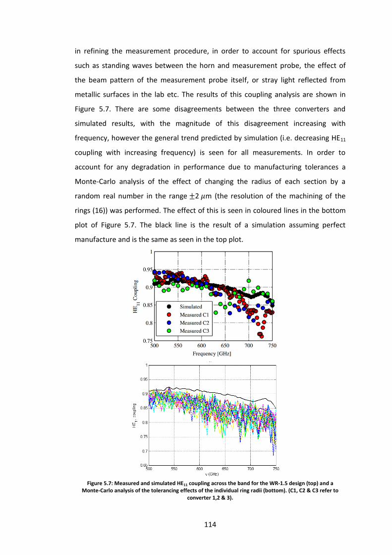
114
in refining the measurement procedure, in order to account for spurious effects
such as standing waves between the horn and measurement probe, the effect of
the beam pattern of the measurement probe itself, or stray light reflected from
metallic surfaces in the lab etc. The results of this coupling analysis are shown in
Figure 5.7. There are some disagreements between the three converters and
simulated results, with the magnitude of this disagreement increasing with
frequency, however the general trend predicted by simulation (i.e. decreasing HE11
coupling with increasing frequency) is seen for all measurements. In order to
account for any degradation in performance due to manufacturing tolerances a
Monte-Carlo analysis of the effect of changing the radius of each section by a
random real number in the range 2 m (the resolution of the machining of the
rings (16)) was performed. The effect of this is seen in coloured lines in the bottom
plot of Figure 5.7. The black line is the result of a simulation assuming perfect
manufacture and is the same as seen in the top plot.
Figure 5.7: Measured and simulated HE11 coupling across the band for the WR-1.5 design (top) and a Monte-Carlo analysis of the tolerancing effects of the individual ring radii (bottom). (C1, C2 & C3 refer to
converter 1,2 & 3).

115
The range of HE11 coupling values for realisations manufactured to a tolerance of 2
m is very similar to the measured range: The difference being around 0.05 at 500
GHz increasing to around 0.15 at 750 GHz, which is promising. However the
measurements occasionally show an increase in HE11 coupling compared to the
ideal simulations, while the Monte-Carlos analysis predicts a clear decrease. This
issue is yet to be resolved fully, but with an improved measurement procedure this
should be accounted for. Overall the measurements and simulation are showing
good agreement, indicating that tighter tolerance requirements may need to be
applied in order to reach the desired performance levels. As seen in section 4.9
these tolerance requirements are expected to be loosened for the lower frequency
bands.
Finally, a comparison was made between the measured near-field data and a CST
simulation. In order to retrieve the electric field information in CST at a plane
25 mm away from the aperture plane, a piece of vacuum 25 mm 10 mm 10 mm
was placed in front of the horn, with an electric field monitor at the end, as shown
in Figure 5.8. The results from this comparison can be seen in Figure 5.9.
Figure 5.8: CST setup for near-field calculation at a plane 25 mm from the aperture.
E-field monitor
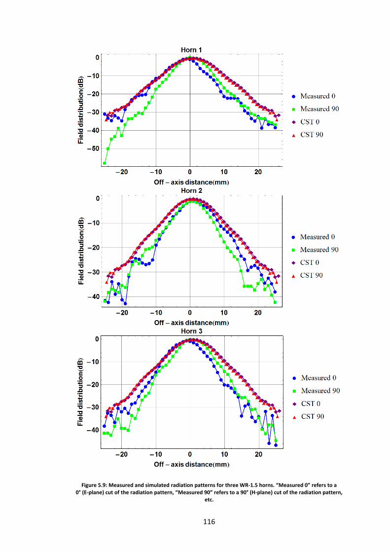
116
Figure 5.9: Measured and simulated radiation patterns for three WR-1.5 horns. “Measured 0” refers to a 0° (E-plane) cut of the radiation pattern, “Measured 90” refers to a 90° (H-plane) cut of the radiation pattern,
etc.

117
Again, there are clear differences between measurements and simulation, as well as
being due to factors outlined previously, the directionality of the measurement
probe has a large role to play in radiation pattern measurements. It is not really
measuring a single point in the field but has a beam-pattern itself which must be
considered. The author would like to reiterate the preliminary nature of these
measurements.
5.3 WR-6.5 module measurements
The WR-6.5 module has so far only been considered for use with the Material
Characterisation Kit (MCK) and so no radiation pattern measurements have been
performed, meaning that the HE11 coupling has yet to be measured. However both
the return loss and insertion loss have been measured, again this was done by
SWISSto12 in Lausanne.
5.3.1 WR-6.5 return loss
The return loss measurements for two manufactured horns are shown in Figure
5.10, including the simulated results from CST. Again there are major disagreements
between the data sets, especially in terms of the peaks and nulls, these are likely
caused by similar factors outlined in section 5.2. The overall levels however are in
general agreement, with the measured data largely remaining below the – 20 dB
requirement.
Figure 5.10: WR-6.5 antenna return loss measurements and CST simulation.

118
5.3.2 WR-6.5 insertion loss
Insertion loss is the loss in transmitted power, not caused by reflections. The
general mechanism for insertion losses in the case of a corrugated horn such as
those considered here is Ohmic losses due to the finite conductivity of the antenna
walls; the rapidly varying electric and magnetic fields induce eddy-currents in the
walls leading to Joule heating, thus power is dissipated in the form of heat. This is
another reason it is desirable to contain as much power as possible on axis in the
horn, as there will then be less power available at the walls to create these eddy-
currents.
The insertion loss results are shown in Figure 5.11, again including measurements
and simulation. The insertion loss measurements were performed by placing a
reflector at the aperture of the antenna and measuring the S11 on a VNA. In this
setup if the antenna was made from PEC it would be expected that all power would
be reflected and the S11 should be at 0 dB across the band. Any deviation from this
is due to the insertion loss.
Figure 5.11: Insertion loss measurements for two horns. Better time-gating parameters were chosen for the top plot. Better insertion loss was recorded for the bottom plot. No CST simulation data is available here due
to limited computational resources at the time.
The insertion loss is worse at the low frequencies for Antenna 2 here due to some
of the rings not being manufactured properly by SWISSto12’s supplier. The
measured data here appears quite noisy, this is because of the way the
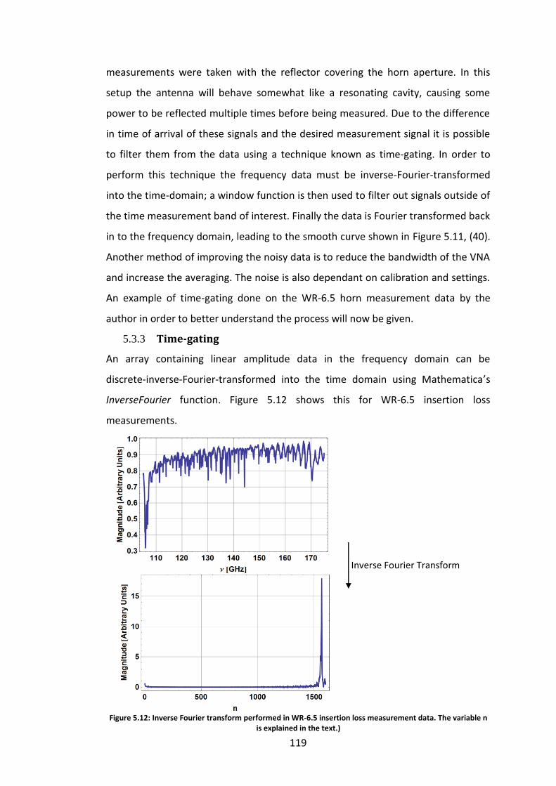
119
measurements were taken with the reflector covering the horn aperture. In this
setup the antenna will behave somewhat like a resonating cavity, causing some
power to be reflected multiple times before being measured. Due to the difference
in time of arrival of these signals and the desired measurement signal it is possible
to filter them from the data using a technique known as time-gating. In order to
perform this technique the frequency data must be inverse-Fourier-transformed
into the time-domain; a window function is then used to filter out signals outside of
the time measurement band of interest. Finally the data is Fourier transformed back
in to the frequency domain, leading to the smooth curve shown in Figure 5.11, (40).
Another method of improving the noisy data is to reduce the bandwidth of the VNA
and increase the averaging. The noise is also dependant on calibration and settings.
An example of time-gating done on the WR-6.5 horn measurement data by the
author in order to better understand the process will now be given.
5.3.3 Time-gating
An array containing linear amplitude data in the frequency domain can be
discrete-inverse-Fourier-transformed into the time domain using Mathematica’s
InverseFourier function. Figure 5.12 shows this for WR-6.5 insertion loss
measurements.
Inverse Fourier Transform
Figure 5.12: Inverse Fourier transform performed in WR-6.5 insertion loss measurement data. The variable n is explained in the text.)

120
From this it is clear that in the time domain there is a sharp impulse response, this is
caused by the first round-trip reflection of the signal, there are several smaller
ripples around this peak, these are caused by the secondary reflections, and it is this
effect that we want to remove. Before discussing how this is done, it is worth noting
that the independent variable of the bottom plot in Figure 5.12 ( ) is in terms of
time “bins” rather than units. In order to convert this to units of seconds we must
use (5.2), leading to Figure 5.13.
where is the number of data points and is the measurement step size.
Figure 5.13: Inverse Fourier transform of WR-6.5 measurement data, in terms of time.
In order to remove the unwanted time signals we can implement a window
function. A window function is essentially a way of reducing data outside of the
region of interest to zero. There are many window functions available, which all
have associated advantages and disadvantages depending on the scenario. A
standard window function is the Hann or Hanning window, given in equation (5.3),
which is taken from (41). A plot of a Hanning window is shown in Figure 5.14.
where, is the width of the window in terms of samples.
(5.2)
(5.3)

121
Figure 5.14: Hanning Window, N=150.
This function will have the effect of smoothly reducing the data around the peak to
zero, clearly the width of the window (determined by the choice of ) will have an
important impact on the effectiveness of the window function. Care must also be
taken to align the window to the correct region of the data set. A window function
can be applied to the data using (5.4), (41). That is, multiply the two functions and
perform a discrete Fourier transform.
where, is the width of the window in terms of samples. Multiplying this window
by the data shown in Figure 5.12 (lower plot) with leads to Figure 5.15.
There are clearly still some ripples at the higher end of the scale, due to the
asymmetry of the time response. Now, Fourier transforming this back into the
frequency domain leads to Figure 5.16.
Figure 5.15: Comparison of raw data from Figure 5.12 with the same data after multiplication by the window function.
(5.4)

122
Figure 5.16: Time-gated data (red) overlaid on measured data (blue). The orange lines mark the edges of the WR-6.5 band.
The time-gated data is clearly smoother than the raw data with much of the
variations due to multiple reflections removed. Increasing the measurement
sampling rate or investigating other window functions could improve this technique
further.
The raw data with overlaid time-gated data curves for both antennas are shown in
Figure 5.17 and Figure 5.18.
Figure 5.17: Raw and time-gated data for Antenna 1.
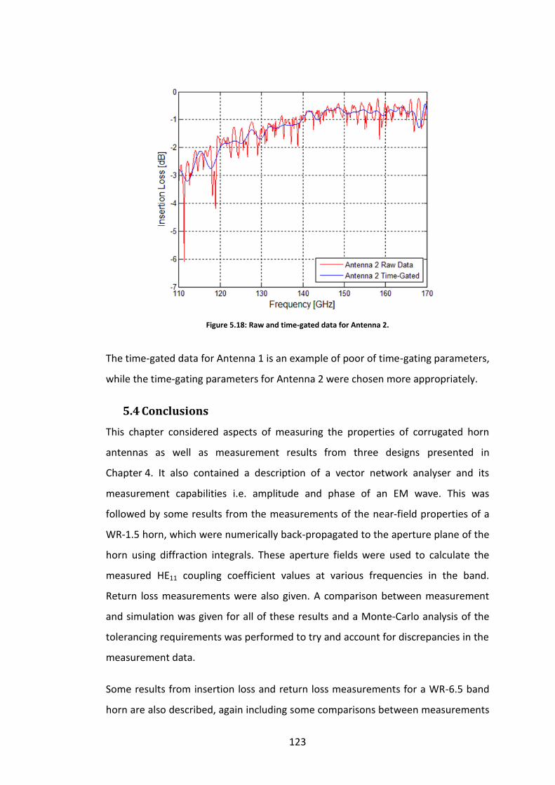
123
The time-gated data for Antenna 1 is an example of poor of time-gating parameters,
while the time-gating parameters for Antenna 2 were chosen more appropriately.
5.4 Conclusions
This chapter considered aspects of measuring the properties of corrugated horn
antennas as well as measurement results from three designs presented in
Chapter 4. It also contained a description of a vector network analyser and its
measurement capabilities i.e. amplitude and phase of an EM wave. This was
followed by some results from the measurements of the near-field properties of a
WR-1.5 horn, which were numerically back-propagated to the aperture plane of the
horn using diffraction integrals. These aperture fields were used to calculate the
measured HE11 coupling coefficient values at various frequencies in the band.
Return loss measurements were also given. A comparison between measurement
and simulation was given for all of these results and a Monte-Carlo analysis of the
tolerancing requirements was performed to try and account for discrepancies in the
measurement data.
Some results from insertion loss and return loss measurements for a WR-6.5 band
horn are also described, again including some comparisons between measurements
Figure 5.18: Raw and time-gated data for Antenna 2.

124
and simulation for the return loss measurements which were in good agreement.
There was also an explanation and example of time-gating on the insertion loss
measurements.

125
6. Final summary and conclusion
This thesis was primarily concerned with the development of high-performance
corrugated conical horn antennas for use in the THz region of the electromagnetic
spectrum. They are fed by a smooth-walled circular waveguide which transition to
an industry standard WR-band rectangular waveguide for use in vector network
analysis experiments (VNA). These antennas will be built by the company
SWISSto12 and will serve the dual purpose of acting as free-space radiators or as
crucial components in SWISSto12’s material characterisations kits (MCK), where
they bridge the gap between the VNA frequency extension module rectangular WR-
band guides and a cylindrical corrugated waveguide containing a sample for
measurement.
Chapter 1 was an introduction to THz radiation, with some context given to its place
in the electromagnetic spectrum and how we must borrow techniques from the
microwave and optical regions to manipulate and model it. The many applications
of THz were mentioned with emphasis on astronomical applications and security
and medical imaging. The research interests of SWISSto12 were discussed in some
detail, and the novelty of their ‘stacked ring’ approach to building corrugated
waveguides was described. The utilization of these waveguides in plasma physics
experiments and in SWISSto12’s own MCK was also outlined and the role of the
author in designing the horn antenna components for these kits was detailed.
Another innovative manufacturing process used by SWISSto12 for building
inexpensive high-quality passive elements (stereolithography (3D printing)
combined with a metallic plating technique to create light-weight waveguide and
smooth-walled horn antennas) was then described.
Chapter 2 contained a description of the operation of circular and rectangular
waveguides, including a derivation of the circular TE and TM modes. The use of
waveguides as horn antennas was introduced followed by the concept of hybrid
modes and the importance of the HE11 mode in particular. I showed how the
relative contribution of TE11 and TM11 modes propagating in a guide can be adjusted
to minimize levels of cross-polar power. Two methods for generating a HE11 mode

126
were outlined, these were the Potter horn and the corrugated cylindrical
waveguide.
Chapter 3 contained the analysis methods used in this thesis for the design of
waveguides and corrugated conical horn antennas. These were: the surface
impedance model (including the hybrid mode model), the mode-matching
technique for corrugated horns, which was employed in the in-house software
package SCATTER, and the finite integration technique as used by the commercially
available simulation software CST: Microwave Studio. Examples from SWISSto12
horns and the Planck telescope were used to illustrate the techniques.
Chapter 4 described the design process for the horn components which were a
major element of this work. The design requirements were outlined (HE11, S11 and
cross-polar content) and the design process was broken into three stages. These
were: the rectangular to circular transition, the circular to corrugated transition and
the corrugated waveguide to free-space/large-diameter corrugated waveguide. Two
possible types of transition for the rectangular to circular (two-step or smooth) and
circular to corrugated (Claricoats or Zhang) sections were outlined. The important
elements to consider when designing a corrugated horn antenna, such as the
geometric-profile and period of corrugations were discussed. Next the full design
procedure was described, including the method of parametric sweep analysis for
designing a corrugated horn and the specific performance metrics and how they
were calculated. An example of a design for the WR-1.0 band was given next. This
was followed by the final design parameters for each of the horns (WR-1.0, WR-1.5,
WR-3.4, WR-3.4 for EPFL, WR-5.1, WR-6.5, and WR-10) and a presentation of the
final return loss and HE11 content. The requirement of HE11 content greater than
92% across the band was met for all of the designs apart from the WR-1.5 band. The
WR-1.5 design was the first one developed, and this was before HE11 content had
become a critical factor. The return loss requirement of less than -20 dB across the
band was also realised for each band except the WR-6.5 which rises above this
value at two spots in the band at around 122 GHz and 168 GHz. The S11 for two
ultra-low return loss horns designed for the WR-6.5+ and WR-10+ bands was then
shown, with a value below -25 dB across the bands. An analysis of the geometries of

127
the horns and step transitions was performed in order to find possible trends which
may be of use to future designers and the results of this were presented with
several trends identified. These trends include a relationship between horn length
and the central wavelength of a band, a small range of optimum values for the ratio
of slot width to ridge width for each of the designs, a linear relationship between
design wavelength and central wavelength and also fairly constant relationship
between the dimensions of the step-transition and central wavelength of a band.
Finally an examination of the effect of manufacturing tolerances of the ring radii on
the performance of the horns using a Monte Carlo analysis was presented for three
of the WR-bands, showing how the tolerance requirements increase with
frequency. A tolerance of 2 m was acceptable for the WR-6.5 and WR-10 bands,
however it was not good enough to guarantee the desired performance for the WR-
1.0 band.
Some measurements of the horns which have been built so far were discussed in
Chapter 5, which began with a description of a VNA. The measured return loss and
HE11 content of the WR-1.5 band horn as well near-field radiation patterns at three
frequencies across the band were compared with SCATTER and CST simulations,
showing good agreement. The return loss measurements for the WR-6.5 band horn
were also compared with simulation and show good agreement as well. The
insertion loss measurements were shown and the procedure of time-gating on
these was described using an example.
In conclusion: 9 individual corrugated conical horns with rectangular to circular
transitions were designed to meet the criteria set by SWISSto12 (HE11 coupling,
return loss and cross-polarization), and the components which have been
manufactured and measured so far show promising performance.
6.1 Future work
Some potential future work will now be considered. The code used during the horn
design process could be implemented as a starting point to build a general horn
design programme with a user interface, where the user specifies some
requirements for the horn’s performance (e.g. bandwidth, gain, peak cross-polar

128
power, Gaussicity, HE11 content, return loss, side-lobe level, etc), restrictions on its
geometry and a parameter to be swept over or optimized. This would be a very
useful tool which would speed up the design process.
There currently exist two versions of SCATTER: one for cylindrical waveguides and
one for rectangular waveguides, however there is no way to combine them. Such a
combination would allow for design of the rectangular to circular transitions in
SCATTER, speeding up the simulation time compared to CST. The irregular shaped
boundary at the rectangular-circular interface prevents closed-form solutions to the
power coupling integrals at this plane, i.e. we cannot analytically solve the power-
coupling integrals between a rectangular and circular mode-set. It can be solved
analytically but this takes longer than a CST simulation. However, by transforming
from a surface integral to a line integral along the edge of the boundary it may be
possible to match or even improve on the speed of CST. This is one of the current
projects at Maynooth University.
Finally, only two of the designs (WR-1.5 and WR-6.5) in this thesis have been built
and tested. Further work on the measurement procedure for forthcoming horns will
provide more accurate results on their modal content, return loss and radiations
patterns etc.

129
7. Bibliography
1. C. O' Sullivan, J. A. Murphy. Field Guide to Terahertz Sources, Detectors and
Optics. Bellingham : SPIE, 2012.
2. Coherent Manipulation of semiconductor quantum bits with terahertz radiation.
B. E. Cole, J. B. Williams, B.T. King, M.S. Sherwin, C.R. Stanley. 2000, Nature, Vol.
410, pp. 6 0- 63.
3. Tranmission Line Technology for Electron Cyclotron Heating. J. L. Doane. 1, 2008,
Fusion Scence and Technology, Vol. 53, pp. 39 - 53.
4. High Field Dynamic Nuclear Polarization- The Renaissaince. R. G. Griffin, T. F.
Prisner. 2010, Physical Chemistry Chemical Physics, Vol. 12, pp. 5737 - 5740.
5. Searching for Terahertz Waves. X. C. Zhang. 9, London : Nature, 2010, Nature
Photonics, Vol. 4, p. 662. ISSN - 1749-4885.
6. Materials for Terahertz Science and Tecnhology. B. Ferguson, X. C. Zhang. 14,
2002, Nature Materials, Vol. 1, pp. 26 - 33.
7. Plasmonics: Superfocusing of Terahertz Waves. M.B.Johnston. 1, London :
Nature, 2007, Nature Photonics, Vol. 1, pp. 14-15. ISSN - 1749-4885.
8. Security Applications of Terahertz Technology. M. C. Kemp, P. F. Taday, B. E. Cole,
J. A. Cluff, A. J. Fitzgerald, et al. Orlando : SPIE, 2003. Terahertz for Military and
Security Applications. Vol. 5070, pp. 44 - 52. ISBN - 9780819449290.
9. Herschel Mission Overview and Key Programmes. G. L. Pilbratt. San Diego : SPIE,
2008. Space Telescopes and Instrumentation: Optical, Infrared, and Millimeter. Vol.
7010, pp. 1-12. ISBN - 9780819472205.
10. Herchel Spce Observatory. [Online] [Cited: 5th August 2015.]
http://www.herschel.fr/cea/star-formation/en/.

130
11. M. Whale. Optical Characterisation of Astronomical Submillimetre Receivers
including ALMA Bands 5 and 9. Maynooth : National University of Ireland,
Maynooth, PhD thesis, 2010.
12. Attacama Large Milimetre Array. [Online] [Cited: 17th August 2015.]
http://www.almaobservatory.org/en/visuals/images/astronomy/?g2_itemId=3431.
13. Planck Collaboration. Planck 2015 results. XIII. Cosmological Parameters. Ithica :
ArXiv, 2015.
14. European Space Agency. [Online] [Cited: 12th August 2015.]
http://www.esa.int/spaceinimages/Images/2013/03/Planck_CMB.
15. Teraview. [Online] [Cited: 17th August 2015.]
http://www.teraview.com/applications/index.html.
16. Note: Stacked rings for terahertz-wave guiding. E.de Rijk, A. Macor, J-Ph.
Hogge, S. Alberti, J-Ph. Ansermet. 6, Melville : AIP Publishing, 2011, Review of
Scientific Instruments, Vol. 82.
17. SWISSto12. [Online] [Cited: 10 December 2015.]
http://www.swissto12.ch/Products/Material%20Characterisation%20Kit/index.html
.
18. Note: Three-dimensional stereolithography for millimetre wave and terahertz
aplications. A. Macor, E. de Rijk, S. Alberti, T. Goodman, J.P. Ansermet. 4, Melville :
AIP Publishing, 2012, Review of scientific instruments, Vol. 83.
19. P. C. Magnusson, Andreas Weisshaar, Vijai K. Tripathi, Gerald C. Alexander.
Tansmission Lines and Wave Propogation, Fourth Edition. London : CRC Press, 2001.
20. N.J. Cronin. Microwave and Optical Waveguides. London : Institue of Physics
Publishing, 1995.

131
21. D.Jackson. Fourier Series and Orthogonal Polynomials. [book auth.] Dunham
Jackson. Fourier Series and Orthogonal Polynomials. Oberlin : The Mathematical
Association of America, 1941, p. 86.
22. P.J.B Claricoats, A.D.Olver. Corrugated horns for microwave antennas. London :
Peter Peregrinus Ltd, 1984.
23. P. D. Potter. A New Horn Antenna with Suppressed Sidelobes and Equal
Beamwidths. Pasadena : Internal Report: NASA, Jet Propulsion Laboratory, 1963.
24. Characterization of a Dual-Mode Horn for Submillimeter Wavelengths. H. M.
Pickett, J. C. Hardy, J. Farhoomand. 8, New York : IEEE Publishing, 1984, IEEE
Transactions on Microwave Theory and Techniques, Vol. 32, pp. 936 - 937. ISSN:
0018-9480.
25. P. F. Goldsmith. Quasioptical Systems. New York : Institue of Electrical and
Electronic Engineers, 1998.
26. CST - Computer Simulation Technology. CST-Computer Simulation Technology
Web Site. [Online] [Cited: 07 September 2015.] https://www.cst.com/.
27. Design of Conical Corrugated Feed Horns for Wide-Band High-Frequency
Applications. X. Zhang. 8, New York : IEEE Publishing, 1993, Transactions on
Microwave Theory and Techniques, Vol. 41, pp. 1263-1274.
28. R. Colgan. Electromagnetic and quasi-optical modelling of horn antennas for far-
IR space applications. Maynooth : National University of Ireland Maynooth, Ph.D
Thesis, 2001.
29. E. Gleeson. Single and multi-moded corrugated horn design for cosmic
microwave background experiments. Maynooth : National University of Ireland,
Maynooth, PhD Thesis, 2004.
30. A.D. Olver, P.J.B. Claricoats, A.A.Kishk and L. Shafai. Microwave Horns and
Feeds. New York : IEEE Press, 1994.

132
31. Optical modelling offar-infrared astronomical instrumentation exploiting
multimode horn antennas. C. O'Sullivan, J. A. Murphy, I.McAuley, D. Wilson, M. L.
Gradziel, N. Trappe, F. Cahill, T. Peacocke, G. Savini, K. Ganga. Montreal : SPIE,
2014. Millimeter, Submillimeter, and Far-Infrared Detectors and Instrumentation
for Astronomy VII. Vol. 9153.
32. Discrete Electromagnetism with the Finite Integration. M. Clemens, T.
Weiland. : Progress in Electromangetics Research, 2001, Progress in
electromagnetic research, Vol. 32, pp. 65-67.
33. S.Doherty. Optical and Quasi-Optical Design and Analysis of Astronomical
Instrumentation including a Prototype SAFARI Pixel. Maynooth : National University
of Ireland, Maynoth, Ph.D Thesis, 2012.
34. Analysis of TE11 - to HE11 Corrugated Cylindrical Waveguide Mode Convertors.
G. L. James. 10, New York : IEEE Transactions on Microwave Theory and Techniques,
1981, IEEE Transactions on Microwave Theory And Techniques, Vol. 29, pp. 1059 -
1066.
35. Improved Radiation Pattern Perfromance of Gaussian Profiled Horn Antennas. R.
Gonzalo, Jorge Teniente and Carlos del Rio. 11, : IEEE Transactions of Antennas
and Propagation, 2002, IEEE Transactions on Antennas and Propagation, Vol. 50, pp.
1505-1513.
36. Profile Options for Feed Horn Design. C. Granet. Sydney : IEEE, 2000. Microwave
Conference, 2000 Asia Pacific. pp. 1448-1451.
37. Personal Communication with SWISSto12.
38. E. McLoughlan. Optimisation of a Near Field Scanning Syatem. Maynooth :
National University of Ireland, Maynooth, Masters Thesis, 2012.
39. Rectangular to Large Diameter Conical Corrugated Waveguide Converter Based
on Stacked Rings. S. Doherty, A. von Bieren, F. Cahill, A. Macor, E. de Rijk, N.

133
Trappe, M. Billod, C. O'Sullivan. Lisbon, 2015. European Conference on Antennas
and Propagation (EuCAP).
40. Rohde & Shwartz. 1EZ44: Time Domain Measurements using Vector Network
Analyzer R&S®ZVR. : Rohde & Shwartz, 1998. .
41. R. G. Lyons. Understanding Digital Signal Processing. Reading, Massachusetts :
Addison-Wesley Publishing Company, 1997.
8. Appendix A
Presented here are the far-field beam patterns for the 6 horns designed for the
standard WR bands.

134
Figure A.1: Far field beam patterns for the WR-1.0 horn at 750GHz (top), 925GHz (middle) and 1100GHz (bottom).

135
Figure A.2: Far field beam patterns for the WR-1.5 horn at 500GHz (top), 625GHz (middle) and
750GHz (bottom).

136
Figure A.3: Far field beam patterns for the WR-3.4 horn at 220 GHz (top), 275 GHz (middle) and
330 GHz (bottom).
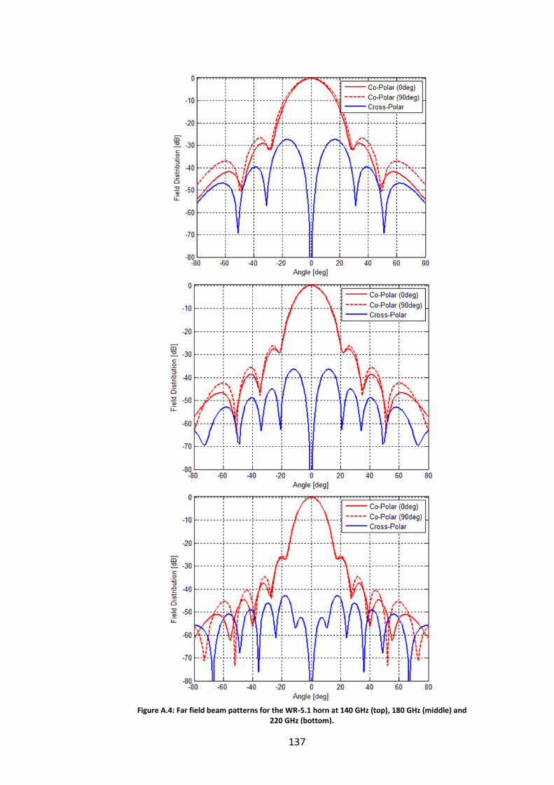
137
Figure A.4: Far field beam patterns for the WR-5.1 horn at 140 GHz (top), 180 GHz (middle) and 220 GHz (bottom).

138
Figure A.5: Far field beam patterns for the WR-6.5 horn at 110 GHz (top), 140 GHz (middle) and 170 GHz (bottom).

139
Figure A.6: Far field beam patterns for the WR-10 horn at 67.5 GHz (top), 91.25 GHz (middle) and 115 GHz (bottom).


![Performance of IBA New Conical Shaped Niobium [18O] Water ... · Vienna sept 2010, poster #9, session P13. Table 2: Results Summary Conical 6 Conical 8 Conical 12 Conical 16 Insert](https://img.dokumen.tips/doc/110x75/5f901a7319a03054823be5c3/performance-of-iba-new-conical-shaped-niobium-18o-water-vienna-sept-2010.jpg)


![N ElectroScience Laboratory · ElectroScience Laboratory ... Horn antennas Corrugated horns, , ,. Antenna gain ... D 2 2 (3) from the horn aperture [1]](https://img.dokumen.tips/doc/110x75/5b69914d7f8b9af23e8e504e/n-electroscience-electroscience-laboratory-horn-antennas-corrugated-horns.jpg)