On conical horn antennas

Koop, H.E.M.; Dijk, J.; Maanders, E.J.

Published: 01/01/1970

Document VersionPublisher’s PDF, also known as Version of Record (includes final page, issue and volume numbers)

Please check the document version of this publication:

• A submitted manuscript is the author's version of the article upon submission and before peer-review. There can be important differencesbetween the submitted version and the official published version of record. People interested in the research are advised to contact theauthor for the final version of the publication, or visit the DOI to the publisher's website.• The final author version and the galley proof are versions of the publication after peer review.• The final published version features the final layout of the paper including the volume, issue and page numbers.

Link to publication

General rightsCopyright and moral rights for the publications made accessible in the public portal are retained by the authors and/or other copyright ownersand it is a condition of accessing publications that users recognise and abide by the legal requirements associated with these rights.

• Users may download and print one copy of any publication from the public portal for the purpose of private study or research. • You may not further distribute the material or use it for any profit-making activity or commercial gain • You may freely distribute the URL identifying the publication in the public portal ?

Take down policyIf you believe that this document breaches copyright please contact us providing details, and we will remove access to the work immediatelyand investigate your claim.

Download date: 16. Jul. 2018

ON CONICAL HORN ANTENNAS

by

H.E.M. Keep, J. Dijk and E.J. Maanders

i

Technische Hogeschool Eindhoven

Eindhoven Nederland

Afdeling Elektrotechniek

Eindhoven University of Technology

Eindhoven The Netherlands

Department of Electrical Engineering

On Conical Horn Antennas

by

H.E.M. Koop, J. Dijk and E.J. Maanders

T.H. Report 70 - E - 10

February 1970.

Contents.

List of principal symbols

Summary

ii

2. !h~_~2~E~~E~_!i~1~_~!_~_£~~i£~1_h~E~_~~~~~~~' 2.1. Introduction.

i.2. Vector potentials.

2.2.1. The magnetic vector potential.

2.2.2. The electric vector potential.

2.3. The principle of duality.

2.4. The vector potential in a spherical coordinate system.

2.5. The field components in spherical coordinates for an arbitrary field.

2.6. The field components within an infinite long conical waveguide with circular cross-section.

2.7. Characteristics of conical waveguides.

2.B. The fields in the transmission region.

2.9. Comparison of circular waveguides and conical horns.

2.10 Conclusion.

3.1. Introduction.

3.2. General considerations on the approximations.

3.3. Approximations for well matched horns.

3.4. The theory of Fresnel zones.

3.5. Final conclusions.

Appendix A. Coordinate transformations.

Appendix B. Vector analysis.

Appendix C. Bessel functions.

Appendix D. Legendre functions.

Page

iii

iv

J.

2. I .

2. 1 •

2. ).

2.2.

2.3.

2.3.

2.4.

2.8.

2.9.

2. 12.

2. 18.

2.21.

2.23.

3. I.

3. I.

3.2.

3.5.

3.6.

3.8.

4. I.

AI.

BI.

CI.

DI.

iii

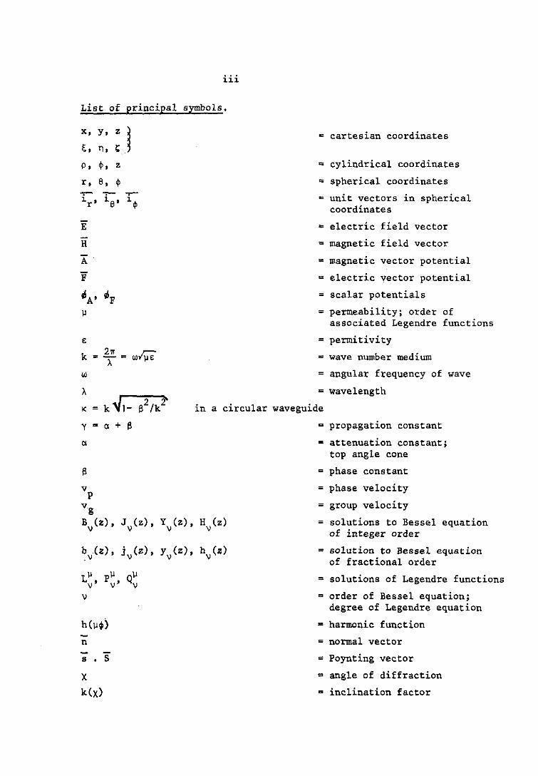
List of principal symbols.

x, y,

~. n. P. ~. z

r. e. ~

i r • i e• i~

2" ~ k = T = w>').Io

W

= cartesian coordinates

= cylindrical coordinates

= spherical coordinates

= unit vectors in spherical coordinates

= electric field vector

= magnetic field vector

= magnetic vector potential

= electric vector potential

= scalar potentials

= permeability; order of associated Legendre functions

= permitivity

= wave number medium

= angular frequency of wave

= wavelength

K = in a circular waveguide

y = a + a a

v p

v.g Bv(z). Jv(z). Yv(z). Hv(z)

b(z). j (z). y (z). h (z) .v v v v

n

s S

x k(X)

= propagation constant

= attenuation constant; top angle cone

= phase constant

= phase velocity

= group velocity

= solutions to Bessel equation of integer order

= solution to Bessel equation of fractional order

= solutions of Legendre functions

= order of Bessel equation; degree of Legendre equation

= harmonic function

= normal vector

= Poynting vector

= angle of diffraction

= inclination factor

iv

Summary

This report comprises a fundamental study of the near fields

of a conical horn antenna. For this purpose the field components

of the conical horn are deduced from Maxwell's equations.

It appears that it is possible to approximate the aperture

field of a finite conical horn antenna from the fields within

an infinite conical horn.

From the radiating antenna aperture the fields outside the

antenna can be computed and compared with the various measuring

results.

In this way a clearer insight is obtained into the usual

approximations which are related to the flare angle and the

length of the horn.

-1-

1. Introduction

Horn antennas are well known as primary radiators for large

parabolic antennas. Recently the conical horn antenna has

become more popular in large reflector antennas owing to

its properties of symmetry. The formulae concerning the

properties of conical horn antennas with relation to their

aperture field are mostly approximations. Most authors

(refs. 14, 15) indicate that the aperture field of a conical

horn antenna is similar to that of a circular waveguide but

with spherical wavefronts. It is further explained that the

approximations are valid if the flare angle of the conical

horn is small and the horn itself long. Mostly, further

information with regard to the length of the horn and the

limitations of the flare angle is not available. It is the

purpose of this paper to investigate the expressions used

and the influence of small flare angles and large apertures.

Therefore, in Section 2 the field equations within the conical

horn are deduced from Maxwell's equations, using electric

and magnetic vector potentials. It is further investigated

what requirements are to be made on the horn parameters in

order that the aperture field may be represented by fields

of a circular waveguide with spherical wavefronts.

The near field radiation pattern of the horn antenna is

discussed in Section 3 and especially the equation

-jkr e r

• dS,

referred to by several authors (refs. 13, 14, 15), using the

zone construction of Fresnel.

This report comprises part of the graduate work of Koop (ref.19).

-2.1-

2. The aperture field of a conical horn antenna

An antenna is capable of maximum power transfer if the radiation impedance

equals that of free space, viz. 120w ohms. In microwave engineering it is

common practice to use horn antennas with a diameter much longer than the

wavelength. In that case boundary effects may be neglected if the

radiation impedance of the antenna equals that of free space.

In this chapter we shall discuss how the dimensions of a conical horn

antenna are to be chosen so that it is well matched to free space.

We will also discuss the aperture ,fields of a conical horn antenna, to see

under what conditions the aperture fields can be approximated by the

fields of a waveguide with circular cross-section but with spherical wave

fronts.

2.2 Vector potentials

In a homogeneous source-free region with the restriction of time dependence

to the time factor ejwt , the field will satisfy the following Maxwell

equations:

V x E + jw~H - 0

V xH - jWEE • 0

V.E • 0

V.H • 0

These equations can be solved by introducing vector potentials. Any

d~vergenceless vector is the curl of some other vector; therefore,

as V.H • 0

H • V x A ,

where A is called a magnetic vector potential.

(2.1)

(2.2)

(2.3)

(2.4)

(2.5)

-2.2-

In the same way the electric field E can be represented by

E=-'i'xF ,

In analogy with A the quantity F is called the electric vector

potential. It is also possible to represent the field by a

combination of both vector potentials A and F. Part of the field

will be expressed in A, the remaining part in F (ref. 1).

Substituting Eq. (2.5) in (2.1) we obtain

'i' x (E + jWIlA) = 0 •

Any curl-free vector is' the gradient of some vector, hence

(2.6)

(2.7)

E = - jW\lA - 'i'~A (2.8)

where ~A = ~A(x,y,z) is an arbitrary electric scalar potential.

Substituting (2.5) and (2.8) in (2.2) gives

= -

the frequently encountered parameter k

the wave number of the medium.

211 - -= A

W~ and is called

Depending upon the coordinate system used, a value of A has been

chosen, in such a way that the simplest solution of Eq. (2.9) is

obtained. For rectangular coordinates, this equation becomes by

a vector identity

- 2-'i'('i'.A) - 6A - k A - - jWE'i'~A

i \ For cartesian' coordinates the best choice appears to be

simplifying Eq. (2.9) to

6A + k2A - 0 •

(2.9)

(2.10)

(2.11 )

-2.3-

This equation is known as the Helmholtz equation or complex wave

equation.

From Eq. (2.2) and Eq. (2.6) it is readily found that

H = - j wEF - Il~F '

where 4p is an arbitrary electric potential. If Eq. (2.6) and

Eq. (2.12) are now substituted in Eq. (2.1) we obtain

- 2-11 x 11 x F - k F = - j WII Il4p

being similar to Eq. (2.9).

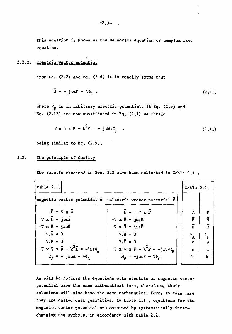
2.3. The principle of duality

The results obtained in Sec. 2.2 have been collected in Table 2.1 •

(2.12)

(2.13)

Table 2.1. Table 2.2.

magnetic vector potential A electric vector potential F

H = 11 x A E = - 11 x F A

11 xHm jWEB -11 x E = jWIIR E

-11 x E = j WIIR 11 xR= jWEB H

Il.E - 0 '7.R = 0 ~A '7.R - 0 '7.B = 0 E

- 2- 11 x F _ k2F = -jwlI'7\-'7 x '7 x A - k A - -jWE~ X '7 A II E = ;.. jWIIA - '7~A ~ = -jwEF - '7~F A k

As will be noticed the equations with electric or magnetic vector

potential have the same mathematical form, therefore, their

solutions will also have the same mathematical form. In this case

they are called dual quantities. In table 2.1., equations for the

magnetic vector potential are obtained bY'systematically inter­

changing the symbols, in accordance with table 2.2.

F

H

-E

~F

II

E

k

-2.4-

It is often convenient to divide a problem into two dual parts.

For example, the Maxwell equations can be regarded as a super­

position of the equations derived in Sec. 2.2.1 and Sec. 2.2.2;

let EA and HA be the fields belonging to A and ~ and ~ the

fields belonging to F, then the following equations are obtained:

E = EA + EF H = H A +~

'V x H = A jwd;A 'V x fA = jW\.IHA

'V x~= jW8EF -'V x E = F jw\.I~

The total solution, being the superposition of the two partial

solutions, becomes:

E -'V x F I x 'V xA • + -.- 'V JW8 (2. 14)

- I xF H· 'V x A + -.- 'V x 'V JW\.I (2.15)

Depending upon the purpose we can carry out the calculations in

the case of F = 0 and A t 0 or F t 0 and A = 0

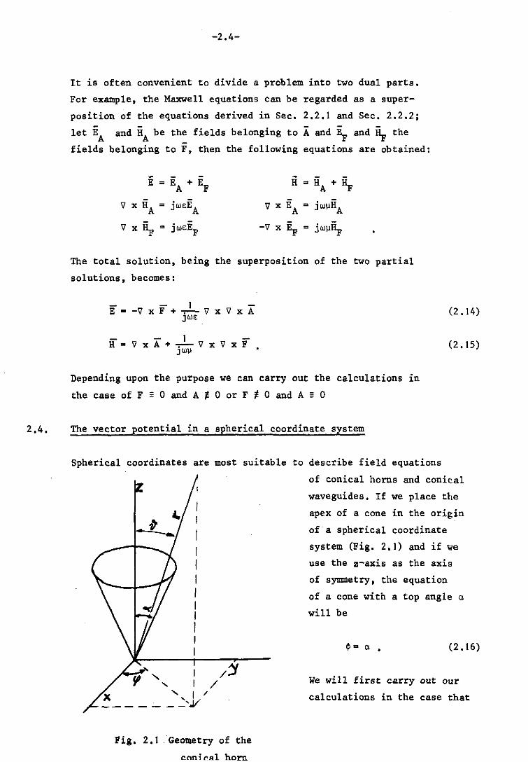
2.4. The vector potential in s spherical coordinate system

Spherical coordinates are most suitable to describe field equations

X " I / _______ '.J/

/:1 /

Fig. 2. I . Geometry of the

enn; l'!.Rl horn.

of conical horns and conical

waveguides. If we place the

apex of a cone in the origin

ofa spherical coordinate

system (Fig. 2.1) and if we

use the z-axis as the axis

of symmetry, the equation

of a cone with a top angle a

will be

-¢'= ex • (2.16 )

We will first carry out our

calculations in the case that

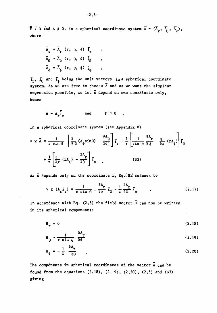
-2.5-

F ,i 0 and A to. In a spherical coordinate system A - (Ar , "e' Aq,)'

where

A = A (r, El, 41) .,.

r r 1y

As = A ~

(r, a, 41) Ie - - (r, 41)

.,. Aq, = Aq, El, 141

~, :is and Iq, being the unit vectors in a spherical coordinate

system. As we are free to choose A and as we want the simplest

expression possible, we let A depend on one coordinate only,

hence

A = A T r r

and F - 0

In a spherical coordinate system (see Appendix B)

'J x A = r sin e5 [~a (Aq,sina) - ::6] Ir + ~ [Si~ e ::r - ;r (rAq,~ Ie

1 ~a aArJ -+ - - (rA ) - - i r a]:" El ae 41 (B3)

As A depends only on the coordinate r, Eq.(B~ reduces to

In accordance with Eq. (2.5) the field vector H can now be written

in its spherical components:

H - 0 r

aA H r - , ar-e r S1n e

1 aA Hq, -

r r ae

The components in spherical coordinates of the vector A can be

found from the equations :(2.18), (2.19), (2.20), (2.5) and (B3)

giving

(2.17)

(2.18)

(2.19)

(2.20)

-2.6-

(V x V x A) __ .,.;..--" r ~J -r r sin e La e l

a2A (V x V x A) e =

r

(V x V x A) <I> = r sin e .

We are now able to solve Eq. (2.9) if the quantity V~A is also

written in its spherical coordinates. For that case we will use

equations found in Appendix B:

1 a~A + r Te Ie + r sin

If we substitute the equations (2-.21), (2.22), (2.23) and (B. I),

the e and <I> components will give rise to the following equations

= -

and

The quantity ~A is still an arbitrary scalar ~q. (2.8)]. If we

take

aA . ~ r

- JWE"A = 'at

the equations (2.24) and (2.25) be~ome identities. If we substitute

(2.21 )

(2.22)

(2.23)

B. I)

(2.24)

(2.25)

(2.26)

- 1 in Eq. (2.9) the equation E a ~ V x H and use for ~A the Eq. (2.26), JOlE

it is readily shown that

E -...L fa2

Ar + k2A 1 (2.27) r JOlt l-;tT rJ

The e and <I> components of the field vector A can be derived

immediately from the equations (2.22) and (2.23) as E = ...L V x V x A JOlE

giving

(2.28)

(2.29)

-2.7-

Expanding Eq. (2.9), if we use the r component of Eq. B.I for

the scalar 4>A (ref.I, p.267) and Eq. (2.21), the r component

of Eq. (2.9) becomes

This equation represents the scalar Helmholtz equation for

spherical coordinates and it can be shown that the equation

is equivalent to

6. -'II + iiJJ = 0 , A A

A where IJiA = ~ is a solution of the Helmholtz equation.

The Helmholtz equation ,in spherical coordinates in o/A' namely

I a { 2 aijl A I I zar r Tr of. 2 . r' , r Sl.n

can be solved using the method of separation of variables, if we let

'/IA

c R(r) H(EI) ~(4)) •

This method has been described elsewhere (ref.l. p.265) giving

the following trio of separated equations:

~ and ~ being separation constants.

Eq. (2.33) is related to the Bessel equation. The solutions are

(2.30)

(2.31 )

(2.32)

(2.33)

(2.34)

(2.35 )

-2.8-

called spherical Bessel functions with an arbitrary solution bv(kr)

related to cylindrical Bessel functions by

Eq. (2.34) is related to the Legendre equation with the solution

LIl cos e v

Eq. (2.35) has ha~onic solutions like cos Il~, sin Il~, e jll¢, e-jll¢, etc., or commonly named h(Il~). If Ar = r~A we have solutions such as

Ar = krbv (kr). L~ cos e. h(Il$)

A possible choice will be (see also Appendices C and D),

The same procedure can be followed if A = a and F In accordance with the duality principle we shall

= Fr. r r find in that

case that E - O. We may draw here the conclusion that these r

waves are TE to r. In the same manner the equations (2.18) to

(2.20) prove - T -that A • Ar1r' and F = a gives waves TM to r.

2.5 Field components in spherical coordinates for an arbitrary field

Generally A • Ar~ and F • Fr~' In the case that both Hr t a

and Eta, we choose A so that it satisfies:

(App.C)

(App.D)

(2.36 )

(2.37)

r 1 r a2Ar r .2 J

Er • jWE ~ ar2 + k Ar (2.27)

In the same way we choose Fr to satisfy the dual equation of Eq. (2.27+

viz. ,

[ 2 J a F 2

H • ...L ~+kF r J Wll . 2 r

3r

(2.38)

-2.9-

We can now tabulate all the field components which are the sum

of a TM and a TE field expanding Eqs.(2.14) and (2.15)

E =....!... [a 2

Ar + k2AJ

(ref.I,p.269) •

r jWE ar2 r

H = -.I-l· a2Fr + k2F]

r JWJl ar2 r

aF r I

r sin e ~ + -.--JWJlr

aA + _._1_

a2F He

r r = sin r e aq, JWEr 3r ae

I aF a2A Eq,

r r = - Te + jWEr sin ar. a~ r e

aA r

-- + r ae

If A exists and F = 0, the field will be TM to r; if A 1 0 r r r and F exists, the field will be TE to r.

r

2.6 The field components within an infinite long conical waveguide

with circular cross-section

(2.39)

(2.40)

(2.41)

(2.42)

(2.43)

(2.44 )

The field equations which have been deduced in the previous sections

can very well be used to calculate the fields within a circular

conical waveguide. For this purpose we will consider the field

components of a wave which is propagated in the direction r for

r > O.

First some modifications to the solution supplied by Eq. (2.37) of

the differential equation (2.9) are introduced.

The harmonic solution h (Jlq,) can only exist if Jl is an integer.

The solution is still arbitrary if we choose Jlmm and m > O.

A further simplification might be achieved, if the coordinates

are taken in such a way

The arbitrary solutions

that h(mq,) = sin mq,.

of the Legendre equation Lm (cose) can \i

be further limited if we notice that Lm (cose) should be finite \)

.-2.10-

for 0 < 0 < n. In that case (see App. D)

m m Lv (cos 0) = Pv ( cos 0),

where v can be found from the boundary conditions.

Finally, as we consider long distances r, where a travelling

wave in direction r should be present,

b (kr) = h(2) v v (kr) , being a Hankel function

of the second kind (App. C).

A possible solution for A and Fr will be r

A = CA • kr . h (2) (kr) pm (cos 0) sin m~ r v v

F -CF·kr. h (2) (kr) pm (cos 0) sin m~ r v' v'

where v is found from the boundary conditions for

and v' from the boundary conditions for TE waves. r

, TM waves r

Using recurrence relations for br (kr) (see Appendix C3.5), we

. find that

:x rbv (X)]= bv (x) + xb' (x) v .

If Eqs. (2.47) and (2.48) are used in combination with the

Eqs. (2.39) to (2.44), we find the following field components

for TM waves

E ·C '.1('.1 + 1) r - -J A w£r

H • 0 r

h(2) (kr) pm (cos 0) sin m~ v v

(2.45)

(2.46)

(2.47)

(2.48)

(2.49)

(2.50)

E • jCA

k~in 0 fh (2) (kr) + k.r h (2)' (kr~ pm' (cos 0) sin m~ e w£r L v v· IJ V (2.51)

mit (2) m He • CA sin 0 hv (kr) Pv (cos 0) cos m~ (2.52)

-2. J J-

H~ CA k sin e h(2) (kr) m' (cos e) sin m~ = Pv v (2.54 )

For TE waves we will find

E = 0 r (2.55)

H = -jC v' (v' + J) h (2) (kr) pm (cos e) sin m<j> r F Wllr v' v' (2.56 )

Ee = -C mk h (2) (kr) pm (cos e) cos m~ F sin e v' v' (2.57)

= j~ . ksin e He -F wllr

fh (2) (kr) LV' + kr h(2)' (ke)] pm'

v' v I (cos e) sin m<j>

(2.58)

E~ = -CF

k sin e h (2) (kr) pm: (cos e) sin m~ 't' 'V 1 V

(2.59)

H = -jC ~ F

mk Wllr sin e [h~~) (kr) + kr h~~)' (kr) ] p~, (cos e) cos m~

(2.60)

The boundary conditions can be found assuming that the waveguide

boundary is a perfect conductor. These conditions require that

the tangential component of the electric field vanishes at the

boundary. Therefore, there will be no tangential electric field

component at the surface of the horn or E~ = 0, and consequently

the boundary condition for TM waves will be

pm (cos e)e = 0 'V ._(1

and for TE waves

rd m @0 Pv' (cos e)] = -S=a m'

sin a Pv' (cos a)

(2.6 J)

(2.62)

-2.12-

2.7 Characteristics of conical waveguides

In this section some characteristic quantities of conical waveguides

will be discussed, to obtain a clearer insight into the physical

behaviour of the fields within a conical waveguide. Partly the

w9rk of Barrow and Chu (ref. 2) and Schorr and Beck (ref. 3) will

be dealt with in this section as well.

The propagation constant for exponentially propagated waves

y m a + S , where av is the attenuation constant and Sv the v v v phase constant, may be defined as the logarithmic rate of decrease

of magnitude and of change of phase

y = v - -u au a - - In u ar - ar

where u represents any component of the field and the wave is

propagated in the direction r.

It can be proved (ref. 2) that for increasing r where r » A, the

phase constant Sv and approaches k.

The phase velocity v and the wavelength "h of the waves within - p 2w

horn are given _~y vp = w/Sv and "h(u,r) = Sv group velocity v is given by v = dw/dS • g g v

the

the

The

by

characteristic wave impedance in the radial direction is given

Z (r) v

From the Eqs. (2.49) to (2.60) it is readily seen that Z is v

independent of e and ~ but it is a function of the cone angle a and

the mode v.

It is common practice (ref. 4) to distinguish 3 regions in which

y (u,r) and Z (r) have a different behaviour. v v In the region kr « v + i the phase constant s« ~w but it

increases rapidly with r until it approaches the value 2; which

is the phase constant in free space. The group· velocity is very

low, almost zero. Therefore the signal will be propagated at a

low velocity. The waves have apparently a hybrid character,

being a mixture of standing and travelling waves (ref. 2).

(2.63)

(2.64)

-2.13-

This region is often called the attenuation region.

The wave impedance is mainly inductive for TE waves and

capacitive for TM waves. If r is increased, the real part

of Zv increases as well, while the imaginary part decreases.

It has been found by Schorr and Beck (ref. 3) that the wave

impedance in the attenuation region can be approximated by

Z E == v,

Z M':::' V'

f¥. [ 11' (2v + 1)

E Lv r (v + !) • r (v

'- 11' (2v

lr (v + D + 1)

3 r (v + '2)

r being the gamma function as explained elsewhere (ref. 51 6.1.6).

Within the region kr .::::. v+i the impedance becomes more real.

Bucholtz (ref. 4) has calculated for TE waves and kr = v+!

,ru fret) (6 ~} . ]-1 Zv,E<': vf· 2~(}) • \V+!} (j - h) - vtr ,

where

(2.65 )

(2.66 )

For our purpose the transmission region kr » v+l is most important.

The behaviour of the waves in this region approaches asymtotically

to that of travelling waves in free space.

If r decreases, and consequently the radius of the horn increases,

the influence of the walls of the cone becomes smaller.

For both TM-and TE waves the wave impedance approaches to ~_(ref.4) and

the propagation constant

y m a + je 1 - - + jk r

. 1 -jkr if the field 4S expressed as u = - e • r

For a finite horn with a length rh for which krh » v+l the fields

near the aperture do not differ much from the fields at the aperture

-2.14-

of an infinitely long horn. The horn has a wave impedance

which is nearly equal to that of free space and is said to

be well matched to free space.

The quantities mentioned above have only significance if

the field varies harmonically with increasing r; this means

that the opening angle should not be too large ( < 400 ••• 500

).

If the wall of the conical waveguide has a finite conductivity,

the effect of this is greater in the attenuation region than

in the transmission region. This is explained by Barrow and Chu

(ref. 2), who indicate that the power dissipated in the walls

of the horn is approximately proportional to the square of the

tangential magnetic field strength at the wall. For the same

amount of transmitted power, this magnetic field is much larger

in the attenuation region than in the transmission region, and

so power loss is also greater.

Consequently, the curves of the attenuation constant a as a

function of radial distance will be steeper for practical horns

than for ideal horns with a perfect conductivity (ref;Z, p.56).

We will now determine the above characteristics by ·using the

equations (Z.49) to (2.60) for the wave impedance for TE and TM

waves. We find

z -j ~ ~l • ,~2)' (k,' r1

= \I,E £kr h (2) (kr) \I

and

Z ~ t'- · h~2)' (kr) 1 = h (2) (kr) \I,M J 8 'kr

\I

It is readily seen that

Z Z = ~ E • M • v, v, r;...

These expressions for the wave impedance depend on \I but can be

used for any different flare angle.

From Eqs. (2.49) to (2.60) expressions are also to be found for

the propagation constant y.

(2.68)

(2.69)

(2.70)

-2.15-

Eqs. (2.49), (2.52) and (2.54) for TM waves and (2.56), (Z.57)

and (Z.59) for TE waves will lead to the propagation constant

h(Z)' (kr) y =':k _v:""",--,-_

I,v h(Z) (kr) v

while Eqs. (Z.51) and (Z.53) for TM waves and Eqs. (Z.58) and

(2.60) for TE waves result in a different propagation constant

l~ (2) (2) ~~ !- I h (x)+xh (x) ax x v v

x=kr

In all cases Eq. (Z.63) has been used.

Eq. (Z.72) can be simplified by realising that (see also App. C 47)

a U 1 I + xb' (x) I a2 (xb (x» - -(b (x)+xb' (x) = - - (b (x) + ---

axxv v Z v x axZ v v x

= - ~ (bv(x)+xb~(x) + bv(X)(V(V ; I) I) x x

Therefore,

-{~. L, = or YZ, v

I -v( v + I)

2 Y • k I x -+

h (2) ( ) 2,v x I v x -+~ x h 2 x)

=kr v

As will be noticed from Eqs. (2.68), (2.69) and (2.74), the

behaviour of Z and Y is mainly determined by the factor v v

(2) , h (x)

1. + ~vT.<'<""-_ x h(2) (x)

v x=kr

(2.71 )

(Z.72)

(Z.73)

(2.74)

This factor can be simplified in accordance with the method followed

in Appendix C (Sec. 3.6) to

-2.16-

1 -+ 2x x=kr

which approaches for x » I and x » V to -j. (Appendix C3.6).

Therefore Zv and

if the following

y will approach their free space values v

conditions are fulfilled:

(kr)2» v 2 for Y2,v

kr » v for Z v,E ' Z M and Y I , v \I,

and kr » I for Y1,v' Y2,v' Z v,E and Z v,M

Bucholtz (ref. 4) derives complicated expressions for ZEin v, the attenuation region, the transmission region and also in

the region'kr ~ v+!. The equations are not mentioned here as they are not used any

further. Interesting, however, is the dependence of the real and

imaginary part of Z E as a function of v. v, Once values have been found for Z E' it is not difficult to v, find values for Z Musing Eq. (2.70). v, It will be proved in this chapter that the conical horn is well

matched to free space if kr » v for the highest mode we want

to use,

The mismatch is readily found by using the expression of Bucholtz

for Z if kr + ~: v,E

Z'V120rr v,E

'V 120 rr ~ +

(2v + I) 2 - 1

8(kr)2

] , v and: kr being large

If the mismatch should not increase by 1% it is readily seen that

the minimum length of the horn should be at least

r. > (v + !>>. m~n

(2.75)

(2.76)

(2.77)

-2.17-

The requirements with regard to the matching of the horn to free

space are not the only factors to be considered when dimensioning

a horn.

Very important is also the required beamwidth, which is in close

relationship with the aperture (ref. 6, p.193).

Mostly no problem arises if small beamwidths are required, but

if the aperture should be smaller than is advisable for correct

matching, attention should be paid to the method of Geyer (ref.7).

He surrounded the horn edge by one or more conducting collars

which act as short-circuit quarter wavelength stubs. It appears

that in this case the mismatch of the horn decreases considerably.

-2.18-

2.8 The fields in the transmission region

In this section the fields in the transmission region are

calculated for the case that the flare angle is small and

the distance from the fieldpoint to the apex is large. This

is done to enable .the field in the aperture of a conical

horn to be compared with a conical waveguide.

We will give only relations for TE waves.

If TM waves are required they may be readily found by means

of the duality principles.

We will consider the equations (2.55) to (2.60) and introduce

some modifications. If the flare angle a of the cone is small

and the distance r from the fieldpoint to the apex is large we

can write, in accordance with Appendix D.5,

and

~ pm (cos e) = - sin e pm' (cos e) a de v v

e 2J + O(sin '2)

where

~ - (2v + 1) sin i e

and

~' - ~ - (v + i) cos 1 e

Further,

sin2

1e - 1 [1 - coseJ - 1 [1 - 1 + 1i - k e4

+ ..... J 2 0

2 - (ie) [1 - 0 (; 2) J

(2.78)

(2.79)

(2.80)

(2.81)

(2.82)

-2.19-

Even for e = 200 the error in Eqs. (2.78) and (2.79) is not more

than 3% (See also Appendix D.3). Substitution of the results

obtained here in the Eqs. (2.55) to (2.60) yields in the following

field equations for the TE waves:

m

Hr = -jCF v'(~~;I) h~~) (kr) [-(v'+O cos ie] Jm

t(2v'+I) sin !e} sin m~

(2.83)

m

Ee = -CF stu e h~7)(kr) [ -(v'+O cos !e] J m {(2v'+I) sin Ie} cos m$

(2.84 )

m+1

E,p = -CF k h~~)(kr) l-(v'+o cos ie] Jm

{(2v'+I) sin !e} sin m$

H =­e Ep

Z , E v ,

H = Ee <jl Z, E v ,

From Appendix C it is explained that

h~2) (kr) • ~ [je-j(x- ~) + 0 (~/~)l x=kr

If we use this relation, Eqs. (2.84) and (2.85) may be written as

E • CM 1 J L (2v'+I) sin ie] -jkr

e cos m<jl e

, m and

E = CM 2 Jm r (2v'+I) sin ieJ

. -jkr <jl S1n m<jl e ,

(2.85 )

(2.86)

(2.87)

(App.C.35)

(2.88)

(2.89)

-2.20-

where, assuming that a is small and. kr large,

(2.90)

and

m m ~,1 = -~,2 -s"'in=-e~- (,,'+1> cos !e

= -c M,2 2 (cos I e) (2,,'+1) sin Ie

m

K're

In Eq. (2.91) K' is by definition

1 K' = -- (2,,'+1) sin !e re

which for small e turns into

It is also possible to determine values for" and ,,' from the

boundary conditions.

From Eq'. (2.61) and (2.78) we find for TM waves

or

P~ (cos a) • [-(,,+!) cos m

!a] . J {(2"+1) m

J {(2v+1)sin!a}-o,asa<; m

sin !a} = 0

th If we call (2,,+1) sin!a - Emn' Emn will represent the n

zero point of the function J (x). For every value of E there m mn will be a value of ". Therefore we obtain as boundary value

for the TM mode mn,r

(2.91 )

(2.92)

(2.93)

(2.94)

If the flare angle a is

boundary conditions for

and (2.79) or

resulting in

-2.21:-

small v will.be large. , mn TE waves are found using

E' - d v' = d sinia mn

th ,

where E' is the n zero point of Jm (x). mn

In the same way

the Eqs. (2.62)

2.9 Comparison of circular waveguides and conical horns

The field expressions for waves in circular waveguides are

found in several textbooks (ref. 6) and will therefore not

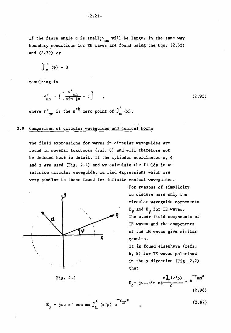
be deduced here in detail. If the cylinder coordinates p, ~

and z are used (Fig. 2.2) and we calculate the fields in an

infinite circular waveguide, we find expressions which are

very similar to those found for infinite conical waveguides.

For reasons of simplicity

(2.95)

we discuss here only the

circular waveguide components

x \

Fig. 2.2

, -y z E - jW\l K' cos m~ J (K'p) e mn ~ m

E p and Etp for TE waves.

The other field components of

TE waves and the components

of the TM waves give similar

results.

It is found elsewhere (refs.

6, 8) for TE waves polarised

in the y direction (Fig. 2.2)

that

E = p

-y z e mn

(2.96)

(2.97)

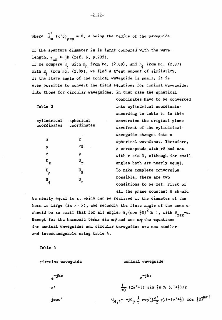
-2.22-

, where J (K' p) = 0, a being the radius of the waveguide.

m pea

If the aperture diameter 2a is large compared with the wave­

length, Ymn ~ jk (ref. 6, p.20S).

If we compare E with E from Eq. (2.88), and E~ from Eq. (2.97) p e ~

with E~ from Eq. (2.89), we find a great amount of similarity.

If the flare angle of the conical waveguide is small, it is

even possible to convert the field equations for conical waveguides

into those for circular waveguides. In that case the spherical

Table 3

cylindrical coordinates

z

p

~

U z

U p

U~

spherical coordinates

r

re

~

U r

Ue

U~

coordinates have to be converted

into cylindrical coordinates

according to table 3. In this

conversion the original plane

wavefront of the cylindrical

waveguide changes into a

spherical wavefront. Therefore,

p corresponds with re and not

with r sin e, although for small

angles both are nearly equ~l.

To make complete conversion

possible, there are two

conditions to be met. First of

all the phase constant a should

be neariy equal to k, which can be realised if the diameter of the

horn is large (2a » A), and secondly the flare angle of the cone C<

should be so small that for all angles 8, (cos 1e)2 ~ I, with e =C<. max

Except for the harmonic terms sin m<f and cos m<f the equations

for conical waveguides and circular waveguides are now similar

and interchangeable using table 4.

Table 4

circular waveguide

-jkz e

jWJlK '

conical waveguide

-jkr e

(2\1'+1) sin !e ~ (\I'+!)/r re

-2.23-

2.10 Conclusion and final remarks

It has been proved in the previous sections that if the dimensions

of a conical horn meet certain requirements, it is possible to

prescribe the aperture fields of a conical horn by means of the

modes of a circular waveguide, however, with a spherical wavefront.

The requirements which the horn has to meet can be given only

roughly.

(I) The flare angle should be small, i.e.

2 (cos la) ~ I

although according to AppendixD (Sec. 3) this requirement

is not very severe.

(2) The length of the horn should meet two requirements, viz.

Ikrh » I and

which means that the diameter of the horn (2a) should be large

compared with IA.

It is advised to calculate the error for various values of a and vh

'

preferably by means of a computer.

The phase centre of conical horns with a small flare angle fed by

a circular waveguide is not situated in the cone's apex. If a is

made smaller, the phase centre will move toward the aperture.

If a = 0, in the case of circular waveguides the phase centre is

situated in the aperture. If the horn is very short and the aperture

diameter small, it even appears that the phase centre is located in

front of the aperture outside the horn (ref. 18). At the junction

of the circular waveguide and the cone higher modes are excited

but rapidly attenuated. Schorr and Beck (ref. 3) have even calculated

the length of the journey of higher modes in the attenuation region.

-3.1-

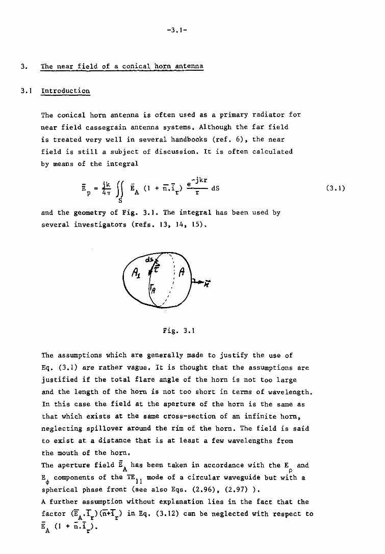
3. The near field of a conical horn antenna

3.1 Introduction

The conical horn antenna is often used as a primary radiator for

near field cassegrain antenna systems. Although the far field

is treated very well in several handbooks (ref. 6), the near

field is still a subject of discussion. It is often calculated

by means of the integral

Ep = * Jl EA S

-jkr e --dS

r

and the geometry of Fig. 3.1. The integral has been used by

several investigators (refs. 13, 14, 15).

Fig. 3.1

The assumptions which are generally made to justify the use of

Eq. (3.1) are rather vague. It is thought that the assumptions are

justified if the total flare angle of the horn is not too large

and the length of the horn is not too short in terms of wavelength.

In this case the field at the aperture of the horn is the same as

that which exists at the same cross-section of an infinite horn,

neglecting spillover around the rim of the horn. The field is said

to exist at a distance that is at least a few wavelengths from

the mouth of the horn.

The aperture field EA has been taken in accordance with the E and

E~ components of the TEll mode of a circular waveguide

spherical phase front (see also Eqs. (2.96), (2.97) ).

p but with a

A further assumption without explanation lies in the fact that the

factor (EA.T) Gi+T) in Eq. (3.12) can be neglected with respect to r r

EA(l+n.i).

(3. I)

-3.2-

It appears that Eq. (3.1) gives results which very well agree

with measured values. The assumption that the phase centre is

situated at the apex of the cone of the horn is not true in

all cases; it appears that if the flare angle becomes very small,

the phase centre moves towards the aperture. In the case that

the flare angle is zero, the phase centre is situated in the

aperture plane (ref. 6, P. 343).

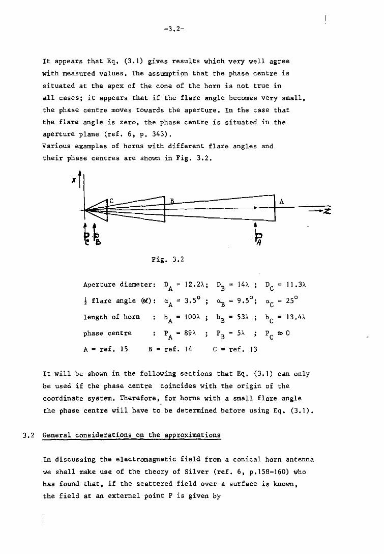
Various examples of horns with different flare angles and

their phase centres are shown in Fig. 3.2.

Fig. 3.2

Aperture diameter: DA = 12.2>.; DB = 14, ; DC

! flare angle (cO: (J.A = 3.50 (J.B = 9.50

; (J.C

length of horn bA = 100, bB = 53, be

phase centre PA = 89, PB = 51. Pc

A = ref. IS B = ref. 14 C = ref. 13

It will be shown in the following sections that Eq. (3. I)

be used if the phase centre coincides with the origin of

= II .3,

= 250

= 13.4,

zO

can only

the

coordinate system. Therefore, for horns with a small flare angle

the phase centre will have to be determined before using Eq. (3.1).

3.2 General considerations on the approximations

In discussing the electromagnetic field from a conical horn antenna

we shall make use of the theory of Silver (ref. 6, p.158-160) who

has found that, if the scattered field over a surface is known,

the field at an external point P is given by

-3.3-

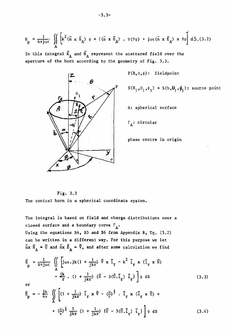
Ep = 4"jWE Jf ~2(n x HA) 1/! + {(n x HA) • 'l('l1/!) + jWE(n x EA) x 'l1/!] dS.(3.2) A

In this integral EA and HA represent the scattered field over the

aperture of the horn according to the geometry of Fig. 3.3.

z. p(R,e,~): fieldpoint

p

A: spherical surface

rA: circular

phase centre in origin

Fig. 3.3

The conical horn in a spherical coordinate system.

The integral is based on field and charge distributions over a

closed surface and a boundary curve rA'

Using the equations B4, BS and B6 from Appendix B, Eq. (3.2)

can be written in a different way. For this purpose we let

nx"HA = U and nx EA m V. and after some calculation we find

E p

or

E P

= 74 .... "..;.j -W':"E

'k m - *

~r ~wE.jk(J + 'kl

) V x I - k2 I x <I xU) I: l: J r r r r A

- ~. (1 + -. -) {U - 3 (U. I ) i} 1/! dS 'k 1 - ] r Jkr r r

ff [(1 1 (1:.) ! (I x U) + "'it) i x V - i x + J r r E r r A

+ (1:.)! 1 (1 1 " {ii - 3(u.I ) I r } ] 1/! dS .....- + "'it) E Jkr J r r

(3.3)

(3.4)

-3.4-

If we make the assumption that

for the second term we find

+ ok) ::::) and use a vector rule J r

or

E = p

E = P

-* \) [ir x V _ (.!:'..) i (Ir·U) i + (.!:'..)! U + E: r s

A

+ (.!:'..)! _01_ {U - 3(u.i ) l')l¢ dS S Jkr r

x V + (.!:'..)! ii () + 0 kl ) S J r

• { 0 (I + J'k3r)}]' I + Jkr

Approximating once more ) I I , finally find + "1t by we

J r

or

E = p

E = p

-* )) [ir A

x V - (.!:'..)! i x (i x u) ] ¢ dS S r r

1 X E - (.!:'..)' A S

Eq. (3.8) is subject to the following restrictions.

). The aperture field is known and spherical and is regarded as

primary source.

2. The currents and fields outside the horn are ignored; this

is better met if the aperture becomes larger in terms of Ao

3. The integration is carried out over an open surface. To

fulfil Maxwell's laws a charge distribution is introduced

along the geometrical optical boundary of the aperture.

In our case the boundary is in the rim of the horn.

4. )+-r--k

1 ~). J r

5. The configuration of the horn behind the aperture (z < b cos a,

Fig. 3.3) is not taken into consideration.

In accordance with these restrictions o may not be too large.

If o is equal to a or smaller, we may expect good results with

Eq. (3.8).

The error made by taking I )

decreases rapidly. +~~1 J r

(3.5)

(3.6)

(3.7)

(3.8)

-3.5-

If, for example, r = SA

I I I I I + 0, 5.10-3 + -:--k :::: J r

arc II + -r.--kl I ~ - 20

J r

3.3 Approximations for well-matched horns

and

If the characteristic wave impedance of the horn is equal or

nearly equal to that of free space in the aperture (120rr ohms),

then

s x E

where s is a unit vector of the Poynting vector S. If the

origin of the coordinate system corresponds with the phase centre,

s = n, therefore,

n.R - n.ii - 0

in the spherical aperture plane of the horn (Fig. 3.3). The components

from Eq. (3.8) can now be simplified since

i x (n x ii ) = <i ii A) n - (n I ) EA ' r A r r

n x HA = n x [~Ii x fA]. (;)i [(Ii fA) n - fA] ~-= - ~ EA,

and _(l:!.) i • ir x [ir x· {-(£)i E } J = <i EA) i - E

E ~ A r r A

Substituting the expressions (3. II) in Eq. (3.8) this becomes

(3.9)

(3. 10)

(3.11)

=* §~A I ) ] -jkr E (J + n - (E I ) (n + I) e • dS , (3.12) p r A r r r

A

which is used by several investigators (reh.14, 15). If a conical

horn is used, the aperture field is assumed to be spherical. In that

case the integral can be solved by substituting in Eq. (3.12) the

following relations:

-3.6-

211 "

s = ) ) b2

sin 0 J d0 J d~ J

o 0

r =

cos y= n.RJ = sin 0 • sin 01

cos (~ - ~I) + cos 0 cos 01

= ;cR:...::c~o~s-!.y_-_b::. r

(see also Fig. 3.3)

For most practical cases the contribution of (EA. ir) (n + ir)

from Eg. (3.12) can be neglected with regard to the contribution

of EA (J

distance

+ n.i ). This seems rather unlikely for cases where the r

from the fieldpoint P to the aperture is smaller than

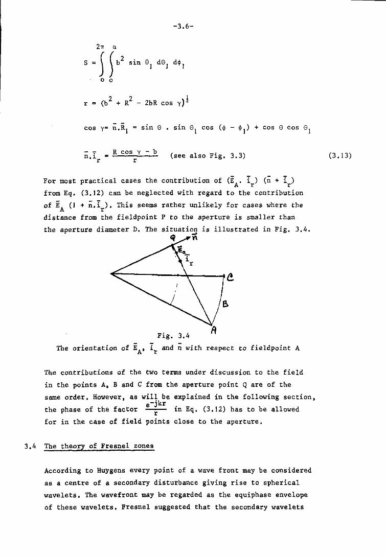
the aperture diameter D. The is illustrated in Fig. 3.4.

Fig. 3.4 A The orientation of EA, ir and n with respect to fieldpoint A

The contributions of the two terms under discussion to the field

in the points A, Band C from the aperture point Q are of the

same order. However, as will be explained in the following section, e-jkr

the phase of the factor r in Eq. (3.12) has to be allowed

for in the case of field points close to the aperture.

3.4 The theory of Fresnel zones

According to Huygens every point of a wave front may be considered

as a centre of a secondary disturbance giving rise to spherical

wavelets. The wavefront may be regarded as the equiphase envelope

of these wavelets. Fresnel suggested that the secondary wavelets

(3.13)

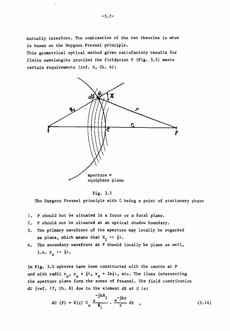
-3.7-

mutually interfere. The combination of the two theories is what

is known as the Huygens Fresnel principle.

This geometrical optical method gives satisfactory results for

finite wavelengths provided the fieldpoint P (Fig. 3.5) meets

certain requirements (ref. 6, Ch. 4):

f

'aperture = equiphase plane

Fig. 3.5

r.: p

The Huygens Fresnel principle with C being a point of stationary phase

I. P should bot be situated in a focus or a focal plane.

2. P should not be situated at an optical shadow boundary.

3. The primary wavefront of the aperture may locally be regarded

as plane, which means that RI » IA. 4. The secondary wavefront at P should locally be plane as well,

i.e. ro » !A,

In Fig. 3.5' spheres have been constructed with the centre at P

and with radii r ,r + o 0

the aperture plane form

dU (ref. 17, Ch. 8) due

lA, r + 2x!A, etc. The lines intersecting o

the zones of Fresnel. The field contribution

to the element dS at Q is:

-jkr dU (P) = K(X) U

o

-jkR I e .;:;,e __ dS

r (3. 14)

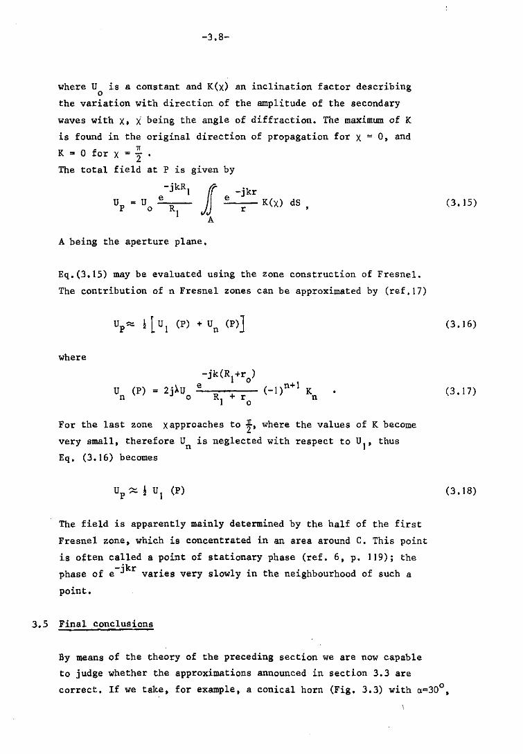
-3.8-

where U is a constant and K(X) an inclination factor describing o

the variation with direction of the amplitude of the secondary

waves with x. X being the angle of diffraction. The maximum of K

is found in the original direction of propagation for X = 0, and 1T

K = 0 for X = 2 . The total field at P is given by

J -jkr U _e_

r- K(X) dS ,

A

A being the aperture plane.

Eq.(3.15) may be evaluated using the zone construction of Fresnel.

The contribution of n Fresnel zones can be approximated by (ref.17)

where

For the last zone xapproaches to t, where the values of K become

very small, therefore Un is neglected with respect to UI

, thus

Eq. (3.16) becomes

The field is apparently mainly determined by the half of the first

Fresnel zone. which is concentrated in an area around C. This point

is often

phase of

point.

called a point of -jkr . e var~es very

3.5 Final conclusions

stationary phase (ref. 6, p. 119); the

slowly in the neighbourhood of such a

By means of the theory of the preceding section we are now capable

(3.15)

(3.16)

(3. 17)

(3. 18)

to judge whether the approximations announced in section 3.3 are

correct. If we take. for example. a conical horn (Fig. 3.3) with a=30o ,

-3.9-

r = b = 12!- (meaning that D = 12!- and kb = 75), and if we take o

the fieldpoint under discussion at a distance R = 22!- from the

aperture, we have an average horn, and are able to compare our

results with those of Li and Turrin (ref. 13).

In the point of stationary phase C (Fig. 3.5) we find that

and

EA' ir = E n A' o

since EA is a tangent to the aperture and EA In. In the vicinity of C also

1 (EA·I ) . (0 + I)I « IEA(l + o.I )1, r r r

We will now prove that the contribution of the entire aperture field

to E is mainly determined by the stationary points C so that p - - --

in Eq. (3.12) (EA.i ) (n+i ) can be neglected with respect to' r r

EA·(I + o.Ir )·

We will assume that the fields in the aperture are equal to the

TEll mode of a circular waveguide with spherical wavefronts.

According to Section 2.8 these fields are given by

and

E = jw~ p

J, (K j I . p) sin m¢

p

, The amplitude over the aperture varies slowly wit~ °1, J

I (x)

. I J ( ) S1n x be1ng of the form cos x and - I x of the form • In the x x H plane for °

1 a a the amplitUde becomes zero. The direction

of polarisation is mainly in the y direction for those parts

of the aperture where EA is largest.

(3. 19)

(3.20)

(3.21)

(3.22)

(3.23)

\/\,~,..,

, " "

--

" "

- -

" " "

--IS'

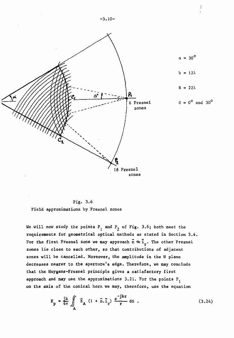
Fig. 3.6

-3.10-

--- ~ .- ~.

6 Fresnel zones

18 Fresnel zones

Field approximations by Fresnel zones

(l =

b = 12A

R = 22A

We will now study the points PI and P2 of Fig. 3.6; both meet the

requirements for geometrical optical methods as stated in Section 3.4.

For the first Fresnel zone we may approach n ~ I . The other Fresnel r

zones lie close to each other, so that contributions of adjacent

zones will be cancelled. Moreover, the amplitude in the H plane

decreases nearer to the aperture's edge. Therefore, we may conclude

that the Huygens-Fresnel principle gives a satisfactory first

approach and may use the approximations 3.21. For the points PI

on the axis of the conical horn we may, therefore, use the equation

-jkr n.I ) ..;;.e __ dS • r r (3.24)

-3.11-

The fieldpoints Pz are chosen in such a way that e ~ a but e < a,

which means.that Pz also meets the requirements of section 3.4.

Therefore, the assumptions made for PI also apply to PZ' The

approximations for Pz are less correct than those for PI as the

adjacent Fresnel zones for Pz points are not symmetrical.

It is also found from a point of view of geometrical optics

that propagation is strongest in the n direction and zero

when perpendicular to n, so that the area around the stationary

points is most important.

Therefore, and keeping in mind the approximations of Sec. 3.4,

for all points P where e < a it is permissible to use Eq.(3.Z0).

Apparently this equation when used for the entire aperture gives

similar results in Case that integration is only carried out over

half the first Fresnel zone.

Measurements have been carried out by Li and Turrin (ref. 13)

and it is noticed that the results correspond very reasonably

with the theory.

-4.1-

4. Literatuur

1. Harrington R.F.:

"Time harmonic electromagnetic fields",

McGraw-Hill Book Company, New York, 1961.

2. Barrow W.L. and Chu L.J.:

"Theory of the electromagnetic horn",

Proc. IRE, pp. 51-64, Jan. 1939.

3. Schorr M.G. and Beck F.J.:

Electromagnetic field of the conical horn",

Journal of applied Physics, vol. 21, pp. 795-801, Aug. 1950.

4. Bucholtz H.:

"Die Bewegung elektromagnetischer wellen in einem Kegelformigen Horn",

Annalen der Physik, Band 37, pp. 173-225, Febr. 1940.

5. Abramowitz M.A. and Stegun J.A.:

"Handbook of mathematical functions",

Dover Publications, New York, 1965.

6. Silver S.:

"Microwave antenna theory and design",

McGraw-Hill Book Company, New York, 1949.

7. Geyer H.:

"Runder Hornstrahler mit ringformigen Sperrtopfen zur gleichzeitigen

Uebertragung zweier polarisationskoppelt;er wellen".

Frequenz, Bd. 20, nr. I, pp. 22-28, Jan. 1966.

8. Lamont H.RtL.:

"Waveguides" ,

Methuen monographs on physical subjects,

London, 1949.

9. watson G.N.:

"A treatise on the theory of Besselfunctions".

Cambridge University Press, Cambridge, 1958.

-4.2-

10. Whittaker E.T. and Watson G.N.:

"A course of modern analysis",

Cambridge University Press, Cambridge, J952.

11. Jones D.S.:

"The theory of electromagnetism",

Pergamon Press Ltd., Oxford, 1964.

12. P iefke G.:

"Reflection at incidence of an Hmn wave at junction of circular

waveguide and conical horn",

Electromagnetic theory and antennas, pp. 209-234,

Pergamon Press, Oxford, 1963.

13. Tingye Li and Turrin R.H.:

"Near-Zone field of the conical horn",

IEEE Transactions on Antennas and Propagation, pp. 800-802, Nov. 1964.

14. Zucker H., Ierley W.H.:

"Computer aided analysis of Cassegrain antennas",

Bell System Techn. Journal, pp. 897-932, July-Aug. 1968.

15. Cook J. S'J Elam E .M. and Zucker H. :

"The open Cassegrain antenna",

Bell System Technical Journal, pp. 1255-1300, Sept. 1965.

16. Schelkunoff S.A.:

"On diffraction and radiation of electromagnetic waves",

Physical Review, pp. 308-3J6, Aug. 1939.

17. Born M. and Wolf E.:

"Principles of Optics",

Pergamon Press, Oxford, 1964.

18. BodmerM.H.:

"Private Communication", 1969.

19. Koop H.E.M.:

Report Graduate Work, T.H. Eindhoven, January 1969.

-AI-

APPENDIX A

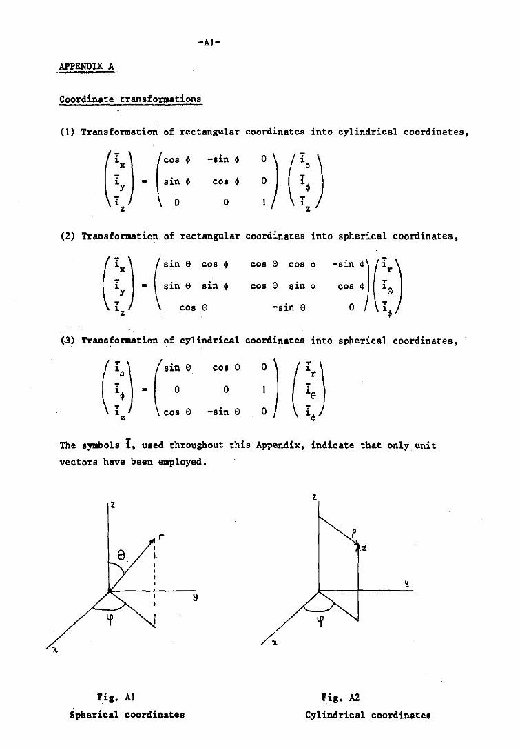
Coordinate transformations

(I) Transformation of rectangular coordinates into cylindrical coordinates,

:: ) c· 4> -sin 4>

:) n: ) - 4> 4> Sl.n cos

0 0 z z

(2) Transformation of rectangular coordinates into spherical coordinates,

U: ) C' cos 4> cos 6 cos 4>

-.in 'W') sin 6 sin <I> 6 sin <I> - cos cos 4> l.6

cos 6 -sin 6 o i4> l.z

(3) Transformation of cylindrical coordinates into spherical coordinates,

n:) sin 6 cos 6

- 0 0

cos 6 -sin 6

o

o z

The symbols i, used throughout this Appendix, indicate that only unit

vectors have been employed.

z

,. e I

I

ria. AI

Spherical coordinates

Fig.A2

Cylindrical coordinates

-BI-

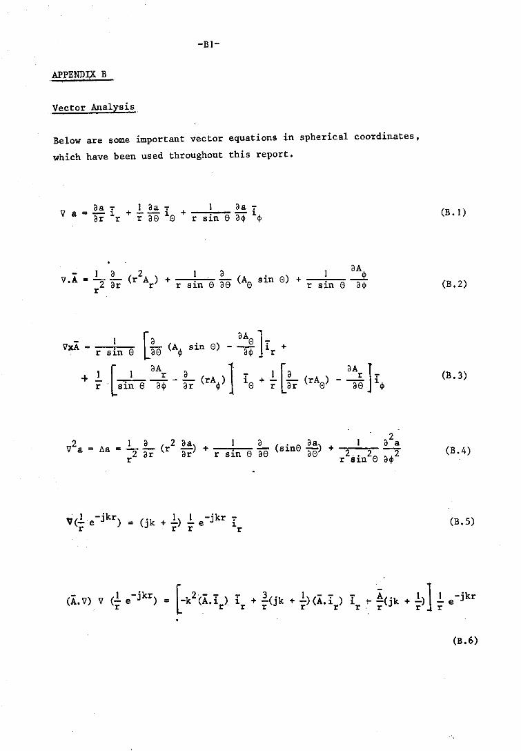
APPENDIX B

Vector Analysis.

Below are some important vector equations in spherical coordinates,

which have been used throughout this report.

V aa.,. + I aa .,. aa .,.

am-1 --1. + -l. a r r r a 88 r sin 8 a $ $

- I a Z a a A", V.A = - - (r A ) + (A sin 8) + ---;...~ -..:t.

rZ ar r r sin 8 ae 8 r sin 8 a$

VZa = 'a I a (rZ aa) a ( aa il = -Z -a a + r s1'n - sin8 -) + r r r 8 as a8

(jk + 1) 1 e-jkr i r r r

-1' 3 ( 'k I) - - - A +-J +-(A.i) i ,...-(jk r r r r r· r

(B. I)

(B. Z)

(B.3)

(B.4)

(B.S)

(B.6)

·-CI-

APPENDIX C

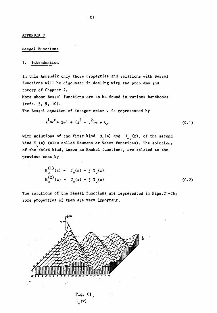
Bessel Functions

I. Introduction

In this Appendix only those properties and relations with Bessel

functions will be discussed in dealing with the problems and

theory of Chapter 2.

More about Bessel functions are to be found in various handbooks

(refs. 5, " 10).

The Bessel equation of integer order v is represented by

1 " 2 2 Z . 'oil + 2w I + (z - v ) w • 0,

with solutions of the first kind jv(z) and J (z), of the second -v kind Y (z) (also called Neumann or Weber functions). The solutions

v of the third kind, known as Hankel functions, are related to the

previous ones by

H~I)(z) - Jv(z) + j Yv(z)

H~2)(z) - Jv(z) - j Yv(z)

The solutions of the Bessel functions are represented in Figs.CI-C6;

some properties of them are very important •

. .. ~ ..

(C.I)

(C.2)

. 1

.1

• . 1

-.1

-.' -.' -.1

-C2-

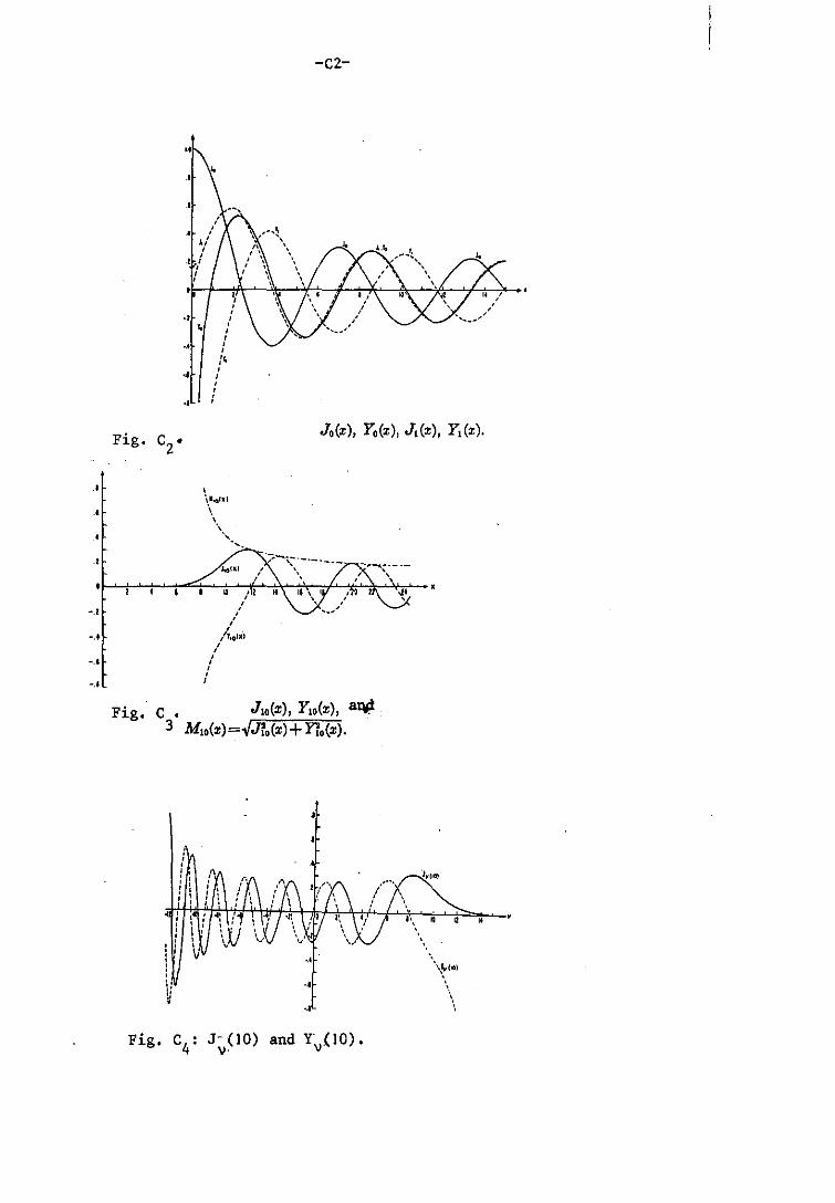
J.(x), 1'.(x), J,(x), 1',(x) .

Fig. C • 3

J IO(x), 1' .. (X), anp M,.(x) =..JJI. (x) + 1'1,(x). .

, "

: , , '" : , \~,!OO)

I! ., ~ \ ••

Fig. C4: J-(10) V·

and Y~(lO) •

-C3-

\I ~ s r7 " , -< e-X "\ .- -

i-!. , 7 7 \ / \, "- /'

0 .... / I\. >< r-... ~

V IX ./ I\. 1/ \. /' ~ / \ / \ / II \ / I\. v' k'

0

II j .\< f..I / 1\ } x 1\ 17 , '\ I'\. / I-... 7- -

• 7 7 ~ IS( ~ i7' \..,/ I'-. f-- V I"-~ ~

I- '-' 1-, , I , , , 7 17 17 "!Iv (vi

-Q .s I II L.-.~~ rJ

/ 7 , 77 7

" IT 7 17 If

-1, 0

,s s r 8 , 10 IJ a -1

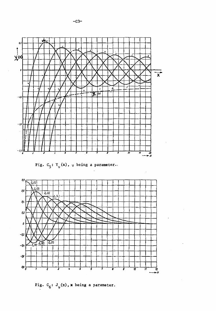
• 1 I • Fig. Cs : Yv(x), v being a parameter"

0. 8 f':" 3,(1)

J,(2)

P\' f'\ 3,(J) , j r\f> ~4) 0.6

1/ f\ '). 1'v '" V' "" " r-, I IJ , ~ I'x '" " 1-... :---rx ''\ [7 , 17 I'" I"'- r-.. J'.. f'

0,2

o f\ '\ r7 " Q j)( +-. t--- t--- f'-.. l- f' l"-

) V\ 7 17 J rt 1\' '\ [7 !\ 17' [7 K 17 -0.2

• kZ':;;t5) .1,(6) J,(7) -0.

2 J , 6 1 B 9 10 11 12 -v

Fig. C6 : Jv(x) , x being a parameter.

-C4-

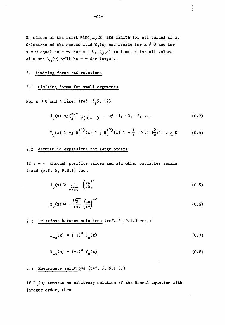
Solutions of the first kind J~(X) are finite- for all values of x.

Solutions of the second kind Y\I (x) are finite for x " 0

x = 0 equal to - ~. For \J .::.. O. J" (x) is limited for all

of x and Y,,(x) will be - ~ for large \J.

2. Limiting forms and relations

2.1 Limiting forms for small arguments

For x ... o and v fixed (ref. 5) 9.1.7)

V-F -1, -2, -3, ...

'V j H(2)(x) \J

1 'V-_

11

2.2 Asymptotic expansions for large orders

and for

values

If v ... ~ through positive values and all other variables remain

fixed (ref. 5, 9.3.1) then

J (x) ~ _1_ (~)V v /211V 2v

Y (x) "" _ \ f2 (ex)-V v ViiV 2v

2.3 Relations between solutions (ref. 5, 9.1.5 etc.)

J (x). (_l)n J (x) -n n

n Y (x) Q (-1) Y (x) -n n

2.4 Recurrence relations (ref. 5, 9.1.27)

If B\J(x) denotes an arbitrary solution of the Bessel equation with

integer order, then

(C.3)

(C.4)

(C.5)

(C.6)

(C.7)

(C.8)

-C5-

~ B (x) a B (X) + BV+I (X) X V v-I

B' (X) = B I(x) - ~ B (x) V v- X V

2.5 Generating functions (ref. 5. 9.1.44. etc.)

'" k cos (x cos ,) = Jo (x) + 2 E (-I) J2k

(x) cos (2k,) k=1

sin (x cos <1» '" k = 2 E (-I) J

2k+

1 (X) cos {(2k + I) IH

k=v

2.6 Asymptotic expansions for large arguments (ref. 5, 9.2.1)

I£v is

where a

function

if

We write

fixed and x'" '" then

Jv(x) =\jk (x -2v + I

11) O(.!.) cos 4 + x

y (x) =~ sin (x - 2v + I 11) + O(.!.)

V 4 x

(I) =~ [j (x -

2v + 11) J + o (!:i) H (x) e X p

V 1IX 4 x

H(2) (x) a ,/2 e x p [_j (x _ 2v + I 11)1 + O(.!.=.i) V V-;x 4 J. x

. '" serl.es E

f(x), k-O ~ x-k is said to be an asymptotic expansion of a

f(x) n-I

- E k-O

-k -n ~ x = O(x ) if x ... .,.

(C.9)

(C.IO)

(C.ll)

(C.12)

(C.13)

(C.14)

(C.15)

(C.16)

(C.17)

(C.18)

(C.19)

(C.20)

-C6-

The series itself may either-be convergent-or divergent (ref. 5, 3.6.15).

2.7 Zeros [Ref. 5, 9.5.12]

If v remains fixed and s » v, the sth zero-point of the Bessel

solutions £Vi S of Jv(x)

The zero-points £' of v,s

and a' of Y'(x) are (s + !v - l)~ vs J'(x) and a of Y (x) are

v 'V,s v

(s + !v - 1) ~

The first positive zero-point in these solutions will be found

for s=I, with the exception that the first zero-point £0,1 of

J~(x) will be zero.

The expansions give a very good approximation also for small

values s > V·

This feature is a well-known property of asymptotic expansions.

3. Bessel functions of fractional order

3.1 Introduction

The Bessel differential equation

z2w" + 2zw' + [z2 - n(n+I)] w = 0

where n=O, ±I, ±2, .•• ,

has particular solutions, namely spherical Bessel functions of the

first kind:

j (z) _ \ r;r n V"2z

of the second kind

y (z) - 'fu Yn+! (z)

and of the third kind

h (I) (z) - j (z) + jYn(z) n n

(C.22)

(C.23)

(C.24)

(C.25)

(C.26)

~·n tal

,

Z

0 I' .

I I i -,' I I ' I ! I I I

-" I

I I I I ,I

I I , -,' I I

jn(lt)

J •••

• • I \~ .

I \ .S I ~ .. nat , ' \ \

f / \,-';,.,.15 ,21 i /\\\ I. \ \ , I I \' \

I I I \ \ I • I \ \ \

-C7-

, / I "\

~~'~'~~~~L-~~~r-~~~-f,bf~T.I-'1 0,", 2 4' 14 I

-,'

-,S

,'0

,0'

,IS I 0 , -.05

-.10

-.1'

-.10

\1 '0 .. •• ___ V

-C8-

or for arbitrary solutions (See also Figs. C7 - C9)

B I (z) V+2

3.2 Limiting values as x + 0 (ref. 5, 10.1.4)

j n (x) -. xn • 71-• ..,3;--"""<5......;'---~~~ } ..... (2n +1)

Yn (X)4 n!1 [I 3 5 •••••• (2n -I~ x

y (-x) -. (_I)n+1 j (x) n -I-n ; n=O.:l,:2,

(ref. 5, 10.1.15).

3.3 Recurrent relations (ref. 5, 10.1.19).

2v + x b (x) = b I (x) + b I (x) v v- v+

(2v+l)b~(x) = vbv

_ 1 (x) - (v+l)bv

+ 1 (x)

b '() b () v + I bv

(x) v x = v_I x - x

3 • 4 ~Th:;;e::...:f;.;;u;;:;;n.;;.c t:;.;i:..:o""n...;h ~,""2 )...;(o.;:x ... )

Following Eq. (C.27) we may write

h (2) (x) v ~. H(2) ( )

- - 1 x. 2x V+2

With Eq. (C.18) we obtain for large x

f

(C.27)

n = 0, 1, 2, '"

(C.28)

... (C.29)

(C.30)

(C.31)

(C.32)

(C.33)

(C.34)

(C.35)

-C9-

For large values of v we find, using the'Eqs';> (C.23, C.24, C.25) and

Eqs. (C.5 and C.6)

h (Z) (x) =\{f [Jv+! (x) 'y (X)J ,;, v - J v+ I

~I& 1 ' ex \1+\ 2' (2V +

1 \1+\ • {(zv + I) ) } ZX Y2'IT (v + !)

or

h,~2) (x) ~ -:-:==1=== [( ex • VZx(2v + 1)' Zv +

+ J ex

+ Z. (Zv + J ex

To obtain a better insight into the function h~Z)(x) we will

first study the behaviour of the function H(Z)\(x). To this end \1+

we write

where M ! = IH(2) (x) I and e ! = Arg H 1 (x) • v+ v+ I v+ v+ 2

According to Abramowitz (ref. 5, 9.2.28) we find for v = constant and

large x:

2 4v - 1

(ZX)Z + ..... J

and 4v2 _

'IT + ..:.:.....,8;-x~ + •••• I

Eqs. (C.38) and (C.39) yield

M IJf2" r 1 + v+ 2 ~iiX

v(v + 1)

zi + ..... ]

\I(v + I) 'IT + 2x

\

I

It is a well-known property of asymptotic expansions that the

function is very well approximated for large values of x. By the

first term of the expansion we may, therefore, conclude that for x > v

(C.36)

(C.37)

(C.38)

(C. 39)

(C .40)

(C.41)

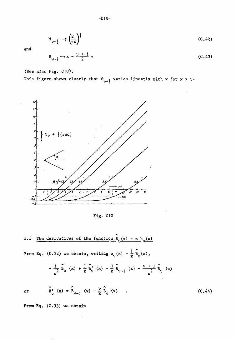
-CIO-

and v + e ~x - 2 11 v+!

(See also Fig. CIO).

This figure shows clearly that Gv+! varies linearly with x for x > v'

12

" 10

9

8

7 t 9 v + !(rad)

5

5

~ " 3

Z

, 0

-f -'!1

-z

Fig. CIO

~

3.5 The derivatives of the function B (x) = x b (x) v v-

I -From Eq. (C.32) we obtain, writing bv(x) = x Bv(x) ,

or

I ~ - - B (x) 2 v x

+ ! if (x) = ! i x v x v-I

.... .... \) ,.. B~ (x) ~ BV_I (x) - x Bv (x)

From Eq. (C.33) we obtain

(x) - v + I -2 Bv

x (x)

(C.42)

(C.43)

(C.44)

-CII-

B' (x) s V + I . B v x v (x) - Bv+ J (x)

Eq. (C.44) now yields

B" (x) a [Bv_1 (x) - ~ B v =-=-ax x v

= B' (x) + ~ B (x).:'" ~ B' (x) v-I 2 ~ . x v x

Substituting Eqs. C44 and C45 in Eq. C46 we obtain

Hence,

= B v

(x) ( -I

.2... [x bv (x)] ax2

3.6 The function

h(2)'(x) I v - + -.:...,.,,.......-x h(2)(x)

v

Using Eq. (C.2?) we find for the derivative of the Hankel function

of the third kind

~ (2)' (x) c ~ [ I rrr . H (2) (x) ] v ax V 2X v+!

I ~ (2) ~ c - - -. H 1 (x) + -2x 2x v+~ 2x (2) ,

Hv+! (x).

As

h~2) (x) .. VI-x H~~~ (x) it is readily seen that

(C.45)

(C.45)

(C.46)

(C.47)

(C.48)

h(2)' (x) v

-C12-

H(2)' (x) 1 + "v+1

- -!it ~x) v+!

h(2)'(x) H(2)'(x) 1 v 1 v+1 it + -h""(2~)-(-X-) = -2x + H(2) (x)

v v+1

or

In accordance with Abramowitz (ref. 5, 9.2.18) we will write

, where

v is a constant and N real. Far large x we obtain the asymptotic

expansions (ref. 5, 9.2.30).

and

N v+1

\ f2 T . v (v + 1) '" ViiX L 1 - 1 2

x

v v2 + v + I ~v+1 '" x - 2 n + 2x + •••••

If x > v Eqs. (C.50) and (c.51) rapidly become

~ N "- -v+1 nx

v ~v+i r... x - 2 n

Using the results found for Hv+1 (x) (Eqs. (C.40) and (C.41) ), it

is readily seen that

'" -j

Therefore, if x» and x > v

(2) , h

1+" ';:;;J' it h (2) -

v

(C.49)

(C.50)

(C.5])

(C. 52)

(C .53)

(C. 54)

(C.55)

2

-e13-

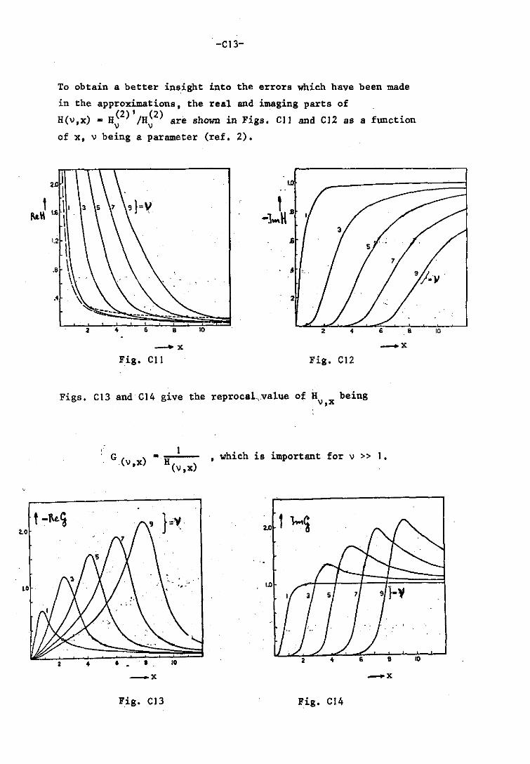
To obtain a better insight into the errors which h'ave been made

in the approximations, the real and imaging parts of

H(v,x) - H~2)'/H~2) are shown in Figs. ell and el2 as a function

of x, v being a parameter (ref. 2).

I LO

I t II t \ 1

1'-&1\ 1:6 \ '

-J ... " 1.2

.8

••

\ .6

I \ & \. ~

'1 2 ~

-x _x

Fig. ell Fig. el2

Figs. el3 and el4 give the reprocal,value of H being v,x

G ( ) - H ' which is important for v » I • . V,x (v,x)

, '.

-x -x

Fig. el3 Fig. el4

-Dl-

APPENDIX D

Legendre functions

I. Introduction

In this Appendix we shall mention some important properties of

Legendre functions as far as they are required to understand

Chapter 2 of the present report. Further properties of Legendre

functions are found in various handbooks and in some papers

(refs. 5, 10 ••••• ).

We will employ Legendre functions only with real arguments x

which are found for z ~ x + j.O.

The associated Legendre equation is

(I - x2) w" - 2xw' + [ v(v

2 +1) - )l 2 J w = 0

I - x

where x = cos e is the argument and e likewise a real number;

v is the degree and )l the order of the equation, and if )l = 0

the equation is called Legendre equation.

The equation has solutions of the first kind p)l (x) and of the v

second kind Q)l (x). We shall only discuss here solutions of the v

first kind.

If V is the non-negative integer n, p~ is called a polynomial n

of degree n, unless )l is a non-negative integer m. In this case

pm is a polynomial of degree n-m, which vanishes identically n

if m> n. The functions in which maO are known as Legendre

polynomials and written P (ref. II, p.79). n

2. Some properties and equations of Legendre functions

If )l - m (m - integer) and x • cos e, the solution of the first

kind (ref. 4) can be written

(D. I)

r(l+v+m) I-x -::~"-'--=--..;..;=--- . F (m-v, m+v+ I; m+ I; 2) 2~()+v-m). r( l+m)

(D.2)

-D2-

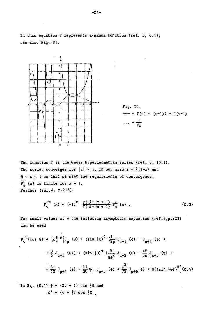
In this equation r represents a-gamma function (ref. 5, 6.1);

see also Fig·. DI.

y

, /

4 / V • V \

• \ / ......

-4

1 .... r-- '"

IV' , , '. " ....... , .. .... .. .. -I .... -0 1 • • 4 !

, Fig. DI.

: "\ " - = r (x) = (x-I)! = II (x-I)

-. =-fx -.

(1

-,

The function F is the Gauss hypergeometric series (ref. 5, 15.1).

The series converges for Izl < I. In our case z = !(I-x) and

e < x < I s6 that we meet the requirements of convergence.

pm (x) is finite for x = I. V

Further (ref.4, p.218).

P -In (x) = (_ I) m r ( II - m + I) pill ( ) v r(t}+m+ J) v x •

For small values of v the following asymptotic expansion (ref.4,p.223)

can be used

+ 16 J\I+3 (ljI)} + (sin Ie) 4 {J!..,.. J 8lj1" \1+2

(D.3)

II 2 . 6J (ljI) - 30 ~. J\I+5 (ljI) + ~ J\I+6 ljI} + O{(sin Ie)} (D.4)

In Eq. (D.4) ljI z (2v + I) sin !e and

ljI' - (v + i) cos je •

-D3-

It is further assumed that 9 + 0; Ivl + ~; x is finite and + 0;

~ and argument v are arbitrary.

Jones (ref. II, p.79) has shown that Eq. (D.4) can be simplified

considerably to

-~ Pv (cos e) = (ljI') J ~

(ljI) [ I + 0(sin2 Ie) 1

The derivative of Eq. (D.S) gives

d -II 'dePv (cos e)

-~ , = - sin e p (cos e) v

If ~ is the non-negative integer m we find from Eqs. (D.S) and (D.6)

m Pv (cos e)

and

IJ

12

11

10

, 6

, G

J

= {-(v+!) cos !e}m. J {(2v +1) m

!... pm (cos e) de v

m' = - sin e • Pv (cos e)

'" '" 1M \

,\ , ' , , \\ 100 \ \.

IQ \'\.

" " ..

fO I

• s ,

z

\ \ '\ \ \. "-\ '\ 'J , , " \. "', ........

''\ '-..{' ....... .. " ........... .. ' .... 4 ......... ..

....... .. ' .... -----

~.-

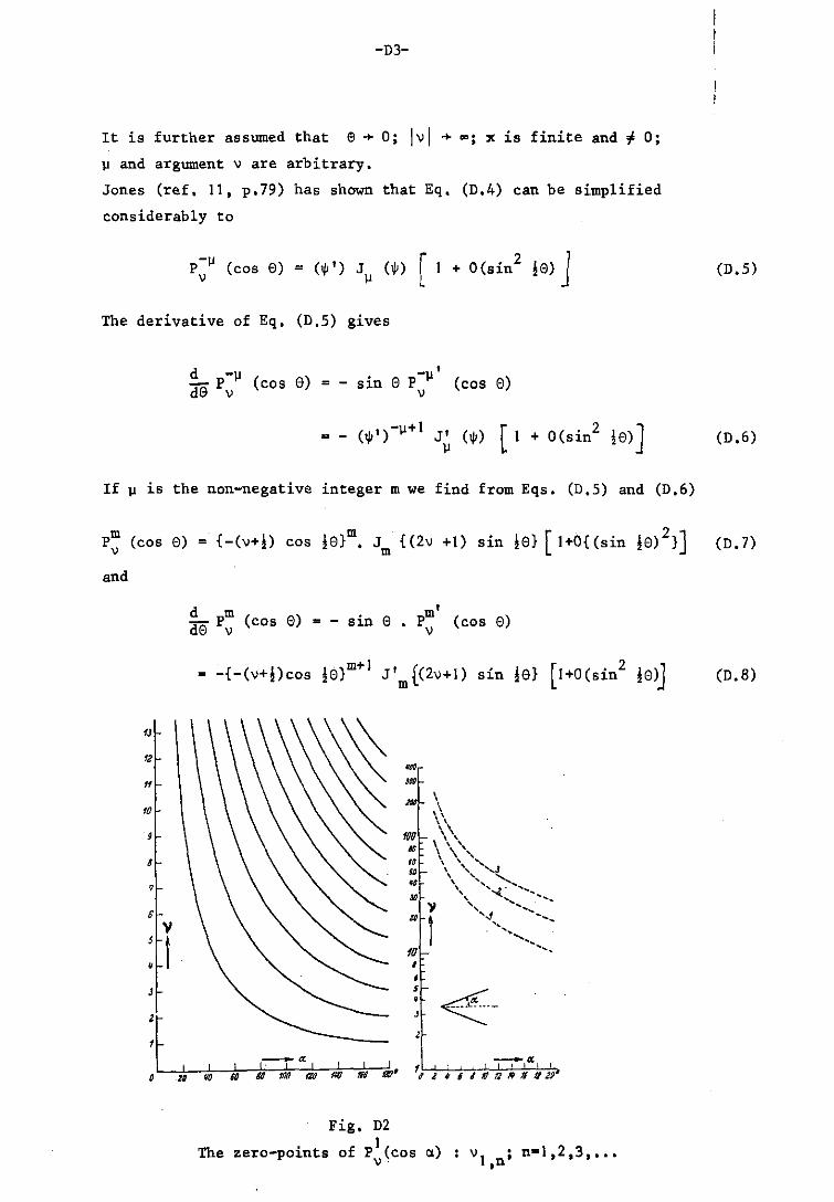
Fig. D2 I The zero-points of P (cos ~) v- VI ;n-l,2,3, ... ,n

(D.S)

(D .6)

(D.7)

(D.B)

-D4-

Eqs. (D.7) and (D.S) hold for small e and large v. These requirements

are met in Chapter 2 as for cones with small e = a, v automatically max

becomes large (Eqs. (2.94) and (2.95) ). The zero-points of the function p~1 (cos a) are graphically given

in Fig. D2, in accordance with Bucholtz (ref. 4). From Eq. (D.3) it

can be seen that these zero-points are equivalent for pI (cos a). v

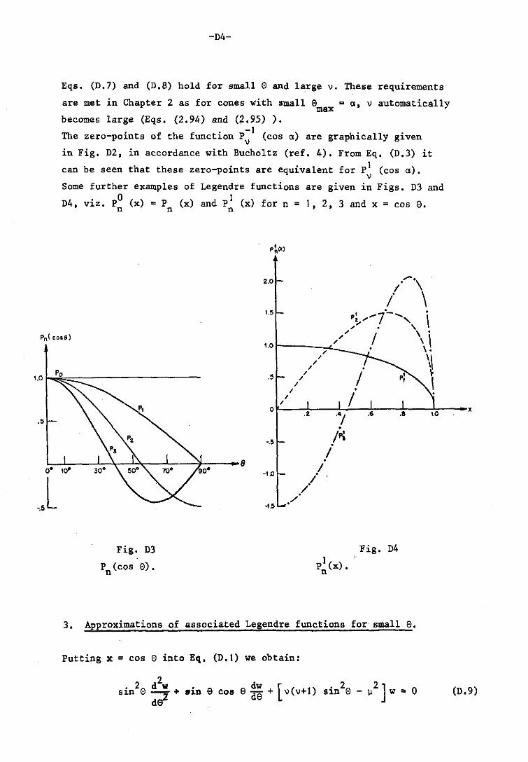
Some further examples of o D4, viz. P (x) = P (x) n n

Legendre functions are given in Figs. D3 and I

and P (x) for n = I, 2, 3 and x = cos 8. n

P~~)

2.0 ....... \ / \

I.. p~'''''7·-'''' . \ " . ,

" / \ Pn( coS9) " , \ "

.. 0 Po

.5

_.,L

Fig. D3

Pn (cos e).

9

'.0

.5

0

-.5

-LO

~~

I I

I I

. /

" " " " " "

.2 .4/ .6 .8

. /p;

.I /

i /" .

Fig. D4 I

Pn

(x).

3. Approximations of associated Legendre functions for small e.

Putting x = cos e into Eq. (D.I) we obtain:

2 . 2 d w • e e dw [( I)

S1.n e ;;:I + 111.0 cos de + v v+

\ . \\ ~

I 1.0

x

(D.9)

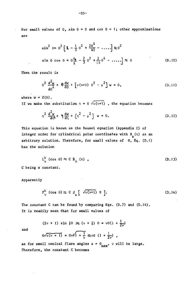
-DS-

For small values of e, sin e ~ e and cos e ~ 1; other approximations

are

.2 2[ 12 S1n e~ e 1 - 3 e

Then the result is

where w ~ f(e).

If we make the substitution n ~ e I~) , the equation becomes

" dw + L- 2 I dn . n

2 jI ] w ~ O.

This equation is known as the Bessel equation (Appendix C) of

integer order for cylindrical polar coordinates with B (n) as an jI arbitrary solution. Therefore, for small values of e, Eq. (D.I)

has the solution

L~ (cos e) "'" C BjI (n) ,

C being a constant.

Apparently

P~ (cos e) ~ C JjI L 1'1('1+1) e 1;

The constant C can be found by comparing Eqs. (D.7) and (D.14).

It is readily seen that for small values of

(2'1 + 1) sin !e :;::: (v + !> e ~ ve(J + ~) and

e/v (v + 1) ~ evvr:-r ~ve (I + -21

) v v

as for small conical flare angles a = e ,v will be large. max Therefore, the constant C becomes

(D. 10)

(D. 11)

(D.12)

(D.13)

(D. 14)

3~--------.--------.--------- 3~~-------,--------,--------,

2~----~~~~-----+--------~

1 1 "\:

"\: ~

a e ___ a 31f 5a"

\; " (J _

-'1 2. 6 -, '\

-1. -1 4 Jl-~

~.5~ J' 3 1

1Pt-- ~ -2 -2

-3L-________ -L ________ -L ______ ~~

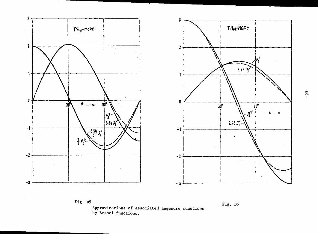
Fig. D5

Approximations of associated Legendre functions by Bessel functions.

Fig. D6

I t:!

'" I

-D7-

c = [-(V + !r +1

The equations (D.7) and (D.14) become equivalent, apart from

a coefficient.

It has been suggested that the above approximations only hold

for small values of e. It appears, however, that associated

Legendre functions can be approximated by Bessel functions

even for large values since e = t ~ (ref. 12). Piefke has

calculated that the error even for values of !IT is smaller than

1%. The Figs. DS and D6 demonstrate the comparison between

Legendre and Bessel functions for TEI2 and TMII modes. For the

TEll mode the difference between the Legendre functions and

the Bessel functions is less than 1% even for e = 1 ~. For other modes it appears that up to a horn aperture angle

of 1200 the mean deviations of the Bessel function from the

Legendre function as referred in the maximum is less than 2%.

The relative errors introduced by Eqs. (D.IO) and (D.II) can,

however, become much larger.

(D.IS)