Embed Size (px)
Citation preview

Analysis and Design of Conical Spiral
Antennas in Free Space and over Ground
A Thesis
Presented to
The Academic Faculty
by
Thorsten W. Hertel
In Partial Fulfillment
of the Requirements for the Degree of
Doctor of Philosophy in Electrical and Computer Engineering
Georgia Institute of Technology
November 2001
Analysis and Design of Conical Spiral Antennas in
Free Space and over Ground
Approved:
Glenn S. Smith, Chairman
Waymond R. Scott, Jr.
Andrew F. Peterson
John A. Buck
Karsten Schwan
Date Approved
ii

ACKNOWLEDGMENTS
This dissertation is the result of my graduate studies at the Georgia Institute of
Technology. Obviously, this work would not have been accomplished without the
support of many people; I would like to express my gratitude to those who have
contributed to this work in one way or another.
Dr. Glenn S. Smith deserves my deepest gratitude for reaching this goal. His
immense knowledge and uncompromising quest for excellence provided an optimum
working environment at Georgia Tech. Dr. Smith has been instrumental in ensuring
my academic and professional well-being over the last five years.
Also, I would like to thank the members of my dissertation committee, Dr.
Waymond Scott, Jr., Dr. Andrew F. Peterson, Dr. John A. Buck, and Dr. Karsten
Schwan. Especially, I would like to express my gratitude to Dr. Scott for giving useful
advice for the measurements and for his courtesy of letting us use his measurement
equipment and the Beowulf Cluster to perform important computer simulations.
In addition, I would like to thank Dr. James G. Maloney and the Georgia Tech
Research Institute for letting us use their calibration kit. Throughout my first few
years at Georgia Tech, Dr. Maloney provided insightful comments on my work.
The discussions and cooperations with all of my colleagues have contributed
substantially to this work: L.E. Rickard Petersson was very helpful in backing up
theoretical issues of my work and Benny Venkatesan assembled and maintained the
Beowulf Cluster and was of valuable help in computer related issues. In particular,
I am very grateful to Dr. Christoph T. Schroder who has been a long-time friend
during college, both in Braunschweig, Germany, and in Atlanta, USA. His academic
iii

ACKNOWLEDGMENTS
excellence and his way of life have always been a great source of motivation.
I am very grateful to many of my friends for their assistance, support, and
extracurricular activities: Dr. Sumeer K. Bhola, Dr. Fabian E. Bustamante, Pawan
Hegde, Holger Junker, Tony V. Mule, Dr. Christoph T. Schroder, Aparna Pappu,
Benny Venkatesan, and Ram Voorakaranam. In particular, I owe special gratitude to
Fabian for many hours of mind-opening discussions and for his culinary treats.
Finally, I would like thank my parents, Jurgen and Elke Hertel, and my brother,
Arne Hertel, for their continuous and unconditional support of all my undertakings,
scholastic and otherwise.
This work was supported in part by the Army Research Office under Contract
DAAG55-98-1-0403.
iv

Contents
ACKNOWLEDGMENTS ii
LIST OF TABLES viii
LIST OF FIGURES ix
SUMMARY xvii
1 Introduction 1
1.1 Historical Overview . . . . . . . . . . . . . . . . . . . . . . . . . . . . 1
1.2 Contribution of Research . . . . . . . . . . . . . . . . . . . . . . . . . 5
1.3 Outline . . . . . . . . . . . . . . . . . . . . . . . . . . . . . . . . . . 8
2 The Two-Arm Conical Spiral Antenna in Free Space 10
2.1 Description of the CSA . . . . . . . . . . . . . . . . . . . . . . . . . . 10
2.2 Characteristics of the CSA in Free Space . . . . . . . . . . . . . . . . 16
3 Parametric Study and Design Graphs 29
4 Resistive Terminations for the CSA 42
4.1 Methods for Terminating the CSA . . . . . . . . . . . . . . . . . . . 42
4.2 Characteristics of the Loaded CSAs . . . . . . . . . . . . . . . . . . . 44
5 The Two-Arm Conical Spiral Antenna over the Ground 57
5.1 General Characteristics of the CSA over the Ground . . . . . . . . . 58
v

CONTENTS
5.2 Numerical Analysis of the CSA over the Ground . . . . . . . . . . . . 66
5.3 GPR Applications . . . . . . . . . . . . . . . . . . . . . . . . . . . . 75
5.3.1 GPR: Detection of Buried Rods . . . . . . . . . . . . . . . . . . 76
5.3.2 GPR: Detection of Buried Mines . . . . . . . . . . . . . . . . . 82
5.4 Removing the Dispersion in the CSA . . . . . . . . . . . . . . . . . . 86
6 FDTD Analysis 98
6.1 FDTD Update Equations . . . . . . . . . . . . . . . . . . . . . . . . 99
6.1.1 Update Equations in Continuous Space . . . . . . . . . . . . . . 100
6.1.2 Update Equations in Discretized Space . . . . . . . . . . . . . . 105
6.1.3 Medium Properties in the FDTD Update Equations . . . . . . . 110
6.1.4 FDTD Update Equations for the Resistive Elements . . . . . . . 115
6.1.5 FDTD Update Equations for a Dipole . . . . . . . . . . . . . . 117
6.2 Validation of PML . . . . . . . . . . . . . . . . . . . . . . . . . . . . 121
6.3 FDTD Modeling of the CSA . . . . . . . . . . . . . . . . . . . . . . . 122
6.4 FDTD Antenna Feed . . . . . . . . . . . . . . . . . . . . . . . . . . . 125
6.5 Near-Field to Far-Field Transformer . . . . . . . . . . . . . . . . . . 132
6.6 Program/Code Parallelization . . . . . . . . . . . . . . . . . . . . . . 133
7 Validation of FDTD Results 138
7.1 Validation using Published Results . . . . . . . . . . . . . . . . . . . 138
7.1.1 CSA in Free Space . . . . . . . . . . . . . . . . . . . . . . . . . 138
7.1.2 Horizontal Dipole over Lossy Media . . . . . . . . . . . . . . . . 142
7.2 Validation using Georgia Tech Measurements . . . . . . . . . . . . . 144
7.2.1 Manufacturing of the CSA . . . . . . . . . . . . . . . . . . . . . 145
7.2.2 Feed System of the CSA . . . . . . . . . . . . . . . . . . . . . . 149
7.2.3 Termination of the CSA . . . . . . . . . . . . . . . . . . . . . . 155
7.2.4 Impedance Measurements . . . . . . . . . . . . . . . . . . . . . 159
7.2.5 Realized Gain Measurements . . . . . . . . . . . . . . . . . . . . 165
7.2.6 Dipole Measurements . . . . . . . . . . . . . . . . . . . . . . . . 169
vi

CONTENTS
8 Conclusions 175
APPENDIX A Analysis of the Resistive Sheet Termination 178
APPENDIX B Convergence Study for FDTD Feed Models for An-
tennas 183
BIBLIOGRAPHY 197
VITA 201
vii

List of Tables
3.1 Hybrid bandwidth results as a function of D/d for a CSA with a)θ = 15, α = 80, δ = 90, b) θ = 7.5, α = 75, δ = 90, and c)θ = 5, α = 60, δ = 90. . . . . . . . . . . . . . . . . . . . . . . . . . 40
5.1 Electrical parameters for different soil conditions at f = 1.8GHz. . . 63
6.1 Short-hand notation and staggered positions in time and space for allelectric and magnetic fields within the Yee cell (i, j, k). . . . . . . . . 107
6.2 Averaging of the electrical properties in the FDTD update equations. 1126.3 Electrical parameters for different soil conditions at f = 0.7GHz. . . 1226.4 Relative errors for the electric field at various observation points in the
grid for three different soil conditions. . . . . . . . . . . . . . . . . . . 1236.5 Normalization of the parameters in the transmission-line equations. . 128
B.1 Parameters of the discretized linear dipole antenna of square crosssection. . . . . . . . . . . . . . . . . . . . . . . . . . . . . . . . . . . . 187
B.2 Ratio of numerical phase velocity to the speed of light for differentdiscretizations. . . . . . . . . . . . . . . . . . . . . . . . . . . . . . . 188
B.3 Resonant frequencies and the conductances at anti-resonance for thehard source (best case for convergence). . . . . . . . . . . . . . . . . . 196
viii

List of Figures
1.1 Geometry for the practical two-arm CSA (top) and side view of thebasic cone (bottom). . . . . . . . . . . . . . . . . . . . . . . . . . . . 3
1.2 Schematic drawings for two models of the CSA: a) using thin wires, b)antenna arms with expanding arm width. . . . . . . . . . . . . . . . . 4
1.3 a) “Infinite balun” introduced by Dyson [9], b) balun and impedancetransformer introduced by Wills [16]. . . . . . . . . . . . . . . . . . . 6
1.4 The two-arm CSA placed in air directly over the ground. . . . . . . . 7
2.1 a) Geometry for the practical two-arm CSA, b) side view of the basiccone, and c) top view of the highlighted planar cut. . . . . . . . . . . 11
2.2 a) Schematic model for the a) left-handed CSA and b) right-handedCSA. . . . . . . . . . . . . . . . . . . . . . . . . . . . . . . . . . . . . 14
2.3 a) Schematic drawing for pulses of charge at three instances of time(top view of CSA), b) polarization ellipse for the electric field for anobserver beyond the small end looking in the direction of the negative zaxis, c) polarization ellipse for the electric field for an observer beyondthe large end looking in the direction of the positive z axis, and d)illustration for the position and orientation of the observers. . . . . . 15
2.4 a) Differentiated Gaussian pulse as a function of normalized time, t/τp,b) spectrum of the differentiated Gaussian pulse as a function of nor-malized frequency, ωτp, and c) far-zone electric field on axis. . . . . . 17
2.5 Theoretical results for the reflected voltage at the terminals of theunloaded CSA. . . . . . . . . . . . . . . . . . . . . . . . . . . . . . . 18
2.6 Comparison of theoretical (FDTD) and measured terminal quantities:a) magnitude of the reflection coefficient, b) input resistance, and c)input reactance for the unloaded CSA with θ = 7.5, α = 75, δ = 90,D/d = 8 (d = 1.9 cm). . . . . . . . . . . . . . . . . . . . . . . . . . . 19
2.7 Theoretical results for the input impedance plotted on a Smith chartfor a) 0.3GHz ≤ f ≤ 3.5GHz and b) 0.5GHz ≤ f ≤ 3.5GHz . . . . . 21
2.8 Comparison of theoretical (FDTD) and measured input reactances. Asmall capacitance, C = 0.12 pF, has been added in parallel with theterminals. . . . . . . . . . . . . . . . . . . . . . . . . . . . . . . . . . 22
ix
LIST OF FIGURES
2.9 Theoretical results for the far-zone pattern for the right-handed andleft-handed circularly polarized components of the electric field at thefrequencies: a) f = 0.75GHz, b) f = 1.50GHz, and c) f = 2.25GHz. 23
2.10 Theoretical results for the front-to-back ratio referred to a) the to-tal far-zone electric field and b) the left-handed circularly polarizedcomponent of the far-zone electric field. . . . . . . . . . . . . . . . . . 25
2.11 a) Schematic drawing for the polarization ellipse, b) theoretical resultsfor the axial ratio for the electric field in the far zone of the CSA. . . 26
2.12 a) Theoretical and measured results for the realized gain and b) the-oretical results for the gain. The results are for the direction of maxi-mum radiation (−z). . . . . . . . . . . . . . . . . . . . . . . . . . . . 28
3.1 Frequencies that define various bandwidths: a) the bandwidth forVSWR, b) the bandwidth for directivity, and c) the hybrid bandwidth. 30
3.2 Design graphs for the unloaded CSA based on the results for the VSWR(Zc = R∞) showing a) the bandwidth, b) the maximum wavelength,λmax, and c) the minimum wavelength, λmin, as functions of the anglesθ and α, with δ = 90. . . . . . . . . . . . . . . . . . . . . . . . . . . 32
3.3 Design graphs for the unloaded CSA based on the results for the direc-tivity showing a) the hybrid bandwidth, b) the maximum wavelength,λmax, and c) the minimum wavelength, λmin, as functions of the anglesθ and α, with δ = 90. . . . . . . . . . . . . . . . . . . . . . . . . . . 33
3.4 Design graphs for the unloaded CSA showing a) the hybrid bandwidth,b) the maximum wavelength, λmax, and c) the minimum wavelength,λmin, as functions of the angles θ and α, with δ = 90. . . . . . . . . 34
3.5 Design graph for the unloaded CSA showing the average input impedanceof the infinitely-long CSA as a function of the angles θ and α, withδ = 90. . . . . . . . . . . . . . . . . . . . . . . . . . . . . . . . . . . 35
3.6 Design graphs for the unloaded CSA showing a) the average directivity,b) the average half-power beamwidth, and c) the average front-to-backratio as functions of angles θ and α, with δ = 90. . . . . . . . . . . 37
3.7 Design graph for the CSA showing the average axial ratio as a functionof the angles θ and α, with δ = 90. . . . . . . . . . . . . . . . . . . 38
3.8 Theoretical results for the VSWR (a,c,e) and the directivity (b,d,f)as a function of frequency with D/d as parameter. The results arefor a CSA with a) and b) θ = 15, α = 80, δ = 90, c) and d)θ = 7.5, α = 75, δ = 90, and e) and f) θ = 5, α = 60, δ = 90. . . 39
4.1 a) The loaded CSA including the feed system, b) simple transmission-line model. . . . . . . . . . . . . . . . . . . . . . . . . . . . . . . . . . 43
4.2 Schematic drawings for the two resistive terminations: a) two lumpedresistors connecting the ends of the spiral arms, b) a resistive sheetcovering the entire end of the cone. . . . . . . . . . . . . . . . . . . . 44
x

LIST OF FIGURES
4.3 a) Theoretical results for the reflected voltage at the terminals of theantenna that contains only the reflection from the drive point, b) the-oretical results for the input impedance of the infinitely long CSA. . . 46
4.4 Theoretical results for the reflected voltage at the terminals of theantenna for the unloaded CSA (solid line), the CSA terminated withlumped resistors (dashed line), and the CSA terminated with a resistivesheet (dash-dotted line). . . . . . . . . . . . . . . . . . . . . . . . . . 47
4.5 Theoretical results for the CSA with and without the resistive termina-tions: a) the magnitude of the reflection coefficient, b) input resistance,and c) input reactance. . . . . . . . . . . . . . . . . . . . . . . . . . . 48
4.6 Smith charts for a) the unloaded CSA, b) the CSA terminated withlumped resistors, and c) the CSA terminated with a resistive sheet. . 49
4.7 Theoretical results for the CSA terminated with the lumped resistors:the far-zone patterns for the right-handed and left-handed circularlypolarized components of the electric field at the frequencies: a) f =0.75GHz, b) f = 1.50GHz, and c) f = 2.25GHz. . . . . . . . . . . . 50
4.8 Theoretical results for the CSA terminated with a resistive sheet: thefar-zone patterns for the right-handed and left-handed circularly po-larized components of the electric field at the frequencies: a) f =0.75GHz, b) f = 1.50GHz, and c) f = 2.25GHz. . . . . . . . . . . . 51
4.9 Theoretical results for a) the front-to-back ratio referred to the totalfar-zone electric field, b) front-to-back ratio referred to the left-handedcircularly polarized component of the far-zone electric field, and c)axial ratio for the total far-zone electric field. . . . . . . . . . . . . . . 53
4.10 a) Schematic drawing for determining the dissipated power for theCSA terminated with lumped resistors (left) and the CSA terminatedwith a resistive sheet (right). Theoretical results for the b) dissipatedpower and c) efficiency for the CSA terminated with lumped resistors(solid) and for the CSA terminated with a resistive sheet (dashed). . 54
4.11 Theoretical results for the a) realized gain, b) gain, and c) directivityin the direction of maximum radiation (−z). . . . . . . . . . . . . . . 56
5.1 CSA over the ground with the virtual apex of the antenna placed atthe air/ground interface. . . . . . . . . . . . . . . . . . . . . . . . . . 58
5.2 Schematic drawing to illustrate the scaling of the electric field of theCSA in the ground. . . . . . . . . . . . . . . . . . . . . . . . . . . . . 60
5.3 Schematic drawings of the polarization ellipses for the electric field:for transmission, maximum reception, and null reception. The ellipsesin a) are for the most general case (elliptical polarization) and in b)for the special case of circular polarization; c) position and orientationof the observers. . . . . . . . . . . . . . . . . . . . . . . . . . . . . . . 62
5.4 Idealized polarization characteristics of the left-handed CSA for trans-mission and reception. . . . . . . . . . . . . . . . . . . . . . . . . . . 63
xi
LIST OF FIGURES
5.5 a) Geometry of the plane-wave analysis. Analytical results for themagnitude of the reflection coefficient for the electric field b) parallelto the plane of incidence and c) perpendicular to the plane of incidence. 64
5.6 Analytical results for the ratio |ErefLHCP/E
refRHCP|2 as a function of angle
of incidence αinc for three different types of soil. Polarization ellipsesfor the incident and reflected electric fields are shown for the medium-moist soil. . . . . . . . . . . . . . . . . . . . . . . . . . . . . . . . . . 66
5.7 Schematic drawing to illustrate that the use of circular polarizationreduces the effect of the air/ground interface on the antenna response. 67
5.8 Comparison of the input impedances for the CSA in free space andover medium-moist soil. . . . . . . . . . . . . . . . . . . . . . . . . . 68
5.9 Theoretical results for a) the reflected voltage of the CSA over groundand b) the voltage of the signal scattered from the air/ground interface. 69
5.10 a) Theoretical results for the normalized electric field on axis as afunction of depth: in free space (solid line), in the lossy, medium-moistsoil (dashed line), and in the lossless medium-moist soil (dash-dottedline). b) Theoretical results for the axial ratio on axis for the CSA infree space at the apex (solid line), for the CSA over the medium-moistsoil observed 4 cm (dashed line), and 1m (dash-dotted line) below theair/ground interface. . . . . . . . . . . . . . . . . . . . . . . . . . . . 71
5.11 a) The normalized electric field distribution 4 cm below the air/groundinterface as a function of frequency and distance from the axis. b)Results for the normalized 3 dB width as a function of frequency forthe antenna in free space observed at the apex (solid line) and for theantenna over the medium-moist ground observed at 4 cm below theapex (dashed line). . . . . . . . . . . . . . . . . . . . . . . . . . . . . 73
5.12 The axial ratio at a depth of 4 cm below the air/ground interface as afunction of frequency and distance from the axis. . . . . . . . . . . . 74
5.13 Theoretical results for a) the electric field of the CSA in free space inthe near field of the antenna and b) the electric field scattered fromthe air/ground interface. . . . . . . . . . . . . . . . . . . . . . . . . . 75
5.14 Schematic drawing for a monostatic GPR that uses a single CSA todetect thin metallic rods buried in the ground. . . . . . . . . . . . . . 76
5.15 Illustration for the detection approach using a CSA in a monostaticGPR. . . . . . . . . . . . . . . . . . . . . . . . . . . . . . . . . . . . . 77
5.16 Drawing detailing the parametric study for four differently sized rodsburied in the ground using a) a single CSA and b) four resonant dipolesas the GPR antennas. . . . . . . . . . . . . . . . . . . . . . . . . . . 79
5.17 Theoretical results for the parametric study for a) the monostatic GPRusing a single CSA and b) a series of resonant dipoles to detect thinmetallic rods buried in the ground. . . . . . . . . . . . . . . . . . . . 80
5.18 Theoretical results for the electric field scattered from the rod buriedin the ground. . . . . . . . . . . . . . . . . . . . . . . . . . . . . . . . 81
xii
LIST OF FIGURES
5.19 Results for the monostatic GPR with the thin rods buried in the drysoil. . . . . . . . . . . . . . . . . . . . . . . . . . . . . . . . . . . . . 82
5.20 a) Schematic drawing for the monostatic GPR used to detect buriedplastic mines, b) parameters that describe the mine and the relativepositioning of the antenna and the mine. . . . . . . . . . . . . . . . . 83
5.21 Theoretical results for the parametric study for the monostatic GPRusing a single CSA to detect buried plastic mines: a) DM = 18 cm, b)DM = 13.5 cm, and c) DM = 9 cm. . . . . . . . . . . . . . . . . . . . 85
5.22 Theoretical results for the electric field scattered from the buried mine:a) on axis and b) off axis. . . . . . . . . . . . . . . . . . . . . . . . . 87
5.23 Schematic model for a monostatic radar to detect an infinitely longpipe in free space . . . . . . . . . . . . . . . . . . . . . . . . . . . . . 88
5.24 Theoretical results for the reflected voltage of the CSA a) in free spaceand b) the CSA in free space with the target; c) results for the voltageof the signal scattered from the pipe in free space. . . . . . . . . . . . 90
5.25 Examples for scatterers of co polarization using a) an anisotropic mediumand b) a grid of closely spaced wires. . . . . . . . . . . . . . . . . . . 91
5.26 Theoretical results for the circularly polarized components of the elec-tric field scattered from the grid, normalized by the incident, LHCPcomponent of the electric field. . . . . . . . . . . . . . . . . . . . . . . 92
5.27 Theoretical results for the received voltage of the signal scattered fromthe pipe in free space with the dispersion removed: a) signal in thefrequency domain, b) signal in the time domain for −0.5 ≤ t/τL ≤ 4,and c) signal in the time domain for 0.5 ≤ t/τL ≤ 1.5. . . . . . . . . . 94
5.28 Schematic model for a monostatic radar to detect the infinitely longpipe buried in the ground. . . . . . . . . . . . . . . . . . . . . . . . . 95
5.29 Theoretical results for a) the reflected voltage of the CSA above the dryground with the pipe present and b) the voltage of the signal scatteredfrom the pipe. . . . . . . . . . . . . . . . . . . . . . . . . . . . . . . . 96
5.30 Theoretical results for the received voltage of the signal scattered fromthe pipe buried in dry ground with the dispersion removed: a) is for−0.5 ≤ t/τL ≤ 4, and b) for 0 ≤ t/τL ≤ 1. . . . . . . . . . . . . . . . 97
6.1 Schematic drawing for the open-region problem truncated by the PMLabsorbing boundary condition (CSA is omitted for simplicity). . . . . 101
6.2 Yee cell in three dimensions. . . . . . . . . . . . . . . . . . . . . . . . 1066.3 Details about the correct averaging at an interface of the electrical
properties for a) the electric field Ex and b) the magnetic field Hz. . . 1116.4 a) Spatial variation of the conductivity σx a) along its longitudinal
direction x and b) along its transverse direction z with the air/groundinterface present. . . . . . . . . . . . . . . . . . . . . . . . . . . . . . 113
6.5 Implementing the lumped resistor in the FDTD method. . . . . . . . 115
xiii
LIST OF FIGURES
6.6 Implementing the resistive sheet in the FDTD method: a) the three-dimensional Yee cell containing the resistive sheet and b) slice of theFDTD grid in the vicinity of the sheet. . . . . . . . . . . . . . . . . . 117
6.7 a) Schematic model of the dipole antenna, b) drawing of a Yee cellthat contains the antenna conductor. . . . . . . . . . . . . . . . . . . 118
6.8 Cross-sectional view of a) a single Yee cell that contains the antennaconductor, b) Yee cells in the vicinity of the drive-point gap, and c)Yee cell near the antenna end. . . . . . . . . . . . . . . . . . . . . . . 120
6.9 Schematic drawing for the approach to validate the PML (only theregion surrounding the antenna is shown, the PML is omitted for sim-plicity). . . . . . . . . . . . . . . . . . . . . . . . . . . . . . . . . . . 121
6.10 Schematic drawing detailing the FDTD modeling of the antenna armsin a two-step process. . . . . . . . . . . . . . . . . . . . . . . . . . . . 123
6.11 FDTD model of the conical spiral antenna. Only 10% of the antennaat the feed end is shown. . . . . . . . . . . . . . . . . . . . . . . . . 124
6.12 Discretized version of the feeding disc. . . . . . . . . . . . . . . . . . 1256.13 Schematic model of a) the one-dimensional transmission line and b)
the feed region including the virtual transmission line. . . . . . . . . . 1276.14 Model of the surface used for the near-field to far-field transformation. 1346.15 Division of the solution space into subspaces. . . . . . . . . . . . . . 1356.16 Illustration for the necessary message passing of interface data (fields). 137
7.1 Comparison of theoretical (FDTD) and measured reflection coefficientsplotted on a Smith chart for a) the unloaded CSA and b) the CSAterminated with lumped resistors. The results are for Ramsdale’s CSA[17] with θ = 15, α = 60, δ = 90, and D/d = 12.77 with D = 15.2 cm.140
7.2 Comparison of theoretical (FDTD) and measured far zone patternsfor the circularly polarized components of the electric field for a) theunloaded CSA and b) the CSA terminated with lumped resistors (RL =300Ω) at f = 0.5GHz. The results are for Ramsdale’s CSA [17] withθ = 15, α = 60, δ = 90, and D/d = 12.77 with D = 15.2 cm. . . . . 141
7.3 Schematic model for the horizontal dipole placed over the ground. . . 1427.4 Comparison of the analytical and FDTD proximity losses for the hor-
izontal dipole over the ground. The analytical results are from [48]. . 1437.5 Comparison of the theoretical (FDTD) and measured results for the in-
put admittance of the horizontal dipole antenna over tap water arounda) the first resonance and b) the second resonance. The experimentalresults are from [49]. . . . . . . . . . . . . . . . . . . . . . . . . . . . 144
7.6 Illustration on how the conical surface becomes a circular sector andvice versa. . . . . . . . . . . . . . . . . . . . . . . . . . . . . . . . . . 146
7.7 Schematic drawings for the unwrapped surface of the cone for a) θ ≤14.5 and b) 14.5 < θ ≤ 30. . . . . . . . . . . . . . . . . . . . . . . 147
xiv

LIST OF FIGURES
7.8 a) Template for the copper etching process, b) photograph of the man-ufactured flexible circuit board. . . . . . . . . . . . . . . . . . . . . . 148
7.9 a) Photograph of the planar circuit board before it takes on the shapeof the conical surface, b) photograph of the assembled CSA. . . . . . 150
7.10 Details of the method used to feed the CSAs in the measurements. . 1517.11 a) Photograph of the rigid circuit board used to connect the feed cable
with the antenna arms, b) photograph of the feed region. . . . . . . . 1527.12 Photograph of a) the vector network analyzer and b) the balun used
in the measurement. . . . . . . . . . . . . . . . . . . . . . . . . . . . 1537.13 Schematic drawings for the two-port measurements of the balun: a) is
for determining S11, S12, S21, and S22, b) for S11, S13, S31, and S33, andc) for S22, S23, S32, and S33. . . . . . . . . . . . . . . . . . . . . . . . . 154
7.14 Measured results for the a) insertion loss, b) return loss, and c) phasedifference between the output ports. . . . . . . . . . . . . . . . . . . . 156
7.15 Photograph of a) the lumped resistor termination (chip resistor sol-dered to the wires) and b) the big end of the CSA when terminatedwith lumped resistors. . . . . . . . . . . . . . . . . . . . . . . . . . . 157
7.16 Schematic drawing for the measurement of the lumped resistor. . . . 1577.17 Measured results for the impedance of the lumped resistor with RL =
200Ω. . . . . . . . . . . . . . . . . . . . . . . . . . . . . . . . . . . . 1587.18 Photograph of a) the resistive sheet, modified to properly attach at
the antenna end and b) the big end of the CSA when terminated withthe resistive sheet.. . . . . . . . . . . . . . . . . . . . . . . . . . . . . 159
7.19 a) Schematic model for the resistive sheet used in the measurement,b) comparison of the analytical and experimental results for the DCresistance. . . . . . . . . . . . . . . . . . . . . . . . . . . . . . . . . . 160
7.20 Photograph of the measurement setup to determine the input impedance.1617.21 Comparison of theoretical (FDTD) and measured terminal quantities
for the unloaded antenna: a) magnitude of the reflection coefficient, b)input resistance, and c) input reactance for the CSA with θ = 7.5,α = 75, δ = 90, D/d = 8 (d = 1.9 cm). . . . . . . . . . . . . . . . . 162
7.22 Comparison of theoretical (FDTD) and measured terminal quantitiesfor the antenna terminated with lumped resistors: a) magnitude of thereflection coefficient, b) input resistance, and c) input reactance for theCSA with θ = 7.5, α = 75, δ = 90, D/d = 8 (d = 1.9 cm). . . . . . 163
7.23 Comparison of theoretical (FDTD) and measured terminal quantitiesfor the antenna terminated with a resistive sheet: a) magnitude of thereflection coefficient, b) input resistance, and c) input reactance for theCSA with θ = 7.5, α = 75, δ = 90, D/d = 8 (d = 1.9 cm). . . . . . 164
7.24 Comparison of theoretical (FDTD) and measured input reactances forthe antenna terminated with a resistive sheet. A small capacitance,C = 0.12 pF, has been added in parallel with the terminals. . . . . . . 165
xv

LIST OF FIGURES
7.25 a) Photograph of the measurement setup to determine the realizedgain, b) schematic model for the two-antenna method. . . . . . . . . 166
7.26 Drawing detailing the wavelength-dependent distance R(λ) betweenthe active regions. . . . . . . . . . . . . . . . . . . . . . . . . . . . . . 167
7.27 Comparison of theoretical (FDTD) and measured realized gains (lin-ear) for the CSA with θ = 7.5, α = 75, δ = 90, D/d = 8(d = 1.9 cm): a) the unloaded antenna, b) the antenna terminatedwith lumped resistors, and c) the antenna terminated with a resistivesheet. . . . . . . . . . . . . . . . . . . . . . . . . . . . . . . . . . . . . 168
7.28 Schematic model of the dipole used in the measurement. . . . . . . . 1697.29 Measurement setup for the dipole antenna. . . . . . . . . . . . . . . . 1707.30 Schematic FDTD model of a) the dipole with square cross section
including the details of the feed region and b) the simple straight dipole.1707.31 Comparison of theoretical (FDTD) and measured results for the dipole
with the square cross section including the details of the antenna feed:a) input impedance, b) realized gain, and c) gain. . . . . . . . . . . . 172
7.32 Comparison of theoretical (FDTD) and measured results for the dipolewith the straight cross section omitting the details of the antenna feed:a) input impedance, b) realized gain, and c) gain. . . . . . . . . . . . 174
A.1 Drawing detailing the conformal mappings. . . . . . . . . . . . . . . . 179A.2 Drawing detailing the Schwarz-Christoffel transformation. . . . . . . 181A.3 Normalized DC sheet resistance as a function of the angular electrode
width δ. . . . . . . . . . . . . . . . . . . . . . . . . . . . . . . . . . . 182
B.1 Schematic drawings showing the feed region of the antenna. . . . . . 184B.2 a) Model of the linear dipole with square cross section, b) discretization
of the model (L/w = 30.5). . . . . . . . . . . . . . . . . . . . . . . . . 186B.3 Feeding techniques shown for the first three discretizations (worst case
for convergence). . . . . . . . . . . . . . . . . . . . . . . . . . . . . . 189B.4 Results for the input admittance in the worst case for convergence: a)
hard-source model and b) simple feed. . . . . . . . . . . . . . . . . . 190B.5 Schematic illustration of the change of the susceptance with varying
length of the gap. . . . . . . . . . . . . . . . . . . . . . . . . . . . . . 190B.6 Schematic drawing for the fringing of the electric field in the vicinity
of the drive-point gap. . . . . . . . . . . . . . . . . . . . . . . . . . . 191B.7 Feeding techniques shown for the first three discretizations (best case
for convergence). . . . . . . . . . . . . . . . . . . . . . . . . . . . . . 192B.8 a) Proper scaling of the reference planes in the transmission line, b)
correct virtual connection of the transmission line at the feed point. . 193B.9 Results for the input admittance in the best case for convergence: a)
hard-source model and b) simple feed. . . . . . . . . . . . . . . . . . 194
xvi

LIST OF FIGURES
B.10 Comparison of the results for the admittance: a) worst case and b)best case for convergence. . . . . . . . . . . . . . . . . . . . . . . . . 195
xvii

SUMMARY
In this research, the two-arm, conical spiral antenna (CSA) is investigated for its
use as a transmitting and receiving antenna for all applications in free-space, e.g.,
telecommunications and electromagnetic compatibility and for its use when placed
over the ground, e.g., in a ground-penetrating radar (GPR). This antenna belongs
to the class of frequency-independent antennas, and has uniform performance char-
acteristics, such as input impedance, gain, and circular polarization over a broad
frequency range. These are desirable features for the above applications. The CSA
is analyzed using the finite-difference time-domain (FDTD) numerical method and
validated by comparison with measurements of the input impedance and the realized
gain. A parametric study is performed using the FDTD analysis, and the results
from the study are used to produce new design graphs for this antenna. The graphs
supplement and extend the existing, mainly empirical, design base for this antenna.
Two resistive terminations, intended to improve the low-frequency performance, are
examined. One is a termination formed from two lumped resistors, and the other is
a new termination formed from a thin disc of resistive material. When the CSA is
placed directly over the ground with its axis normal to the surface of the ground, it
may be useful for applications in which signals must be transmitted into the ground
and/or received from within the ground. Qualitative arguments based on the geo-
metrical and electrical properties of the CSA isolated in free space show that the
beneficial properties of the CSA in free space are preserved when placed over the
ground. Results from a complete analysis of the CSA over the ground are used to
quantitatively verify these arguments. Illustrative examples are presented in which
xviii

SUMMARY
the CSA is used in a monostatic GPR.
xix

CHAPTER 1
Introduction
In this work, the two-arm, conical spiral antenna (CSA) is investigated when isolated
in free space, e.g., for its use in telecommunications and electromagnetic compatibility
[1]-[4], and when it is placed over the ground, e.g., for its use in a ground-penetrating
radar (GPR) [5]. This antenna belongs to the class of frequency-independent anten-
nas, i.e., it has uniform performance characteristics, such as input impedance, gain,
and circular polarization over a broad range of frequencies, which makes it beneficial
for the above applications.
1.1 Historical Overview
The genesis of the CSA was in the work of Rumsey during the 1950s [6, 7]. Rumsey
introduced two necessary conditions for practical, frequency-independent antennas of
this type: the angle principle and the truncation principle. Briefly stated, the angle
principle says that the performance of an antenna that is defined entirely by angles
will be frequency independent. Evidently, this implies an infinite antenna geometry
and thus an infinite frequency range of operation, so an additional consideration is
needed for practical antennas. The truncation principle says that the antenna must
have an “active region” of finite size. An active region is that part of the antenna that
contributes the most to the radiation at one frequency. As the frequency is changed,
it moves on the antenna in such a way that the dimensions of this region, expressed
1
1.1 Historical Overview
in terms of wavelength, remain constant; hence, the performance remains constant.
The antenna performance is then practically frequency independent over the range
of frequencies for which the active region is completely contained within the finite
structure of the antenna.
In 1959, Dyson first introduced the equiangular planar spiral antenna as a prac-
tical frequency-independent antenna that is defined mainly by angles [8]. Based on
measurements, he created design curves for some important antenna characteristics,
such as the beamwidth and the axial ratio. The planar spiral antenna radiates equally
in two directions simultaneously, and for many applications an antenna is needed with
a beam in only one direction. The CSA described below satisfies this requirement.
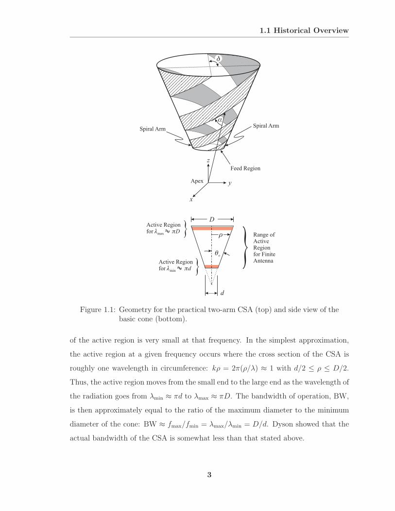
The two-arm CSA that satisfies Rumsey’s principles for practical frequency in-
dependence is shown in Fig. 1.1. Three angles define the geometry of the infinite CSA:
the half angle of the cone θ, the wrap angle α, and the angular width of the antenna
arms δ. The practical CSA is bounded in its minimum and maximum diameters of
the truncated cone, d and D, respectively. The active region, as shown by the gray
areas at both ends of the CSA, moves along the cone towards increasing diameter
with decreasing frequency. Consequently, the highest frequency is radiated from the
small end where the CSA is usually fed and the lowest frequency is radiated from the
large end. Dyson first described this antenna in 1959 [9]-[11], and later in a seminal
paper he provided comprehensive information for its design [12]. This paper contains
an extensive, experimentally based survey of two-arm CSAs. Dyson performed a se-
ries of measurements on these antennas and used these results to construct design
graphs. An important element in this procedure was the measurement of the current
distribution on the arms of the CSA (actually the magnetic field close to the arms).
The current was then used to determine the active region, and the movement in terms
of wavelength of the active region along the arms was used to establish the bandwidth
of operation.
Dyson showed that the active region is that part of the antenna that contributes
the most to the radiation at a particular frequency. This is because the current outside
2
1.1 Historical Overview
r1 r1
o
d
D
x
y
z
Apex
Spiral ArmSpiral Arm
Active Regionfor min d
Active Regionfor max D
Range ofActiveRegionfor FiniteAntenna
Feed Region
Figure 1.1: Geometry for the practical two-arm CSA (top) and side view of thebasic cone (bottom).
of the active region is very small at that frequency. In the simplest approximation,
the active region at a given frequency occurs where the cross section of the CSA is
roughly one wavelength in circumference: kρ = 2π(ρ/λ) ≈ 1 with d/2 ≤ ρ ≤ D/2.
Thus, the active region moves from the small end to the large end as the wavelength of
the radiation goes from λmin ≈ πd to λmax ≈ πD. The bandwidth of operation, BW,
is then approximately equal to the ratio of the maximum diameter to the minimum
diameter of the cone: BW ≈ fmax/fmin = λmax/λmin = D/d. Dyson showed that the
actual bandwidth of the CSA is somewhat less than that stated above.
3

1.1 Historical Overview
(b)(a)
SpiralArm #1
SpiralArm #1
SpiralArm #2
SpiralArm #2
Figure 1.2: Schematic drawings for two models of the CSA: a) using thin wires,b) antenna arms with expanding arm width.
Yeh and Mei [13, 14] applied Hallen’s integral equation to the CSA to solve for
the currents on the antenna arms using the Method of Moments. In their models, the
method is often based on a thin-wire model for the CSA, see Fig. 1.2a, in which the
antenna arms are modeled with an effective wire radius. Since these model does not
scale with operating wavelength, it is not truly frequency independent. For frequency
independence, the arms must expand in width as they move away from the apex of
the cone, as shown in Fig. 1.2b.
In 1977, Miller first investigated CSAs in the time domain with a time-domain
integral equation method [15]. The main objective was to optimize the antenna for
pulsed excitation. Ideally, the incident signal should cover a wide range of frequencies,
but often, the low-frequency content of a pulsed signal causes long settling times of
the antenna response and consequently requires long execution times. Miller studied
various pulse forms that are commonly used in numerical time-domain methods and
that represent a trade-off between broadband incident signals and small settling times.
He proposed the modulated Gaussian pulse; this is a sinusoidal signal modulated with
a Gaussian envelope.
Wills proposed a two-arm CSA for submarine communication [16]. While most
researchers before him investigated the thin-wire model, Fig. 1.2a, he studied the
antenna with thin metallic, expanding antenna arms, Fig. 1.2b, empirically. In the
4
1.2 Contribution of Research
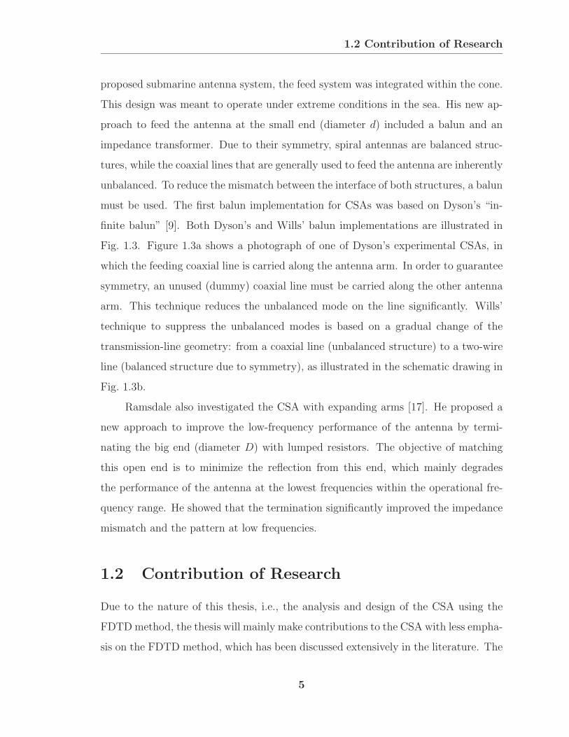
proposed submarine antenna system, the feed system was integrated within the cone.
This design was meant to operate under extreme conditions in the sea. His new ap-
proach to feed the antenna at the small end (diameter d) included a balun and an
impedance transformer. Due to their symmetry, spiral antennas are balanced struc-
tures, while the coaxial lines that are generally used to feed the antenna are inherently
unbalanced. To reduce the mismatch between the interface of both structures, a balun
must be used. The first balun implementation for CSAs was based on Dyson’s “in-
finite balun” [9]. Both Dyson’s and Wills’ balun implementations are illustrated in
Fig. 1.3. Figure 1.3a shows a photograph of one of Dyson’s experimental CSAs, in
which the feeding coaxial line is carried along the antenna arm. In order to guarantee
symmetry, an unused (dummy) coaxial line must be carried along the other antenna
arm. This technique reduces the unbalanced mode on the line significantly. Wills’
technique to suppress the unbalanced modes is based on a gradual change of the
transmission-line geometry: from a coaxial line (unbalanced structure) to a two-wire
line (balanced structure due to symmetry), as illustrated in the schematic drawing in
Fig. 1.3b.
Ramsdale also investigated the CSA with expanding arms [17]. He proposed a
new approach to improve the low-frequency performance of the antenna by termi-
nating the big end (diameter D) with lumped resistors. The objective of matching
this open end is to minimize the reflection from this end, which mainly degrades
the performance of the antenna at the lowest frequencies within the operational fre-
quency range. He showed that the termination significantly improved the impedance
mismatch and the pattern at low frequencies.
1.2 Contribution of Research
Due to the nature of this thesis, i.e., the analysis and design of the CSA using the
FDTDmethod, the thesis will mainly make contributions to the CSA with less empha-
sis on the FDTD method, which has been discussed extensively in the literature. The
5
1.2 Contribution of Research
main contributions of this research are three fold, viz, providing new design graphs
for the CSA, investigating resistive terminations for CSAs, and analyzing CSAs in
free space when placed directly over the ground. In this research, the frequency-
independent model of the CSA, i.e., with expanding arm width, is examined both
numerically and experimentally. To date, only the wire model has been studied
numerically that often does not satisfy the conditions for practical frequency inde-
pendence and that is clearly outperformed by the full model of the CSA (with the
expanding arm width).
(a)
(b)
FeedingCoaxialLine
DummyCoaxialLine
Section ThroughConductors
N-Type 50
Coaxial InputConnector
100 alanced
Line Output
DielectricInnerConductor
OuterConductor
Figure 1.3: a) “Infinite balun” introduced by Dyson [9], b) balun andimpedance transformer introduced by Wills [16].
6

1.2 Contribution of Research
A parametric study for the CSA is performed using the FDTD analysis, and the
results from this study are used to produce new design graphs. These graphs supple-
ment and extend the design information provided by Dyson [12]. The bandwidths for
the impedance and the pattern of the antenna are calculated directly from the results
for these quantities, unlike Dyson’s study, where the bandwidth is inferred from an
examination of the active region for the antenna.
The CSA has desirable features for applications in which antennas are placed
in air over the ground, see Fig. 1.4, and used to transmit signals into the ground or
to receive signals coming from within the ground. Simple physical arguments show
that the frequency-independent performance of the CSA isolated in free space can
be preserved when placed over the ground, and that the use of circular polarization
can minimize the effect of the air/ground interface on the antenna response. Thus,
parameters such as the input impedance should be the same as those when the antenna
is isolated in free space. Using simple scaling, it can be shown that the near field also
exhibits frequency independence. To date, no one has investigated the properties of
this antenna over the ground in such detail. This knowledge about the characteristics
of the CSA over the ground is used to study the CSA in a monostatic GPR.
Earth
Figure 1.4: The two-arm CSA placed in air directly over the ground.
7
1.3 Outline
In earlier work, based on limited experimental results, the resistive termination
at the open end of the antenna was shown to improve the low-frequency performance
for just two properties [17]: the impedance and the pattern. In this thesis, the effect
of two different resistive terminations on the performance of the antenna is examined
in more detail. In the first configuration, lumped resistors are connected in parallel
with the antenna arms. In the second and new configuration, a circular disc cut from
a thin sheet of resistive material connects the two arms.
1.3 Outline
The outline of this thesis is as follows. In Chapter 2, the two-arm CSA is inves-
tigated when isolated in free space. Main performance characteristics such as the
impedance, the gain, and the pattern of this antenna are presented, and the accu-
racy of the FDTD model is verified using measurements of the input impedance and
the realized gain. In Chapter 3, a parametric study is performed using the FDTD
analysis, and the results from this study are used to produce new design graphs for
this antenna. These graphs supplement and extend the empirical results of Dyson.
Two resistive terminations, intended to improve the low-frequency performance of
the CSA, are studied in Chapter 4: lumped resistors connected between the arms at
the open end, and a new configuration, a thin disc of resistive material connected to
the arms at the open end. The effect of the resistive terminations on the performance
of the CSA is examined, and some guidelines are offered for their use. In Chapter
5, qualitative arguments based on the geometrical and electrical properties of the
isolated CSA are used to determine the performance when the CSA is placed over
the ground. Results from a complete analysis of the CSA over the ground, performed
with the FDTD method, are used to quantitatively verify these arguments. Illus-
trative examples are given in which the CSA is used in a monostatic GPR. Chapter
6 is concerned with the finite-difference time-domain (FDTD) method used to ana-
lyze this antenna numerically. The typical FDTD update equations are derived for
8

1.3 Outline
the perfectly matched layer (PML) absorbing boundary condition that truncates the
open region surrounding the antenna and absorbs outgoing electromagnetic energy
with negligible reflection. Other key elements in this analysis are the near-field to
far-field transformer (for the results in free space) to obtain the radiated or far-zone
field of the antenna, and the one-dimensional transmission-line feed to conveniently
study the voltage reflected from the antenna drive point. In order to greatly reduce
the execution time of the simulation, the computer code can be parallelized to run
the simulation on a multiple-processor architecture. In Chapter 7, the FDTD method
is validated with measured results from the published literature and with new mea-
surements performed at Georgia Tech. The published results are for a CSA in free
space both unloaded and loaded (terminated using lumped resistors) and for hori-
zontal dipoles placed directly over the ground. The Georgia Tech measurements are
for a CSA in free space unloaded and loaded (terminated using lumped resistors and
a resistive sheet). For these measurements, two identical CSAs were manufactured
using flexible printed circuit board material with the metallic antenna arms on this
sheet formed by a wet chemical etch. Measured results for the input impedance and
the realized gain are used to validate the FDTD analysis.
There are two appendices to this thesis. In Appendix A, the DC resistance of
the circular resistive sheet measured between circular electrodes of angular width δ is
determined. The solution is accomplished by means of two conformal mappings. In
Appendix B, two common FDTD feed models for antennas are studied for convergence
with increasing discretization. The objective of this convergence study is to provide
guidelines for the proper positioning and scaling of elements in the feed model.
9
CHAPTER 2
The Two-Arm Conical Spiral Antenna in
Free Space
This chapter is concerned with the analysis and design of the two-arm, conical spiral
antenna (CSA) in free space using the finite-difference time-domain (FDTD) method.
First, the antenna geometry and characteristics of the radiated electric field are de-
scribed in Section 2.1. In Section 2.2, several antenna performance characteristics are
presented for one antenna geometry. To validate the numerical analysis, results for
the input impedance and the realized gain are compared with measurements.
2.1 Description of the CSA
The geometry for the two-arm CSA is shown in Fig. 2.1. The antenna is constructed
by winding two metallic strips around the surface of a truncated cone. Three angles
define the geometry of the frequency-independent CSA. These are the half angle of
the cone, θ, the wrap angle, α, and the angular width of the arms, δ. The half angle
of the cone is measured between the symmetry axis and the side of the cone. When
θ = 90, the CSA becomes a planar spiral, which radiates equally in two directions
(±z) [8]. When θ is small, the radiation from the CSA is predominantly along the
axis of the cone in the direction of the apex (−z).1 The rate of wrap of the arms
1The main radiation direction (−z) for the CSA might be unexpected; one might expect the
main beam of the antenna to be end fire, i.e., in the propagation direction of the guided wave that
10

2.1 Description of the CSA
o
d
D
y
x
z
x
y
z
Apex
Arm 2Arm 1
rd
r1 r1
R
(a)
(b) (c)
z
Figure 2.1: a) Geometry for the practical two-arm CSA, b) side view of thebasic cone, and c) top view of the highlighted planar cut.
around the conical surface is defined by the angle α. This is the angle between the
spiral arm and the radial line from the apex of the cone, as shown in Fig. 2.1a. The
third angle, δ, defines the constant angular width of the arms everywhere along the
cone and is illustrated in Fig. 2.1c, which is the top view of the highlighted plane in
Fig. 2.1a. The results in this thesis are limited to the most common configuration,
is launched at the small end and traveling towards the big end (towards +z direction). Dyson
compared the CSA with a bifilar helix and showed using a Brillouin diagram, also referred to as
k−β diagram [18, 19], that the radiation from the CSA is in fact backfire (−z) within the frequency
range of operation [12].
11

2.1 Description of the CSA
δ = 90, which is sometimes referred to as “self-complementary design.” In this case,
the metallic arms are identical in size and shape to the open regions on the conical
surface. Generally, this value gives the most desirable characteristics for radiation.
For this antenna to be practical, it must be of finite size. As shown in Fig. 2.1b,
the extent of the antenna is limited by the minimum and maximum diameters of the
cone, d and D, respectively.
The boundaries of the arms for the two-arm CSA can be described mathemati-
cally with expressions for the radial distance, r, from the apex of the cone to a point
on the conical surface [12]. As illustrated in Fig. 2.1a, r1 describes the distance from
the apex of the cone to one boundary of the first arm, and r1δ describes the distance
from the apex to the other boundary of the same arm, i.e.,
r1(φ) = rd eb|φ|, |φ| ≥ 0 (2.1)
and
r1δ(φ) = rd eb(|φ|−δ), |φ| ≥ δ. (2.2)
Here, b is defined as
b =sin θtanα
, (2.3)
and rd = d/(2 sin θ) is the radial distance from the apex of the cone to the smaller
end of the cone (diameter d). Note that the magnitude of φ is not limited to 2π.
Values of |φ| > 2π are permitted, because the exponential functions in (2.1) and (2.2)
are not periodic. The two arms are symmetric to the z axis (diametrically opposite),
so the boundaries of the second arm can be obtained by rotating the boundaries of
the first arm by the angle π, i.e.,
r2(φ) = rd eb(|φ|−π), |φ| ≥ π (2.4)
and
r2δ(φ) = rd eb(|φ|−π−δ), |φ| ≥ π + δ. (2.5)
Simple geometry can be used to determine other characteristic parameters of the
antenna, that will frequently be used throughout the analysis and the design of CSAs:
12

2.1 Description of the CSA
the height of the cone (measured from the apex of the cone to the big end)
hc =D
2 tan θ, (2.6)
the height of the CSA (measured from the small end to the big end)
hs =D − d
2 tan θ, (2.7)
and the total length of the spiral arms (measured along the surface of the cone)
Ls =D − d
2 sin θ cosα. (2.8)
The radiation from a well-designed CSA is maximum in the direction of the −z
axis, and in this direction, the electric field is predominantly circularly polarized. The
sense of the circular polarization, viz, right-handed or left-handed, is determined by
the direction in which the arms are wound around the cone. For the antenna shown
in Fig. 2.1a, the polarization is left-handed circular, and the antenna is referred to
as a left-handed CSA. There is an easy way to remember the relationship between
the state of polarization for the radiation and the direction of the winding: For an
antenna that radiates left-handed circular polarization, with the thumb of the left
hand pointing in the direction of maximum radiation (−z), the fingers, when curled
to form a fist, point in the direction the arms are traced out in going from the small
end to the large end of the cone,2 see Fig. 2.2a. The radii that describe the antenna
arms of the left-handed CSA (r1, r1δ, r2, and r2δ) are given by (2.1)-(2.5) with φ ≥ 0
and z > 0. As shown in Fig. 2.2b, for a right-handed CSA, the winding sense for the
arms is reversed; therefore, φ ≤ 0 and z > 0.
2Notice that the arms of the left-handed CSA in Fig. 2.1a are traced out with the sense of a
right-handed screw: The arms spiral around the +z axis in clockwise sense as z is increased. So
another way of remembering the relationship between the state of polarization for the radiation and
the direction of the winding is that a left-handed CSA (one that produces a left-handed circularly
polarized field in the direction for maximum radiation) has the arms wound with the sense of a
right-handed screw.
13

2.1 Description of the CSA
(b)(a)
SpiralArm #2
SpiralArm #2
SpiralArm #1
SpiralArm #1
Left-Handed CSA Right-Handed CSA
Figure 2.2: a) Schematic model for the a) left-handed CSA and b) right-handedCSA.
The characteristics of the electric field radiated from a left-handed CSA are
illustrated schematically in Fig. 2.3. Figure 2.3a is the top view looking from the big
end of the CSA down towards the small end. For simplicity, the thin-wire model of
the antenna is used for this simple argument. Since the antenna is fed at the small
end, pulses of charge propagate along each antenna arm towards the open end of the
CSA. Due to the out-of-phase excitation, one antenna arm carries a pulse of positive
charge and the other arm a pulse of negative charge, between which an electric field
can be measured. The positions of the pulses of charge and the corresponding electric
fields are shown for three instances in time, t = t1, t2, and t3, with t1 < t2 < t3. The
circular rotation of the electric field with time is evident and illustrated schematically
using polarization ellipses in Figs. 2.3b and c. Notice that the ellipse in Fig. 2.3b is
traced out counterclockwise for an observer located beyond the small end looking in
the direction of the negative z axis, while the ellipse in Fig. 2.3c is traced out clockwise
for an observer located beyond the big end looking in the direction of the positive z
axis. Both directions are directions of propagation for the corresponding waves. The
positions of the observers and their orientation are illustrated in Fig. 2.3d. Following
the convention used by the IEEE [20], the polarization ellipse in Fig. 2.3b corresponds
to left-handed circular polarization (LHCP), while the polarization ellipse in Fig. 2.3c
corresponds to right-handed circular polarization (RHCP).
14

2.1 Description of the CSA
-
-
-
+
+
+
E( )t2
E( )t1
E( )t3
Pulse ofNegativeCharge
Pulse ofPostitiveCharge
y
ExEx
x
EyEy
z
z-z
RHCPLHCP
(a)
(b) (c)
(d)
AntennaArms
xy
z
Observer (b)
Observer (c)Direction ofPropagation(- )z
Sense ofRotationfor ( )E t
Direction ofPropagation( )z
Figure 2.3: a) Schematic drawing for pulses of charge at three instances oftime (top view of CSA), b) polarization ellipse for the electric fieldfor an observer beyond the small end looking in the direction ofthe negative z axis, c) polarization ellipse for the electric field foran observer beyond the large end looking in the direction of thepositive z axis, and d) illustration for the position and orientationof the observers.
15
2.2 Characteristics of the CSA in Free Space
2.2 Characteristics of the CSA in Free Space
In this section, important antenna parameters are presented to demonstrate the ben-
eficial properties of CSAs, such as uniform impedance, unidirectional radiation, and
circular polarization over a broad range of frequencies. The results presented are for
the left-handed CSA with the following parameters: θ = 7.5, α = 75, δ = 90,
D/d = 8 with d = 1.9 cm, and Zc = 100Ω. A pair of identical CSAs with above pa-
rameters was constructed, and measurements of the input impedance and the realized
gain of these antennas were used to validate the FDTD analysis. The details of the
measurements (construction, feeding, results) will be discussed in detail in Chapter
7, while only some results are presented here.
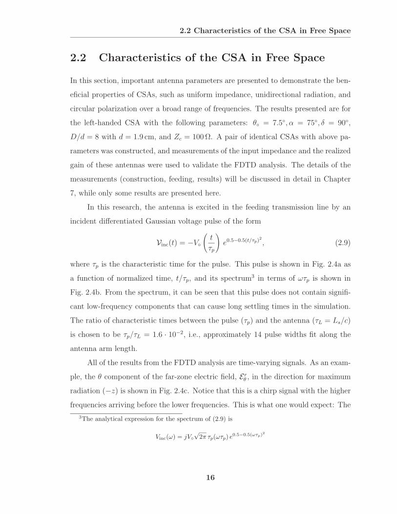
In this research, the antenna is excited in the feeding transmission line by an
incident differentiated Gaussian voltage pulse of the form
Vinc(t) = −V
(t
τp
)e0.5−0.5(t/τp)
2
, (2.9)
where τp is the characteristic time for the pulse. This pulse is shown in Fig. 2.4a as
a function of normalized time, t/τp, and its spectrum3 in terms of ωτp is shown in
Fig. 2.4b. From the spectrum, it can be seen that this pulse does not contain signifi-
cant low-frequency components that can cause long settling times in the simulation.
The ratio of characteristic times between the pulse (τp) and the antenna (τL = Ls/c)
is chosen to be τp/τL = 1.6 · 10−2, i.e., approximately 14 pulse widths fit along theantenna arm length.
All of the results from the FDTD analysis are time-varying signals. As an exam-
ple, the θ component of the far-zone electric field, Erθ , in the direction for maximum
radiation (−z) is shown in Fig. 2.4c. Notice that this is a chirp signal with the higher
frequencies arriving before the lower frequencies. This is what one would expect: The
3The analytical expression for the spectrum of (2.9) is
Vinc(ω) = jV√2π τp(ωτp) e0.5−0.5(ωτp)2
16
2.2 Characteristics of the CSA in Free Space
-4 -2 0 2 4
-1.0
-0.5
0.0
0.5
1.0
t / p
Vin
c(
)/
tV
o
(a)
t / L
0.0 0.5 1.0 1.5 2.0
-1.0
-0.5
0.0
0.5
1.0
E,
no
rm
()t
r
(c)
-4 -2 0 2 4
-1.0
-0.5
0.0
0.5
1.0
p
(b)
j VV
inc(
)/ (
)
o
Figure 2.4: a) Differentiated Gaussian pulse as a function of normalized time,t/τp, b) spectrum of the differentiated Gaussian pulse as a functionof normalized frequency, ωτp, and c) far-zone electric field on axis.
higher frequencies are radiated near the small end of the cone so they travel a shorter
distance to reach the far zone than the lower frequencies that are radiated near the
large end of the cone. The frequency-domain results for the CSA are obtained by
Fourier transforming signals such as those shown in Fig. 2.4a and c.
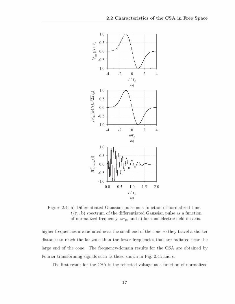
The first result for the CSA is the reflected voltage as a function of normalized
17

2.2 Characteristics of the CSA in Free Space
-1 0 1 2 3 4 5 6
-0.2
-0.1
0.0
0.1
0.2
0.3
t / L
Vre
fo
/V
Drive PointReflection
Second EndReflection
First EndReflection
Figure 2.5: Theoretical results for the reflected voltage at the terminals of theunloaded CSA.
time, t/τL, see Fig. 2.5. The reflection at t/τL ≈ 0 is caused by the drive point, i.e.,
the interface between the feeding transmission line and the antenna terminals. A
pulse with an amplitude of roughly 80% of the incident pulse is transmitted through
this interface. The reflection from the antenna end enters the antenna response at
integer multiples of the round-trip time along the antenna arms, i.e., multiples of 2τL.
Notice that the two end reflections are small and thus suggest that most of the signal
is radiated by the CSA.
In Fig. 2.6, the FDTD results (solid line) and measured results (dashed line)
for the magnitude of the reflection coefficient and the input impedance (resistance
and reactance) of the CSA with θ = 7.5, α = 75, δ = 90, D/d = 8 (d =
1.9 cm) are graphed as a function of frequency (logarithmic scale). The resistance
is about 150Ω and the reactance is small over a large range of frequencies, i.e.,
0.5GHz ≤ f ≤ 3.5GHz.4 Notice that the FDTD results match the measured results
“ripple for ripple,” although there is some offset of the two curves, which will be
discussed later. At frequencies below 0.5GHz, the large oscillations in the resistance
4Most frequency domain results in this section are presented over the frequency range 0.3GHz ≤f ≤ 3.5GHz. For comparison, the range determined from the active region, in its simplest approxi-mation, extends from fmin = c/(πD) = 0.6GHz to fmax = c/(πd) = 5.0GHz.
18
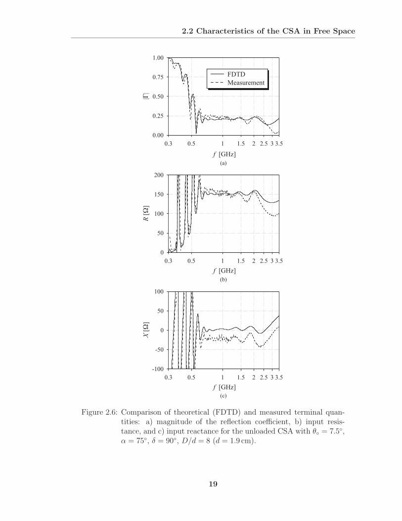
2.2 Characteristics of the CSA in Free Space
0.3 0.5 1 1.5 2 2.5 3 3.5
0.00
0.25
0.50
0.75
1.00
f [GHz]
||
0.3 0.5 1 1.5 2 2.5 3 3.5
0
50
100
150
200
f [GHz]
R[
]
0.3 0.5 1 1.5 2 2.5 3 3.5
-100
-50
0
50
100
f [GHz]
X[
]
(a)
(b)
(c)
FDTD
Measurement
Figure 2.6: Comparison of theoretical (FDTD) and measured terminal quan-tities: a) magnitude of the reflection coefficient, b) input resis-tance, and c) input reactance for the unloaded CSA with θ = 7.5,α = 75, δ = 90, D/d = 8 (d = 1.9 cm).
19
2.2 Characteristics of the CSA in Free Space
and reactance, Figs. 2.6b and c, are caused by reflections from the open end. At
frequencies greater than about 2.0GHz, the differences in the numerical and measured
results are probably caused by small differences in the geometry of the feed region in
the FDTD and experimental models. The good match of the CSA to the transmission
line is illustrated further in the Smith chart in Fig. 2.7. The impedance is plotted over
the frequency range 0.3GHz ≤ f ≤ 3.5GHz on the complete Smith chart in Fig. 2.7a
and plotted over the frequency range 0.5GHz ≤ f ≤ 3.5GHz on the expanded Smith
chart in Fig. 2.7b. Two points are marked on the graphs, the impedance for the
frequencies 0.5GHz and 1.0GHz. Notice that the CSA is already fairly well matched
for f ≥ 0.5GHz.
To give an idea of how sensitive the input impedance is to small changes in
the feed region, the reactance was computed with a small capacitance, C = 0.12 pF,
added in parallel with the terminals. Results for this case are shown in Fig. 2.8, and
they should be compared with those in Fig. 2.6c. Notice that the capacitance has
shifted the FDTD results for the reactance downward so that they are now in better
agreement with the measurements. To put this amount of capacitance in perspective,
it is roughly equivalent to the capacitance of a 1mm length of one of the semi-rigid
coaxial lines (each about 3m long) used in the feeding network in the experimental
studies, which will be described in Chapter 7.
In Figs. 2.9–2.12, features of the pattern are shown, e.g., the far-zone electric
field, the front-to-back ratio (FTBR), and the gain. First, an overview of the different
electric fields are given that are used to describe and characterize the radiation from
the antenna [21]. The electric field in the far zone of the antenna is usually expressed
using the spherical components: Erφ = Er
φ ejφφ and Er
θ = Erθ e
jφθ . In these expressions,
the superscript r denotes the far-zone or radiated electric field component, and the
tilde is used for a complex phasor. Assuming an ejωt time dependence, the field vector
of the radiated electric field propagating in the r direction can thus be written as
&Er =(Er
θ θ + Erφ φ
)e−jkr, (2.10)
20

2.2 Characteristics of the CSA in Free Space
j
j
j
2
1
1
j
j
j
j
j
j
0.5
0.5
0.2
0.2
0.2
0.2
0
-
-
-
-
-
j
j
0.5
0.5
-j 2
1
1
2
2
50.50.2
f = 0.5 GHz
f = 1.0 GHz
(a)
(b)
Figure 2.7: Theoretical results for the input impedance plotted on a Smithchart for a) 0.3GHz ≤ f ≤ 3.5GHz and b) 0.5GHz ≤ f ≤ 3.5GHz
where k = ω/c = 2π/λ is the wave number and r the radial distance to the observation
point in the far zone of the antenna. This expression can always be rewritten as a
combination of right-handed and left-handed circularly polarized components, i.e.,
&Er = ErL (θ + φ ejπ/2) e−jkr + Er
R (θ + φ e−jπ/2) e−jkr (2.11)
= &ErLHCP e−jkr + &Er
RHCP e−jkr, (2.12)
with
ErR = Er
R ejφR =Er
θ + jErφ
2(2.13)
21

2.2 Characteristics of the CSA in Free Space
0.3 0.5 1 1.5 2 2.5 3 3.5
-100
-50
0
50
100
f [GHz]
X[
]
FDTD
Measurement
Figure 2.8: Comparison of theoretical (FDTD) and measured input reactances.A small capacitance, C = 0.12 pF, has been added in parallel withthe terminals.
and
ErL = Er
L ejφL =Er
θ − jErφ
2. (2.14)
It is important to note that the magnitudes of the circularly polarized field com-
ponents, used exclusively in this research, are ErRHCP = | &Er
RHCP| =√2Er
R and
ErLHCP = | &Er
LHCP| =√2Er
L, respectively, which are due to the linear combination
of the orthogonal unit vectors θ and φ in (2.11).
In Fig. 2.9, vertical-plane (φ = 0), far-zone patterns are shown for three dif-
ferent frequencies (f = 0.75GHz, 1.50GHz, and 2.25GHz). The patterns are given
for both of the circularly polarized components of the electric field, viz, left-handed
(ErLHCP, solid line) and right-handed (E
rRHCP, dashed line). For this left-handed CSA,
the LHCP field is clearly dominant, and the radiation is concentrated near the −z
direction.
The results for the front-to-back ratio are presented in Fig. 2.10. It is important
to note that this ratio is referred to two different radiated electric fields.5 In the first
5The front direction is assumed to be the direction of maximum radiation (−z or equivalently θ =
180).
22

2.2 Characteristics of the CSA in Free Space
0-10-20
0
-10
-20
0 -10 -20
0
-10
-20
0
30
6090
120
150
180
210
240270
300
330
0-10-20
0
-10
-20
0 -10 -20
0
-10
-20
0
30
6090
120
150
180
210
240270
300
330
0-10-20
0
-10
-20
0 -10 -20
0
-10
-20
0
30
6090
120
150
180
210
240270
300
330
LHCPRHCP
dB
dB
(a)
(b)
(c)
dB
Figure 2.9: Theoretical results for the far-zone pattern for the right-handedand left-handed circularly polarized components of the electric fieldat the frequencies: a) f = 0.75GHz, b) f = 1.50GHz, and c)f = 2.25GHz.
23

2.2 Characteristics of the CSA in Free Space
interpretation, shown in Fig. 2.10a, the front-to-back ratio is defined by
FTBR = 20 dB log
∣∣∣∣∣Er(θ = 180)Er(θ = 0)
∣∣∣∣∣ (2.15)
and is referred to the total electric field in the far zone of the antenna, Er = | &Er|,see (2.10), while in the second interpretation, shown in Fig. 2.10b, the front-to-back
ratio is defined by
FTBRLHCP = 20 dB log
∣∣∣∣∣ErLHCP(θ = 180
)ErLHCP(θ = 0
)
∣∣∣∣∣ (2.16)
and is referred to the main circularly polarized component of the radiated electric field,
viz, the left-handed circularly component, ErLHCP = | &Er
LHCP|, see (2.11). Note thatthe different interpretations of the front-to-back ratio are graphed on a logarithmic
scale. As seen previously in the far-zone plots for the electric field, the radiation in
the main radiation direction (−z) is orders of magnitude larger than that in the back
direction (z). Also, the front-to-back ratio is significantly higher when it is referred
to the main circularly polarized component instead of the total field.
The axial ratio, AR, for the electric field, is defined as the ratio of the major
axis OA to minor axis OB of the polarization ellipse [21], see Fig. 2.11a:
AR =OA
OB=
1
tan[0.5 sin−1(sin δE sin 2γE)], (2.17)
where
δE = Eφ(ω)
Eθ(ω)
, (2.18)
and
tan γE =
∣∣∣∣∣Eφ(ω)
Eθ(ω)
∣∣∣∣∣ . (2.19)
For circular polarization (γE = π/4, δE = ±π/2), the axial ratio is AR = 1.0. The
theoretical results for the axial ratio are shown as a function of frequency in Fig. 2.11b.
Sketches for the polarization ellipse in the top of Fig. 2.11b further illustrate the
polarization of the CSA. The graphs in Figs. 2.10 and 2.11 confirm what was observed
earlier: the CSA radiates circular polarization in predominantly one direction, i.e., in
the direction of the apex of the cone.
24

2.2 Characteristics of the CSA in Free Space
0.3 0.5 1.0 1.5 2.0 2.5 3.0 3.5
0
10
20
30
40
(a)
FT
BR
[dB
]
f [GHz]
FT
BR
[dB
]L
HC
P
f [GHz](b)
0.3 0.5 1.0 1.5 2.0 2.5 3.0 3.5
0
10
20
30
40
50
60
70
Figure 2.10: Theoretical results for the front-to-back ratio referred to a) the totalfar-zone electric field and b) the left-handed circularly polarizedcomponent of the far-zone electric field.
The last quantities to be examined are the gain, realized gain, and directivity.
The gain, G, is defined by the IEEE [22] as “the ratio of the radiation intensity,
in a given direction, to the radiation intensity that would be obtained if the power
accepted by the antenna were radiated isotropically.” It therefore does not include
the mismatch of the feeding transmission line; often however, the realized gain, Gr,
is of interest, which includes the mismatch. For the CSA isolated in free space, the
realized gain in the direction of maximum radiation is written as
Gr =(2π/η) |rEr(θ = 180)|2
Pavail
, (2.20)
25

2.2 Characteristics of the CSA in Free Space
(b)
AR
f [GHz]
0.3 0.5 1.0 1.5 2.0 2.5 3.0 3.5
1.00
1.25
1.50
1.75
2.00CircularPolarization
O
AB
Ex( )t
Ey( )t
z
PolarizationEllipse
(a)
Figure 2.11: a) Schematic drawing for the polarization ellipse, b) theoreticalresults for the axial ratio for the electric field in the far zone of theCSA.
where η =√µ/ε is the wave impedance of free-space, Pavail = Pinc = |Vinc|2/(2Zc)
the available power supplied by the generator to the feeding line, and Er = | &Er| themagnitude of the total electric field in the far zone of the antenna. Similarly, the gain
is then written as
G =(2π/η) |rEr(θ = 180)|2
Pant
, (2.21)
where Pant = (1−|Γ|2)Pavail is the power accepted by the antenna (incident minus re-
flected power). The directivity, defined by the IEEE [22] as “the ratio of the radiation
intensity in a given direction from the antenna to the radiation intensity averaged over
all directions,” is determined solely from the pattern of the antenna and is written as
D =(2π/η) |rEr(θ = 180)|2
Prad
=G
η, (2.22)
26

2.2 Characteristics of the CSA in Free Space
where Prad is the total power radiated by the antenna. Notice, that the directivity
can be related to the gain using the efficiency of the antenna:
η =G
D=
Prad
Pant
=Pant − Pdiss
Pant
, (2.23)
where Pdiss is the power dissipated in the antenna. In this research, the dissipation is
assumed to be solely caused by the conduction loss in the resistive termination, see
Chapter 4. Since the CSA in this section is studied without any termination at the
big end (η = 1), the directivity for this unloaded CSA equals the gain.
In Fig. 2.12a, the FDTD results (solid line) and measured results (dashed line)
for the realized gain in the direction for maximum radiation (−z) are graphed as
a function of the frequency, and the theoretical results for the gain are graphed in
Fig. 2.12b. Notice that the different forms of the gain are displayed on a linear scale.
The agreement between the numerical and the measured results is seen to be good
(within about 1 dB). For frequencies f ≥ 0.7GHz, the difference between the gain and
the realized gain is small since the antenna is fairly well matched to the transmission
line, see Fig. 2.6. However, for lower frequencies, f ≤ 0.7GHz, the results for the
gain and realized gain differ due to the mismatch. While the realized gain decays
smoothly, the result for the gain has ripples superimposed, that are similar to those
seen in the results for the impedance, Figs. 2.6b and c.
Several important performance characteristics of the CSA with θ = 7.5, α =
75, δ = 90, D/d = 8 (d = 1.9 cm) and Zc = 100Ω were studied. When all perfor-
mance characteristics are considered, the frequency range of acceptable performance is
seen to be limited at the low end by the impedance mismatch, see Fig. 2.6, and limited
at the high end by the gain, see Fig. 2.12. Thus, the frequency range of operation with
acceptable performance for this CSA approximately extends from 0.5GHz to 3.5GHz,
which corresponds to a bandwidth of BW = 7. Notice that this bandwidth, which
is determined from actual antenna performance characteristics, is significantly larger
than that suggested by Dyson, which is determined from the movement of the active
region with frequency, i.e., BW = 3.6 with fmin = 0.7GHz and fmax = 2.4GHz.,
27
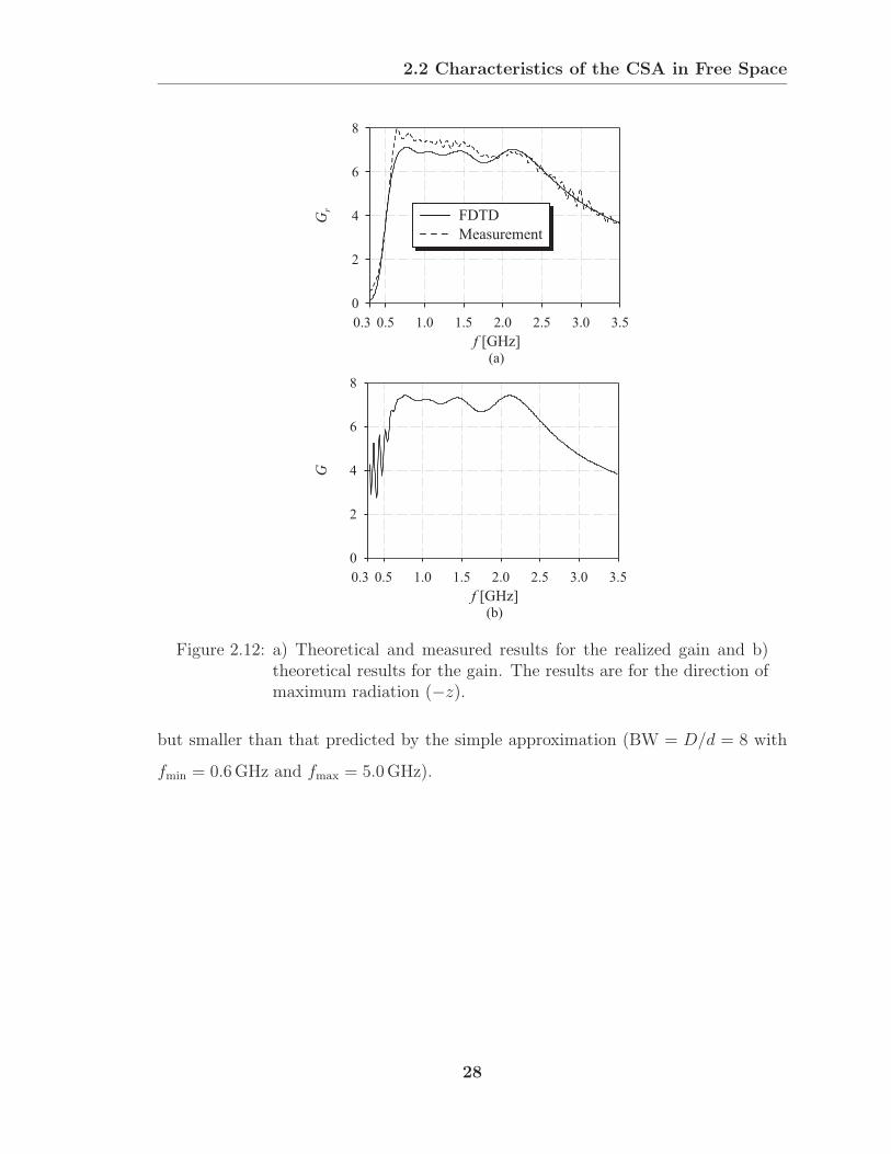
2.2 Characteristics of the CSA in Free Space
0.3 0.5 1.0 1.5 2.0 2.5 3.0 3.5
0
2
4
6
8
0.3 0.5 1.0 1.5 2.0 2.5 3.0 3.5
0
2
4
6
8
G
f [GHz](b)
f [GHz]
Gr
(a)
FDTD
Measurement
Figure 2.12: a) Theoretical and measured results for the realized gain and b)theoretical results for the gain. The results are for the direction ofmaximum radiation (−z).
but smaller than that predicted by the simple approximation (BW = D/d = 8 with
fmin = 0.6GHz and fmax = 5.0GHz).
28
CHAPTER 3
Parametric Study and Design Graphs
In this chapter, a parametric study for the unloaded CSA is performed using the
FDTD analysis. The results from this study are then used to produce design graphs,
intended to supplement and extend the graphs presented by Dyson [12]. An important
difference between the approach used here and Dyson’s is the method for determin-
ing the bandwidth of the antenna. Dyson measured the current distribution on the
antenna and determined the bandwidth from an examination of the movement of the
active region with frequency. Here, the voltage standing wave ratio (VSWR) and the
directivity are calculated, and the variation of these quantities with frequency is used
to establish the overall bandwidth.
In the parametric study, the angles that define the geometry of the antenna cover
the following ranges: 5 ≤ θ ≤ 15 and 60 ≤ α ≤ 80, with δ = 90. The remaining
parameter, the ratio of the largest diameter to the smallest diameter, D/d, is chosen
in the following manner. A simple analysis, which is presented at the end of this
chapter, shows that with the angles held fixed, the scaled bandwidth, BW/(D/d), for
a particular parameter, e.g., VSWR, is independent of the ratio D/d for sufficiently
large D/d. Thus, there is some flexibility in the choice of D/d used in the study.
Values in the range 5 ≤ D/d ≤ 7 are selected, because they make the best use of the
available computational resources.
For frequency-independent antennas, the bandwidth is often defined as the ratio
of the maximum to minimum frequencies, at which the performance of the antenna
29

Parametric Study and Design Graphs
f
Directivity
Dmax
0.0
fminDir fmax
Dir
Dmax
2
f1.0
1.5
fminVSWR fmax
VSWR
(a)
(c)
(b)
f
fminfmax
maxmin
fminfmax
maxmin
Dir Dir
Dir Dir
VSWR VSWR
VSWR VSWRRange for Hybrid Bandwidth
VSWR ( = )Z Rc
Figure 3.1: Frequencies that define various bandwidths: a) the bandwidth forVSWR, b) the bandwidth for directivity, and c) the hybrid band-width.
meets some minimum requirement: BW = fmax/fmin. Two bandwidths were exam-
ined in this study, one based on the voltage standing wave ratio, VSWR, and the
other one based on the directivity, D, in the direction for maximum radiation.1 The
bandwidth for the VSWR is obtained in the following manner. The input impedance
is determined with the antenna fed from a transmission line with Zc = R∞; here, the
overbar indicates an average over the operational bandwidth of the antenna. That is,
the characteristic impedance of the line is set equal to the average input resistance
of the infinitely-long CSA, which will discussed in more detail in Section 4.1. Briefly
stated, R∞ is the optimum resistance for the feeding transmission line to reduce the
mismatch between the line and the antenna over a wide range of frequencies. This
is also the optimum resistance to terminate the big end of the antenna in order to
1The directivity is calculated from the power density of the total field, viz, the sum of the left-
and right-handed circularly polarized components. Of course, for the left-handed CSA, the field is
predominantly left-handed circularly polarized.
30

Parametric Study and Design Graphs
reduce the end reflections. The VSWR (for Zc = R∞) is then calculated from the
input impedance,2 and, as shown in Fig. 3.1a, the bandwidth is determined from the
frequencies at which the VSWR exceeds 1.5: BWVSWR = fVSWRmax /fVSWR
min . The band-
width for the directivity is determined, as shown in Fig. 3.1b, from the frequencies
at which the directivity dropped to one half (−3 dB) of its maximum value, Dmax:
BWDir = fDirmax/fDirmin.
For the purpose of design, a single bandwidth is desirable. This was chosen
to be the region where the bandwidths for the VSWR and the directivity over-
lapped; that is, where the requirements on the VSWR and on the directivity are
met simultaneously, see Fig. 3.1c. This region is referred to as the “hybrid band-
width,” BWhybrid = fhybridmax /fhybridmin , and its limits are fhybridmin = maxfVSWRmin , fDirmin,
and fhybridmax = minfVSWRmax , fDirmax. For all cases examined in this study, it can be found
fhybridmin = fVSWRmin and fhybridmax = fDirmax. For convenience, the superscript “hybrid” will
be omitted, and the bandwidth and limiting wavelengths will be normalized in the
following manner: BW/(D/d), λmin/(πd), and λmax/(πD).
The normalized bandwidth and the limiting wavelengths are shown as functions
of the two angles θ and α based both on the VSWR, Fig. 3.2, and on the directivity,
Fig. 3.3. Figure 3.4 is for the combination of the two, i.e., for the hybrid results. In
these design graphs, the light gray areas bounded by solid lines are the results from
this study, and the dark gray areas bounded by dashed lines are Dyson’s results. For
clarity, only the curves for α = 60 and 80 are shown; linear interpolation can be used
between these two values. When the shortest and largest limiting wavelengths for the
results based on the VSWR and the directivity are compared, Figs. 3.2 and 3.3, they
2It is not necessary to perform a separate FDTD calculation just to determine the VSWR for a
particular characteristic impedance when the VSWR for the same antenna is already known for a
different characteristic impedance. In both cases, the input impedance must be the same since it is
independent of the characteristic impedance of the feeding line when the simple FDTD feed model
is used. Simple transmission-line equations can then be used to renormalize the existing VSWR to
any characteristic impedance.
31
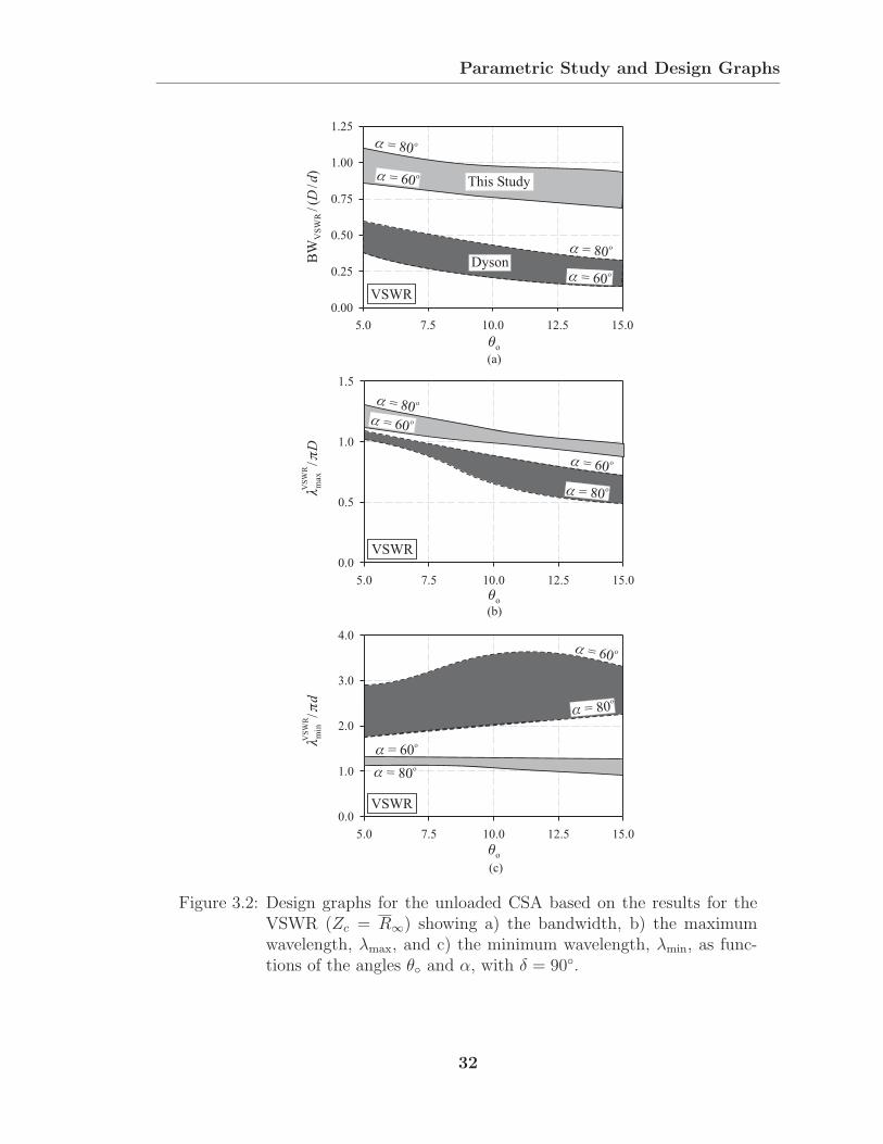
Parametric Study and Design Graphs
5.0 7.5 10.0 12.5 15.0
0.00
0.25
0.50
0.75
1.00
1.25
= 80o
= 60oThis Study
Dyson = 60
o
= 80o
5.0 7.5 10.0 12.5 15.0
0.0
1.0
2.0
3.0
4.0
o
o
BW
/(/
)V
SW
RD
d
m
in/
d
= 80o
= 80o
= 60o
= 60 o
5.0 7.5 10.0 12.5 15.0
0.0
0.5
1.0
1.5
o
max
/D
= 60o
= 80 o
= 80o
(a)
(b)
(c)
= 60o
VS
WR
VS
WR
VSWR
VSWR
VSWR
Figure 3.2: Design graphs for the unloaded CSA based on the results for theVSWR (Zc = R∞) showing a) the bandwidth, b) the maximumwavelength, λmax, and c) the minimum wavelength, λmin, as func-tions of the angles θ and α, with δ = 90.
32
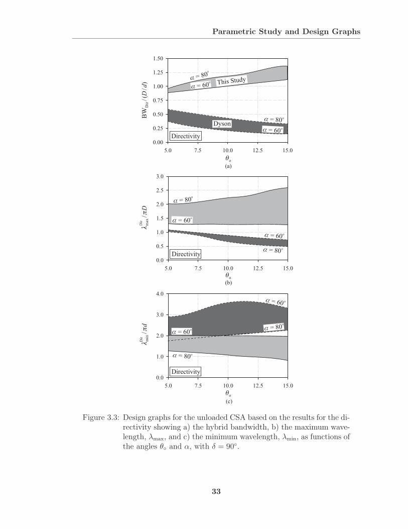
Parametric Study and Design Graphs
5.0 7.5 10.0 12.5 15.0
0.0
0.5
1.0
1.5
2.0
2.5
3.0
= 80o
= 60o
= 60o
= 80o
5.0 7.5 10.0 12.5 15.0
0.00
0.25
0.50
0.75
1.00
1.25
1.50
Dyson = 80
o
= 60o
= 80o
= 60o This Study
o
o
BW
/(/
)D
irD
d
m
in/
d
o
max/
D
(a)
(b)
(c)
5.0 7.5 10.0 12.5 15.0
0.0
1.0
2.0
3.0
4.0
= 80o
= 80o
= 60 o
= 60o
Dir
Dir
Directivity
Directivity
Directivity
Figure 3.3: Design graphs for the unloaded CSA based on the results for the di-rectivity showing a) the hybrid bandwidth, b) the maximum wave-length, λmax, and c) the minimum wavelength, λmin, as functions ofthe angles θ and α, with δ = 90.
33

Parametric Study and Design Graphs
5.0 7.5 10.0 12.5 15.0
0.0
1.0
2.0
3.0
4.0
5.0 7.5 10.0 12.5 15.0
0.00
0.25
0.50
0.75
1.00
o
o
BW
/(/
)D
d
m
in/
d
= 80o
= 80o
= 80o
= 80o
= 60o
= 60o
= 60o
= 60 o
5.0 7.5 10.0 12.5 15.0
0.0
0.5
1.0
1.5
o
max/
D
= 60o
= 80 o
= 80o
= 60o
This Study
Dyson
(a)
(b)
(c)
Hybrid
Hybrid
Hybrid
Figure 3.4: Design graphs for the unloaded CSA showing a) the hybrid band-width, b) the maximum wavelength, λmax, and c) the minimumwavelength, λmin, as functions of the angles θ and α, with δ = 90.
34

Parametric Study and Design Graphs
o
5.0 7.5 10.0 12.5 15.0
0
25
50
75
100
125
150
175
= 80o
Dyson
= 80o
= 60o
This Study
|X |
= 60o
R|X
|,
[]
R R
Figure 3.5: Design graph for the unloaded CSA showing the average inputimpedance of the infinitely-long CSA as a function of the anglesθ and α, with δ = 90.
are seen to extend over different ranges. As illustrated qualitatively in Fig. 3.1, the
operational range of the antenna based on the directivity is shifted towards larger
wavelengths/lower frequencies relative to the range based on the VSWR. In both
these cases, the simplest approximation for the bandwidth, discussed in Section 2.1,
describes the performance of the CSA pretty well, i.e., BWVSWR ≈ BWDir ≈ D/d.
Also notice, that the range of acceptable performance is significantly wider than that
suggested by Dyson. The hybrid results from this study, Fig. 3.4, indicate a useful
bandwidth that is at least 50% greater than that proposed by Dyson. In this case,
the simple approximation, BW = D/d, clearly overestimates the bandwidth.
In Figs. 3.5-3.7, each of the parameters displayed was obtained by averaging
over the hybrid bandwidth. Figure 3.5 shows the average input impedance, R∞ and
|X∞|, of the infinitely long CSA as a function of the angle θ with the angle α as a
parameter. For the ranges displayed, both of these angles are seen to have very little
effect on the input impedance. The input resistance is R∞ ≈ 150Ω, and the reactance
is small, |X∞| < 25Ω. It is important to mention that the input resistance of the CSA
of finite length, averaged over the hybrid bandwidth, that is R, is essentially the same
as the average resistance for the infinitely long CSA, R∞. Hence, for the purposes of
35

Parametric Study and Design Graphs
design, Fig. 3.5 can be used as a graph for the input impedance of the CSA of finite
length: Z = R + jX ≈ R∞, since |X| R. The three values of measured input
resistance from Dyson’s work (solid dots) are seen to agree with the values from this
study.
Figure 3.6 shows three characteristics of the pattern of the CSA: the average
directivity in the direction for maximum radiation (−z), D, the average half-power
beamwidth, HPBW, averaged over two orthogonal planes (φ = 0 and φ = 90), and
the front-to-back ratio, FTBR.3 These quantities are plotted as functions of the angle
θ with the angle α as parameter. Note that the directivity is plotted on a linear scale,
and the front-to-back ratio is plotted on a logarithmic scale. Again, the solid lines
are the results from this study, and the dashed lines are Dyson’s results. The average
directivity for this study exceeds that from Dyson’s study; the same is true for the
half-power beamwidth, which agree better with Dyson’s results if the results for this
study are averaged over Dyson’s bandwidth.
The state of polarization is given by the axial ratio, AR. The average axial ratio
for the electric field in the direction of maximum radiation (−z) is shown in Fig. 3.7.
For circular polarization AR = 1.0. Clearly, as the sketches for the polarization ellipse
at the two extremes show, the radiation is very nearly circularly polarized over the
whole range of angles displayed.
All of the design graphs, Figs. 3.2-3.7, show that the best performance is ob-
tained from the CSA when the angle of the cone, θ, is small, and the arms are tightly
wrapped, viz, the angle α is close to 90.
The following analysis shows that the results for the normalized bandwidth,
BW/(D/d), and limiting wavelengths, λmax/(πD) and λmin/(πd), are independent of
the ratio of biggest to smallest cone diameter, D/d. To show that these results hold
for any D/d, if chosen sufficiently large, the performance characteristics VSWR and
directivity are examined for three different CSA geometries and for three different
3All of these quantities are calculated from the power density of the total field, viz, the sum of
the left-handed and right-handed circularly polarized components.
36

Parametric Study and Design Graphs
5.0 7.5 10.0 12.5 15.0
0
2
4
6
8
10
= 60o
= 80 o
= 60 o
= 80 o
5.0 7.5 10.0 12.5 15.0
1
1
0
20
30
40
o
FT
BR
[dB
]
= 80 o
D
o
This Study
Dyson
5.0 7.5 10.0 12.5 15
=
60 o
.0
0
45
90
135
180
o
= 60o = 60
o
= 80o = 80
o
HP
BW
[Deg
.]
(a)
(b)
(c)
Figure 3.6: Design graphs for the unloaded CSA showing a) the average di-rectivity, b) the average half-power beamwidth, and c) the averagefront-to-back ratio as functions of angles θ and α, with δ = 90.
37
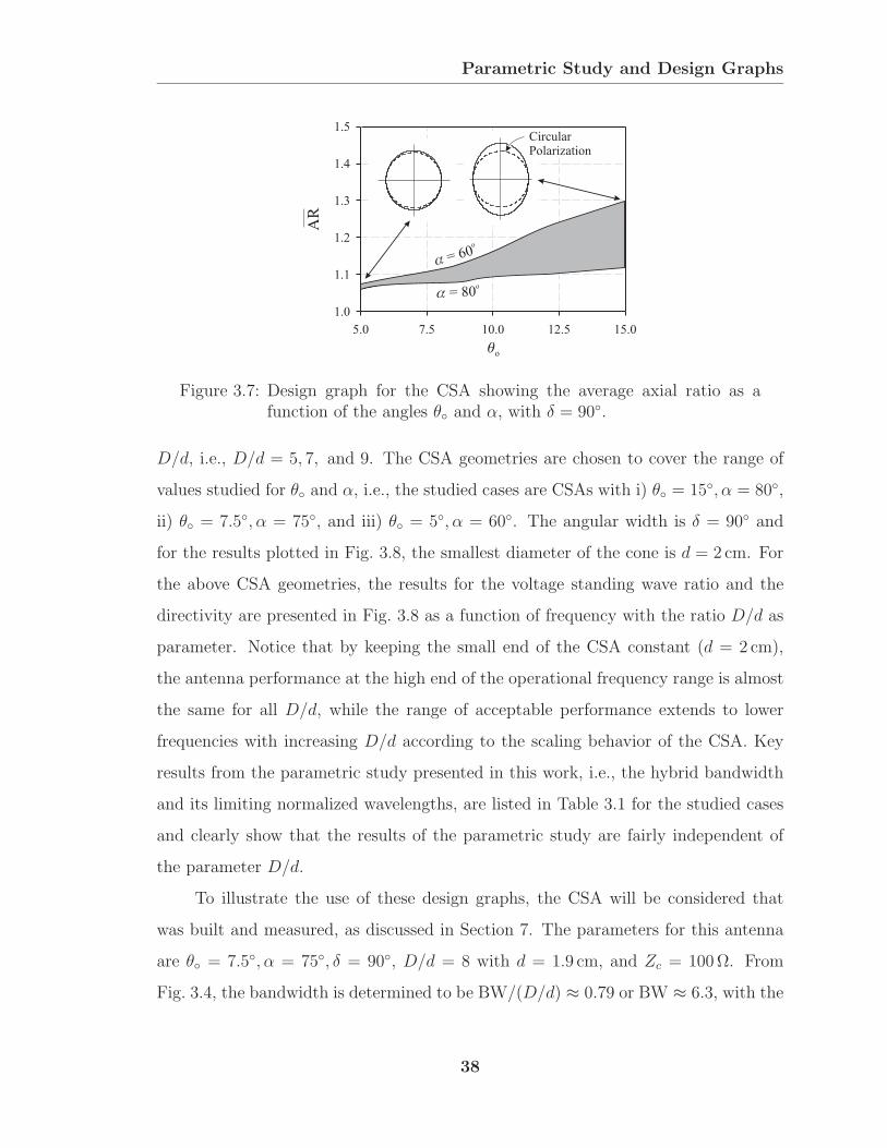
Parametric Study and Design Graphs
o
AR
5.0 7.5 10.0 12.5 15.0
1.0
1.1
1.2
1.3
1.4
1.5
= 80o
= 60o
CircularPolarization
Figure 3.7: Design graph for the CSA showing the average axial ratio as afunction of the angles θ and α, with δ = 90.
D/d, i.e., D/d = 5, 7, and 9. The CSA geometries are chosen to cover the range of
values studied for θ and α, i.e., the studied cases are CSAs with i) θ = 15, α = 80,
ii) θ = 7.5, α = 75, and iii) θ = 5, α = 60. The angular width is δ = 90 and
for the results plotted in Fig. 3.8, the smallest diameter of the cone is d = 2 cm. For
the above CSA geometries, the results for the voltage standing wave ratio and the
directivity are presented in Fig. 3.8 as a function of frequency with the ratio D/d as
parameter. Notice that by keeping the small end of the CSA constant (d = 2 cm),
the antenna performance at the high end of the operational frequency range is almost
the same for all D/d, while the range of acceptable performance extends to lower
frequencies with increasing D/d according to the scaling behavior of the CSA. Key
results from the parametric study presented in this work, i.e., the hybrid bandwidth
and its limiting normalized wavelengths, are listed in Table 3.1 for the studied cases
and clearly show that the results of the parametric study are fairly independent of
the parameter D/d.
To illustrate the use of these design graphs, the CSA will be considered that
was built and measured, as discussed in Section 7. The parameters for this antenna
are θ = 7.5, α = 75, δ = 90, D/d = 8 with d = 1.9 cm, and Zc = 100Ω. From
Fig. 3.4, the bandwidth is determined to be BW/(D/d) ≈ 0.79 or BW ≈ 6.3, with the
38

Parametric Study and Design Graphs
f [GHz]
f [GHz]
f [GHz]
f [GHz]
f [GHz]
f [GHz]
0.4 1.0 2.0 3.0 4.0
0
1
2
3
4
5
0.4 1.0 2.0 3.0 4.0
0
2
4
6
8
0.3 1.0 2.0 3.0 4.0
0
1
2
3
4
5
0.3 1.0 2.0 3.0 4.0
0
2
4
6
8
0.2 1.0 2.0 3.0 4.0
0
1
2
3
4
5
0.2 1.0 2.0 3.0 4.0
0
2
4
6
D dD dD d
/ = 5/ = 7/ = 9
D dD dD d
/ = 5/ = 7/ = 9
VS
WR
VS
WR
VS
WR
DD
D
(a) (b)
(c) (d)
(e) (f)
Figure 3.8: Theoretical results for the VSWR (a,c,e) and the directivity (b,d,f)as a function of frequency with D/d as parameter. The results arefor a CSA with a) and b) θ = 15, α = 80, δ = 90, c) and d)θ = 7.5, α = 75, δ = 90, and e) and f) θ = 5, α = 60, δ = 90.
39
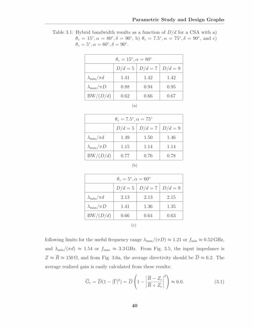
Parametric Study and Design Graphs
Table 3.1: Hybrid bandwidth results as a function of D/d for a CSA with a)θ = 15, α = 80, δ = 90, b) θ = 7.5, α = 75, δ = 90, and c)θ = 5, α = 60, δ = 90.
θ = 15, α = 80
D/d = 5 D/d = 7 D/d = 9
λmin/πd 1.41 1.42 1.42
λmax/πD 0.88 0.94 0.95
BW/(D/d) 0.62 0.66 0.67
(a)
θ = 7.5, α = 75
D/d = 5 D/d = 7 D/d = 9
λmin/πd 1.49 1.50 1.46
λmax/πD 1.15 1.14 1.14
BW/(D/d) 0.77 0.76 0.78
(b)
θ = 5, α = 60
D/d = 5 D/d = 7 D/d = 9
λmin/πd 2.13 2.13 2.15
λmax/πD 1.41 1.36 1.35
BW/(D/d) 0.66 0.64 0.63
(c)
following limits for the useful frequency range λmax/(πD) ≈ 1.21 or fmin ≈ 0.52GHz,
and λmin/(πd) ≈ 1.54 or fmax ≈ 3.3GHz. From Fig. 3.5, the input impedance is
Z ≈ R ≈ 150Ω, and from Fig. 3.6a, the average directivity should be D ≈ 6.2. The
average realized gain is easily calculated from these results:
Gr = D(1− |Γ|2) = D
1−
∣∣∣∣∣R− Zc
R + Zc
∣∣∣∣∣2 ≈ 6.0. (3.1)
40

Parametric Study and Design Graphs
Now these predictions can be compared with the measured results in Figs. 7.21 and
2.12a. Both the prediction for the resistance and the prediction for the realized gain
are seen to be close to the measured values when the latter are averaged over the
specified frequency range: 0.52GHz ≤ f ≤ 3.3GHz.
41
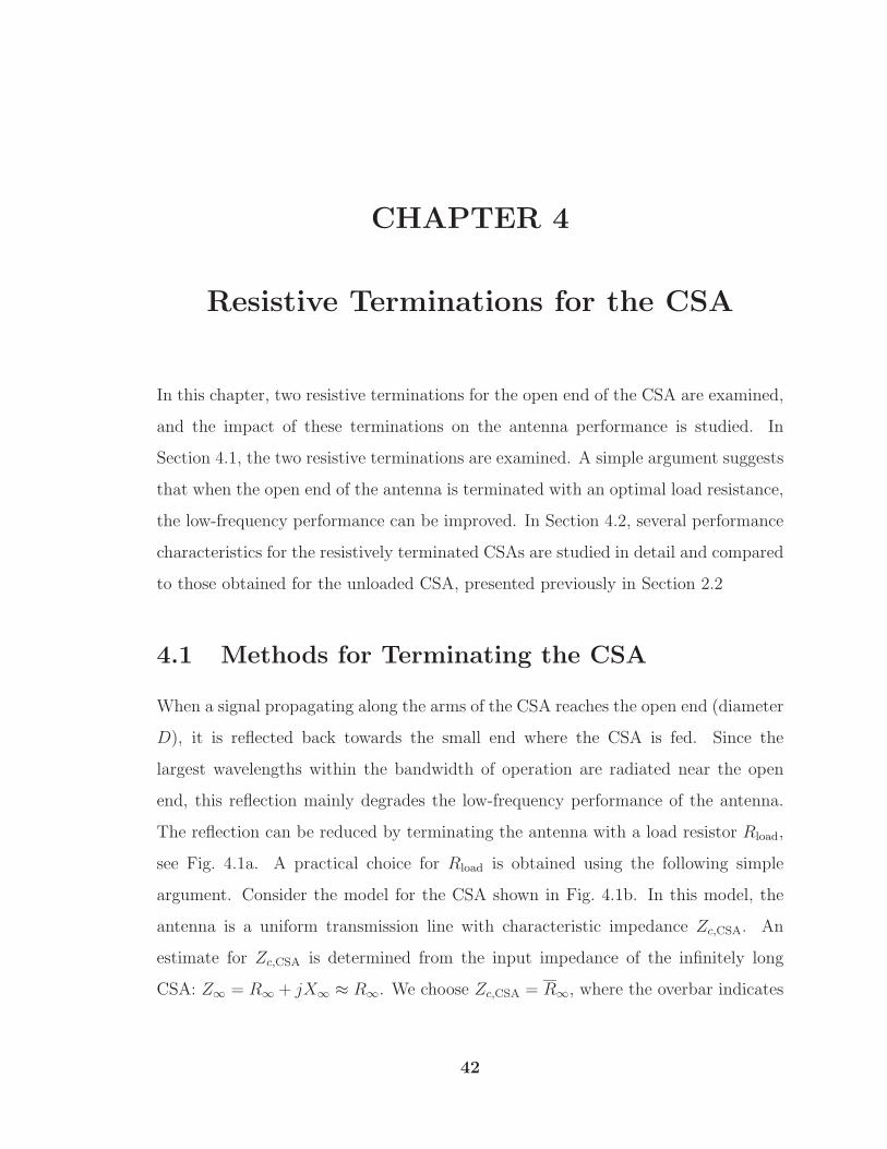
CHAPTER 4
Resistive Terminations for the CSA
In this chapter, two resistive terminations for the open end of the CSA are examined,
and the impact of these terminations on the antenna performance is studied. In
Section 4.1, the two resistive terminations are examined. A simple argument suggests
that when the open end of the antenna is terminated with an optimal load resistance,
the low-frequency performance can be improved. In Section 4.2, several performance
characteristics for the resistively terminated CSAs are studied in detail and compared
to those obtained for the unloaded CSA, presented previously in Section 2.2
4.1 Methods for Terminating the CSA
When a signal propagating along the arms of the CSA reaches the open end (diameter
D), it is reflected back towards the small end where the CSA is fed. Since the
largest wavelengths within the bandwidth of operation are radiated near the open
end, this reflection mainly degrades the low-frequency performance of the antenna.
The reflection can be reduced by terminating the antenna with a load resistor Rload,
see Fig. 4.1a. A practical choice for Rload is obtained using the following simple
argument. Consider the model for the CSA shown in Fig. 4.1b. In this model, the
antenna is a uniform transmission line with characteristic impedance Zc,CSA. An
estimate for Zc,CSA is determined from the input impedance of the infinitely long
CSA: Z∞ = R∞ + jX∞ ≈ R∞. We choose Zc,CSA = R∞, where the overbar indicates
42
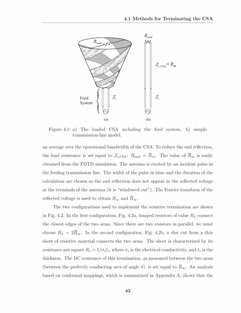
4.1 Methods for Terminating the CSA
Zc
Rload
Zc
Rload
(a) (b)
FeedSystem
RZc,CSA
Figure 4.1: a) The loaded CSA including the feed system, b) simpletransmission-line model.
an average over the operational bandwidth of the CSA. To reduce the end reflection,
the load resistance is set equal to Zc,CSA: Rload = R∞. The value of R∞ is easily
obtained from the FDTD simulation. The antenna is excited by an incident pulse in
the feeding transmission line. The width of the pulse in time and the duration of the
calculation are chosen so the end reflection does not appear in the reflected voltage
at the terminals of the antenna (it is “windowed out”). The Fourier transform of the
reflected voltage is used to obtain R∞ and R∞.
The two configurations used to implement the resistive termination are shown
in Fig. 4.2. In the first configuration, Fig. 4.2a, lumped resistors of value RL connect
the closest edges of the two arms. Since there are two resistors in parallel, we must
choose RL = 2R∞. In the second configuration, Fig. 4.2b, a disc cut from a thin
sheet of resistive material connects the two arms. The sheet is characterized by its
resistance per square Rs = 1/σsts, where σs is the electrical conductivity, and ts is the
thickness. The DC resistance of this termination, as measured between the two arms
(between the perfectly conducting arcs of angle δ), is set equal to R∞. An analysis
based on conformal mappings, which is summarized in Appendix A, shows that the
43

4.2 Characteristics of the Loaded CSAs
Resistive Sheet
D
Rs sts
1=
(b)
LumpedResistor
y
x
z
Spiral Arms
RL
RL
(a)
Figure 4.2: Schematic drawings for the two resistive terminations: a) twolumped resistors connecting the ends of the spiral arms, b) a re-sistive sheet covering the entire end of the cone.
resistance per square should be
Rs = R∞K
(k =
√1− u42
)2K(k = u22)
, (4.1)
where K(k) is the complete elliptic integral of first kind with the modulus k, and
u2 =cos(δ/2)
1 + sin(δ/2). (4.2)
For the case of interest in this work, δ = 90, (4.1) simplifies to become Rs = R∞.
4.2 Characteristics of the Loaded CSAs
In this section, several performance characteristics are presented for the CSA ter-
minated resistively using lumped resistors and a resistive sheet. The objective is
to study the effect of these terminations on the performance of the loaded CSAs
and to compare the performance to that of the unloaded CSA. As in Section 2.2,
the results presented are for the left-handed CSA with the following parameters:
θ = 7.5, α = 75, δ = 90, D/d = 8 with d = 1.9 cm, and Zc = 100Ω.
In order to properly study the performance characteristics of the CSA with
resistive terminations, it is necessary to determine the most practical load resistance,
Rload = R∞, first. The following analysis outlines the technique introduced in Section
44

4.2 Characteristics of the Loaded CSAs
4.1, i.e., to obtain R∞ with a FDTD simulation. For the drive-point response of
the practical CSA to resemble that of the infinite CSA, the voltage measured at the
drive-point terminals must only contain the drive-point reflection. It is therefore
necessary to choose an incident signal with finite and sufficiently narrow temporal
extent to guarantee that drive-point reflection for the unloaded CSA vanishes well
before the first end reflection arrives at t/τL = 2. The differentiated Gaussian voltage
pulse, introduced in Section 2.2, with τp/τL = 1.6 · 10−2 is a good choice, because itsufficiently satisfies above criterion, see Fig. 2.5. The result for the reflected voltage
of such a FDTD simulation is shown in Fig. 4.3a as a function of normalized time,
t/τL, which is almost identical to the reflected voltage in Fig. 2.5 but with all signals
arriving later than the drive-point reflection windowed out, i.e., setting the voltage
to zero for t/τL ≥ 1. Ideally, this signal is the voltage response of the infinitely
long CSA and thus sufficient to determine the input impedance of the infinite CSA,
Z∞ = R∞ + jX∞, which is shown as a function of frequency in Fig. 4.3b. Evidently,
the resistance is almost constant and the reactance is small over the frequency range
displayed, i.e., |X∞| R∞. The load resistance minimizing the reflection from the
big end of the antenna is now approximated by the average resistance over the hybrid
frequency range, i.e., Rload = R∞ ≈ 150Ω.1 Thus, the CSA terminated with lumped
resistors, see Fig. 4.2a, should have RL ≈ 300Ω, while the CSA terminated with a
resistive sheet, see Fig. 4.2b, should have Rs ≈ 150Ω.
The first result for the CSA with and without resistive terminations is for the
reflected voltage as a function of normalized time, t/τL, with τp/τL = 1.6 · 10−2.The solid line in Fig. 4.4 is for the unloaded antenna, the dashed line is for the
CSA terminated with two lumped resistors, and the dash-dotted line is for the CSA
terminated with a resistive sheet. As expected, the drive-point reflection at t/τL ≈ 0
is the same for all cases. It can be seen that the terminations significantly reduce the
reflections from the antenna end. The amplitude of the reflected pulse at t = 2τL for
1Recall that the results for this resistance, R∞, are presented for CSAs with 5 ≤ θ ≤ 15, 60 ≤α ≤ 80 and δ = 90 in Fig. 3.5.
45
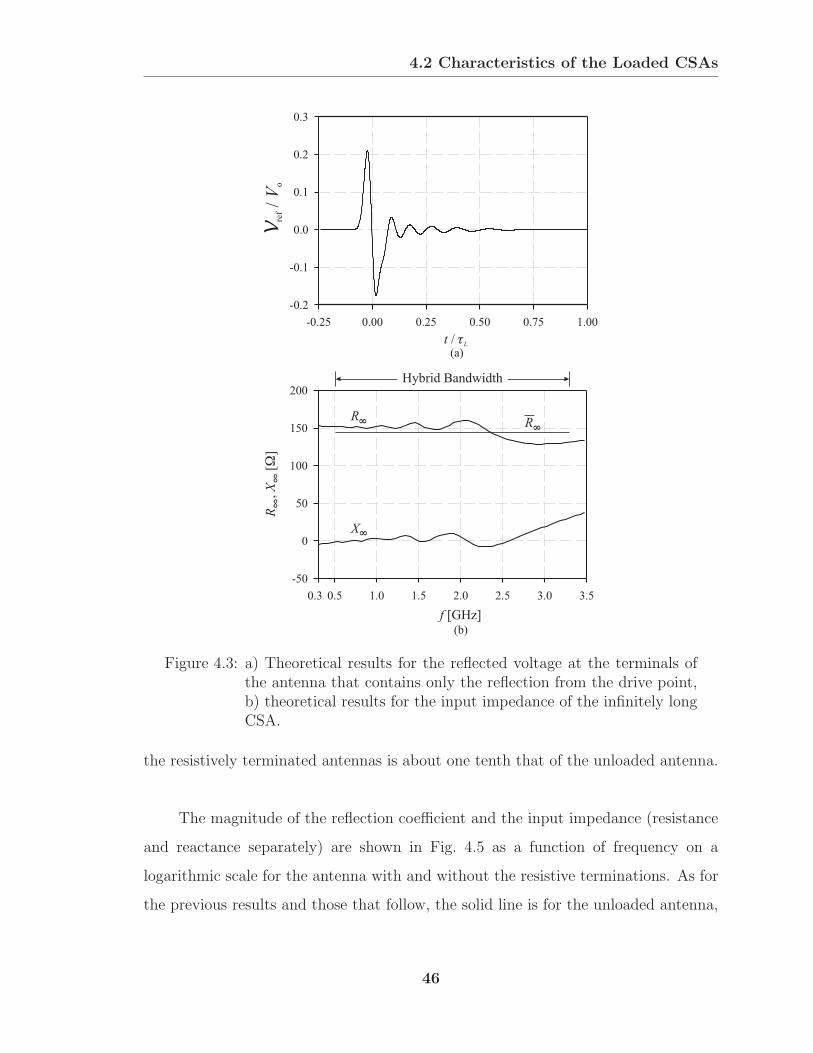
4.2 Characteristics of the Loaded CSAs
-0.25 0.00 0.25 0.50 0.75 1.00
-0.2
-0.1
0.0
0.1
0.2
0.3
0.3 0.5 1.0 1.5 2.0 2.5 3.0 3.5
-50
0
50
100
150
200
t / L
Vre
fo
/V
f [GHz]
X
RR
(a)
(b)
Hybrid Bandwidth
RX
,[
]
Figure 4.3: a) Theoretical results for the reflected voltage at the terminals ofthe antenna that contains only the reflection from the drive point,b) theoretical results for the input impedance of the infinitely longCSA.
the resistively terminated antennas is about one tenth that of the unloaded antenna.
The magnitude of the reflection coefficient and the input impedance (resistance
and reactance separately) are shown in Fig. 4.5 as a function of frequency on a
logarithmic scale for the antenna with and without the resistive terminations. As for
the previous results and those that follow, the solid line is for the unloaded antenna,
46
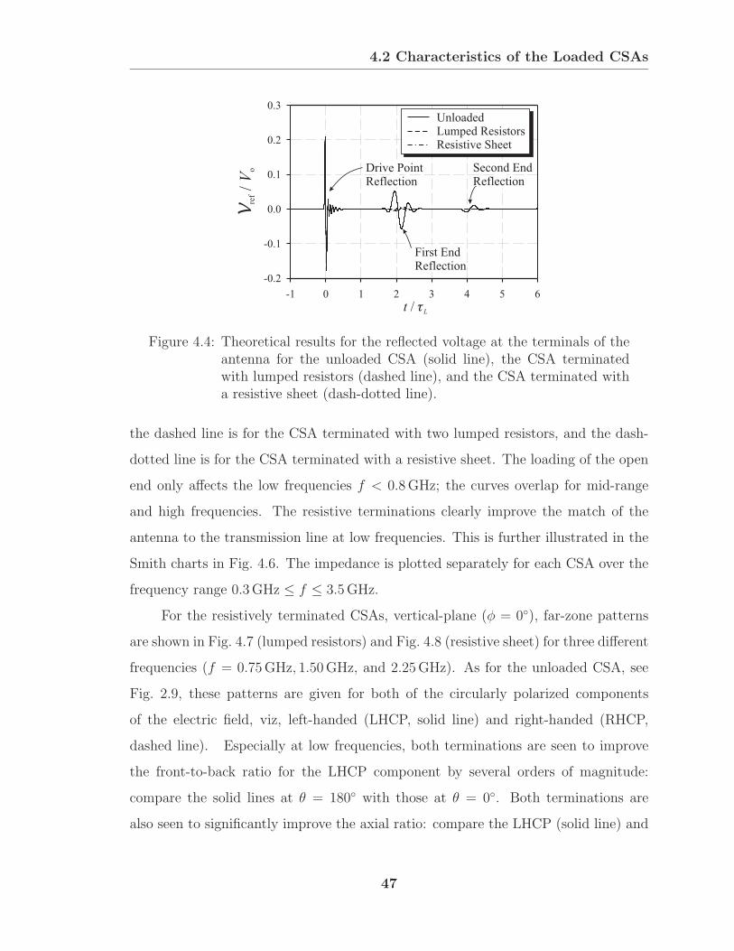
4.2 Characteristics of the Loaded CSAs
-1 0 1 2 3 4 5 6
-0.2
-0.1
0.0
0.1
0.2
0.3
t / L
Vre
fo
/V
Drive PointReflection
Second EndReflection
First EndReflection
UnloadedLumped ResistorsResistive Sheet
Figure 4.4: Theoretical results for the reflected voltage at the terminals of theantenna for the unloaded CSA (solid line), the CSA terminatedwith lumped resistors (dashed line), and the CSA terminated witha resistive sheet (dash-dotted line).
the dashed line is for the CSA terminated with two lumped resistors, and the dash-
dotted line is for the CSA terminated with a resistive sheet. The loading of the open
end only affects the low frequencies f < 0.8GHz; the curves overlap for mid-range
and high frequencies. The resistive terminations clearly improve the match of the
antenna to the transmission line at low frequencies. This is further illustrated in the
Smith charts in Fig. 4.6. The impedance is plotted separately for each CSA over the
frequency range 0.3GHz ≤ f ≤ 3.5GHz.
For the resistively terminated CSAs, vertical-plane (φ = 0), far-zone patterns
are shown in Fig. 4.7 (lumped resistors) and Fig. 4.8 (resistive sheet) for three different
frequencies (f = 0.75GHz, 1.50GHz, and 2.25GHz). As for the unloaded CSA, see
Fig. 2.9, these patterns are given for both of the circularly polarized components
of the electric field, viz, left-handed (LHCP, solid line) and right-handed (RHCP,
dashed line). Especially at low frequencies, both terminations are seen to improve
the front-to-back ratio for the LHCP component by several orders of magnitude:
compare the solid lines at θ = 180 with those at θ = 0. Both terminations are
also seen to significantly improve the axial ratio: compare the LHCP (solid line) and
47
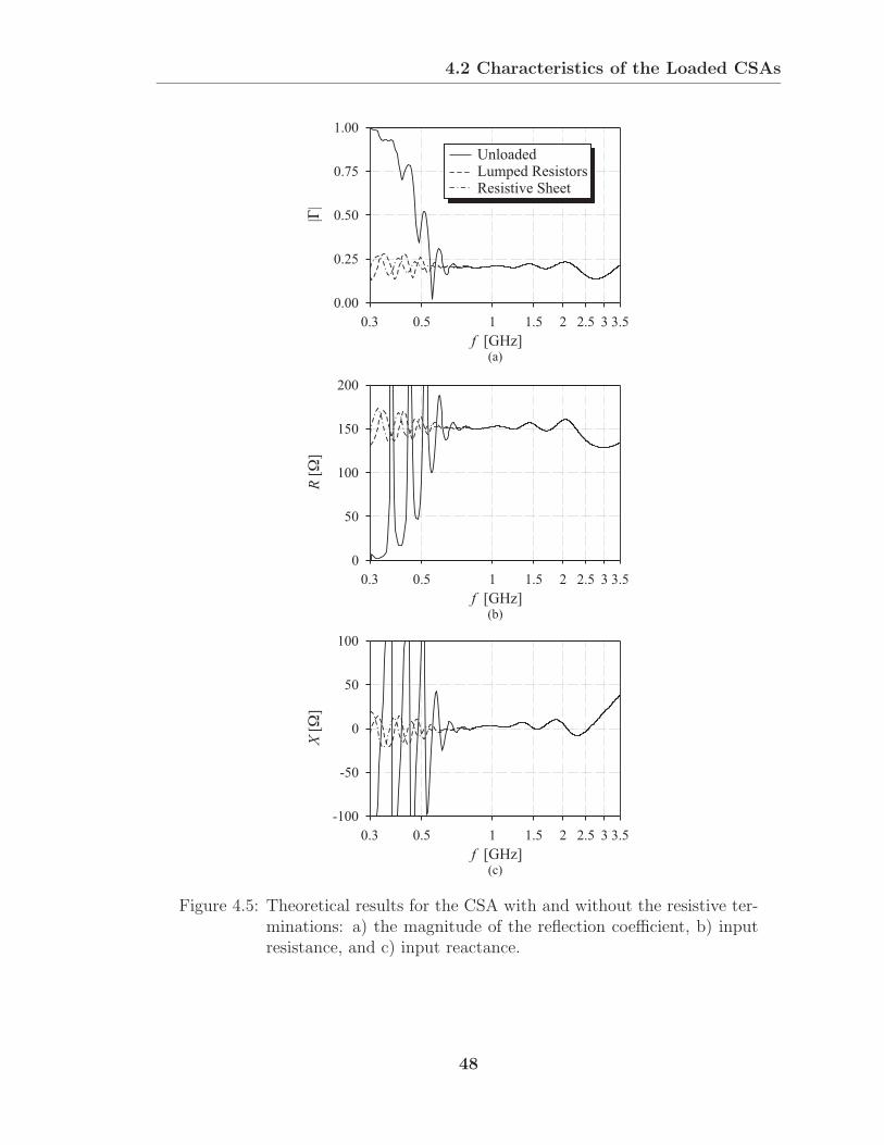
4.2 Characteristics of the Loaded CSAs
f [GHz]
||
(a)
0.3 0.5 1 1.5 2 2.5 3 3.5
0.00
0.25
0.50
0.75
1.00
f [GHz]
R[
]
(b)
0.3 0.5 1 1.5 2 2.5 3 3.5
0
50
100
150
200
f [GHz]
X[
]
(c)
0.3 0.5 1 1.5 2 2.5 3 3.5
-100
-50
0
50
100
UnloadedLumped ResistorsResistive Sheet
Figure 4.5: Theoretical results for the CSA with and without the resistive ter-minations: a) the magnitude of the reflection coefficient, b) inputresistance, and c) input reactance.
48

4.2 Characteristics of the Loaded CSAs
j 2
-j 2
j 1
-j 1
j 0.2
-j 0.2
j 0.5
-j 0.5
j 2
-j 2
j 1
-j 1
j 0.2
-j 0.2
j 0.5
-j 0.5
j 2
-j 2
j 1
-j 1
j 0.2
-j 0.2
j 0.5
-j 0.5
(a)
(b)
(c)
0 1 2 50.50.2
0 1 2 50.50.2
0 1 2 50.50.2
Figure 4.6: Smith charts for a) the unloaded CSA, b) the CSA terminated withlumped resistors, and c) the CSA terminated with a resistive sheet.
49
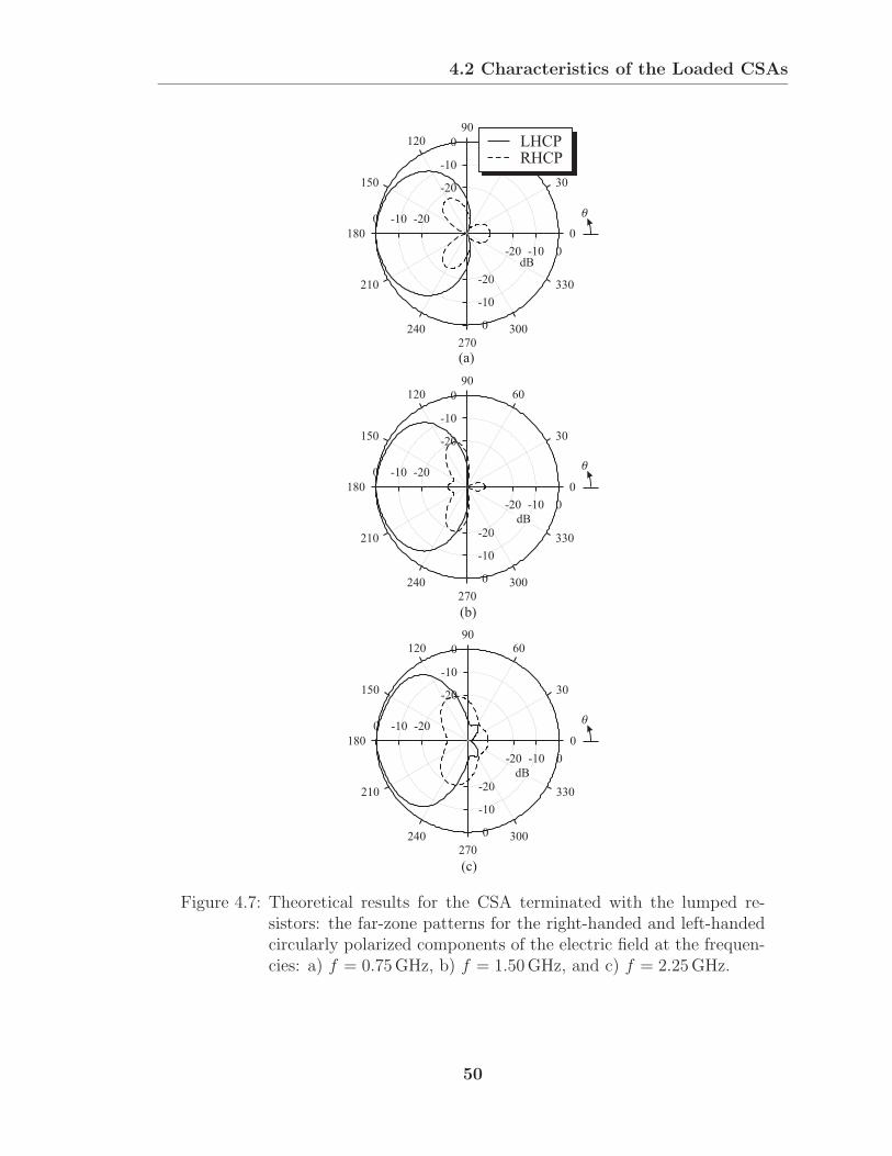
4.2 Characteristics of the Loaded CSAs
0-10-20
0
-10
-20
0 -10 -20
0
-10
-20
0
30
6090
120
150
180
210
240270
300
330
0-10-20
0
-10
-20
0 -10 -20
0
-10
-20
0
30
6090
120
150
180
210
240270
300
330
LHCPRHCP
dB
(a)
0-10-20
0
-10
-20
0 -10 -20
0
-10
-20
0
30
6090
120
150
180
210
240270
300
330
dB
(b)
(c)
dB
Figure 4.7: Theoretical results for the CSA terminated with the lumped re-sistors: the far-zone patterns for the right-handed and left-handedcircularly polarized components of the electric field at the frequen-cies: a) f = 0.75GHz, b) f = 1.50GHz, and c) f = 2.25GHz.
50

4.2 Characteristics of the Loaded CSAs
0-10-20
0
-10
-20
0 -10 -20
0
-10
-20
0
30
6090
120
150
180
210
240270
300
330
0-10-20
0
-10
-20
0 -10 -20
0
-10
-20
0
30
6090
120
150
180
210
240270
300
330
LHCPRHCP
dB
dB
(a)
(b)
0-10-20
0
-10
-20
0 -10 -20
0
-10
-20
0
30
6090
120
150
180
210
240270
300
330
(c)
dB
Figure 4.8: Theoretical results for the CSA terminated with a resistive sheet:the far-zone patterns for the right-handed and left-handed circularlypolarized components of the electric field at the frequencies: a)f = 0.75GHz, b) f = 1.50GHz, and c) f = 2.25GHz.
51
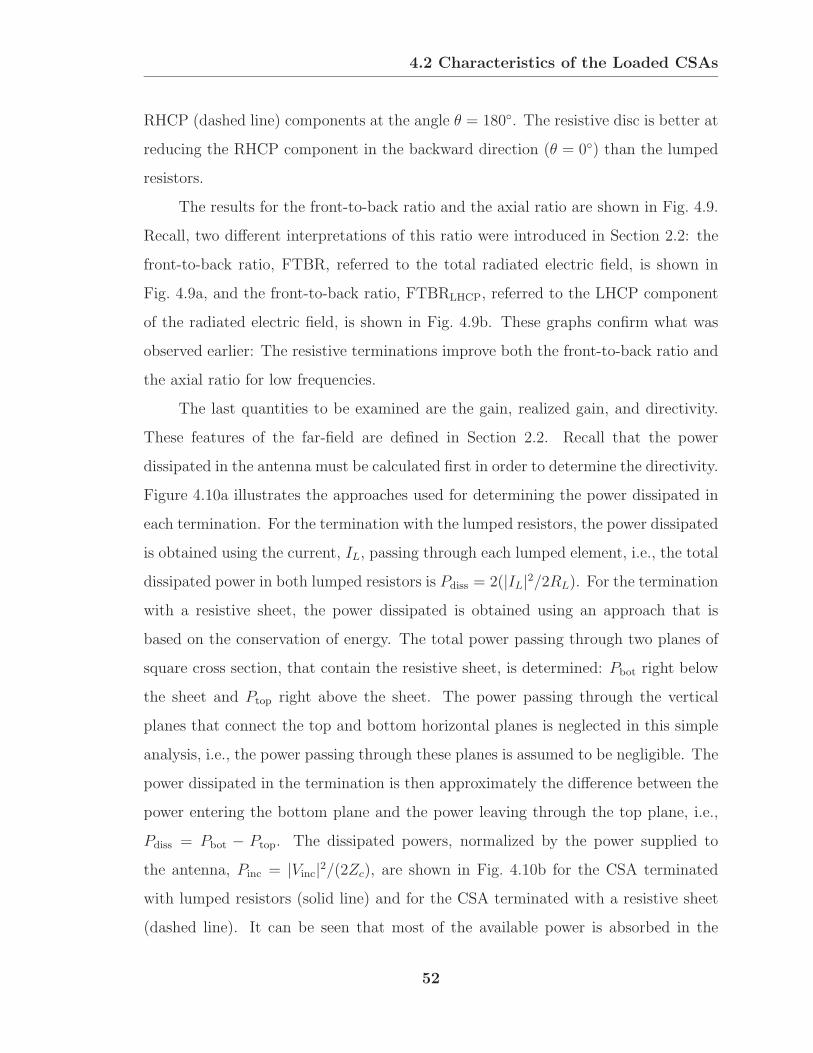
4.2 Characteristics of the Loaded CSAs
RHCP (dashed line) components at the angle θ = 180. The resistive disc is better at
reducing the RHCP component in the backward direction (θ = 0) than the lumped
resistors.
The results for the front-to-back ratio and the axial ratio are shown in Fig. 4.9.
Recall, two different interpretations of this ratio were introduced in Section 2.2: the
front-to-back ratio, FTBR, referred to the total radiated electric field, is shown in
Fig. 4.9a, and the front-to-back ratio, FTBRLHCP, referred to the LHCP component
of the radiated electric field, is shown in Fig. 4.9b. These graphs confirm what was
observed earlier: The resistive terminations improve both the front-to-back ratio and
the axial ratio for low frequencies.
The last quantities to be examined are the gain, realized gain, and directivity.
These features of the far-field are defined in Section 2.2. Recall that the power
dissipated in the antenna must be calculated first in order to determine the directivity.
Figure 4.10a illustrates the approaches used for determining the power dissipated in
each termination. For the termination with the lumped resistors, the power dissipated
is obtained using the current, IL, passing through each lumped element, i.e., the total
dissipated power in both lumped resistors is Pdiss = 2(|IL|2/2RL). For the termination
with a resistive sheet, the power dissipated is obtained using an approach that is
based on the conservation of energy. The total power passing through two planes of
square cross section, that contain the resistive sheet, is determined: Pbot right below
the sheet and Ptop right above the sheet. The power passing through the vertical
planes that connect the top and bottom horizontal planes is neglected in this simple
analysis, i.e., the power passing through these planes is assumed to be negligible. The
power dissipated in the termination is then approximately the difference between the
power entering the bottom plane and the power leaving through the top plane, i.e.,
Pdiss = Pbot − Ptop. The dissipated powers, normalized by the power supplied to
the antenna, Pinc = |Vinc|2/(2Zc), are shown in Fig. 4.10b for the CSA terminated
with lumped resistors (solid line) and for the CSA terminated with a resistive sheet
(dashed line). It can be seen that most of the available power is absorbed in the
52
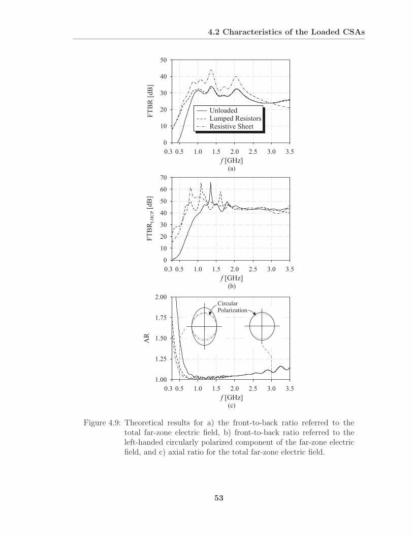
4.2 Characteristics of the Loaded CSAs
(a)
FT
BR
[dB
]
f [GHz]
0.3 0.5 1.0 1.5 2.0 2.5 3.0 3.5
0
10
20
30
40
50
FT
BR
LH
CP
[dB
]
f [GHz](b)
0.3 0.5 1.0 1.5 2.0 2.5 3.0 3.5
0
10
20
30
40
50
60
70
UnloadedLumped ResistorsResistive Sheet
AR
f [GHz](c)
0.3 0.5 1.0 1.5 2.0 2.5 3.0 3.5
1.00
1.25
1.50
1.75
2.00CircularPolarization
Figure 4.9: Theoretical results for a) the front-to-back ratio referred to thetotal far-zone electric field, b) front-to-back ratio referred to theleft-handed circularly polarized component of the far-zone electricfield, and c) axial ratio for the total far-zone electric field.
53
4.2 Characteristics of the Loaded CSAs
IL
ILPbot
PtopSide View:
Top View:
RL
RLCircular ResistiveSheet
(a)
(c)
f [GHz]
0.3 0.5 1.0 1.5 2.0 2.5 3.0 3.5
0.00
0.25
0.50
0.75
1.00
1.25
(b)
f [GHz]
PP
dis
sin
c/
0.3 0.5 1.0 1.5 2.0 2.5 3.0 3.5
0.00
0.25
0.50
0.75
1.00
Lumped ResistorsResistive Sheet
Figure 4.10: a) Schematic drawing for determining the dissipated power for theCSA terminated with lumped resistors (left) and the CSA termi-nated with a resistive sheet (right). Theoretical results for theb) dissipated power and c) efficiency for the CSA terminated withlumped resistors (solid) and for the CSA terminated with a resistivesheet (dashed).
54
4.2 Characteristics of the Loaded CSAs
resistive terminations for frequencies f ≤ 0.5GHz, while the dissipated power for
f > 0.8GHz is insignificant. The shape of the normalized powers is roughly the same
for both terminations; however, the lumped resistors absorb slightly more than the
resistive sheet. Similar conclusions can be drawn from the results for the efficiency,
η, shown in Fig. 4.10c. For frequencies f ≤ 0.8GHz, the efficiency deviates from the
ideal value of 1, and for frequencies f ≤ 0.5GHz, the efficiency for the resistive sheet
clearly exceeds that for the lumped resistors.
The results for the realized gain (with mismatch), gain (without mismatch), and
directivity for the unloaded and resistively terminated CSAs are shown in Fig. 4.11;
they are plotted on a linear scale. The results for the realized gain, Fig. 4.11a, and the
gain, Fig. 4.11b, clearly show that the terminations have no beneficial effect as far as
the radiation from the antenna is concerned. When the mismatch of the transmission
line is included, the results for the realized gain are almost identical for all of the
CSAs, i.e., for the terminated CSAs, the reduced reflection from the antenna end
balances out the conduction loss in the termination. The conduction loss in the
terminations cause the gain for the resistively terminated CSAs to drop compared to
the gain for the unloaded CSA. The directivity, shown in Fig. 4.11c, shows that the
terminations can, as expected, improve the directive nature of the antenna.
In conclusion, several performance characteristics of the CSA with θ = 7.5, α =
75, δ = 90, D/d = 8 and Zc = 100Ω have been studied for the unloaded CSA, for the
CSA terminated with lumped resistors, and for the CSA terminated with a resistive
sheet. The terminations can be seen to improve the impedance match for the antenna
and several features of the pattern at low frequencies. However, the terminations have
a negligible effect on the realized gain.
55

4.2 Characteristics of the Loaded CSAs
0.3 0.5 1.0 1.5 2.0 2.5 3.0 3.5
0
2
4
6
8
G
f [GHz](b)
0.3 0.5 1.0 1.5 2.0 2.5 3.0 3.5
0
2
4
6
8
D
f [GHz](c)
0.3 0.5 1.0 1.5 2.0 2.5 3.0 3.5
0
2
4
6
8
f [GHz]
Gr
(a)
UnloadedLumped ResistorsResistive Sheet
Figure 4.11: Theoretical results for the a) realized gain, b) gain, and c) directiv-ity in the direction of maximum radiation (−z).
56

CHAPTER 5
The Two-Arm Conical Spiral Antenna
over the Ground
In certain applications, antennas are placed in air over the ground and used to trans-
mit signals into the ground or to receive signals coming from within the ground.
Examples are antennas used in communication links to underground tunnels and
antennas used in ground-penetrating radars (GPRs). When the signals to be radi-
ated/received have a wide bandwidth, antennas with uniform properties over this
bandwidth are most suitable. The two-arm, conical spiral antenna (CSA), when iso-
lated in free space, has broadband performance characteristics, such as, uniform input
impedance, gain, and circular polarization, see Chapter 2. When the CSA is placed
over the ground, several interesting performance characteristics result. In Section
5.1, qualitative arguments for these characteristics are presented, e.g., the frequency
independence of the CSA isolated in free space can be preserved when placed over the
ground and circular polarization can be used to reduce the effect of the air/ground
interface on the antenna performance. These characteristics are verified and quanti-
fied with an accurate numerical analysis (FDTD) in Section 5.2. In Section 5.3, a few
applications for the CSA in a monostatic GPR are described. A practical approach
to improve and clarify the time-domain signature of targets buried in the ground by
removing the dispersion of the pulse upon transmission and reception is outlined in
Section 5.4.
57

5.1 General Characteristics of the CSA over the Ground
VirtualApex at theAir/GroundInterface
Earth rg g,
h
Figure 5.1: CSA over the ground with the virtual apex of the antenna placedat the air/ground interface.
5.1 General Characteristics of the CSA over the
Ground
A schematic drawing for the CSA over the ground is shown in Fig. 5.1. The ground
is modeled as a half space of material with the following electrical properties: relative
permittivity εrg, conductivity σg, and relative permeability µrg = 1. The axis of
the CSA is normal to the air/ground interface, with the small end of the antenna
(diameter d) at the height h above the interface. Notice, when the virtual apex of the
CSA is on the interface, that is, when h = hc − hs = d/(2 tan θ) as in Fig. 5.1, no
additional angles or lengths are needed to describe the CSA. Stated differently, the
geometry of the CSA over the half space is completely described by the same angles
and lengths used to describe the isolated CSA in free space. From this observation, we
expect the performance of the CSA over the ground to exhibit frequency independence
similar to that for the CSA in free space, provided any dispersion introduced by the
electrical properties of the ground is ignored.
The active-region concept implies that there is certain scaling of the electro-
magnetic field within the ground. The following results qualitatively demonstrate the
uniform performance with wavelength of the CSA over the ground. Therefore, the
58

5.1 General Characteristics of the CSA over the Ground
scaling relations for Maxwell’s equations must be summarized first. In normalized
form, the Ampere-Maxwell law in lossless media can be written as
∇λ × λ &Hη = j(ωλ/c)εr λ&E (5.1)
and Faraday’s law as
∇λ × λ&E = −j(ωλ/c)µr λ &Hη, (5.2)
where λ is the wavelength,∇λ = λ∇ the normalized differential operator, η =√µ/ε
the free-space wave impedance. When the total current in the antenna arm is assumed
to be the same in each active region, these equations can be used to infer the frequency
independence of the field radiated by the CSA. Consider the schematic drawing shown
in Fig. 5.2. The active region of the CSA for wavelength λ1 produces the electric field
&E1 on the horizontal plane at depth s1 in the ground. Similarly, the active region for
wavelength λ2 produces the electric field &E2 on the horizontal plane at depth s2. Now,
when the dissipation in the ground is ignored, Maxwell’s equations and the theory of
scale models [23] show that at depths that satisfy
s2λ2=
s1λ1
(5.3)
the electric fields are related by
λ2 &E2[ρ2 = (λ2/λ1)ρ1] = λ1 &E1(ρ1). (5.4)
Notice, in Fig. 5.2 the relative sizes of the two sketches for the electric field indicate
this scaling. It is interesting to note that the scaling of the electric field is satisfied
for all wavelengths/frequencies at just one observation point, that is, at the apex
(s = 0). It will be shown that this condition can be relaxed, such that even for points
in the vicinity of the apex with s = const, frequency independence is obtained over
the frequency range of operation.
In the following, the use of circular polarization for the CSA over the ground is
discussed. Therefore, both the transmission and reception characteristics of the CSA
are of great importance. Recall that the transmission characteristics are discussed in
59
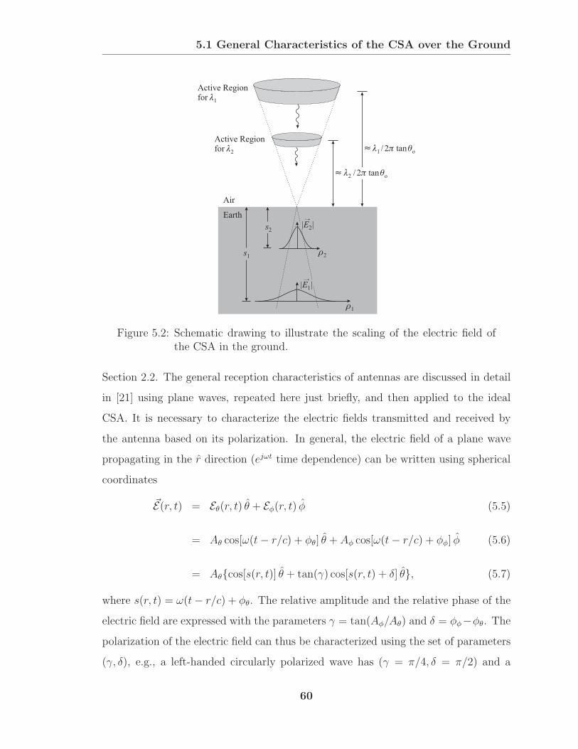
5.1 General Characteristics of the CSA over the Ground
2
1
Active Regionfor 1
Active Regionfor 2
Air
Earth
s2
s1
1 o/ 2 tan
2 o/ 2 tan
|E2|
|E1|
Figure 5.2: Schematic drawing to illustrate the scaling of the electric field ofthe CSA in the ground.
Section 2.2. The general reception characteristics of antennas are discussed in detail
in [21] using plane waves, repeated here just briefly, and then applied to the ideal
CSA. It is necessary to characterize the electric fields transmitted and received by
the antenna based on its polarization. In general, the electric field of a plane wave
propagating in the r direction (ejωt time dependence) can be written using spherical
coordinates
&E(r, t) = Eθ(r, t) θ + Eφ(r, t) φ (5.5)
= Aθ cos[ω(t− r/c) + φθ] θ + Aφ cos[ω(t− r/c) + φφ] φ (5.6)
= Aθcos[s(r, t)] θ + tan(γ) cos[s(r, t) + δ] θ, (5.7)
where s(r, t) = ω(t− r/c) + φθ. The relative amplitude and the relative phase of the
electric field are expressed with the parameters γ = tan(Aφ/Aθ) and δ = φφ−φθ. The
polarization of the electric field can thus be characterized using the set of parameters
(γ, δ), e.g., a left-handed circularly polarized wave has (γ = π/4, δ = π/2) and a
60

5.1 General Characteristics of the CSA over the Ground
right-handed circularly polarized wave has (γ = π/4, δ = −π/2). A straightforward
analysis shows that the ability of an antenna to receive a certain state of polarization
can be described using the polarization mismatch factor, pr, i.e.,
pr =1 + tan2(γtrans) tan
2(γrec)− 2 tan(γtrans) tan(γrec) cos(δtrans + δrec)
sec2(γtrans) sec2(γrec), (5.8)
where (γtrans, δtrans) characterizes the polarization of the electric field transmitted
by the antenna and (γrec, δrec) characterizes the polarization of the electric field being
received by the antenna. The mismatch factor varies between pr = 0 for null reception,
i.e., the electric field incident upon the antenna is not received at all, and pr = 1 for
maximum reception, i.e., the electric field incident upon the antenna is completely
received. The shape and orientation of the polarization ellipse, and the sense in which
the polarization ellipse is traced out (handedness) for null and maximum reception
are illustrated in Fig. 5.3 relative to the shape, orientation, and handedness of the
polarization ellipse for transmission. Figure 5.3a is for the most general case in which
the antenna transmits an elliptically polarized wave, while Fig. 5.3b is for a special
case in which the antenna transmits a left-handed circularly polarized wave. The
polarization ellipses on the left are for the electric field transmitted by the antenna
and plotted for an observer located beyond to antenna looking in the main radiation
direction. The polarization ellipses in the center (on the right) are for the electric field
with maximum (null) reception and plotted for an observer located at the antenna
looking in the direction of the wave incident upon the antenna; see Fig. 5.3c for the
position and orientation of the observers. Notice that for this choice of the coordinate
systems, the shape and handedness of the polarization ellipses do not change for
maximum reception, while the axis of the ellipse (orientation) is the mirror image
with respect to the φ axis relative to that for transmission. For null reception, the
shape remains the same, while the orientation of the ellipse changes by 90 relative
to that for maximum reception and the sense in which the polarization ellipse is
traced out reverses. The results presented in Fig. 5.3b can be directly applied to the
ideal left-handed CSA that radiates predominantly left-handed circular polarization
61
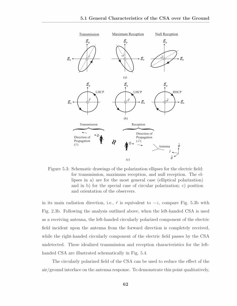
5.1 General Characteristics of the CSA over the Ground
Transmission Maximum Reception Null Reception
(a)
(b)
E
E
RHCP
E
E
-rE
E
LHCP
E
E
-r
-rE
E
LHCP
E
E
r
r
(c)
r
^
^
^
^
^
^
^
^
^Antenna
Direction ofPropagation( )r
Direction ofPropagation(- )r
Transmission Reception
-r
Figure 5.3: Schematic drawings of the polarization ellipses for the electric field:for transmission, maximum reception, and null reception. The el-lipses in a) are for the most general case (elliptical polarization)and in b) for the special case of circular polarization; c) positionand orientation of the observers.
in its main radiation direction, i.e., r is equivalent to −z, compare Fig. 5.3b with
Fig. 2.3b. Following the analysis outlined above, when the left-handed CSA is used
as a receiving antenna, the left-handed circularly polarized component of the electric
field incident upon the antenna from the forward direction is completely received,
while the right-handed circularly component of the electric field passes by the CSA
undetected. These idealized transmission and reception characteristics for the left-
handed CSA are illustrated schematically in Fig. 5.4.
The circularly polarized field of the CSA can be used to reduce the effect of the
air/ground interface on the antenna response. To demonstrate this point qualitatively,
62

5.1 General Characteristics of the CSA over the Ground
LHCP RHCP
Transmission Maximum Reception Null Reception
LHCP
Left-Handed CSA
RHCP
Figure 5.4: Idealized polarization characteristics of the left-handed CSA fortransmission and reception.
a simple plane-wave analysis based on the geometry shown in Fig. 5.5a is used. A
plane wave in free space with its electric field components parallel and perpendicular
to the plane of incidence, Einc‖ and Einc
⊥ , respectively, is incident upon the air/ground
interface with the angle αinc. The field is partially reflected into the free-space region
(µr = 1, εr = 1, σ = 0) and partially transmitted into the lossy medium (µrg =
1, εrg, σg). The reflected field components, Eref⊥ and Eref
‖ , can be written in terms of
the incident field components using the reflection coefficients for the corresponding
orientation (parallel and perpendicular to the plane of incidence), i.e., Eref⊥ = Γ⊥Einc
⊥
and Eref‖ = Γ‖Einc
‖ [24]. The results for the magnitude of the reflection coefficients
are graphed as a function of angle of incidence αinc in Figs. 5.5b and c for three soils:
dry, medium moist, and wet. The electrical parameters at the frequency f = 1.8GHz
(midband frequency of the CSA investigated in the next section) are given in Table
5.1 [25].
Table 5.1: Electrical parameters for different soil conditions at f = 1.8GHz.
εrg σg [S/m]
dry 4.0 0.02
medium 8.0 0.07
wet 15.0 0.15
63

5.1 General Characteristics of the CSA over the Ground
Earth rg g,
Free Space
kt
Et
Et
inc inc
Eref
Eref
krefEinc
Einc
kinc
(a)
(b)
(c)
0 10 20 30 40
0.00
0.25
0.50
0.75
1.00
0 10 20 30 40
0.00
0.25
0.50
0.75
1.00
inc
inc
DryMediumWet
Figure 5.5: a) Geometry of the plane-wave analysis. Analytical results for themagnitude of the reflection coefficient for the electric field b) par-allel to the plane of incidence and c) perpendicular to the plane ofincidence.
64
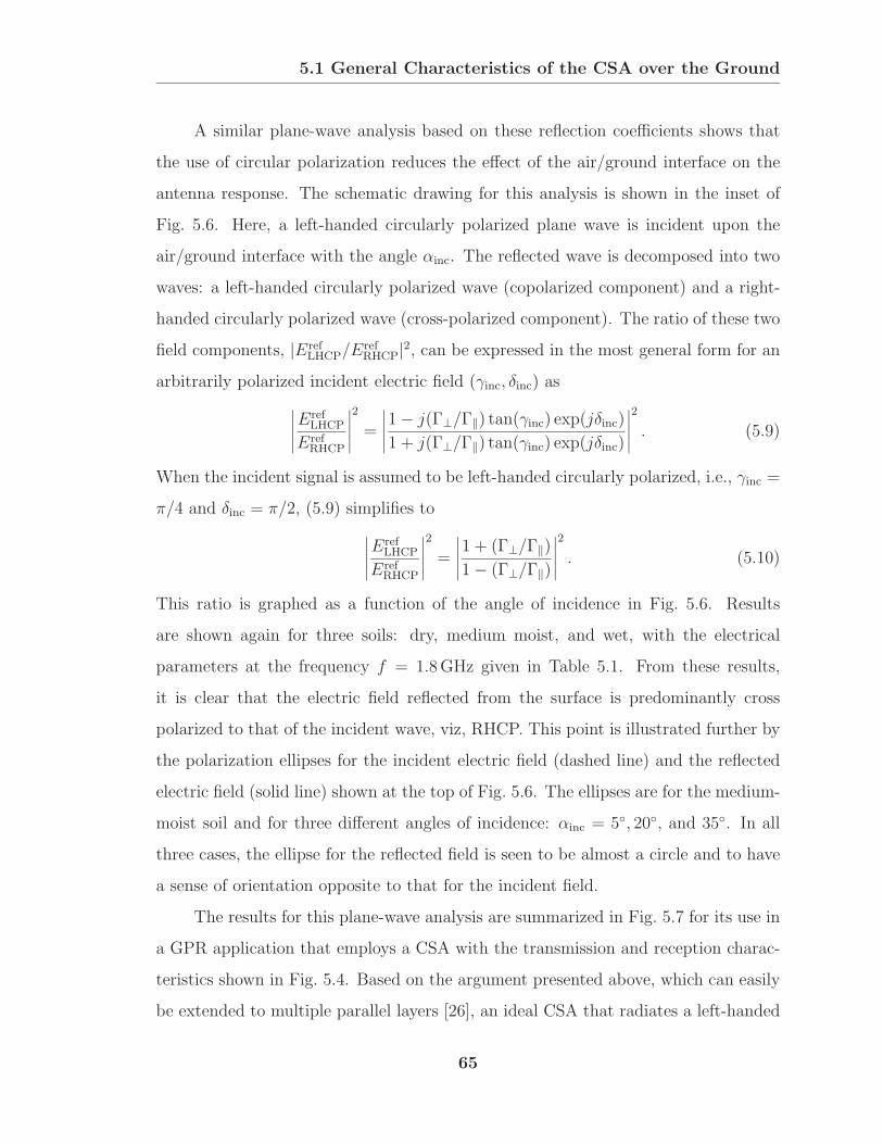
5.1 General Characteristics of the CSA over the Ground
A similar plane-wave analysis based on these reflection coefficients shows that
the use of circular polarization reduces the effect of the air/ground interface on the
antenna response. The schematic drawing for this analysis is shown in the inset of
Fig. 5.6. Here, a left-handed circularly polarized plane wave is incident upon the
air/ground interface with the angle αinc. The reflected wave is decomposed into two
waves: a left-handed circularly polarized wave (copolarized component) and a right-
handed circularly polarized wave (cross-polarized component). The ratio of these two
field components, |ErefLHCP/E
refRHCP|2, can be expressed in the most general form for an
arbitrarily polarized incident electric field (γinc, δinc) as∣∣∣∣∣ErefLHCP
ErefRHCP
∣∣∣∣∣2
=
∣∣∣∣∣1− j(Γ⊥/Γ‖) tan(γinc) exp(jδinc)1 + j(Γ⊥/Γ‖) tan(γinc) exp(jδinc)
∣∣∣∣∣2
. (5.9)
When the incident signal is assumed to be left-handed circularly polarized, i.e., γinc =
π/4 and δinc = π/2, (5.9) simplifies to
∣∣∣∣∣ErefLHCP
ErefRHCP
∣∣∣∣∣2
=
∣∣∣∣∣1 + (Γ⊥/Γ‖)1− (Γ⊥/Γ‖)
∣∣∣∣∣2
. (5.10)
This ratio is graphed as a function of the angle of incidence in Fig. 5.6. Results
are shown again for three soils: dry, medium moist, and wet, with the electrical
parameters at the frequency f = 1.8GHz given in Table 5.1. From these results,
it is clear that the electric field reflected from the surface is predominantly cross
polarized to that of the incident wave, viz, RHCP. This point is illustrated further by
the polarization ellipses for the incident electric field (dashed line) and the reflected
electric field (solid line) shown at the top of Fig. 5.6. The ellipses are for the medium-
moist soil and for three different angles of incidence: αinc = 5, 20, and 35. In all
three cases, the ellipse for the reflected field is seen to be almost a circle and to have
a sense of orientation opposite to that for the incident field.
The results for this plane-wave analysis are summarized in Fig. 5.7 for its use in
a GPR application that employs a CSA with the transmission and reception charac-
teristics shown in Fig. 5.4. Based on the argument presented above, which can easily
be extended to multiple parallel layers [26], an ideal CSA that radiates a left-handed
65

5.2 Numerical Analysis of the CSA over the Ground
inc = 35oinc = 5
o inc = 20o
0 10 20 30 400.000
0.025
0.050
0.075
inc
Earth
Free Space
inc inc
ELHCPELHCP
ERHCPinc
ref
ref
EL
HC
P
ref
ER
HC
P
ref
/2
DryMediumWet
ReflectedIncident
Figure 5.6: Analytical results for the ratio |ErefLHCP/E
refRHCP|2 as a function of
angle of incidence αinc for three different types of soil. Polarizationellipses for the incident and reflected electric fields are shown forthe medium-moist soil.
circularly polarized wave toward the air/ground interface does not receive the wave
reflected from any media interface, because it is predominantly right-handed circu-
larly polarized.1 This feature can be useful in applications, such as GPRs, where
a signal from within the ground is to be measured, not a signal reflected from the
surface of the ground, which is considered to be “clutter.”
5.2 Numerical Analysis of the CSA over the Ground
In this section, an accurate analysis of the CSA over the ground is performed using
the FDTD method, and results obtained from this analysis are used to verify and
1Precisely, this is correct only for media interfaces of two parallel, isotropic media infinite in ex-
tent. It will be shown in Section 5.4 that an anisotropic medium can scatter a significant copolarized
signal.
66

5.2 Numerical Analysis of the CSA over the Ground
RHCP
LHCP
Earth
LHCP
RHCP
Left-handed CSA
Layer
Figure 5.7: Schematic drawing to illustrate that the use of circular polariza-tion reduces the effect of the air/ground interface on the antennaresponse.
quantify the characteristics of the CSA that are discussed qualitatively in the last
section. The FDTD technique has been applied to the CSA in free space in Chapter 2,
and numerical results for the input impedance and realized gain are in good agreement
with measurements, see Section 2.2. Thus, the same techniques can be applied to a
similar CSA over the ground with confidence.
The two-arm CSA has the geometry shown in Fig. 2.1 with the following pa-
rameters: θ = 7.5, α = 75, δ = 90, and D/d = 8 (d = 2 cm). The antenna
is fed from a transmission line with the characteristic impedance Zc = 100Ω. To
improve the low-frequency performance, the CSA is terminated with a resistive sheet
to reduce the reflections from the open end, see Chapter 4. The electrical and ge-
ometrical parameters of the sheet are chosen to make the DC resistance, measured
between the two arms, 150Ω.2 When this antenna is isolated in free space, it has an
operational (hybrid) bandwidth of about 6.3, extending from 0.49GHz to 3.1GHz,
see Chapter 3. For all of the results to be presented, the virtual apex of the CSA
is placed at the air/ground interface, so the height h of the drive point above the
2Recall, this is the most practical choice for the characteristic impedance of the line and for the
load resistance, see Section 4.1 and Fig. 3.5.
67
5.2 Numerical Analysis of the CSA over the Ground
RX
,[
]
f [GHz]
0.25 0.50 1.00 1.50 2.00 2.50 3.00 3.50
-25
0
25
50
75
100
125
150
175
R
X
j2
j1
j0.5
j0.2
0
- 0.2j
- 0.5j- 1j
- 2j
1 2 50.50.2
R Z/ c
X Z/ c
Free SpaceOver Ground
Operational Bandwidth
Figure 5.8: Comparison of the input impedances for the CSA in free space andover medium-moist soil.
ground is h = 7.6 cm.
The input impedances of the CSA when isolated in free space (solid line) and
when placed over the medium-moist soil (dashed line) are compared in Fig. 5.8. The
presence of the ground is seen to have almost no effect on the input impedance, and
both the resistance and reactance are seen to be nearly frequency independent over the
operational bandwidth of the antenna. Notice that the reactance is small compared
to the resistance, and that the resistance is approximately R ≈ 140Ω. Thus, over
the operational bandwidth, the antenna is well matched to the feeding transmission
line (Zc = 100Ω). This is clearly shown on the Smith chart that is inset in Fig. 5.8.
Similar results are obtained for the other two soil conditions: dry and wet. So for this
arrangement, the input impedance of the CSA is essentially independent of frequency
and independent of the electrical properties of the ground.
The effect of the ground on the time-domain results for the antenna response
is qualitatively shown in Fig. 5.9. In Fig. 5.9a, the reflected voltage for the CSA
over the ground, Vref,g, is graphed as a function of normalized time, t/τL, with thecharacteristic time of the incident, differentiated Gaussian pulse, τp/τL = 1.3 · 10−2.Other than the drive-point reflection at t/τL ≈ 0 and the antenna-end reflection at
68

5.2 Numerical Analysis of the CSA over the Ground
-0.5 0.0 1.0 2.0 3.0 4.0
-0.2
-0.1
0.0
0.1
0.2
t / L
Vre
f,g
/V
o
(a)
-0.5 0.0 1.0 2.0 3.0 4.0
-0.010
-0.005
0.000
0.005
0.010
t / L
Vsc
att
,g
/V
o
(b)
Figure 5.9: Theoretical results for a) the reflected voltage of the CSA overground and b) the voltage of the signal scattered from theair/ground interface.
t/τL ≈ 2, no additional reflected signals, e.g., from the ground, are obvious. The
effect of the air/ground interface can be quantified when the reflected voltage of the
CSA over the ground, Vref,g, is subtracted from the voltage of the CSA in free space,
Vref,fs, i.e., the voltage of the signal scattered from the air/ground interface can be
written Vscatt,g = Vref,fs − Vref,g. This voltage is shown in Fig. 5.9b; as expected, thisvoltage is very small.
Two factors contribute to the observed behavior for the input impedance and
the reflected voltage of the CSA over the ground. The lack of a major effect due to
the presence of the ground is a result of the CSA not receiving the signal reflected
from the ground. The frequency independence is a result of the angle principle and
69

5.2 Numerical Analysis of the CSA over the Ground
the truncation principle being satisfied to the same degree for the CSA isolated in
free space and for the CSA with its virtual apex at the air/ground interface.
Figure 5.10 shows the characteristics of the electric field along the z axis (axis
of the CSA) in the ground. The graph in Fig. 5.10a verifies the scaling of the electric
field given by (5.4). It shows the normalized electric field as a function of the depth
in the ground. For the plot, depths in the range 0.2m ≤ s ≤ 1m are used, and
at each depth, the free-space wavelength at which the electric field is evaluated is
set equal to 0.6 times the depth; that is, s/λ = const = 1.67, which satisfies (5.3).
Results are shown for free space (εrg = 1.0, σg = 0, solid line), for the medium-moist
soil with loss (εrg = 8.0, σg = 0.07 S/m, dashed line) and for the medium-moist soil
without loss (εrg = 8.0, σg = 0, dash-dotted line). Notice that the exponential factor
exp(αs), where α ≈ σgη/2√εrg is the attenuation constant in the soil, is included in
the normalization to remove the effect of the attenuation in the lossy ground. The
curves are seen to be nearly the same and to be almost uniform. This verifies the
scaling of the electric field described by (5.4).
The graph in Fig. 5.10b shows the axial ratio for the polarization ellipse of the
electric field versus frequency for two very different depths in the medium-moist soil
(s = 4 cm, dashed line; and s = 1m, dash-dotted line). Here, the axial ratio, usually
a far-field quantity, is determined in the near zone of the CSA using the electric field
components normal to the axis of the antenna, Ex and Ey. At the depths used, the
component of the electric field parallel to this axis, Ez, is orders of magnitude smaller
than those normal to the axis. As a point of reference, the axial ratio for the electric
field at the apex of the antenna when isolated in free space is also shown (solid line).
Recall, for circular polarization, the axial ratio is AR = 1.0. The electric field in
the ground is seen to be nearly circularly polarized over the operational bandwidth
of the antenna (AR ≤ 1.25, for 0.49GHz ≤ f ≤ 3.1GHz) and to be similar to that
for the isolated antenna. This point is further illustrated by plots of the polarization
ellipse at the top of the figure. They are for the electric field at the depth s = 1m
(solid line) in the medium-moist soil and for circular polarization (dotted line) at the
70

5.2 Numerical Analysis of the CSA over the Ground
(a)
()
|| /
||
exp(
)E
Vs
inc
s [m]
0.2 0.4 0.6 0.8 1.0
0.00
0.25
0.50
0.75
1.00
1.25
Free SpaceLossy GroundLossless Ground
(b)
0.25 0.50 1.00 1.50 2.00 2.50 3.00 3.50
1.00
1.25
1.50
1.75
2.00 Free Space (at Apex)Ground ( =4cm)Ground (Circ. Polarization
ss =1m)
f [GHz]
AR
Figure 5.10: a) Theoretical results for the normalized electric field on axis as afunction of depth: in free space (solid line), in the lossy, medium-moist soil (dashed line), and in the lossless medium-moist soil (dash-dotted line). b) Theoretical results for the axial ratio on axis forthe CSA in free space at the apex (solid line), for the CSA overthe medium-moist soil observed 4 cm (dashed line), and 1m (dash-dotted line) below the air/ground interface.
frequencies f = 0.50, 1.75, and 3.00GHz.
In some applications, such as GPRs used to detect landmines buried in the
ground or reinforcing bars embedded in concrete, the characteristics of the electric
field at a shallow depth in the ground are of interest. At such depths, the distance
from the buried object to the virtual apex of the CSA is small. So the characteristics
71
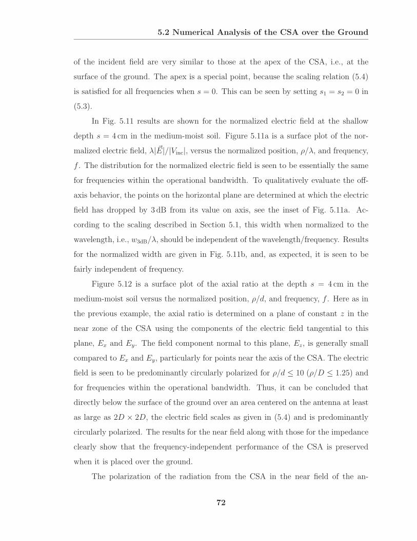
5.2 Numerical Analysis of the CSA over the Ground
of the incident field are very similar to those at the apex of the CSA, i.e., at the
surface of the ground. The apex is a special point, because the scaling relation (5.4)
is satisfied for all frequencies when s = 0. This can be seen by setting s1 = s2 = 0 in
(5.3).
In Fig. 5.11 results are shown for the normalized electric field at the shallow
depth s = 4 cm in the medium-moist soil. Figure 5.11a is a surface plot of the nor-
malized electric field, λ| &E|/|Vinc|, versus the normalized position, ρ/λ, and frequency,f . The distribution for the normalized electric field is seen to be essentially the same
for frequencies within the operational bandwidth. To qualitatively evaluate the off-
axis behavior, the points on the horizontal plane are determined at which the electric
field has dropped by 3 dB from its value on axis, see the inset of Fig. 5.11a. Ac-
cording to the scaling described in Section 5.1, this width when normalized to the
wavelength, i.e., w3dB/λ, should be independent of the wavelength/frequency. Results
for the normalized width are given in Fig. 5.11b, and, as expected, it is seen to be
fairly independent of frequency.
Figure 5.12 is a surface plot of the axial ratio at the depth s = 4 cm in the
medium-moist soil versus the normalized position, ρ/d, and frequency, f . Here as in
the previous example, the axial ratio is determined on a plane of constant z in the
near zone of the CSA using the components of the electric field tangential to this
plane, Ex and Ey. The field component normal to this plane, Ez, is generally small
compared to Ex and Ey, particularly for points near the axis of the CSA. The electric
field is seen to be predominantly circularly polarized for ρ/d ≤ 10 (ρ/D ≤ 1.25) and
for frequencies within the operational bandwidth. Thus, it can be concluded that
directly below the surface of the ground over an area centered on the antenna at least
as large as 2D × 2D, the electric field scales as given in (5.4) and is predominantlycircularly polarized. The results for the near field along with those for the impedance
clearly show that the frequency-independent performance of the CSA is preserved
when it is placed over the ground.
The polarization of the radiation from the CSA in the near field of the an-
72

5.2 Numerical Analysis of the CSA over the Ground
f [GHz]
w3
dB
/
0.3 0.5 1.0 1.5 2.0 2.5 3.0 3.5
0.0
0.5
1.0
1.5
2.0
Free Space (at Apex)Ground ( =4cm)s
|
| /|
| [d
B]
EV
inc
/f [GHz]
(a)
(b)
|E |norm
w3dB
0.51.0
1.52.0
2.53.0
3.5
Figure 5.11: a) The normalized electric field distribution 4 cm below theair/ground interface as a function of frequency and distance fromthe axis. b) Results for the normalized 3 dB width as a function offrequency for the antenna in free space observed at the apex (solidline) and for the antenna over the medium-moist ground observedat 4 cm below the apex (dashed line).
tenna and the scattering characteristics from the air/ground interface are studied
qualitatively using the electric field in the vicinity of the antenna. In Fig. 5.13a, the
normalized, left-handed and right-handed circularly polarized field components of the
incident electric field, Einc,n = |Einc/(VincLs)|, are plotted as a function of frequencyfor the CSA in free space. For clarity, these fields, ELHCP
inc,n and ERHCPinc,n , are normalized
by the maximum value of the LHCP component, ELHCP,maxinc,n . The electric field is
observed on axis and 0.5 cm above the virtual apex of the antenna. Similar to the
73
5.2 Numerical Analysis of the CSA over the Ground
/df [GHz]
AR
2.0
1.8
1.6
1.4
1.2
1.0
0.51.0
1.52.0
2.53.0
3.5
Figure 5.12: The axial ratio at a depth of 4 cm below the air/ground interfaceas a function of frequency and distance from the axis.
electric field in the far field of the antenna, the polarization of the electric field in the
near field of the antenna is predominantly left handed. Recall that the air/ground in-
terface predominantly scatters the cross-polarized component of the incident electric
field. For normal incidence, the reflection coefficients for the electric field perpendicu-
lar and parallel to the plane of incidence, are the same, i.e., Γ = Γ⊥ = Γ‖ for αinc = 0.
For this case, the ratio of the cross-polarized component of the electric field scattered
from the air/ground interface to the corresponding component of the incident electric
field must equal the reflection coefficient, i.e., ERHCPref /ELHCP
inc = ELHCPref /ERHCP
inc = Γ.
This behavior is verified in Fig. 5.13b for the ratio ERHCPref /ELHCP
inc as a function of
frequency. The reflected/scattered electric field (on axis 0.5 cm above the apex) is
obtained by subtracting the electric field for the CSA over the ground, &Eground, from
the electric field component of the CSA in free space, &Einc, i.e., Eref = | &Eground− &Einc|.This ratio is graphed for three different soils: dry (solid line), medium moist (dashed
line), and wet (dash-dotted line), and the corresponding reflection coefficients are
graphed with dotted lines. Since the ratio of the electric fields matches the value for
the reflection coefficient well over the entire frequency range, the scattering from the
air/ground interface can be correctly described by the plane-wave analyses in Section
74

5.3 GPR Applications
0.5 1.0 1.5 2.0 2.5 3.0 3.5 4.0
0.00
0.25
0.50
0.75
1.00
1.25
0.5 1.0 1.5 2.0 2.5 3.0 3.5 4.0
0.00
0.25
0.50
0.75
1.00
f [GHz]
(a)
||
EE
/in
c,
inc,
nn
LH
CP,
max
f [GHz]
(b)
LH
CP
|Ere
f/
Ein
c|
RH
CP
DryMediumWet
LHCPRHCP
wet
medium
dry
Figure 5.13: Theoretical results for a) the electric field of the CSA in free spacein the near field of the antenna and b) the electric field scatteredfrom the air/ground interface.
5.1. Similar agreement can be obtained for the results for the ratio of ELHCPref /ERHCP
inc ,
which are omitted since this reflected component of the electric field is very small. In
conclusion, this simple analysis confirms and quantifies that the air/ground interface
predominantly reflects the cross-polarized component of the incident electric field.
5.3 GPR Applications
In the following, monostatic GPRs are investigated that use a single two-arm CSA
for transmission and reception. Different objects buried in the ground are used to
75

5.3 GPR Applications
RHCPLHCP
Earth
LHCP
LPLHCP
Thin Rod
+
Left-handed CSA
Lr
sr
h
Figure 5.14: Schematic drawing for a monostatic GPR that uses a single CSAto detect thin metallic rods buried in the ground.
illustrate the sensitivity of the CSA to the polarization of the scattered electric field
of the target. In the first case, the targets are thin metallic rods that predominantly
scatter linear polarization, while in the second case, the targets are buried plastic
mines.
5.3.1 GPR: Detection of Buried Rods
Here, a monostatic GPR is investigated for detecting thin metallic rods buried in the
ground. Figure 5.14 is a schematic drawing for this GPR that uses a left-handed,
two-arm CSA. A rod of length Lr buried at the depth sr in the ground predomi-
nantly scatters linear polarization, which can be decomposed into equal left-handed
and right-handed circularly polarized components. Ideally, only the copolarized com-
ponent (LHCP) can be received by this CSA and used to detect the rod buried in
the ground. It will be shown that the rod buried in the ground with electrical pa-
rameters µrg = 1, εrg, and σg can be detected at the resonant frequencies of the
76
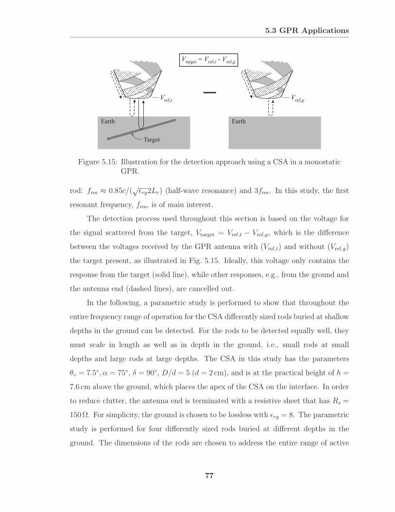
5.3 GPR Applications
Earth
Target
Vref,t
Earth
Vref,g
V V Vtarget ref, ref,= -t g
Figure 5.15: Illustration for the detection approach using a CSA in a monostaticGPR.
rod: fres ≈ 0.85c/(√εrg2Lr) (half-wave resonance) and 3fres. In this study, the first
resonant frequency, fres, is of main interest.
The detection process used throughout this section is based on the voltage for
the signal scattered from the target, Vtarget = Vref,t − Vref,g, which is the difference
between the voltages received by the GPR antenna with (Vref,t) and without (Vref,g)
the target present, as illustrated in Fig. 5.15. Ideally, this voltage only contains the
response from the target (solid line), while other responses, e.g., from the ground and
the antenna end (dashed lines), are cancelled out.
In the following, a parametric study is performed to show that throughout the
entire frequency range of operation for the CSA differently sized rods buried at shallow
depths in the ground can be detected. For the rods to be detected equally well, they
must scale in length as well as in depth in the ground, i.e., small rods at small
depths and large rods at large depths. The CSA in this study has the parameters
θ = 7.5, α = 75, δ = 90, D/d = 5 (d = 2 cm), and is at the practical height of h =
7.6 cm above the ground, which places the apex of the CSA on the interface. In order
to reduce clutter, the antenna end is terminated with a resistive sheet that has Rs =
150Ω. For simplicity, the ground is chosen to be lossless with εrg = 8. The parametric
study is performed for four differently sized rods buried at different depths in the
ground. The dimensions of the rods are chosen to address the entire range of active
77
5.3 GPR Applications
regions along the antenna, as illustrated in Fig. 5.16a. Notice that four active regions
are indicated on the CSA (numbered 1, . . . , 4), and that each active region is for
the resonant frequency of the corresponding rod. In the simplest approximation, the
resonant frequency (half-wave resonance) of the buried rod matches the characteristic
frequency of the active region. The range of frequencies over which the antenna can
be operated ranges approximately from 0.78GHz to 3.1GHz. Thus, the lengths of
the rods are chosen to illustrate the uniform performance over this bandwidth. The
longest rod has Lr1 = 5.0 cm and fres1 ≈ 0.9GHz; the others have Lri = Lr1/i and
fresi = ifres1, where i = 1, . . . , 4. The burial depth in the ground is chosen to be
sr ≈ 0.7Lr, and thus scales with the length of the rod.
The results from the parametric study for the CSA are shown in Fig. 5.17a;
the normalized voltage for the signal scattered from the rods, |V rodtarget/Vinc| is shown
as a function of frequency. From these results, it can be seen that the large rods
are detected at low frequencies and the small rods at high frequencies. As mentioned
earlier, the level of detection should ideally be the same for rods when properly scaled
in length and depth; however, the received signals scattered from the smaller rods
(detection at high frequencies) are somewhat smaller than those for the larger rods.
This is probably due to reduced radiation at higher frequencies; in the far field this
is evident in the realized gain, see Fig. 4.11a, which trails off at the high end of the
frequency range.
To demonstrate the efficiency of the CSA in a GPR for detecting buried rods, a
similar study was performed for a GPR that uses a series of resonant dipole antennas
to detect the buried rods, Fig. 5.16b. To minimize the polarization loss, the dipole
antennas are aligned with the rods. The length of each of the dipoles is chosen so
that the dipole is resonant: Ldip ≈ 3.3Lr ≈ √εrgLr. The height of each dipole above
the ground is hdip ≈ 2.2Ldip and thus is approximately the same as the height of the
active region of the CSA. Results from this study are shown in Fig. 5.17b. Notice
that the signals received by each dipole peaks at roughly the resonant frequency of
the rod and that the level of detection is almost the same for all of the dipoles, as
78
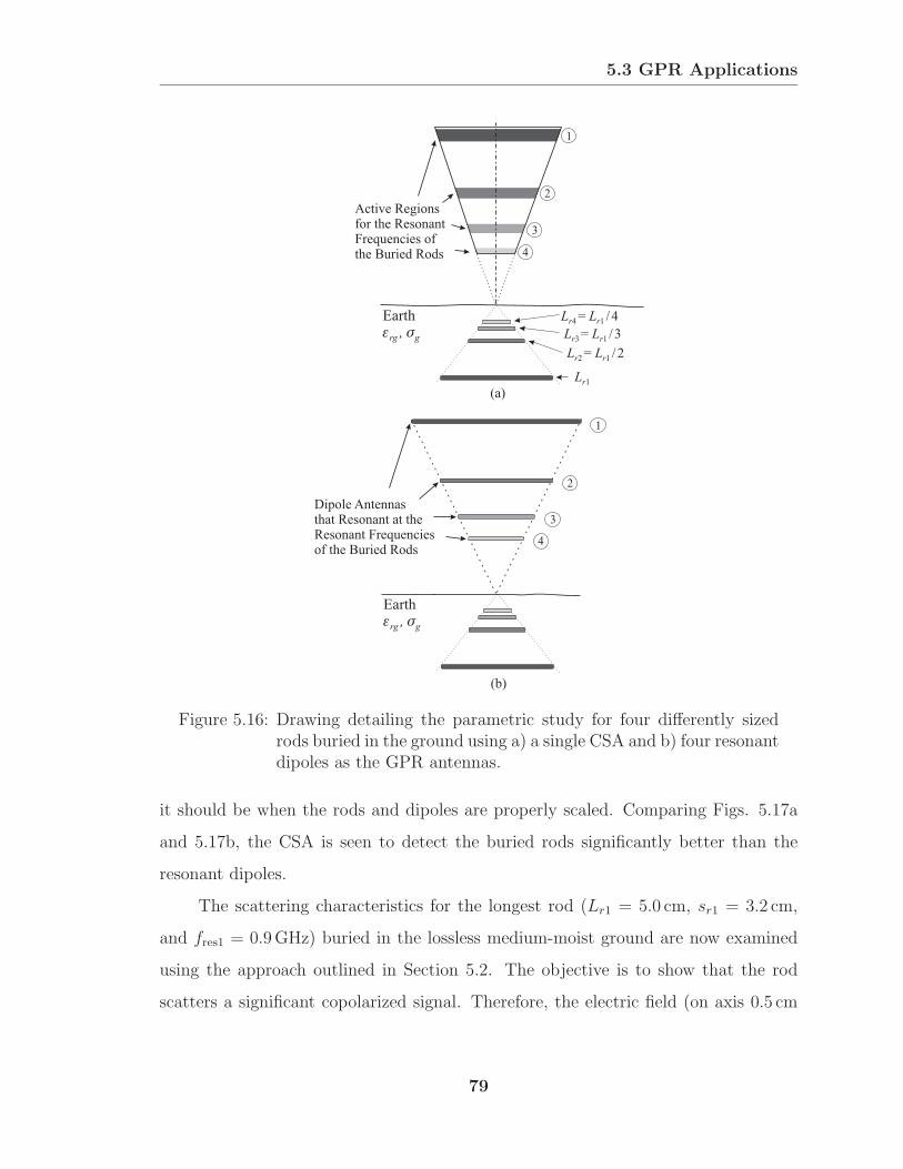
5.3 GPR Applications
Earth rg g,
Earth rg g,
L Lr r4 1= /4
L Lr r3 1= /3
L Lr r2 1= /2
Lr1
Active Regionsfor the ResonantFrequencies ofthe Buried Rods
Dipole Antennasthat Resonant at theResonant Frequenciesof the Buried Rods
1
1
2
2
3
3
4
4
(a)
(b)
Figure 5.16: Drawing detailing the parametric study for four differently sizedrods buried in the ground using a) a single CSA and b) four resonantdipoles as the GPR antennas.
it should be when the rods and dipoles are properly scaled. Comparing Figs. 5.17a
and 5.17b, the CSA is seen to detect the buried rods significantly better than the
resonant dipoles.
The scattering characteristics for the longest rod (Lr1 = 5.0 cm, sr1 = 3.2 cm,
and fres1 = 0.9GHz) buried in the lossless medium-moist ground are now examined
using the approach outlined in Section 5.2. The objective is to show that the rod
scatters a significant copolarized signal. Therefore, the electric field (on axis 0.5 cm
79

5.3 GPR Applications
1 2 3 4
1 2 3 4
1.0
1.0
0.5
0.5
2.0
2.0
3.0
3.0
4.0
4.0
0.000
0.004
0.008
0.012
0.000
0.004
0.008
0.012
f [GHz]
f [GHz]
(a)
(b)
|/
|V
Vta
rget
inc
rod
|/
|V
Vta
rget
inc
rod
Figure 5.17: Theoretical results for the parametric study for a) the monostaticGPR using a single CSA and b) a series of resonant dipoles to detectthin metallic rods buried in the ground.
above the apex) scattered from the rod is obtained by subtracting the electric field for
the CSA over the ground with the rod present, &Erod, from the electric field component
of the CSA over the ground without the rod, &Eground, i.e., Eref, rod = | &Erod − &Eground|.This electric field, normalized by the LHCP component of the incident electric field
ELHCPinc (obtained from the CSA in free space) is graphed in Fig. 5.18 as a function of
frequency. The rod is seen to scatter linear polarization because the right-handed and
left-handed circularly polarized components of the scattered electric field are equal.
As noted earlier, the rod scatters predominantly at the resonant frequencies, fres and
3fres.
80

5.3 GPR Applications
0.5 1.0 1.5 2.0 2.5 3.0 3.5 4.0
0.0
0.1
0.2
0.3
f [GHz]
LH
CP
||
Ere
f,ro
d/
Ein
c
LHCPRHCP
LHCP RHCP
Figure 5.18: Theoretical results for the electric field scattered from the rodburied in the ground.
To conclude the discussion of the GPR application to detect buried rods in the
ground, another parametric study is performed using rods buried in lossy ground
and at larger depths. In order to achieve good penetration of the electric field into
the ground, the operational frequency range for the monostatic radar is chosen to be
0.16GHz ≤ f ≤ 1.0GHz [25, 27]. The ground is dry soil, which has the following
electrical properties within this bandwidth: εrg ≈ 4 and σg ≈ 0.007 S/m.3 The left-
handed CSA has the dimensions θ = 7.5, α = 75, δ = 90, D/d = 8 (d = 6 cm)
and is placed at a height of h = 22.8 cm over the ground. Notice that this is a scaled
version of the CSA discussed earlier in Section 5.2: all of the dimensions are three
times larger and the operational bandwidth is lower in frequency by a factor of three.
As in the previous case, the CSA is terminated with a resistive sheet (Rs = 150Ω).
The lengths of the five rods used in the parametric study are chosen to illustrate
the uniform performance of the radar over the operational bandwidth. For the longest
rod Lr1 = 32 cm, and fres1 ≈ 0.2GHz; and for the other rods Lri = Lr1/i and fres i ≈ifres1, i = 2, . . . , 5. The rods are buried at depths such that sri/Lri = const = 3.1,
3Notice that this conductivity is lower than the value given for dry soil in Table 5.1. This is caused
by the difference in the frequency: The value in Table 5.1 is for the frequency f = 1.8GHz, while
the value used in the present calculation is for the center frequency of the operational bandwidth,
f = 0.6GHz.
81

5.3 GPR Applications
0.15 0.30 0.45 0.60 0.75 0.90 1.05 1.200.000
0.002
0.004
0.006
0.008
0.010
f [GHz]
1 2 3 4 5
|VV
sta
rget
inc
/| e
xp
(2)
r
rod
Figure 5.19: Results for the monostatic GPR with the thin rods buried in thedry soil.
so for the longest rod, the depth is sr1 = 1m, and for the shortest rod, the depth is
sr5 = 0.2m.
In Fig. 5.19, the voltage |V rodtarget/Vinc| exp(2αsr) is plotted versus frequency. The
factor exp(2αsr) accounts for the attenuation of the waves propagating the round-
trip distance 2sr (to and from the rod) in the ground. Notice that there is a peak
at the resonant frequency of each rod, and that all of the peaks have comparable
amplitudes. These results show that the monostatic radar based on the CSA is
equally good for detecting small targets at shallow depths and large targets at large
depths. The overall conclusion that can be drawn from these parametric studies is
that a monostatic radar that uses a single CSA can detect buried rods, because the
rods scatter a significant copolarized signal.
5.3.2 GPR: Detection of Buried Mines
In this section, a monostatic GPR is investigated for detecting plastic landmines
buried in the ground. The model for this GPR is shown schematically in Fig. 5.20a.
Recall for an ideal CSA, the detection of buried mines must be based on the reception
of the copolarized components of the field scattered from the mine. The ideal CSA
should not detect a mine that is concentric with the antenna (the axis of the mine
82

5.3 GPR Applications
RHCPLHCPLHCP
EarthLHCP
+
Left-handed CSA
Mine
(a)
Mine
DM
sMdM
h
hM
Earth rg g,
rM
(b)
Figure 5.20: a) Schematic drawing for the monostatic GPR used to detect buriedplastic mines, b) parameters that describe the mine and the relativepositioning of the antenna and the mine.
aligned with the axis of the CSA). The detection of the mine must therefore be based
on the copolarized component of the scattered field produced when the antenna and
mine are not concentric, i.e., for detection the scattering from the edges of the mine
should produce a sufficient copolarized signal, see Fig. 5.20a
A parametric study was performed to study the performance of the radar to
detect differently sized mines buried at different depths in the ground. The antenna
parameters were chosen to be θ = 7.5, α = 75, δ = 90, D/d = 5 (d = 2 cm), and
83

5.3 GPR Applications
h = 7.6 cm. The CSA was terminated at the big end with a resistive sheet that has
Rs = 150Ω. The ground with a relative permittivity εrg = 8 was modeled both as a
lossless medium (σg = 0) and as a lossy medium, in which case the conductivity at
the midband frequency (f = 1.8GHz) was σg = 0.07 S/m. In this parametric study,
three differently sized mines were used, the details of the mine are shown in Fig. 5.20b.
The mines were lossless with relative permittivity εrM = 3, which corresponds to the
electrical properties of commonly used explosives, and their diameters were DM =
9.0 cm, 13.5 cm, and 18.0 cm. The sizes of these mines range from antipersonnel to
antitank mines. The height of the mine hM and the depth in the ground dM (measured
between the top of the mine and the air/ground interface) were scaled to the diameter
of the mine, i.e., hM ≈ DM/2 and dM ≈ DM/2. Two lateral positions of the axis
of the CSA relative to the mine were considered: the CSA centered over the mine
(sM = 0) and the CSA centered over the edge of the mine (sM = DM/2).
The results from the parametric study are shown in Fig. 5.21. The voltage for
the signal scattered from the mine, V minetarget, is plotted as a function of frequency for
the biggest mine (DM = 18 cm) in Fig. 5.21a, for the medium-sized mine (DM =
13.5 cm) in Fig. 5.21b, and for the smallest mine (DM = 9 cm) in Fig. 5.21c. For
clarity, the results from this study are plotted after post processing. A straightforward
(smoothing) filter was applied to the raw data in order to reduce high-frequency
ripples on the results. In these plots, the black curves correspond to the lossless ground
while the gray curves correspond to the lossy ground. The two shifts considered in this
study are shown with different linestyles, the solid curve is for the CSA centered over
the mine and the dashed curve is for the CSA centered over the edge of the mine. The
scattering from the biggest mine can be seen throughout the frequency range, while
scattering from the smallest mine can only be seen at the higher frequencies. When
the ground is lossy, the attenuation causes the signal to decrease over the entire range
of frequencies (compare black and gray lines). Contrary to the previous expectations,
the effect of the mine, i.e., the scattered signal received by the CSA, is biggest when
the antenna is concentric with the mine, and not when it is centered over the edge of
84

5.3 GPR Applications
Lossless Ground
Lossy Ground
Centered over MineCentered over Edge
0.000
0.000
0.000
0.004
0.004
0.004
0.008
0.008
0.008
0.012
0.012
0.012
1 2 3 4
f [GHz]
(a)
0.5
1 2 3 4
f [GHz]
(c)
0.5
1 2 3 4
f [GHz]
(b)
0.5
||
VV
targ
et
inc
/m
ine
||
VV
targ
et
inc
/m
ine
||
VV
targ
et
inc
/m
ine
Figure 5.21: Theoretical results for the parametric study for the monostaticGPR using a single CSA to detect buried plastic mines: a) DM =18 cm, b) DM = 13.5 cm, and c) DM = 9 cm.
85

5.4 Removing the Dispersion in the CSA
the mine. This result must be caused by the imperfections in the antenna that allow
it to receive the cross-polarized component of the scattered signal. The conclusion
that can be drawn from this parametric study is that a monostatic radar that uses
a single CSA can only marginally detect buried plastic mines. The reason for this is
that the plastic mines do not scatter a sufficient amount of copolarized signal. This
is true even when the CSA is centered over the edge of the mine.
The scattering characteristics of the mine in the lossless ground are examined in
the same manner as in the previous GPR application, Section 5.3.1, to confirm that
the mine does not scatter a significant copolarized signal. The electric field (on axis
0.5 cm above the apex) scattered from the smallest mine (DM = 9 cm) is obtained
by subtracting the electric field for the CSA over the ground with the mine present,
&Emine, from the electric field component of the CSA over the ground without the mine,
&Eground, i.e., Eref,mine = | &Emine− &Eground|. This electric field, normalized by the LHCPcomponent of the incident electric field ELHCP
inc (obtained from the CSA in free space)
is graphed for the mine on axis in Fig. 5.22a, and for the mine off axis in Fig. 5.22b.
From these graphs, it is clear that the copolarized signal scattered from the mine is
too small for the monostatic GPR to clearly detect the mine buried in the ground.
5.4 Removing the Dispersion in the CSA
This section is concerned with CSAs that are used in radars that radiate and receive
short pulses. Specifically, a practical approach will be described for removing the
dispersion introduced by the CSA. Upon transmission and reception from the CSA,
signals disperse due to the movement of the active region with frequency. This dis-
persion is undesired, e.g., when CSAs are used in radars, since the received signals
are spread out in time and not clearly distinguishable from other reflections, e.g., the
antenna end reflection and the reflection from the target. A straightforward and also
practical approach is introduced which removes the dispersion from the response; this
increases the chances for successful detection.
86

5.4 Removing the Dispersion in the CSA
(b)
0.5 1.0 1.5 2.0 2.5 3.0 3.5 4.0
0.0
0.1
0.2
0.3
0.4
f [GHz]
LH
CP
Ere
f,m
ine
/E
inc
0.5 1.0 1.5 2.0 2.5 3.0 3.5 4.0
0.0
0.1
0.2
0.3
0.4
f [GHz]
LH
CP
Ere
f,m
ine
/E
inc
(a)
LHCPRHCP
Figure 5.22: Theoretical results for the electric field scattered from the buriedmine: a) on axis and b) off axis.
The radar investigated uses a CSA in free space with the geometry θ = 7.5,
α = 75, δ = 90, and D/d = 8 (d = 2 cm). To reduce clutter, the CSA is terminated
at the big end using a resistive sheet (Rs = 150Ω). A perfectly conducting pipe of
square cross section with equal height and width of w = 15 cm and of infinite length4
is displaced from the apex of the cone by s = 1m (measured from the apex to the top
of the pipe), see Fig. 5.23. The conventional algorithm used to obtain the signature
of the target is outlined in Fig. 5.15 and based on the spectrum of the signal scattered
from the target. This voltage is the basis for another approach; however, instead of
using the voltage in the frequency domain, the main interest is now the voltage in
4In the FDTD, this infinitely long pipe is modeled by extending the pipe into the PML.
87
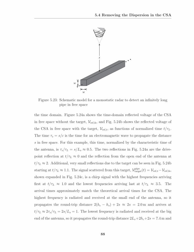
5.4 Removing the Dispersion in the CSA
s
w
w
…
…
Figure 5.23: Schematic model for a monostatic radar to detect an infinitely longpipe in free space
the time domain. Figure 5.24a shows the time-domain reflected voltage of the CSA
in free space without the target, Vref,fs, and Fig. 5.24b shows the reflected voltage ofthe CSA in free space with the target, Vref,t, as functions of normalized time t/τL.
The time τs = s/c is the time for an electromagnetic wave to propagate the distance
s in free space. For this example, this time, normalized by the characteristic time of
the antenna, is τs/τL = s/Ls ≈ 0.5. The two reflections in Fig. 5.24a are the drive-
point reflection at t/τL ≈ 0 and the reflection from the open end of the antenna at
t/τL ≈ 2. Additional, very small reflections due to the target can be seen in Fig. 5.24b
starting at t/τL ≈ 1.1. The signal scattered from this target, Vpipetarget(t) = Vref,t−Vref,fs,
shown expanded in Fig. 5.24c, is a chirp signal with the highest frequencies arriving
first at t/τL ≈ 1.0 and the lowest frequencies arriving last at t/τL ≈ 3.5. The
arrival times approximately match the theoretical arrival times for the CSA. The
highest frequency is radiated and received at the small end of the antenna, so it
propagates the round-trip distance 2(hc − hs) + 2s ≈ 2s = 2.0m and arrives at
t/τL ≈ 2τs/τL = 2s/Ls = 1. The lowest frequency is radiated and received at the big
end of the antenna, so it propagates the round-trip distance 2Ls+2hc+2s = 7.4m and
88

5.4 Removing the Dispersion in the CSA
arrives at t/τL ≈ 3.6. Hence, the dispersion of the pulse is caused by the movement
with a change in radiated wavelength of the active region, or, in other words, different
wavelengths are transmitted and received at different times.
The approach to remove the dispersion must eliminate or compensate for the
delay times of the spectral components of the received voltage according to the move-
ment of the active region. This can be accomplished by eliminating the terms in
the frequency domain that cause the dispersion of the pulse. Consider the following
decomposition of the signal scattered from the target
Vtarget(ω) = Vref,t − Vref,fs = Vinc FLHCPtrans F LHCP
target FLHCPrec = Vinc FCSA F LHCP
target , (5.11)
where F LHCPtrans and F LHCP
rec denote the transfer functions for transmission and reception
of the LHCP components. Here, a left-handed CSA is used, so ideally the transmission
and reception are solely based on the LHCP components of the electric field. The
transfer function of the CSA, FCSA(ω) = F LHCPtrans F LHCP
rec , contains the dispersion of
the pulse upon transmission and reception, i.e., this is the part of the response that
needs to be eliminated in the received signal to remove the dispersion. The transfer
function for the target, F LHCPtarget , includes the scattering of the LHCP component from
the target and the propagation to and from the target.
The main objective of this analysis is to determine the transfer function of the
CSA, FCSA, using a calibration target, and then to apply this transfer function in the
detection process for any target. Ideally, for the calibration, a simple and practical
target is desirable that only scatters the copolarized component of the incident signal
(LHCP) at normal incidence, see Fig. 5.25a, such that the transfer function of the
target is F LHCPtarget = −1. However, such scattering characteristics can only be realized
with an anisotropic material, since any isotropic material predominantly reflects the
cross-polarized component of the incident signal, see Section 5.1. A practical imple-
mentation for this material is illustrated in Fig. 5.25b. Here a grid of closely spaced,
thin metallic, and infinitely long wires is placed at the height of the apex.5 Recall from
5In a practical approach, the dimensions of the grid must exceed those of the big end of the CSA.
89
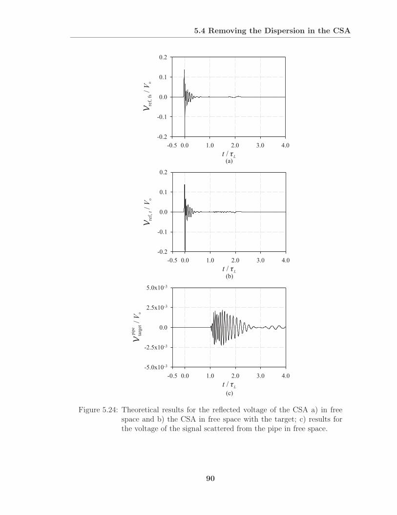
5.4 Removing the Dispersion in the CSA
-0.5 0.0 1.0 2.0 3.0 4.0
-0.2
-0.1
0.0
0.1
0.2
t / L
Vre
f,fs
/V
o
(a)
-0.5 0.0 1.0 2.0 3.0 4.0
-0.2
-0.1
0.0
0.1
0.2
t / L
Vre
f,t/
Vo
(b)
-0.5 0.0 1.0 2.0 3.0 4.0
-5.0x10⁻³
-2.5x10⁻³
0.0
2.5x10⁻³
5.0x10⁻³
Vta
rget
/V
o
t / L
(c)
pip
e
Figure 5.24: Theoretical results for the reflected voltage of the CSA a) in freespace and b) the CSA in free space with the target; c) results forthe voltage of the signal scattered from the pipe in free space.
90

5.4 Removing the Dispersion in the CSA
AnisotropicMaterial
…
…
…
LHCP
LHCP
Left-handed CSA
Grid
……
…
…LHCP
LHCP
Left-handed CSA
RHCP
(a)
(b)
12
12
Figure 5.25: Examples for scatterers of co polarization using a) an anisotropicmedium and b) a grid of closely spaced wires.
Section 5.3.1 that a thin metallic rod scatters predominantly linear polarization that
can be decomposed equally into left-handed and right-handed circular components.
The scattering characteristics of the grid are quantified in Fig. 5.26. The circularly
polarized components of the scattered electric field, Eref,grid, i.e., the difference of the
electric field with and without the grid present, are shown as a function of frequency.
Again, the scattered electric field is normalized by the LHCP component of the in-
cident electric field for the CSA in free space, ELHCPinc , and observed on axis 0.5 cm
91

5.4 Removing the Dispersion in the CSA
0.5 1.0 2.0 3.0 4.0
0.00
0.25
0.50
0.75
1.00
f [GHz]
|EE
ref,
gri
din
c/
|L
HC
P
LHCPRHCP
Figure 5.26: Theoretical results for the circularly polarized components of theelectric field scattered from the grid, normalized by the incident,LHCP component of the electric field.
above the apex. It can be seen that the grid scatters linear polarization since the two
circularly polarized components are almost equal. The relative amplitudes of these
components confirm the simple argument in Fig. 5.25b: The incident LHCP signal
is reflected equally into LHCP and RHCP signals, with the magnitude of each scat-
tered signal being half that of the incident signal, i.e., ELHCPref,grid = ERHCP
ref,grid = 0.5ELHCPinc .
Consequently, the transfer function of the target can be written as F LHCPtarget,grid = −0.5,
neglecting the propagation to and from the grid. The transfer function for the CSA
can thus be determined from (5.11) to be
FCSA(ω) =Vtarget
Vinc F LHCPtarget,grid
= −2 V gridref,t − Vref,fs
Vinc. (5.12)
To determine FCSA, it is only necessary to measure the reflected voltages of the CSA
with and without the grid present. Once FCSA is determined, it can be used to remove
the dispersion from the voltage of a signal scattered from any other target, e.g., that
shown in Fig. 5.24c. The spectrum of the dispersion-less voltage of the signal scattered
from any target is
V disp.lesstarget (ω) =
VtargetFCSA
= −12
Vref,t − Vref,fs
V gridref,t − Vref,fs
Vinc. (5.13)
The results for this voltage when transformed into the time domain are unsatisfactory,
92
5.4 Removing the Dispersion in the CSA
because spurious reflections are superimposed on the signal scattered by the target.
To eliminate these spurious reflections, it is necessary for the spectrum of this voltage
to be smoothly tapered to zero at the limits of the operational frequency range, which
is illustrated in Fig. 5.27a. The dashed line is for the raw results for this voltage,
while the solid line is for the smoothly tapered voltage.
The result for the time-domain voltage scattered from the pipe in free space is
then shown in Figs. 5.27b and c as a function of normalized time t/τL. Notice that
the reflected signal is, as expected, centered around t/τL ≈ 1. By placing the grid
at the apex of the CSA, the spectral components of the modified signals, (5.13), are
delayed such that each frequency of this signal is received at t/τL = 0 when reflected
from the apex. Since the pipe is 1m below the apex of the CSA, the scattered signal
must enter the antenna response at t/τL ≈ 2τs/τL ≈ 1. Clearly, the reflected signal
is not a chirp signal any more, compare with Fig. 5.24c. Instead, it resembles the
differentiated version of the incident pulse, which is due to the transfer function of this
particular target, i.e., the infinite pipe of square cross section scatters approximately
the derivative of the incident signal.
The remainder of this section is concerned with a practical approach for the
pulsed CSA in a monostatic GPR to improve and clarify the time-domain signature
of targets buried in the ground, e.g., for its use in detecting long, perfectly conducting
pipes buried at large depths in the ground. This GPR uses a CSA with the geometry
θ = 7.5, α = 75, δ = 90, and D/d = 8 (d = 6 cm). Notice that this is a
scaled version of the CSA used in the previous example, which was for free space.
All of the dimensions are three times larger and the operational bandwidth is lower
in frequency by a factor of three. The ground is dry soil, which has the following
electrical properties within this bandwidth: εrg ≈ 4 and σg ≈ 0.007 S/m. The same
pipe as in the previous example is used, buried at the depth of 1m in the ground. A
schematic drawing of this radar is shown in Fig. 5.28. Notice that the apex of the
CSA is again located at the air/ground interface, by setting h = 22.8 cm.
The procedure to remove the dispersion from the voltage and thus to determine
93

5.4 Removing the Dispersion in the CSA
0.50 0.75 1.00 1.25 1.50
-15x10-3
-10x10-3
-5x10⁻³
0.0
5x10⁻³
10x10-3
15x10-3
t / L
(c)
Vta
rget
/V
o
dis
p.le
ss
0.5 1.0 1.5 2.0 2.5 3.0 3.5
0.00
0.01
0.02
0.03
0.04
0.05
-0.5 0.0 1.0 2.0 3.0 4.0
-15x10-3
-10x10-3
-5x10⁻³
0.0
5x10⁻³
10x10-3
15x10-3
t / L
(b)
Vta
rget
/V
o
dis
p.le
ss
|VV
targ
et/
inc|
dis
p.le
ss
f [GHz](a)
Tapered VoltageRaw Voltage
Figure 5.27: Theoretical results for the received voltage of the signal scatteredfrom the pipe in free space with the dispersion removed: a) signalin the frequency domain, b) signal in the time domain for −0.5 ≤t/τL ≤ 4, and c) signal in the time domain for 0.5 ≤ t/τL ≤ 1.5.
94

5.4 Removing the Dispersion in the CSA
Earth
s
w
w
h
…
…
Figure 5.28: Schematic model for a monostatic radar to detect the infinitely longpipe buried in the ground.
the signature of this buried target is similar to the one outlined above. First, the
following reflected voltages must be determined separately: the reflected voltage of
the CSA in free space over the ground, first with the target in the ground, Vref,t,and then without the target in the ground, Vref,g. In Fig. 5.29a, the theoretical
result for the reflected voltage of the CSA over the ground with the pipe buried
in the ground is shown as a function of normalized time t/τL. Again, the drive-
point reflection clearly dominates the reflected voltage, since the reflections from the
air/ground interface and the target are small compared with this initial reflection
at t/τL ≈ 0. In Fig. 5.29b, the voltage for the signal scattered from the target,
Vtarget(t) = Vref,t−Vref,g, is shown. Due to the presence of the ground, the time for anelectromagnetic wave to propagate the distance s from the apex to the target is now
τs =√εrgs/c, or, in this example, in normalized form τs/τL =
√εrgs/Ls = 0.3. The
95

5.4 Removing the Dispersion in the CSA
-0.5 0.0 1.0 2.0 3.0 4.0
-1x10⁻³
0.5x10⁻³
0
0.5x10⁻³
1x10⁻³
-0.5 0.0 1.0 2.0 3.0 4.0
-0.2
-0.1
0.0
0.1
0.2
t / L
Vre
f,t/
Vo
(a)
Vta
rget
/V
o
t / L
(b)
rod
Figure 5.29: Theoretical results for a) the reflected voltage of the CSA above thedry ground with the pipe present and b) the voltage of the signalscattered from the pipe.
scattered signal in Fig. 5.29b is a chirp signal with the highest frequencies arriving
first at t/τL ≈ [2(hc − hs) + 2√εrgs]/Ls = 0.7 and the lowest frequencies arriving
last at t/τL ≈ [2Ls + 2hc + 2√εrgs]/Ls = 3.2. Similar to the previous example, the
dispersion can be removed using the transfer function of the CSA, FCSA, obtained
by subtracting the reflected voltages of the CSA in free space with and without the
grid in free space, see (5.12). The spectrum of the dispersion-less voltage can thus be
written as
V disp.lesstarget (ω) =
VtargetFCSA
= −12
Vref,t − Vref,g
V gridref,t − Vref,fs
Vinc. (5.14)
This voltage, when tapered at the limits of the operational frequency range and
then Fourier transformed, is graphed in Fig. 5.30 and shows a pulse centered at
96
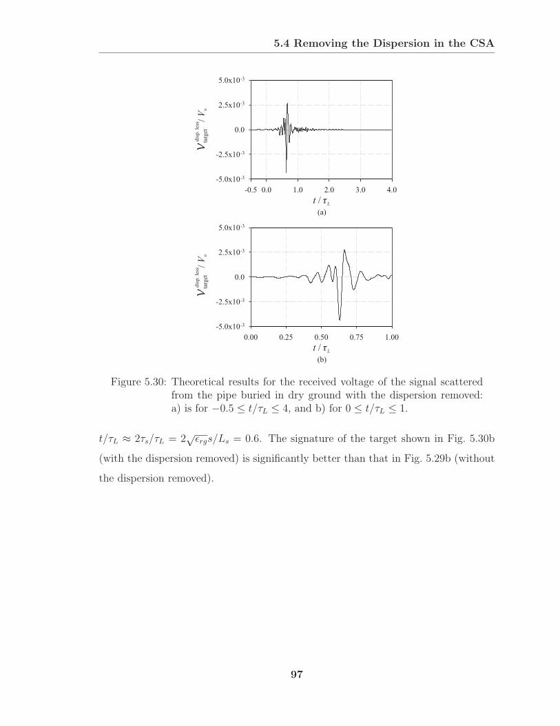
5.4 Removing the Dispersion in the CSA
0.00 0.25 0.50 0.75 1.00
-5.0x10⁻³
-2.5x10⁻³
0.0
2.5x10⁻³
5.0x10⁻³
-0.5 0.0 1.0 2.0 3.0 4.0
-5.0x10⁻³
-2.5x10⁻³
0.0
2.5x10⁻³
5.0x10⁻³
t / L
(a)
Vta
rget
/V
o
dis
p.le
ss
t / L
(b)
Vta
rget
/V
o
dis
p.le
ss
Figure 5.30: Theoretical results for the received voltage of the signal scatteredfrom the pipe buried in dry ground with the dispersion removed:a) is for −0.5 ≤ t/τL ≤ 4, and b) for 0 ≤ t/τL ≤ 1.
t/τL ≈ 2τs/τL = 2√εrgs/Ls = 0.6. The signature of the target shown in Fig. 5.30b
(with the dispersion removed) is significantly better than that in Fig. 5.29b (without
the dispersion removed).
97
CHAPTER 6
FDTD Analysis
This chapter is concerned with the finite-difference time-domain (FDTD) method in
three-dimensions for its use in the analysis and design of antennas. Since then, the
FDTD method is a time-domain method in which transient fields are computed as
a function of time, and which allows the accurate characterization of complex in-
homogeneous structures for which analytical methods are ill-suited. The genesis of
this numerical method in electromagnetics was in the work of Yee in 1966 [28]. In
his seminal paper, he proposed a three-dimensional central difference approximation
for Maxwell’s curl equations, both in space and time. The FDTD method has been
applied to many areas in electromagnetics and documented extensively in the litera-
ture [29]-[31]. With increasing computational power,1 the FDTD method has evolved
as one of the most popular and powerful numerical methods over the last decade,
particularly for its use in analyzing and designing antennas [33]-[35]. This numeri-
cal method, inherently a time-domain technique, is especially beneficial in analyzing
broadband antennas such as the conical spiral antenna (CSA), because antenna char-
acteristics can be obtained over a broad range of operating frequencies with just a
single simulation; compare this with a series of simulations that would be necessary
with a frequency-domain method, e.g. Finite Elements or Method of Moments.
Section 6.1 is mainly concerned with the derivation of a single set of update
1Following Moore’s Law [32], the computational power (precisely, the number of transistors per
integrated circuit) approximately doubles every 18 months.
98
6.1 FDTD Update Equations
equations that applies to all media used in the problem, i.e., free space, conductive
ground, and the conductive, uniaxial, anisotropic medium used to implement the
perfectly matched layer (PML) absorbing boundary condition. Section 6.2 verifies
that this absorbing boundary condition absorbs outgoing electromagnetic energy with
negligible reflection. The two-step discretization scheme of CSAs is outlined in Section
6.3, while the discretization of the feed region and the feeding technique with a virtual
transmission line are described in Section 6.4. To obtain the electric fields in the far
zone of the antenna, a near-field to far-field transformation must be employed; the
governing convolution is discussed rather briefly in Section 6.5 for the CSA isolated
in free space. Section 6.6 outlines the savings in execution time by parallelizing the
computer code and running the simulations on multiple-processor architectures.
6.1 FDTD Update Equations
The objective of this section is to derive a single set of FDTD update equations
that is general enough to be applied to all media present in the problem studied. In
Section 6.1.1, the differential forms of Faraday’s Law and the Ampere-Maxwell Law
are presented for conductive, uniaxial, anisotropic media, used to implement the per-
fectly matched layer (PML) absorbing boundary condition. The electric properties
of this medium are sufficient to describe the media of interest in this work. This
layer truncates the open region surrounding the antenna and effectively extends this
region to infinity by absorbing all impinging waves. In Section 6.1.2, Maxwell’s curl
equations in continuous space are discretized with the approach suggested by Yee in
1966: central differences in time and space. Furthermore, an efficient implementa-
tion of these update equations in the computer program is introduced. Section 6.1.3
is concerned with the correct averaging of the electrical properties (µr, εr, σ) at me-
dia interfaces and the spatial distribution of the electrical parameters of PML. The
CSA terminations (lumped resistor and resistive sheet) require modification of the
electromagnetic fields in the vicinity of the resistive elements, which is described in
99
6.1 FDTD Update Equations
Section 6.1.4. Section 6.1.5 outlines the implementation of dipole antennas with finite
thickness in the FDTD method.
6.1.1 Update Equations in Continuous Space
In this research, the CSA is investigated when isolated in free space or in free
space placed directly over the ground. This problem, as almost all antenna prob-
lems/applications, is an open-region problem in which the media surrounding the
antenna extend to infinity. Obviously, the infinite space cannot be modeled numer-
ically, so the region surrounding the antenna must be truncated by an absorbing
boundary condition, which should ideally absorb any outgoing electromagnetic radi-
ation and thus simulate the extension of the studied domain to infinity. Hence, the
reception/transmission characteristics or the near field of the antenna can be deter-
mined explicitly, while the field in the far zone can only be determined using near-field
to far-field transformations, discussed in Section 6.5. Over the last decade, absorbing
boundary conditions have been developed that absorb electromagnetic waves with
negligible reflection independent of the frequency, polarization, and angle incident
upon the interface. The genesis of these PML absorbing boundary conditions was
in the work of Berenger [36]. He proposed to replace the medium surrounding the
studied geometries with a highly effective absorbing material of finite thickness, dPML,
shown schematically in Fig. 6.1. The computational domain of this open-region prob-
lem is truncated by the PML and is thus bounded in length (X), width (Y ), and
height (Z). In continuous space, the electrical properties of the PML can be perfectly
matched to those of the ambient medium to result in a vanishing reflection coeffi-
cient. Upon discretization, this absorbing material must be adjusted appropriately to
absorb the outgoing electromagnetic energy with negligible reflection. The uniaxial
material method [37, 38] is more demonstrative and more efficient than Berenger’s
original formulation that involved the splitting of fields, and thus causes computa-
tionally expensive modifications of Maxwell’s equations. The complex coordinate
100

6.1 FDTD Update Equations
x
y
z
X
dPML
Z
YPML
Ground
Air
Figure 6.1: Schematic drawing for the open-region problem truncated by thePML absorbing boundary condition (CSA is omitted for simplicity).
stretching method is another straightforward approach to formulate the PML, which
can easily be applied to spherical and cylindrical coordinate systems [39]. Although
the PML absorbing boundary condition is computationally more expensive than for-
merly used absorbing boundary conditions, the reflections from the truncated grid are
reduced significantly and almost independent of frequency, polarization, and angle of
incidence.
The PML formulation used in this research is based on Gedney’s uniaxial PML
[40]. The electrical properties of the conductive, uniaxial, anisotropic material are
described by tensors with zero off-diagonal entries. To achieve a perfect match be-
tween the open region surrounding the antenna and the PML, the tensors for the
permittivity, ε, and the permittivity, µ, have to satisfy
ε
εεr=
µ
µµr
=
syszsx
0 0
0sxszsy
0
0 0sxsysz
. (6.1)
101

6.1 FDTD Update Equations
The tensor elements can be written as
si = κi +σi
jωεwith i = x, y, z (6.2)
and correspond to loss terms in the longitudinal direction i. The purely real term
κi ≥ 1 is intended to suppress evanescent modes,2 while the anisotropic conductivity
σi is intended to suppress the propagating modes within the thin layer. To match
the ambient medium to the PML, it must extend through the PML with the same
µr, εr, and σ, i.e., the PML is defined electrically by the set of anisotropic conductiv-
ities (σx, σy, σz) and the set of isotropic properties (µr, εr, σ) of the ambient medium.3
When using the phasor notation,4 the relative permittivity εr and the conductivity σ
are often combined in the complex permittivity
εr = εr(1− jp) = εr
(1− j
σ
ωεεr
), (6.3)
where p is the loss tangent p = σ/(ωεεr).
The governing FDTD update equations are based on Maxwell’s curl equations;
therefore, the transient electromagnetic fields within conductive, uniaxial, anisotropic
media will eventually be computed from Faraday’s Law
∇× &E = −jωµ &H (6.4)
and the Ampere-Maxwell Law
∇× &H = jωε &E. (6.5)
2In this research, κi = 1 is chosen.3Notice the difference between the conductivities σ and σi: While σ describes the isotropic
conduction loss, e.g., in the ground, σi describes the anisotropic conduction loss along its longitudinal
direction.4The vector phasor F (ω) is defined with
F(t) = Re
F (ω)ejωt
,
where F(t) is the time-harmonic function. Notice that throughout this work, the time-domainvariables are shown with a calligraphic font, while phasors are shown with a roman font.
102

6.1 FDTD Update Equations
Writing out the tensors and arranging terms to form dimensionless quantities, (6.4)
can be rewritten as
(Ls∇)× &E ′ = −jωτLµr
syszsx
0 0
0sxszsy
0
0 0sxsysz
&H ′ (6.6)
and (6.5) as
(Ls∇)× &H ′ = (ησLs + jωτLεr)
syszsx
0 0
0sxszsy
0
0 0sxsysz
&E ′. (6.7)
In the above equations, each of the terms is a dimensionless quantity. The parameters
used for normalization are the length of the spiral arms, Ls, the characteristic time
of the antenna, τL = Ls/c, and the free-space wave impedance, η. Notice that the
primed fields, &E ′ and &H ′, are normalized as well, i.e., the normalized electric field is
&E ′ =&E
(V/Ls)(6.8)
and the normalized magnetic field is
&H ′ =η &H
(V/Ls), (6.9)
where V is the peak of the incident voltage used to excite the antenna, see (2.9).
In the remainder of this chapter, just the x components of Maxwell’s curl equa-
tions will be investigated for simplicity and then used to derive the FDTD update
equations for the electric field, E ′x, and the magnetic field, H′
x. The y and z com-
ponents of these fields can be derived similarly and are omitted here. Consequently,
Faraday’s Law (eventually used to determine H′x) is
∂E ′z
∂(y/Ls)− ∂E ′
y
∂(z/Ls)= −jωτLµr
syszsx
H ′x, (6.10)
103

6.1 FDTD Update Equations
and the Ampere-Maxwell Law (eventually used to determine E ′x) is
∂H ′z
∂(y/Ls)− ∂H ′
y
∂(z/Ls)= (ησLs + jωτLεr)
syszsx
E ′x. (6.11)
These equations contain several mixed jω terms (both in the numerator and de-
nominator) that yield convolutions when transformed to the time domain. Numer-
ically, such convolutions are computationally expensive and can be avoided by de-
coupling (6.10) and (6.11) [37]. Consequently, multiple-step update equations will
result. For the central finite-difference scheme of second order, each decoupled up-
date equation must have at most one frequency-dependent term of the form a+ jωb,
e.g., ησyLs + jωτLsy = jωτL, in the numerator. Introducing the “dummy” field
Bx = sz/sx H′x or equivalently jωτLsx Bx = jωτLsz H
′x, Faraday’s Law (6.10) can
be decoupled and the following two-step update equation for the magnetic field H ′x
results: step 1 is
−µr(ησyLs + jωτL)Bx =∂E ′
z
∂(y/Ls)− ∂E ′
y
∂(z/Ls)(6.12)
and step 2
(ησzLs + jωτL)H′x = (ησxLs + jωτL)Bx. (6.13)
Obviously, this dummy field Bx causes an increase of memory requirements in the
computer simulation but is computationally less expensive than convolutions. Note
that this field does not correspond to the magnetic flux, &B = µ &H; this is just the no-
tation commonly used in the literature. Introducing the dummy fields Dx = sz/sx E′x
and Fx = sy Dx, the Ampere-Maxwell Law (6.11) can be decoupled and the following
three-step5 update equation for the electric field E ′x results: step 1 is
(ησLs + jωτLεr)Fx =∂H ′
z
∂(y/Ls)− ∂H ′
y
∂(z/Ls), (6.14)
step 2
(ησyLs + jωτL)Dx = jωτLFx, (6.15)
5Here, the frequency-dependent term introduced by the isotropic conductivity of the medium, σ,
causes an additional step compared to the two steps required to solve for the magnetic field.
104

6.1 FDTD Update Equations
and step 3
(ησzLs + jωτL)E′x = (ησxLs + jωτL)Dx. (6.16)
Since the frequency-dependent terms in Maxwell’s curl equations are decoupled,
(6.12)-(6.16) can be conveniently transformed to the time domain by replacing the
jωτL terms with time derivatives∂
∂(t/τL). Therefore, the time-domain form of Fara-
day’s Law in continuous space can be written in step 1
−ησyLsµr Bx − µr∂Bx
∂(t/τL)=
∂E ′z
∂(y/Ls)− ∂E ′
y
∂(z/Ls)(6.17)
and in step 2
ησzLs H′x +
∂H′x
∂(t/τL)= ησxLs Bx +
∂Bx
∂(t/τL)(6.18)
Similarly, the time-domain form of the Ampere-Maxwell Law in continuous space can
be written in step 1
ησLs Fx + εr∂Fx
∂(t/τL)=
∂H′z
∂(y/Ls)− ∂H′
y
∂(z/Ls), (6.19)
in step 2
ησyLs Dx +∂Dx
∂(t/τL)=
∂Fx
∂(t/τL), (6.20)
and in step 3
ησzLs E ′x +
∂E ′x
∂(t/τL)= ησxLs Dx +
∂Dx
∂(t/τL). (6.21)
In the next section, these equations will be discretized following Yee’s approach to
obtain typical FDTD update equations.
6.1.2 Update Equations in Discretized Space
The spatial discretization of the update equations for the electric and magnetic fields,
derived in the previous section, is based on the Yee cell [28], shown in Fig. 6.2. The
dimensions of the cube are denoted by ∆x,∆y, and ∆z for its length, width, and
height. The Yee cell is the basic building block of the computational domain and
used to discretize and model arbitrary structures of complex composition. Notice
105

6.1 FDTD Update Equations
that the magnetic fields are normal to the sides of the cell and determined at the
center of the sides, while the electric fields are tangential to the edges of the cell
and determined at the center of the edges. The discretization in time is such that
the magnetic fields are evaluated at half time steps, i.e., t = (n + 0.5)∆t, while the
electric fields are evaluated at full time steps, i.e., t = (n + 1)∆t. Throughout this
work, a short-hand notation for the field components is used, e.g., the normalized
x component of the electric field is referred to as E ′x|n+1i,j,k = E ′n+1
x (i, j, k) = E ′x(x =
(i−0.5)∆x, y = (j−1)∆y, z = (k−1)∆z, t = (n+1)∆t). A list of staggered positions
in time and space for all electric and magnetic fields within the Yee cell (i, j, k) is
presented in Table 6.1. It is important to note that the spatial indices (i, j, k) refer to
the cell in which the field components are located rather than to the actual positions
of the field components in the grid. Notice also that the fields that are referred to
cell (i, j, k) are shown with black symbols in the Yee cell, Fig. 6.2, while the gray field
components belong to neighboring cells.
In the following, Maxwell’s Equations (6.17)-(6.21) will be discretized to obtain
the typical FDTD update equations, so that the transient fields can be computed using
the well-known “leapfrog” scheme of the FDTD, i.e., the update of the magnetic field
x
y
z
Hz
Ex
Ey
Ez
Hx
Hy
y
x
z
Yee Cell ( , , ):i j k
[ ]( -1) , ( -1) , ( -1) )i x j y k z
Figure 6.2: Yee cell in three dimensions.
106
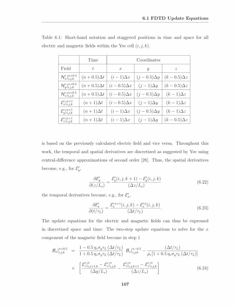
6.1 FDTD Update Equations
Table 6.1: Short-hand notation and staggered positions in time and space for all
electric and magnetic fields within the Yee cell (i, j, k).
Time Coordinates
Field t x y z
H′x|n+0.5i,j,k (n+ 0.5)∆t (i− 1)∆x (j − 0.5)∆y (k − 0.5)∆z
H′y|n+0.5i,j,k (n+ 0.5)∆t (i− 0.5)∆x (j − 1)∆y (k − 0.5)∆z
H′z|n+0.5i,j,k (n+ 0.5)∆t (i− 0.5)∆x (j − 0.5)∆y (k − 1)∆z
E ′x|n+1i,j,k (n+ 1)∆t (i− 0.5)∆x (j − 1)∆y (k − 1)∆z
E ′y|n+1i,j,k (n+ 1)∆t (i− 1)∆x (j − 0.5)∆y (k − 1)∆z
E ′z|n+1i,j,k (n+ 1)∆t (i− 1)∆x (j − 1)∆y (k − 0.5)∆z
is based on the previously calculated electric field and vice versa. Throughout this
work, the temporal and spatial derivatives are discretized as suggested by Yee using
central-difference approximations of second order [28]. Thus, the spatial derivatives
become, e.g., for E ′y,
∂E ′y
∂(z/Ls)=
E ′y(i, j, k + 1)− E ′
y(i, j, k)
(∆z/Ls)(6.22)
the temporal derivatives become, e.g., for E ′x,
∂E ′x
∂(t/τL)=
E ′n+1x (i, j, k)− E ′n
x (i, j, k)
(∆t/τL). (6.23)
The update equations for the electric and magnetic fields can thus be expressed
in discretized space and time: The two-step update equations to solve for the x
component of the magnetic field become in step 1
Bx|n+0.5i,j,k =1− 0.5 ησyτL (∆t/τL)
1 + 0.5 ησyτL (∆t/τL)Bx|n−0.5i,j,k − (∆t/τL)
µr[1 + 0.5 ησyτL (∆t/τL)]
×[ E ′
z|ni,j+1,k − E ′z|ni,j,k
(∆y/Ls)− E ′
z|ni,j,k+1 − E ′z|ni,j,k
(∆z/Ls)
](6.24)
107
6.1 FDTD Update Equations
and in step 2
H′x|n+0.5i,j,k =
1− 0.5 ησzτL (∆t/τL)
1 + 0.5 ησzτL (∆t/τL)H′
x|n−0.5i,j,k +1
1 + 0.5 ησzτL (∆t/τL)
×[1 + 0.5 ησxτL (∆t/τL)] Bx|n+0.5i,j,k
+ [−1 + 0.5 ησxτL (∆t/τL)] Bx|n−0.5i,j,k
. (6.25)
Similarly, the three-step update equations to solve for the x component of the electric
field become in step 1
Fx|n+1i,j,k =εr − 0.5 ηστL (∆t/τL)
εr + 0.5 ηστL (∆t/τL)Fx|ni,j,k +
(∆t/τL)
εr + 0.5 ηστL (∆t/τL)
×H′
z|n+0.5i,j+1,k − H′z|n+0.5i,j,k
(∆y/Ls)− H′
z|n+0.5i,j,k+1 − H′z|n+0.5i,j,k
(∆z/Ls)
, (6.26)
in step 2
Dx|n+1i,j,k =1− 0.5 ησyτL (∆t/τL)
1 + 0.5 ησyτL (∆t/τL)Dx|ni,j,k
+1
1 + 0.5 ησyτL (∆t/τL)
(Fx|n+1i,j,k − Fx|ni,j,k
), (6.27)
and in step 3:
E ′x|n+1i,j,k =
1− 0.5 ησzτL (∆t/τL)
1 + 0.5 ησzτL (∆t/τL)E ′x|ni,j,k +
1
1 + 0.5 ησzτL (∆t/τL)
×[1 + 0.5 ησxτL (∆t/τL)] Dx|n+1i,j,k
+ [−1 + 0.5 ησxτL (∆t/τL)] Dx|ni,j,k. (6.28)
In (6.24) and (6.25), the fields Bx and H′x must be interpolated at times t = n∆t since
they do not exist at the full time steps, e.g., Bnx = 0.5(Bn+0.5
x + Bn−0.5x ), similarly in
(6.26)-(6.28) the fields Fx,Dx, and E ′x must be interpolated at times t = (n+0.5)∆t.
Obviously, the above equations are rather complex, so the following technique is used
108

6.1 FDTD Update Equations
in the computer program to simplify their structure and to optimize the updating
procedure. Equations (6.24)-(6.28) are therefore expressed using “update variables”
that contain the terms in front of the field components. For the magnetic field, step
1 becomes
Bx|n+0.5i,j,k = upd Bx1(j)Bx|n−0.5i,j,k
+ upd Bx2(j)
[E ′z|ni,j+1,k − E ′
z|ni,j,k(∆y/Ls)
− E ′z|ni,j,k+1 − E ′
z|ni,j,k(∆z/Ls)
](6.29)
and step 2
H′x|n+0.5i,j,k = upd Hx1(k)H′
x|n−0.5i,j,k + upd Hx2(i, k)Bx|n+0.5i,j,k
+ upd Hx3(i, k)Bx|n−0.5i,j,k . (6.30)
For the electric field, step 1 becomes
Fx|n+1i,j,k = upd Fx1(i, j, k)Fx|ni,j,k
+ upd Fx2(i, j, k)
[H′z|n+0.5i,j+1,k −H′
z|n+0.5i,j,k
(∆y/Ls)− H′
z|n+0.5i,j,k+1 −H′z|n+0.5i,j,k
(∆z/Ls)
],(6.31)
step 2
Dx|n+1i,j,k = upd Dx1(j)Dx|ni,j,k
+ upd Dx2(j)(Fx|n+1i,j,k −Fx|ni,j,k
), (6.32)
and step 3:
E ′x|n+1i,j,k = upd Ex1(k) E ′
x|ni,j,k + upd Ex2(i, k)Dx|n+1i,j,k
+ upd Ex3(i, k)Dx|ni,j,k. (6.33)
Notice that the update variables in the above equations are one, two or three-
dimensional. This is mainly because the terms in the update variables contain a
109

6.1 FDTD Update Equations
combination of PML conductivities σi. While the anisotropic conductivities, σi, can
be constant in continuous space to satisfy the matching condition, (6.1), the σi must
be tapered from zero (at the PML interface) to σi,max (at the outer grid boundary) in
discretized space along their longitudinal direction to effectively absorb the outgoing
waves,6 i.e., σx = σx(i), σy = σy(j), and σz = σz(k). In the above equations, it was
furthermore assumed that the isotropic conductivity is piecewise constant along the
z direction, i.e., σ = σ(k), and that the permittivity can be piecewise constant in any
direction, i.e., εr = εr(i, j, k). The advantage of this implementation of the FDTD
equations is that the update variables can be calculated once in the initialization
stage of the computer program and then used throughout the rest of the program,
i.e., for the update of &E and &H. It is therefore not necessary to perform the costly
operations of calculating these terms every time the fields are updated. The draw-
back of this approach is that especially the 3D variables, e.g., upd Fx1 and upd Fx2,
require a significant amount of memory for the computer simulation to run.7 For the
program to run most time efficient on common computer architectures, it is often
most important to reduce the number of floating-point operations instead of reducing
the memory consumption.
6.1.3 Medium Properties in the FDTD Update Equations
Various isotropic media are used in problems studied, e.g., that in which the CSA in
free space is placed directly over the ground to detect mines buried in the ground.
This open region is divided into the free-space region that can be described with
the electrical properties (µr = 1, εr = 1, and σ = 0), the soil with the electrical
properties (µrg = 1, εrg > 1, and σg > 0), and the mine with the electrical properties
6The anisotropic conductivities must be tapered within the PML because the discontinuity would
otherwise cause significant artificial reflections.7Some versions of the computer code are based on a hybrid approach, in which the 1D and 2D
update variables are implemented as shown, while the fields F are updated explicitly without the
3D update variables.
110
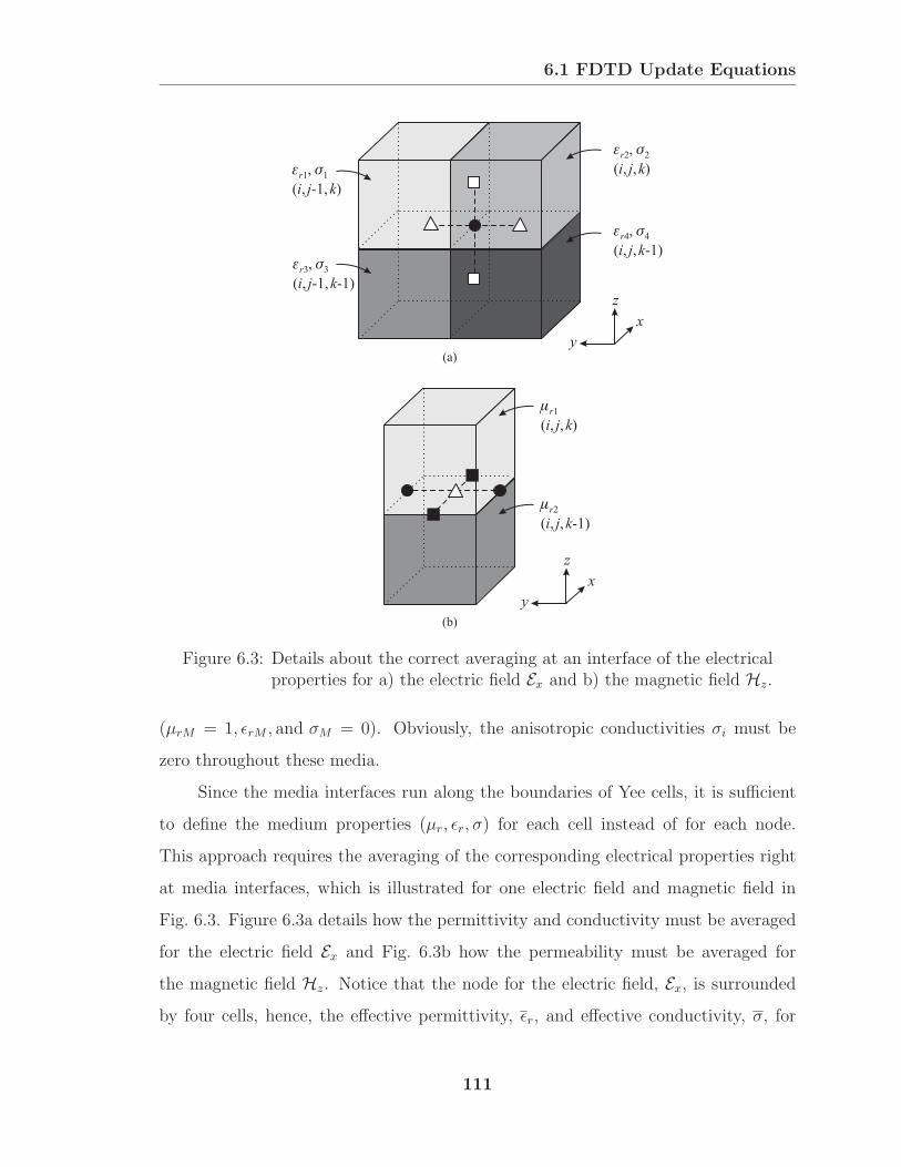
6.1 FDTD Update Equations
r1 1,
( , -1, )i j k
r1
( , , )i j k
r2 2,
( , , )i j k
r3 3,
( , -1, -1)i j k
r2
( , , -1)i j k
r4 4,
( , , -1)i j k
(a)
(b)
x
y
z
x
y
z
Figure 6.3: Details about the correct averaging at an interface of the electricalproperties for a) the electric field Ex and b) the magnetic field Hz.
(µrM = 1, εrM , and σM = 0). Obviously, the anisotropic conductivities σi must be
zero throughout these media.
Since the media interfaces run along the boundaries of Yee cells, it is sufficient
to define the medium properties (µr, εr, σ) for each cell instead of for each node.
This approach requires the averaging of the corresponding electrical properties right
at media interfaces, which is illustrated for one electric field and magnetic field in
Fig. 6.3. Figure 6.3a details how the permittivity and conductivity must be averaged
for the electric field Ex and Fig. 6.3b how the permeability must be averaged for
the magnetic field Hz. Notice that the node for the electric field, Ex, is surrounded
by four cells, hence, the effective permittivity, εr, and effective conductivity, σ, for
111

6.1 FDTD Update Equations
Table 6.2: Averaging of the electrical properties in the FDTD update equa-tions.
Updated Field Averaged Medium Property
H′x|n+0.5i,j,k µr =
µr(i,j,k)+µr(i−1,j,k)2
H′y|n+0.5i,j,k µr =
µr(i,j,k)+µr(i,j−1,k)2
H′z|n+0.5i,j,k µr =
µr(i,j,k)+µr(i,j,k−1)2
E ′x|n+1i,j,k εr =
εr(i,j,k)+εr(i,j−1,k)+εr(i,j,k−1)+εr(i,j−1,k−1)4
E ′y|n+1i,j,k εr =
εr(i,j,k)+εr(i−1,j,k)+εr(i,j,k−1)+εr(i−1,j,k−1)4
E ′z|n+1i,j,k εr =
εr(i,j,k)+εr(i−1,j,k)+εr(i,j−1,k)+εr(i−1,j−1,k)4
this node are the average of the electrical properties εr and σ of the surrounding
cells. Similarly, the node for the magnetic field is surrounded by two cells, hence,
the effective permeability, µ, for this node is the average of the permeabilities of the
surrounding cells. The proper averaging of the electrical properties is outlined in
Table 6.2 for the electric8 and magnetic fields.
The PML, truncating the region surrounding the antenna can be subdivided in
three general regions: corners, edges, and sides. Within these regions, the anisotropic
conductivities σi are nonzero when the PML extends in the longitudinal direction
and zero when it extends in any transverse direction, e.g., σx = σx(i) = 0 for the
PML extending along x, and σx = 0 for the PML extending along y and z. Hence,
in the corners all conductivities σi are nonzero, in edges only two conductivities σi
are nonzero, e.g., σx = σx(i) = 0 and σy = σy(j) = 0 for the edge region with PMLinterfaces normal to x and y direction, and in the sides only one σi is nonzero, e.g.,
σx = 0 for the side region with a PML interface normal to the x direction.
In Fig. 6.4a, the variation of the conductivity σx along the longitudinal direc-
tion x is illustrated. The conductivity is zero within the open region surrounding
8The averaging technique for the conductivity σ is the same as for the permittivity εr (replace
εr with σ).
112

6.1 FDTD Update Equations
x,max
x
dPML X-dPML X
( -1)i x ( -0.5)i x
Cell ( , , )i j k
x
(a)
(b)
Air ( = 1)r
Ground ( , ) rg g
PML
z
x
m sx,air
m sx,ground
PEC
Figure 6.4: a) Spatial variation of the conductivity σx a) along its longitudi-nal direction x and b) along its transverse direction z with theair/ground interface present.
the antenna and tapered from zero at the interface between the open region and the
PML to the maximum value σx,max at the outermost boundaries of the computational
domain.9 Commonly, a polynomial taper is chosen to mathematically express the con-
ductivities σi along its longitudinal direction [40]. The expression for the normalized
9The optimum value for σi,max must be a trade off between two different types of reflection. When
the value for σi,max is chosen too small, waves are barely attenuated within the PML and reflect
from the PEC interface that is behind the PML. When the value for σi,max is too big, significant
reflections occur from within the PML due to large medium discontinuities between cells.
113

6.1 FDTD Update Equations
conductivity ησxLs, as it appears in the update equations, can thus be written
ησxLs =
ησx,maxLs
(dPML−xdPML
)mfor x ≤ dPML
0 for dPML < x < X − dPML
ησx,maxLs
[x−(X−dPML)
dPML
]mfor x ≥ X − dPML
(6.34)
In this research, the exponent of the polynomial taper is chosen to be m = 2.1
[41]. The following rule of thumb for evaluating the maximum value of this taper is
proposed given the thickness of the PML is 10 cells. The condition
ησx,maxLs =τL∆t
(6.35)
should be satisfied to obtain good results for the reflection coefficient from the in-
terface. Notice that this expression can be remembered/derived easily from the
discretized form of the update equations, (6.29)-(6.33). Terms of the form 1 +
0.5ησiLs(∆t/τL) will be become 1 + 0.5 at the outermost boundaries of the com-
putational domain.
For the best PML performance, the anisotropic conductivities must be deter-
mined with respect to the actual position of the node instead of the position of the
cell the field is located in. In the presented case, shown in the inset of Fig. 6.4a,
the update equations for the fields E ′y|i,j,k, E ′
z|i,j,k, and H′x|i,j,k require the calculation
of the conductivity σx at positions x = (i − 1)∆x, while the update equations for
the fields E ′z|i,j,k,H′
y|i,j,k, and H′z|i,j,k require the calculation of the conductivity at
positions x = (i− 0.5)∆x.
When the open region surrounding the antenna is a homogeneous dielectric (εr),
the tensor elements si are often expressed as si = κi+σi/(jωεεr) and thus dependent
on the relative permittivity of the ambient medium. However, when the open region
has media interfaces with piecewise constant εr, e.g., the air/ground interface, the
above expression for si causes an accumulation of charges at these discontinuities and
thus leads to instabilities [40]. To satisfy Gauss’ Law, the si terms can only vary
along its longitudinal direction. Therefore, the imaginary part of si, Imsi must be
114

6.1 FDTD Update Equations
…
…
…
…
RL
Ex ( )i , j ,kL L L
n+1
x
yz
Figure 6.5: Implementing the lumped resistor in the FDTD method.
continuous at interfaces along its transverse directions, as illustrated in Fig. 6.4b for
Imsx along its transverse direction z near the air/ground interface. By expressing
the terms si in (6.2) with εr = 1, the PML is optimized for the free space region.
Since the antenna is located in air, this region has the strongest fields and requires the
best performance. The ground is most often lossy, so that the natural attenuation in
the soil could make up for the increase in the reflection from the PML in the ground.
6.1.4 FDTD Update Equations for the Resistive Elements
This section is concerned with the FDTD update equations for the lumped resistor
elements and the resistive sheet. More detailed discussions on the lumped resistors
can be found in [30] and on the resistive sheet in [42, 43].
To model the lumped resistor, RL, connected at two terminals that extend in
the x direction, consider the schematic drawing in Fig. 6.5. In discretized space, the
implementation of this resistor involves the modification of the tangential electric
fields, Ex, between the terminals. In the presented case, the modification of a single
electric field En+1x (iL, jL, kL) is discussed; however, this analysis can easily be applied
to a multiple-cell gap. When the resistance of the node within this gap is RL, the
115

6.1 FDTD Update Equations
current (measured positive in +x direction) through this node can be expressed as
In+0.5L (iL, jL, kL) =
∆x[En+1x (iL, jL, kL) + En
x (iL, jL, kL)]
2RL
, (6.36)
which is Ohm’s Law. This conduction current must be considered in the derivation
of the update equations for the electric field at this node, i.e., the Ampere-Maxwell
Law must then be
∇× &H = εεr∂ &E∂t+ &JL = εεr
∂ &E∂t+
JL,x
0
0
. (6.37)
Upon discretization of this equation, the new update equation for the electric field
within the gap is
Ex|n+1iL,jL,kL=
1− ∆t∆x2RLεεr∆z∆y
1 + ∆t∆x2RLεεr∆z∆y
Ex|niL,jL,kL+
∆tεεr
1 + ∆t∆x2RLεεr∆z∆y
×(Hz|n+0.5iL,jL+1,kL
−Hz|n+0.5iL,jL,kL
∆y− Hz|n+0.5iL,jL,kL+1
−Hz|n+0.5iL,jL,kL
∆z
).(6.38)
Notice that this update equation is written in its original and, hence, un-normalized
form.
The resistive sheet, commonly characterized by the resistance per square Rs =
1/(σsts) (conductivity σs and thickness ts), covers the cross-sectional area of the big
end of the CSA and thus spreads over a significant number of cells in the computa-
tional grid. However, the thickness of the sheet is just a fraction of the height of the
Yee cell, as shown in Fig. 6.6a; hence, a subcell model must be introduced to include
this thin resistive sheet in the FDTD method. This subcell approach is illustrated in
Fig. 6.6b, which is a cross-sectional view of the modified Yee cell in the xz plane. The
top row of cells contains the resistive sheet, shown in gray, and within these cells a
subcell is introduced. These special cells contain two electric field components Ez: the
electric field in the center of the subcell (resistive sheet), Ez,s, and the regular electric
field in the center of the Yee cell, Ez,r. Reference [42] outlines, how this subcell model
116

6.1 FDTD Update Equations
x
y
z
Hz
Ex
Ey
Ez
Hx
Hy
ts
(a)
(b)
x
z
Ex
Ex
Ex
Ex
Ex
Ex
Ex
Ex
Ex
Ez,r Ez,r
Ez EzEz Ez
Ez,s Ez,sEz,s Ez,s
Ez,r Ez,rHy
Hy
Hy
Hy
Hy
Hy
Subcell
Figure 6.6: Implementing the resistive sheet in the FDTDmethod: a) the three-dimensional Yee cell containing the resistive sheet and b) slice ofthe FDTD grid in the vicinity of the sheet.
modifies the electric and magnetic fields within those special cells, i.e., incorporat-
ing the additional electrical properties and the additional electric field in the FDTD
update equations.
6.1.5 FDTD Update Equations for a Dipole
This section outlines the modeling of linear dipole antennas in the FDTD method.
The schematic model for the dipole of length L and conductor radius a is shown
in Fig. 6.7a. The case investigated in this section is that in which the radius of the
conductor, a, is smaller than the dimensions of the cell size, in particular a < ∆y/2 ≈
117
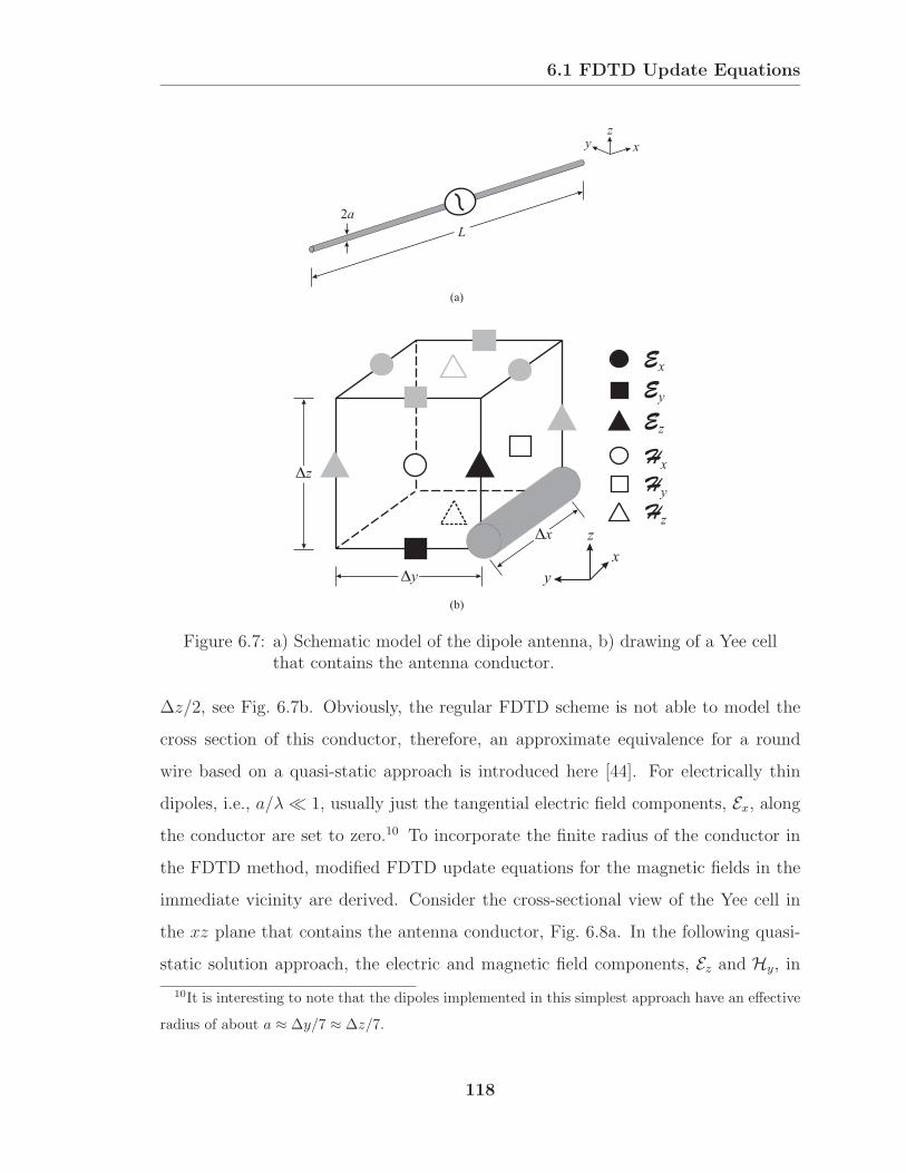
6.1 FDTD Update Equations
xyz
(a)
(b)
L
2a
x
y
z
Hz
Ex
Ey
Ez
Hx
Hy
y
x
z
Figure 6.7: a) Schematic model of the dipole antenna, b) drawing of a Yee cellthat contains the antenna conductor.
∆z/2, see Fig. 6.7b. Obviously, the regular FDTD scheme is not able to model the
cross section of this conductor, therefore, an approximate equivalence for a round
wire based on a quasi-static approach is introduced here [44]. For electrically thin
dipoles, i.e., a/λ 1, usually just the tangential electric field components, Ex, along
the conductor are set to zero.10 To incorporate the finite radius of the conductor in
the FDTD method, modified FDTD update equations for the magnetic fields in the
immediate vicinity are derived. Consider the cross-sectional view of the Yee cell in
the xz plane that contains the antenna conductor, Fig. 6.8a. In the following quasi-
static solution approach, the electric and magnetic field components, Ez and Hy, in
10It is interesting to note that the dipoles implemented in this simplest approach have an effective
radius of about a ≈ ∆y/7 ≈ ∆z/7.
118

6.1 FDTD Update Equations
the immediate vicinity of the conductor are assumed to be zero within z ≤ a and to
have a 1/ρ dependence (ρ is the radial distance measured from the center of the wire)
within a < z ≤ ∆z, i.e.,
Ez(z) =∆z
2zEz(∆z/2) (6.39)
and
Hy(z) =∆z
2zHy(∆z/2). (6.40)
The integral form of Faraday’s Law
∮&E · &dl = −µ
∫∫ ∂ &H∂t
· &dS (6.41)
together with (6.39) and (6.40) can now be used to determine the modified update
equation for the magnetic fields Hy along the rod
Hy|n+0.5i,j,k = Hy|n−0.5i,j,k − ∆t
µ∆z
2
ln(∆z/a)(Ex|ni,j,k+1 − Ex|ni,j,k) (6.42)
+∆t
µ∆x(Ez|ni+1,j,k − Ez|ni,j,k)
Similarly, the update equation for the magnetic field Hy in the immediate vicinity
of the conductor can be derived and is omitted here for simplicity.
Within the gap, the tangential electric field, Ex, is related to the voltage that
different source models insert across the gap, which is explained in more detail in
Section 6.4 and in Appendix B. A simple argument shows that the above set of
update equations applies also for the magnetic fields around the drive-point gap, see
Fig. 6.8b for a one-cell gap. Notice that the electric fields, Ez, along sides A and B are
assumed to vary by 1/ρ in the update equations for the magnetic field surrounding
the conductor. For consistency, they must therefore be treated the same way when
updating the magnetic field components surrounding the gap. A similar argument
must be applied at the ends of the antenna conductors, see Fig. 6.8c. Here, the
electric field Ez along side C is still assumed to vary by 1/ρ, while the electric field
along side D and the magnetic field in between must be treated as being constant
119

6.1 FDTD Update Equations
x
z
x
x
z
z
Ex = 0
Ex = 0
Ex = 0
Ex = 0Ex = ( )f V
Ex = ( )f V
Ex
Ex
Ex
Ex
Ex
Ex
Ez
Ez
Ez
Ez
Ez
Ez
Ez
Ez
Ez
Hy
Hy
Hy
Hy
Hy
Hy
az
x
(a)
(b)
(c)
A
C
B
D1
1
1
1
1
1
1
Figure 6.8: Cross-sectional view of a) a single Yee cell that contains the antennaconductor, b) Yee cells in the vicinity of the drive-point gap, andc) Yee cell near the antenna end.
along z within the cell. It is therefore necessary to derive a separate update equation
for the magnetic field one cell beyond the antenna end, i.e.,
Hy|n+0.5i,j,k = Hy|n−0.5i,j,k − ∆t
µ∆z(Ex|ni,j,k+1 − Ex|ni,j,k) (6.43)
+∆t
µ∆x
[Ez|ni+1,j,k − 0.5 ln(∆z/a) Ez|ni,j,k
]
120

6.2 Validation of PML
x
z
y
A
B
CD
E
F
G
HI
J
KL
oL
pL
qL
Figure 6.9: Schematic drawing for the approach to validate the PML (only theregion surrounding the antenna is shown, the PML is omitted forsimplicity).
6.2 Validation of PML
The performance of the PML has been investigated in many ways. Just one approach
is outlined here; a schematic drawing for this approach is shown in Fig. 6.9. A linear
dipole with total length of L = 20.4 cm is placed horizontally in free space at a height
of h = 2 cm above the ground. The electric field at points marked A−K in Fig. 6.9
are recorded for three soils: dry, medium moist, and wet. The electrical parameters
for these soils at the half-wave resonant frequency of the dipole (f = 0.7GHz) are
given in Table 6.3. Notice that the observation points are in the immediate vicinity
of the PML corners and edges and also near the air/ground interface. In order to
validate the PML, the electric fields are recorded for two different grid sizes. In the
first case, the PML interfaces are displaced by 0.3L from the conductors of the dipole
(o ≈ 0.6, p ≈ 0.6, q ≈ 1.6), and in the second case the PML interface is moved an
additional distance of 3.3L further out in each direction (o ≈ 7.2, p ≈ 7.2, q ≈ 8.2).
In both cases, the distances from the observation points for the electric field to the
antenna are identical and the thickness of the PML is chosen to be 10 cells = 0.3L.
121

6.3 FDTD Modeling of the CSA
Table 6.3: Electrical parameters for different soil conditions at f = 0.7GHz.
εrg σg [S/m]
dry 4.0 0.008
medium 8.0 0.03
wet 15.0 0.07
The relative error is then calculated for the total electric field with
Rel. Error =max |&Efar − &Eclose|
max |&Efar|, (6.44)
where &Eclose is the recorded electric field when the PML interface is displaced by 0.3Lfrom the conductors and &Efar the electric field when the PML interface is displaced by3.6L from the conductors. The largest errors observed over time are listed in Table 6.4
for each observation point and for each soil condition. The errors for the electric fields
are seen to be small, largest for observation points closest to the antenna conductor
(as expected) and increasing for increasing conductivity of the ground. It should be
noted, that the errors in the reflected voltage in the feeding transmission line, which
is often of greater interest, are smaller than those for the electric fields surrounding
the antenna by several orders of magnitude.
6.3 FDTD Modeling of the CSA
In the FDTD model, space is divided into cubical cells (∆x = ∆y = ∆z), and
the perfectly conducting arms of the CSA are approximated by a staircased surface.
This surface is constructed using the two-step procedure outlined below and shown
in Fig. 6.10. Figure 6.10a is for a plane of constant height z. The solid circle in
this figure is the intersection of the conical surface of the CSA with this plane, and
the dashed circle is the intersection of the conical surface with the plane one cell
below (z−∆z). In the first step, the circular boundary of the CSA is represented by
122

6.3 FDTD Modeling of the CSA
Table 6.4: Relative errors for the electric field at various observation points inthe grid for three different soil conditions.
Rel. Error [dB]
Pos. dry medium wet
A -78 -67 -57
B -78 -69 -59
C -79 -73 -68
D -81 -68 -59
E -78 -67 -60
F -78 -71 -67
G -83 -80 -65
H -85 -80 -68
I -86 -84 -80
J -75 -64 -56
K -85 -73 -66
Step 1:
(a)
Step 2:
(b)
Figure 6.10: Schematic drawing detailing the FDTD modeling of the antennaarms in a two-step process.
vertical PEC faces. In the figure, these faces are dashed areas. They project above
the plane at the solid circle and below the plane at the dashed circle. On the plane
(z), these vertical faces are connected by a horizontal PEC surface that is gray in
123

6.3 FDTD Modeling of the CSA
……
10% of Antennaat Feed End
Figure 6.11: FDTD model of the conical spiral antenna. Only 10% of the an-tenna at the feed end is shown.
the figure. In the second step, shown in Fig. 6.10b, the angular sectors of width δ
are determined (dashed lines), and the horizontal and vertical faces that are within
these sectors are extracted to form the arms on this plane. This process is repeated
on successive planes until the complete antenna is obtained. Figure 6.11 shows the
staircased surface that models a CSA with θ = 7.5, α = 75, δ = 90, and D/d = 8.
For clarity, only a small portion (about 10%) of the antenna near the drive point is
shown. In the FDTD model, the tangential component of the electric field is set to
zero on the faces of the staircased surface.
124

6.4 FDTD Antenna Feed
xy
z
Hy
Hz
Ex
Feed Points
Figure 6.12: Discretized version of the feeding disc.
6.4 FDTD Antenna Feed
As outlined in Chapter 7, the CSAs investigated experimentally and numerically in
this research are fed through a circular disc whose circular sectors make electrical
contact with the spiral arms, see Fig. 7.10 for a schematic drawing or Fig. 7.11b
for a photograph of the feed region in the experiments. However, in the numerical
model, the fine details of the feed region cannot be reproduced; hence, a simplified
model for the antenna feed must be used. Figure 6.12 shows the discretized version
of the feeding disc used in the validation of the measurements for the CSA, which
can also be seen in the bottom of Fig. 6.11 attached to the small end of the CSA.
In this model, 24 cells were placed along the smallest diameter d, i.e., cell sizes with
∆x = ∆y = ∆z = d/24 ≈ 0.8mm are used to model the circular, perfectly conducting
sectors. The feed points are indicated in the drawing using the black dots; notice that
these positions differ from those used in the measurements, see Fig. 7.11.
The “simple-feed” model [34, 45] is used to excite the CSA with the incident
pulse, chosen to be the differentiated Gaussian pulse, (2.9), throughout this work.
The spectral width of this pulse is sufficient to obtain accurate, broadband results in
the frequency domain whenever the time-domain results are Fourier transformed. The
main aspects of this numerical feed model will be discussed to provide the background
125

6.4 FDTD Antenna Feed
for the convergence analysis of basic FDTD antenna feeds in Appendix B. This
non-physical antenna feed, used exclusively for the analysis of CSAs in this work,
involves a one-dimensional transmission line that virtually attaches to the drive point
of the antenna and that is modeled concurrently with the transient fields in the three-
dimensional FDTD grid. The schematic model of this line is shown in Fig. 6.13a.
The spatial step in the line, ∆s, is usually chosen to be same as one of the Yee cell
parameters (∆x, ∆y, or ∆z), and the time step, ∆t, is identical for both FDTD grids.
The variables in the transmission line are the current, I, and the voltage, V . The unitcell in Fig. 6.13a shows the discretized components in the one-dimensional FDTD
grid. Both components are staggered in space and in time, i.e., Vn+1(l) = V(s =(l− 1)∆s, t = (n+1)∆t) and In+0.5(l) = I(s = (l− 0.5)∆s, t = (n+0.5)∆t). Notice
that this notation is similar to the notation used for the three-dimensional FDTD
update equations; the spatial index l refers to the cell in which the transmission-line
components are located instead of the actual position in the grid.
The equations that couple the voltage and the current in the line can be ex-
pressed with the following differential equations
∂I∂t= − c
Zc
∂V∂s
(6.45)
and∂V∂t
= −cZc∂I∂s
. (6.46)
In these equations, c is the speed of light in the line, and Zc is the characteristic
impedance of the transmission line. The update equation In+0.5(l) is obtained by
discretizing (6.45) at t = n∆t and s = (l − 0.5)∆s, and the update equation for
Vn+1(l) is obtained by discretizing (6.46) at t = (n+0.5)∆t and s = (l−1)∆s. Then,
the update equation for the current is
In+0.5(l) = In−0.5(l)− 1
Zc
c∆t
∆s
[Vn(l + 1)− Vn(l)
](6.47)
and the update equation for the voltage is
Vn+1(l) = Vn(l)− Zcc∆t
∆s
[In+0.5(l)− In+0.5(l − 1)
]. (6.48)
126
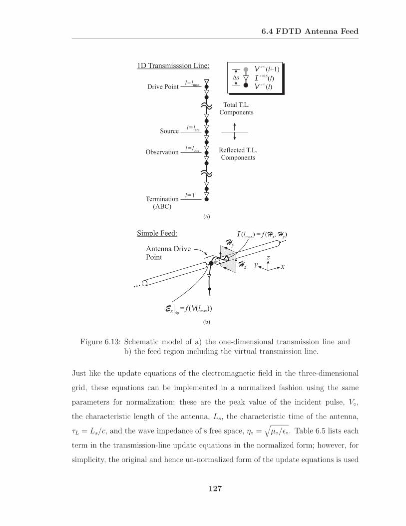
6.4 FDTD Antenna Feed
Antenna DrivePoint
…
…
xyz
Hy
Hz
Termination(ABC)
Source
Observation
V ( )n+1
l
V ( +1)n+1
l
I ( )n+0.5
ls
Drive Point
Reflected T.L.Components
Total T.L.Components
l l= max
l l= src
l l= obs
l=1
I ( ) = ( , )l fmax H Hx y
1D Transmisssion Line:
Simple Feed:
Ex = f l( ( ))V max
(a)
(b)
dp
Figure 6.13: Schematic model of a) the one-dimensional transmission line andb) the feed region including the virtual transmission line.
Just like the update equations of the electromagnetic field in the three-dimensional
grid, these equations can be implemented in a normalized fashion using the same
parameters for normalization; these are the peak value of the incident pulse, V,
the characteristic length of the antenna, Ls, the characteristic time of the antenna,
τL = Ls/c, and the wave impedance of s free space, η =√µ/ε. Table 6.5 lists each
term in the transmission-line update equations in the normalized form; however, for
simplicity, the original and hence un-normalized form of the update equations is used
127
6.4 FDTD Antenna Feed
Table 6.5: Normalization of the parameters in the transmission-line equations.
Original Parameter Normalized Parameter
V V/V
I I/(V/η)
c∆t/∆s (∆t/τL)/(∆s/Ls)
Zc Zc/η
throughout the remainder of this section.
The source excitation is established at the source plane within this transmission
line, see Fig. 6.13a, using the “one-way injector” [34, 45]. This non-physical source
implementation makes it possible to study the reflected voltage from the antenna
below the source plane without the superposition of the incident signal and is com-
monly referred to as one-way injector since the incident signal is launched at the
source plane in only one direction—towards the virtual drive point. Consequently,
the transmission-line components above the source plane at s = (lsrc− 1)∆s are total
voltages and total currents in the transmission-line equations, i.e., they contain the
incident and reflected components. The computational domain below and right at
this plane only contains the reflected transmission line components. For simplicity,
the voltages and currents in the line will be referenced either as total or reflected
components. The notation for the current is then
I =
Itot for l ≥ lsrc
Iref for l < lsrc
and for the voltage
V =
Vtot for l > lsrc
Vref for l ≤ lsrc.
For the transition between these two domains, one update equation for each compo-
nent (V and I) must be modified near the source plane by adding/subtracting the
128

6.4 FDTD Antenna Feed
time-domain expression of the excitation. Slightly modified updates for V and I re-sult for those update equations that contain mixed (total and reflected) components
in its original form, (6.47)-(6.48). The update for the current In+0.5(lsrc), right above
the source plane and therefore a total current is
In+0.5tot (lsrc) = In−0.5
tot (lsrc)− 1
Zc
c∆t
∆s
[Vntot(lsrc + 1)− Vn
tot(lsrc)]. (6.49)
However, the voltage Vntot(lsrc) observed right at the source plane is not a total voltage
but a reflected voltage in the transmission line. Since the total voltage is simply the
sum of incident and reflected voltage, i.e.,
Vntot(lsrc) = Vn
inc + Vnref(lsrc), (6.50)
(6.49) can be rewritten as
In+0.5tot (lsrc) = In−0.5
tot (lsrc)− 1
Zc
c∆t
∆s
[Vntot(lsrc + 1)− Vn
ref(lsrc)]
+1
Zc
c∆t
∆sVninc. (6.51)
Similarly, the modified update equation for the voltage right at the source plane can
be obtained, which must contain purely reflected transmission-line components, such
that (6.48) must be of the form
Vn+1ref (lsrc) = Vn
ref(lsrc)− Zcc∆t
∆s
[In+0.5ref (lsrc)− In+0.5
ref (lsrc − 1)]. (6.52)
However, the current I(lsrc) is a total current and must therefore be substituted bythe reflected component of the current
In+0.5ref (lsrc) = In+0.5
tot (lsrc)− In+0.5inc (lsrc)
= In+0.5tot (lsrc)− Vn+0.5
inc (s = (lsrc − 0.5)∆s)
Zc
. (6.53)
Note that the spatial offset of the incident voltage, determined ∆s/2 above the
source plane, must be converted into a temporal shift (delay), i.e., Vn+0.5inc (s = (lsrc −
129

6.4 FDTD Antenna Feed
0.5)∆s)) = Vinc(t = (n+0.5)∆t− 0.5∆s/c). Consequently, the final update equation
for the voltage at the source plane, can be written as
Vn+1ref (lsrc) = Vn
ref(lsrc)− Zcc∆t
∆s
[In+0.5tot (lsrc)− In+0.5
ref (lsrc − 1)]
+c∆t
∆sVn+0.5−0.5∆s/(c∆t)inc . (6.54)
A simple absorbing boundary condition is placed at the bottom end of the
transmission line. Note that for the Courant-Friedrichs-Levy (CFL) condition ∆t =
0.5∆s/c, the pulse propagates with velocity c one spatial step ∆s within two time
increments ∆t. For negligible reflection from the grid boundary, the first voltage in
this grid, V(1) must therefore be updated by the second voltage in this grid, V(2),observed two time steps earlier, i.e., Vn+1(1) = Vn−1(2).
To couple the transmission line to the three-dimensional FDTD grid and vice
versa, the line virtually attaches to the drive-point gap. Therefore, the voltage and
the current in the last cell are related to electric and magnetic fields in the vicinity of
the gap as shown schematically in Fig. 6.13b. To couple the line in the drive point,
the final voltage in the line is related to the tangential electric fields, that spread
across the gap between the antenna arms. In general, the voltage in the line and the
electric fields in the gap can be related using the line integral of the field across the
drive point, e.g., in the x direction,
V(lmax, t) = −∫gap
Ex dx. (6.55)
In the FDTD method, this integral can be broken up into summations to derive the
new update equations for the electric fields within the gap. As shown in Fig. 6.12 for
the drive point of the CSA, each electric field within the two-cell gap, that is marked
with a light gray line, is updated with
En+1x
∣∣∣dp= −Vn+1(lmax)
2∆x. (6.56)
To couple the drive point in the transmission line, the conduction current into
the antenna arm is related to the final current at the end of the transmission line,
130

6.4 FDTD Antenna Feed
In+0.5(lmax). This current can be expressed with a closed-path integral around the
conductor
I(lmax, t) =∮C&H · &ds. (6.57)
Ideally, the contour C should not include any displacement current but only a con-duction current. Therefore, the current contour should be shifted away from the gap
not to include any fringing of the field, which is explained in more detail in Appendix
B. As shown for the CSA in Fig. 6.12, the current contour consists of the magnetic
fields surrounding one sector of the feeding disc, that are marked with black lines and
thus determines the conduction current.
The apparent drive-point impedance [23] is determined using an approach that
involves both the incident and reflected voltage. Recall that the reflected voltage,
Vref , is observed at the plane with s = (lobs − 1)∆s, while the incident voltage Vincis injected at the source plane with s = (lsrc − 1)∆s, located above the observation
plane, shown qualitatively in Fig. 6.13a. Following basic transmission-line theory, the
input impedance can be determined using the reflection coefficient at the drive point
and the characteristic impedance of the line, i.e.,
Z(ω) = Zc1 + Γdp1− Γdp . (6.58)
This reflection coefficient, Γdp, can be written as the ratio of the reflected voltage and
the incident voltage provided both are observed at the same plane (drive point), i.e.,
Γdp(ω) =V dpref (ω)
V dpinc (ω)
=FVdp
ref(t)FVdp
inc(t). (6.59)
Notice, that the incident and reflected voltages are referenced to different planes well
beyond the drive point. In a straightforward approach, these voltages can easily be
transformed to the drive point. The reflected voltage, observed at the drive point,
Vdpref , is simply the time-advanced version of the reflected voltage at the observation
plane, Vref , that is
Vdpref(t) = Vref(t+ τobs) = Vref(t+ (lmax − lobs)∆s/c). (6.60)
131
6.5 Near-Field to Far-Field Transformer
Similarly, the observed incident voltage at the drive point, Vdpinc, is a time-delayed
version of the incident voltage at the source plane, Vinc, that is
Vdpinc(t) = Vinc(t− τsrc) = Vinc(t− (lmax − lsrc)∆s/c). (6.61)
These voltages can then be used to determine the reflection coefficient in (6.58)
Γdp(ω) =V dpref (ω)
V dpinc (ω)
=Vref(ω) e
−jωτobs
Vinc(ω) ejωτsrc=
Vref(ω)
Vinc(ω) ejω(τsrc+τobs). (6.62)
Instead of Fourier-transforming the original voltages, Vref(t) and Vinc(t), and subse-quently applying a phase shift, a slightly different approach is implemented in the
FDTD method that was shown to be more exact [41]. Notice that the denominator
term in (6.62), i.e., Vinc(ω) exp(jω(τsrc+ τobs)) or equivalently Vinc(t− (τsrc+ τobs)) in
the time domain, can be viewed as the (observed) incident voltage that propagated
the distance [(lmax − lobs) + (lmax − lsrc)]∆s in the transmission line, which is the
distance from the source plane to the drive point and back to the observation plane.
To avoid the shifts in the frequency domain and to account for spurious effects in
the transmission line, e.g., dispersion, this time-delayed voltage is determined in the
FDTD calculation using the following straightforward approach. By applying a short
circuit at the drive point with V(lmax) = 0, the reflected voltage at the observation
plane is
Vref |V(lmax)=0= −Vinc(t− (τsrc + τobs)), (6.63)
which, apart from the minus sign corresponds to the voltage in the denominator of
(6.62). This voltage can be determined concurrently within the same program that
is used to determine the antenna response and hence does not require additional
computational efforts.
6.5 Near-Field to Far-Field Transformer
Since the PML is truncating the FDTD lattice close to the antenna, only the field
in the space surrounding the antenna (near zone) is computed. However, often the
132

6.6 Program/Code Parallelization
field behavior at a large radial distance from the antenna (far zone) is of greater
interest. The electric field in the far zone of the CSA isolated in free space is obtained
with a near-field to far-field transformation based on Huygens’ Principle [31]. The
electric and magnetic field components tangential to the closed surface surrounding
the antenna, see Fig. 6.14, can be used to determine the radiated electric field in the
far zone of the antenna using a convolution integral:
&Er(&r, t) =µ4πr
∫∫S
r × r × ∂
∂t′[n× &H(&r ′, t′)
]
− 1
ηr × ∂
∂t′[n× &E(&r ′, t′)
]dS|t′=t−|%r−%r ′|/c. (6.64)
The primed variables, &r ′ and t′, denote the position and time for the fields observed
on the surface, while the unprimed variables, &r and t, refer to the position and time
for the fields observed in the far zone. The unit vector n is the outward normal to the
surface. The radiated field at the angle θ and at time t depends on the summation
of all tangential fields on the surface at the retarded times t − τi. The retardation
times τi = |&r − &r ′|/c are the times for a wave to propagate from the points on the
transforming box Qi to the far-field point P , as illustrated in Fig. 6.14.
6.6 Program/Code Parallelization
The solution space of a finite-difference model, especially for three-dimensional prob-
lems, can become quite large. Thus, in order to reduce the execution time of the simu-
lation, large parallel computers are commonly used. This section briefly lists common
parallel-computer architectures and outlines the code parallelization intended to take
full advantage of these architectures.
With Single-Process Multiple-Data (SPMD) multi processing (MP), multiple
CPUs execute a single program simultaneously. This approach can significantly in-
crease the performance11 and has been employed with great success on Unix supercom-
11Ideally, the execution time can be reduced by almost a factor of Np provided a parallel computer
133
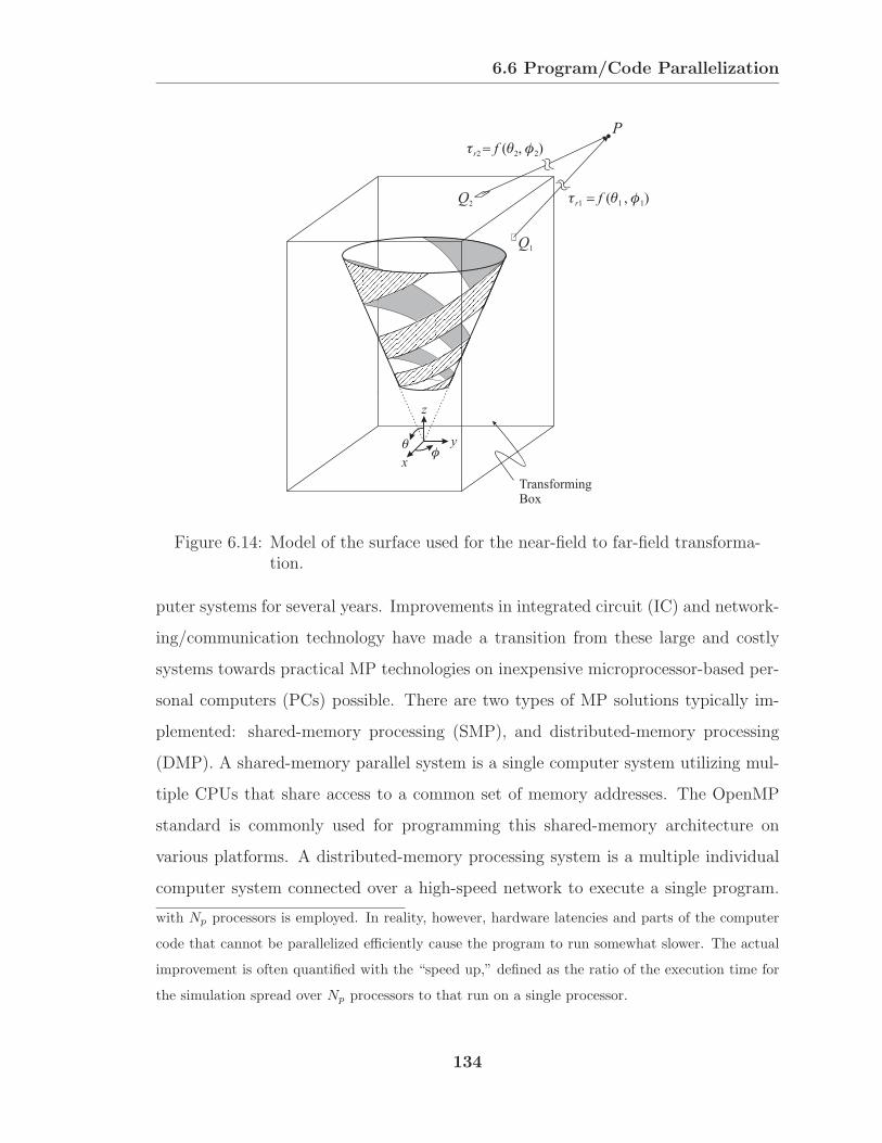
6.6 Program/Code Parallelization
TransformingBox
x
y
z
P
Q2
Q1
r2 2 2 f ( , )
r1 1 1 f ( , )
Figure 6.14: Model of the surface used for the near-field to far-field transforma-tion.
puter systems for several years. Improvements in integrated circuit (IC) and network-
ing/communication technology have made a transition from these large and costly
systems towards practical MP technologies on inexpensive microprocessor-based per-
sonal computers (PCs) possible. There are two types of MP solutions typically im-
plemented: shared-memory processing (SMP), and distributed-memory processing
(DMP). A shared-memory parallel system is a single computer system utilizing mul-
tiple CPUs that share access to a common set of memory addresses. The OpenMP
standard is commonly used for programming this shared-memory architecture on
various platforms. A distributed-memory processing system is a multiple individual
computer system connected over a high-speed network to execute a single program.
with Np processors is employed. In reality, however, hardware latencies and parts of the computer
code that cannot be parallelized efficiently cause the program to run somewhat slower. The actual
improvement is often quantified with the “speed up,” defined as the ratio of the execution time for
the simulation spread over Np processors to that run on a single processor.
134

6.6 Program/Code Parallelization
Subspace
Entire Solution Space Solution Space Dividedinto Subspaces
Figure 6.15: Division of the solution space into subspaces.
This approach has proven to be very successful dealing with extremely large problems
and has become popular within many research areas. The typical hardware config-
uration is a group of commodity computers connected via high-speed interconnects,
e.g., 100 Mbit/s Ethernet or Gigabit Ethernet. This configuration, dubbed as cluster
based computing or often referred to as “Beowulf cluster,” passes instructions and
data between systems via Message Passing Interface (MPI).
Figure 6.15 shows the basic parallelization scheme. In the conventional (serial)
three-dimensional finite-difference model, the transient fields are calculated through-
out the entire solution space by a single processor. To parallelize the finite-difference
model, the entire solution space is divided into several equal-sized subspaces. Each
subspace is assigned to one processor of the multi-processor architecture, which then
calculates the transient fields throughout its individual subspace.
At each time step, interface data must be exchanged between neighboring sub-
spaces, which is outlined in Fig. 6.16. Recall that one electric (magnetic) field com-
ponent at a discretized location in the grid depends on the difference of magnetic
(electric) field components in the immediate surrounding, i.e., four components in to-
tal. The fields located well inside the subspaces are independent of the fields in other
subspaces since the nearest neighbors are located in the same subspace. However,
the electric field located on the interface between two subspaces depends on at least
one magnetic field component from the neighboring subspaces, and the magnetic field
135

6.6 Program/Code Parallelization
in the immediate vicinity of such an interface depends on at least one electric field
component from neighboring subspaces. In the following, two examples are discussed
that require the exchange of information between two subspaces. In the first example,
illustrated in the top left corner in Fig. 6.16 for an interface with x = const, the elec-
tric field tangential to the interface between subspaces 1 and 2, Ex, depends on four
magnetic field components: Three of those are located entirely within the subspace 1,
while the fourth magnetic field, Hz, is located in subspace 2. In the second example,
illustrated in the top right corner of Fig. 6.16 for an interface with x = const, the
magnetic field component, Hz, in subspace 2 right next to the interface depends on
four electric field components: Three of those are located within subspace 2, while the
remaining electric field, Ex, belongs to subspace 1 (even though it is located on the
shared interface). Therefore, it is necessary to pass the interface data of the electric
field right at the interface and that of the magnetic field right next to the interface
from one subspace to its immediate neighbor, as shown in the bottom of Fig. 6.16.
As part of the research for this dissertation, a Fortran90 computer code was par-
allelized using both the shared-memory approach (using OpenMP) and the message-
passing approach (using MPI). Initially, the OpenMP program was executed on a
SMP architecture, i.e., a Dell Poweredge Quad Pentium III-Xeon (500 MHz) server
with 2 GB RAM. Later, the program was rewritten using the MPI approach to run
simulations on both SMP and DMP architectures. The latter was a Beowulf cluster
with 50 Pentium III (500 MHz) processors and a total of 6 GB RAM, interconnected
via FastEthernet (100 Mbit/s).
To parallelize an already existing serial version of the Fortran90 program, al-
most all subroutines needed to be modified to operate on the corresponding subspace
instead of the entire domain. Therefore, the following MPI commands were essen-
tial [46], such as MPI INIT, MPI COMM RANK, MPI COMM SIZE, MPI SEND, MPI RECEIVE,
MPI BARRIER, and MPI FINALIZE.12
12Within an MPI environment enclosed by MPI INIT and MPI FINALIZE, a user defined number
of processes are created. In the current implementation, each process updates the electromagnetic
136
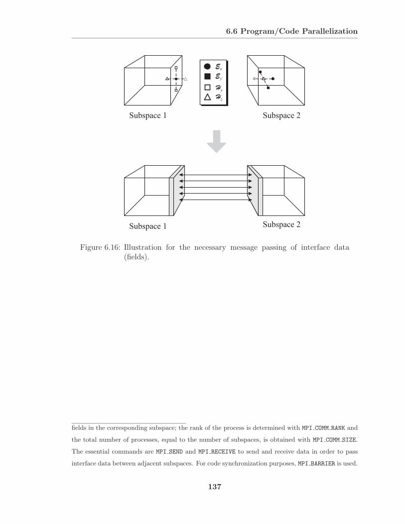
6.6 Program/Code Parallelization
Subspace 1 Subspace 2
Subspace 1 Subspace 2
Hz
Ex
Ey
Hy
Figure 6.16: Illustration for the necessary message passing of interface data(fields).
fields in the corresponding subspace; the rank of the process is determined with MPI COMM RANK and
the total number of processes, equal to the number of subspaces, is obtained with MPI COMM SIZE.
The essential commands are MPI SEND and MPI RECEIVE to send and receive data in order to pass
interface data between adjacent subspaces. For code synchronization purposes, MPI BARRIER is used.
137

CHAPTER 7
Validation of FDTD Results
This chapter is concerned with the validation of the FDTD method used to model the
CSA in free space and over ground. In Section 7.1, numerical results are compared
with results published in the literature. First, results obtained for an unloaded CSA
and a CSA terminated with lumped resistors are compared with measurements made
elsewhere. Then, results obtained for linear dipole antennas placed horizontally over
lossy media are compared with analytical and experimental results of others. In
Section 7.2, measurements performed at Georgia Tech are described. The fabrication
of the CSA, the feed system, and the measurement techniques for the input impedance
and the realized gain are explained.
7.1 Validation using Published Results
7.1.1 CSA in Free Space
In this section, measurements performed by Ramsdale [17] for the input impedance
and the electric field in the far zone of the CSA are compared with numerical results
obtained using the FDTD method. The results presented here are for a right-handed
CSA with the following parameters: θ = 15, α = 60, δ = 90, and D/d = 12.77
with D = 15.2 cm. The antenna is fed from a transmission line with the characteristic
impedance Zc = 100Ω. The results are for the unloaded CSA and the CSA termi-
nated with lumped resistors. Each of the lumped resistors, connected in parallel at
138

7.1 Validation using Published Results
the closest edges of the two arms, has a resistance of RL = 300Ω. For the FDTD cal-
culations, the dimensions of the cells are ∆x = ∆y = ∆z ≈ 1.2mm; this corresponds
to a discretization of 125 cells per wavelength at the highest frequency studied.
The reflection coefficient is plotted on a Smith chart in Fig. 7.1a for the unloaded
antenna and in Fig. 7.1b for the loaded antenna. The FDTD results are plotted with
a black line, the measurements are plotted with a gray line. Points are marked that
correspond to a reflection coefficient at particular frequencies. For low frequencies,
the reflection coefficient for the unloaded antenna agrees well with the measurements,
while some deviations can be seen for higher frequencies. Since high frequencies/short
wavelengths are radiated from the small end of the CSA, these deviations probably
result from the differences in the feed system. The modeling of the feed in the exper-
imental model and in the numerical model are indeed different. In the experimental
model, two rigid coaxial lines are attached to the feed point at the disc, while in
the FDTD model a two-wire transmission line is connected to these feed points, as
outlined in Section 6.4. For the loaded case, both curves show that the reflections are
centered in a small region about the point R/Zc = 1.5. Although the shapes of the
reflection coefficient curves are different, both curves circle around the same point,
which corresponds to an impedance of 150Ω. As stated earlier, the end termination
should not affect the high frequencies significantly. This behavior can be seen in the
numerical results for the reflection coefficient, since both curves look similar in the
high-frequency range.
In Fig. 7.2, vertical-plane (φ = 90), far-zone patterns are shown for the fre-
quency f = 0.5GHz. The patterns, graphed on a logarithmic scale, are given for
both of the circularly polarized components of the electric field for the unloaded CSA
in Fig. 7.2a and for the loaded CSA in Fig. 7.2b. The numerical results for the
left-handed circularly polarized component of the electric field, ErLHCP, are shown
with a dotted line using hollow dots, and those for the right-handed circularly polar-
ized component of the field, ErRHCP, are shown with a dotted line using solid dots.
The corresponding experimental results are shown with a solid line. The agreement
139
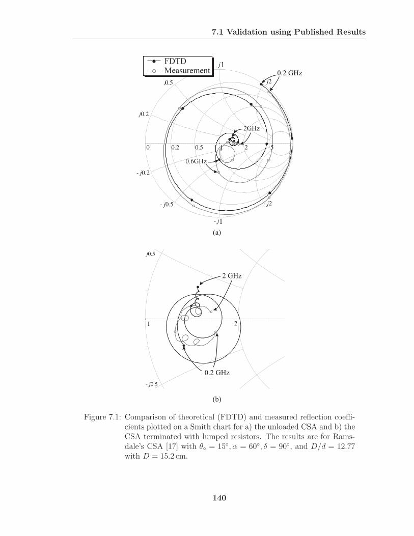
7.1 Validation using Published Results
0.2 GHz
2GHz
0.6GHz
0.2 GHz
2 GHz
(a)
(b)
FDTDMeasurement
1
1
Figure 7.1: Comparison of theoretical (FDTD) and measured reflection coeffi-cients plotted on a Smith chart for a) the unloaded CSA and b) theCSA terminated with lumped resistors. The results are for Rams-dale’s CSA [17] with θ = 15, α = 60, δ = 90, and D/d = 12.77with D = 15.2 cm.
140

7.1 Validation using Published Results
-30 -20 -10 0
-30
-20
-10
0
-30-20-100
-30
-20
-10
0
0
30
60
90
120
150
180
210
240
270
300
330
-30 -20 -10 0
-30
-20
-10
0
-30-20-100
-30
-20
-10
0
0
30
60
90
120
150
180
210
240
270
300
330
(a)
(b)
E
ER
L
(FDTD)
(FDTD)
Measurement
dB
dB
Figure 7.2: Comparison of theoretical (FDTD) and measured far zone patternsfor the circularly polarized components of the electric field for a) theunloaded CSA and b) the CSA terminated with lumped resistors(RL = 300Ω) at f = 0.5GHz. The results are for Ramsdale’sCSA [17] with θ = 15, α = 60, δ = 90, and D/d = 12.77 withD = 15.2 cm.
141
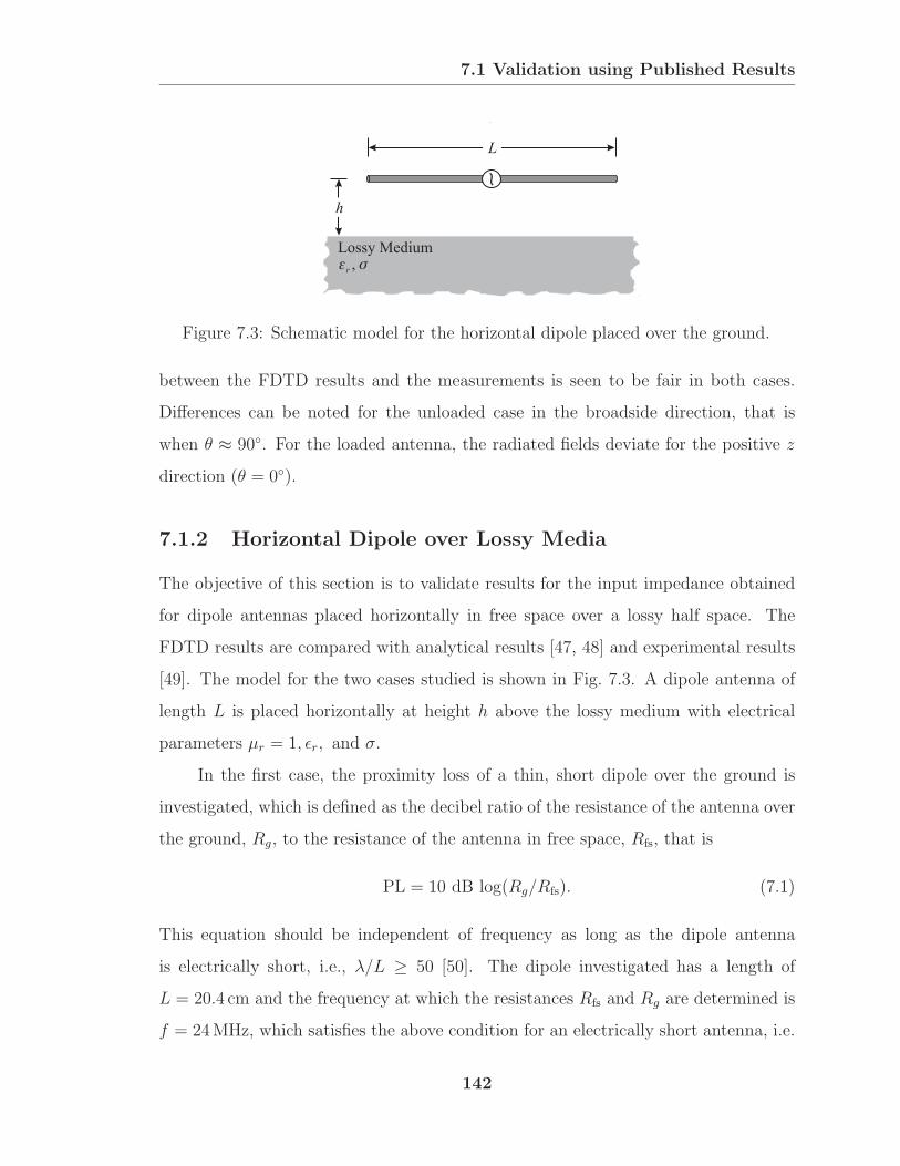
7.1 Validation using Published Results
r ,
h
L
Lossy Medium
Figure 7.3: Schematic model for the horizontal dipole placed over the ground.
between the FDTD results and the measurements is seen to be fair in both cases.
Differences can be noted for the unloaded case in the broadside direction, that is
when θ ≈ 90. For the loaded antenna, the radiated fields deviate for the positive z
direction (θ = 0).
7.1.2 Horizontal Dipole over Lossy Media
The objective of this section is to validate results for the input impedance obtained
for dipole antennas placed horizontally in free space over a lossy half space. The
FDTD results are compared with analytical results [47, 48] and experimental results
[49]. The model for the two cases studied is shown in Fig. 7.3. A dipole antenna of
length L is placed horizontally at height h above the lossy medium with electrical
parameters µr = 1, εr, and σ.
In the first case, the proximity loss of a thin, short dipole over the ground is
investigated, which is defined as the decibel ratio of the resistance of the antenna over
the ground, Rg, to the resistance of the antenna in free space, Rfs, that is
PL = 10 dB log(Rg/Rfs). (7.1)
This equation should be independent of frequency as long as the dipole antenna
is electrically short, i.e., λ/L ≥ 50 [50]. The dipole investigated has a length of
L = 20.4 cm and the frequency at which the resistances Rfs and Rg are determined is
f = 24MHz, which satisfies the above condition for an electrically short antenna, i.e.
142
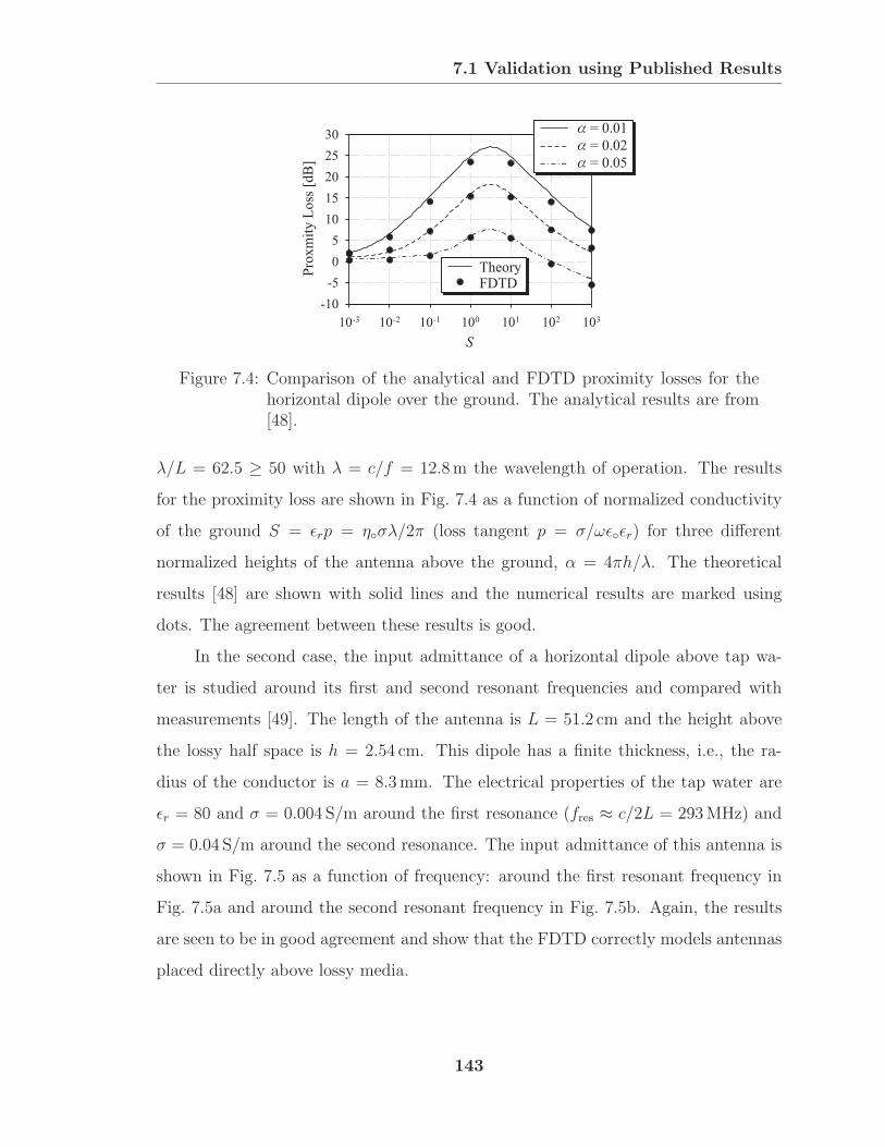
7.1 Validation using Published Results
10-3 10-2 10-1 100 101 102 103
-10
-5
0
5
10
15
20
25
30
S
Pro
xm
ity
Loss
[dB
]
= 0.01
= 0.02
= 0.05
TheoryFDTD
Figure 7.4: Comparison of the analytical and FDTD proximity losses for thehorizontal dipole over the ground. The analytical results are from[48].
λ/L = 62.5 ≥ 50 with λ = c/f = 12.8m the wavelength of operation. The results
for the proximity loss are shown in Fig. 7.4 as a function of normalized conductivity
of the ground S = εrp = ησλ/2π (loss tangent p = σ/ωεεr) for three different
normalized heights of the antenna above the ground, α = 4πh/λ. The theoretical
results [48] are shown with solid lines and the numerical results are marked using
dots. The agreement between these results is good.
In the second case, the input admittance of a horizontal dipole above tap wa-
ter is studied around its first and second resonant frequencies and compared with
measurements [49]. The length of the antenna is L = 51.2 cm and the height above
the lossy half space is h = 2.54 cm. This dipole has a finite thickness, i.e., the ra-
dius of the conductor is a = 8.3mm. The electrical properties of the tap water are
εr = 80 and σ = 0.004 S/m around the first resonance (fres ≈ c/2L = 293MHz) and
σ = 0.04 S/m around the second resonance. The input admittance of this antenna is
shown in Fig. 7.5 as a function of frequency: around the first resonant frequency in
Fig. 7.5a and around the second resonant frequency in Fig. 7.5b. Again, the results
are seen to be in good agreement and show that the FDTD correctly models antennas
placed directly above lossy media.
143
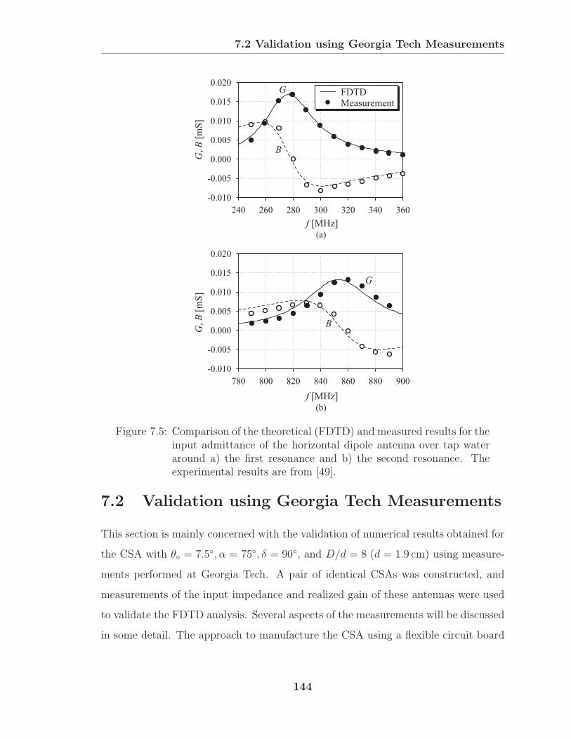
7.2 Validation using Georgia Tech Measurements
240 260 280 300 320 340 360
-0.010
-0.005
0.000
0.005
0.010
0.015
0.020
f [MHz]
f [MHz]
GB
,[m
S]
GB
,[m
S]
B
G FDTDMeasurement
780 800 820 840 860 880 900
-0.010
-0.005
0.000
0.005
0.010
0.015
0.020
B
G
(a)
(b)
Figure 7.5: Comparison of the theoretical (FDTD) and measured results for theinput admittance of the horizontal dipole antenna over tap wateraround a) the first resonance and b) the second resonance. Theexperimental results are from [49].
7.2 Validation using Georgia Tech Measurements
This section is mainly concerned with the validation of numerical results obtained for
the CSA with θ = 7.5, α = 75, δ = 90, and D/d = 8 (d = 1.9 cm) using measure-
ments performed at Georgia Tech. A pair of identical CSAs was constructed, and
measurements of the input impedance and realized gain of these antennas were used
to validate the FDTD analysis. Several aspects of the measurements will be discussed
in some detail. The approach to manufacture the CSA using a flexible circuit board
144

7.2 Validation using Georgia Tech Measurements
material is explained in Section 7.2.1. The antenna feeding technique together with
the experimental validation of the balun are presented in Section 7.2.2. In Section
7.2.3, the experimental implementations of the resistive terminations (lumped resis-
tors and the resistive sheet) are discussed, and each termination is examined with
separate measurements. The measurement for the input impedance is explained in
Section 7.2.4, while the two-port measurement for the realized gain is explained in
Section 7.2.5. In Section 7.2.6, the same two-port measurement technique is used to
determine the input impedance, realized gain, and gain for a dipole antenna. These
results are then compared to numerical results obtained with the FDTD method.
7.2.1 Manufacturing of the CSA
The objective for the CSA design was to build and measure a CSA with performance
characteristics such as uniform impedance, unidirectional radiation, and circular po-
larization over a broad range of frequencies, that are beneficial for applications when
isolated in free space or placed over the ground. Therefore, CSAs with small half-cone
angles, θ, and large wrap angles, α, were of main interest; thus, the characteristic
angles of the antenna were chosen to be θ = 7.5, α = 75, and δ = 90. The re-
maining parameters d = 1.9 cm and D/d = 8 were chosen for practical reasons. The
small end is where the CSA is fed, the smallest diameter must therefore be sufficiently
big to fit the feed cables and the connectors that attach to the feeding end of the
antenna. The ratio of biggest to smallest diameter, D/d = 8, guaranteed that the
CSA would just fit on the biggest available flexible circuit-board sheet that measured
43.2 cm× 58.4 cm (17′′ × 23′′).The general approach for fabricating the CSA is to form the metallic spiral arms
on a flexible circuit board by etching away the unwanted portion of the coating.
The circuit board is then wrapped around a solid conical mandrel, and the arms
are soldered together along the seam. This manufacturing of the CSA requires the
proper design of the planar sheet that when wrapped on a cone becomes the CSA.
145

7.2 Validation using Georgia Tech Measurements
Figure 7.6: Illustration on how the conical surface becomes a circular sectorand vice versa.
Figure 7.6 illustrates that by unwrapping the conical surface on a plane a sector is
obtained that has circular arcs at the small and the big end. Schematic drawings for
this planar surface are shown in Fig. 7.7. Simple geometry can be used to show that
the maximum dimensions of the sector are its height
Ys =
D sin(2π sin θ)2 sin θ for θ ≤ 14.5
2D for 14.5 < θ ≤ 30(7.2)
and its width
Xs =
D2 sin θ −
d cos(2π sin θ)2 sin θ for θ ≤ 14.5
2D[1− cos(2π sin θ)] for 14.5 < θ ≤ 30. (7.3)
Note that these equations must be determined separately for different ranges of θ, i.e.,
each time the angular width of the sector, β = 2π sin θ, exceeds an integer multiple
of 90. Here, just the results for the most common ranges of θ are presented, as
illustrated in Fig. 7.7.
In the next step, the boundaries of the metallic arms must be transferred on
the planar surface using simple geometrical expressions. The template for the copper
etching process of the unwrapped CSA with θ = 7.5, α = 75, δ = 90, and D/d = 8
is shown in Fig. 7.8a. Here, the two antenna arms are shown in two different shades
of gray. When this model is wrapped around a conical mandrel, the arms properly
connect at the seam, as illustrated in the inset of Fig. 7.8a. For the actual manu-
facturing process, the boundary information of the arms was stored in a Gerber1 file
format, and the arms were then formed on a flexible circuit board material through a
1The Gerber format is used primarily by designers who need to make format checkplots of PC
146
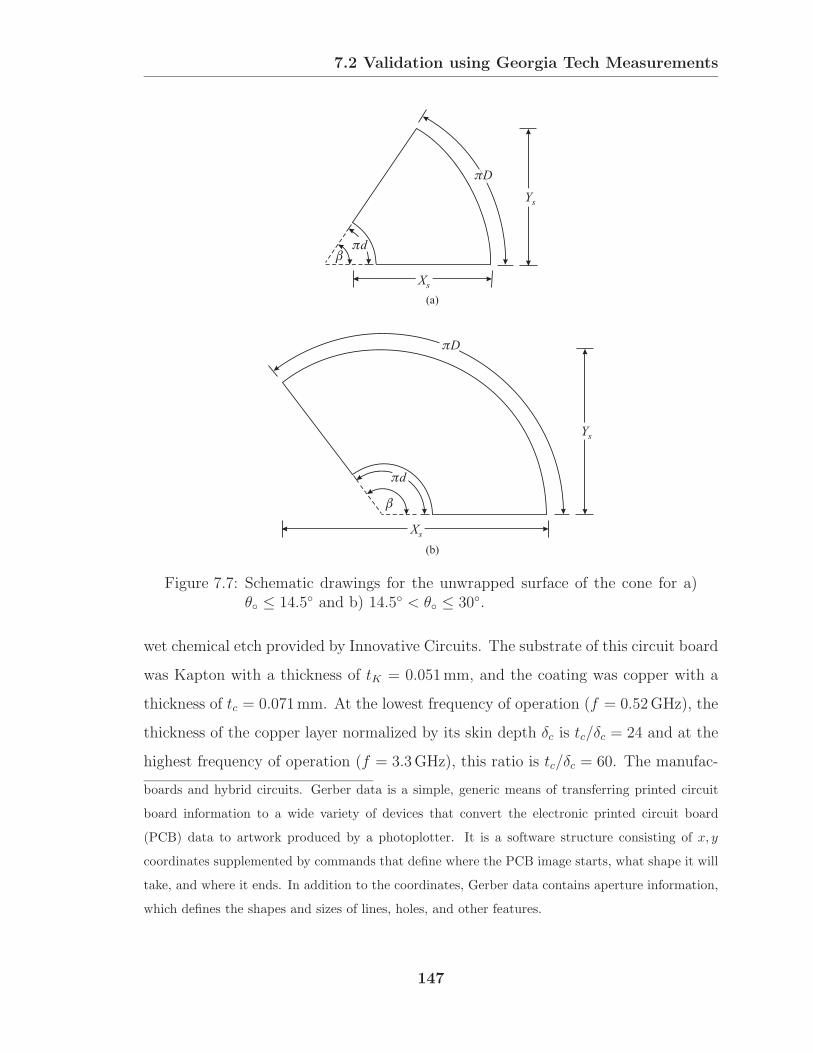
7.2 Validation using Georgia Tech Measurements
d
D
Ys
Xs
d
Ys
Xs
D
(a)
(b)
Figure 7.7: Schematic drawings for the unwrapped surface of the cone for a)θ ≤ 14.5 and b) 14.5 < θ ≤ 30.
wet chemical etch provided by Innovative Circuits. The substrate of this circuit board
was Kapton with a thickness of tK = 0.051mm, and the coating was copper with a
thickness of tc = 0.071mm. At the lowest frequency of operation (f = 0.52GHz), the
thickness of the copper layer normalized by its skin depth δc is tc/δc = 24 and at the
highest frequency of operation (f = 3.3GHz), this ratio is tc/δc = 60. The manufac-
boards and hybrid circuits. Gerber data is a simple, generic means of transferring printed circuit
board information to a wide variety of devices that convert the electronic printed circuit board
(PCB) data to artwork produced by a photoplotter. It is a software structure consisting of x, y
coordinates supplemented by commands that define where the PCB image starts, what shape it will
take, and where it ends. In addition to the coordinates, Gerber data contains aperture information,
which defines the shapes and sizes of lines, holes, and other features.
147

7.2 Validation using Georgia Tech Measurements
Kapton(Substrate)
Copper (Coating),Metallic Arms
(a)
(b)
Figure 7.8: a) Template for the copper etching process, b) photograph of themanufactured flexible circuit board.
tured flexible circuit board with the spiral arms formed on the surface is shown in a
photograph in Fig. 7.8b.
Next, the planar surface must take on the shape of the conical surface. First,
small patches of solder were placed on the metallic (copper) regions along the sides
of the planar circuit board, as shown in Fig. 7.9a. Then, the surface was wrapped
148

7.2 Validation using Georgia Tech Measurements
around a conical mandrel and the spiral arms were soldered together at the seam.
This was done by soldering small patches of brass sheet on each previously prepared
end of the spiral arm. The assembled CSA is shown in Fig. 7.9b.
7.2.2 Feed System of the CSA
The following section is concerned with the antenna feed system used for the CSA
measurements. The feeding technique consists of three main components: the feeding
disc at the small end of the CSA, the feed cable running along the axis of the antenna,
and the balun that is placed in between the feed cable and the vector network analyzer.
These components are illustrated schematically in Fig. 7.10.
The details of the feed point of the antenna are shown at the top of Fig. 7.10.
The small disc of rigid circuit board contained two symmetric angular sectors of
conductor. The disc just fits into the open end of the CSA. Holes were drilled into
each metallic sector, into which metallic pins were soldered. The pins protruded into
the cone. The feeding disc used in the measurements is shown in Fig. 7.11a with
and without the pins attached. The metallic sectors of the feeding disc were put in
electrical contact with the two arms of the CSA by soldering both metallic regions
together using brass sheets, see Fig. 7.11b.
A pair of semi-rigid coaxial lines (Zc = 50Ω) ran along the axis of the cone.
After leaving the balun, these lines were electrically bonded together to suppress
unbalanced modes, i.e., currents on the surface of the coaxial lines. The lines did not
separate again until they reached the feed point. Female connectors were soldered to
the ends of these lines, and the pins on the arms of the antenna were inserted into the
center conductors of these connectors to temporarily attach the antenna to the feed
cables. The network analyzer was calibrated by connecting standard terminations
(matched load, short circuit, and open circuit) simultaneously to both of the female
connectors. Thus, the plane for calibration of the measurement was right at the
terminals of the antenna.
149
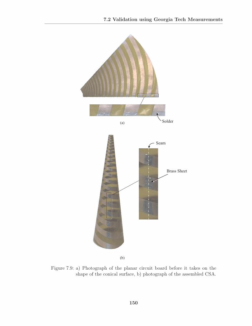
7.2 Validation using Georgia Tech Measurements
(a)
(b)
Brass Sheet
Seam
Solder
Figure 7.9: a) Photograph of the planar circuit board before it takes on theshape of the conical surface, b) photograph of the assembled CSA.
150
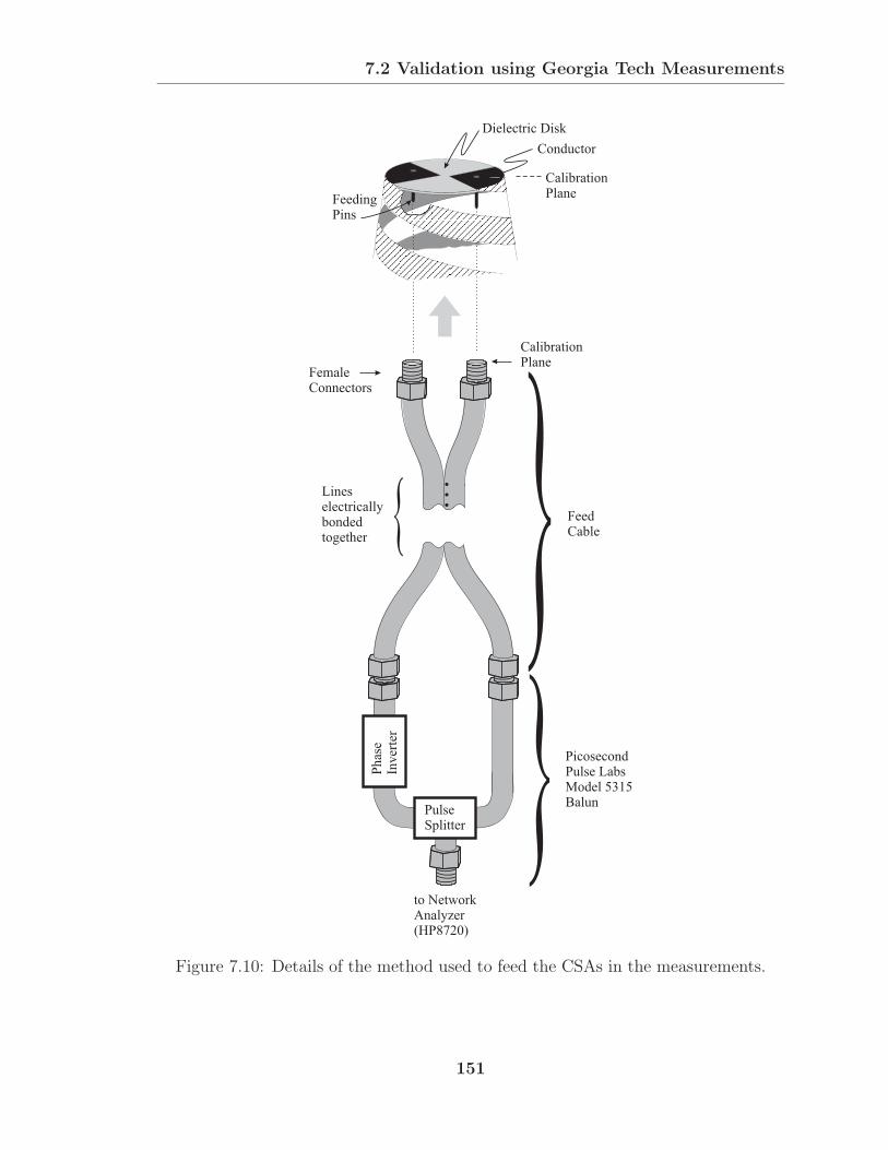
7.2 Validation using Georgia Tech Measurements
CalibrationPlane
CalibrationPlane
Conductor
Dielectric Disk
to NetworkAnalyzer(HP8720)
FeedCable
PicosecondPulse LabsModel 5315Balun
PulseSplitter
Phas
eIn
ver
ter
FeedingPins
…
FemaleConnectors
Lineselectricallybondedtogether
Figure 7.10: Details of the method used to feed the CSAs in the measurements.
151

7.2 Validation using Georgia Tech Measurements
(a)
(b)
Figure 7.11: a) Photograph of the rigid circuit board used to connect the feedcable with the antenna arms, b) photograph of the feed region.
The CSA is a balanced structure, and the measurements to be described were
made using a vector network analyzer (HP8720) with coaxial ports (unbalanced), see
Fig. 7.12a for a photograph. Therefore, a balun had to be used with each antenna.
The balun selected was the Picosecond Pulse Labs Model 5315, see the bottom of
Fig. 7.10 and Fig. 7.12b for a photograph. All ports of the balun had the characteristic
impedance Zc = 50Ω, so the balun can be used to effectively connect an unbalanced
line with Zc = 50Ω to a balanced line with Zc = 100Ω. The balun was located well
outside the antenna so as to not affect the performance of the antenna.
The balun was examined quantitatively using the measurement setup shown in
Fig. 7.13. Three separate two-port measurements were performed to determine the
insertion loss of each combination of ports and the return loss of the three ports.
These measurements were also used to verify that the two output ports are 180 out
of phase. In each of the experiments, two ports i and j of the balun were connected
152
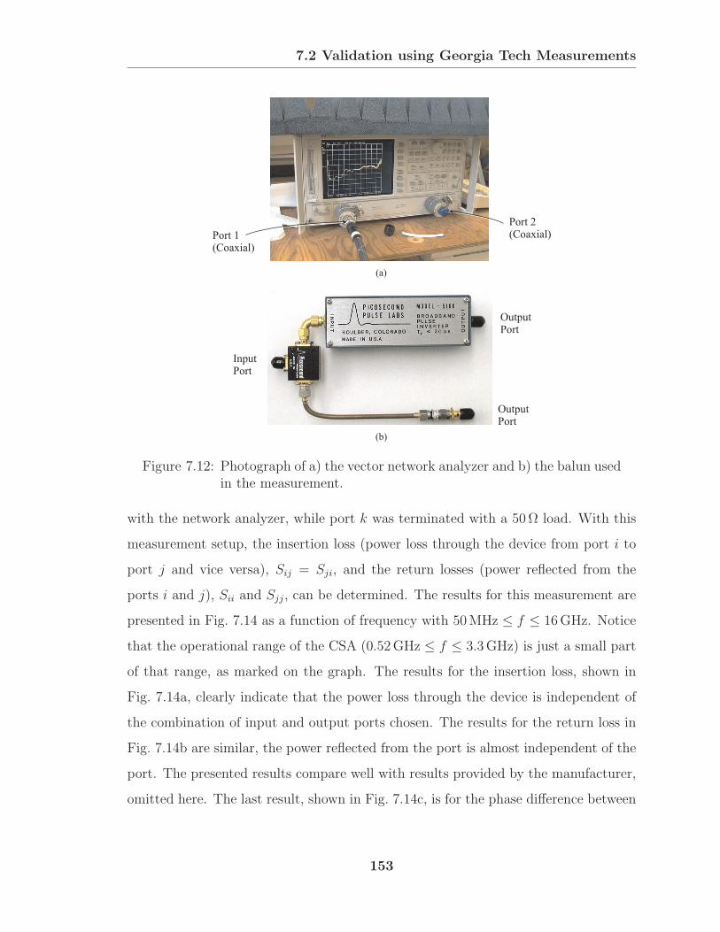
7.2 Validation using Georgia Tech Measurements
(a)
(b)
Port 1(Coaxial)
Port 2(Coaxial)
OutputPort
OutputPort
InputPort
Figure 7.12: Photograph of a) the vector network analyzer and b) the balun usedin the measurement.
with the network analyzer, while port k was terminated with a 50Ω load. With this
measurement setup, the insertion loss (power loss through the device from port i to
port j and vice versa), Sij = Sji, and the return losses (power reflected from the
ports i and j), Sii and Sjj, can be determined. The results for this measurement are
presented in Fig. 7.14 as a function of frequency with 50MHz ≤ f ≤ 16GHz. Notice
that the operational range of the CSA (0.52GHz ≤ f ≤ 3.3GHz) is just a small part
of that range, as marked on the graph. The results for the insertion loss, shown in
Fig. 7.14a, clearly indicate that the power loss through the device is independent of
the combination of input and output ports chosen. The results for the return loss in
Fig. 7.14b are similar, the power reflected from the port is almost independent of the
port. The presented results compare well with results provided by the manufacturer,
omitted here. The last result, shown in Fig. 7.14c, is for the phase difference between
153

7.2 Validation using Georgia Tech Measurements
50
`
1
2
3
50
To VNA(Port #2)
To VNA(Port #1)
(a)
1
2
3
50
To VNA(Port #2)
To VNA(Port #1)
(b)
1
2
3
To VNA(Port #2)
To VNA(Port #1)
(c)
Figure 7.13: Schematic drawings for the two-port measurements of the balun:a) is for determining S11, S12, S21, and S22, b) for S11, S13, S31, andS33, and c) for S22, S23, S32, and S33.
154
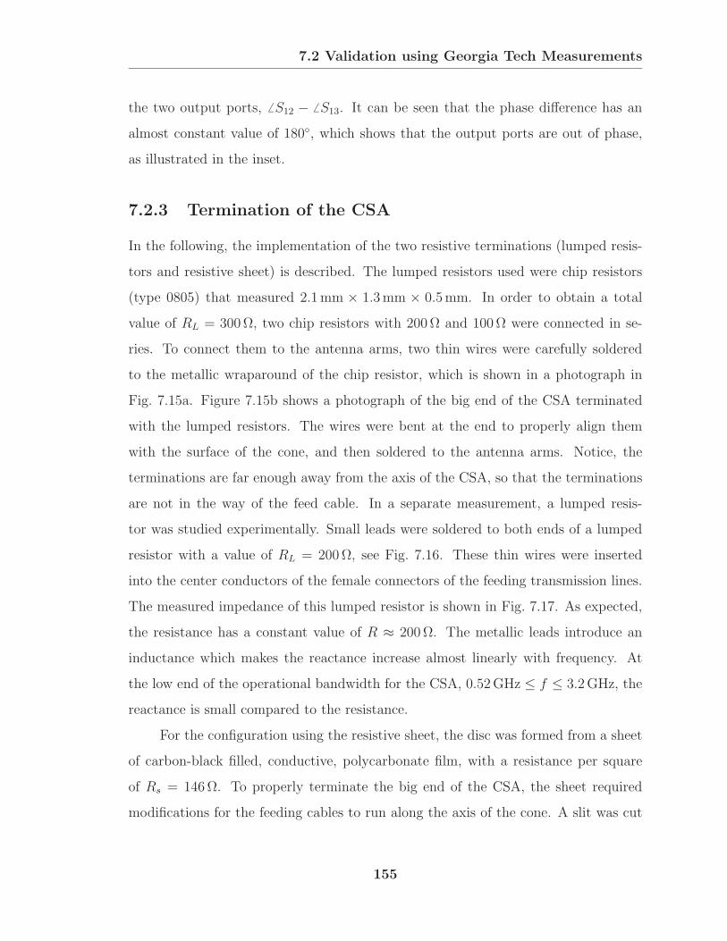
7.2 Validation using Georgia Tech Measurements
the two output ports, S12 − S13. It can be seen that the phase difference has an
almost constant value of 180, which shows that the output ports are out of phase,
as illustrated in the inset.
7.2.3 Termination of the CSA
In the following, the implementation of the two resistive terminations (lumped resis-
tors and resistive sheet) is described. The lumped resistors used were chip resistors
(type 0805) that measured 2.1mm × 1.3mm × 0.5mm. In order to obtain a total
value of RL = 300Ω, two chip resistors with 200Ω and 100Ω were connected in se-
ries. To connect them to the antenna arms, two thin wires were carefully soldered
to the metallic wraparound of the chip resistor, which is shown in a photograph in
Fig. 7.15a. Figure 7.15b shows a photograph of the big end of the CSA terminated
with the lumped resistors. The wires were bent at the end to properly align them
with the surface of the cone, and then soldered to the antenna arms. Notice, the
terminations are far enough away from the axis of the CSA, so that the terminations
are not in the way of the feed cable. In a separate measurement, a lumped resis-
tor was studied experimentally. Small leads were soldered to both ends of a lumped
resistor with a value of RL = 200Ω, see Fig. 7.16. These thin wires were inserted
into the center conductors of the female connectors of the feeding transmission lines.
The measured impedance of this lumped resistor is shown in Fig. 7.17. As expected,
the resistance has a constant value of R ≈ 200Ω. The metallic leads introduce an
inductance which makes the reactance increase almost linearly with frequency. At
the low end of the operational bandwidth for the CSA, 0.52GHz ≤ f ≤ 3.2GHz, the
reactance is small compared to the resistance.
For the configuration using the resistive sheet, the disc was formed from a sheet
of carbon-black filled, conductive, polycarbonate film, with a resistance per square
of Rs = 146Ω. To properly terminate the big end of the CSA, the sheet required
modifications for the feeding cables to run along the axis of the cone. A slit was cut
155

7.2 Validation using Georgia Tech Measurements
0.05 2 4 6 8 10 12 14 16
0.0
0.2
0.4
0.6
0.8
1.0
0.05 2 4 6 8 10 12 14 16
0.0
0.2
0.4
0.6
0.8
1.0
0.05 2 4 6 8 10 12 14 16
-225
-180
-135
-90
-45
0
Inse
rtio
nL
oss
Ret
urn
Lo
ss
f [GHz]
f [GHz]
f [GHz]
(a)
(b)
(c)
| |
| |
| |
S
S
S
12
13
23
| |
| |
| |
S
S
S
11
22
33
SS
12
13
-
1
2
3
Frequency Range for CSA
Figure 7.14: Measured results for the a) insertion loss, b) return loss, and c)phase difference between the output ports.
156

7.2 Validation using Georgia Tech Measurements
(a)
(b)
Chip Resistor
Figure 7.15: Photograph of a) the lumped resistor termination (chip resistor sol-dered to the wires) and b) the big end of the CSA when terminatedwith lumped resistors.
FeedCable
…
RL = 200
Figure 7.16: Schematic drawing for the measurement of the lumped resistor.
157
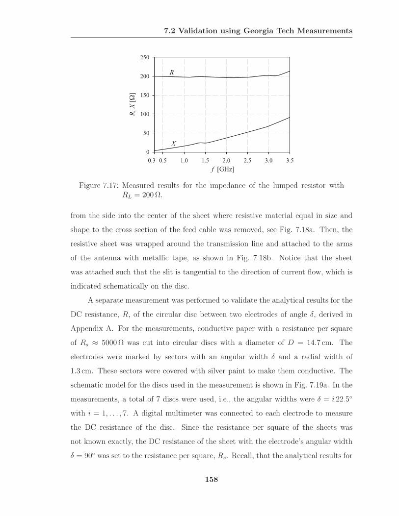
7.2 Validation using Georgia Tech Measurements
0.3 0.5 1.0 1.5 2.0 2.5 3.0 3.5
0
50
100
150
200
250
f [GHz]
R,X
[]
R
X
Figure 7.17: Measured results for the impedance of the lumped resistor withRL = 200Ω.
from the side into the center of the sheet where resistive material equal in size and
shape to the cross section of the feed cable was removed, see Fig. 7.18a. Then, the
resistive sheet was wrapped around the transmission line and attached to the arms
of the antenna with metallic tape, as shown in Fig. 7.18b. Notice that the sheet
was attached such that the slit is tangential to the direction of current flow, which is
indicated schematically on the disc.
A separate measurement was performed to validate the analytical results for the
DC resistance, R, of the circular disc between two electrodes of angle δ, derived in
Appendix A. For the measurements, conductive paper with a resistance per square
of Rs ≈ 5000Ω was cut into circular discs with a diameter of D = 14.7 cm. The
electrodes were marked by sectors with an angular width δ and a radial width of
1.3 cm. These sectors were covered with silver paint to make them conductive. The
schematic model for the discs used in the measurement is shown in Fig. 7.19a. In the
measurements, a total of 7 discs were used, i.e., the angular widths were δ = i 22.5
with i = 1, . . . , 7. A digital multimeter was connected to each electrode to measure
the DC resistance of the disc. Since the resistance per square of the sheets was
not known exactly, the DC resistance of the sheet with the electrode’s angular width
δ = 90 was set to the resistance per square, Rs. Recall, that the analytical results for
158
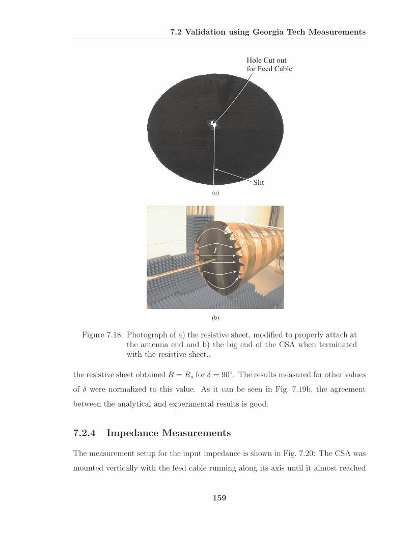
7.2 Validation using Georgia Tech Measurements
(a)
(b)
Hole Cut outfor Feed Cable
Slit
I
Figure 7.18: Photograph of a) the resistive sheet, modified to properly attach atthe antenna end and b) the big end of the CSA when terminatedwith the resistive sheet..
the resistive sheet obtained R = Rs for δ = 90. The results measured for other values
of δ were normalized to this value. As it can be seen in Fig. 7.19b, the agreement
between the analytical and experimental results is good.
7.2.4 Impedance Measurements
The measurement setup for the input impedance is shown in Fig. 7.20: The CSA was
mounted vertically with the feed cable running along its axis until it almost reached
159
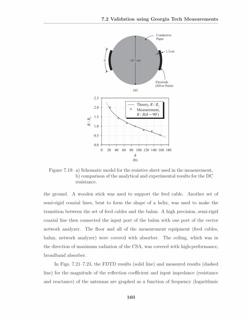
7.2 Validation using Georgia Tech Measurements
14.7 cm
1.3cm
ConductivePaper
Electrode(Silver Paint)
0 20 40 60 80 100 120 140 160 180
0.0
0.5
1.0
1.5
2.0
2.5
RR
/s
(a)
(b)
Theory, /
Measurement,
R Rs
R R/ ( = 90 )o
……
Figure 7.19: a) Schematic model for the resistive sheet used in the measurement,b) comparison of the analytical and experimental results for the DCresistance.
the ground. A wooden stick was used to support the feed cable. Another set of
semi-rigid coaxial lines, bent to form the shape of a helix, was used to make the
transition between the set of feed cables and the balun. A high precision, semi-rigid
coaxial line then connected the input port of the balun with one port of the vector
network analyzer. The floor and all of the measurement equipment (feed cables,
balun, network analyzer) were covered with absorber. The ceiling, which was in
the direction of maximum radiation of the CSA, was covered with high-performance,
broadband absorber.
In Figs. 7.21–7.23, the FDTD results (solid line) and measured results (dashed
line) for the magnitude of the reflection coefficient and input impedance (resistance
and reactance) of the antennas are graphed as a function of frequency (logarithmic
160
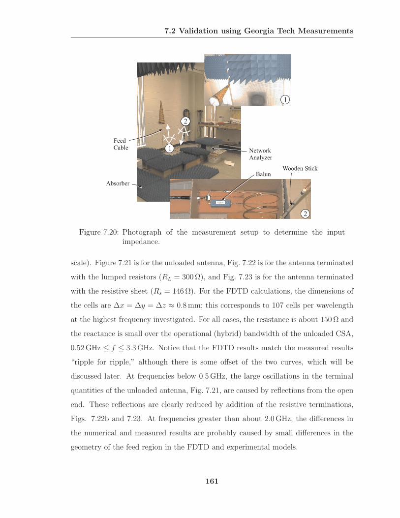
7.2 Validation using Georgia Tech Measurements
1
1
2
2
Absorber
FeedCable
NetworkAnalyzer
BalunWooden Stick
Figure 7.20: Photograph of the measurement setup to determine the inputimpedance.
scale). Figure 7.21 is for the unloaded antenna, Fig. 7.22 is for the antenna terminated
with the lumped resistors (RL = 300Ω), and Fig. 7.23 is for the antenna terminated
with the resistive sheet (Rs = 146Ω). For the FDTD calculations, the dimensions of
the cells are ∆x = ∆y = ∆z ≈ 0.8mm; this corresponds to 107 cells per wavelength
at the highest frequency investigated. For all cases, the resistance is about 150Ω and
the reactance is small over the operational (hybrid) bandwidth of the unloaded CSA,
0.52GHz ≤ f ≤ 3.3GHz. Notice that the FDTD results match the measured results
“ripple for ripple,” although there is some offset of the two curves, which will be
discussed later. At frequencies below 0.5GHz, the large oscillations in the terminal
quantities of the unloaded antenna, Fig. 7.21, are caused by reflections from the open
end. These reflections are clearly reduced by addition of the resistive terminations,
Figs. 7.22b and 7.23. At frequencies greater than about 2.0GHz, the differences in
the numerical and measured results are probably caused by small differences in the
geometry of the feed region in the FDTD and experimental models.
161

7.2 Validation using Georgia Tech Measurements
0.3 0.5 1 1.5 2 2.5 3 3.5
0.00
0.25
0.50
0.75
1.00
f [GHz]|
|
0.3 0.5 1 1.5 2 2.5 3 3.5
0
50
100
150
200
f [GHz]
R[
]
0.3 0.5 1 1.5 2 2.5 3 3.5
-100
-50
0
50
100
f [GHz]
X[
]
(a)
(b)
(c)
FDTD
Measurement
Operational Bandwidth
Figure 7.21: Comparison of theoretical (FDTD) and measured terminal quanti-ties for the unloaded antenna: a) magnitude of the reflection coeffi-cient, b) input resistance, and c) input reactance for the CSA withθ = 7.5, α = 75, δ = 90, D/d = 8 (d = 1.9 cm).
162

7.2 Validation using Georgia Tech Measurements
f [GHz]|
|
f [GHz]
R[
]
f [GHz]
X[
]
(a)
(b)
(c)
0.3 0.5 1 1.5 2 2.5 3 3.5
0.00
0.25
0.50
0.75
1.00
0.3 0.5 1 1.5 2 2.5 3 3.5
0
50
100
150
200
0.3 0.5 1 1.5 2 2.5 3 3.5
-100
-50
0
50
100
FDTD
Measurement
Figure 7.22: Comparison of theoretical (FDTD) and measured terminal quanti-ties for the antenna terminated with lumped resistors: a) magni-tude of the reflection coefficient, b) input resistance, and c) inputreactance for the CSA with θ = 7.5, α = 75, δ = 90, D/d = 8(d = 1.9 cm).
163

7.2 Validation using Georgia Tech Measurements
f [GHz]|
|
f [GHz]
R[
]
f [GHz]
X[
]
(a)
(b)
(c)
0.3 0.5 1 1.5 2 2.5 3 3.5
0.00
0.25
0.50
0.75
1.00
0.3 0.5 1 1.5 2 2.5 3 3.5
0
50
100
150
200
0.3 0.5 1 1.5 2 2.5 3 3.5
-100
-50
0
50
100
FDTD
Measurement
Figure 7.23: Comparison of theoretical (FDTD) and measured terminal quanti-ties for the antenna terminated with a resistive sheet: a) magnitudeof the reflection coefficient, b) input resistance, and c) input reac-tance for the CSA with θ = 7.5, α = 75, δ = 90, D/d = 8(d = 1.9 cm).
164

7.2 Validation using Georgia Tech Measurements
0.3 0.5 1 1.5 2 2.5 3 3.5
-100
-50
0
50
100
f [GHz]
X[
]
FDTD
Measurement
Figure 7.24: Comparison of theoretical (FDTD) and measured input reactancesfor the antenna terminated with a resistive sheet. A small capaci-tance, C = 0.12 pF, has been added in parallel with the terminals.
To give an idea of how sensitive the input impedance is to small changes in
the feed region, the reactance of the antenna terminated with the resistive sheet was
computed with a small capacitance, C = 0.12 pF, added in parallel with the terminals.
Results for this case are shown in Fig. 7.24, and they should be compared with those
in Fig. 7.23c. Notice that the capacitance has shifted the FDTD results downward so
that they are now in better agreement with the measurements. To put this amount
of capacitance in perspective, it is roughly equivalent to the capacitance of a 1mm
length of one of the semi-rigid coaxial lines (each about 3m long, measured between
the feeding disc and the balun) used in the feeding network shown in Fig. 7.10.
7.2.5 Realized Gain Measurements
The realized gain (gain including mismatch) of the antennas was determined using
the two-antenna method [51]. The measurement setup is shown in the photograph in
Fig. 7.25a. The two identical CSAs are hung from the ceiling at equal height, with
their small ends facing each other and 1.2m apart. In order to attach the CSA to
the strings coming from the ceiling, small hooks were soldered to the antenna arms.
Styrofoam discs were inserted into the CSAs to keep the circular cross section of the
antenna and to keep the feed cable on the axis of the CSA. As for the impedance mea-
165

7.2 Validation using Georgia Tech Measurements
(b)
(a)
S21
R
Figure 7.25: a) Photograph of the measurement setup to determine the realizedgain, b) schematic model for the two-antenna method.
surement, absorbers were placed in the vicinity of the antennas and the measurement
equipment to reduce unwanted reflections.
With the two-antenna method, the realized gain can be calculated from Friis’
transmission formula:
Gr =4πR
λ
√Pr
Pt
, (7.4)
where the ratio of the power received by one antenna to the power transmitted by the
166

7.2 Validation using Georgia Tech Measurements
Ro
R( )
hs
Active Regionfor Wavelength
Figure 7.26: Drawing detailing the wavelength-dependent distance R(λ) be-tween the active regions.
other antenna, i.e., Pr/Pt, is determined from a two-port measurement of the scatter-
ing parameter S21 =√Pr/Pt with the network analyzer, as illustrated schematically
in Fig. 7.25b. Usually, the distance between the two antennas, R in the above for-
mula, is so large that the movement with a change of frequency of the phase center for
radiation is inconsequential for determining the realized gain. In these measurements,
however, the distance between the feed points of the two antennas, R, was only about
twice their length, i.e., R/hs ≈ 2, so this effect had to be taken into account, see
Fig. 7.26. At a given frequency, the point at which radiation occurs on the antenna
(active region) was assumed to be where the circumference is one wavelength. The
distance between the phase centers of the two antennas is then
R(λ) = R +d
tan θ
(λ
πd− 1
). (7.5)
This wavelength-dependent distance was used in (7.4) to determine the measured
realized gain.
In Fig. 7.27, the FDTD results (solid line) and measured results (dashed line)
for the realized gain in the direction for maximum radiation (−z direction in Fig. 2.1)
are graphed as a function of the frequency. Note that the gain is displayed on a linear
scale. The agreement between the numerical and the measured results is seen to be
good (within about 1 dB) for the three cases: Fig. 7.27a for the unloaded antenna,
Fig. 7.27b for the antenna terminated with the lumped resistors, and Fig. 7.27c for
the antenna terminated with the resistive sheet. The resistive terminations are seen
to have almost no effect on the realized gain.
167

7.2 Validation using Georgia Tech Measurements
1.0 2.0 3.0 4.0
0
2
4
6
8
1.0 2.0 3.0 4.0
0
2
4
6
8
1.0 2.0 3.0 4.0
0
2
4
6
8
Gr
f [GHz]
0.3G
r
f [GHz]
0.3
Gr
f [GHz]
0.3
(a)
(b)
(c)
FDTD
Measurement
Figure 7.27: Comparison of theoretical (FDTD) and measured realized gains(linear) for the CSA with θ = 7.5, α = 75, δ = 90, D/d = 8 (d =1.9 cm): a) the unloaded antenna, b) the antenna terminated withlumped resistors, and c) the antenna terminated with a resistivesheet.
168

7.2 Validation using Georgia Tech Measurements
FeedCable
…
h
lghg
2a
Figure 7.28: Schematic model of the dipole used in the measurement.
7.2.6 Dipole Measurements
This section presents an additional check on the measurement technique used in the
previous section for the CSA. Here, for a simple dipole antenna, the input impedance
is determined (using S11), and the two-antenna method is used to determine the
realized gain (using S21) and the gain (using a combination of S11 and S21). A
schematic drawing for the dipole antenna is in Fig. 7.28. The antenna, inherently
a balanced structure due to its symmetry, was fed through the same feed system
(balun and feeding transmission line) as the CSA. Each arm of the dipole was of
length h = 71.4mm and radius a = 0.5mm. Pins at the ends of the arms were
inserted into the center conductors of the feeding transmission-line connectors. The
vertical pins had a height of hg = 3.2mm and were separated by the drive-point gap
of length lg = 8mm. A photograph for this measurement setup is shown in Fig. 7.29:
Each of the two, identical dipole antennas was connected to one port of the vector
network analyzer. The dipole antennas, separated by the distance R = 1.19m, were
aligned to be parallel to minimize the polarization loss.
The measurements will be compared with results for two different FDTD mod-
els, which are shown schematically in Fig. 7.30. In the first model, see Fig. 7.30a, the
dipole has a square cross section. The side of the square conductor, ae, was chosen
to obtain the approximate equivalence for the circular conductor used in the mea-
surement: ae = 1.69a. In this model, details of the antenna near the feed region are
169

7.2 Validation using Georgia Tech Measurements
Dipole
FeedingTransmissionLine
Figure 7.29: Measurement setup for the dipole antenna.
Hy
Hy
Hy
Hz
Ex = f ( )V( )lmax
Ex = f ( )V( )lmax
Ex =0
Ex =0
xyz
xyz
…
…
…
…
(a)
(b)
x
a=^ a = ae 1.69
Figure 7.30: Schematic FDTD model of a) the dipole with square cross sectionincluding the details of the feed region and b) the simple straightdipole.
170

7.2 Validation using Georgia Tech Measurements
preserved by implementing the bent in the antenna conductors. However, since the
details of the experimental feed cannot be modeled with the FDTDmethod, the dipole
was fed with the “simple feed” across the pins. In the present case, 2 cells were chosen
across the height and width of the conductor, i.e., ∆x = ∆y = ∆z = ae/2 ≈ 0.43mm.
Consequently, the gap was modeled with 18 cells, the height of the pins with 8 cells
and the horizontal length of the antenna arm with 168 cells. In Fig. 7.30a, those
tangential electric field components, Ex, are marked with black lines that relate to
the voltage in the transmission line, V(lmax), (6.55). Following the guidelines in Ap-pendix B, the current contour C is chosen to obtain the conduction current in thearms. Therefore, the magnetic field components, Hx and Hy, surrounding the verti-
cal pins are chosen to form the contour C. The numerical results obtained for this
dipole are compared with the measurements in Fig. 7.31. The results for the input
impedance, Fig. 7.31a, for the realized gain, Fig. 7.31b, and the gain, Fig. 7.31c, are
seen to be in reasonable agreement.
The second FDTD model investigated, shown in Fig. 7.30b, neglects the fine
details of the feed region and just models the straight, linear antenna. Here, the
length of the antenna arm, h, is discretized with 48 cells (the electric field components,
Ex = 0, that mark the conductors of the thin dipole are shown with thick black
lines), i.e., ∆x ≈ 1.49mm, and the gap is discretized with 5 cells (the electric field
components that relate to the voltage in the transmission line are shown with thin
black lines). As described in Section 6.1.5, the metallic antenna arms are marked
by setting the tangential electric field components, Ex, to zero and modifying the
magnetic field components surrounding the antenna conductor as well as the gap
with the modified FDTD update equations to incorporate the finite thickness of the
conductors. Since this approximate equivalence for a round wire requires the cell
size to be at least twice the antenna radius, i.e., ∆x > 2a, this discretization is
much coarser than that used for the previous model. The tangential electric field
components, Ex, within the gap that relate to the voltage in the transmission line,
V(lmax), are shown in Fig. 7.30b, as well as the magnetic field components,Hy and Hz,
171
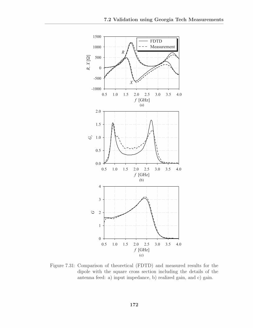
7.2 Validation using Georgia Tech Measurements
0.5 1.0 1.5 2.0 2.5 3.0 3.5 4.0
-1000
-500
0
500
1000
1500
0.5 1.0 1.5 2.0 2.5 3.0 3.5 4.0
0.0
0.5
1.0
1.5
2.0
0.5 1.0 1.5 2.0 2.5 3.0 3.5 4.0
0
1
2
3
4
R,X
[]
f [GHz]
f [GHz]
f [GHz]
Gr
G
(a)
(b)
(c)
FDTD
Measurement
R
X
Figure 7.31: Comparison of theoretical (FDTD) and measured results for thedipole with the square cross section including the details of theantenna feed: a) input impedance, b) realized gain, and c) gain.
172
7.2 Validation using Georgia Tech Measurements
that mark the current contour C. Notice the shift of the contour away from the drive-point gap in order to determine the conduction current. The numerical results for the
input impedance, the realized gain, and the gain are compared with the measured
results in Fig. 7.32. Again, the numerical results are in reasonable agreement with
the measurements.
Notice that for both models the results for the gain is in good agreement with
the measurements. This is because the mismatch between the antenna and the trans-
mission line is not included in this form of the gain. However, the realized gain that
by definition includes the mismatch, is seen to differ for both feed models and to de-
viate from the measured results for frequencies greater than the resonant frequency,
fres ≈ 0.9GHz due to the differences in the reflection coefficient/input impedance.
173

7.2 Validation using Georgia Tech Measurements
0.5 1.0 1.5 2.0 2.5 3.0 3.5 4.0
-1000
-500
0
500
1000
1500
0.5 1.0 1.5 2.0 2.5 3.0 3.5 4.0
0.0
0.5
1.0
1.5
2.0
0.5 1.0 1.5 2.0 2.5 3.0 3.5 4.0
0
1
2
3
4
R,X
[]
f [GHz]
f [GHz]
Gr
G
(b)
(c)
FDTD
Measurement
R
X
f [GHz](a)
Figure 7.32: Comparison of theoretical (FDTD) and measured results for thedipole with the straight cross section omitting the details of theantenna feed: a) input impedance, b) realized gain, and c) gain.
174

CHAPTER 8
Conclusions
The two-arm, conical spiral antenna in free space was shown to have many beneficial
and desirable characteristics over a wide range of frequencies, such as uniform input
impedance, unidirectional radiation and circular polarization. The numerical results
obtained using the FDTD method were validated using accurate measurements per-
formed at Georgia Tech.
A parametric study was performed with the FDTD analysis, and the results from
the study were used to produce new design graphs for this antenna. One graph gives
the useful bandwidth of operation for the antenna, i.e., the bandwidth over which
simultaneously the VSWR is less than 1.5 and the directivity is within −3 dB of itsmaximum value. Other graphs give the parameters that describe the performance of
the antenna (impedance, directivity, half-power beamwidth, front-to-back ratio, and
axial ratio) averaged over this bandwidth. These graphs supplement and extend the
empirical results presented in Dyson’s seminal paper. In general, the results from this
study agree with Dyson’s; a notable difference, however, is that the results from this
study predict a larger useful bandwidth.
Two resistive terminations intended to improve the low-frequency performance
of the CSA were examined: a pair of lumped resistors connected between the arms at
the open end and a thin disc of resistive material connected to the arms at the open
end. The latter is a new configuration that was analyzed to determine the resistance
using conformal mappings. Both terminations were shown to improve the impedance
175

Conclusions
match, front-to-back ratio, and axial ratio of the CSA at low frequencies but to
have a negligible effect on the realized gain. Compared to the lumped resistors, the
resistive sheet was seen to have less conduction loss and slightly better performance
characteristics in some features of the pattern.
The two-arm CSA was investigated when placed directly over the ground with
its axis normal to the surface of the ground. Both qualitative arguments and a
complete FDTD analysis were used to examine how the well-known properties of the
CSA in free space are modified when the antenna is placed over the ground. When
the virtual apex of the antenna is on the air/ground interface, the input impedance
of the antenna was shown to be approximately resistive and nearly constant over
the operational bandwidth of the antenna. The electric field within the ground was
shown to scale with position and frequency, as one would expect from the active-region
concept for the CSA. Also, the electric field in the ground directly below the CSA
was shown to be predominantly circularly polarized. Calculations for a monostatic
GPR that uses a CSA showed how the broadband properties of the CSA could be
used to detect buried objects that scatter an electric field with a component that is
copolarized to the circularly polarized electric field transmitted by the CSA.
The FDTD method was shown to be a powerful tool to analyze and design CSAs
in free space over the ground. The numerical analysis was validated in many ways.
Results for the impedance and the radiated electric field for the unloaded CSA and
the loaded CSA (terminated with lumped resistors) agree well with results published
in the literature. The implementation of the conductive medium was validated with
published analytical and experimental input impedance results for horizontal dipole
antennas placed directly above ground or in tap water. With measurements performed
at Georgia Tech, the FDTD input impedance and realized gain were validated for the
unloaded CSA and the loaded CSAs (terminated using lumped resistors and the
resistive sheet).
Two common FDTD antenna feed models were analyzed for convergence using
the linear dipole antenna with square cross section. It was found that elements of
176

Conclusions
the antenna feed must be properly scaled and positioned for convergence; these are
the physical length of the gap, the size and position of the current contour, as well
as the reference planes within the transmission line. This analysis showed that the
discretization must be chosen finer that one expects in order to reach convergence.
177

APPENDIX A
Analysis of the Resistive Sheet
Termination
The objective of this analysis is to determine the DC resistance between the two
electrodes of angular width δ on the circular disc of diameter D with resistance
per square Rs, see Fig. 4.2b. This is equivalent to solving the electromagnetostatic
problem described in Fig. A.1a: Laplace’s equation must be solved for the potential,
Φ, on the circular disc subject to the boundary conditions Φ = V on one electrode,
Φ = 0 on the other electrode (Dirichlet’s boundary condition) and ∂Φ/∂φ = 0 on
the remainder of the boundary (Niemann’s boundary condition). The solution of this
mixed-boundary problem is accomplished by means of conformal mappings that are
based on analytic functions [52]. Such transformations from one plane to another
preserve the magnitude and sense of angles, and the real and imaginary parts of such
mappings automatically satisfy the two-dimensional Laplace equation. The purpose of
this analysis is to transform the original mixed-boundary problem to a straightforward
geometry with known potential/known DC resistance between the two electrodes.
Thus, two conformal mappings will be used to transform the circular electrodes to a
pair of parallel electrodes with equal DC resistance.
The end points of the circular electrodes, Pmi with i = 1, . . . , 4, can be expressed
mathematically as a function of the diameter of the disc D and the angular width
of the electrodes δ, e.g., Pm1 = (D/2) exp(j(π/2 − δ/2)). Notice that the enclosed
178

Analysis of the Resistive Sheet Termination
= V
= 0
k
l
= 0P1
m
P4
mP3
m
P2
m
m
P1
wP2
wP3
wP4
w
u
vw
-u1 u2-u2 u1
P1
z
P2
zP3
z
P4
z
x
yz
lz
hz
(a)
(b)
(c)
Figure A.1: Drawing detailing the conformal mappings.
179

Analysis of the Resistive Sheet Termination
resistive material lies to the left when the end points are traversed in counterclock
direction (going from Pm1 to Pm
4 ).
The first mapping is a bilinear transformation that transforms the circular disc
in the complex plane m = k + jl into the upper half space in the complex plane
w = u+ jv:
w(m) = j
(2m/D + 1
1− 2m/D
). (A.1)
The result of this transformation is shown in Fig. A.1b. Notice that the electrodes
are now a pair of symmetric strips on the real axis with the end points given by
u2 =1
u1=
cos(δ/2)
1 + sin(δ/2). (A.2)
The resistive material is now located on the positive imaginary half plane and is still
on the left when the points are traversed in the same order as before (going from Pw1
to Pw4 ).
The second mapping is based on the Schwarz-Christoffel transformation, which
transforms a line of constant v into the polygon with N corner points in the z = x+jy
plane. This mapping is illustrated for N = 4 in Fig. A.2 for the general case (left)
and for the special case considered here (right). The general expression for this
transformation can be written as
z = A∫ w
−∞(w′ − w1)
β1π−1(w′ − w2)
β2π−1 . . . (w′ − wN)
βNπ
−1dw′ +B, (A.3)
where the points wi are points along the infinite line with constant v in the w = u+jv
plane that become the corners of the polygon in the z plane. The angle βi is measured
counterclockwise between adjacent segments at the ith corner of the polygon in the
z plane (traversing the polygon from corner 1 to N). In the special case considered
here, the upper half space in the w = u+ jv plane is transformed into the rectangular
region in the z = x+ jy plane with the transformation
z(w) =∫ w
−∞dw′√
w′2 − u22√w′2 − 1/u22
= u2
∫ w/u2
−∞dξ√
(1− ξ2)(1− u42 ξ2). (A.4)
180

Analysis of the Resistive Sheet Termination
w1
-u1
v v
u u
w2
-u2
w3
u2
w4
u1
x x
y y
1
3
2
4
3
2
4
1
Schwarz-Christoffel Transformation (General Case)
Schwarz-Christoffel Transformation (Special Case)
General Case ( = 4):N Special Case:
2 2 2 2
1 2
wdw
w u w u
z
31 2 41 1 1 1
1 2 3 4( ) ( ) ( ) ( )
w
A w w w w w w w w dwz B
1
1
2
23 3
4
4
Figure A.2: Drawing detailing the Schwarz-Christoffel transformation.
The result of this transformation is shown in Fig. A.1c. Notice that the electrodes
are now a pair of parallel strips of width hz separated by the distance lz, and that the
resistive material is again enclosed to the left when the points along the boundary
are traversed from P z1 to P z
4 . Both hz and lz can be written as the distance between
two points, P zi . After using (A.4), we have
lz = |P z3 − P z
2 | = |z(u2)− z(−u2)| = 2u2∫ 1
0
dξ√(1− ξ2)(1− u42 ξ
2)(A.5)
181

Analysis of the Resistive Sheet Termination
= 2u2K(k = u22), (A.6)
and
hz = |P z4 − P z
3 | = |z(u1)− z(u2)| = u2
∫ 1
0
dξ√(1− ξ2)[1− (1− u42) ξ
2](A.7)
= u2K(k =
√1− u42
), (A.8)
where K is the complete elliptic integral of the first kind and modulus k [53]. The
resistance of the disc is now simply determined from the geometry in Fig. A.1c:
R =lzhz
Rs =2K(k = u22)
K(k =
√1− u42
) Rs. (A.9)
with u2 given by (A.2). The normalized resistance, R/Rs, is shown in Fig. A.3 as a
function of the angular width of the electrodes δ. Notice that for δ = 90, the DC
resistance of the sheet reduces to R = Rs.
RR
/s
0 45 90 135 180
0
1
2
3
Figure A.3: Normalized DC sheet resistance as a function of the angular elec-trode width δ.
182
APPENDIX B
Convergence Study for FDTD Feed
Models for Antennas
The properties of antennas, such as the input impedance and the field pattern, are
now routinely determined using numerical techniques for solving Maxwell’s equa-
tions, such as the finite-difference time-domain (FDTD) method. A critical region in
these simulations, particularly for determining the input impedance/admittance, is
the drive point. Often the geometry of the feed point for the actual antenna is quite
complex, so a simplified geometry for the feed point is used in the numerical model.
Differences then exist between the calculated and measured impedances, so a com-
parison of the calculated impedances with the measurements cannot strictly be used
to establish the accuracy of the simulation. In particular, such comparisons cannot
be used to determine if the numerical calculation has converged, which in the case of
the FDTD method generally means that the size of the Yee cell is sufficiently small.
In the following, the convergence of FDTD calculations of the input admittance of a
simple dipole antenna are examined for two different feed models.
Two feed models commonly used for analyzing and designing antennas with the
FDTD method are studied in this work and referred to as the “hard source” and
the “simple feed.” Common properties of both antenna feed models are illustrated
in Fig. B.1. Near the feed region, the antenna is a metallic (PEC) structure which
is separated at the drive-point by a gap of width lg. Outside the feed region, the
183
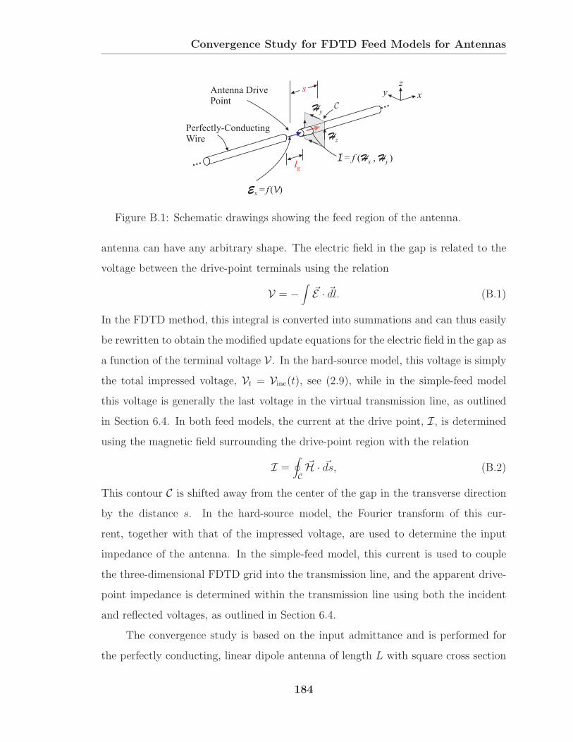
Convergence Study for FDTD Feed Models for Antennas
Antenna DrivePoint
Perfectly-ConductingWire
…
xyz
Hy
Hz
Ex = f ( )V
I = ( , )f H Hx y
s
lg…
Figure B.1: Schematic drawings showing the feed region of the antenna.
antenna can have any arbitrary shape. The electric field in the gap is related to the
voltage between the drive-point terminals using the relation
V = −∫
&E · &dl. (B.1)
In the FDTD method, this integral is converted into summations and can thus easily
be rewritten to obtain the modified update equations for the electric field in the gap as
a function of the terminal voltage V . In the hard-source model, this voltage is simplythe total impressed voltage, Vt = Vinc(t), see (2.9), while in the simple-feed modelthis voltage is generally the last voltage in the virtual transmission line, as outlined
in Section 6.4. In both feed models, the current at the drive point, I, is determinedusing the magnetic field surrounding the drive-point region with the relation
I =∮C&H · &ds, (B.2)
This contour C is shifted away from the center of the gap in the transverse direction
by the distance s. In the hard-source model, the Fourier transform of this cur-
rent, together with that of the impressed voltage, are used to determine the input
impedance of the antenna. In the simple-feed model, this current is used to couple
the three-dimensional FDTD grid into the transmission line, and the apparent drive-
point impedance is determined within the transmission line using both the incident
and reflected voltages, as outlined in Section 6.4.
The convergence study is based on the input admittance and is performed for
the perfectly conducting, linear dipole antenna of length L with square cross section
184
Convergence Study for FDTD Feed Models for Antennas
of equal height and width, w, as shown in Fig. B.2a. This structure is very easy to
discretize with the FDTD method using cubic Yee cells. Here, approximations that
are often introduced in the FDTD analysis of antennas that can affect the convergence
are avoided, such as an approximate equivalence for a round wire, and staircasing of
the geometry for the conductors. For simplicity, at each step in the convergence
study, the next finer discretization is achieved by decreasing the size of the cells by
a factor of two in each direction, i.e., doubling the number of cells along the antenna
in each direction. In the convergence study, the dipole’s length to width ratio is held
fixed at L/w = 30.5 with L = 21.2 cm. Figure B.2b shows the coarsest discretization
used for the antenna: 61 cells along its total length, 2 cells along its width, and 1 cell
across the gap. The shaded areas in this picture are the faces of the FDTD cells along
which the tangential electric field components are set to zero, so they delineate the
boundaries of the perfectly conducting structure. The excitation at the drive point
for the hard-source model (Vt) and within the transmission line (Vinc) for the simplefeed is a differentiated Gaussian voltage pulse, (2.9), with a ratio of characteristic
times between the pulse (τp) and the antenna (τL = L/c) of τp/τL = 1/π ≈ 0.32.
Generally, four different discretizations are studied for convergence of the ad-
mittance results: coarse, medium, fine, and superfine; however, in many results, just
the first three discretizations are shown for clarity. The number of cells per antenna
length, L/∆x, and the number of cells per width, w/∆x, are listed for each discretiza-
tion in Table B.1. In numerical analyses, the number of cells per wavelength at the
highest frequency is of great interest and is often used as an indicator for the accuracy
of the results. A rule of thumb for the FDTD analysis is that at least 10 cells per
shortest wavelength should be used in the simulation to obtain acceptable results, i.e.,
to reduce dispersion to a reasonable level. As shown in Table B.1, even the coars-
est discretization should give negligible dispersion with approximately 30 cells per
shortest wavelength, λmin. In this work, the maximum frequency (minimum wave-
length) is defined to be fmax ≈ 3.5fpeak = 3.5/(2πτp) (λmin = c/fmax ≈ 1.80 τp/τL L),
which is the frequency at which the spectrum decayed to 180to that of the peak
185

Convergence Study for FDTD Feed Models for Antennas
Hy
Hz
Exw
L
Drive Point
xy
z
Schematic Model:
w
FDTD Model:
Faces of CubicFDTD Cells
(a)
(b)
Figure B.2: a) Model of the linear dipole with square cross section, b) discretiza-tion of the model (L/w = 30.5).
value at f = fpeak. A straightforward analysis shows that dispersion is negligible in
this convergence study. Recall, numerical dispersion describes the deviation of the
phase velocity of the numerical wave in the FDTD grid from the speed of light [30].
This effect strongly depends on the propagation direction in the grid and the grid
discretization. Since the pulse propagates in just the x direction (along the metal
rods) in the present case, the simplified numerical dispersion relation for the FDTD
algorithm can be written as
1
c∆tsin
(ω∆t
2
)=
1
∆xsin
(kx∆x
2
), (B.3)
where kx is the numerical wavevector and is related to the numerical phase velocity,
vp, by kx = ω/vp. The dispersion relation, (B.3), can then be solved for the ratio of
186

Convergence Study for FDTD Feed Models for Antennas
Table B.1: Parameters of the discretized linear dipole antenna of square cross section.
coarse medium fine superfine
L/∆ x 61 122 244 488
w/∆x 2 4 8 16
λmin/∆x 35 70 139 279
numerical phase velocity to the speed of light, i.e.,
vp
c=
π
Nλ sin−1 [ 1
CFLsin
(π CFLNλ
)] . (B.4)
Note that this equation contains only normalized parameters such as the number of
cells per wavelength, Nλ = λ/∆x, or the Courant-Friedrichs-Levy (CFL) number,1
CFL = c∆t/∆x, that links the spatial time increment to the dimensions of the Yee
cell. In three-dimensional, cubic FDTD grids, this number is commonly CFL = 0.5.
The results for this ratio vp/c are listed in Table B.2 for various numbers of cells per
shortest wavelength; most of these numbers correspond to the discretizations studied,
see Table B.1. Recall that λ/∆x ≈ 10 is commonly used as a minimum requirement
in FDTD analyses to obtain accurate results at that frequency/wavelength. These
results show that the dispersion will be insignificant for the cases considered.
In the following, the motivation for this work is addressed by presenting the
results for the admittance when the simplest feeding technique is employed for each
discretization. The feeding technique for this “worst case” for convergence is illus-
1The Courant-Friedrichs-Levy condition in a three-dimensional FDTD grid
c∆t
√1∆x2
+1∆y2
+1∆z2
≤ 1
must be satisfied for stability for the finite-difference scheme of second order in time and space.
When cubic cells are chosen, this condition simplifies to
c∆t
∆x= CFL ≤ 1√
3.
187

Convergence Study for FDTD Feed Models for Antennas
Table B.2: Ratio of numerical phase velocity to the speed of light for differentdiscretizations.
λmin/∆x 10 35 70 139 279(coarse) (medium) (fine) (superfine)
vp/c 0.98726 0.99899 0.99975 0.99994 0.99998
trated in Fig. B.3 for the first three discretizations (coarse, medium, and fine). The
left side is the “bird’s eye” view of the feed region, the center shows the top view
of the feed, and the right side shows the cross-sectional view of the drive point. In
each discretization, a one-cell gap is employed for each discretization, i.e., the phys-
ical length of the gap differs for each discretization, see the center of Fig. B.3, while
the total length of the antenna remains the same. Here, just a single electric field in
the center of the gap is updated with the modified update equation, based on (B.1).
The current is determined by integrating directly around the drive-point gap, i.e., the
contour is not shifted in the transverse direction and has the smallest cross-sectional
area to just enclose the surface of the conductor. The magnetic fields, Hy and Hz,
that mark the rectangular contour C are seen to move closer to the antenna conduc-tor the finer the discretization. The distance between the surface of the conductor
and the magnetic field component is exactly a half spatial step of the corresponding
grid. The results for this convergence study are shown in Fig. B.4 for the first three
discretizations. Figure B.4a is for the hard-source model and Fig. B.4b is for the
simple feed. Obviously, the results for either feed are not converging with increasing
discretization. Recall that these feed elements are chosen in the simplest and usually
most common way for each discretization; thus, some of these choices can be expected
to cause the results not to converge.
In the remainder of this section, it will be shown that it is crucial to properly po-
sition and scale the elements in the feed model for convergence. Figure B.5 illustrates
that different geometrical lengths of the gap introduce a change in the susceptance.
As shown schematically, the decrease in length increases the capacitive effect at the
188

Convergence Study for FDTD Feed Models for Antennas
xyz
xy
z
y
Hy
Ex
Ex
Hy
Hz
Hz
Coarse:
Medium:
Fine:
C
Figure B.3: Feeding techniques shown for the first three discretizations (worstcase for convergence).
drive point. To avoid this source of error, the length of the drive point-gap must be
the same for each discretization. Another important effect must be considered in this
study: the fringing of the electric field in the vicinity of the gap, shown schemati-
cally in Fig. B.6. Fringing occurs since charges accumulate at the terminals of the
antenna conductors that represent a discontinuity in the antenna geometry. Obvi-
ously, by varying the radial extent of the contour when placed in the vicinity of the
gap, different portions of the fringing field are included in the current contour. The
contour surrounding the gap thus yields a displacement current; however, since the
calculation of the input impedance for the hard-source model and the components of
the transmission line require the total current into the antenna terminals, an offset
contour with s > lg/2 should be chosen instead to yield the conduction current.
The above criteria are met in the following feeding technique, referred to as “best
case” for convergence. Schematic drawings of the feed region are shown in Fig. B.7.
189

Convergence Study for FDTD Feed Models for Antennas
GB
,[m
S]
0.0 0.5 1.0 1.5 2.0 2.5
-4
0
4
8
12
16
f [GHz]
G
B
GB
,[m
S]
0.0 0.5 1.0 1.5 2.0 2.5
-4
0
4
8
12
16
f [GHz]
G
B
CoarseMediumFine
(a)
(b)
Figure B.4: Results for the input admittance in the worst case for convergence:a) hard-source model and b) simple feed.
Ccoarse Cmedium Cfine< <
Figure B.5: Schematic illustration of the change of the susceptance with varyinglength of the gap.
Here, the drive-point gap properly scales for each discretization by keeping the length
of the gap constant with lg = w/2. For discretizations finer than the coarsest one, this
requires multiple-cell gaps. In order to apply the voltage in the gap more uniformly, all
190
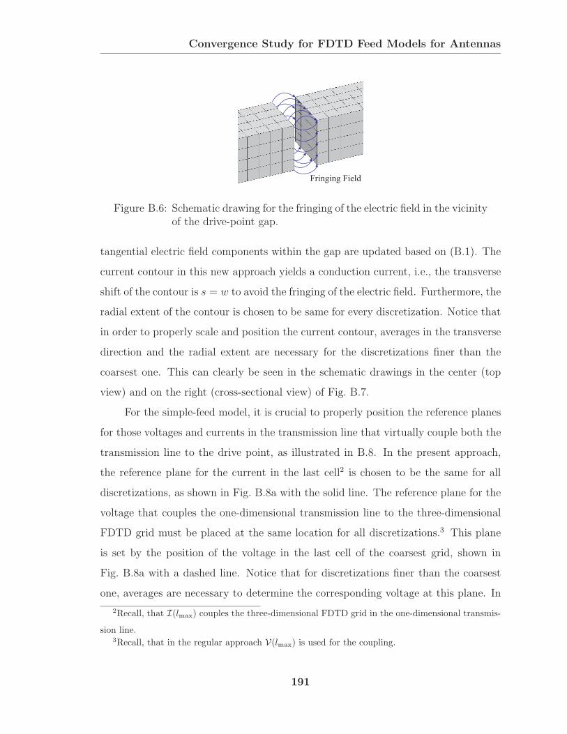
Convergence Study for FDTD Feed Models for Antennas
Fringing Field
Figure B.6: Schematic drawing for the fringing of the electric field in the vicinityof the drive-point gap.
tangential electric field components within the gap are updated based on (B.1). The
current contour in this new approach yields a conduction current, i.e., the transverse
shift of the contour is s = w to avoid the fringing of the electric field. Furthermore, the
radial extent of the contour is chosen to be same for every discretization. Notice that
in order to properly scale and position the current contour, averages in the transverse
direction and the radial extent are necessary for the discretizations finer than the
coarsest one. This can clearly be seen in the schematic drawings in the center (top
view) and on the right (cross-sectional view) of Fig. B.7.
For the simple-feed model, it is crucial to properly position the reference planes
for those voltages and currents in the transmission line that virtually couple both the
transmission line to the drive point, as illustrated in B.8. In the present approach,
the reference plane for the current in the last cell2 is chosen to be the same for all
discretizations, as shown in Fig. B.8a with the solid line. The reference plane for the
voltage that couples the one-dimensional transmission line to the three-dimensional
FDTD grid must be placed at the same location for all discretizations.3 This plane
is set by the position of the voltage in the last cell of the coarsest grid, shown in
Fig. B.8a with a dashed line. Notice that for discretizations finer than the coarsest
one, averages are necessary to determine the corresponding voltage at this plane. In
2Recall, that I(lmax) couples the three-dimensional FDTD grid in the one-dimensional transmis-
sion line.3Recall, that in the regular approach V(lmax) is used for the coupling.
191
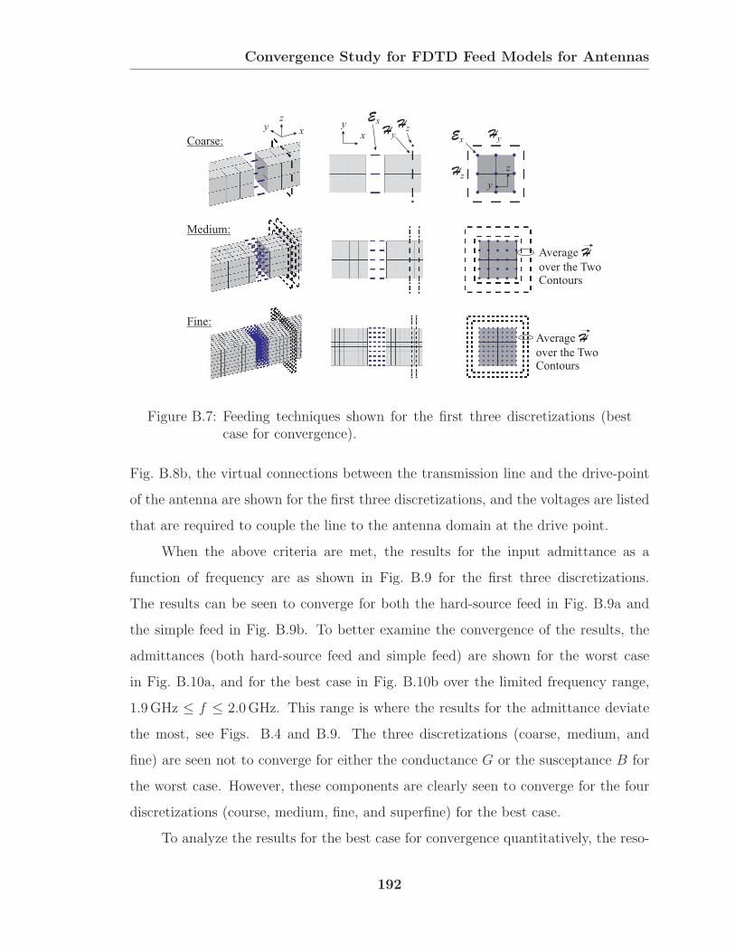
Convergence Study for FDTD Feed Models for Antennas
xyz
xy
z
y
Hy
Ex
ExHy
Hz
Hz
Coarse:
Medium:
Fine:
Average
over the TwoContours
H
Average
over the TwoContours
H
Figure B.7: Feeding techniques shown for the first three discretizations (bestcase for convergence).
Fig. B.8b, the virtual connections between the transmission line and the drive-point
of the antenna are shown for the first three discretizations, and the voltages are listed
that are required to couple the line to the antenna domain at the drive point.
When the above criteria are met, the results for the input admittance as a
function of frequency are as shown in Fig. B.9 for the first three discretizations.
The results can be seen to converge for both the hard-source feed in Fig. B.9a and
the simple feed in Fig. B.9b. To better examine the convergence of the results, the
admittances (both hard-source feed and simple feed) are shown for the worst case
in Fig. B.10a, and for the best case in Fig. B.10b over the limited frequency range,
1.9GHz ≤ f ≤ 2.0GHz. This range is where the results for the admittance deviate
the most, see Figs. B.4 and B.9. The three discretizations (coarse, medium, and
fine) are seen not to converge for either the conductance G or the susceptance B for
the worst case. However, these components are clearly seen to converge for the four
discretizations (course, medium, fine, and superfine) for the best case.
To analyze the results for the best case for convergence quantitatively, the reso-
192

Convergence Study for FDTD Feed Models for Antennas
…
…
…
…
…
…
xyz
Hy
Hy
Hy
Hz
Hz
Hz
Vn+1
( )lmaxE x
n+1
dp
E x
n+1
dp
E x
n+1
dp
Vn+1
( )+lmax Vn+1
( -1)lmax
Vn+1
( -1)+lmax Vn+1
( -2)lmax
Coarse:
Medium:
Fine:
Coarse Medium Fine1D Line:
(a)
(b)
Plane for I (3D 1D)
Plane for V (3D 1D)
Figure B.8: a) Proper scaling of the reference planes in the transmission line,b) correct virtual connection of the transmission line at the feedpoint.
nant frequency and the conductance at anti-resonance (the point where B is zero for
the second time, λres ≈ L or equivalently fres = c/L) are determined for the hard-
source feed, see Fig. B.9. The results for this analysis are listed in Table B.3. Clearly,
the two parameters fres and Gres are seen to converge with increasing discretization;
the deviation in the resonant frequency between the coarsest and the finest grid is
approximately 2% and the deviation in the conductance is 4%. It should be noted
that for errors in these parameters less than about 2% the number of cells at that
193

Convergence Study for FDTD Feed Models for Antennas
GB
,[m
S]
f [GHz]
GB
,[m
S]
f [GHz](a)
(b)
0.0 0.5 1.0 1.5 2.0 2.5
-4
0
4
8
12
16
0.0 0.5 1.0 1.5 2.0 2.5
-4
0
4
8
12
16
CoarseMediumFine
Figure B.9: Results for the input admittance in the best case for convergence:a) hard-source model and b) simple feed.
particular wavelength, λ must be at least λ/∆x ≈ 100.
In conclusion, for the FDTD feed models studied (hard source and simple feed)
to converge the elements of the feed must be properly scaled and positioned. These
elements are the length of the drive-point gap and the size and position of the cur-
rent contour C. For the simple feed, this also includes the proper positioning of thereference plane for the voltage in the transmission line that couples the line into the
drive point of the antenna. It was found that the discretization for convergence has
to be much finer than one typically expects based on the negligible dispersion alone.
194
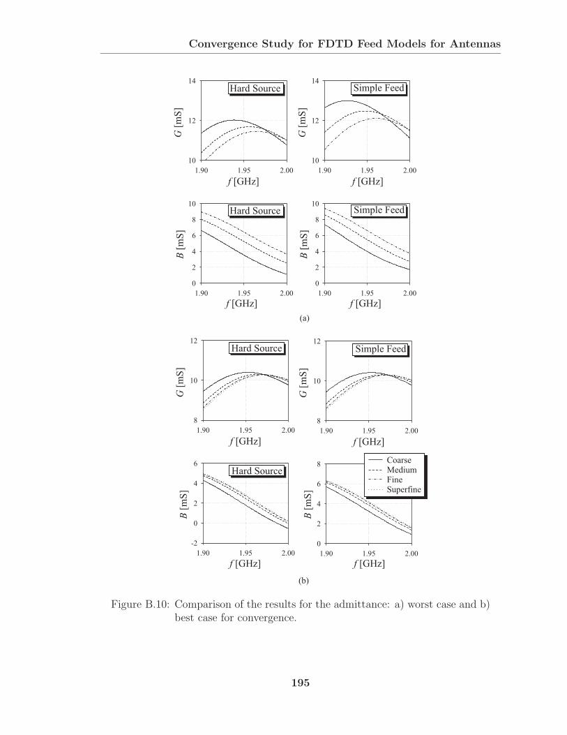
Convergence Study for FDTD Feed Models for Antennas
1.90 1.95 2.00
10
12
14
1.90 1.95 2.00
10
12
14
1.90 1.95 2.00
8
10
12
1.90 1.95 2.00
8
10
12
G[m
S]
f [GHz]
1.90 1.95 2.00
0
2
4
6
8
10
B[m
S]
f [GHz]1.90 1.95 2.00
0
2
4
6
8
10
B[m
S]
f [GHz]
1.90 1.95 2.00
-2
0
2
4
6
B[m
S]
f [GHz]1.90 1.95 2.00
0
2
4
6
8
B[m
S]
f [GHz]
G[m
S]
f [GHz]G
[mS
]
f [GHz]
G[m
S]
f [GHz]
Hard Source
Hard Source
Simple Feed
Simple Feed
Hard Source
Hard Source
Simple Feed
(a)
(b)
CoarseMediumFineSuperfine
Figure B.10: Comparison of the results for the admittance: a) worst case and b)best case for convergence.
195

Convergence Study for FDTD Feed Models for Antennas
Table B.3: Resonant frequencies and the conductances at anti-resonance forthe hard source (best case for convergence).
coarse medium fine superfine
fres [GHz] 1.17 1.18 1.19 1.19
Gres [mS] 1.91 1.86 1.83 1.83
λres/∆x 74 146 291 581
196
Bibliography
[1] A.W. Love, “Antennas for Satellites,” IEEE Potentials, vol. 6, pp. 22–25, 1987.
[2] M. Kanda, “EMC Strategies: Industrial and Reseach Perspectives,” Interna-tional Conference on Electromagn. Interference and Compat., pp. 403–404, Dec.1995.
[3] S. Tonfani, A. Ondrejka, M. Kanda, “A Time-Domain Method for Characterizingthe Reflection Coefficient of Absorbing Materials from 30 to 1000 MHz,” IEEETrans. Electromagn. Compat., vol. 33, pp. 234–240, 1991.
[4] G. Arjavalingam, Y. Pastol, J.M. Halbout, W.M. Robertson,“Optoelectronically-Pulsed Antennas: Characterization and Applications,”IEEE Antennas Propagat. Mag., vol. 33, pp. 7–11, 1991.
[5] T. Iwasaki, A. Freundorfer, K. Iizuka, “A Unidirectional Semi-Circle SpiralAntenna for Subsurface Radars,” IEEE Trans. Electromagn. Compat., vol. 36,pp. 1–6, 1994.
[6] V.H. Rumsey, “Frequency Independent Antennas,” IRE Intern. Conv. Record,pp. 114–118, 1957.
[7] V.H. Rumsey, Frequency Independent Antennas, Academic Press, New York,NY, 1966.
[8] J.D. Dyson, “The Equiangular Spiral Antenna,” IRE Trans. Antennas Propagat.,vol. AP-7, pp. 181–187, 1959.
[9] J.D. Dyson, “The Unidirectional Equiangular Spiral Antenna,” IRE Trans.Antennas Propagat., vol. AP-7, pp. 329–334, 1959.
[10] J.D. Dyson, P.E. Mayes, “New Circularly Polarized Frequency-Independent An-tennas with Conical Beam or Omnidirectional Patterns,” IRE Trans. AntennasPropagat., vol. AP-9, pp. 334–342, July 1961.
[11] E.C. Jordan, G.A. Deschamps, J.D. Dyson, R.E. Mayes, “Development in Broad-band Antennas,” IEEE Spectrum, vol. 1, pp. 58–71, April 1964.
197

BIBLIOGRAPHY
[12] J.D. Dyson, “The Characteristics and Design of the Conical Log-Spiral An-tenna,” IEEE Trans. Antennas Propagat., vol. AP-13, pp. 488–499, 1965.
[13] Y.S. Yeh, K.K. Mei, “Theory of Conical Equiangular-Spiral Antennas Part I –Numerical Technique,” IEEE Trans. Antennas Propagat., vol. AP-15, pp. 634–639, 1967.
[14] Y.S. Yeh, K.K. Mei, “Theory of Conical Equiangular-Spiral Antennas Part II –Current Distributions and Input Impedances,” IEEE Trans. Antennas Propagat.,vol. AP-16, pp. 14–21, 1968.
[15] E.K. Miller, J.A. Landt, “Short-Pulse Characteristics of the Conical Spiral An-tenna,” IEEE Trans. Antennas Propagat., vol. AP-25, no. 5, pp. 621–626, 1977.
[16] R.G. Wills, “A Submarine Multifunction Antenna,” Communication & Broad-casting, vol. 9, no. 3, pp. 39–45, 1985.
[17] P.A. Ramsdale, P.W. Crampton, “Properties of 2-arm Conical Equiangular Spi-ral Antenna over Extended Bandwidth,” IEE Proc. H, vol. 128, pp. 311–316,1981.
[18] R. Mittra, K.E. Jones, “How to Use k − β Diagrams in Log-Periodic AntennaDesign,” Microwaves, pp. 18–26, June 1965.
[19] J.D. Krauss, Antennas, Chap. 7, Mc Graw-Hill, 1988.
[20] IEEE Standard Definition of Terms for Radio Wave Propagation, Institute ofElectrical and Electronics Engineers, Inc., 1993.
[21] G.S. Smith, An Introduction to Classical Electromagnetic Radiation, CambridgeUniversity Press, Cambridge, UK, 1997.
[22] Antenna Standards Committee of the IEEE Antennas and Propagation Society,IEEE Standard Definition of Terms for Antennas, Institute of Electrical andElectronics Engineers, Inc., 1993.
[23] R.W.P. King, G.S. Smith, Antennas in Matter: Fundamentals, Theory, andApplications, Chap. 12, MIT Press, Cambridge, MA, 1981.
[24] R. Apfeldorfer, “A Study of Wave Propagation in Lossy Media,” GRA Report,School of ECE, Georgia Tech, 1998.
[25] T.P. Montoya, Vee Dipole Antennas for use in Short-Pulse Ground-PenetratingRadars, Ph.D. thesis, Georgia Institute of Technology, Atlanta, GA, 1998.
[26] W.C. Chew, Waves and Fields in Inhomogeneous Media, IEEE Press, NY, 1995.
198

BIBLIOGRAPHY
[27] S. Vitebskiy, L. Carin, M.A. Ressler, F.H. Le, “Ultra-Wideband, Short-PulseGround-Penetrating Radar: Simulation and Measurement,” IEEE Trans. Geo-science and Remote Sensing, vol. 35, pp. 762–772, 1997.
[28] K.S. Yee, “Numerical Solution of Initial Boundary Value Problems InvolvingMaxwell’s Equations in Isotropic Media,” IEEE Trans. Antennas Propagat., vol.AP-14, pp. 302–307, 1966.
[29] K.L. Shlager, J.B. Schneider, “A Selective Survey of the Finite-Difference Time-Domain Literature,” IEEE Antennas and Propagation Magazine, vol. 37, pp.39–57, 1995.
[30] A. Taflove, Computational Electrodynamics: The Finite-Difference Time-Domain Method, Artech House, Norwood, MA, 2000.
[31] A. Taflove, Advances in Computational Electrodynamics: The Finite-DifferenceTime-Domain Method, Artech House, Norwood, MA, 1998.
[32] G.E. Moore, “Cramming More Components Onto Integrated Circuits,” Elec-tronics, vol. 38, pp. 114–117, 1965.
[33] K.L. Shlager, G.S. Smith, J.G. Maloney, “Accurate Analysis of TEM HornAntennas for Pulse Radiation,” IEEE Trans. Electromagn. Compat., pp. 414–423, 1996.
[34] J.G. Maloney, G.S. Smith, “Modeling of Antennas,” in Advances in Computa-tional Electrodynamics: The Finite-Difference Time-Domain Method, A. Taflove,Ed. Artech House, Norwood, MA, 1998.
[35] G.S. Smith, M.P. Kesler, J.G. Maloney, “Dipole Antennas used with All-Dielectric, Woodpile Photonic-Bandgap Reflectors: Gain, Field Patterns, andInput Impedance,” Microwave and Optical Technology Letters, pp. 191–196,1999.
[36] J.P. Berenger, “A Perfectly Matched Layer for the Absorption of ElectromagneticWaves,” Journal of Computational Physics, vol. 114, pp. 185–200, 1994.
[37] Z.S. Sacks, D.M. Kingsland, R. Lee, J.F. Lee, “A Perfectly Matched AnisotropicAbsorber for Use as an Absorbing Boundary Condition,” IEEE Trans. AntennasPropagat., vol. 43, pp. 1460–1463, 1995.
[38] S. Gedney, “An Anisotropic Perfectly Matched Layer-Absorbing Medium for theTruncation of FDTD Lattices,” IEEE Trans. Antennas Propagat., vol. 44, pp.1630–1639, 1996.
[39] W.C. Chew, W.H. Weedon, “A 3-D Perfectly Matched Medium from Modi-fied Maxwell’s Equations with Stretched Coordinates,” Microwave and OpticalTechnology Letters, vol. 7, pp. 599–604, 1994.
199

BIBLIOGRAPHY
[40] S.D. Gedney, A. Taflove, “Perfectly Matched Layer Absorbing Boundary Con-ditions,” in Advances in Computational Electrodynamics: The Finite-DifferenceTime-Domain Method, A. Taflove, Ed. Artech House, Norwood, MA, 1998.
[41] T.W. Hertel, “Pulse Radiation from an Insulated Antenna: An Analogue ofCherenkov Radiation from a Moving Charge,” M.S. thesis, Georgia Institute ofTechnology, Atlanta, GA, 1998.
[42] J.G. Maloney, G.S. Smith, “The Efficient Modeling of Thin Material Sheets inthe Finite-Difference Time-Domain (FDTD) Method,” IEEE Trans. AntennasPropagat., vol. 40, pp. 323–330, 1992.
[43] J.G. Maloney, G.S. Smith, “A Comparison of Methods for Modeling ElectricallyThin Dielectric and Conducting Sheets in the Finite-Difference Time-Domain(FDTD) Method,” IEEE Trans. Antennas Propagat., vol. 41, pp. 690–694, 1993.
[44] K.R. Umashankar, A. Taflove, B. Beker, “Calculation and Experimental Vali-dation of Induced Currents on Coupled Wires in an Arbitrary Shaped Cavity,”IEEE Trans. Antennas Propagat., vol. 35, pp. 1248–1257, 1987.
[45] J.G. Maloney, Analysis and Synthesis of Transient Antennas using the Finite-Difference Time-Domain (FDTD) Method, Ph.D. thesis, Georgia Institute ofTechnology, Atlanta, GA, 1992.
[46] P.S. Pacheco, W.C. Ming, MPI Users Guide in Fortran, 1997.
[47] L.E. Vogler, J.L. Noble, “Curves of Ground Proximity Loss for Dipole Antennas(a Digest),” Journal of Research of National Bureau of Standards—D. RadioPropagation, vol. 67D, pp. 567–568, 1963.
[48] L.E. Vogler, J.L. Noble, “Curves of Ground Proximity Loss for Dipole Antennas,”Technical Note 175 , National Bureau of Standards, 1963.
[49] A. Karwowski, K.A. Michalski, “A Comparative Study of Several Techniques forModeling a Horizontal Wire Antenna over a Lossy Half-Space,” Radio Science,vol. 6, pp. 922–928, 1987.
[50] C. A. Balanis, Antenna Theory Analysis and Design, John Wiley & Sons, Inc.,New York, NY, 1997.
[51] Antenna Standards Committee of the IEEE Antennas and Propagation Soci-ety, IEEE Standard Test Procedures for Antennas, Institute of Electrical andElectronics Engineers, Inc., 1979.
[52] M.R. Spiegel, Schaum’s Outline of Theory and Problems of Complex Variableswith an Introduction to Conformal Mapping and its Application, Schaum, NewYork, 1964.
200

BIBLIOGRAPHY
[53] I.S. Gradshteyn, I.M. Ryzhik, Table of Integral, Series, and Products, AcademicPress, San Diego, 1994.
201

VITA
Thorsten W. Hertel was born in Holzminden, Germany, on April 19, 1974. He at-
tended the Campe Gymnasium in Holzminden and graduated from there in 1993.
He received the Vordiplom in Electrical Engineering from the Technische Universitat
Braunschweig, Germany, in 1996. The same year he entered the Graduate Program in
Electrical and Computer Engineering at the Georgia Institute of Technology, Atlanta,
GA (USA), where he was a graduate teaching assistant, and a graduate research as-
sistant. He received the M.S. degree in Electrical and Computer Engineering from
the Georgia Institute of Technology in 1998 with a thesis entitled: “Pulse Radiation
from an Insulated Antenna: An Analogue of Cherenkov Radiation from a Moving
Charge.”
His special interests include numerical modeling with the Finite-Difference Time-
Domain (FDTD) Method and antenna analysis and design.
202


![Design and Fabrication of Antennas Using 3D PrintingThe second design is a spiral antenna. Spiral antennas are circularly polarized wideband antennas [17] with geometries determined](https://img.dokumen.tips/doc/110x75/612a24e510b629476b55dcc8/design-and-fabrication-of-antennas-using-3d-printing-the-second-design-is-a-spiral.jpg)