Critical Infrastructure Resiliency

in the Hampton Roads Area of Virginia

Regional Infrastructure Modeling and Simulation Report Number V08-001

(Milestone Report Task IV)

Prepared for:

City of Hampton, Virginia

Prepared by: Virginia Modeling, Analysis and Simulation Center

Old Dominion University, Norfolk, VA 223529

NOTE: This document was prepared primarily based on publicly available data and information as well as interviews with officials from local jurisdictions, infrastructure service providers and military organizations. Comments and opinions in this draft report have not been reviewed by any of these organizations

ii

Task Objectives:

Task IV was initiated to model relationships between key infrastructure systems in order to reasonably simulate the consequences of specific failure modes from natural or deliberate adverse events. Successful model(s) would serve as the basis for simulation of selected hazard events and the simulated impacts of optional mitigation actions. The Task included five principal elements: Model four infrastructure systems (communications, energy, transportation, and

water) serving the Hampton Roads region Validate models to document accuracy Run models to obtain magnitude of impact on infrastructures from selected

hazard/threat events Develop illustrative event-related scenarios to identify failures and indicate areas

of service loss Provide probabilistic estimates of threat and consequences for the selected

scenarios, where possible

Approach:

Two natural disasters (hurricane and pandemic flu) formed the primary basis for the modeling effort. Input/output relationships were identified between four critical infrastructures chosen for analysis - energy, water/wastewater, transportation and communications - that would be affected by a hurricane of the specified magnitude and a flu pandemic.

The project utilized a number of computer models to support project tasks. Existing available candidate computer models were reviewed and demonstrated, with final selection made by the Project Team with input from the advisory committee(s). Detailed specifications, data requirements, and performance capabilities for all computer models to be used were developed and reviewed by the Project Team and advisory committee(s).

In reviewing and selecting models, the Project Team communicated with cognizant federal, national laboratory, Commonwealth, and military personnel to ensure critical information regarding input disaster parameters and output impact effects realistic and will provide useable information for the jurisdictions.

TABLE OF CONTENTS

Critical Infrastructure Resiliency in the Hampton Roads Area of Virginia................................... i Critical Infrastructure Resiliency Progress Report ......................................................................... 1 1 Introduction............................................................................................................................. 1 2 Critical Infrastructure Overview............................................................................................. 2

2.1 Transportation ................................................................................................................. 2 2.2 Energy ............................................................................................................................. 2 2.3 Communication............................................................................................................... 2 2.4 Potable Water.................................................................................................................. 2 2.5 Waste Water.................................................................................................................... 2

3 Disaster Modeling................................................................................................................... 2 4 Background Research ............................................................................................................. 3

4.1 Critical Infrastructure Functional Decomposition .......................................................... 3 4.2 Critical Infrastructure Relations...................................................................................... 4

5 Modeling and Simulation Approach....................................................................................... 6 5.1 Approach Outline............................................................................................................ 6 5.2 Scenario Preparation Tool............................................................................................... 9

5.2.1 Model Generation ................................................................................................... 9 5.2.2 Generating Execution Scenarios. .......................................................................... 10

5.3 Agent-Based Model Execution Engine......................................................................... 10 5.4 External Infrastructure Simulation................................................................................ 12 5.5 ABM Communication Bus ........................................................................................... 14

5.5.1 Simulation Control................................................................................................ 15 5.5.2 Visualization ......................................................................................................... 15 5.5.3 Data collection ...................................................................................................... 16

1

Critical Infrastructure Resiliency Progress Report

1 Introduction This report outlines the work conducted by Old Dominion University’s Virginia Modeling Analysis and Simulation Center (VMASC) on the modeling and simulation portion of the Critical Infrastructure Resilience for the Hampton Roads Region project. The portion of the work conducted at VMASC is focused on modeling critical infrastructures and demonstrating a simulation framework that assists with identification of potentially dangerous interdependencies that are not apparent by a simple review. The premise of the work is that interdependent infrastructures when stressed by natural disasters will fail in ways that are currently unplanned for, primarily because of unforeseen cascading effects that propagate failures across these infrastructures. Such cascading failures bypass traditional resilience efforts that focus on individual infrastructures and are particularly important to address. The goals of the modeling and simulation framework will allow examination of selected region infrastructure vulnerabilities and interdependencies and support the evaluation of resilience to natural technological and terrorist risk scenarios, examine military and civilian infrastructure interdependencies, and allow decision makers to prioritize investments in regional resilience on the basis of risk cost and benefit trade-offs. Work done as part of this task focused on developing a critical infrastructure interdependency model, along with a prototype that will be used to demonstrate the simulation framework. Part of this effort was put towards examination of a significant amount of GIS data in order to assess the automatic transformation of such data into model inputs. Subsequently, functional decomposition and input/output analysis was used to identify infrastructure clusters and the nature of the relationships. The result of this analysis was an influence diagram that not only provided insight on the extend to which interdependencies could make the overall system vulnerable, but provided a basis for development of a simulation framework that through interactive simulations can exercise and pinpoint such interdependencies. Finally, a prototype tool was designed and is currently under development. The purpose of this tool is to demonstrate the feasibility of the modeling approach. The prototype tool however, is not meant to be a mature or robust product that can be used by decision makers at this point. Many reasons contribute to the current status of the tool. This is cutting edge research and there is a natural period required to reach maturation. Another reason is that despite the volume of existing GIS data, detailed and properly attributed data required for accurate model inputs does not exist or is difficult to obtain. This is because of confidentiality and security concerns as well as largely different methods by which agencies tag the data. The prototype tool uses actual data when possible; however, when adequate data is not available, synthetic data is used. The remainder of this report contains a background section on the critical infrastructures that were analyzed, the sources of data used for the prototype tool and a detailed description of the agent-based modeling and simulation framework.

2

2 Critical Infrastructure Overview The infrastructures selected for further research in this project include ground transportation, energy delivery, wireless communication, potable water delivery and waste water collection & disposable. Each infrastructure consists of numerous individual components and sub-models. For purposes of this project, the scope of interest in each infrastructure was limited to make the overall simulation feasible. At the same time, the level of detail was such that disaster effects could be captured and used in the larger model to identify cascading effects.

2.1 Transportation We focused on ground transportation, specifically accessibility of resident’s to evacuation routes, emergency responder’s to an area in need, and personnel to critical facilities. Failures in the transportation infrastructure can affect the movement of goods, potable water, waste water, energy, communications, and other resources along roads, railways, airways, waterways, transmission lines, pipelines, and communication towers.

2.2 Energy Energy is a critical infrastructure because of its vulnerability to natural as well as man-made disasters. In its basic form, the energy infrastructure is responsible for the acquisition or generation, transmission, distribution, and storage of electricity and includes power plants, transmission lines, substations, distribution lines, distribution poles, and transformers for purposes of satisfying residential, commercial, industrial, and transportation demands.

2.3 Communication The general scope of the communication infrastructure is too complex to effectively analyze and incorporate in a model. In general, the infrastructure includes transmission and reception of data and information via land lines, cell phones, radio, and the Internet using satellites, communication towers, routers, switching stations, junction boxes, phone lines, cable, and fiber optics. For purposes of this project, the scope was limited to cell-phone communications which depend largely on the operation of a wide network of cell-phone towers.

2.4 Potable Water Potable water has both industrial and residential applications. A functioning infrastructure ensures the transportation of potable water from a source to a treatment plant to the end user through a network consisting of wells, reservoirs, pipes, pumps, nodes, valves, fixtures, and storage tanks.

2.5 Waste Water The waste water infrastructure is responsible for the collection, treatment, and disposal of waste water through a network consisting of pipes, pumps, nodes, valves, fixtures, access points (manholes), and treatment plants.

3 Disaster Modeling In order to model the two natural disasters (hurricane and pandemic flu), we identified input/output relationships among infrastructures that would be affected by a hurricane of the specified magnitude and a pandemic flu. In the case of the pandemic flu, the primary factor

3

affecting infrastructure operation is lack of minimum required personnel to operate a facility. In the case of a hurricane, excessive wind and flooding are the primary inputs to the failure models of each infrastructure.

4 Background Research Based on subject matter expert knowledge (from both literature review and interviews with experts specific to the Hampton Roads region) a functional description was developed of the basics for each of the five infrastructure areas. Each infrastructure was broken down into the broad functional areas that are required for that infrastructure to perform its duties. These broad functional descriptions were then subjected to further review and comment by subject matter experts contributing to the overall project.

4.1 Critical Infrastructure Functional Decomposition An example of one such functional description can be seen in Figure 1.

EnergyGeneration

EnergyTransmission

EnergyDemand

Generator Facility

•Type•Location•Capacity

Lines

•Type•Location•Capacity

Substation

•Type•Location•Rating

Transformer

•Type•Location•Capacity

Terminal Node

•Type•Location•Demand

EnergyDistribution

Lines

•Type•Location•Capacity

Substation

•Type•Location•Rating

Transformer

•Type•Location•Capacity

Energy Infrastructure FD

Figure 1 – Example Functional Decomposition.

The four columns each represent a broad function of the Energy delivery infrastructure. The first column represents energy generation. This could be (depending on the particular energy delivery system within a region that is being modeled) a coal or hydro driven power plant, or the city gateway of a pipeline, or even a nuclear generator. In any case, it represents (for the region being modeled) the function of origination of energy within that system. The next two columns represent, respectively, the transmission of energy (in a bulk, or high capacity, form) and then the distribution of energy (from the transmission structure, down to individual consumers). Finally, the fourth column represents the energy demand that a specific energy consumption site would generate – for instance, a neighborhood of residential homes, or a factory, or a hospital. Each of these functional areas was then decomposed, into the elements (which would become the nodes or arcs in a graphical representation of the infrastructure) that enabled that particular area

4

of functionality. For instance, under the Energy Transmission column, we see the three elements of lines, substations, and transformers. The lines could represent high capacity pipelines, or high capacity electrical transmission lines. The substations would be where switching, load balancing, and so on would take place. Finally, transformers would be points where capacity could change (from Transmission to Distribution), and other related activities. In this we, we identify the three broad types of elements that make the energy transmission function of the energy delivery infrastructure work. This level of functional decomposition was performed for each of the five critical infrastructure areas. Consideration for specific examples of those infrastructure types other than those existing in Hampton Roads was made in the project, which potentially broadens the applicability of the research.

4.2 Critical Infrastructure Relations Once the functional decompositionof the various infrastructures was completed, then the application of attributes to the elements within functional areas was the next step. As the elements were intended to be represented by agents in an agent based model, the attributes of those agents would have to come from this conceptual model. And since the overall goal of the project was to highlight the interaction of different layers of the infrastructure types, that was the perspective that the functional area elements were considered when developing these lists of elements. In the Energy example diagram given above, it can be seen that under each element, only a few example attributes are given. In order to complete this next step, further attributes would be needed (from the perspective of infrastructure interoperability). As the model was representing a critical infrastructure that was operational, it was determined that the requirements for attributes would be the input and output for each element that enabled its functionality or that arose from its proper functionality. An example of the I/O analysis that determined the attributes for the Energy functional area elements is shown in Figure 2.

5

Energy Infrastructure I/O

• Energy Generation– Inputs

• People• Policy• Power• Communications• Consumables (fuel, cooling water, etc)• Energy

– Outputs• Energy• Communications• Waste

• Energy Transmission (lines)– Inputs/Outputs

• Energy

• Energy Transmission (transformers)– Inputs/Outputs

• Energy

• Energy Transmission (subsystems)– Inputs

• PPPCC• Energy

– Outputs• Energy• Communications

• Energy Consumption (terminal)– Inputs

• Energy

• Energy Distribution (lines)– Inputs/Outputs

• Energy

• Energy Distribution (transformers)– Inputs/Outputs

• Energy

• Energy Distribution (subsystems)– Inputs

• PPPCC• Energy

– Outputs• Energy• Communications

Figure 2 – Sample Input/Output Relationship.

From this chart, it can bee seen that for the Energy Generation element, that there are a number of inputs and outputs. These include (as inputs) people, policy, power, communications, consumables, and energy. A few notes here might be helpful. When people are considered as an input or output, this represents elements from the surrounding population that enable the operation of the element – the workers, administration, support, etc. Policy as in input requires that the element be capable of getting information from the governing bodies that control it (either the infrastructure “company”, or the government, or emergency services) that might cause it to stop functioning in an emergency, or to direct other activities that affect its normal functioning. Power is representative of power needed for the element to function properly (for instance, a coal fired power plant may have some electricity demand from the outside perhaps to start up, or just for normal functionality of lights, offices, etc). The communications input represents the need for the element to be connected to other elements that need to communicate with it for normal operation (demand, start/stop instructions, safety checks, etc). Consumables represent the requirement to operation machines, people, or other resources that are internally required for the functionality of the element. Finally, in this case, energy as an input means the raw form of the energy that is transformed into energy output by the generator. An example of this is (again) at a coal powered electricity generation plant – it requires coal (which is potentially electrical energy) as an input, and then when the generator functions properly, this produces electricity (energy) as an output. As can be seen from this example, our perspective of considering the input and outputs (and therefore the attributes) of each element were to identify where each element might have to rely on other infrastructures. In order for People, Consumables, or potentially Energy inputs to arrive at a generator site, it must be connected to a functioning portion of the Transportation Infrastructure (so passenger vehicles, delivery trucks, or rail cars can arrive). Both Policy and

6

Communications inputs require access to the Communications Infrastructure in order to be realized by the Energy Generation element. In this way, we have the attributes required for developing our agents for the model, as well as a roadmap to the interaction of the infrastructure levels.

5 Modeling and Simulation Approach The modeling and simulation framework is based on the premise that infrastructure linkages are largely independent of the internal characteristics of each infrastructure, thus allowing the separation between the simulation of the infrastructure itself and the simulation of the interdependencies among infrastructures. Existing tools that follow the same approach often ignore the internal infrastructure simulation, and seek to identify cascading effects by tracing the interdependencies alone. Our research indicated that this approach provides sub-optimal results, because even though it is possible to trace dependencies in a qualitative sense, a more rigorous understanding of the effect of disaster disturbances can only be determined by employing realistic domain-specific simulations. As a result, the work conducted in this project focused on a model that captures the interdependencies among infrastructures, thus providing the ability to trace disturbances in the system, but at the same time takes advantage of existing high fidelity infrastructure-specific simulations that can provide quantitative results on the effect of disturbances on each infrastructure . The advantage of this approach is that domain-specific simulations for transportation, electrical grid, and water distribution among others, have been and are continuously studied, with mature tools available for use. By leveraging the power of such tools we maintain a high degree of confidence in the results, while focusing on the architectural requirements for capturing the interdependencies. A secondary goal of this architecture is the ability to incorporate external tools that aid in the understanding and dissemination of simulation results. Such tools can be used to control the pace of the simulation, provide immersive visualization of the effects of a disaster on a region and provide a user the ability to exercise what-if scenarios during the simulation.

5.1 Approach Outline One of the biggest challenge while pursing this approach is the development of a method by which we can fuse the execution of a generic interdependency model with existing infrastructure-specific simulations thus providing a unified model that can be enhanced as necessary to support a variety of problems. We chose a holistic model that is patterned after the traditional agent-based paradigm. In this model, infrastructure components as well as disasters are modeled as agents. Agents can be exercised in isolation before incorporation into the overall model. Agents of the same infrastructure form a model that must be supported by the domain specific simulation. Linkages among agents of different infrastructures capture the interdependencies and lead into the discovery of cascading effects.

7

Fuel

Water

HR

Win

d

Floo

d

Policy

OperationalModel

FailureSimulation

InternalStorage Capacity

Time

Comm

Fuel

Water

HR

Win

d

Floo

d

Policy

OperationalModel

FailureSimulation

InternalStorage Capacity

Time

Comm

Figure 3 – Two Views of an Agent.

This process is better illustrated in Figure 3. The left side of the Figure depicts a power plant. The power plant is connected to and contributes capacity to the electricity grid. In order to operate, the plant requires a form of fuel and various other resources, such as cooling water, communication facilities, human resources etc. Various policies can also affect the ability of the plant to operate efficiently. The right side of the Figure shows the corresponding agent. Note that all input/output resources are modeled as input/output connectors. Part of what constitutes the agent is an internal operating model, which for purposes of illustrates provides a distinct failure simulation model. The only assumption is that the internal model can be exercised with inputs over time in order to produce maximum output capacity. Except for the requirement of time-based simulation, there are few other requirements for the internal model. It can be a simple model that uses discrete logic to estimate capacity based on a subset of input factors, or it could be a sophisticated time-based validated simulation that takes into account internal failure modes, reliability data and high fidelity simulation of the underlying energy producing mechanism.

Cat-3 Hurr.Wind

FloodCat-3 Hurr.Wind

Flood

Figure 4 – Hurricane agent.

Note that under this holistic model, disasters are modeled as agents whose evolution is representative of known disaster scenarios, as shown in Figure 4. The hurricane agent can utilize known data for providing the flood level at any point in the region as a function of time, with normal water level being the initial condition. It can also provide representative wind speeds, which can be used to estimate damage to simulation agents. In the example depicted in Figure 4, such parameters are not shown as inputs because they are considered to be internal to the category-3 hurricane agent. Note however, that in Figure 3, there are specific inputs for “Wind” and “Flood”, generic terms representing the effect of a hurricane in the region. Interdependencies are modeled by populating the model with the appropriate agents and then linking such agents in a way that reflects their real-life relationship. A simple model consisting

8

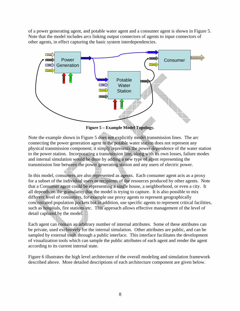
of a power generating agent, and potable water agent and a consumer agent is shown in Figure 5. Note that the model includes arcs linking output connectors of agents to input connectors of other agents, in effect capturing the basic system interdependencies.

ConsumerSatisfactionlWater

Comm

PowerGeneration

Fuel

Water

HRW

ind

Floo

d

Capa\city

Comm

PotableWaterStation

WaterHR

Win

d

Floo

d

Policy

Comm

Figure 5 – Example Model Topology.

Note the example shown in Figure 5 does not explicitly model transmission lines. The arc connecting the power generation agent to the potable water station does not represent any physical transmission component; it simply represents the power dependence of the water station to the power station. Incorporating a transmission line, along with its own losses, failure modes and internal simulation would be done by adding a new type of agent representing the transmission line between the power generating station and any users of electric power. In this model, consumers are also represented as agents. Each consumer agent acts as a proxy for a subset of the individual users or recipients of the resources produced by other agents. Note that a Consumer agent could be representing a single house, a neighborhood, or even a city. It all depends on the granularity that the model is trying to capture. It is also possible to mix different level of consumers, for example use proxy agents to represent geographically concentrated population pockets but in addition, use specific agents to represent critical facilities, such as hospitals, fire stations etc. This approach allows effective management of the level of detail captured by the model. Each agent can contain an arbitrary number of internal attributes. Some of these attributes can be private, used exclusively for the internal simulation. Other attributes are public, and can be sampled by external tools through a public interface. This interface facilitates the development of visualization tools which can sample the public attributes of each agent and render the agent according to its current internal state. Figure 6 illustrates the high level architecture of the overall modeling and simulation framework described above. More detailed descriptions of each architecture component are given below.

9

Figure 6 – Overall Model Architecture.

5.2 Scenario Preparation Tool A critical component of the architecture is support for automatically generating the structure of the model and subsequently generating execution scenarios. The Scenario Preparation Tool (SPT) is responsible for these two functions.

5.2.1 Model Generation Due to the large model size required for effectively simulating even a small region, generating the structure of the model must be done in a semi-automated manner. The proliferation of GIS data creates the opportunity of automatic conversion of such data into a model usable by the execution framework. Ideally, we would like to mine GIS data and generate agents, their attributes and linkages, in effect the total model. The accuracy of the model would be consistent with the accuracy of the GIS data, which is continuously improving. Work done in this project has demonstrated that even though this is a promising approach, numerous issues have to be addressed before it becomes practical. The primary issues are inconsistent attribution and concerns over confidential and/or proprietary data. Inconsistent attribution refers to the lack of consistent attributes associated with typical GIS data. For example, GIS layers with power distribution lines exist in various forms. However, there is

10

little, if any documentation on what the tags associated with these layers mean, and how such tags can be converted into useful for the model information. As an example, useful information may include the type of transmission line (kVA rating). In addition to lack of consistent attributes, topological information is often missing. For example, a transmission line may fan into two separate lines, something that would require a transmission or switching station, however, there is no matching data that provides information on that critical node of the system. After conducting numerous interviews with experts in the studied infrastructures, it became clear that the data required by the model is actually available. In keeping with the same example of power transmission and distribution lines, local utility companies have extensive data that describes the local utility grid. Such data is properly attributed, accurate and contains an extensive amount of additional cross reference information. Unfortunately, such data is considered proprietary and security critical, and thus unavailable for use in the project. Despite these limitations, the applicability of this modeling process can be demonstrated by using geo-typical data. Such data matches the overall layout suggested by GIS layers that are publicly available, but is not accurate enough to provide practical information about the region. Given that the scope of the project is limited to demonstrating a prototype, we did not consider this limitation to be critical, even though seeking such data expanded a significant amount of project resources. The model generation function of the SPT focused on utilizing as much of the GIS layers as possible, filling in typical data when necessary to provide a model that is comprehensive enough to demonstrate the modeling approach.

5.2.2 Generating Execution Scenarios. In addition to the model, a simulation requires specification of several configuration and input variables, such as time step and simulation duration. In addition, agent specific input parameters are provided if necessary. The SCP supports this function only once a model has been created, since such scenarios are model-specific. Agent-specific inputs are the primary means by which the default behavior of an agent can be overridden. This allows creating a variety of what-if scenarios that include various failure modes occurring during the simulation. Agent-specific inputs can be used in a power distribution agent, for example, to force a catastrophic failure at a specific point in the simulation. It can also be used to force a recovery following a simulated failure. On a technical basis, agent input parameters consist of time-event pairs, each pair dictating that an event will occur at the specific simulation time. Events consist of forced output values for any of an agent’s output connectors.

5.3 Agent-Based Model Execution Engine The execution engine is responsible for executing the model. For purposes of execution, the agent based model is viewed as a graph, whose nodes are represented by the agents and whose edges are the connections between agents. Agents have input and output connectors. Arcs connect connectors between different agents. Connectors are classified according to the

11

infrastructure they represent, so an input connector representing electrical power can only be connected to the output connector of an agent producing (or carrying) electrical power. This simple rule is enforced by assigning colors to each connector and requiring that edges only link connectors of the same color. The arcs then take on the color of their connectors. An example of an agent and its connectors is shown in Figure 7.

Waste Water

PumpingStation

Pressure

HR

Win

d

Floo

d

Comm.

Electric Power

Figure 7 – Connector Illustration.

Note that each agent can have multiple input and output connectors. An output connector can have any number of emanating arcs, but an input connector can only have up to one incoming arc. It is possible however to have an agent with multiple connectors of the same color. This constraint represents the fact that a given resource need cannot automatically be met by multiple providers. In the case of redundancy, for example a critical facility that is fed by two different electrical circuits, the model must include two input connectors. This approach forces the modeler to capture the redundancy and address the mechanics of its operation as part of the model. In the same example of the dual electrical feed, the modeler would have to address the redundancy by creating two different agents from where the dual feeds emanate, and possibly develop a model that represents the switch-over process that takes place when the primary feed fails. The following is a tentative list of arc classes.

a. Fresh water delivery pressure b. Electrical power c. Waste water recovery d. Human resources, represented as a percentage of capacity a. Communications, represented as availability of wireless signal 

The basic algorithm used for model execution is typical of graph based simulation models. Edges have values, representing the most recent value that was output by the source agent. Appropriate units, concrete or abstract can be associated with each arc. Each agent executes, reading its input connector values, and producing new values at its output connectors. This process continues until the end of the simulation.

12

The execution semantics are consistent with multi-rate discrete-time simulation, i.e., time advances by a fixed amount during each simulation step, but individual agents can run multiple iterations within each time step as required. It is also possible that an agent’s execution horizon is much larger than the simulation-imposed time-step, in which case an agent will simply maintain the same output over multiple time-steps. Note that use of continuous time semantics does not prevent the use of probabilistic discrete event model within each agent. Such an agent would maintain an internal event queue but wait before processing an event until that event’s time-stamp is greater than or equal to the external simulation time value. The execution engine operation is summarized below:

1) For each external infrastructure a. Isolate the infrastructure graph b. Generate the external model c. Execute the external model d. Import steady state data into the graph edges

2) Update current time 3) Capture a copy of all edge values 4) For each agent in the simulation

a. Call the execution function, providing arc values, current time and time-step 5) Gather data and update external connections

Step (1) is described in more detail in the following section. In effect, during this step, the external simulation(s) execute and pertinent results are imported back into graph, in the form of edge values. Steps (2)-(5) simply deliver the appropriate inputs to each agent and then execute all agents in an arbitrary order. Note that by capturing a copy of all input values before executing the agents, we eliminate any dependency between the order by which agents execute and the results.

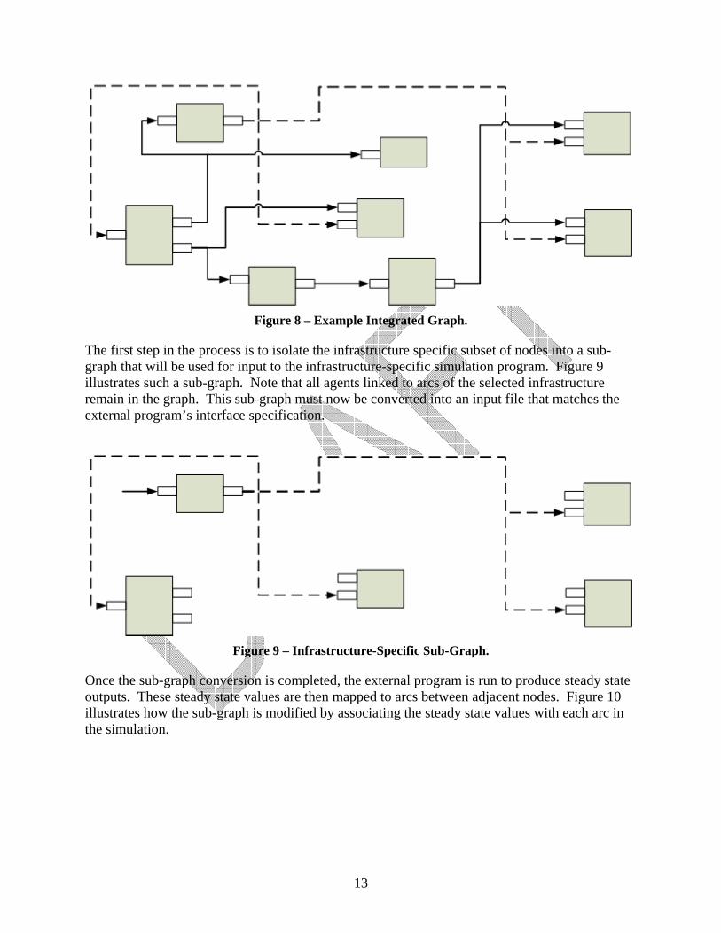
5.4 External Infrastructure Simulation The framework requires that the external infrastructure simulation program utilize infrastructure-specific information at a given simulation time in order to produce the steady state response of the system. In order to achieve this, after each time step, the framework isolates the part of the agent-based graph model that applies to the specific infrastructure and produces the appropriate input file. The external simulation program then executes the model producing steady state output for each link between nodes. As the last step in this process, the steady state values of the links are fed back to the integrated model. These values will then be used during the next time step by the internal models associated each agent. The process described above is better illustrated in a typical sequence. Figure 8 depicts an example infrastructure graph. For simplicity, only two types of infrastructures are included, as indicated by the type of arcs.

13

Figure 8 – Example Integrated Graph.

The first step in the process is to isolate the infrastructure specific subset of nodes into a sub-graph that will be used for input to the infrastructure-specific simulation program. Figure 9 illustrates such a sub-graph. Note that all agents linked to arcs of the selected infrastructure remain in the graph. This sub-graph must now be converted into an input file that matches the external program’s interface specification.

Figure 9 – Infrastructure-Specific Sub-Graph.

Once the sub-graph conversion is completed, the external program is run to produce steady state outputs. These steady state values are then mapped to arcs between adjacent nodes. Figure 10 illustrates how the sub-graph is modified by associating the steady state values with each arc in the simulation.

14

Figure 10 – Steady State Outputs Associated with Arcs.

Finally, Figure 11 illustrates the original graph but this time, arc values from the steady-state simulation are depicted with the corresponding arcs. At this point, the agent-based simulation can proceed for the next time step. Individual agents will utilize these values on their input connectors when performing their internal simulation.

Figure 11 – Original Graph With Steady State Arc Values.

5.5 ABM Communication Bus The ABM communication bus is an open interface that allows external tools to participate in the simulation. Participation can have many levels, passive, active and controlling. Passive participation implies that data can be received, but there is no interaction with the simulation. Active participation implies a bi-directional flow of data, where data can be requested by the simulation and is delivered by the external program. Finally, a controlling participation means that the external program can affect the simulation, by controlling the time advancement. Whereas time advancement can be considered an integral part of the simulation, providing an open interface that allows this function to be implemented outside the execution engine supports later expansion of the prototype tool.

15

The passive and interactive portions of the communication bus interface uses a publish-and-subscribe architecture. The communication bus enumerates available data streams and external programs can subscribe to these streams as needed. The only difference between the passive and interactive portions is the flow of data which can be bi-directional in the interactive portion. The controlling portion of the communication bus uses a client-server interface, with the remote program acting as a server and the engine active as the client. The engine makes service calls to the external program that replies as required. The interactions are time-synchronous, and can be used both for data delivery as well as time synchronization. To demonstrate the architecture, the prototype system incorporates a sample external program for each of the three levels. These tools are further described below.

5.5.1 Simulation Control The simulation control tool utilizes the controlling mode of operation. Its basic function is to provide the synchronization signal that advances the simulation. In addition, it provides a simple user interface that supports simulation pause, reset, single step execution and time-step control.

5.5.2 Visualization The visualization tool utilizes the passive mode of operation. Its primary function is to provide an immersive visualization of the simulated region. It is based on a software application that provides high quality baseline visualization of the terrain, buildings and basic infrastructure components, constructed from baseline GIS data. The tool loads the visual data associated with the region of interest and provides rudimentary eye-point control allowing the user to zoom in or move around the environment as needed. Figure 12 illustrates an example of a view created by the tool that is based entirely on GIS data.

Figure 12 – Baseline Visualization Example.

In addition to providing a baseline view of the region, the tool taps into the communication bus in order to display out-of-norm information associated with the various agents. The value of

16

each arc is compared to normal values and when an out-of-range condition is detected, the tool will highlight the associated visual element. The challenge in this approach is associating visual elements with specific simulation agents. The approach pursued by the project utilizes attributes in the GIS data used to create the original model, and depends on the visualization tool linking specific visual elements to those agents based on the attribute values. The ABM communication bus carries the attribute values, thus allowing the tool to link a particular agent, or arc, to the visual element. A demonstration of this approach is currently under development. The specific examples under consideration are the power lines and potable water delivery pipes.

5.5.3 Data collection The data collection tool is an example of the interactive level of operation. On one hand, the tool collects time-stamps of data available on the communication bus, but it can also deliver that data when necessary. One purpose for this would be to support pausing and re-winding a simulation. In the prototype demonstrator tool, the data collection saves all data in memory.