Embed Size (px)
Citation preview

Creating a Laser Produced X-ray Source
by
Phillip Bonofiglo
A honors thesis submitted in partial fulfillment of the requirements for the Honors PhysicsBachelors of Science degree at the University of Michigan 2013
Thesis Advisor: Dr. Carolyn Kuranz


I would first like to thank my thesis advisor, Dr. Carolyn Kuranz, for all her help in writingthis thesis. I would then like to thank Dr. Paul Keiter and Dr. Paul Drake for overseeing my
research and introducing me to the wonderful field of HED physics. In addition, manythanks are owed to Mariano, Sallee, Caleb, Chris, and Thomas for all of their hard work andhelp in making this project come together. Lastly, I would like to thank all of my friends and
family for all their support and for making me a better person and physicist.
ii

Table of Contents
DEDICATION . . . . . . . . . . . . . . . . . . . . . . . . . . . . . . . . . . . . . . . . . . . . . . . . ii
LIST OF FIGURES . . . . . . . . . . . . . . . . . . . . . . . . . . . . . . . . . . . . . . . . . . . . iv
ABSTRACT . . . . . . . . . . . . . . . . . . . . . . . . . . . . . . . . . . . . . . . . . . . . . . . . . v
CHAPTERS
Introduction . . . . . . . . . . . . . . . . . . . . . . . . . . . . . . . . . . . . . . . . . . . . . . . . . 11 Introduction to High-Energy-Density Physics . . . . . . . . . . . . . . . . . . . . . . . . . . . 22 Plasma X-ray Interactions . . . . . . . . . . . . . . . . . . . . . . . . . . . . . . . . . . . . . . 33 Creating an X-ray Source . . . . . . . . . . . . . . . . . . . . . . . . . . . . . . . . . . . . . . 44 X-ray Radiography . . . . . . . . . . . . . . . . . . . . . . . . . . . . . . . . . . . . . . . . . . 6
Experimental Setup . . . . . . . . . . . . . . . . . . . . . . . . . . . . . . . . . . . . . . . . . . . . . 91 Alignment and Setup . . . . . . . . . . . . . . . . . . . . . . . . . . . . . . . . . . . . . . . . . 92 Vacuum Assembly . . . . . . . . . . . . . . . . . . . . . . . . . . . . . . . . . . . . . . . . . . 123 Target Design . . . . . . . . . . . . . . . . . . . . . . . . . . . . . . . . . . . . . . . . . . . . . 134 Diagnostics . . . . . . . . . . . . . . . . . . . . . . . . . . . . . . . . . . . . . . . . . . . . . . 145 Spot Size . . . . . . . . . . . . . . . . . . . . . . . . . . . . . . . . . . . . . . . . . . . . . . . 15
Limiting Experimental Factors . . . . . . . . . . . . . . . . . . . . . . . . . . . . . . . . . . . . . . 171 Spherical Aberrations in the OAP . . . . . . . . . . . . . . . . . . . . . . . . . . . . . . . . . 172 Manufactured Faults in the OAP . . . . . . . . . . . . . . . . . . . . . . . . . . . . . . . . . . 203 CCD Resolution . . . . . . . . . . . . . . . . . . . . . . . . . . . . . . . . . . . . . . . . . . . 224 Conclusion . . . . . . . . . . . . . . . . . . . . . . . . . . . . . . . . . . . . . . . . . . . . . . 24
Results . . . . . . . . . . . . . . . . . . . . . . . . . . . . . . . . . . . . . . . . . . . . . . . . . . . . . 251 Determining a X-ray Signal . . . . . . . . . . . . . . . . . . . . . . . . . . . . . . . . . . . . . 252 Characterizing the X-ray Signal . . . . . . . . . . . . . . . . . . . . . . . . . . . . . . . . . . . 27
Conclusion . . . . . . . . . . . . . . . . . . . . . . . . . . . . . . . . . . . . . . . . . . . . . . . . . . 301 Future Work . . . . . . . . . . . . . . . . . . . . . . . . . . . . . . . . . . . . . . . . . . . . . 302 Concluding Remarks . . . . . . . . . . . . . . . . . . . . . . . . . . . . . . . . . . . . . . . . . 32
Appendix A . . . . . . . . . . . . . . . . . . . . . . . . . . . . . . . . . . . . . . . . . . . . . . . . . . 33A.1 . . . . . . . . . . . . . . . . . . . . . . . . . . . . . . . . . . . . . . . . . . . . . . . . . . . 33A.2 . . . . . . . . . . . . . . . . . . . . . . . . . . . . . . . . . . . . . . . . . . . . . . . . . . . 36
Appendix B . . . . . . . . . . . . . . . . . . . . . . . . . . . . . . . . . . . . . . . . . . . . . . . . . . 37
References . . . . . . . . . . . . . . . . . . . . . . . . . . . . . . . . . . . . . . . . . . . . . . . . . . . 42
iii

List of Figures
1.1 Temperature vs. Density for a system in the HED regime2 . . . . . . . . . . . . . . . . . . . . 21.2 Schematic of Backlighting Scheme (Not drawn to scale)6 . . . . . . . . . . . . . . . . . . . . . 51.3 X-ray Radiograph of a Radiative Shock4 . . . . . . . . . . . . . . . . . . . . . . . . . . . . . . 61.4 Diagram of a Pinhole Camera19 . . . . . . . . . . . . . . . . . . . . . . . . . . . . . . . . . . . 71.5 Schematic of Magnification vs. Field of View . . . . . . . . . . . . . . . . . . . . . . . . . . . 82.1 General schematic of experimental design
† Optics lie within dashed box. Further detail in Figure 2.3 . . . . . . . . . . . . . . . . . . . 92.2 Basic diagram for an OAP20 . . . . . . . . . . . . . . . . . . . . . . . . . . . . . . . . . . . . . 102.3 OAP Alignment Schematics . . . . . . . . . . . . . . . . . . . . . . . . . . . . . . . . . . . . . 102.4 Basic layout of CCD, linear stage, and target mount . . . . . . . . . . . . . . . . . . . . . . . 112.5 Picture of vacuum chamber assembly . . . . . . . . . . . . . . . . . . . . . . . . . . . . . . . . 122.6 Picture of components that go in chamber with target in place . . . . . . . . . . . . . . . . . 132.7 Target Schematic . . . . . . . . . . . . . . . . . . . . . . . . . . . . . . . . . . . . . . . . . . . 143.1 Ray diagram showing sagittal, tangential, and best foci . . . . . . . . . . . . . . . . . . . . . 183.2 Coma14 . . . . . . . . . . . . . . . . . . . . . . . . . . . . . . . . . . . . . . . . . . . . . . . . 193.3 Actual picture of focused Nd:YAG spot . . . . . . . . . . . . . . . . . . . . . . . . . . . . . . 203.4 Ray diagram of light scattering off an uneven surface23 . . . . . . . . . . . . . . . . . . . . . . 213.5 Spot on pixels of equal size27 . . . . . . . . . . . . . . . . . . . . . . . . . . . . . . . . . . . . 22
3.6 Spot on pixels of1
3the size27 . . . . . . . . . . . . . . . . . . . . . . . . . . . . . . . . . . . . 23
4.1 Radiograph of First Shot with 250 µm Au . . . . . . . . . . . . . . . . . . . . . . . . . . . . . 264.2 Radiographs of 150 pulse bursts with 250 µm Au . . . . . . . . . . . . . . . . . . . . . . . . . 264.3 Diagrams of Stepped Al and Film Bundle . . . . . . . . . . . . . . . . . . . . . . . . . . . . . 274.4 Radiographs with Al steps and Au . . . . . . . . . . . . . . . . . . . . . . . . . . . . . . . . . 284.5 Radiograph with Al steps and Background Radiograph . . . . . . . . . . . . . . . . . . . . . . 28
iv

ABSTRACT
Creating a Laser Produced X-ray Source
by
Phillip Bonofiglo
The principal aim of high-energy-density (HED) physics is to understand systems at extreme pressures
and temperatures. The extreme nature of HED events, however, makes diagnosing them very hard. X-ray
backlighting is an important tool in diagnosing many high-energy-density experiments. X-rays produced from
irradiated metal foils are used to probe plasmas and determine plasma density, composition, and structure.
This process is called x-ray backlighting and often suffers from low signal-to-noise and low conversion efficiency.
The conversion from laser energy to x-rays, via the irradiation of a solid metal target, has been shown to be a
complex process with often inconsistent results.
In the work of this thesis, we strive to produce and detect the x-ray signal created in backlighting.
We will study laser-irradiated metal foils with a low-energy laser. A Nd:YAG laser will be employed to
irradiate a 5 µm thick Ti metal foil. This thesis will present our initial design work on the experimental setup
and will also report our first measurements of the x-ray signal from the Ti irradiated foils from a photodiode
and x-ray sensitive film. As a part of this thesis, the basic underlying physical principles of the experiment
will be explained, along with the experiment’s main sources of error and uncertainty. Our future work will
entail improving the experimental setup and strengthing the signal already achieved.
v

CHAPTER: 1
Introduction
The work of this thesis is inspired by past and current work in the field of High-Energy-Density
(HED) physics. HED physics is the regime in which pressures are in excess of one million atmospheres.
HED physics is commonly thought of as a sort of plasma physics. This simplification is not entirely correct.
Much of traditional plasma theory does not describe HED physics. Instead, one must refer to a theory of
denser plasmas.1 These extremely high temperature, greater than 100 million degree Kelvin, or high pressure
systems are often re-created in the lab.1,2,3,4,5,6,7,8,9,10 The properties and laws that govern HED physics
can allow for an accurate scaling of the observed micron-sized phenomena to those produced in astrophysical
events.4,6,7
Many of these events are re-created using high-energy lasers, such as the OMEGA laser facility at the
University of Rochester or the National Ignition Facility at Lawrence Livermore National Laboratory.11,12 The
HED events that inspired the work of this thesis are those conducted by the Center for Laser Experimental
Astrophysics Research (CLEAR) at the University of Michigan. The events studied primarily include
hydrodynamic instabilities, such as: Kelvin-Helmholtz instabilities, Rayleigh-Taylor instabilities, Richtmeyer-
Meshkov instabilities, radiative shocks, and other astrophysically relevant phenomena.4,6,7,8 One of the
diagnostic techniques used to observe these events is x-ray radiography. X-ray radiography is a process that
involves irradiating a metal foil to create x-rays to produce an image. The experiment outlined in this thesis
is strongly related to x-ray radiography and backlighting on a smaller energy scale than that achieved at
high-energy laser facilities. The work, herein, strives to produce and characterize backlighting in the lab with
the use of a low-energy, table-top laser.
I will start with an introduction to HED physics and x-ray radiography and highlight any background
information needed to understand the concepts, designs, errors, and results of our work. I will then describe
the experimental setup in detail, describing alignment and focusing of the laser and the diagnostics used.
I will then follow the experimental setup by discussing the design flaws inherent to our system that limit
the quantitative analysis we can perform on the laser spot and x-ray signal. The results of our work will be
presented and will discuss the initial x-ray production and characterization. I will then conclude this thesis
with remarks on the merit of the experimentation and an outlook on future work.
1

1 Introduction to High-Energy-Density Physics
The HED regime can be described when the energy density of a system corresponds to a pressure
greater than one million atmospheres (1Mbar, 0.1 TPa).1,2 Thus, a system can be in the HED regime due to
thermal pressure, intense electric or magnetic fields, large internal energies, or a combination of those.2 Many
systems can be described as HED. Some common HED systems can include strong magnetic fields, intense
laser fields, intense x-ray radiation, and particle beams. In fact, there is a strong correlation to particle
physics, as many particle beams are in the HED regime.2
When one crosses the million atmosphere mark, one does not simply enter into a new regime of
physics described by a single set of equations or theories. In fact, the HED regime is highly structured and
organized based on the total energy density for a given system.
Figure 1.1: Temperature vs. Density for a system in the HED regime2
Looking at Figure 1.1, everything to the right of the line labeled 0.1TPa is in the HED regime. At
sufficiently high temperatures, the system is in a relativistic state in which the electrons are highly energetic
and move at such velocities that their kinetic energy exceeds their rest masses. The section labeled “Radiative
plasma” describes the region in which the plasma can radiate. The resulting energy loss of the system from
radiation is then large enough to alter strucutre and behavior. The section labeled “Nonideal plasmas” simply
describes the area where traditional plasma theory fails. The parameter, Γ, in the figure is the ratio of
electrostatic to thermal energy. As the two become comparable, the plasma enters a strongly coupled and
degenerate state. The electrons, therefore, need to be described as fermions, and Coulomb and quantum
mechanical effects need to be strongly considered. In summary, by looking at the plot above, one can clearly
2

see that HED physics is a highly complex field.
2 Plasma X-ray Interactions
To probe these intense systems, a wide array of diagnostics is available. Some diagnostics typically
used include: streak cameras, various spectrometers, and framing cameras. The dense plasma created in
many HED events, such as those studied by CLEAR, are completely invisible in the optical spectrum. The
frequency at which light can interact with the plasma is determined by its plasma frequency, ωp:13,14
ωp =
√4πq2npγme
(1.1)
where np is the plasma density, γ is the relativistic lorentz factor given by the electrons in the plasma, and
me is the mass of an electron. Any frequency below the plasma frequency is blocked by the plasma, and the
light-plasma interactions mimic that of a conductor.13 For many plasmas studied in laboratory astrophysics,
the plasma frequency is greater than the visible spectrum. Therefore, x-rays are often used to probe the
plasma. X-ray radiography is a technique that uses x-rays to capture an image onto a detector.5,8
One useful aspect of x-ray radiography is that x-ray measurements can yield opacities, which can
infer densities of the plasma, if the thickness of the plasma is known.4,6,7,15 To do this, one can apply the
Beer-Lambert equation:15
T =I
I0= e−σρl = e−τ (1.2)
where T is the transmission of x-rays through the material, I is the intensity of x-rays transmitted, I0 is
the original x-ray intensity, σ is the mass attenuation coefficient, ρ is the density of the material, l is the
thickness of the material, and τ = σρl is the opacity. Therefore, the transmission of a given x-ray decreases
exponentially as the material’s opacity increases. It is relatively simple to see this relation. Imagine a photon
incident on some material. The photon penetrates the material and interacts with the nuclei. The thicker or
denser the material, the more likely the photon is to be completely absorbed by a single atom or scattered by
many atoms to the point where the photon has given up all of its energy to the nuclei. This is why thick,
dense materials, such as lead, are used to block x-rays. Therefore, for a given opacity, one will observe an
increase in transmission with an increase in photon energy.
The Beer-Lambert equation works both ways. That is, given a known x-ray energy or transmission
and thickness of the material, the density of the material or plasma can be found and vice versa. In the
3

work of this thesis, we will exploit the latter. A x-ray sensitive film with different elemental filters will be
used to analyze the x-ray spectrum produced. The known K-edge of the metals will be exploited to create
certain bands in transmission in order to look at the x-rays of primary interest. The Center for X-ray Optics
at Lawrence Berkeley National Lab has made an applet that finds the transmission of a specified x-ray
range through a specified material, given its density and thickness.15 There measurements are based off of
experimental results and theoretical calculations in regions with little experimental data. This source was
used often in calibration of our x-ray spectrum and serves to demonstrate the usefulness of the Beer-Lambert
equation.
3 Creating an X-ray Source
As mentioned earlier, backlighting is when a laser irradiates a thin metal foil to create x-rays for
diagnostic purposes.4,6,7,8,9,10,16 These x-rays are behind the main experiment and provide a backlit signal to
observe the main events of interest. Hence, the name backlighting. These backlit x-rays probe the plasma and
are transmitted or absorbed depending on the plasma density, as described in the previous section, see Eqn.
(1.2). The two signals of typical interest in HED experiments are often the He-alpha like line (1s2p→ 1s2
transition) and the Kα line (2p→ 1s transition).7 The two signals are produced in two different ways and
are dependent on the irradiance achieved by the laser.9,10,17
When the focused laser is incident on the foil, it creates a plasma on the surface of the foil. The
atoms on the front of the foil become highly ionized and retain only one, two, or a few electrons. Many of
these atoms are He-like and give off x-rays from the 1s2p→ 1s2 transition.7 Hence, the name He-alpha like.
For high irradiances, ∼ 1015 − 1023W/cm2, electrons liberated from the front surface of the foil have enough
energy to penetrate into the denser back end of the foil.9,17 The ionized electrons knock out inner-shell
electrons from the back end of the foil creating Kα emission. These two processes create discrete lines in the
produced x-ray energy spectrum. Brehmstralung radiation is also created in the process as some electrons
are decelerated by the surroundings, providing a continuous spectrum. A desired signal can then be obtained
by filtering one’s diagnostics, using the Beer-Lambert equation and known elemental filters. It is worthy
to note, that some of the energetic electrons ionized from the front end of the foil are repelled away from
the back end of the foil due to the induced electric field created by the other electrons.2 These repulsed,
highly energetic, electrons can often produce noticeable background noise in one’s x-ray spectrum or other
diagnostics. This is not the case for our experiment because of the low energies used, but “hot” electrons do
need to be considered at higher energies. It is also wothwhile to mention that the creation of x-rays occurs on
order of the pulse length of the laser. Thus, for our experiment, the x-ray production occurs in nanoseconds.
For our experiment, the main signal of interest is the He-alpha like line of Ti at 4.71 keV. The Kα
4

line at 4.51 keV requires higher irradiances than our laser and focusing optics can achieve and cannot be
induced by our setup. For an irradiance of ∼ 1013 − 1015W/cm2, the He-alpha like transition should be the
signal of highest intensity created. Backlighting exploits this fact. At low irradiances, the metals chosen for
backlighters are chosen based on their He-alpha like lines and the signal needed for experimentation.
There are two main types of backlighters: area and pinhole. Area backlighters are simply just a flat
piece of metal.8,18 A laser irradiates the metal foil and x-rays are produced at a solid angle of 4π steradians.
However, a slightly larger x-ray signal will be detected from the plume of plasma created normal to the
surface of the foil in the direction of the oncoming laser radiation. As there is no clear directionality to
area backlighters, they are often positioned close to targets to illuminate them more. The second type of
backlighter is the pinhole backlighter. A pinhole backlighter is composed of three parts: a large background
foil with a hole (often tapered) in its center, a piece of plastic placed just above the background foil to act as a
damping agent against oncoming plasma flow, and a small metal foil chosen for its He-alpha like emission.5,6
The small metal foil is what is going to be primarily irradiated by the laser and create the x-ray signal. The
small foil is placed on the plastic right in front of the hole on the background foil. The small foil is irradiated
with the laser, a plasma plume is created, and x-rays are produced. Some of the x-rays are transmitted
through the hole in the background foil and are transmitted in a conic shape, as seen in Figure 1.2.
(a) Sideview of backlighting scheme (b) Backlighter face
Figure 1.2: Schematic of Backlighting Scheme (Not drawn to scale)6
The pinhole backlighter has much more directionality than the area backlighter, and the angle of
projection from the hole can be altered by the size of the pinhole or its taper. Therefore, pinhole backlighters
can be used at larger distances than area backlighters. The x-rays produced from these backlighters then fall
onto an object and are absorbed or transmitted, depending on the object’s properties. A detector is placed
on the other side of the object and the transmission of x-rays is recorded, producing an image on the detector.
5

This technique is called x-ray radiography and will be discussed next.
4 X-ray Radiography
While our experiment does not perform x-ray radiography, x-ray radiography still needs to be
discussed. X-ray radiography is the basis for our current research and is the goal for our future work. X-ray
radiography is the motivation for our experiment and serves to demonstrate one of the diagnostic techniques
used in HED physics.
Looking back at Eqn. (1.1), one can see that the frequency at which the plasma can be probed
depends on the plasma density. Like most materials, the density of the plasma strongly relates to how
much the x-rays are absorbed or scattered. A denser plasma absorbs higher energy x-rays and a less dense
plasma absorbs less of the same energy, for the same thickness. Therefore, one can determine the density
and structure of plasmas, or x-ray energy, by looking at the opacity of the materials in x-ray radiographs, as
mentioned before.
Looking at Figure 1.3, we see an x-ray radiograph of a radiative shock recorded on x-ray sensitive
film. The block above the tube and shock is a stepped piece of aluminum. The thicknesses of the steps are
known precisely and are used as a standard to help determine the the spectrum of the x-ray source. Using
known materials and Eqn. (1.2), we can determine the opacity of the plasma. So, it is evident that different
plasmas, depending on their density and thickness, will respond to different x-ray signals. The advantage of
x-ray radiography is that if one needs a different x-ray signal to probe a certain plasma, then all one needs to
do is change the metal they are irradiating. Each metal will have its characteristic He-alpha and He-beta
lines to probe the plasma at different energies.
Figure 1.3: X-ray Radiograph of a Radiative Shock4
6

The two backlighters described in the previous section are the main components of x-ray radiography,
along with the detectors. The closest analogy to backlighting is a pinhole camera. In a pinhole camera, light
is emitted from an object, travels through the pinhole (in the familiar conic shape one gets when light travels
through a small aperature) onto a film or detector, and produces an inverted image. A diagram for a pinhole
camera can be seen in Figure 1.4. A pinhole backlighter simply switches the light source and image and
places a target between the image plane and source. A area backlighter has a pinhole on the detector to
capture light and follows a pinhole camera directly. When discussing the produced image, two main factors
to consider are magnification and resolution.
Figure 1.4: Diagram of a Pinhole Camera19
The magnification of an image can be given in terms of the ratio of its image size to object size, hi
ho,
or image distance to object distance, dido
.14 It’s very easy to set the magnification of one’s image because
one already knows the object size and is free to vary the image distance and object distance to find the
desired image size. This corresponds to simply moving the target and backlighter to suitable positions that
provide the needed magnification (or moving the pinhole camera closer or farther from the object, using
a more familiar concept). A small caveat, however, is that the distance the target and backlighter can be
placed is limited by the size of the laser chamber and facility flexibility. For a ∼ 1mm HED experiment,
it is often the practice to use a magnification of 10-20X for a given size detector. The main setback with
increasing magnification is that the field of view shrinks for a given detector size. Looking at Figure 1.5, as
one increases the magnification, ( dido ), the circular cross-section that lies in the target plane decreases.14 This
cross-section corresponds to the amount of target seen, i.e. the field of view.
The resolution of one’s image is ultimately determined from the size of your pinhole.16 In the
Fraunhoffer limit, when r >> λ, the light that propagates through the pinhole will form an Airy’s pattern.
This is always true for backlighting setups, as x-rays are on the order of Angstroms. The smallest resolution
7

(a) Small Magnification, Large FOV (b) Large Magnification, Small FOV
Figure 1.5: Schematic of Magnification vs. Field of View
one will achieve is when two Airy’s disks start to overlap. This distance is given by:14
d = 2.44λf
D(1.3)
where λ is the wavelength of light, f is the focal length (distance from object plane to image plane), and D is
aperture size (diameter of the pinhole). Thus, for fixed distances and λ, the spatial resolution obtained in
the image is determined by the size of the pinhole. Keeping the magnification fixed, to increase the spatial
resolution one must decrease the size of the pinhole aperture. The down side to decreasing pinhole size is
decreasing the amount of signal transmitted.16 As, the pinhole gets smaller, fewer x-rays are transmitted
through the aperture, decreasing the signal recorded by the detector. The signal transmitted is proportional
to the area of the pinhole, so simply changing the pinhole from 10 µm to 5 µm will decrease the signal by a
factor of 4. Furthermore, the cone of emitted x-rays becomes smaller, decreasing the angular resolution and
field of view, as well.16
As one can see, there are many trade offs to choosing an increased magnification or spatial resolution.
Often, the main limiting factors are the size of the laser facility and the characteristics in the image that
need to be resolved. The choice between area and pinhole backlighter needs to be made, and the metal foils
to create the x-ray signal need to be determined. Overall, x-ray radiography is relatively simple in practice
but many details need to be sorted out to insure a high-quality image is produced.
8

CHAPTER: 2
Experimental Setup
As described earlier, backlighting is a relatively simple process that involves the irradiation of a
thin-metal foil with a high-energy laser. An x-ray source was re-created in the lab using a small table-top
Nd:YAG laser (532 nm wavelength, 8 ns pulse, 160 mJ pulse, 6 mm beam diameter) to irradiate Ti foils
under vacuum. The produced x-rays were then observed and measured using a photodiode and x-ray sensitive
film. The Nd:YAG laser was aligned using two, low power, HeNe lasers and various optical components.
The Nd:YAG laser was focused using an off-axis parabolic mirror (OAP) onto either a Hitachi KP-D20BU
CCD camera, to measure the beam spot size, or a thin-metal foil to create x-rays. A basic schematic of the
experimental setup can be seen in Figure 2.1.
Figure 2.1: General schematic of experimental design† Optics lie within dashed box. Further detail in Figure 2.3
1 Alignment and Setup
Alignment of the main laser beam was accomplished in two stages. The first stage involved alignment
of the OAP, and the second stage involved finding the focal spot of the OAP. The OAP has a 50.8 mm
effective focal length, 25.4 mm parent focal length, 20.54 base diameter, and has an aluminum surface. A
basic diagram for an OAP is shown below.
9
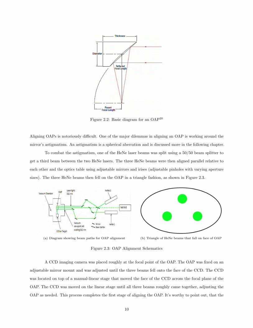
Figure 2.2: Basic diagram for an OAP20
Aligning OAPs is notoriously difficult. One of the major dilemmas in aligning an OAP is working around the
mirror’s astigmatism. An astigmatism is a spherical aberration and is discussed more in the following chapter.
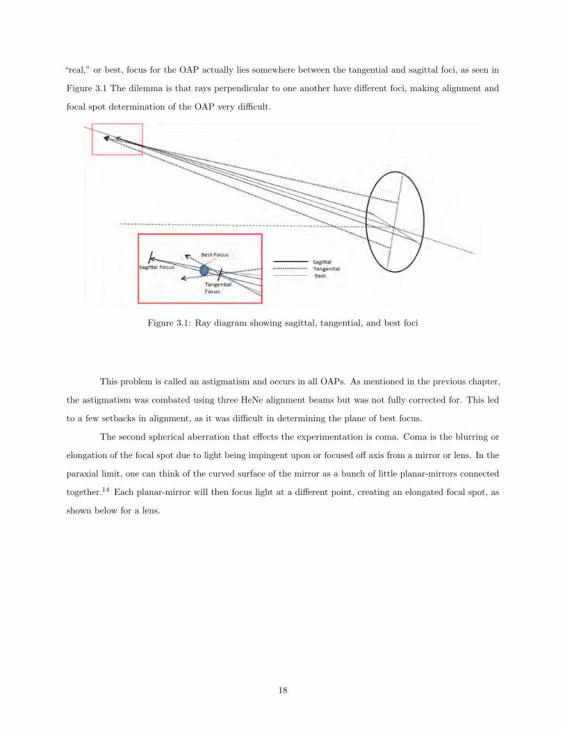
To combat the astigmatism, one of the HeNe laser beams was split using a 50/50 beam splitter to
get a third beam between the two HeNe lasers. The three HeNe beams were then aligned parallel relative to
each other and the optics table using adjustable mirrors and irises (adjustable pinholes with varying aperture
sizes). The three HeNe beams then fell on the OAP in a triangle fashion, as shown in Figure 2.3.
(a) Diagram showing beam paths for OAP alignment (b) Triangle of HeNe beams that fall on face of OAP
Figure 2.3: OAP Alignment Schematics
A CCD imaging camera was placed roughly at the focal point of the OAP. The OAP was fixed on an
adjustable mirror mount and was adjusted until the three beams fell onto the face of the CCD. The CCD
was located on top of a manual-linear stage that moved the face of the CCD across the focal plane of the
OAP. The CCD was moved on the linear stage until all three beams roughly came together, adjusting the
OAP as needed. This process completes the first stage of aligning the OAP. It’s worthy to point out, that the
10

triangle shaped beam design does not fully solve the astigmatism problem. In fact, there is no point at which
all three beams coalesce because all three beams have different foci. This method was used to provide a quick
alignment of the OAP and provide a rough estimate of the best focus. The more important determination is
that of the best focus for the Nd:YAG laser itself.
Determining the focal point of the Nd:YAG beam is of critical importance because the laser pulse
will only reach intensities high enough to create x-rays if the focal point is on the order of several microns.
The Nd:YAG focal point was found by first aligning the Nd:YAG beam along one of the same beam paths as
one of the HeNe beams, as shown in Figure 2.3. Removing the beam splitter and a couple mirrors, a straight
shot for the Nd:YAG pulse to enter the vacuum chamber was made. The HeNe path was found by placing
two irises on the straight part of the HeNe’s path. The Nd:YAG was then adjusted so that it passed through
the same two irises. This insures that the Nd:YAG beam followed the same vector as the HeNe beam prior to
entering the chamber, and will, thus, follow the same path as the HeNe beam inside the chamber. With the
Nd:YAG beam following the same trajectory as one of the HeNe beams, the Nd:YAG will fall onto the CCD
just as the HeNe and will be roughly in focus. Neutral density filters were then inserted in the beam path to
lower the intensity of the laser light that fell on the CCD and protect it from damage. The CCD was then
moved back and forth across the focal point until the smallest spot was observed. This point was taken as
the best focus for the Nd:YAG beam. The CCD-linear-stage assembly can be seen in Figure 2.4.
Figure 2.4: Basic layout of CCD, linear stage, and target mount
When performing the actual experiment, the CCD is removed and the target is set in place to lie in
the plane of the CCD itself. More on this procedure is described in section 2.3.
11

2 Vacuum Assembly
The vacuum chamber is a standard 6-way cross with CF-flanges. All 6 flanges are 8” in diameter,
and the total length across the cross is 13” in all x, y, and z directions. An overview of the vacuum system
can be seen in Figure 2.5. The chamber is initially pumped down to a rough vacuum, ∼ 20 mTorr, using
Figure 2.5: Picture of vacuum chamber assembly
Agilent’s Tri-Scroll pump, then pumped down to a fine vacuum, ∼ 10−6 Torr, using a Pfeiffer HighPace turbo
pump. The flange incident to the incoming laser light has a viewport installed with a 532 nm anti-reflective
coating to minimize power loss. The flange directly opposite of the viewport has a 90 degree flange bent
downward that connects the turbo pump to the system. The top flange has a 8” - 2.75” converter flange that
holds a custom housing for a photodiode. The photodiode is read by a Kingsley 2002 Multimeter via a BNC
cable vacuum feed-through. The bottom flange has a 8” - 2.75” converter flange fitted with an ion pressure
gauge. Facing the viewport, the flange to the left is closed with a blank 8” flange, and the flange to the right
has a 8” - 2.75” converter flange and a 2.75” to 1/4” male NPT converter that holds a spring loaded pressure
relief valve. The pressure relief valve is set to open at just above atmosphere when pumping up the chamber
to atmosphere.
Inside the chamber, there is large plate that runs across the entire length of the chamber from left to
right, when facing the viewport. Mounted on the plate are the linear stage on which the CCD and target
mount lie and another linear stage on which the OAP sits. The OAP is centered on the right side of the
viewport and is placed such that incoming light reflects 90 degrees to the left, toward the CCD/target. The
CCD linear stage traverses along the reflected beam path (i.e. along the plate) and the mirror linear stage
12

traverses perpendicular to that. The CCD linear stage is used in finding the focal point of the OAP, as
described earlier, and the mirror linear stage is used to move the beam spot horizontally across a target. By
moving horizontally across the face of a target, the spot on the target being irradiated can easily be changed
from shot to shot. This allows for quick turn over time between shots. There is no apparatus to hold the
film. The film leans against the mirror mount facing the target. A diagram of all the components inside the
chamber can be seen in Figure 2.4, and a picture of the components, minus the CCD, can be seen in Figure
2.6.
Figure 2.6: Picture of components that go in chamber with target in place
3 Target Design
The target is simple in design and is characteristic of simple area backlighters.8,18 The base of the
target is an aluminum mount with two fitted magnets on its bottom. These magnets connect the target to
the target mount and hold it into place. The length of the target is determined from where the focal spot is
found. When the focal spot is found on the CCD, the distance to the base of the target mount to the back of
the CCD housing is measured, and the distance from the back of the CCD housing to the plane of the CCD
is available from the manufacturer’s schematics. The length of the target is then produced to the total length
from the base of the target mount to the face of the CCD using these measurements. The target foil then lies
in the plane of the CCD and, thus, the focal spot of the laser beam found earlier. The target is composed of
a tungsten carbide stalk and a thin metal foil. The tungsten carbide stalk is inserted into the center of the
aluminum mount and cut to the desired length. The metal foil is then attached orthogonally to the stalk as
13

shown in Figure 2.7 using a UV cure glue. With the foil orthogonal to the stalk, the incident laser will also
be orthogonal, or nearly orthogonal, to the foil.
(a) Target Design (laser comes from right to irradiate foil) (b) Target Design (irradiated face)
Figure 2.7: Target Schematic
The foil chosen for experimentation was 5 µm thick Ti and was cut to be 5 mm x 5 mm. The Ti foil was
attached to the end of the stalk using micron-precise motorized linear and rotational stages.
4 Diagnostics
There were two primary diagnostics to analyze the x-rays produced: a photodiode and x-ray sensitive
film. The photodiode is the AXUV 100 made by Opto Diode Corp. and is a Si p-n junction photodiode. For
wavelengths shorter than 1100 nm, electron-hole pairs are created, via the inner photoelectric effect, for every
3.6 eV. The electrons and holes are separated by the electric field created by the p-n junction and create a
current proportional to the number of electron-hole pairs created. The current produced from the photodiode
is used to detect the presence of x-rays and the overall flux of the x-rays produced. Two advantages of the
AXUV 100, however, are that it has no dead zone and a thin protective entrance window.21 No dead zone,
implies that there is no region in which electron-hole pairs will recombine. Thus, 100% of electron-hole
pairs created will be observed in the current reading. The thin entrance window insures no reflection and
absorption of photons, except in the 7 - 100 eV range. Therefore, most photons in the x- ray range will be
absorbed by the silicon diode, depending on Si thickness, and the quantum efficiency of the photodiode can
be approximated accurately as:21
QE =Eph3.6
(2.1)
14

where QE is the quantum efficiency and Eph is the photon energy in eV. To block visible light, 25 µm black
Kapton was placed in front of the photodiode to insure only x-rays were detected.
The x-ray sensitive film used is composed of a polyethylene terephtalate substrate with an emulsion
layer of cubic silver halide crystals (99% AgBr, 1% AgI).22 When x-rays are incident on the silver halide
crystals, electrons from the crystal are ejected via the photoelectric effect and become trapped close by in
“sensitivity sites.” The electrons interact with the silver ions and form a metallic silver and a latent image.
The image can then be recovered using chemical reactions in development. The sensitivity and resolution of
film is therefore based on the crystal structure and amount of silver halide.22
The x-ray sensitive film available was AGFA D8 and D7 film.18,22 D7 is less sensitive to x-rays than
the D8 film by a factor of 1.7 and has yet to be used in our experimentation. Only the more receptive D8
film has been used. The film was packaged in 25 µm thick black Kapton that is opaque to visible light and
transparent to x-rays of energies above ∼ 1 keV. The film was packaged as a 1” circle and had a 250 µm
thick gold foil placed on half of it. The gold acts as shielding and blocks all incident x-rays, creating a step
in absorption, as seen on the film. Other metal filters were used in this manner in characterizing the x-ray
signal. This will be discussed more in the results portion of this thesis.
5 Spot Size
The spot size was measured using the CCD and the Python Script in Appendix A.1. The KP-D20BU
CCD is a video camera and only records video, so video of the beam spot is taken during the last steps of the
process outlined in section 2.1. The video is captured via a software called VeeDub and is saved as a .avi file.
A frame corresponding to the Nd:YAG focal spot is taken from the .avi file and converted to a .png to be
read by the Python code.
The code displays to the user a 2-D image of the beam profile and prompts the user for the pixel
value for the mid-line of the beam spot. The code then takes a line-out of the image at the user specified
pixel number and stores the pixel values in an array. An intensity profile of the line is then plotted from
the line-out and the FWHM is calculated and plotted across the intensity profile. The FWHM is defined as
half-way between 95% and 5% of the maximum pixel value. The code then asks the user for the number of
pixels in the FWHM that lie within the intensity profile. The spot size is then calculated by multiplying the
number of pixels that lie within the FWHM by the pixel size and some conversion factor. The conversion
factor is necessary, as the true pixel size of the CCD is lost when the image is converted to a digital form.
The conversion factor was found by using the code to measure a beam of known width. A sample intensity
profile for an alignment laser spot can be seen in Appendix A.2.
The theoretical spot size can be determined from the limit of resolution between two Airy disks.
15

This familiar formula in optics was given in Eqn. (1.3). For a 532 nm wavelength, focal length of 50.8 mm,
and a 6 mm aperture size, one finds the diffraction limited spot size to be on the order of 10 microns. We can
find the theoretical intensity of our laser spot with:
I =E/t
πr2(2.2)
where I is the intensity, E is the pulse energy, t is the pulse length, and r is the spot radius. The intensity of
the Nd:YAG laser spot comes to be on the order of 2 ∗ 1013 W/cm2, in the preferred units. As studied by
Workman et al, this intensity is enough to get a weak, but noticeable, signal from a Ti foil.10
The inherent problem with this theoretical calculation, however, is the limited spot size that can be
observed. Due to the limited amount of optics to view the focal spot and the pixel size of the CCD, the spot
size can only be measured to a certain order of magnitude. Therefore, the laser intensity is also an order of
magnitude estimate as well. More on this dilemma will be discussed in further detail in the following chapter.
16

CHAPTER: 3
Limiting Experimental Factors
While the overall concept of the experiment is relatively simplistic in nature, there are several nuances
to the experimentation that limit the quantization of our results and have been observed to inhibit progress.
Before continuing, I feel it is necessary to address these issues and discuss the limitations they place on
experimentation. The limitations of biggest concern are a direct result of the optics in the system, or lack
thereof. The main topics of concern are: power loss through the OAP, spherical aberrations in the OAP, and
limited resolution on the focal spot size because of the pixel size of the CCD. These limitations are inherent
to the system design and cannot be avoided. An outlook on future work and an analysis on how to solve
some of these problems will be discussed later in this thesis. Overall, however, the current experimental
apparatus suffers from a few key dilemmas that inhibit the project’s progress and growth as a consequence of
being in its initial design and budgeting.
1 Spherical Aberrations in the OAP
Unquestionably, the most important component of the experimental apparatus is the OAP. The OAP
is what focuses the laser beam and allows the beam to reach high enough intensities to irradiate thin metals.
The OAP, however, is flawed in its design and manufacturing. All OAP mirrors suffer from astigmatism and
coma, which cause a blur and distorted focal spot. Our mirror also suffers from increased scattering and
absorption of laser light. The surface of our OAP is made of an aluminum substrate and has a very rough
surface, resulting in reduced power of our laser beam and significant scattering. These problems are a direct
result of the manufacturing process of the mirror and cannot be avoided.
Astigmatism and coma are spherical aberrations. Spherical aberrations are a result of the differences
in refraction or reflection light makes as it transmits through a lens or reflects off a mirror. That is, light rays
that strike different parts of a mirror or lens reflect or bend differently. Most notably, this causes a wider
depth of focus, an astigmatism, and an elongated or blurred focal spot, coma.
Consider only two parallel beams incident on the mirror in the horizontal direction parallel to the
incoming optical axis of the mirror. The point at which the two points coalesce is not the focal spot of the
OAP. This is the point of focus in the sagittal plane and lies on the sagittal axis. Likewise, another two
beams, rotated 90 degrees from the first two, will lie in the tangential plane and come to another focus. The
17
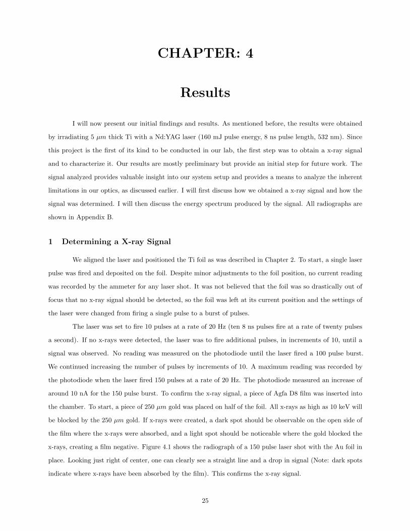
“real,” or best, focus for the OAP actually lies somewhere between the tangential and sagittal foci, as seen in
Figure 3.1 The dilemma is that rays perpendicular to one another have different foci, making alignment and
focal spot determination of the OAP very difficult.
Figure 3.1: Ray diagram showing sagittal, tangential, and best foci
This problem is called an astigmatism and occurs in all OAPs. As mentioned in the previous chapter,
the astigmatism was combated using three HeNe alignment beams but was not fully corrected for. This led
to a few setbacks in alignment, as it was difficult in determining the plane of best focus.
The second spherical aberration that effects the experimentation is coma. Coma is the blurring or
elongation of the focal spot due to light being impingent upon or focused off axis from a mirror or lens. In the
paraxial limit, one can think of the curved surface of the mirror as a bunch of little planar-mirrors connected
together.14 Each planar-mirror will then focus light at a different point, creating an elongated focal spot, as
shown below for a lens.
18

(a) Ray diagram of an off-axis lens creating a coma (b) The coma itself blown up
Figure 3.2: Coma14
Rays close to the principle axis are focused on or near the principle axis, while rays far from the principle
axis are focused far from the other focus. Coming back to the planar-mirror analogy, the rays farther from
the principle axis are hitting mirrors with more severe angles and are being reflected far off the principle axis.
Thus, as one moves farther off-axis, or farther down the line of little planar-mirrors, the coma is increased.
When the outermost rays converge closer to the optical axis than does the principal ray, the image is shrunk
and a negative coma is observed. When the outermost rays converge farther from the optical axis than does
the principal ray, the image is enlarged and a positive coma is observed. Our OAP produces a positive coma
and, so, enlarges the focal spot.
The coma places limits on the size of our focal spot. As seen in the previous figure, a spot is not
actually observed. Instead, a more elongated shape of blotches and arcs is observed. Looking at Figure 3.3,
the coma from our OAP greatly enhances the size of the focal spot. This makes finding the exact focal spot
particularly difficult when its shape is greatly skewed. The center of the spot was taken as the bright point
just below the tip of the coma flare, as a little more than 50% of the energy is found within this tip.14
19

Figure 3.3: Actual picture of focused Nd:YAG spot
As just mentioned, a dramatic consequence of coma is that energy from your beam is spread over a
larger area, reducing your central spot intensity. The coma is a critical flaw in the experimental design that
greatly inhibits x-ray production. Solutions to this problem are outlined in chapter 5.
2 Manufactured Faults in the OAP
Looking at Figure 3.3, what we call the focal spot appears to be stretched into a line shape before
it spreads open into the coma flare. This line is actually the small “spot” scattered along the reflected
meridional plane. Any light reflected off the OAP is scattered because the mirror is not perfectly smooth.
The surface of the mirror is covered in tiny little hills and valleys that reflect light in different directions.
These bumps are a result of the manufacturing process. The mirror is machined from a large piece
of glass down to its final shape and coated with aluminum. It is therefore impossible to achieve a perfectly
smooth surface. Instead, every mirror has a RMS surface roughness measurement that describes the root
mean square vertical distance of the bumps.
20

Figure 3.4: Ray diagram of light scattering off an uneven surface23
Initially worked out by Davies in 1954, Bennett and Porteus developed a theory to describe the
reflectance of a mirror with a slightly rough surface (λ << σ):24,25
RdR0
=
(4πσ cos(θ)
λ
)2
(3.1)
where λ is the wavelength of light, σ is the RMS surface roughness, θ is the angle of incidence, R0 is the
reflectance of a perfectly smooth mirror of the same material, and Rd is the total diffuse reflectance. As
the initial power incident on the mirror is the same for the perfect mirror and rough mirror, it’s easy to see
that the equation above represents the ratio of power lost to scattering effects. Our OAP was quoted by the
manufacturer as having σ < 175 A.26 Taking the upper limit of σ with our 532 nm laser and assuming a 45
degree angle of incidence, the power loss due to scattering comes out to be around 8.5%.
The second factor to consider about the mirror’s make is the metal coating used for its reflective
surface. As light falls on the metal, the light excites lower level electrons in the metal atoms to higher,
excited states. Depending on the atom, the electrons will require different energies to be excited to higher
energy levels. Thus, different metals respond differently to different wavelengths. The electrons absorb the
incident radiation and begin to move around and collide with other atoms, transferring energy and exciting
other electrons. Therefore, some of the energy from the incident light is being absorbed by the mirror and
converted into thermal energy.
Our mirror has an aluminum surface and, according to the manufacturer, has a reflectivity of about
85% at 532 nm.26 Clearly, the laser pulse loses a significant amount of energy through thermal absorption
with the OAP. Combined with the coma and scattering due to surface roughness, the total loss in power for a
laser pulse is roughly 25 - 30%. With this critical loss in energy, it becomes extremely difficult to obtain high
enough intensities to irradiate the foil in only one pulse. The spherical aberrations then place a limit on the
21

location and size of the focal spot one can reliably make out. Regardless of the focal spot we choose, the size
of the spot one can measure is limited by the pixel size of the CCD.
3 CCD Resolution
In regards to this experiment, one needs to consider the sampling of the laser spot on the CCD by
the pixels. Here, there exists a continuous, homogeneous, shape being described by a discrete set of points.
One can see undersampling and oversampling of the spot by the pixels. What this means is that too few
pixels will distort and enlarge the spot, and too many pixels, at a certain point, will add nothing to your
resolution. The heart of this argument lies in the Nyquist Sampling Theorem.
The Nyquist Sampling Theorem describes the translation of information from a continuous signal
into a discrete sequence. Moreover, the Nyquist Sampling Theorem describes the necessary conditions to
successfully sample a continuous sample discretely without loss of information. According to the theorem, a
sampling frequency of at least twice the signal frequency is needed to acquire enough detail to describe the
signal.27 One can easily see this if one thinks of a sine wave. If we sample at twice the frequency of the wave,
then we require all the peaks and troughs of the wave.
A classic example would be that of a strip of movie film. Consider a camera that records a movie with
film. Suppose the camera records the images but at a rate of 2 frames per second. That is, 2 frames are created
on the film strip every 1 second. If one were to watch this movie, any movement that occurred faster than
1/2 s would be lost, and longer movements would appear choppy and blurred. The movie is undersampled
and there is a loss of information. Likewise, a movie filmed at 50 frames per second is oversampled, as the
human eye perceives fluid motions at around 10 - 20 frames per second. An excess of information is obtained
from the sample. Thus, one can find that there is some critical frequency at which all the information can be
collected properly.
(a) Spot centered on a pixel (b) Spot on edges of pixels
Figure 3.5: Spot on pixels of equal size27
If we consider sampling our spot with pixels the size of the spot then we have two scenarios. If the
22

spot is centered on a pixel, then the entire pixel will receive the signal and illuminate, increasing the spot size
a little bit. If the spot lies on the edges of multiple pixels, then all the pixels will be illuminated, increasing
the observed spot again but dimmer. In the above two cases, the size of the spot is increased and the spot is
transformed into a square. The spot has been undersampled and information about the spot’s shape and size
has been lost. Likewise, one can oversample the spot and reduce the field of view. Undersampling can be
seen in Figure 3.5 above.
Ideally, one would want to sample at the critical sampling frequency. It has been found that for
pixelated images, one would like to sample the smallest part of an image with 3.33 pixels.27 For example, if
the smallest part of the image is 300 microns, then one would want the pixels to be around 90 microns. As
shown below, if a spot is made out of three pixels, then one can first start to distinguish the spot’s roundness.
(a) Spot centered on a pixel (b) Spot on edges of pixels
Figure 3.6: Spot on pixels of1
3the size27
Solved in Chapter 2, our laser and OAP produces a theoretical spot size around 10 microns. This would
require 3 micron pixels. No CCD, at least a relatively inexpensive one, has pixels this small. Our CCD has a
pixel size of roughly 8 microns. Thus, our CCD can only correctly resolve an image as small as about 24
microns.
Now, we have found that our measured spot size is directly limited by the CCD. The Nyquist
Sampling Theorem has shown that the smallest resolvable object for our CCD is roughly 24 microns. Looking
back at Eqn. (2.2), the irradiance for this minimally resolvable spot is on the order of 4 ∗ 1012 W/cm2, which
cannot produce the He-alpha like line in Ti.10 Since our measurement of the spot size is limited by the
pixel size of the CCD, the quantitative measurements we can associate with our spot are purely an order of
magnitude estimate and, ultimately, relay little to no information about the real focal spot.
23

4 Conclusion
A key factor in choosing our OAP was the fact that our project was still in its initial design phase
and constrained to a relatively small budget. The ideal, silver coated OAP with smaller surface roughness
would have needed to be custom made and would have cost significantly more. As a result, a cheaper OAP
was purchased as a first test of concept. Only after repeated trial and failure has the flaws of our decision
been observed. At the time of writing, however, lower cost OAP’s have been introduced to the mass market,
and one has been purchased for use. More on this will be discussed in chapter 5.
Spherical aberrations can be greatly reduced with the use of added corrective lenses. Our chamber,
however, lacks the space necessary to place and adjust such corrective lenses. In addition, OAP’s with a
smaller off-axis angle were available to reduce coma. Their focal lengths were often too large or their surface
was coated in a more absorptive metal, such as gold, though.
In concluding this chapter, I would again like to highlight the significance of the OAP to the
experimental setup. As the main focusing optic, the OAP is the main component for achieving x-rays. With
all of the flaws inherent to the current OAP, new, more advanced, focusing optics are being considered that
should reduce aberrations and heighten focal spot intensity.
24
CHAPTER: 4
Results
I will now present our initial findings and results. As mentioned before, the results were obtained
by irradiating 5 µm thick Ti with a Nd:YAG laser (160 mJ pulse energy, 8 ns pulse length, 532 nm). Since
this project is the first of its kind to be conducted in our lab, the first step was to obtain a x-ray signal
and to characterize it. Our results are mostly preliminary but provide an initial step for future work. The
signal analyzed provides valuable insight into our system setup and provides a means to analyze the inherent
limitations in our optics, as discussed earlier. I will first discuss how we obtained a x-ray signal and how the
signal was determined. I will then discuss the energy spectrum produced by the signal. All radiographs are
shown in Appendix B.
1 Determining a X-ray Signal
We aligned the laser and positioned the Ti foil as was described in Chapter 2. To start, a single laser
pulse was fired and deposited on the foil. Despite minor adjustments to the foil position, no current reading
was recorded by the ammeter for any laser shot. It was not believed that the foil was so drastically out of
focus that no x-ray signal should be detected, so the foil was left at its current position and the settings of
the laser were changed from firing a single pulse to a burst of pulses.
The laser was set to fire 10 pulses at a rate of 20 Hz (ten 8 ns pulses fire at a rate of twenty pulses
a second). If no x-rays were detected, the laser was to fire additional pulses, in increments of 10, until a
signal was observed. No reading was measured on the photodiode until the laser fired a 100 pulse burst.
We continued increasing the number of pulses by increments of 10. A maximum reading was recorded by
the photodiode when the laser fired 150 pulses at a rate of 20 Hz. The photodiode measured an increase of
around 10 nA for the 150 pulse burst. To confirm the x-ray signal, a piece of Agfa D8 film was inserted into
the chamber. To start, a piece of 250 µm gold was placed on half of the foil. All x-rays as high as 10 keV will
be blocked by the 250 µm gold. If x-rays were created, a dark spot should be observable on the open side of
the film where the x-rays were absorbed, and a light spot should be noticeable where the gold blocked the
x-rays, creating a film negative. Figure 4.1 shows the radiograph of a 150 pulse laser shot with the Au foil in
place. Looking just right of center, one can clearly see a straight line and a drop in signal (Note: dark spots
indicate where x-rays have been absorbed by the film). This confirms the x-ray signal.
25
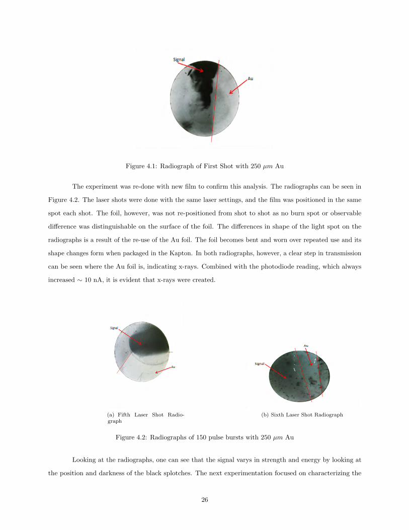
Figure 4.1: Radiograph of First Shot with 250 µm Au
The experiment was re-done with new film to confirm this analysis. The radiographs can be seen in
Figure 4.2. The laser shots were done with the same laser settings, and the film was positioned in the same
spot each shot. The foil, however, was not re-positioned from shot to shot as no burn spot or observable
difference was distinguishable on the surface of the foil. The differences in shape of the light spot on the
radiographs is a result of the re-use of the Au foil. The foil becomes bent and worn over repeated use and its
shape changes form when packaged in the Kapton. In both radiographs, however, a clear step in transmission
can be seen where the Au foil is, indicating x-rays. Combined with the photodiode reading, which always
increased ∼ 10 nA, it is evident that x-rays were created.
(a) Fifth Laser Shot Radio-graph
(b) Sixth Laser Shot Radiograph
Figure 4.2: Radiographs of 150 pulse bursts with 250 µm Au
Looking at the radiographs, one can see that the signal varys in strength and energy by looking at
the position and darkness of the black splotches. The next experimentation focused on characterizing the
26

x-ray signal and determining if the He-alpha like line of Ti was being created.
2 Characterizing the X-ray Signal
The Agfa film was also used to characterize the x-ray signal. A x-ray spectrometer would have been
ideal, but the spectrometer owned by the lab has a temporal resolution on order of a few microseconds. If one
can recall from earlier, the x-rays will be created in a time interval on order of the pulse length, which is 8 ns.
Thus, when the laser fires 150 pulses at a rate of 20 Hz, the majority of the signal will not be recorded by the
spectrometer. Thus, film with different filters was used to determine the x-ray energy based on observable
transmission. This method is much cruder than a spectrometer but still provides a good measure of the
energies produced.
To first test the x-ray signal, stepped pieces of Al were used as filtering on the film. Knowing the
thicknesses and density of the Al, the transmission can yield the opacity of the Al, and the energy of the
x-rays produced can be inferred.4,6 Using the Henke Transmission applet, which utilizes the Beer-Lambert
equation, the transmittance of varying x-ray strengths through the aluminum can be determined. A strip of
Al was folded back half-way and then folded again the opposite way half of the previous fold. This makes a
strip of Al with three thicknesses and can be seen in Figure 4.3.
(a) Stepped Al (SideView)
(b) Film Bundle with Al Steps and Au (FrontFace)
Figure 4.3: Diagrams of Stepped Al and Film Bundle
From top to bottom, the Al goes from one layer thick, to three layers thick, to two layers thick. Therefore,
we should see differences in transmission for the three layers of Al, which should be observable in the film by
differences in darkness. For example, for steps of 10, 20, and 30 µm of Al, the transmission for the He-alpha
energy of Ti should be 50% , 25% , and 10% respectively.15 A shot was done with two pieces of film in place.
27

One piece of film had Al with 10 µm steps in front of it, and the other had Al with 25 µm steps. Both pieces
of film also had the 250 µm Au foil, as well. The two radiographs can be seen below in Figure 4.4, and the
film setup can be seen in Figure 4.3.
(a) Radiograph with 10 µm Al steps (b) Radiograph with 25 µm Al steps
Figure 4.4: Radiographs with Al steps and Au
Looking at the radiographs, it is difficult to determine if the signal on the left is just background or
stepped transmission through the Al. The positions of the Al and Au are lost in the development process, so
one must acertain their positions based on the images produced. This problem is evident in the radiographs
of Figure 4.4. The signal on the left may be background or the transmission through the Al, but it is hard
to determine which because we do not know the position of the Al foil. No definite lines were observed in
transmission, coinciding with the layers of Al, so the signal appears to be background.
To confirm this, another shot was taken with two pieces of film. One piece of film had the 10 µm
stepped Al and no Au foil, while the other piece of film had no filtering and was meant to record only
background. The radiographs are shown below in Figure 4.5.
(a) Radiograph with 10 µm Al steps and noAu
(b) Background Radiograph - Film Only
Figure 4.5: Radiograph with Al steps and Background Radiograph
Comparing the two images, it appears that the film with the Al steps is lighter and has less signal than the
28

background radiograph on the whole. This implies that x-rays are being blocked by the Al. No steps in
transmission are observed on the film with the Al steps either. In fact, there appears to be a distinct line
along the left side of the film, where a strong signal is on the left and a weak signal is on its right. Looking at
the structure and signal on the background radiograph, this straight line is completely unnatural. This can
only come from the Al blocking the x-rays on the right. Combining these observations, one can ascertain that
the x-rays created are not at sufficient energies to penetrate 25 µm of black Kapton and 10 µm of Al. Using
the Henke applet, this corresponds to x-rays that are roughly 2-3 keV.15 Thus, the He-alpha line of Ti is
not being created. Lower energy transitions are being excited in the Al to create these “soft” x-rays, but
the laser is not reaching a high enough irradiance to excite the He-alpha like transition. The laser firing 150
pulses to create x-rays further supports this analysis. Theoretically, a single pulse should work for a perfect
mirror and diffraction-limited focus. As 150 pulses were needed to create x-rays, it is evident that a single
pulse is not even close to the irradiance needed to generate the desired x-rays.
This concludes the characterization. The main goal of this project was to develop an x-ray source
in the lab by irradiating thin metal foils and to obtain the He-alpha like signal from the metals. We found
that the He-alpha like signal was not being produced, so further improvements need to be made to the
experimental setup to obtain a higher irradiance and create the He-alpha like transition in Ti.
29

CHAPTER: 5
Conclusion
Looking back, we have developed an experimental system and method for creating and diagnosing
laser produced x-rays similiar to that of backlighting in HED experiments. A x-ray signal has been detected
and an initial characterization of the signal has been performed. The energy spectrum of the resulting x-rays
has been roughly analyzed, where the He-alpha line of Ti has not been observed. This conclusion informs us
of the inherent faults and errors with our setup. I will conclude this thesis by discussing ideas for future work
and how to improve our current experimental setup to obtain more desireable results. I will leave some final
remarks about the work accomplished and the overarching goal of this project for last.
1 Future Work
Looking back on the work accomplished, there are many improvements that can be made on the
experimental design and procedure. In particular, the OAP, method to measure the focal spot, and laser are
in need of improvement and re-work.
As 150 laser pulses are needed to make low energy x-rays, we can conclude that not enough energy
is being deposited on the foil to irradiate its surface. The main source of error causing this problem is the
OAP. Too much light is being absorbed and scattered, either due to coma or surface roughness, to focus
enough energy to irradiate the foil. At the time of writing, a new OAP, with the same specifications as before,
has been received that has a smaller surface roughness, to reduce scattering, and is silver coated, to reduce
thermal absorption. This OAP should reflect ∼ 14-15% more light to a much tighter focus. The surface
roughness is roughly twice as small, so by Eqn. (3.1), the power loss to scattering should decrease by a factor
of 4. Overall, this new mirror will greatly improve the irradiance achieved by the laser and increase the
chance for creating a He-alpha like signal in a single pulse. In addition, finding the focal spot of the new
OAP should be a little easier because there should be less scattering. The image on the CCD should be more
point-like instead of an elongated line. The coma flare will still exist, however. The coma may be countered
by obtaining an OAP with a less severe off-axis focus.
A more extreme option would be to switch the focusing optic from a mirror to a lens. A OAP
was initially chosen because it offered a higher damage threshold and allowed for an easier setup, given the
chamber dimensions. A lens, however, greatly diminishes the spherical aberrations. The coma would become
30

almost non-existant and the astigmatism would be lessened. Additionaly, aligning the laser beam would
become much simpler because transmitted light would focus on the optical axis of the lens. Unfortunately,
lens’ have a lower damage threshold than OAP’s and take up more system space. A high qulity lens would
cost more than an OAP and require more space in the chamber to allow for focusing along the optical axis.
This would require altering the target holder in the chamber and the chamber itself. The improved OAP will
be tested in our future work, and a lens will be considered if this fails.
Another reason why we may not be reaching the He-alpha like signal with a single pulse is because
we are too far out of focus. The current alignment process involves roughly finding the focal spot by having
the laser fall on a CCD. The pixel resolution of the CCD, however, limits the measurements we can place
on the focal spot. Also, the sizes we are trying to distinguish are too small to easily compare, as shown in
Figure 3.3. That is, when we translate the CCD face a little across the focal plane, the pixel size of the
CCD and the minute physical size of the spot make it difficult to distinguish any noticeable changes in size.
At a certain point, all images produced by the CCD of the beam spot look identical when the CCD face is
traversed along the beam path. This makes determining the exact focus nearly impossible. Even the Python
script cannot accurately determine the size of the focal spot because of its small size, relative to the pixels’,
and background noise from scattered light. To solve this dilemma, magnifying optics, such as a microscope
objective can be used. Placing a microscope objective in front of the CCD would magnify the beam spot and
allow for its size to be determined with greater accuracy. The limited resolution of the CCD by its pixel
size would not be so restrictive, and changes in the micron size spot should become easily visible. The only
foreseeable problem with including a microscope objective in front of the CCD would be the physical space it
would occupy. That is, most objectives are probably too long to be attached to the CCD wthout hitting the
mirror. A microscope objective and camera could be placed off-axis from the foil to image the spot, but this
would require extensive planning and space. A better method for imaging the beam spot should be developed
to ascertain a more accurate measurement of the spot size and to assist in finding the focus. This will lead to
higher irradiances and greater x-ray energies produced.
The last improvement that could be made to increase the likelihood of producing x-rays with a single
energy pulse is to get a laser with a higher pulse energy or shorter pulse length. A more intense laser would
simply deposit more energy on the foil, creating higher energy electrons to initiate higher energy transitions.
For example, a 1 J laser would increase the focal intensity by a full order of magnitude. This suggestion
is to be taken more in thought than in practice, however. A more intense laser would require upgrading
a considerable amount of optics to higher damage thresholds, and the price for a new laser is not within
the budget. Simply put, a more intense laser would greatly help with this project but is not of practical
consideration at the moment.
31

As we are not obtaining sufficient energies to create the He-alpha like line for Ti, one could then try
to irradiate a metal with a lower He-alpha like line, like Al. The He-alpha like line for Al, however, is too
low. The black Kapton filtering would block almost all of the created signal, and 25 µm black Kapton is the
thinnest that can be purchased easily. As for other metals between Al and Ti, there simply aren’t that many
of particular interest to be used in backlighting experiments. Thus, increasing the intensity to irradiate Ti is
the only path to take.
2 Concluding Remarks
The overall merit and work of this project has been a great accomplishment for the lab. This project
was first proposed as a test of concept to the see if x-ray backlighting could be replicated in the lab with
a common table-top laser. Based on a limited budget and an assortment of equipment around the lab, an
experimental apparatus and procedure was developed that produced x-rays. The signal produced, however,
did not have the He-alpha like emission that is characteristic of low-irradiance backlighting. Nevertheless,
a conclusion has been drawn from our experimentation that has indeed given a proof of concept. With
further development of the experiment, it is believed that higher irradiances can be achieved and that x-ray
backlighting can be replicated in the lab setting, as desired.
32

Appendix A
A.1
Python code for finding spot size on CCD.
#functions/libraries
from __future__ import division#, print_function
from pylab import imshow,show,jet,hot,xlabel,ylabel,title,plot,xticks,yticks,axhline
import matplotlib.image as mpimg
import numpy as np
from PIL import Image
import os
#pixel dimensions of CCD
pixSizeV=9.8*(10/31.497976) #in microns; scaled to new image size from ccd
pixSizeH=8.4*(10/31.497976) #in microns; scaled to new image size from ccd
filename=raw_input("Input file name as .png: ")
#checks for existence of file
check=os.path.isfile(filename)
while(check != True):
print("Invalid file name. Try again.")
filename=raw_input("Input file name as .png: ")
check=os.access(filename,os.F_OK)
#open Image
img=Image.open(filename)
#version of Image from which size can be read
img2=mpimg.imread(filename)
img3=img.convert("L") #L = R * 299/1000 + G * 587/1000 + B * 114/1000
#Effectively, allows for use in imshow
#directions
print(’’)
print("For the following contrast map, take note of the x value about which the")
print("spot appears to be centered. Close graph when done.")
raw_input("Press ENTER to continue")
#contrast map
tsx=np.arange(0,img2.shape[1],(img2.shape[1]/10))
tvx=np.arange(0,1,.1)
tsy=np.arange(0,img2.shape[0],(img2.shape[0]/10))
tvy=np.arange(0,1,.1)
imshow(img3, origin="lower")
xticks(tsx,tvx)
33

yticks(tsy,tvy)
hot()#jet() #makes contrast map
title("Contour Map of Beam Spot")
xlabel("x-position")
ylabel("y-position")
show()
#get line out from center of spot
pixdata=[]
print(’’)
N=raw_input("How far to the right is the center of the spot?(give as decimal between 0-1):")
n=float(N)
for y in range(0, img2.shape[0]):
red,green,blue=img.getpixel((y,n*img2.shape[0]))#(n*img2.shape[0],y))
pixdata.append(0.299*red+0.587*green+0.114*blue)
#95%, 5%, and half way between values
top=max(pixdata)*.95
bottom=max(pixdata)*.05
HalfMax=(top+bottom)/2
#Fast Fourier Transform
#"smooth" data out
c=np.fft.rfft(pixdata)
length=len(c)
for i in range(length):
if i>.02*(length):
c[i]=0
cnew=np.fft.irfft(c)
#directions for user
print(’’)
print("For follwing plot, move cursor over intersection of HalfMax (red)")
print("and line out (blue) and note x-position on bottom of graph.")
print("Round to nearest integer, this is your pixel value.")
print("Do this for both intersections and note pixel values.")
print("Close graphs when done.")
raw_input("Press ENTER to continue ")
print(’’)
#plot line out and HalfMax
plot(pixdata) #actual data
plot(cnew,"g") #"smooth version"
xlabel("Pixel Number")
ylabel("Weighted Pixel Count")
title("Line Out of Mid-Image")
axhline(HalfMax,0,len(pixdata),color=’r’)
show()
#initialize outside for scope
rightPt=0
leftPt=0
34

#user input for left pt
check2=True
while(check2):
leftPt=raw_input("Enter left pixel number for Half-Max as int: ")
if (leftPt.isdigit()):
check2=False
else:
print("Input is not an integer or negative. Try again.")
#user input for right pt
check3=True
while(check3):
rightPt=raw_input("Enter right pixel number for Half-Max as int: ")
if (rightPt.isdigit() and rightPt > leftPt):
check3=False
else:
if (rightPt.isdigit() == False):
print("Input is not an integer or negative. Try again.")
elif (rightPt <= leftPt):
print("Input not greater than left point. Try again.")
#print values
print(’’)
print("5% of Max is:",bottom)
print("95% of Max is:",top)
print("FWHM is:",(int(rightPt)-int(leftPt))*pixSizeV,"microns")
#new axes for contrast map, in microns
tickSpotsx=np.arange(0,img2.shape[1],(img2.shape[1]/7))
tickValsx=np.arange(0,img2.shape[1]*pixSizeH,round(img2.shape[1]*pixSizeH/7,2))
tickSpotsy=np.arange(0,img2.shape[0],(img2.shape[0]/5))
tickValsy=np.arange(0,img2.shape[0]*pixSizeV,round(img2.shape[0]*pixSizeV/5,2))
#contrast map
imshow(img3, origin="lower")
xticks(tickSpotsx,tickValsx)
yticks(tickSpotsy,tickValsy)
jet() #makes contrast map
title("Contour Map of Beam Spot")
xlabel("x-position (microns)")
ylabel("y-position (microns)")
show()
35

A.2
Beam Profile for Alignment Laser
36

Appendix B
Radiograph of First Shot with 250 µm Au
Radiograph of Second Shot with 250 µm Au
Radiograph of Third Shot with 250 µm Au
37

Radiograph of Fourth Shot with 250 µm Au
Radiograph of Fifth Shot with 250 µm Au
Radiograph of Sixth Shot with 250 µm Au
38

Radiograph of Seventh Shot with 250 µm Au
Radiograph of Eighth Shot with 250 µm Au and 10 µm Al Steps
Radiograph of Eighth Shot with 250 µm Au and 25 µm Al Steps
39

Radiograph of Ninth Shot with 25 µm Al Steps
Background Radiograph of Ninth Shot
Radiograph of Tenth Shot with 10 µm Al Steps
40

Background Radiograph of Tenth Shot
Background Radiograph of Tenth Shot with New Film Bundle Style
41

References
1 Drake, R. P. High-Energy-Density Physics: Fundamentals, Inertial Fusion, and Experimental Astrophysics.Springer. (2006).
2 R. P. Drake,. Physics Today. “High-energy-density physics”. (June 2010).
3 R. C. Davidson et al. Frontiers in High Energy Density Physics: The X-games of Contemporary Science.National Academies Press. Washington, DC. (2003).
4 Kuranz, Carolyn. Blast-wave-driven, multidimensional Rayleigh-Taylor instability experiments. University ofMichigan. (2009).
5 C. C. Kuranz, B. E. Blue, R. P. Drake, H. F. Robey, J. P. Knauer et al. Rev. Sci. Instrum. 77. 10E327(2006).
6 Doss, Forrest. Structure in Radiative Shock Experiments. University of Michigan. (2011).
7 Huntington, Channing. High-Energy-Density Physics Experiments Relevant to Astrophysical Systems. Uni-versity of Michigan. (2012).
8 C. M. Krauland, L. C. Jarrott, R. P. Drake, P. A. Keiter, C. C. Kuranz et al. Rev. Sci. Instrum. 83. 10E528(2012).
9 H. S. Park, D. M. Chambers, H. K. Chung, R. J. Clarke, R. Eagleton et al. Physics of Plasmas. 13. 056309(2006).
10 J. Workman, N. E. Lanier, and G. A. Kyrala. American Institute of Physics. 74. 3 (2002).
11 McCrory, Robert. University of Rochester - Laboratory for Laser Energetics. <www.rochester.lle.edu>.(2013).
12 Baisden, Trish, Bonnano, Regina, & Reyes, Susana. Lawrence Livermore National Laboratories - NationalIgnition Facility. <lasers.llnl.gov>. (2013).
13 Heald, Mark & Marion, Jerry. Classical Electromagnetic Radiation. 4th Ed. Saunders College Pub. FortWorth. (1995).
14 Hecht, Eugene. Optics. 4th Ed. Pearson Education Inc. San Francisco. (2002).
15 B.L. Henke, E.M. Gullikson, and J.C. Davis. X-ray interactions: photoabsorption, scattering, transmission,and reflection at E=50-30000 eV, Z=1-92, Atomic Data and Nuclear Data Tables. 54, 181-342 (1993).
16 D. Bradley, O. Landen, A. Bullock, S. Glendenning, & R. Turner. Optics Letters. 37. (2002).
17 Eliezer, Shalom & Mima, Kunioki. Applications of Laser-Plasma Interactions. Taylor & Francis Group.Boca Raton. (2009).
18 G. A. Kyrala. Rev. Sci. Instrum. 77. 055104 (2006).
19 Pinhole Camera. <en.wikipedia.otg/wiki/Pinhole camera>. (2013).
20 Off-axis Parabolic Metal Mirrors. <thorlabs.com>. (2013).
21 AXUV Series - Absolute UV Silicon Photodiodes. <www.optodiode.com/library.html>. (2013).
22 N. E. Lanier, J. S. Cowan, and J. Workman. Rev. Sci. Instrum. 77. 043504 (2006).
23 Diffuse Reflection. <www.sciencelearning.org/Contexts/Light-and-Sight/Images/Types-of-Reflection>.(2012).
24 H. Davies. Proc. Inst. Elec. Eng. 101. 209 (1954).
42

25 H. E. Bennett, J. O. Porteus. JOSA. 51. 2 (1961).
26 Off-Axis Parabolic Metal Mirrors. <www.edmundoptics.com>. (2013).
27 Nyquist Theorem. <starizona.com/abc/ccd/advtheorynyq.aspx>. (2013).
43