Embed Size (px)
Citation preview

Control of sound transmission into payload fairings using distributed vibration absorbers
and Helmholtz resonators.
Simon J. Estève
Dissertation submitted to the Faculty of the Virginia Polytechnic Institute and State University in partial fulfillment of the
requirements for the degree of
Doctor of Philosophy In
Mechanical Engineering
Dr. Martin E. Johnson, Chairman Dr. Ricardo A. Burdisso
Dr. Robert L. Clark Dr. Christopher R. Fuller
Dr. Donald J. Leo
May 6th 2004
Blacksburg, Virginia
Keyword: Acoustic transmission, Helmholtz resonator, vibration absorber, payload fairing.
2004 by Simon J. Estève

Control of sound transmission into payload fairings using distributed vibration absorbers
and Helmholtz resonators.
Simon J. Estève
Abstract
A new passive treatment to reduce sound transmission into payload fairing at low
frequency is investigated. This new solution is composed of optimally damped vibration
absorbers (DVA) and optimally damped Helmholtz resonators (HR). A fully coupled
structural-acoustic model of a composite cylinder excited by an external plane wave is
developed as a first approximation of the system. A modal expansion method is used to
describe the behavior of the cylindrical shell and the acoustic cavity; the noise reduction
devices are modeled as surface impedances. All the elements are then fully coupled using
an impedance matching method. This model is then refined using the digitized mode
shapes and natural frequencies obtained from a fairing finite element model.
For both models, the noise transmission mechanisms are highlighted and the noise
reduction mechanisms are explained. Procedures to design the structural and acoustic
absorbers based on single degree of freedom system are modified for the multi-mode
framework. The optimization of the overall treatment parameters namely location, tuning
frequency, and damping of each device is also investigated using genetic algorithm.
Noise reduction of up to 9dB from 50Hz to 160Hz using 4% of the cylinder mass for the
DVA and 5% of the cavity volume for the HR can be achieved. The robustness of the
treatment performance to changes in the excitation, system and devices characteristics is
also addressed.

iii
The model is validated by experiments done outdoors on a 10-foot long, 8-foot
diameter composite cylinder. The excitation level reached 136dB at the cylinder surface
comparable to real launch acoustic environment. With HRs representing 2% of the
cylinder volume, the noise transmission from 50Hz to160Hz is reduced by 3dB and the
addition of DVAs representing 6.5% of the cylinder mass enhances this performance to
4.3dB. Using the fairing model, a HR+DVA treatment is designed under flight
constraints and is implemented in a real Boeing fairing. The treatment is composed of
220 HRs and 60 DVAs representing 1.1% and 2.5% of the fairing volume and mass
respectively. Noise reduction of 3.2dB from 30Hz to 90Hz is obtained experimentally.
As a natural extension, a new type of adaptive Helmholtz resonator is developed. A
tuning law commonly used to track single frequency disturbance is newly applied to track
modes driven by broadband excitation. This tuning law only requires information local to
the resonator simplifying greatly its implementation in a fairing where it can adapt to
shifts in acoustic natural frequencies caused by varying payload fills. A time domain
model of adaptive resonators coupled to a cylinder is developed. Simulations demonstrate
that multiple adaptive HRs lead to broadband noise reductions similar to the ones
obtained with genetic optimization. Experiments conducted on the cylinder confirmed the
ability of adaptive HRs to converge to a near optimal solution in a frequency band
including multiple resonances.

iv
Acknowledgements
I would like to thank my research advisor, Professor Marty Johnson, for giving me
the opportunity to be involved in a challenging research project, and most of all for
making these past four years such an enjoyable and rewarding experience. Indeed, with
his great personality, he is an outstanding advisor who always listens respectfully and
imparts his knowledge so willingly.
I would also like to thank the members of my committee, Professor Ricardo Burdisso,
Professor Chris Fuller, and Professor Donald Leo, for the quality education and advice
they provided, and also Professor Robert Clark for accepting to serve on my committee
despite the distance.
I am obviously indebted to the Boeing Company for supporting this work and wish to
thank in particular Haisam Osman for his interest in this research, but more so for his
kindness.
Many thanks go to the people at VAL, James Carneal for his helpful support, Michael
Kidner for his scientific and English writing advice, and my fellow students Michael
James, Tony Harris and Ozer Sarcacelik for their help and friendship during the course of
this work.
My parents, my brother and my sister in France, who have always been and will ever
be simply wonderful, deserve all my gratitude for their unconditional support and
encouragement during the pursuit of my education in the United States despite the
physical and cultural distance.
Finally, I would like to thank my future wife, Michelle, and her parents, Judy and
Don, for making Virginia my second home and for the love they are surrounding me
with.

v
Table of Content
Abstract ...............................................................................................ii
Acknowledgements ............................................................................iv
Table of Content ................................................................................. v
List of Figures.....................................................................................ix
List of Tables ....................................................................................xiv
List of Pictures...................................................................................xv
Chapter 1 Introduction ................................................................... 1
1.1 Motivation and existing solutions....................................................1
1.2 Research development on the payload fairing noise problem......3 1.2.1 Active control approach .......................................................................3 1.2.2 Passive treatment................................................................................5
1.3 The dynamic vibration absorber ......................................................7 1.3.1 How it works ........................................................................................7 1.3.2 A well-studied system........................................................................10 1.3.3 The Distibuted Vibration Absorber (DVA) ..........................................12
1.4 The Helmholtz resonator ................................................................14 1.4.1 Principle and modeling ......................................................................14 1.4.2 Applications .......................................................................................17 1.4.3 Adaptive Helmholtz Resonator (AHR) ...............................................19
1.5 Objectives of this research.............................................................20
1.6 Contribution of the work.................................................................22
Chapter 2 Modeling ..................................................................... 24
2.1 Introduction .....................................................................................24

vi
2.2 Composite cylinder vibration analysis ..........................................25 2.2.1 Equation of motion.............................................................................25 2.2.2 Boundary conditions, mode shapes and natural frequencies ............30 2.2.3 Forced vibrations ...............................................................................34 2.2.4 External Fluid loading effect ..............................................................38
2.3 Acoustic cavity analysis .................................................................47 2.3.1 Mode shapes and natural frequency of an acoustic cavity ................47 2.3.2 Forced response of an acoustic cavity ..............................................51
2.4 Structural-acoustic spatial coupling..............................................53 2.4.1 External spatial coupling....................................................................53 2.4.2 Internal spatial coupling.....................................................................57
2.5 Implementation of the noise reduction devices............................59 2.5.1 Modeling............................................................................................59 2.5.2 Spatial coupling .................................................................................60
2.6 Fully coupled system response .....................................................62
2.7 Model using finite element outputs ...............................................65 2.7.1 Conversion of the components in discrete form ................................66 2.7.2 External excitation numerical model ..................................................66
2.8 Conclusions.....................................................................................70
Chapter 3 Numerical simulations................................................. 71
3.1 Introduction .....................................................................................71
3.2 Noise transmission mechanisms...................................................71 3.2.1. External coupling ...............................................................................72 3.2.2. Internal coupling ................................................................................76 3.2.3. Fluid loading effect ............................................................................81 3.2.4. Model validation ................................................................................84 3.2.5. Fairing model.....................................................................................97
3.3 Noise reduction mechanisms.......................................................105 3.3.1. Optimal damping .............................................................................105 3.3.2. Devices are used in rings. ...............................................................109 3.3.3. Influence of the DVA mass and HR volume. ...................................110 3.3.4. Experimental validation. ..................................................................111
3.4 Treatment design for the Boeing cylinder...................................117 3.4.1 Targeting individual modes: the “manual” treatment design ............117 3.4.2 Treatment design using a genetic algorithm....................................122
vii
3.4.3 Performance robustness to uncertainty in the excitation, system and treatment .........................................................................................130
3.4.4 Performance of random treatments .................................................131
3.5 Treatment design for the payload fairing ....................................132 3.5.1 The “manual” solution......................................................................132 3.5.2 Genetic algorithm solution ...............................................................135 3.5.3 Performance robustness to variation in the excitation, system and
treatment. ........................................................................................138 3.5.4 Performance of random treatments .................................................140
3.6 Conclusions...................................................................................140
Chapter 4 Outdoor high level tests ............................................ 144
4.1 Introduction ...................................................................................144
4.2 Empty cylinder test November 14th-30th, 2001 ............................144 4.2.1. Test setup........................................................................................145 4.2.2. Noise reduction treatment ...............................................................148 4.2.3. Results ............................................................................................150
4.3 Partially filled cylinder test October 2002 ...................................159 4.3.1 Test setup........................................................................................159 4.3.2 Noise reduction treatment ...............................................................161 4.3.3 Results ............................................................................................167
4.4 Fairing test November-December 2003 .......................................172 4.4.1 Lightweight Helmholtz resonator design..........................................172 4.4.2 Noise reduction treatment design....................................................177 4.4.3 Experimental setup..........................................................................181 4.4.4 Results. ...........................................................................................183
4.5 Conclusions...................................................................................187
Chapter 5 Adaptive Helmholtz resonator................................... 189
5.1 Introduction ...................................................................................189
5.2 Time domain model.......................................................................189 5.2.1 Governing equations .......................................................................190 5.2.2 Matrix formulation of the system......................................................193
5.3 Tuning algorithm ...........................................................................196 5.3.1 Local strategy for global control.......................................................196 5.3.2 The dot-product method ..................................................................199

viii
5.4 Numerical simulations ..................................................................202 5.4.1 Single mode forced by an internal source .......................................203 5.4.2 Multi-mode forced by an external plane wave .................................204
5.5 Experimental results .....................................................................207 5.5.1 Adaptive Helmholtz resonator prototype..........................................207 5.5.2 Control system.................................................................................211 5.5.3 Experimental set-up.........................................................................212 5.5.4 Results ............................................................................................214
5.6 Conclusions...................................................................................220
Chapter 6 Conclusions and future work..................................... 222
6.1 Conclusions...................................................................................222
6.2 Future work....................................................................................225
Appendix A Acoustic damping scaling ......................................... 227
Bibliography.................................................................................... 231
Vita ................................................................................................. 240

ix
List of Figures
Figure 1.1 Contour of equal overall SPL (Eldred 1971)..................................................... 3 Figure 1.2 Model of a dynamic vibration absorber attached to a host structure................. 9 Figure 1.3 Distributed Vibration Absorber....................................................................... 14 Figure 1.4 (a) Sketch of a HR exposed to an external acoustic pressure p and through
whose neck flows a volume velocity u. (b) mechanical analog............................ 16 Figure 2.1 Schematic of the analytical cylinder model and the finite element based fairing
............................................................................................................................... 25 Figure 2.2 Schematic of the sandwich cylinder. ............................................................... 27 Figure 2.3 Natural frequencies of the cylinder for n=1. ................................................... 34 Figure 2.4 Normalized radiation impedance of an infinite cylinder for m=0,1,2,3 and
kz=1. ...................................................................................................................... 43 Figure 2.5 Cylinder mounted in an infinite baffle and excited by an acoustic plane wave.
............................................................................................................................... 57 Figure 2.6 Coupling between the cylinder and the noise reduction devices: HRs and
DVAs .................................................................................................................... 61 Figure 2.7 Block diagram of the fully coupled system..................................................... 65 Figure 2.8 Location of evaluation points, equivalent sources and primary source used to
model an outdoor acoustic excitation. .................................................................. 69 Figure 3.1 Magnitude of
s smP σ due to an incident plane wave of 1Pa. (αi=70°,θi=0°) and frequency as a function of the normalized horizontal wave number in air krR for ms=0,1,2,3. ............................................................................................................ 73
Figure 3.2 Magnitude of the axial mode shape’s wavenumber transform and frequency as a function of the normalized axial wave number in air for ns=1,2,3,4. ................ 74
Figure 3.3 In vacuo response of the cylinder structural kinetic energy as function of frequency due a plane wave excitation of elevation angle α and due to a point force excitation...................................................................................................... 75
Figure 3.4 Dispersion curves for the Boeing cylinder in ‘n’ groups and for the equivalent infinite sandwich plate without core shear............................................................ 77
Figure 3.5 Contours of the structural and acoustic resonant frequencies as a function of their mode orders. ................................................................................................. 79
Figure 3.6 Structural kinetic energy and acoustic potential energy of an empty cylinder excited by an oblique plane wave (αi=70°). ......................................................... 80
Figure 3.7 Structural kinetic energy and acoustic potential energy of an annular cylinder excited by an oblique plane wave (αi=70°). ......................................................... 80
Figure 3.8 Real and imaginary part of the normalized radiation impedance as function of frequency for three different modes with scaled modal response (dotted line). ... 83
Figure 3.9 Influence of the external fluid loading on the structural kinetic energy and the acoustic potential energy of the cylinder under oblique plane wave excitation (αi=70°)................................................................................................................. 83

x
Figure 3.10 Boeing composite cylinder on its dolly with the 5 rings of 30 accelerometers................................................................................................................................ 84
Figure 3.11 Picture and schematic of the volume velocity speaker with internal microphone. .......................................................................................................... 85
Figure 3.12 Experimental and predicted acoustic response at two microphones locations............................................................................................................................... 86
Figure 3.13 Experimental and predicted spatially averaged SPL (15 microphones) per volume velocity (VV). .......................................................................................... 87
Figure 3.14 Mode amplitudes extracted from the microphone data and predicted by the numerical code. ..................................................................................................... 89
Figure 3.15 Experimental and predicted velocity response per unit force at the excitation location and at position 65 (3rd ring up)................................................................ 92
Figure 3.16 Experimental and predicted mean velocity squared per unit force (151 positions)............................................................................................................... 93
Figure 3.17 Experimental and predicted modal amplitudes. ............................................ 94 Figure 3.18 Symmetric component of the normalized velocity wavenumber transform
applied on the lower ring using the predicted (top) and measured (bottom) response................................................................................................................. 95
Figure 3.19 Measured and predicted internal SPL per unit input force using the theoretical coupling matrix (top) and the “noisy” coupling matrix (bottom). ...... 97
Figure 3.20 Fairing structural mode shapes with the corresponding cylindrical section mode order. ........................................................................................................... 98
Figure 3.21 Circumferential wavenumber transform of the fairing velocity response to a point force. ............................................................................................................ 99
Figure 3.22 External pressure distribution on the fairing due to eight speakers at 70Hz.............................................................................................................................. 100
Figure 3.23 Acoustic damping ratio obtained from 1/3 octave T60 measurement. ......... 102 Figure 3.24 Overall coupling level between structural acoustic modes. ........................ 104 Figure 3.25 Velocity and acoustic response to speaker excitation using the complete
modal set and the modal subset. ......................................................................... 105 Figure 3.26 Optimal damping ratios using Eq.(3.3.1) and Eq.(3.3.3) as a function of
effective mass and volume ratios........................................................................ 107 Figure 3.27 Influence of the DVA and HR damping ratios on the kinetic and acoustic
energy.................................................................................................................. 108 Figure 3.28 Influence of the number of DVA per ring on the amplitude of the 1,2 and 1,6
structural mode.................................................................................................... 110 Figure 3.29 Influence of the DVA mass and HR volume in percent of the total mass and
total volume of the cylinder on the kinetic and acoustic energy......................... 111 Figure 3.30 Example of a 3”x5” DVA made with 2” thick polyurethane foam............. 112 Figure 3.31 Experimental set-up used to tune DVA....................................................... 112 Figure 3.32 Measured and predicted vibration response of the bare (dotted line) and the
DVAs treated cylinder (solid)............................................................................. 113 Figure 3.33 Measured and predicted acoustic response of the bare (dotted line) and the
DVAs treated cylinder (solid)............................................................................. 114 Figure 3.34 Damped Helmholtz resonator made from cardboard tube and foam screen.
............................................................................................................................. 115

xi
Figure 3.35 Experimental set-up used to tune HR.......................................................... 115 Figure 3.36 Measured (left) and predicted (right) normalized acoustic response under
external acoustic excitation with and without the HR treatment. ....................... 116 Figure 3.37 Acoustic and kinetic energy of the bare cylinder including acoustic re-
radiation. ............................................................................................................. 118 Figure 3.38 Narrow and third octave acoustic energy reduction for the “manual”
treatment design. ................................................................................................. 119 Figure 3.39 Narrow and third octave band kinetic energy reduction for the “manual”
treatment design. ................................................................................................. 120 Figure 3.40 Acoustic attenuation as a function of the initial acoustic & structural damping
ratio for the treatment in Table 3.5 with adjusted optimal damping ratios......... 121 Figure 3.41 Convergence of the genetic algorithm for run#1 and 2. .............................. 124 Figure 3.42 Narrow and third octave acoustic energy reduction for a genetically
optimized treatment. ........................................................................................... 125 Figure 3.43 Narrow and third octave band vibration attenuation for the genetically
optimized treatment. ........................................................................................... 126 Figure 3.44 Convergence of the genetic algorithm for run#3......................................... 127 Figure 3.45 Convergence of the genetic algorithm for run#3......................................... 128 Figure 3.46 Position of the DVA and HR tuning frequencies around the cylinder
circumference for the genetic solution of run#4. ................................................ 129 Figure 3.47 Noise attenuation of the run#4 treatment as a function of the azimuth angle θi
of the incident wave. ........................................................................................... 129 Figure 3.48 Robustness of the treatment with respect to the elevation angle of the incident
plane wave. ......................................................................................................... 131 Figure 3.49 Narrow and third octave fairing internal SPL reduction for the “manual”
treatment design. ................................................................................................. 134 Figure 3.50 Narrow and third octave fairing vibration reduction for the “manual”
treatment design. ................................................................................................. 134 Figure 3.51 Convergence of the genetic algorithm......................................................... 136 Figure 3.52 Narrow and third octave fairing internal SPL reduction for the genetically
optimized treatment. ........................................................................................... 137 Figure 3.53 Narrow and third octave fairing vibration reduction for the genetically
optimized treatment. ........................................................................................... 137 Figure 3.54 Fairing top and side view for different disturbance speaker configurations
and the resulting attenuation obtained with genetic solution.............................. 139 Figure 4.1 Schematic showing the positions of all of the measurement equipment....... 147 Figure 4.2 DVAs spaced every 240 and around the midpoint up the cylinder................ 149 Figure 4.3 Structural modal components of the external acoustic field at 4 different
frequencies. ......................................................................................................... 151 Figure 4.4 Variation of the external pressure distribution along the length of the cylinder
as a function of frequency................................................................................... 152 Figure 4.5 Narrow and third octave band external SPL for the three different
configurations. .................................................................................................... 153 Figure 4.6 Normalized velocity wavenumber transform applied on the ring of
accelerometers..................................................................................................... 154
xii
Figure 4.7 Narrow and third octave band vibration performance of the DVA and DVA+HR treatment compare to the bare baseline. ............................................ 155
Figure 4.8 Narrow and third octave band acoustic performance of the HR and HR+DVA treatments compare to the bare baseline. ............................................................ 156
Figure 4.9 Narrow and third octave band vibration performance of the HR and HR+DVA treatments compare to the half foam baseline..................................................... 157
Figure 4.10 Narrow and third octave band acoustic performance of the HR and HR+DVA treatments compare to the half foam baseline..................................................... 158
Figure 4.11: Cylinder inside the tent and experiment layout diagram............................ 159 Figure 4.12 Acoustic mode shape of the partially filled cavity obtained from Boeing finite
element model..................................................................................................... 162 Figure 4.13 Low-level acoustic transmission with payload set up. ................................ 162 Figure 4.14: mean square pressure transfer functions (64 microphones) ....................... 163 Figure 4.15 HR/DVA and its bouncing natural frequency curve. .................................. 166 Figure 4.16 Characteristics of the external acoustic field created on the cylinder by one
side of speaker..................................................................................................... 168 Figure 4.17 Narrow and third octave external SPL averaged between mic#1 and mic#3.
............................................................................................................................. 169 Figure 4.18 Narrow and third octave band vibration performance of the HR and
combined HR+DVA treatment compared to the half foam baseline.................. 170 Figure 4.19 Narrow and third octave band acoustic performance of the HR and HR+DVA
treatments compared to the half foam baseline................................................... 171 Figure 4.20 Transfer function between internal and external pressure obtained with the
cardboard and PETG HR. ................................................................................... 174 Figure 4.21 Transfer function of a PETG HR with and without stiffener. ..................... 176 Figure 4.22 Speaker layout for the payload fairing test.................................................. 178 Figure 4.23 HR and DVA layout in the fairing blanket.................................................. 179 Figure 4.24 Prediction of the acoustic performance of the treatment tested in the fairing.
............................................................................................................................. 181 Figure 4.25 Location of the accelerometers and microphones for the fairing test. ........ 183 Figure 4.26 Narrow and third octave band level of the average external SPL for both
tests. .................................................................................................................... 184 Figure 4.27 Circumferential wavenumber transform of the velocity response of the upper
ring for both treatments....................................................................................... 185 Figure 4.28 Narrow and third octave vibration performance of the fairing treatment. .. 186 Figure 4.29 Acoustic performance prediction with lowered acoustic natural frequencies.
............................................................................................................................. 187 Figure 5.1 Schematic of the different local cost functions for a tunable vibration absorber.
............................................................................................................................. 197 Figure 5.2 Cost functions as a function of absorber tuning frequency using13 modes. . 198 Figure 5.3 Cross-spectrum of and under tuned HR (left) and tuned HR right with respect
to a single resonance at 100Hz............................................................................ 201 Figure 5.4 Change in the dot-product and tuning frequency of the 3 HRs as a function of
time. .................................................................................................................... 204 Figure 5.5 Structural kinetic (Ek) and acoustic potential (Ep) energy with and without
DVA treatment (one-way coupled model).......................................................... 205
xiii
Figure 5.6 Acoustic potential energy before and after adaptation compared to the bare case...................................................................................................................... 206
Figure 5.7 Adaptive Helmholtz resonator prototype. ..................................................... 208 Figure 5.8 Motorized iris diaphragm mechanism. .......................................................... 208 Figure 5.9 Measured natural frequency and damping ratio without screen for different
opening diameters. .............................................................................................. 210 Figure 5.10 Iris diaphragm with wire mesh screen for constant damping...................... 210 Figure 5.11 Measured natural frequency and damping ratio with screen for different
opening diameters. .............................................................................................. 211 Figure 5.12 Control system for 8 resonators................................................................... 212 Figure 5.13 Top view of the inside of the cylinder......................................................... 213 Figure 5.14 Evolution of the opening diameter for the 8 HRs........................................ 215 Figure 5.15 Magnitude and phase of the transfer function of HRs #2 and #8................ 216 Figure 5.16 Normalized cross-spectrum of HR#4 and HR#6......................................... 216 Figure 5.17 Acoustic response of the cavity before and after the adaptation ................. 217 Figure 5.18 Evolution of the opening diameter for the 8 HRs........................................ 218 Figure 5.19 Normalized cross-spectrum of HR#2 and #4 .............................................. 219 Figure 5.20 Acoustic response before and after adaptation............................................ 220 Figure A.1 Mean square pressure response to the source shut-off for the payload fairing.
............................................................................................................................. 227 Figure A.2 100 Hz third octave band decaying signal for the payload fairing............... 228 Figure A.3 Mean square pressure response to the source shut-off for the bare cylinder.229

xiv
List of Tables
Table 2.1 Physical dimensions and material characteristics of the Boeing cylinder. ....... 26 Table 2.2 Illustration of the diagonal dominance of the radiation impedance matrix ...... 46 Table 3.1 Structural resonant frequency of the Boeing cylinder below 200Hz................ 76 Table 3.2 Additional damping ratio, and mass ratio for the Boeing cylinder modes due to
the fluid loading effect. ......................................................................................... 82 Table 3.3 List of measured, theoretical and fully coupled acoustic natural frequencies. . 89 Table 3.4 Examples of additional damping ratio, and mass ratio for fairing modes due to
the fluid loading effect. ....................................................................................... 101 Table 3.5 Parameters of the “manual” treatment design................................................. 119 Table 3.6 Acoustic attenuation in the 50-160 Hz band obtained with the treatment in
Table 3.5 for different total mass of DVAs and total volume of HRs with optimal damping ratios computed accordingly. ............................................................... 122
Table 3.7 Parameters of the genetically optimized treatment for run#1 (in blue) and run#2 in red. .................................................................................................................. 124
Table 3.8 Performance comparison between the “manual” treatment in Table 3.5 and the genetic algorithm solution for different mass of DVAs and volume of HRs. .... 126
Table 3.9 Parameters of the genetically optimized treatment for run#3......................... 127 Table 3.10 Parameters of the “manual” treatment design............................................... 133 Table 3.11 Parameters of the genetically optimized treatment....................................... 136 Table 3.12 Performance robustness to changes in the system and treatment
characteristics...................................................................................................... 140 Table 4.1 Description of the Helmholtz resonator treatment.......................................... 148 Table 4.2 Resonant frequencies of the cavity filled with the mock payload .................. 164 Table 4.3 Description of the Helmholtz resonator treatment.......................................... 164 Table 4.4 HR parameters of the launch vehicle treatment.............................................. 180 Table 4.5 DVA parameters of the launch vehicle treatment........................................... 180 Table 5.1 Tuning frequency of the 8 HR before and after the single mode adaptation.. 215 Table 5.2 Tuning frequency of the 8 HRs before and after the multi mode adaptation. 219 Table A.1 Comparison of the third octave band reverberation time............................... 230

xv
List of Pictures
Picture 4.1 Cylinder being craned onto the base and then placed under the large tent at the outdoor test site. .................................................................................................. 145
Picture 4.2 Test site showing the tent, equipment trailer and the power generator ........ 146 Picture 4.3 Instrumented cylinder showing the accelerometers and one of the external
monitoring microphones ..................................................................................... 147 Picture 4.4 View looking down in the cylinder with the HR treatment.......................... 149 Picture 4.5 Craning operation of the mock payload from the cylinder........................... 160 Picture 4.6 Five different HR (left). Half foam treatment (right). .................................. 165 Picture 4.7 HR/DVAs and DVAs spaced every 24° around the mid point up the cylinder
............................................................................................................................. 167 Picture 4.8 Cardboard and PETG HR in the test foam bed. ........................................... 173 Picture 4.9 PETG HR with stiffeners.............................................................................. 175 Picture 4.10 Resonator neck covered with 30% open wire mesh. .................................. 177 Picture 4.11 Fairing inside the building with speakers. .................................................. 182
1
Chapter 1 Introduction
1.1 Motivation and existing solutions
The widespread use of satellite telecommunication technology in both the civil and
military sectors has increased the competition between a growing number of satellite
launch providers. The drive to launch heavier payloads at lower costs has led companies
to develop more powerful engines and lighter launch vehicles. As a consequence the
design of payload fairings, which house the satellite, has significantly evolved. For the
new generation of fairings, composite materials have replaced traditional aluminum
alloys and led to large weight reductions.
Due to more powerful engines, noise levels generated at launch have increased
tremendously (>140dB). The acoustic energy transmitted through the fairing to the
satellite can damage some of its components. Acoustic induced damage has to be
considered during satellite design and can result in large increase in cost. The move
towards lighter composite fairing exacerbates this large acoustic transmission. In a
competitive market, ensuring a safe payload acoustic environment has become an
important performance criterion for launch providers.
The dominant acoustic sources are the launch vehicle’s supersonic jets and their
interaction with the launch pad as illustrated in Figure 1.1. The pad size, geometry, and
elevation of the rocket play an important role in the acoustic field characteristics. These
interactions were investigated and summarized by Eldred in 19711. The minimization of
the thrust deflection angle, the deflection of the exhaust flow through a “covered bucket”
or tunnel, and the injection of water into the deflector near the nozzle were suggested as
solutions for reducing the acoustic load at the fairing. The development program for the
European Launcher, Ariane 5, led to research on small-scale models to characterize the
2
launcher’s acoustic environment. This was necessary for the vibroacoustic response
analysis of the fairing2, and also to optimize lift-off noise reduction through means such
as exhaust tunnels, and waterfalls3. Using an inverse method, a full-scale test was carried
out in order to identify the acoustic sources at lift-off. Pressure measurements on the
fairing as well as, on the launch pad environment4 were used. All these research efforts
have lead to launch site configurations that reduce the sound pressure level (SPL)
surrounding the fairing as much as possible. Nevertheless, external and internal SPL
remains quite high and ranges generally from 120 to 140dB depending on the type of
launch vehicle.
Another means to reduce the acoustic load endured by a payload is to improve
fairings acoustic transmission loss. A common method is to use acoustic blankets placed
on the interior walls of the payload fairing to dissipate acoustic energy as heat. The
effectiveness of such blankets is directly related to the ratio of material thickness to
acoustic wavelength. Because of volume and weight constraints, blankets are usually less
than 5 inches thick and therefore are effective only above approximately 300 Hz. There is
a need for compact lightweight solutions to improve fairings transmission loss in the low
frequency range (below 300Hz).

3
Figure 1.1 Contour of equal overall SPL (Eldred 1971)
1.2 Research development on the payload fairing noise problem
1.2.1 Active control approach
Active control has been considered a potential candidate for the low frequency
payload fairing noise problem. In their preliminary review of active control technology

4
for the fairing acoustic problem, Niezrecki et al.5 evaluated the feasibility of different
control schemes and actuators. They conclude that, piezoceramic (PZT) actuation is
preferred over audio speakers, electromagnetic shakers, magnetostrictive actuators and
shape memory alloys. This conclusion agrees with that of Leo et al.6 who indicated that
up to 10dB broadband acoustic attenuation could be achieved with PZT actuators and
local velocity feedback control of the structure. Griffin et al.7, investigated feedback
control using proof mass actuators (shakers) and structural sensing, showed that the noise
reduction achieved was not significant enough to justify the added complexity of the
system.
Using PZT as actuators, several authors have focused on developing different control
schemes for reducing noise transmission into a cavity. Clarke et al.8 modeled the fairing
as a rectangular rigid cavity backed by an aluminum plate and used a two-level feedback
control system. The first reduced acoustic transmission by adding damping to the
structure and the second reduced acoustic reflections inside the cavity by removing
structural damping at the acoustic resonance. Using the same simplified model, Wong et
al.9 investigated the advantage of a dual layer feedback system that controlled a double
plate wall. Vadali et al.10 quantified the problem of increased noise transmission into a
cavity when replacing an aluminum panel by a composite one of equal thickness. Using
PZT actuators, they then proposed a feedforward control approach. However, details for
applying this method to the fairing problem, especially concerning the reference signal to
be used, is left to future work. Johnson et al.11 and Niezrecki et al.12 have both developed
and experimentally validated models of a simply supported cylinder and its acoustic
cavity, and showed that PZT actuators can lead to attenuation of sound transmission.
However, the conclusion is that, when scaled up to realistic fairing dimensions, the
number of actuators and the power required to obtain the authority seemed impractical.
More recently, Lane et al.13 investigate the use of acoustic speakers under a feedback
control scheme to reduce the noise inside payload fairings. By spatially weighing the
transducers, they were able to focus the control effort on specific acoustic modes of the
cavity. Using 16 speakers they experimentally obtained 3dB acoustic reduction from
20Hz to 200Hz in a 5.3-meter long 1.3-meter diameter composite fairing. Other
investigated approaches include active blankets capable of imposing local acoustic
5
impedance on the fairing wall by using collocated pressure and velocity sensors14,15 as
well as glow-discharge plasma panels16 to control acoustic reflections.
Part of the research effort involves the development of lighter, smaller and more
powerful acoustic and structural actuators17 so as to bring active control applications
closer to the weight and volume constraints inherent to launch vehicles. In his master’s
thesis, Harris18 developed new lightweight electromagnetic actuators with high power
output over a certain frequency band. In collaboration with Vibro-Acoustic Sciences, Inc.
feedforward active control experiments were conducted on a large composite cylinder
under high external disturbance levels (130dB). Using only eight actuators, interior noise
level reduction of 5dB from 80-200Hz was achieved. However, these results were
obtained using an ideal reference namely the input noise to the disturbance speakers.
Similar performance was obtained at lower disturbance level (100dB) using external
microphones as references. These experiments demonstrate that new powerful structural
actuators may have enough authority to reduce noise transmission into payload fairing
but in a feedforward active control scheme, the problem of the reference signals still
needs to be solved19.
1.2.2 Passive treatment
Because of the drastic constraints, no active control system has been yet implemented
in a payload fairing. Improving existing or creating new passive treatments has been the
only practical means to achieve the noise reduction requirement. One example is the
development of new acoustic blankets for the launch of the Cassini spacecraft20 dedicated
to explore the planet Saturn. In this particular case, a 3dB noise reduction at 200 and
250Hz compared to the existing treatment was necessary to avoid a costly vibration
requalification of the spacecraft’s radioisotope thermoelectric generators. The improved
performance of the blankets was obtained by varying the thickness and density of the
fiberglass batting, and the density and location of an internal barrier. Although weighing
four times as much as the baseline, the new treatment was successfully implemented.

6
Martin et al.21 try to improve passive treatment acoustic performance by optimizing the
location of impedance patches on the fairing wall, but the results were not significant. In
order to reduce noise transmission of the Ariane 5 launcher of low frequencies, where
acoustic blankets are ineffective, acoustic absorbers were designed and incorporated as
part of the noise protection system3,22. This fairing acoustic protection manufactured by
Dornier, GmbH, has been patented23. This demonstrated that even for low frequencies,
passive treatment could be a viable performance/cost compromise.
The innovative idea of replacing the air inside the fairing with helium to reduce the
internal SPL has also been investigated24. This relatively easy to implement method, led
to an experimental broadband reduction of about 10 dB in SPL. However, a major
drawback was that the payload random vibration was globally increased. This technique
actually reduces the damping of the payload structure due to a decrease in the gas
pumping effect of the payload joints. Although a helium medium could reduce the
internal SPL, it caused a more severe environment for the structure and therefore is not a
suitable solution.
More recently, Gardonio et al.25 have developed a fully coupled model to investigate
the feasibility of using blocking masses to reduce noise transmission through a circular
cylindrical shell excited by an acoustic plane wave. The structure is of the “sandwich-
composite-with-stiff-core-construction” type developed for payload fairing. The blocking
masses are used to reduce the coupling between the external acoustic field and the
structure, as well as to reduce the internal coupling between the structure and the acoustic
cavity. Although results show that blocking masses lead to greater noise reduction than
an equivalent mass smeared over the whole fairing, the robustness of the treatment with
respect to the incident angles (azimuth and elevation) of the plane wave is not assessed.
Such a treatment, mainly based on modal restructuring, could be very dependent on the
characteristics of the excitation. This dependence is a major downside since the launch
acoustic environment remains very difficult to model.

7
1.3 The dynamic vibration absorber
This section presents the dynamic vibration absorber and its implementation in a
variety of applications. The Distributed Vibration Absorber (DVA), which is a particular
design of dynamic vibration absorber developed at Virginia Tech and used in this
research, is also discussed.
1.3.1 How it works
The concept of the dynamic vibration absorber is fairly old, since Frahm26 filed the
first US patent in 1909 entitled “Device for damping vibrating bodies.” His absorber was
a simply mass-spring system attached to a vibrating host structure, which can be modeled
as in Figure 1.2. The inertia of the absorber mass reduces the net force and hence
response of the host structure. The analytical model of a dynamic vibration absorber
attached to a single-degree-of-freedom host structure is described by the following
equations of motion
( ) ( ) ( )
( ) ( ) 0s s s a s a a s a s a a
a a a a s a a s
m x k k x k x c c x c x f tm x k x x c x x
+ + − + + − =+ − + − =
. (1.3.1)
Assuming harmonic excitation ( ) i tf t fe ω−= , and the following standard relations
between the mass (mj), stiffness (kj), viscous damping coefficient (cj), natural frequency
(ωj ) and damping ratio (ξj) of any second order system j,
2
j jj j
j j j
k cm m
ω ξω
= = , (1.3.2)
the impedance of the host structure without a dynamic vibration absorber is given by

8
2 2( 2 )( ) s s s s
sm iZ
iω ω ωω ξω
ω− −=
−. (1.3.3)
Thus, we define the free velocity of the host structure as
0s
fxZ
= . (1.3.4)
The impedance of the dynamic vibration absorber is defined as the reacting force through
the spring and damper exerted on the primary system due to a unit velocity of its
attachment point. Using Eq. (1.3.1), the absorber impedance is given by:
2 2
a2 2
a
2ξZ ( )( ) 2 ξ
a aa a
a a
imi
ωω ω ωωω ω ωω
+=− −
. (1.3.5)
The response of the host structure coupled to a dynamic vibration absorber is due to the
primary force f as well as the reacting force of the absorber yielding
0a s a s
ss s
f Z x Z xx xZ Z
+= = + . (1.3.6)
Therefore, the effect of the dynamic vibration absorber on the host structure vibration is a
function of the ratio of the absorber impedance to the impedance of the structure at its
attachment point since
1
0 1 as
s
Zx xZ
−
= −
. (1.3.7)
The bigger the impedance mismatch between the dynamic vibration absorber and the
structure, the more the absorber affects the response of the structure.

9
ma
ms
ka
ks
ca
cs
Host structure
Dynamic vibration absorber
x
xs
xa
fe-iωt
Figure 1.2 Model of a dynamic vibration absorber attached to a host structure.
Since Frahm’s discovery, dynamic vibration absorbers have evolved a lot in terms of
their design, but the main principle has remained the same. As von Flotow et al.
addressed in their survey27, dynamic vibration absorbers are used in two different ways
with each adapted to resolve two main problems. When tuned to a specific mode of
vibration of the host structure usually driven by a broadband excitation, they act as tuned
dampers and are often called tuned mass dampers (TMDs). In this case, described in
Figure 1.2, damping is implemented in the absorber spring to prevent a detrimental effect
below and above the mode natural frequency. When they are not tuned to a mode but to a
specific excitation frequency usually encountered in rotating machines dynamic vibration
absorber are often called tuned vibration absorbers (TVAs). In this case TVAs are
designed to present a large impedance at their attachment points in a very narrow band
around the excitation frequency, and therefore the absorber damping is kept as small as
possible.
Like any passive treatment, the main advantages of dynamic vibration absorbers are
simplicity and lack of power consumption. Consequently, dynamic vibration absorbers
are present in a myriad of applications as summarized by von Flotow et al.27, The main
drawbacks are a performance decrease with the mistuning and design constraints
necessary for accurate tuning. Most of the research has been focused on optimizing

10
dynamic vibration absorbers to minimize these drawbacks while maintaining
performance in different types of situations.
1.3.2 A well-studied system
In 1934, Den Hartog28 proposed a closed form solution for the optimal frequency and
damping of a tune mass damper acting on an undamped single-degree-of-freedom system
subjected to harmonic excitation. His model is identical to Figure 1.2 with the viscous
damping coefficient cs being zero. The optimal parameters are a function of the mass
ratio between the absorber (or secondary) mass and the structure (or primary) mass. His
derivation is based on the assumption that the most favorable curve for the primary mass
presents two equal maximum amplitudes. Because of its elegance and historical
importance, Den Hartog’s design procedure is the most reported in mechanical vibrations
textbooks. A more complete study on the theory and applications of dynamic vibration
absorbers is given in the book by Koronev and Reznikov29.
Since Den Hartog, many authors have investigated different techniques to optimize
TMDs. Recently, Pennestrì30 has derived an optimization technique that included the
damping in the primary system. This technique is based on the Chebishev’s min-max
criterion, which ensures a unique solution but requires solving a set of non-linear
equations numerically. In this study, Pennestrì addresses the issue of the secondary mass
displacement, usually discarded as a performance parameter but is a real concern in the
design process.
To apply most of these optimization techniques to continuous structures, one has to
assume that only one mode is contributing to the targeted response, and thus the structure
is modeled as a single degree of freedom. Because not all problems can be simplified as
such, some authors have investigated optimization methods for multi TMDs applied to
multi-degree-of-freedom systems. Rice31 used a simplex algorithm to minimize the
displacement response over a frequency band of a cantilever beam treated with two
TMDs. The non-linear optimization provided optimal location, stiffness and damping for

11
each TMD. Using a substructure coupling technique based on either theoretical or
experimental frequency response functions, Rade et al.32 derived a general non-linear
optimization method in which different types of design constraints could be considered.
This methodology could optimize the design of multiple TMDs to absorb the vibration of
a structure in two disconnected frequency bands.
As an extension to these systems the idea of coupling the multiple TMDs together has
generated the concept of multi-degree-of-freedom TMDs. Such a device can present up to
six natural frequencies corresponding to its six degrees of freedom, and thus can dampen
up to six distinct peaks in a host structure response. Using eigenvalue perturbation,
Verdirame et al.33 derived a methodology to design multi-degree-of-freedom TMDs.
They also showed that in many cases for a given mass, a multi-degree-of-freedom TMD
is more effective than multiple single degree-of-freedom TMDs. In his work, Harris18
investigated the advantages of coupling single degree-of-freedom absorbers that are
spatially distributed over a vibrating structure so as to create a distributed multi-degree-
of-freedom absorber. He concluded that in some cases, distributed multi-degree-of-
freedom absorbers are as efficient as multiple single degree-of-freedom absorbers while
having an overall reduced mass. However, the design of such devices can be fairly
complex by depending on both the natural frequencies and mode shape values at the
attachment points of the targeted structural resonances.
With a special interest for civil engineering applications, some authors have
investigated the effect of multiple TMDs acting on a single-degree-of-freedom system
subjected to a wide band input. Both Igusa et al.34 and Joshi et al.35 conclude that
optimally designed multiple TMDs are more effective and more robust to variation in the
natural frequency of the main system than an optimally designed single TMD of equal
total mass.
Comparatively, a few authors have considered the use of dynamic vibration absorbers
to reduce sound radiation of structure or sound transmission into a cavity. Jolly et al.36
investigated the use of TMDs to control the sound radiation from a vibrating panel, and
conclude that an overall decrease in the radiation efficiency only occurs when the TMDs
are tuned to a critical mode such that its wave number at its resonant frequency equals the
wave number in air. In all the other cases, the modal restructuration induced by TMDs

12
can lead to an increase of radiated sound power. Sun et al.37 demonstrated the ability of
dynamic vibration absorbers to improve the transmission loss of a real aircraft panel in a
relatively narrow band around a structural mode. Using an optimization by neural
network, Nagaya et al.38 showed analytically and experimentally that multiple TMDs
could reduce noise radiation from a plate over a broad frequency range by adding
damping to structural modes.
To improve ride comfort in propeller-powered aircraft, the use of dynamic vibration
absorbers acting as TVAs has been investigated. In this particular application, TVAs are
tuned to the propeller blade passage frequency rather than to a particular mode of the
aircraft. In his study Stubbs39 addressed different practical design considerations for the
implementation of TVAs to reduce the vibration induced noise for an aircraft’s hydraulic
and fuel pumps. After investigating the effect of tuned absorbers on the vibration of a
fuselage and its coupled acoustic cavity modeled as a simply supported cylinder40,41,
Huang et al. optimize locations and parameters of the tuned absorbers42. When the
cylindrical structure is subjected to external point force, perfectly tuned absorbers lead
the greatest attenuation of the interior acoustic field. However, for uniformly distributed
excitation, the best treatment is composed of slightly detuned absorbers. This result is in
agreement with Fuller et al.43 who previously showed that detuned absorbers provide
more acoustic attenuation than tuned.
1.3.3 The Distibuted Vibration Absorber (DVA)
In the work presented here, a particular type of dynamic vibration absorber is used to
control the sound transmission into a payload fairing. Because of the context in which it
was developed at the Vibration and Acoustics Laboratories of Virginia Tech, this device
is called a Distributed Vibration Absorber (DVA). A DVA is a spring mass system in
which the spring is made of standard acoustic blown polyurethane foam on top of which
is glued a plate made of any type of material. The block of foam acts as a distributed

13
spring and the top plate acts as a distributed mass layer. An example of DVA is shown in
Figure 1.3.
This particular design has emerged from the investigation of a more complex device,
the Distributed Active Vibration Absorber (DAVA). In his masters thesis Cambou44
developed a DAVA made of a curved polymer piezoelectric PVDF sheet as the
elastic/active layer and a sheet of thin lead as the mass layer. The sinusoidal curvature of
the PVDF couples the in-plane strain and normal motion, which then excites the mass
layer and simultaneously applies a normal force to the base structure. Thus it is possible
to apply a control action to the base structure by sending an appropriate control voltage to
the PVDF. Cambou noticed that the curved PVDF also acted as a passive distributed
spring, and that different wavelengths and amplitudes of the sinusoidal curvature could
change its stiffness. However, in order to control low frequencies where passive acoustic
treatments are ineffective, the stiffness values of such a distributed spring were fairly
high and thus a heavy mass layer was required for appropriate tuning.
To counteract this design constraint, Marcotte et al.45 developed a new type of DAVA
where the curved PVDF distributed spring was replaced by a sheet of PVDF embedded in
a block of acoustic foam. This new device had the advantages of having a softer
distributed spring, allowing the design of a light low frequency tuned absorber. In
addition, this new device presents high frequency sound absorption due to the presence of
the acoustic foam. Once the active PVDF sheet is removed from the block of foam, the
DAVA become a simple DVA. It has been shown that for a given foam, the DVA’s
tuning of frequency is governed only by the foam thickness and the mass per unit area
glued on top of it.
A DVA is therefore a relatively easy to built TMD, presenting large design flexibility
in term of size, mass and tuning frequency. However, the damping of such a spring layer
is hard to control as it is composed of both the foam structural damping as well as the air
viscous losses occurring in the foam porosities. Different types of foam can provide
different ranges of damping. Although it is composed of a distributed stiffness and mass,
the DVA is assumed in this work to exert a uniformly distributed force to the structure it
is attached to and so is modeled as a single degree of freedom system. This is a valid
assumption as long as the DVA footprint is small compared to the wavelength in the

14
structure. Note that in this work, although the DVAs do not behave strictly as
“distributed” absorbers, the acronym DVA will be used to describe this particular device.
Nevertheless, the larger variable DVA footprint represents an advantage over the point
TMD as it reduces stress concentration at the attachment surface and also allows a more
compact device.
Mass layer
Acoustic foamspring Mass layer
Acoustic foamspring
Figure 1.3 Distributed Vibration Absorber
1.4 The Helmholtz resonator
The Helmholtz resonator (HR), which is the second type of device used in this
research to reduce sound transmission in payload fairings, is discussed in this section.
1.4.1 Principle and modeling
At the end of the 19th century, Helmholtz and Rayleigh46 initiated the study of
acoustic cavity resonators and described their basic physics. Since then Helmholtz
resonators have been extensively analyzed. Nevertheless HRs remain a research topic
even today as discrepancies between theory and experiment still exist not only in the
resonant frequency but also in the sound absorption.
An acoustic resonator is composed of a rigid wall air cavity connected to the outside
environment through a small opening that can be prolonged by a neck. The simplest

15
model of HR, as illustrated in Figure 1.4, is obtained by assuming that any characteristic
dimension of the resonator is small compared to the acoustic wavelength. Under this
assumption, the air trapped in the neck is modeled as a lumped mass and the air
adiabatically compressed in the cavity is modeled as a spring. Helmholtz and Rayleigh46
recognized that both interior (δi) and exterior (δe) end corrections should be added to the
model so as to account for the inertia effect of the fluid in motion beyond the confines of
the neck. Their length factor derivation considered a constant velocity profile over the
neck circular cross-section s and was based on a radiating piston in an infinite baffle. By
assuming the neck opening to be small compared to the cross-section of the HR cavity,
they used the same correcting factor for the interior and exterior end given by46
8 0.8493
oi e o
r rδ δπ
= = = , (1.4.1)
where r0 is the radius of the circular neck cross-section. With c and ρ being the speed of
sound and the density of the fluid containing the HR. This lumped parameter model
yields the following expression for the resonant frequency of such a device:
2 ( ) 2h
i e e
c s c sfV l Vlπ δ δ π
= =+ +
. (1.4.2)
Since this particular model depends on the volume of the cavity, the section area, and
length of the neck, it does not give any information on the influence of the other
geometrical characteristics such as the relative dimensions of the cavity on the acoustic
behavior of the resonator.

16
V
l s
p
l le
δi
δe ρsle
F=ps
2 2c sV
ρ
u
u/s
(a) (b)
Figure 1.4 (a) Sketch of a HR exposed to an external acoustic pressure p and through
whose neck flows a volume velocity u. (b) mechanical analog.
In 1953, Ingard published a complete study entitled “On the theory and design of
Helmholtz resonators”47 in which, extending the work by Rayleigh, he derives the end
correction factors for various aperture geometries as well as the interaction between two
distinct openings. He also presents the effect of viscosity, heat conduction and non-
linearities on the scattering and dissipating properties of resonators and gives some
practical guidelines for optimum resonator design. In the same year, Lambert48 presented
a study on the different experimentally significant factors influencing the damping of
acoustic resonators, which is not included due to its complexity in the classic lumped
model. Twenty years later, Aslter49 developed an improved model, which includes the
motion of mass particles inside the resonator and thus shows the influence of the cavity
shape on the resonant frequency. However, the resonator geometry is assumed to be
axisymetric.
More recently Chanaud 50,51, extending the work done by Ingard, derived formulas for
end correction factors and showed their improvement in the resonant frequency
prediction, compared to classical equations, under extreme opening and cavity geometry
as well as opening position. Selamet et al.52 investigated the influence of the cavity’s
length-to-diameter ratio of a concentric cylindrical HR on its resonant frequency and its

17
transmission loss. Comparison between the experiment and the one-dimensional acoustic
theory showed best agreement for cavity length to diameter ratio greater than 1 (when the
axial propagation dominates). In a following paper Dickney and Selamet53 studied
resonators presenting small cavity length to diameter ratio and pointed out the effect of
radial propagation on the acoustic behavior of such resonators. In a later study, Selamet et
al.54 derived a three dimensional analytical model to account for nonplanar wave
propagation in the cavity and the neck of circular asymmetric HRs and compared these
results to boundary element method numerical results. Finally, Doria55 developed a
simple model based on linear shape functions for deep cavity and long neck resonators
where one of the axial lengths is not significantly smaller than the acoustic wavelength.
This large amount of research signifies the use of HRs in a variety of technical
application.
1.4.2 Applications
As the dynamic vibration absorbers are designed to reduce structural vibrations, HRs
are designed to control acoustic vibrations. Depending on the problem, resonators can
either increase or decrease room’s reverberation time and can also eliminate standing
waves occuring at room’s resonant frequencies. As Den Hartog did for a vibration
absorber on a structure, Fahy et al.56 derived the interactions between an HR and a room
acoustic mode. Their conclusions highlight the TVA’s analogy, as a very lightly damped
tuned HR greatly reduces acoustic mode pressure but increases it on each side of the
tuning frequency. Thus, adding an optimal amount of damping to the resonator achieves a
compromise similar to the TMD’s design. The specificity of this acoustic analogy lies
however in the proportional relation between the HR’s performance and the HR-cavity’s
volume ratio.
Extending Fahy’s work, Cummings57 studied the effect of multiple HRs on several
acoustic modes of an enclosure. Using an analytical derivation, he illustrated the
resonators’ scattering effect due to the inter-coupling of cavity modes. Thus, a single HR
18
can affect the response of more than one acoustic mode. In his conclusions, Cummings
mentioned that the problem’s complexity makes a complete parametric study impractical.
Using a similar approach, Doria58 investigated the effect of a double resonator coupling
two natural frequencies to an acoustic cavity. The advantages of such a device over two
independent HRs are not obvious especially when the more complicated design process is
taken into consideration.
Away from room acoustic applications, HR represents an effective mean to solve
different types of aeroacoustic problem. When air flows over a cavity’s opening, strong
acoustic oscillations can occur. This phenomenon at the base of some musical
instrument’s principle such as the flute can also be encountered during flight in an
aircraft’s weapons and landing gears bay. Hsu et al.59 showed that HRs could counteract
this problem. Acoustic resonators can also control flow separation over airfoils60 and can
suppress combustion-driven oscillations in industrial furnaces as well as combustion
instability in rocket engines61.
When the disturbance is restricted to a particular frequency such as fan-induced noise,
lightly damped tuned resonators can lead to large acoustic attenuation of the targeted
tone. Thus, the use of HR in applications that encountered this type of excitation has been
investigated. For instance, side branch resonators are commonly present in piping
systems especially for engine silencing. The implementation of HRs in propeller aircraft
has also been investigated to improve the acoustic transmission loss of panels62. As for
the TVA, the limit of the lightly damped tuned HR is the large loss of performance with
mistuning, which can be induced by variation of the disturbance frequency or error in the
resonator’s design. One way to counteract this drawback is to use semi active devices
able to auto tune in order to maintain their efficiency.

19
1.4.3 Adaptive Helmholtz Resonator (AHR)
To improve the performance of passive treatments and especially to increase their
robustness to uncertainty and to changes in the frequency of excitation or in the system’s
characteristics, adaptive-passive methods have been developed. Adaptive-passive
treatments are made of passive devices such as dynamic vibration absorbers or HRs,
which cannot inject energy in the system they are implemented in. Thus, they never
increase the system’s overall energy as opposed to active control treatments. As
mentioned by Bernhard63, most effective adaptive passive solutions have been developed
for narrow frequency band applications where they provide a great advantage over active
control means in terms of cost and power consumption and over passive treatments in
term of robustness. Several authors have constructed resonators which tuning frequency
is modified by varying the volume of the HR’s cavity64,65,66 or the opening area67. These
research works involve the tuning of a single device using gradient-based search
algorithm or feedback control scheme to minimize a tonal excitation at one error
microphone. For the global control of structural vibration for single-frequency excitation,
Dayou et al.68 investigated the use of multiple tuned vibration absorbers. To avoid
complex tuning algorithms, and numerous sensors to estimate global vibration, the
absorbers are tuned to the excitation frequency using a simple local control strategy69.
The authors then suggested a procedure to find optimum locations and characteristics
namely mass and damping of the absorbers. For any adaptive-passive system involving
multiple devices, the investigation of tuning algorithms is complex as global cost
functions become hyper-dimensional and the computational time involved can become
impractical.

20
1.5 Objectives of this research
The reduction of noise transmission into payload fairings at low frequencies has
become a challenging research problem due to both the increase in fairing size and the
decrease in fairing mass resulting from the use of lighter composite materials. Most of the
solutions proposed by researchers to reduce the low frequency noise transmission have
not been implemented into today’s fairings as their performance is usually far outweighed
by their implementation costs. Indeed, the space and weight constraints imposed in these
types of applications are extremely strenuous.
Therefore, the first and principal objective of this research is the creation of a
lightweight, compact and practical low frequency noise reduction treatment using
optimally damped Helmholtz resonators and DVAs. To complete this objective, the
following objectives must be fulfilled:
Build a representative theoretical model of fairing structures. An accurate fairing
model is an effective tool to understand the noise transmission mechanisms and how
noise reduction can be achieved by a treatment composed of multiple HRs and DVAs.
The limitations of such a treatment and its robustness with respect to uncertainties
affecting the different parts of the model need also to be addressed.
Development of a strategy for designing treatment. Once the noise reduction
mechanisms are understood, a methodology to design HR/DVA treatment need to be
developed and applied to different structures.
Design, build and test near flight ready noise reduction devices. After a particular
treatment is created using model simulations, HRs and DVAs have to be built and
tested under the strict flight constraints determined by Boeing.

21
Experimental validation of the model. To be meaningful, a model of a structure
representative of fairings has to be validated experimentally under realistic noise
excitation.
Experimental verification of the treatment performance. To validate the design of
the flight-ready treatment, HRs and DVAs have to be tested experimentally on a
realistic structure under acoustic disturbance near launch level (130dB).
The second objective of this research lays the groundwork for future improvements of
the proposed passive noise reduction treatment. It consists of creating Helmholtz
resonators that adapt to changes in the system’s characteristics with time or payload size
in order to maintain broadband noise reductions. To complete this objective the following
tasks have to be fulfilled:
Development of a time domain model. In order to investigate the real time
adaptation of a multitude of HRs and the resulting noise reduction performance, a
time domain model of the devices coupled to a realistic structure is necessary.
Investigate tuning algorithms. Using the model, the effectiveness of different tuning
laws in balance with their implementation costs can be undertaken and lead to a
specific control scheme.
Design, build and test adaptive Helmholtz resonators. Keeping in mind the flight
constraints, the most efficient way to vary natural frequency of a resonator without
altering its broadband performance needs to be found. Then, adaptive resonators and
a control system have to be built and tested.
Experimentally verify the performance of adaptive resonators. To validate the
model simulations, the performance of multiple adaptive HRs applied to a system
representative of fairings has to be demonstrated experimentally.
22
1.6 Contribution of the work
In fulfilling its objectives, the work carried out for this research brought several
original contributions to the body of knowledge in this field:
The development of a fully coupled vibro-acoustic model of a cylinder which
includes:
- the diffraction of the external acoustic field on the structure,
- the dynamics of a composite cylinder of similar sandwich construction type used
for payload fairings,
- the dynamics of the acoustic cavity, which can be either cylindrical or annular,
- the effect of the external fluid loading on the structure,
- the effect of multiple DVAs and HRs.
Compared to existing models, the originality of this model lies in the simultaneous
application of both structural and acoustic control devices to a fully coupled
structural-acoustic system. This analytical vibro-acoustic model is also modified to
work with the outputs of a fairing finite element model provided by Boeing. The
resulting fairing model hence becomes a more efficient tool for the design of fairing
treatments over today’s finite element code.
The development of a methodology to design effective and robust noise reduction
treatments using HRs and DVAs. The optimization of the DVA treatment based on
the studies by Johnson et al.70 is extended by analogy to the HR treatment and
modified in the multi-mode system. The optimization of the overall treatment
parameters, namely location, tuning frequency, and damping level of each device is
also investigated using a genetic algorithm.
The experimental validation of the modeling work. The experiments conducted
under high-level acoustic excitation (130dB) on a 10-foot long, 8-foot diameter
23
composite cylinder and on a full-size composite fairing represent a major contribution
to this field. These experiments demonstrate the performance of a HR/DVA treatment
on increasing the transmission loss of light composite structure at low frequencies.
The tests conducted on the real fairing also demonstrate the effectiveness of near
flight ready noise reduction treatment. In particular, the design of lightweight
Helmholtz resonators is successfully validated.
The development of adaptive Helmholtz resonators for broadband noise control
represents a novel approach over existing tunable resonators designed for single
frequency control. Because it only uses local information to each device, the proposed
tuning strategy proves more practical than global strategies as each resonator
becomes independent and thus can be manufactured as a generic device with
integrated power supply, controller, actuator and sensor. Experiments conducted on a
composite cylinder also validated the numerical simulations.

24
Chapter 2 Modeling
2.1 Introduction
Two models have been developed to investigate the performance of the noise
reduction treatment. Both are based on coupling a modal model of the structure to a
modal model of the enclosed acoustic cavity. An impedance method is used to describe
the HRs and the DVAs. The matrix formulation of the system is identical for the two
models. The difference arises in the mode shapes and natural frequencies of the structure
and cavity and in the derivation of the external acoustic forcing. The first model
illustrated on the left in Figure 2.1 is a simply supported cylinder embedded in an infinite
rigid baffle excited by an acoustic plane wave. The acoustic cavity is either cylindrical or
annular so this system is derived analytically. The dimensions of this system match those
of a cylinder prototype provided by Boeing. The second model illustrated on the right in
Figure 2.1 represents a real payload fairing. The structural and acoustic mode shapes are
imported from a finite element model developed by Boeing, therefore the excitation has
to be obtained using a numerical technique.

25
Incident acousticplane wave
Acoustic cavity
Baffle
Baffle
HR
Cyl
inde
r stru
ctur
e
DVA
αi
k
θ
z
DVA
HRMonopoleexcitation
Fairing’sacoustic cavity
FE model
Fairi
ng’s
FE
Mod
el
Incident acousticplane wave
Acoustic cavity
Baffle
Baffle
HR
Cyl
inde
r stru
ctur
e
DVA
αi
k
θ
z
Incident acousticplane wave
Acoustic cavity
Baffle
Baffle
HR
Cyl
inde
r stru
ctur
e
DVA
αi
k
αi
k
αi
k
θ
z
DVA
HRMonopoleexcitation
Fairing’sacoustic cavity
FE model
Fairi
ng’s
FE
Mod
el
DVA
HRMonopoleexcitation
Fairing’sacoustic cavity
FE model
Fairi
ng’s
FE
Mod
el
Figure 2.1 Schematic of the analytical cylinder model and the finite element based fairing
2.2 Composite cylinder vibration analysis
In this section the equation of motion of the structure is derived and solved. The
effect of fluid loading is considered.
2.2.1 Equation of motion
The prototype cylinder built by Boeing is a relatively complex structure. It is made
from a honeycomb core sandwiched by an inner and outer composite skin. Each skin is
made of two layers of graphite epoxy with fibers oriented perpendicular to each other.
This complex structure should be modeled as a five layered orthotropic cylindrical shell.
However, since the thickness of the composite skins is small compare to the overall
thickness of the structure, each skin can be modeled as a unique equivalent layer.

26
Because of the orthogonal orientation of the fibers, each skin behaves like an isotropic
layer with equivalent thickness and material properties. The physical dimensions and
properties of this simplified representation of the cylinder, illustrated in Figure 2.2, were
provided by Boeing and are listed in Table 2.1.
Table 2.1 Physical dimensions and material characteristics of the Boeing cylinder.
Length L 2.74 m Internal radius Ri 1.219 m Thickness of the outer and inner equivalent skin ts 0.533 mm Thickness of the honeycomb core tc 4.76 mm Poisson ratio’s in the θz -plane of the equivalent skin νθz 0.306 Young’s modulus of the equivalent skin E 44.82 GPa Shear modulus of the equivalent skin Gθz 17.448 Gpa Axial Shear modulus of the honeycomb core Gzr 96.5 MPa Circumferential Shear modulus of the honeycomb core Gθr 137.9 MPa Density of the composite skin ρs 1495.8 Kgm-3 Density of the honeycomb core ρc 112.2 Kgm-3 Mass of the cylinder M 75.7Kg Mass of the top end cap Me ≈226Kg

27
z
r θ
R
Outer skin
Inner skin
Centroidal surface
Core ts
tc ts
L
er
ez
eθ
θ
R
Figure 2.2 Schematic of the sandwich cylinder.
E.H. Baker and G. Herrmann71 derived the equation of motion for a cylindrical
sandwich shell with orthrotropic skins and core under initial stress. It was assumed in
their derivation that the thickness of the skins is very small compared to the thickness of
the core. This assumption ensures that all straight-lines normal to the centroidal surface
remain straight after deformation, which defined the first order shear deformation theory.
As a consequence, the motion of the centroidal surface of the shell can be expressed
using five variables: u, v, w are the axial, tangential and radial displacements, τz, τθ are
the angles of rotation in the z-r and θ-r planes. The displacements are considered small
compared to the overall thickness. To simplify the expressions of the shell stresses, they
assumed that the core resists only in transverse shear force and thus is free to stretch and

28
bend, and that the skins do not resist transverse shear force. This is a valid approximation,
with respect to the material used in the design of the Boeing cylinder. Assuming very thin
skin implies that the stress is uniform throughout their thickness.
As the inner and outer skin have same density and thickness, the mass and mass
moment of inertia of a unit element is given by71:
3, ,s c s cm t h I I Iρ ρρ ρ ρ ρ= + = + (2.2.1)
where ρs and ρc are the densities of the skins and the core, respectively, and the
geometrical parameters are defined by:
2 3
32 , , , .4 12s s c
th ht t h t t I I= = + = = (2.2.2)
The stiffness parameters for othotropic skins and core given in 71are modified here by the
isotropic property of the skins:
2
2
2 2
2
1
1
z z z
z
z z z
z
s z z z
z zr r
EtE E E E
EID D D D
G tG D IG
IG G h G G h
R
θ υ θ
θ
θ υ θ
θ
θ θ θ
θ θ
υυ
υυ
κ κ
= = =−
= = =−
= =
= = +
, (2.2.3)
where the shear correction factor κ equals 5/6. Using Hamilton’s principle E.H. Baker
and G. Herrmann71 obtained the five linearized equations of motion for the free vibration
of the shell subjected to a uniform initial tension T in the axial direction. The coupled
equations are expressed in the following matrix form:

29
11 12 13 14 11 14
12 22 23 25 22 252
13 23 33 34 35 332
14 34 44 45 14 44
25 35 45 55 25 55
0 0 0 0 ( , , )
0 0 0 0 ( , , )
0 0 0 0 ( , , )
0 0 0 0 ( , ,
0 0 0 0
z
A A A A C C u z t
A A A A C C v z t
A A A A A C w z tt
A A A A C C z
A A A A C C
θ
θ
θ
τ θ
∂−− − − − −
∂
0
)
( , , )
t
z tθ
τ θ
=
, (2.2.4)
where each Aij is a linear operator and the Cij represent the mass and inertia terms:
11 22 33
44 55
14 25
C C C m
C C I
IC C
R
ρ
ρ
ρ
= = =
= =
= =
(2.2.5)
Using the symmetry property of the sandwich cylinder described in Figure 2.2, the
derived Aij are:
( )
2 2
11 132 2 2 2
2 2 2
12 14 2 2 2
2 2
22 342 2 2 2 2
23
1 1( ) , ( ) ,
1 1( ) , ,
1, ,
1
zz s
z zs
zs
DA E T G A E
z R R R z
D DA E G A
R z R z R R
D G GA E G T A
R R z R R z
A
θυ
θυ
θ θθ
θ
θ θ
θ
∂ ∂ ∂= + + + =
∂ ∂ ∂
∂ ∂ ∂= + = −
∂ ∂ ∂ ∂
∂ ∂ ∂= + + + − = −
∂ ∂ ∂
=
352 2 2
2 2 2
25 452 2 2
2 2
33 2 2 2 2 2
2
44 2 2
1, ,
1 1, ( ) ,
1 1( ) ,
1
zz
z
z z
D DE G A RG
R R R R
D D GA A D D
R z R R R R z
DA E G T G
R R z R
A D Dz R
θ θθ θ θ
θ θ θυ θ
θθ θ
θ
θ θ
θ θ
θ
∂ ∂+ + = − +
∂ ∂
∂ ∂ ∂= − + = +
∂ ∂ ∂ ∂
∂ ∂= + − + −
∂ ∂
∂ ∂= +
∂
2 2 2
552 2 2 2
1, ,z zG A D D G
R zθ θ θθ θ∂ ∂
− = + −∂ ∂ ∂ (2.2.6)

30
2.2.2 Boundary conditions, mode shapes and natural frequencies
The cylinder prototype built by Boeing is closed at both ends by two end caps made
of plywood. Since the cylinder sits vertically, the weight of the top end cap adds a static
compressive load to the shell. This is taken into account by the axial tension parameter T.
Assuming the end cap mass is evenly spread over the circumference of the cylinder, T is
given by 9.81 / 2 ,eT M Rπ− where Me is the end cap mass and the negative sign
indicate compression. The cylinder edges are fitted into a half-inch deep groove carved in
the end cap. This design has been chosen to be as close as possible to the theoretical
“simply supported by shear diaphragm” boundary conditions72. These boundary
conditions consider the end caps stiff enough to constrain the radial displacement, w, and
tangential displacement, v, of the shell. In addition, by virtue of their small thickness and
the shallowness of their groove, the end caps are assumed to exert no axial stress Nzz in
the z direction, and no bending moment Mθθ around the θ direction, on the shell. These
boundary conditions are expressed as71:
0,
0,
( ,0) ( , ) 0
( ,0) ( , ) 0
( , ) 0
( , ) 0
z zzz z
z z L
z
z z L
v v L
w w L
u D E vN z E w
z R z R
D w vM z D
R R z
υ
θ θθθ υ
θ θ
θ θ
τθ
θ
τ τθ
θ θ
= =
= =
= =
= =
∂ ∂ ∂= + + + =
∂ ∂ ∂
∂ ∂ ∂= − − + =
∂ ∂ ∂
. (2.2.7)
To solve the coupled equations of motion in Eq. (2.2.4), the solution is assumed
separable in θ and z and harmonic with respect to time. Because of the axisymmetry of
the structure, the solution has to be periodic with respect to θ and thus must be of the
cos(mθ) or sin(mθ) form, where m is the circumferential order (m=0,1,2,…). In order to
satisfy the equation of motions as well as the boundary conditions of Eq. (2.2.7), the three
displacements and two rotations must take the following form:

31
( , , ) cos( )cos
( , , ) sin( )sin
( , , ) cos( )sin
( , , ) cos( ) cos
( , , ) sin( )sin .
nm
nm
nm
nm
nm
i t
nm
i t
nm
i tnm
i tz znm
i t
nm
n zu z t U m e
Ln z
v z t V m eLn z
w z t W m eL
n zz t m e
Ln z
z t m eL
ω
ω
ω
ω
ωθ θ
πθ θ
πθ θ
πθ θ
πτ θ Τ θ
πτ θ Τ θ
−
−
−
−
−
=
=
=
=
=
, (2.2.8)
where n=1,2,… is the axial order, kn=nπ/L is defined as the axial wave number and ωnm
is the angular frequency of oscillation. Replacing u, v, w, τz, and τθ in Eq.(2.2.4) by their
expression given in Eq. (2.2.8) yields for each n,m pair the following eigenvalue
problem:
11 12 13 14 11 14
12 22 23 25 22 25
213 23 33 34 35 33
14 34 44 45 14 44
25 35 45 55 25 55
0 0 0 0
0 0 0 0
0 0 0 0 0,
0 0 0 0
0 0 0 0
nm
nm
nm
nm
znm
nm
B B B B C C U
B B B B C C V
B B B B B C W
B B B B C C
B B B B C C θ
ω
Τ
Τ
− =
(2.2.9)
where the expression of the Bij and Cij are given in Eq.(2.2.10) and Eq.(2.2.5)
respectively.

32
( )
( )
2 211 122
2 213 14 34
2 222 232 2 2
2 225
( ) , ( )
1 1( ) , ,
1,
1
zz n s m s n m
zn z n z m n
s n m m
z n m
DB E T k G k B E G k k
RG
B E k B D k D k B kR R R
D G DB G T k E k B E G k
R R R R
B D k D kR
θυ
υ θ
θ θ θθ θ θ
θ θ
= + + + = − +
= − = − =
= + + + + = + +
= − +
( ) 2 233 2 2
2 235 44
2 245 55
1, ( )
1, ,
( ) ,
z n m
m z n z m z
z n m m z n
DG B G T k G k E
R RD
B G k B D k D k GR R
B D D k k B D k D k G
θθ θ θ
θθ θ
υ θ θ θ θ
= + + + +
= − + = + +
= − + = + +
. (2.2.10)
Solving Eq.(2.2.9) numerically with the values given in Table 2.1 yields five positive
eigenvalues nmαω with 1≤α≤5. These eigenvalues define the five natural frequencies of
vibration of the in vacuo cylinder given a spatial pattern of vibration set by the orders n
and m. Each natural frequency is associated with an eigenvector, which describes the
relative amplitude of the five degrees of freedom. The eigenvectors are normalized such
that :
( ) ( ) ( ) ( ) ( )2 2 2 2 21 1 5nm nm nm z nm z nmU V Wα α α α αΤ Τ α+ + + + = ≤ ≤ . (2.2.11)
Depending on the relative amplitude of their component, the eigenvectors can be
classified as axial (α=1), when the amplitude Unm dominates, tangential (α=2), when the
amplitude Vnm dominates, radial (α=3), when the amplitude Wnm dominates or rotational
(α=4, α=5). Therefore a simply supported cylindrical shell may vibrate with five distinct
natural frequencies in the same modal pattern defined by the circumferential and axial
wave number, km and kn. Figure 2.3 shows the five in vacuo natural frequencies as a
function of the circumferential order m for the first axial order n=1. Except for the m=0
mode, also called breathing mode, the radial eigenvector (α=3), results in the lowest
natural frequencies which are also the more dependant upon the circumferential order m.
Because of the axisymmetry, the circumferential modes of cylinders orient depending on

33
the excitation azimuthal location. Taking this into account, cylinders are considered to
have two orthogonal circumferential modes, one sine and one cosine, of the same order
ms. In order to distinguish these two modes, referred to as twin modes, an additional
subscript σ is introduced. When σ=0, the mode takes the cosine form, when σ=1 it takes
the sine form. The subscript σ does not apply to nmαω as the twin modes share the same
natural frequencies. Therefore, the expression for the mode shape of the sandwich
cylinder are given by:
( )( )( )( )( )
cos cos
sin sin
( , ) cos sin
cos cos
sin sin
2
2
2
2
2
1
nm
nm
nm nm
nm
z nm
nm
n zU m
L
n zV m
L
n zz W m
L
n zm
L
n zm
L
ασ
ασ
α ασ σ
ασ
αθ σ
πθ σ
πθ σ
πθ θ σ
πθ σ
πθ σ
π
π
πψ
πΤ
πΤ
−
−
−
−
−
=Λ
, (2.2.12)
where the normalization factor Λnm is expressed using the Neumann symbol mε =1 if m=0
and mε =2 if m≠0 as:
1
2nm
mεΛ = (2.2.13)
This normalization is introduced in order to obtain the following orthonormal properties
of the mode shapes:
T
( , ) ( , )nm pq np mq
S
z z dS Sα βσ η ση αβψ θ ψ θ δ δ δ δ= ∫ , (2.2.14)

34
where S is the mid-surface of the cylinder, the superscript T denotes the vector transpose
and δ is the Kronecker’s symbol.
0 1 2 3 4 5 6 7 8 9 10 11 12 13 14 15101
102
103
104
105
axial tangential radial rotational 1rotational 2
Figure 2.3 Natural frequencies of the cylinder for n=1.
2.2.3 Forced vibrations
For the noise transmission problem the fluid surrounding the cylinder is assumed
inviscid, hence only the radial displacement of the shell is coupled to the fluid, and so
only the radial component of the distributed force vector ( , , )f z tθ is non zero. Assuming
harmonic excitation ( , , ) ( , ) i tf z t f z e ωθ θ −= the equation of motion for the forced
vibration is given by:

35
11 12 13 14 11 14
12 22 23 25 22 25
2
13 23 33 34 35 33
14 34 44 45 14 44
25 35 45 55 25 55
0 0 0 0 ( , )
0 0 0 0 ( , )
0 0 0 0 ( , )
0 0 0 0 ( , )
0 0 0 0 ( , )
z
A A A A C C u z
A A A A C C v z
A A A A A C w z
A A A A C C z
A A A A C C zθ
θ
θ
ω θ
τ θ
τ θ
+− − − − −
0
0
( , )
0
0
f zθ= −
. (2.2.15)
The three displacements and two rotations are expressed as summation of all the in vacuo
modes:
5 2
1 1 0 1
( , )
( , )
( , )
( , )
( , )
( , )
z
nm nmn m
u z
v z
w z
z
z
a z
θ
α ασ σ
α σ
θ
θ
θ
τ θ
τ θ
ψ θ∞ ∞
= = = =
=
∑∑∑∑ , (2.2.16)
where nmaασ is the amplitude of the mode. Applying this modal expansion in Eq.(2.2.15)
and using Eq.(2.2.9), yields:
( )11 14
22 25 5 22 2
331 1 0 1
14 44
25 55
0 0 0 0
0 0 0 0
0 0 0 0 ( , ) ( , )
0 0 0 0
0 0 0 0
nm nm nmn m
C C
C C
C a z f z
C C
C C
α α ασ σ
α σ
ω ω ψ θ θ∞ ∞
= = = =
− =
∑∑∑∑ . (2.2.17)
In order to simply the equations only the radial modes, i.e α=3, are retained in the
summation. This simplification is valid for two reasons. First, the structure can be only
forced in the radial direction, thus all the non-radial modes (α≠3), which present a small
radial contribution, are not well excited. Second, the natural frequencies of such modes
are well above 3nmαω = and so the radial response of these modes is only significant for high
frequencies that are beyond the scope of the present work. As a consequence, all the

36
variables depending on α take their value for α=3 and thus the superscript α is dropped.
Since the modes are orthogonal, multiplying Eq.(2.2.17) by the transpose of nmα
σψ , given
in Eq.(2.2.12), and integrating over the mid-surface S of the cylinder decouples the
equations and yields for each mode:
( )2 2nm nm nm nmSJ a fσ σ σω ω− = . (2.2.18)
The modal force nmF σ is obtained by
( , ) cos sin2
nmnm
Snm
W n zf f z m dS
Lσ
σ
π πθ θ σ= −
Λ ∫ , (2.2.19)
and
2 2 2 2 2 2( ) ( ) ( )nm nm nm nm znm nm nm znm nm nm
IJ m U V W I U V
Rρ
σ ρ σ σ σ ρ σ θ σ σ σ σ θ σΤ Τ Τ Τ= + + + + + + . (2.2.20)
Since the eigenvector is dominantly radial, the rotational component znmσΤ and nmθ σΤ must
be small compared to nmW σ . For various n and m, the numerical results yield:
2 2
7
5
10
10
znm znm
nm nmW W
I
m
σ σ
σ σ
ρ
ρ
Τ Τ −
−
= <
<
.
As a consequence, one can assume nmJ mσ ρ= which give the following expression for the
displacement mode amplitude with M being the total mass of the structure:

37
( )2 2nm
nm
nm
fa
Mσ
σ ω ω=
−. (2.2.21)
Thus the velocity mode amplitudes nmv σ are given by
( )2 2nm
nm
nmi
vM
fσ σω
ω ω−
=−
. (2.2.22)
Assuming the structural damping to be viscous, the cylinder modal mobility can be
defines as
2 2( ) ,( 2 )
snm
nm nm nm
iAM ξ i
ωωω ω ω ω
−=− −
(2.2.23)
where nmξ is the modal damping ratio, snmA denotes the ratio of a modal velocity to a
modal force and the ‘s’ superscript signifies that the variable refers to the structure.
Because the surrounding fluid only couples to the normal displacement, the structural
mode shape, snmΨ σ , is reduced to its radial component only:
( ), sin cos2
s nmnm
nm
W πnzΨ z,θ r mθLσ
πσ = − Λ . (2.2.24)
The radial velocity v at any point (θ0, z0) on the cylinder’s surface is approximated by a
modal summation:
s
0 0 0 0N
( , , ) ( ) ( , )snm nmv z v zσ σθ ω ω Ψ θ=∑ , (2.2.25)
where Ns is the total number of structural modes considered.
For each frequency, the Ns velocity mode amplitudes are grouped into a column vector v
and are obtained by the following matrix equation:

38
sv = A f , (2.2.26)
where As is a Ns x Ns diagonal matrix regrouping the modal mobilities and f is a column
vector of modal forces.
2.2.4 External Fluid loading effect
As the density of air is orders of magnitude smaller than the density of a structure, the
fluid loading effect on the structural dynamics is usually neglected. However, the
composite cylinder is a very light structure, the effect of the acoustic re-radiation into the
external field may not be completely negligible. In this section the radiation impedance of
a finite cylinder embedded in an infinite rigid baffle is derived. The orientation order σ, is
later fixed at zero and dropped from the notation to obtain more compact formulations.
Once the fluid loading is included, the equation of motion for the n,m mode becomes
2
0 0
( , , , ) ( , )L
snm nm nm nmv A f p R z z Rdzd
π
θ ω Ψ θ θ
= −
∫ ∫ , (2.2.27)
where Fnm is the modal force applied to the cylinder and the integral term represents the
modal forcing due to the acoustic pressure on the surface of the cylinder p(R,θ, z, ω).
Expressing Euler’s equation vpt
ρ ∂−∇ =∂
in the radial direction at the cylinder’s and
baffle’s surface yields
( , , ) 0
0 , 0
r a
r a
p i v z t z Lrp z L zr
ωρ θ=
=
∂− = − ≤ ≤∂∂− = ≥ ≤∂
, (2.2.28)

39
where v is radial velocity of the cylinder and ρ the air density. Using Eq. (2.2.24) and Eq.
(2.2.25), the radial velocity of the cylinder is expressed as
( , , ) cos( )sin( )s
i tnm nmn
N nm
W vv z t m k z e ωθ θ −=Λ∑ . (2.2.29)
This problem is solved using the wave number transform in the z-direction. That is
( , , ) cos( ) ( ) s
i tnm nmz n z z
N nm
W vv k t m R k e kωθ θ −= − ∞ < < +∞Λ∑ , (2.2.30)
where Rn(kz) is the wave number transform:
2 20
[( 1) 1]( ) sin( ) sin( )z
z z
L ik Lnik z ik z n
n z n nz n
k eR k k z e dz k z e dzk k
+∞ −− −
−∞
− −= = =−∫ ∫ . (2.2.31)
Equation (2.2.30) represents a velocity distribution of axial wave number kz over an
infinite cylinder as
( )( , , ) cos( ) ( ) z
s
i k z tnm nmn z
N nm
W vv z t m R k e zωθ θ −= − ∞ < < +∞Λ∑ . (2.2.32)
The linearized wave equation 2
22 2
1 ppc t
∂∇ =∂
expressed in cylindrical coordinates is
2 2 2
22 2 2 2 2 2 2
1 1 0p p p p k pr r r r zθ
∂ ∂ ∂ ∂+ + + + =∂ ∂ ∂ ∂
, (2.2.33)
where k cω= is the wave number in the fluid in which c is the speed of sound.
40
For a single propagating wave in the axial direction, the acoustic pressure is separable
and can be written as
( , , ) ( ) ( ) ( )i t i tr zp r z e p r p z p eω ω
θθ θ− −= . (2.2.34)
The pressure component pr, pz, pθ can be expressed as a sum of modal pressure:
, , ,( , , ) ( , , ) ( ) ( ) ( )s s
i t i t i tnm r nm z n m
N Np r z e p r z e p r p z p eω ω ω
θθ θ θ− − −= =∑ ∑ . (2.2.35)
In order to satisfies the boundary condition in Eq.(2.2.28), the variation of the modal
pressure along θ and z coordinate must be the same as the velocity distribution in
Eq.(2.2.32),
( ) ( ) ( ) cos( ) ( ) z
s
ik znm nmrz n z
Nr a nm
W vp r p z p i m R k er θ θ ωρ θ
=
∂− = −∂ Λ∑ , (2.2.36)
and thus using Eq.(2.2.35)
, ,( ) ( ) cos( ) ( ) zik zz n m n zp z p m R k eθ θ θ= . (2.2.37)
Replacing Eq. (2.2.34) in Eq. (2.2.33) gives:
22
, , 2 2,2
( ) ( )1 ( ) ( ) 0r nm r nmz r nm
p r p r mk k p rr r r r
∂ ∂ + + − − = ∂ ∂ . (2.2.38)
The radial component of the modal pressure only depends on the circumferential m order
therefore , ,( ) ( )r nm r mp r p r= . Equation (2.2.38) is a Bessel’s equation whose solution
takes the form of:
41
2 2 2 2, ( ) ( ) ( )r m m z m zp r BJ k k r CN k k r= − + − , (2.2.39)
where Jm(.) and Nm(.) are the Bessel functions of the first and second kind and
2 2r zk k k= − is the radial wave number. The constant B and C are determined using the
boundary conditions.
The first boundary condition is the radiation condition, which yields:
( )
, ( ) ri k r tr m
r
p r ek r
ω−→→ ∞
. (2.2.40)
Considering the asymptotic expansion of the Bessel function
{ }, ( ) 2 cos( ) sin( )4 4r m
r rrr
p rB k r C k r
k rk rπ π
π
→ − + − → ∞ , (2.2.41)
C=iB is required to satisfy the radiation condition. Moreover, the combination
Jm(.)+iNm(.) is the Hankel function of the first kind, (1) (.)mH . Thus the modal pressure
variation in the r-direction is given as:
(1) 2 2, ( )r m m zp r BH k k r = − . (2.2.42)
The modal pressure in the wave number domain is then given as:
(1) 2 2( , , , ) cos( ) ( ) i tnm z m z n zp r k t BH k k r m R k e ωθ θ − = − . (2.2.43)
The second boundary condition expressed in Eq.(2.2.28) defines the amplitude B:

42
(1) 2 2m z
nm nm
nm
dH k k R W vB idr
ωρ − − = −
Λ (2.2.44)
or
[ ](1),
nm nmr m d r
nm
W vk BH k R iωρ=Λ
, (2.2.45)
where (1),m dH implies the differentiation with respect to krr.
The derivative of the Hankel function of order m can be expressed as:
(1)(1)01
(1)(1) (1)
1 1
( ) ( )
( ) 1 ( ) ( )2
mm m
dH Hd
dH H Hd
µ µµ
µ µ µµ − +
= −
= −
. (2.2.46)
Solving for B in Eq.(2.2.44) and replacing into Eq.(2.2.35) yields
(1) 2 2
2 2 (1) 2 2,
( , , , ) cos( ) ( )m z i tnm nm
nm z n znm z m d z
H k k rW v i ckp r k t m R k ek k H k k R
ωρθ θ − − = Λ − −
. (2.2.47)
Due to the chosen i te ω− convention, the radial wave number kr needs to satisfy the
following conditions to ensure a bounded solution:
2 2
2 2
if
if
r z z
r z z
k k k k k
k i k k k k
= − ≥
= − <. (2.2.48)
The radiation impedance of the cylinder for a single axial wave is given by:

43
( , , , )( )( , , )
rad nm znm
nm z
p R k tZv k t
θωθ
= , (2.2.49)
where ( , , ) cos( ) ( ) i tnm nmnm z n z
nm
W vv k t m R k e ωθ θ −=Λ
.
Using Eq.(2.2.47) yields:
(1) 2 2
2 2 (1) 2 2,
( )m zrad
nm
z m d z
H k k ri ckZk k H k k R
ρω − = − −
, (2.2.50)
where kr satisfies the radiation condition given in Eq.(2.2.48) This radiation impedance
independent of the axial order n is equivalent to the radiation impedance of an infinite
cylinder and is plotted in Figure 2.4.
0 0.5 1 1.5 2 2.5 3 3.5 40
0.5
1
1.5
2kz= 1
k
Re[
Z rad/ ρ
c]
m=0m=1m=2m=3
0 0.5 1 1.5 2 2.5 3 3.5 40
1
2
3
k
-Im[Z
rad/ ρ
c]
m=0m=1m=2m=3
Figure 2.4 Normalized radiation impedance of an infinite cylinder for m=0,1,2,3 and
kz=1.
44
The surface acoustic pressure of the cylinder is obtained by taking the inverse
wavenumber transform of Eq. (2.2.47) and summing over the modes taken into account:
(1) 2 2
2 2 (1) 2 2,
( )( , , , ) cos( )2
z
s
m z ik z i tnm nm n zz
N nm z m d z
H k k RW v R ki ckp R z t m e dk ek k H k k R
ωρθ θπ
+∞−
−∞
− = Λ − −
∑ ∫ (2.2.51)
Using the expression for the normalization factor given by Eq. (2.2.13), Eq. (2.2.51)
becomes:
(1) 2 2
2 2 (1) 2 2,
( )( , , , ) 2 cos( )2
z
s
m z ik z i tn zm nm nm z
N z m d z
H k k RR ki ckp R z t e W v m e dk ek k H k k R
ωρθ θπ
+∞−
−∞
− = − −
∑ ∫ .(2.2.52)
Multiplying the pressure by the structure mode shape and integrating over the cylinder’s
surface yields the modal forcing:
( )2
0 0
( ) 2 cos( )cos( )sin ( )2
z
s
Lik zrad rad
nm r m nm lr lr n l z lr zN
Rf e e W W v r m k z R k Z e dk dzdπ
ω θ θ θπ
+∞
−∞
= ∑∫ ∫ ∫ .(2.2.53)
This expression contains the complex conjugate of the wavenumber transform:
0
sin( ) ( )z
Lik z
n n zk z e dz R k∗=∫ , (2.2.54)
hence
2
0
( ) 2 cos( ) cos( ) ( ) ( ) ( )2
s
rad radnm r m nm rl lr l z n z lr z
N
Rf e e W W v r m d R k R k Z dkπ
ω θ θ θ ωπ
+∞∗
−∞
= ∑ ∫ ∫ .(2.2.55)

45
The circumferential mode order m and r have to be the same in order to have a non-zero
modal pressure, thus
(1) 2 2
2 2 (1) 2 2,
( ) ( )( ) 2s
m zrad l z n znm nm lm lm z
N z m d z
H k k aR k R kf i ck R W W v dkk k H k k a
ω ρ+∞ ∗
−∞
− = − −
∑ ∫ . (2.2.56)
The cylinder’s modal radiation impedance Zr is defined as the NsxNs symmetric matrix,
which element are given by:
(1) 2 2
2 2 (1) 2 2,
( ) ( )( ) 2m zr l z n z nm lm
nlm z
z m d z
H k k RR k R k W WZ i R dkk k H k k R
ω ρω+∞ ∗
−∞
− = − −
∫ . (2.2.57)
The equation of motion for the n,m mode becomes:
( ) 1
s
s rnm nm nm nlm lm
NA v f Z v
−= −∑ . (2.2.58)
Therefore the surrounding fluid couples all the structural mode of same circumferential
order together. This system of Ns coupled equations is expressed in matrix form as:
1−
-1s rv = A + Z f (2.2.59)
The factor βnlm is defined as the integral of module of ( )rnlmZ ω over the frequency band of
interest (in this case 0-200Hz):
200
0
( )Hz
rnlm nlmZ f dfβ = ∫

46
Using the numerical value in Table 2.1, these factors are computed for m=2 and for
different l,n combinations. Table 2.2 presents the resulting numerical values normalized
by the first (highest) diagonal value β112.
βnl2/β112 l=1 l=2 l=3 l=4 l=5 l=6 n=1 1 0 0.13 0 0.06 0 n=2 0 0.94 0 0.16 0 0.09 n=3 0.13 0 0.74 0 0.11 0 n=4 0 0.16 0 0.51 0 0.05 n=5 0.06 0 0.11 0 0.38 0 n=6 0 0.09 0 0.05 0 0.31
Table 2.2 Illustration of the diagonal dominance of the radiation impedance matrix
As expected the same circumferential order modes with axial order in odd-even
combination do not coupled through the external fluid. In addition, Table 2.2 shows the
diagonal dominance of the radiation impedance matrix. Retaining only the diagonal terms
of Zr, the modes remain decoupled from one another and each modal velocity can be
expressed as:
2 2
( )( )( 2 ) ( )
nmnm r
nm nm nm nnm
i fvM i i Z
ω ωωω ω ξ ω ω ω ω
−=− − −
. (2.2.60)
The real part of Zr acts as a damper whereas the imaginary part acts as additional mass in
the low frequencies. This additional mass and damping ratio effect are illustrated by
rewriting Eq. (2.2.60), as
2 2
( )( )Im 2 Re( )
nmnm r
rnnmnm nm nm nnm
i fvZM M i M Z
ω ωωω ω ω ξ ω
ω
−=
− − − +
. (2.2.61)
47
2.3 Acoustic cavity analysis
In this section, the modal characteristics of cylindrical and annular cavities are
derived and the equation governing the behavior of the enclosed fluid is presented.
2.3.1 Mode shapes and natural frequency of an acoustic cavity
Assuming the acoustic pressure p to be harmonic with time, the linearized
homogenous wave equation 2
22 2
1 ppc t
∂∇ =∂
is expressed in cylindrical coordinates as
2 2 2
22 2 2 2 2 2 2
1 1 0p p p p k pr r r r zθ
∂ ∂ ∂ ∂+ + + + =∂ ∂ ∂ ∂
. (2.3.1)
where k cω= is the wave number in the fluid in which c is the speed of sound.
Using the separation of variables, the wave equation is split into a system of three
equations:
( )2
2 2 22
2
2
2
2
0
0
0
r rr
zz
P Pr r k r Pr r
P P
P Pz
θθ
µ γ
γθ
µ
∂ ∂ + + − − = ∂ ∂∂ + = ∂
∂ + = ∂
(2.3.2)
where ( , , , ) ( ) ( ) ( ) i tr zp r z t P r P P z e ω
θθ θ −= .

48
Since both cylindrical and annular cavity are axisymmetric the solution to the second
equation of system (2.3.2) must be periodic thus γ=m2 with m being an integer. This leads
to
( ) cos2
P mθπθ θ σ = −
, (2.3.3)
where, σ, the orientation order, is zero or one. Assuming hard wall boundary conditions,
that is 0p∇ = at the cavity surface, the solution of third equation of the system (2.3.2)
yields
( ) cosznP z zLπ =
, (2.3.4)
where n is an integer and L is the length of the cavity. The axial modal wave number in
the fluid, kn is defined as nπ/L.
Applying the change of variables rs k r= , the radial wavenumber kr is given by
2 2 2r nk k k= − (2.3.5)
The first equation of system (2.3.2) reduces to a Bessel equation of order m:
2
2 2 22
( ) ( ) ( ) 0r rr
P s P ss s s m P ss s
∂ ∂ + + − = ∂ ∂ (2.3.6)
Thus, the solutions are given by a combination of Bessel functions of the first kind Jm and
second kind Nm (also known as Neumann function):
( ) ( )r m r m rP AJ k r BN k r= + , (2.3.7)

49
where A and B are determined by applying the boundary conditions in the r-direction.
For the cylindrical acoustic cavity, since 0( )m rN r →→−∞ , the amplitude B must
vanish to ensure a finite solution at r=0. The hard wall boundary condition reduces to
( ) 0m mpr R
J k rr =
∂ =∂
which yields the radial modal wave numbers kmp. The radial variation
of pressure is then given by:
( ) ( )r m mpP r J k r= (2.3.8)
For an annular cavity the hard wall boundary condition at the outer (r=R) circumference
0r
r R
Pr =
∂ =∂
yields
( )( )
'
'
m mp
m mp
J k RB A
N k R= − . (2.3.9)
The prime superscript indicates the derivation with respect to the radial direction. The
hard wall boundary condition at the inner (r=Ri<R) circumference yields the following
transcendental equation for the modal radial wave number kmp:
' ' ' '( ) ( ) ( ) ( ) 0m mp m mp i m mp m mp iN k R J k R J k R N k R− = (2.3.10)
In this case, the radial variation of pressure are expressed as
( ) ( ) ( )( ) ( )
'
'( ) m mp
r m mp m mp m mpm mp
J k RP r k r J k r N k r
N k R
= Γ = −
. (2.3.11)

50
The acoustic mode shapes for both types of cavity are obtained by recombining the
circumferential, axial and radial variations. For a circular cylindrical cavity the mode
shape are expressed as
( ) ( ) ( )1, cos cos ,2
anmp m mp n
nmp
Ψ r,θ z J k r k z mθσπσ = − Λ
(2.3.12)
where n, m, p, σ are the axial circumferential radial and orientation mode orders
respectively, and the superscript ‘a’ signifies that the variable refers to the acoustic
cavity. The normalization factor Λnmp is chosen such that the integral of the squared of the
mode shape equals the cavity’s volume V.
( ) ( ) ( )2
2 2
,0
1 1[ cos cos ] 1mp
nmp m mp s m mpn m mpV
n z mJ k r m dV JV L χ
π θ χε ε χ δ
Λ = = − + ∫∫∫ , (2.3.13)
where [ ( )] 0 m mpJr
χ∂ =∂
and δ is the Kronecker’s symbol.
The acoustic pressure mode shape for the annular cavity is expressed as
( ) ( ), , cos cos
2m mpa
nmpnmp
k r n zr z mLσπ πψ θ θ σ
Γ = − Λ , (2.3.14)
where the modal normalization factor nmpΛ is given by
( )2
1 cos cos( )nmp m mp sV
n zk r m dVV L
π θ Λ = Γ ∫∫∫ . (2.3.15)
The complex close form solution of this integral can be found in reference73.

51
Using Eq.(2.3.5), the resonant frequency (independent of the orientation order σ) of
an nmp mode is given by:
2 2nmp n mpc k kω = + (2.3.16)
2.3.2 Forced response of an acoustic cavity
The equation governing the behavior of an enclosed fluid56 is given by:
2
22 2
1 1p qpc t tρ
∂ ∂∇ − = −∂ ∂
, (2.3.17)
where q is the volume velocity source strength density distribution within the volume and
on the surface of the enclosure. Using a modal summation the acoustic pressure can be
expressed as
aN
( , , , ) ( ) ( , , )anmp nmpp r z p r zσ σθ ω ω Ψ θ=∑ (2.3.18)
where pnmpσ are the pressure mode amplitudes and Na the number of modes considered.
The mode shapes anmpσΨ derived in the previous section satisfy the homogenous
linearized wave equation as
2
22 0nmpa a
nmp nmpcσ σ
ωΨ Ψ∇ + = (2.3.19)
Replacing p by its modal series expression in the governing equation yields

52
a a
22
2N N
a anmp nmp nmp nmp
ip p qcσ σ σ σω ωΨ Ψ
ρ∇ + =∑ ∑ , (2.3.20)
which simplifies by using Eq. (2.3.19) to
a
22 2
N
anmp nmp nmp
i cp qσ σωω ω Ψρ
− − = ∑ (2.3.21)
The Na equations of this system are decoupled in the usual manner
a
22 2
N
a a axyz nmp nmp nmp xyz
V V
i cp dV qdVτ σ σ τωΨ ω ω Ψ Ψρ
− − = ∑∫ ∫ , (2.3.22)
by using the orthogonal properties of the mode shapes and their normalization with
respect to the cavity’s volume. The pressure amplitude of each mode is thus obtained by:
2
2 2 anmp nmp nmp
V
i cV p qdVσ σωω ω Ψρ
− − = ∫ (2.3.23)
The integral term on the right hand side of this equation, which has the dimension of a
volume velocity, represents the acoustic forcing of each mode and thus will be defined as
the modal source strength unmpσ. The acoustic cavity modal impedance is also defined as
2
2 2( )( 2 )
anmp
nmp nmp nmp
i cAV iξ
ωρωω ω ω ω
−=− −
(2.3.24)
where the modal damping ratio nmpξ is incorporated to model the absorption effect of an
acoustic blanket. The pressure mode amplitudes are grouped in a column vector p given
by:
53
ap = A u , (2.3.25)
where Aa is a Na x Na diagonal matrix regrouping the acoustic modal impedances of the
cavity and u is a column vector regrouping the modal source strengths.
2.4 Structural-acoustic spatial coupling
In this section, the spatial coupling between the external acoustic field and the
structure and the spatial coupling between the structure and the acoustic cavity are
derived.
2.4.1 External spatial coupling
The external spatial coupling represents the cylinder’s structural interaction with the
external acoustic disturbance. As a first approximation, the relatively complex acoustic
field emanating from a launch vehicle’s engine is modeled as an incident oblique plane
wave. To simplify even further, the cylinder is embedded in a rigid infinite acoustic
baffle as illustrated in Figure 2.5. A traveling plane wave of elevation and azimuth
incident angles (αi, θi) is expressed in Cartesian coordinates as
( )0
x y zi k x k y k z tP P e ω+ + −= (2.4.1)
where kx=kcosαicosθi, ky=kcosαisinθi and kz=ksinαi are the projections of the
wavenumber k onto the three coordinate axis and P0 is the amplitude of the wave. Using
the relation between the Cartesian and cylindrical coordinates cos , sinx r y rθ θ= =
yields

54
( cos( ) )0
r i zi k r k z tP P e θ θ ω− + −= , (2.4.2)
where kr=kcosαi is the projection of the wave number on the polar plane. Using the
mathematical relation between the exponential the trigonometric and the Bessel
function74:
( ) ( )cos
0cosiz m
m mm
e i m J zθ ε θ∞
=
=∑ , (2.4.3)
an incident oblique plane wave Pi can be expressed as the product of an axial traveling
wave and an infinite sum of cylindrical waves
( )( )0
0cos ( ) zi k z t m
i m i m rm
P P e i m J k rω ε θ θ∞
−
=
= − ∑ . (2.4.4)
However, to obtain the external acoustic pressure it is necessary to account for the
diffraction of the incident plane wave by the cylinder. The external pressure Pext(r,θ, z,ω)
is a combination of the incoming incident wave Pi given by Eq. (2.4.4) and a diffracted
outgoing wave Pd. Since the cylinder is assumed embedded in an infinite baffle there is
no diffraction in the axial direction and thus the diffracted wave is of the form
( )( )
0( , , , ) cos ( )zi k z t
d m i m rm
P r z e A m H k rωθ ω θ θ∞
−
=
= − ∑ , (2.4.5)
where, Hm=Jm+iNm, is the outgoing Hankel function of order m.
The amplitudes of each diffracted cylindrical wave, Am, are derived by applying the
boundary condition at the surface of the cylinder, r=R. The radial particle velocity U, is
obtained using Euler’s equation UPt
ρ ∂−∇ =∂
in the radial direction. This results in
55
( )1i dU P P
i rωρ∂= +∂
. (2.4.6)
Assuming hard wall boundary condition, the radial particle velocity must vanish at r=R:
( ) 0i dr R
P Pr =
∂ + =∂
(2.4.7)
This condition leads the following expression for diffracted wave amplitudes
( ) ( )( ) ( ) ( ) ( )
1 10
1 1 1 1
m r m rmm m
m r m r m r m r
J k R J k RA P i
J k R J k R i N k R N k Rε − +
− + − +
−= −
− + − , (2.4.8)
which can be rewritten using the notation found in Morse and Ingard74 as
( )10 sinmim
m m mA P i e γε γ−+= − , (2.4.9)
where ( ) ( ) ( )( ) ( )
1 1
1 1
tan m r m rm
m r m r
J k R J k Rγ
N k R N k R− +
+ −
−=
−and ( ) ( )
( )1
01
tan r
r
J k Rγ
N k R−
= .
The pressure distribution on the exterior surface of the cylinder Pext is the sum of Pi
and Pd, which using Eq. (2.4.5) and (2.4.9) is expressed as
( )( )0
0cos ( ) sin( ) ( )mz ii k z t m
ext m i m r m m rm
P P e i m J k R ie H k Rγω ε θ θ γ∞
−−
=
= − − ∑ .(2.4.10)
The pressure can be expressed using an orientation order σ in the following form
( )1
00 0
cos2
zi k z text m m
mP P e m Pω
σσ
πε θ σ∞
−
= =
= −
∑∑ , (2.4.11)
56
where the circumferential amplitude Pmσ, representing the scattering effect around the
cylinder is given by:
( ) ( ) ( )sin cos2
mimm m r m m r iP i J k R ie H k R mγ
σπγ θ σ− = − −
. (2.4.12)
The spatial coupling between this external field and the structural modes is obtained by
the following integral:
( , , ) ( , , ) ( , )s s s s s s
ext sn m i i ext i i n m
S
f P z dSσ σω α θ ω α θ Ψ θ= ∫ . (2.4.13)
s s s
extn mf σ represents the force applied to each mode by an oblique plane wave of elevation
and azimuth incident angles (αi, θi). Using Eq. (2.4.10) and the structural modes shapes
given in Eq. (2.2.24), this forcing term expends after integration as:
( )( ) ( )0 22
/2( , , ) [ 1 1] , ,/
s z
s s s s s s s
s s
i tn ik Lext s
n m i i n m m i in m z s
n LR ef PW e Pk n L
ω
σ σππω α θ ω α θ
π
−
= − −Λ −
, (2.4.14)
where the circumferential amplitude s smP σ is given by Eq. (2.4.12). These external modal
forces are grouped into a column vector fext.

57
)sin)cos
iz
ir
(αkk(αkk
==
α i r
z k
θ z
r
Test Cylinder
Baffle
Baffle
θi
αi
k
Figure 2.5 Cylinder mounted in an infinite baffle and excited by an acoustic plane wave.
2.4.2 Internal spatial coupling
Because the cylinder is embedded in a rigid baffle the sound is assumed to transmit
only through the sidewall. Different spatial variations cause modes in the structure to
couple to modes of the cavity with different strengths. Therefore, the coupling coefficient
C, between a structural and an acoustic mode, is computed by integration of the product
of their shapes over the cylinder surface at r =R.
2
0 0
( , ) ( , , )s s s
Ls an m nmpC Ψ z Ψ R z Rdθdz
π
σ σθ θ= ∫ ∫ (2.4.15)
The ‘s’ subscript signifies that the variable refers to the structure. Since both structural
and acoustic mode shapes are adimensional, the coupling coefficients have the dimension
of a surface. These coefficients form an sa NN × coupling matrix C, whose elements are
the result of the integral in Eq. (2.4.15)

58
[ ] [ ]( ) ( ) ( ) ( )( )2 2
1 12, , , , , ,
s
s s
s s
n nsm mp
s s s m,m ,sm n m nmp
nRLJ RkC n m p n m δ δ
n n σ σσ σε
− − −=
−Λ Λ. (2.4.16)
The Kronecker delta symbol , sm mδ is zero if m≠ms and unity if m=ms. To obtain a
coupling coefficient other than zero, the circumferential orders ms and m, as well as the
orientation orders, σs and σ of the structural and acoustic modes must be equal. Also the
axial orders ns and n, must define an odd-even or even-odd combination. Due to the
( )2 2sn n− term in the denominator, modes with greatly different axial mode orders will be
poorly coupled. As shown by Gardonio et al.25, the properties of the coupling coefficients
C can help determining the number of modes required for the simulations. The number of
acoustic modes can be reduced to those whose resonant frequencies lie inside a band
slightly larger than the one of interest. However, the structural modes that are well
coupled to the acoustic modes must be included even though their resonant frequencies
lie well outside the band of interest.
The matrix C represents the link between the structural and acoustic model. It maps
the Nsx1 structural modal velocity vector v, into the Nax1 modal acoustic source strength
vector u. Reciprocally, it converts the Nax1 modal acoustic source pressure vector p into
an Nsx1 internal modal force vector fint representing the back coupling of the acoustic
cavity onto the structure
u = Cv (2.4.17)
T−intf = C p , (2.4.18)
where the subscript ‘T’ stands for the matrix transpose operation.

59
2.5 Implementation of the noise reduction devices
In this section, the modeling of DVA and HR is presented as well as their coupling to
the structure and acoustic cavity.
2.5.1 Modeling
A DVA as discussed in section 1.3.3 is considered as a vibration absorber acting
uniformly over an area sd. The reaction force of the DVA induced by the velocity of the
structure is a function of the DVA’s impedance Zd:
( ) ( )2 2
d2 2
d
2Z2
d dd d
d d
imi
ωω ς ω ωωω ω ς ωω
+=− −
, (2.5.1)
where dω is the natural frequency, md the mass, and dς the damping ratio of the DVA.
The impedance of a DVA is directly proportional to its mass. As mentioned in section
1.3.1, the heavier the DVA the more effect it has on the structural dynamics. The terms
)(Z ωd are grouped into a dd NN × diagonal DVA impedance matrix Zd, where Nd is the
number of DVAs.
The HR’s acoustic admittance is the ratio of the volume velocity to a pressure at the
HR’s throat. Using the mechanical analog model detailed in section 1.4.1, the HR
admittance is expressed as
2 2( )ρ [( ) 2 ]
hh
e h h h
s iYl i
ωωω ω ς ωω
=− −
, (2.5.2)
where Vh, sh and lh are the volume, throat’s cross section and neck’s length of the
resonator respectively. The HR resonant frequency is hh
h e
sc V lω = . Since the external

60
radiation loading is accounted for by the summation of the acoustic modes at the HR’s
throat, only the interior radiation mass effect is included and so 0.85 he h
sl l π= + for a
square necked resonator50. Using the resonant frequency expression in Eq. (2.5.2), yields
2
2 2 2( )c [( ) 2 ]
hh h
h h h
iY Vi
ωωωρ ω ω ς ωω
=− −
. (2.5.3)
This expression shows that for given resonant frequency and a damping ratio, the more
voluminous the HR is the more effect it has on the cavity response. The admittance terms
)(ωYh are grouped in a hh NN × diagonal HR admittance matrix Yh where Nh is the
number of HR.
2.5.2 Spatial coupling
The coupling between a DVA and the cylinder is obtained by integrating each
structural mode shape over the DVA rectangular surface of attachment absd ×= at its
desired location (θ0,z0) on the cylinder. The contact surface between the cylinder and the
DVA is assumed to be flat. Normalized by sd, the dimensionless coupling coefficients
s s s
sn m σφ are given by
0 0
0 0
2
0 0 2
1, ,s s s s s s
z b/ θ ∆θs sn m d n mz b/ θ ∆θ
d
(θ , z s ) Ψ ( z )Rd dzsσ σφ θ θ
+ +
− −= ∫ ∫ , (2.5.4)
where 1sin )2- a∆θ ( R= . The structural modes in the mass layer of the DVA itself are not
taken into account; it is assumed that the DVA applies a uniformly distributed normal
force on the cylinder. The fully populated sd NN × matrix sΦ is defined and it couples
Nd DVAs to Ns structural modes.

61
In a similar manner, aΦ is the fully populated ah NN × matrix, which couples Nh HRs to
Na acoustic modes. The elements of aΦ are given by
0 0
0 0
/ 2
0 0 / 2
1( , , ) ( ,θ, ) θz aa a
nmp h nmpz ah
z s R z Rd dzs
θ θ
σ σθ θφ θ Ψ
+ +∆
− −∆= ∫ ∫ , (2.5.5)
where aash ×= is the HR’s throat area and (r0,θ0,z0) the HR’s location in the cylinder.
The velocity distribution is assumed uniform over the throat cross-section leading the
HRs to couple like piston sources. Thus, the matrix aΦ can also be used to couple an
internal speaker to the acoustic cavity. In the simulations the resonators are assumed to
lie outside of the cylinder and to couple at the circumference (r0=R) as shown in Figure
2.6. This is considered to be comparable to placing HRs inside the cavity as long as the
HR dimensions are small compared to the acoustic wavelength and their volume is much
smaller than the cavity’s volume.
stiffness layer
throat
mass layer
neck HR
DVA
Figure 2.6 Coupling between the cylinder and the noise reduction devices: HRs and
DVAs

62
2.6 Fully coupled system response
The coupling between all the components of the system is achieved using an
impedance matching method. Therefore, the modal force fdva exerted on the structure by
the DVAs is expressed as a function of the matrix sΦ , its transpose TsΦ , the diagonal
matrix Zd, and the structural modal vibration vector v:
T=dva s sdf Φ Z Φ v . (2.6.1)
Assuming the velocity distribution in the throat of the HR to be uniform over the
surface sh, HRs act as acoustic piston sources. Therefore, the total acoustic modal source
strength of the coupled system u is the sum of two quantities, uh and us. The modal
source strength produced by the HR, uh, is a function of the acoustic modal pressure p
and the acoustic modal source strength due to the structure us given by Eq.(2.4.17) is a
function of v,
= + = +h s aT ahu u u Φ Y Φ p Cv . (2.6.2)
Using Eq.(2.3.25), the acoustic modal pressure vector p due to the total acoustic source
strength u becomes
= +a aT ahp A (Φ Y Φ p Cv) . (2.6.3)
The total force f exciting the cylinder is the sum of the external acoustic force fext, the
internal acoustic force fint given by Eq.(2.4.18), and the reacting force of DVAs fdva given
by Eq.(2.6.1). Expanding the vector f in Eq.(2.2.59) into these three components, the
structural modal velocity vector v becomes:
( ) ( )
-1-1s r ext T sT sdv = A + Z f - C p +Φ Z Φ v . (2.6.4)

63
Eqs.(2.6.3) and (2.6.4) the two coupled matrix equations defining the behavior of the
fully coupled system which is illustrated in block diagram form in Figure 2.7. This
system is composed of four feedback loops. The first two (green and blue) acts on the
structural velocity through the radiation impedance of the external fluid and the DVAs
impedance. A third (red) modifies the acoustic pressure through the HRs admittance.
Finally the last loop (pink) couples the structure and the cavity through the structural-
acoustic coupling matrix C. Solving this system of two equations yields v and p as a
function of the external acoustic modal force fext,
−− = + + − −
11-1 -1s r T a aT a sT s exth dv A Z C A Φ Y Φ C Φ Z Φ f (2.6.5)
−− − = − + + − −
11 1-1 -1 -1a aT a s r T a aT a sT s exth h dp A Φ YΦ C A Z C A Φ YΦ C Φ Z Φ f . (2.6.6)
The solution for the untreated system, that is without DVAs and HRs, is given by:
−
= + +
1-1s r T a extv A Z C A C f (2.6.7)
−
+ +
1-1a s r T a extp = A C A Z C A C f . (2.6.8)
If the system is only excited by an acoustic source placed inside the cavity (fext=0),
the equations for the untreated cylinder becomes:
int
-1-1-1 -1a s r Tp = A + C A + Z C u (2.6.9)
= int
-1-1 -1-1 -1 -1s r T a s r Tv - A + Z C A + C A + Z C u , (2.6.10)

64
where uint is the modal source strength vector of the internal acoustic source.
In order to obtain an average sound pressure level independent of the location inside
the cylinder, the total time average acoustic potential energy Ep is computed as
22
1 | , , , )4p
V
E ( ) p( r θ z | dVc ρ
ω ω= ∫∫∫ . (2.6.11)
Using the orthonormal properties of the modes allows the acoustic potential energy75 to
be computed using p and its Hermitian transpose pH :
a
22 2
N, , , ,
4 4p i i nmp i iV VE ( ) | p ( )|ρc ρcσω α θ ω α θ= =∑ Hp p . (2.6.12)
Similarly the total structural kinetic energy is used as an indicator of the average
vibration level of the cylindrical structure. Due to the orthogonality and normalization of
the structural modes, the total structural kinetic energy Ek is given by
s
2
N
1 1, , ) ( , , ) 2 2s s sk i i n m i iE ( M v Mσω α θ ω α θ = = ∑ Hv v . (2.6.13)

65
DVA impedance Zd
DVA-structure coupling Φs
DVA-structure coupling Φs
structural-acoustic coupling C
modal cavity impedance Aa
p : acoustic pressure mode amplitude
Fext: external modal forcing
structure modal mobility As
v: structural velocity mode amplitude
HR admittance Yh
HR-acoustic coupling Φa
HR-acoustic coupling Φa
radiation impedance Zr DVA impedance Zd
DVA-structure coupling Φs
DVA-structure coupling Φs
DVA impedance Zd
DVA-structure coupling Φs
DVA-structure coupling Φs
structural-acoustic coupling C
modal cavity impedance Aa
p : acoustic pressure mode amplitude
Fext: external modal forcing
structure modal mobility As
v: structural velocity mode amplitude
structural-acoustic coupling C
modal cavity impedance Aa
p : acoustic pressure mode amplitude
Fext: external modal forcing
structure modal mobility As
v: structural velocity mode amplitude
HR admittance Yh
HR-acoustic coupling Φa
HR-acoustic coupling Φa
HR admittance Yh
HR-acoustic coupling Φa
HR-acoustic coupling Φa
radiation impedance Zrradiation impedance Zr
Figure 2.7 Block diagram of the fully coupled system
2.7 Model using finite element outputs
In order to evaluate the performance of distributed vibration absorbers and Helmholtz
resonators in reducing the sound transmission through a real fairing, the analytical model
described in the previous sections was modified to work with the outputs of a finite
element model. The Boeing finite element model respectively computed the first 1109
structural modes and 293 acoustic modes with natural frequencies up to 348Hz and
219Hz. These were then exported from Nastran into Matlab.
66
2.7.1 Conversion of the components in discrete form
Each structural mode shape is defined by the 3-degrees-of-freedom expressed in
Cartesian coordinates at the nodes of the meshed surface. Each set of 4 nodes defines an
element, its area was computed using the cross product, and the modal displacement
normal to the center of the element was approximated from the 3 degrees-of-freedom of
the 4 nodes. The discrete structural mode shapes are represented by ( )sm iΨ where the
subscript m denotes the mode number and i is the element number. Since the structural
mesh and acoustic mesh did not coincide at the surface, the modal pressures at the node
the closest to the center of each structural element were retained to describe the acoustic
mode shape. These mode shapes are represented by ( )an iΨ where the subscript n is the
mode number and i the element number. The coupling coefficient between the nth
acoustic mode and the mth structure mode is obtained by discrete integration over the
1728 elements of area s.
( ) ( )1728
1( , ) ( )a s
n mi
C n m i i s iΨ Ψ=
= ⋅∑ . (2.7.1)
The component of the DVA and HR spatial coupling matrix sΦ and aΦ were defined as
the values of the acoustic and structure mode shapes at the HRs and the DVAs locations
respectively.
2.7.2 External excitation numerical model
The acoustic excitation is obtained by an equivalent sources method. This method
based on the principle of wave superposition was introduced as an alternative to
boundary element method76 and allows computing the acoustic radiation and scattering
from objects in a free-field with a reduced computational load. It was extended later, to
compute the sound field inside an enclosure containing scattering objects77. For the
67
acoustic scattering case, the pressure and normal particle velocity on the surface of a
scattering object can be calculated by combining the external incident field with a field
created by an array of sources placed inside the object. The amplitudes of the internal
equivalent sources are derived to match a given boundary condition at the object surface.
Assuming hard wall boundary condition, the normal particle velocity v at the surface of
the fairing has to vanish.
p ev = v + v = 0 . (2.7.2)
The vector vp and ve represent the normal particle velocity at each element of the
fairing’s meshed surface due to the primary sources and due to the internal equivalent
sources respectively. Assuming the sources radiate as monopoles with source strengths up
and ue, vp and ve are obtained by
p p p
e e e
v = T u
v = T u. (2.7.3)
The element of the matrices Tp and Te are obtained using the free-field Green’s function
G as
( , ) 1( , )4
m nikm n
m m m n
Gn m eπ
∂ ∂= = ∂ ∂ 0 sx -x0 s
s0 0 0 s
x xTn n x - x
, (2.7.4)
where x0m is the position vector of the mth evaluation point, n0m the normal to the surface
at the mth evaluation point and xsn is the position vector of the nth primary sources for Tp
or of the nth equivalent sources for Te. As mentioned by Johnson et al.77, if Te is a square
matrix, that is, there is an equal number of equivalent sources and evaluation positions,
the system is fully determined. This leads to the exact fulfillment of the boundary
condition at the evaluation points but can result in large discrepancies between the
evaluation positions. Therefore, an over-determined system using more evaluation
68
positions than equivalent sources can be used resulting in a least square approximation of
the boundary condition and a more stable solution between evaluation points. The
equivalent source strengths are expressed as
-1H H
e e e e pu = - T T T v , (2.7.5)
where the associated quadratic error is
eH
Hp p
v v=v v
(2.7.6)
The acoustic pressure at the evaluation point is given by:
p e p p e ep = p + p = Z u + Z u . (2.7.7)
The elements of the impedance matrices Zp and Ze are obtained using the Green’s
function
( , )4
m nik
m n
in m eωρπ
−= 0 sx -xs
0 s
Zx - x
, (2.7.8)
where x0m is the position vector of the mth evaluation point, and xsn is the position vector
of the nth primary sources for Zp or of the nth equivalent sources for Ze. To avoid
singularities in the problem corresponding to the resonant frequency of the enclosure and
of the scattering object’s cavity at which the acoustic response becomes infinite, damping
is introduced into the model by using a complex wave number k’ in the free field Green’s
function:
( )' 1k k iβ= + , (2.7.9)

69
where 0.01 0.03β≤ ≤ is the damping ratio of the room.
In this particular study, a half free-field is modeled to approximate an outdoor
acoustic excitation with reflection from the ground. In this configuration, the evaluation
points are only placed on the fairing’s surface, the equivalent sources are positioned
inside the fairing’s volume and the hard wall condition on the horizontal plane (ground)
is obtained by mirror imaging of the primary and equivalent sources. The number and
positions of equivalent sources is function of the excitation frequency as is the evaluation
point’s spacing, which is always inferior or equal to a quarter of the acoustic wavelength.
Figure 2.8 shows the position of the evaluation points, disturbance speaker, and the
equivalent sources.
Figure 2.8 Location of evaluation points, equivalent sources and primary source used to
model an outdoor acoustic excitation.

70
Once the external pressure ( , )extP iω at the each of fairing’s surface element is
computed, the external forcing of the mth structural mode is then obtained by discrete
integration as
( )1728
1( , ) ( ) ( )ext ext s
m mi
f P i i s iω ω Ψ=
=∑ . (2.7.10)
This method can also be used for the cylinder model in order to get a more realistic
excitation model, as the plane wave excitation is very difficult to recreate experimentally.
2.8 Conclusions
In this chapter, an analytical model of the noise transmission into an enclosed
cylinder was developed. The disturbance consists in an oblique plane wave, the cylinder
is embedded in an infinite baffle and the acoustic cavity is either cylindrical or annular.
The effect of the external fluid loading on the structure is also taken into account.
Vibration absorbers and Helmholtz resonators can be placed anywhere on the cylinder
and the fully coupled system structural and acoustic response can be obtained to evaluate
the performance of noise reduction treatment.
This analytical model is then modified to work with numerical mode shapes and
natural frequencies obtained from a finite element model of a real fairing. The different
elements of this model are derived using discrete instead of analytical integrals and the
acoustic forcing from monopole sources in a half-free field is obtained using a numerical
equivalent source method. All the elements are however fully coupled in the same matrix
form as for the analytical cylinder model.
This technique assesses the performance of a HR and DVA treatment on a real fairing
without having to model the devices in a finite element model, which represents a much
more time consuming procedure. The model is therefore a very useful tool to investigate
and optimize a HR and DVA noise reduction treatment.

71
Chapter 3 Numerical simulations
3.1 Introduction
The analytical model of sound transmission into a simply supported cylinder and into
a fairing described with finite element, were developed in the previous chapter. These
two models were coded using Matlab and the resulting numerical simulations are
presented in this chapter. The different elements of the models were analyzed to explain
the noise transmission mechanisms. HR and DVA prototypes were built and experiments
conducted on the composite cylinder to validate the model.
After highlighting the noise reduction mechanisms, a design procedure for the HR
and DVA treatment is presented. For both models, the treatment performance is evaluated
and compared to the solution obtained with a genetic algorithm.
Finally, the robustness of the treatment to changes in the excitation, system and
treatment characteristics is addressed.
3.2 Noise transmission mechanisms
In this section, the noise transmission mechanisms for the cylinder and the fairing are
explained and illustrated. The validation of the numerical model with experimental
results is also presented.

72
3.2.1. External coupling
In order to understand the cylinder’s vibration response it is necessary to analyze the
external coupling between an incident plane wave and the structural modes. The modal
force s s
extn mf , expressed by Eq. (2.4.14), represents this coupling:
( )
( ) ( )0 22
/2( , , ) [ 1 1] , ,/
s z
s s s s s s s
s s
i tn ik Lext s
n m i i n m m i in m z s
n LR ef PW e Pk n L
ω
σ σππω α θ ω α θ
π
−
= − −Λ −
.
The circumferential amplitude s smP σ given by Eq. (2.4.12) denotes the scattering of the
wave by the cylinder. It is plotted in Figure 3.1 for different ms as a function of the
normalized horizontal wave number in air, krR, obtained with an elevation angle αi of
70°. The corresponding frequency is also plotted as a doted line with values on the right
hand y-axis. This amplitude s smP σ behaves like a “high-pass filter” whose cut-on
frequency increases with the circumferential mode order ms, except for the breathing
mode ms=0 which has a maximum value at 0 Hz. From Figure 3.1, one can conclude that
for this particular elevation angle, below 200Hz, (krR<1.5), only the modes with
circumferential order ms≤3 are well excited. The axial component represented by the term
2 2
/ [( 1) 1]( / )
s zn ik Ls
z s
n L ek n L
ππ
− −−
is the Fourier wavenumber transform of the axial mode
shape sin( )snL
π . It represents the spatial coupling between the axial wavenumber in air,
kz=ksinαi, and the axial modal wave number, s
sn
nk Lπ= , in the cylinder. This coupling
is therefore characterized by a main lobe near the coincidence frequency between kz and
snk and side lobes of decaying amplitude. However, for ns=1, the axial modal wave
number snk represents only half of a wave along the length of the cylinder and so has its
main lobe at kz=0. This axial component of s s
extn mf is plotted in Figure 3.2 as a function of

73
the normalized axial wavenumber in air for αi=70°. Therefore, below 200Hz, (kzL/π <3),
only modes with axial order ns≤4 are well coupled to the incident field.
0 0.5 1 1.5 2 2.5 3 3.5 40
0.2
0.4
0.6
0.8
1
krR
| Pm
|
ms =0ms =1ms =2ms =3
0 0.5 1 1.5 2 2.5 3 3.5 40
100
200
300
400
500
600
Freq
uenc
y (H
z)
f(krR)
Figure 3.1 Magnitude of s smP σ due to an incident plane wave of 1Pa. (αi=70°,θi=0°) and
frequency as a function of the normalized horizontal wave number in air krR for
ms=0,1,2,3.
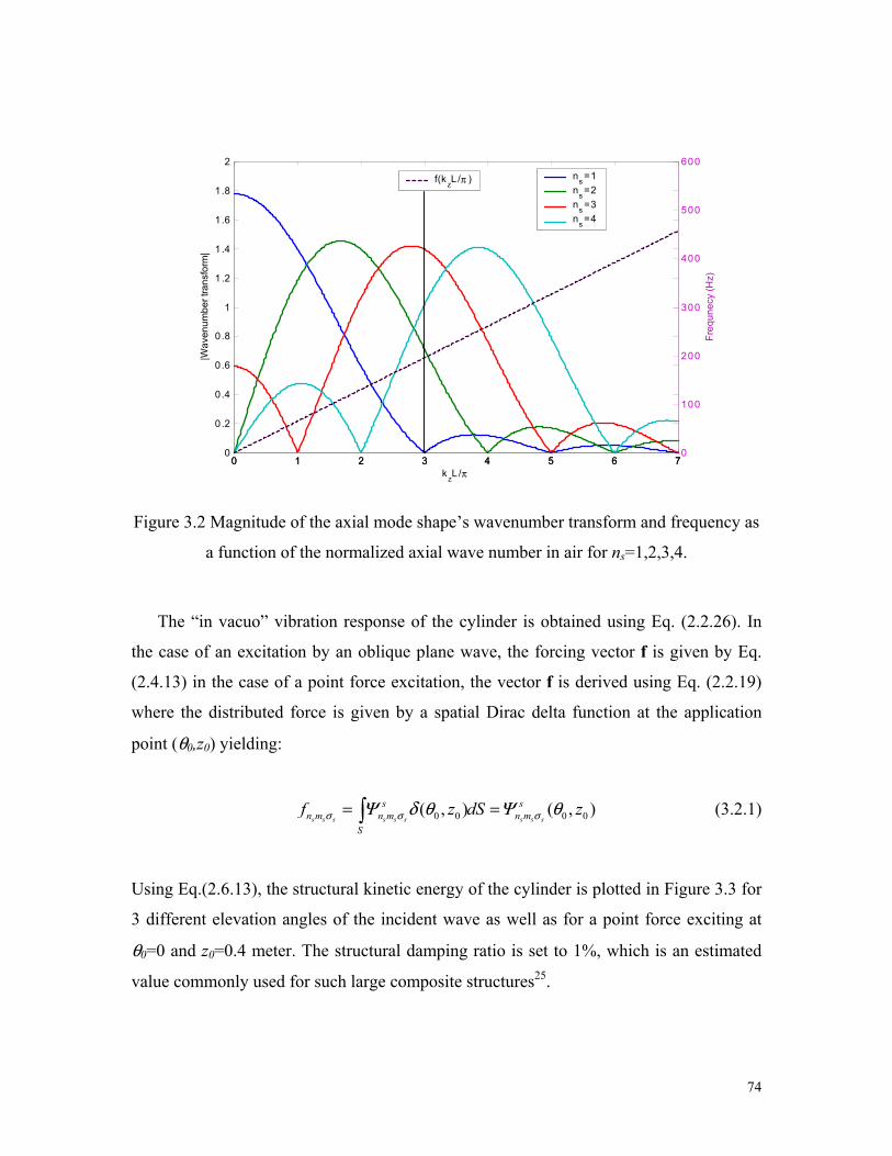
74
0 1 2 3 4 5 6 70
0.2
0.4
0.6
0.8
1
1.2
1.4
1.6
1.8
2
kzL /π
|Wav
enum
ber t
rans
form
|
ns =1ns =2ns =3ns =4
0 1 2 3 4 5 6 70
100
200
300
400
500
600
Freq
unec
y (H
z)
f(kzL /π )
Figure 3.2 Magnitude of the axial mode shape’s wavenumber transform and frequency as
a function of the normalized axial wave number in air for ns=1,2,3,4.
The “in vacuo” vibration response of the cylinder is obtained using Eq. (2.2.26). In
the case of an excitation by an oblique plane wave, the forcing vector f is given by Eq.
(2.4.13) in the case of a point force excitation, the vector f is derived using Eq. (2.2.19)
where the distributed force is given by a spatial Dirac delta function at the application
point (θ0,z0) yielding:
0 0 0 0( , ) ( , )s s s s s s s s s
s sn m n m n m
S
f z dS zσ σ σΨ δ θ Ψ θ= =∫ (3.2.1)
Using Eq.(2.6.13), the structural kinetic energy of the cylinder is plotted in Figure 3.3 for
3 different elevation angles of the incident wave as well as for a point force exciting at
θ0=0 and z0=0.4 meter. The structural damping ratio is set to 1%, which is an estimated
value commonly used for such large composite structures25.
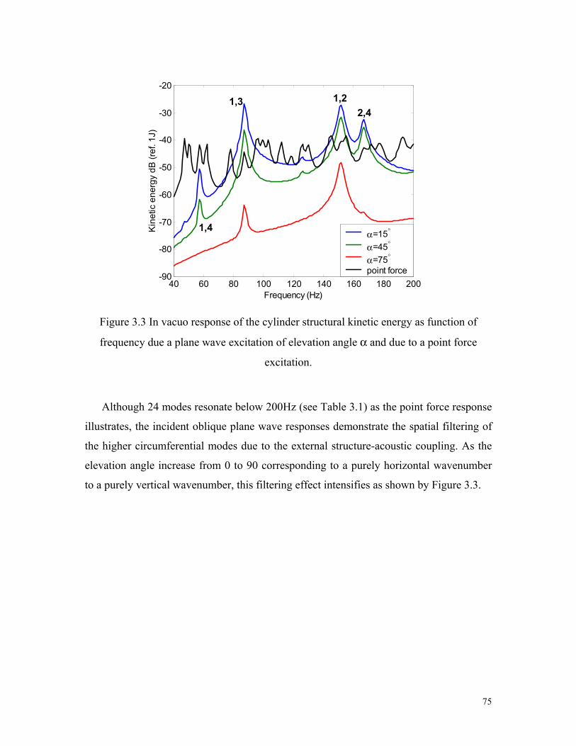
75
40 60 80 100 120 140 160 180 200-90
-80
-70
-60
-50
-40
-30
-20
Kin
etic
ene
rgy
dB (r
ef. 1
J)
Frequency (Hz)
α=15°
α=45°
α=75°
point force
1,3
1,4
1,2 2,4
Figure 3.3 In vacuo response of the cylinder structural kinetic energy as function of
frequency due a plane wave excitation of elevation angle α and due to a point force
excitation.
Although 24 modes resonate below 200Hz (see Table 3.1) as the point force response
illustrates, the incident oblique plane wave responses demonstrate the spatial filtering of
the higher circumferential modes due to the external structure-acoustic coupling. As the
elevation angle increase from 0 to 90 corresponding to a purely horizontal wavenumber
to a purely vertical wavenumber, this filtering effect intensifies as shown by Figure 3.3.

76
Axial order n Circumferential order m Natural frequency (Hz) 1 5 47.3 1 6 50.4 1 4 57.4 1 7 61.7 1 8 77.7 1 3 87.3 2 7 95.5 1 9 96.8 2 8 99.5 2 6 103.2 2 9 111.9 1 10 118.5 2 5 125.7 2 10 129.8 3 8 144.5 3 9 145.4 1 2 151.7 3 7 154.9 3 10 155.2 2 4 166.9 3 6 178.3 4 9 192.1 4 10 193.5 4 8 200.7
Table 3.1 Structural resonant frequency of the Boeing cylinder below 200Hz
3.2.2. Internal coupling
The structural acoustic coupling between bending waves on a plate and an acoustic
field has been extensively studied78,79. Typically, at low frequencies the bending waves
on a thin plate are slower than the acoustic wave speed (subsonic) and therefore do not
efficiently radiate sound. Only the boundaries, which make the plate finite, allow the
structure to couple effectively into the fluid in this subsonic frequency range. These
boundaries permits the aliasing of the high wavenumbers under the form of side lobes
into the low wavenumber region, as illustrated in Figure 3.2. This effect is also true of a
cylinder where the boundaries are largely responsible for coupling the structural vibration
to the acoustic cavity. Cylinders present an additional effect due to their curvature, which
couples the bending and the in-plane responses. Since the structure is very stiff in the “in-

77
plane” direction, this coupling, effectively speeds up the low order circumferential modes
that are the most coupled with the in-plane motion. This phenomenon, sometimes called
the membrane effect, can cause “supersonic” behavior at lower frequencies than would
be expected from a bending wave plate model. This is illustrated in Figure 3.4 where the
structure wavenumbers 2 2
nmn mkL Rπ = +
are plotted as a function of their natural
frequencies 2nm
nmf ωπ= and linked in n groups. The dispersion curves for the
equivalent sandwich plate without core shear kb(ω) and for the air k(ω) are also plotted.
As expected, below the coincidence frequency (kb=k), the bending response of the plate
is sub-sonic (kb>k) whereas the low circumferential order modes of the cylinder (m<5)
present a supersonic behavior (knm<k) due to the membrane effect. This effect is the
highest for the breathing modes m=0 and thus forces the first 10 breathing modes to
present a very similar natural frequency. Note that the equivalent sandwich plate appears
stiffer than the cylinder at high frequency due to neglecting the core shear78.
0 2 4 6 8 10 12 14 16 18 200
100
200
300
400
500
600
700
800
900
1000
1100
Freq
uenc
y (H
z)
structural wavenumber (1/meter)
Figure 3.4 Dispersion curves for the Boeing cylinder in ‘n’ groups and for the equivalent
infinite sandwich plate without core shear.
k=ω/c
n=1 n=2 n=6
increasing m
kb

78
The level of coupling between the structural mode of the cylinder and the acoustic
mode of its cavity is both spatial and frequency related. The spatial level is represented
by the coefficient of the coupling matrix C derived in Eq.(2.4.16). In order to visualize
both levels at the same time, Figure 3.5 shows two contour plots, one for the acoustic
modes and one for the structural modes, superimposed on each other as a function of their
axial and circumferential orders (note that only p=0 acoustic modes are plotted). The
contours represent the resonant frequencies for each of the modes, blue for acoustic
modes and red for structural modes. The modes only occur on the integer values of the
plot. Acoustic modes with higher orders have higher natural frequencies but for structural
modes, because of the membrane effect, this relationship between frequency and mode
order is distorted. The lowest natural frequencies are for m=5 to m=6 (lower right-hand
corner). As mentioned in section 2.4.2, the spatial coupling between acoustic and
structural modes is such that only like circumferential mode orders (m) couple and in the
axial direction (n) odd modes on the structure couple to even modes in the cylinder (and
visa-versa). Therefore each intersection on the grid represents a non-zero coupling
between two modes. The black line on the plots shows a line of equal natural frequency
of the structural and acoustic modes. Therefore the proximity of the grid points to this
line expresses the similarity in natural frequency of two spatially well-coupled modes.
The red dot on the plot highlight the cases where both high spatial and frequency
coupling occurs which results in large sound transmission. The problematic interactions,
are between the (1,2) structural mode and the (0,2,0) acoustic mode around 140Hz,
between the (2,3) and the (1,3,0) around 200Hz and between the (3,4) and the (2,4,0)
around 260Hz. This plot can be repeated for acoustic modes with a radial component (i.e.
p=1,2,3…) to form new frequency coincidence lines. The main result is that the majority
of coupling will come from modes that lie near to or to the left of the black line shown in
Figure 3.5.

79
0 1 2 3 4 5 6 70
1
2
3
4
5
6
circumferential mode order (m)
acou
stic
axi
al m
ode
orde
r (n)
4060
80
100
120
140
160
180
180
200
200
220
220
240
240
260
260280
280
300300
320
320
320
340
340
340360
360
360
380
380
380
400
420
420
440
440
460
520
6080
80
100
120
120
140
140
160
160
180
180
200
200
220
220
240
240
260
260
280
280
300
300
320
320
320
340
340
340
360
360
360
380
380
380
400
400
400
420
420
4
440
440
460
460
480
480
500
500
520
0 1 2 3 4 5 6 71
2
3
4
5
6
7
stru
ctur
al a
xial
mod
e or
der (
n s)
Figure 3.5 Contours of the structural and acoustic resonant frequencies as a function of
their mode orders.
The vibration and acoustic responses of the fully coupled system neglecting the
external fluid loading is obtained using Eq.(2.6.7) and Eq.(2.6.8) with Zr=0. Figure 3.6
shows the structural kinetic and acoustic potential energy of the cylinder excited by an
oblique plane wave (αi=70°). The acoustic damping is set to 1%. As pointed out by the
mode orders, the internal acoustic response as well as the vibration response, are both
composed of coupled acoustic resonances and structural resonances. Below 200Hz the
main transmission path is due to the high structural-acoustic coupling between the (1,2)
that resonates at 151Hz and (0,2,0) that resonates at 135Hz. Note that these two resonant
frequencies are pushed up and down respectively as the two modes interact. Figure 3.7
shows the structural kinetic and acoustic energy of the cylinder in the case of an annular
cavity of internal radius Ri=3ft. As the 0,2,0 resonant frequency is lowered to 102 Hz, the
coupling with the (1,2) structural mode is weaker and thus less energy is transmitted.

80
40 60 80 100 120 140 160 180 200-85
-80
-75
-70
-65
-60
-55
-50
-45
Ene
rgy
dB (r
ef. 1
J)
Frequency (Hz)
AcousticKinetic
1,0,0
0,1,0 1,1,0
0,2,0
2,1,0
1,2
2,2,0 1,3
Figure 3.6 Structural kinetic energy and acoustic potential energy of an empty cylinder excited by an oblique plane wave (αi=70°).
40 60 80 100 120 140 160 180 200-85
-80
-75
-70
-65
-60
-55
-50
-45
Ene
rgy
dB (r
ef.1
J)
Frequency (Hz)
AcousticKinetic
0,1,0 1,0,0 1,1,0
1,3 0,2,0
1,2
Figure 3.7 Structural kinetic energy and acoustic potential energy of an annular cylinder excited by an oblique plane wave (αi=70°).

81
3.2.3. Fluid loading effect
As detailed in section 2.2.4, the surrounding fluid couples the structural mode of same
circumferential order through the radiation impedance matrix Zr. Neglecting this cross
coupling by only considering the diagonal term of Zr, reveals the fluid loading effect on
each mode. This effect is two fold: the real part of the radiation impedance acts as a
damping term as energy is lost by acoustic radiation, whereas the imaginary part is mass-
like in the low frequencies. The additional damping ratio ξrad can be approximated for
each mode by
( )Re
2
rnnm nmrad
nmnm
ZM
ωξ
ω = . (3.2.2)
The additional mass, mrad, which lowers the mode natural frequencies, is obtained by
evaluating the slope of the radiation impedance at the low frequencies as
( )
0
Im rnnmrad
nm
d Zm
dω
ω=
−= . (3.2.3)
As the radiation impedance is linked to the coupling with the wavenumber in air it
depends on the vibration pattern of the cylinder (i.e the structural mode shapes) and on
the frequency. Figure 3.8 shows the real and imaginary part of the normalized radiation
impedance for three low order structural modes. The scaled modal mobilities indicating
the mode natural frequencies are superimposed in dotted lines. The fluid loading effect
appears more important for the lower order circumferential modes. Table 3.2 lists the
value of the additional radiation damping ratio and the radiation mass in percent of the
mass of the cylinder for different modes.

82
Mode order Approximated radiation impedance effect
Axial (n) Circumferential (m) Damping ratio (%) Additional mass (% of cylinder mass)
1 4 0.0 9.5 1 3 1.1 11.5 1 2 6.0 14.0 2 4 2.6 8.2 2 3 5.3 9.6 1 1 2.1 16.2 2 2 2.9 11.3 2 1 2.0 13.8 1 0 1.6 36.8 2 0 1.8 16.4
Table 3.2 Additional damping ratio, and mass ratio for the Boeing cylinder modes due to
the fluid loading effect.
The structural kinetic energy of the cylinder is plotted for three different
configurations in Figure 3.9: without the external loading (“in vacuo”) as in Figure 3.6,
with the radiation impedance corresponding to Eq.(2.6.7) (“fluid loaded”), and with using
only the diagonal terms of Zr (“diagonally fluid loaded”). For this particular structure
below 200Hz, the cross modal coupling through the radiation impedance matrix appears
negligible, and so only the diagonal terms of Zr will be used in the simulations. As
expected the resonance of the 1,3 mode is shifted down and the 1,2 mode peak at 160Hz
and its coupled acoustic resonance at 120Hz are significantly damped compare to the “in
vacuo” case. Figure 3.9 also shows how these fluid loading effects modify the acoustic
potential energy response. Note that in absence of notification, the reference used to plot
frequency response in decibel is assumed to be 1 unit.

83
0 20 40 60 80 100 120 140 1600
10
20
30
Frequency (Hz)
-Im[Z
r nnm
/ ρc]
1 31 22 41 0
40 60 80 100 120 140 160 180 2000
10
20
30
Re[
Zr nnm
/ ρc]
Frequency (Hz)
1 31 22 41 0
Figure 3.8 Real and imaginary part of the normalized radiation impedance as function of
frequency for three different modes with scaled modal response (dotted line).
50 70 90 110 130 150 170 190-85
-80
-75
-70
-65
-60
-55
-50
-45
Kin
etic
ene
rgy
(dB
)
Frequency (Hz)
in vacuo fluid loaded diagonally fluid loaded
50 70 90 110 130 150 170 190-85
-80
-75
-70
-65
-60
-55
-50
-45
Aco
ustic
pot
entia
l ene
rgy
(dB
)
Frequency (Hz)
in vacuo fluid loaded diagonally fluid loaded
Figure 3.9 Influence of the external fluid loading on the structural kinetic energy and the
acoustic potential energy of the cylinder under oblique plane wave excitation (αi=70°).

84
3.2.4. Model validation
The composite cylinder prototype shown in Figure 3.10 was built by Boeing and
shipped to Virginia Tech in September 2001. A dolly was built that allowed the cylinder
to move in an upright position and to be lowered to the ground for testing. The bottom
and top end cap are made of 5.5” thick plywood in which the edges of the cylinder are
slotted. Three aluminum I-beams reinforce each end cap. Twelve threaded rods evenly
spaced along the circumference secure the bottom and the top end cap together. In order
to evaluate the accuracy of the model, several experiments were done.
Figure 3.10 Boeing composite cylinder on its dolly with the 5 rings of 30 accelerometers.
Validation of the acoustic cavity model
To determine the behavior of the acoustic cavity, a speaker was placed inside the
cylinder and driven with 40-200Hz band passed white noise. In order to measure the

85
volume velocity (VV) of this source a microphone was placed into the speaker cabinet of
volume Vs as shown in Figure 3.11. As long as the frequency of excitation is well below
the first mode of the cabinet the pressure inside (pin) is uniform and proportional to the
speaker volume velocity80 u:
2( ) ( )sin
i Vu pc
ωω ωρ
= (3.2.4)
Three rings of five microphones positioned at 19, 54, 92 inches from the bottom and
12 inches from the wall were used to obtain a spatial average of the acoustic pressure
inside the cylinder. The transfer functions between all of the 15 microphones and the
microphone placed inside the speaker cabinet were acquired. This technique allows the
dynamics of the disturbance speaker to be removed from the transfer functions.
Mic Speaker
12’’ 12’’ Mic
cable
Power cable
12’’ Vs
Figure 3.11 Picture and schematic of the volume velocity speaker with internal
microphone.
Using the fully coupled model developed in section 2.6, the acoustic pressure is
reconstructed at the 15 microphones locations. Figure 3.12 shows the experimental and
predicted acoustic response at two microphones locations. The damping of the first 9
acoustic modes is evaluated from the measured transfer function and used in the model.

86
The typical acoustic damping ratios used to match the model range from 0.5 to 1 %.
Figure 3.13 presents the measured and predicted SPL per unit volume velocity of the
source obtained by averaging the 15 microphone responses. For both Figure 3.12 and
Figure 3.13 the agreement between the experiment and the simulation is satisfactory.
40 60 80 100 120 140 160 180 200100
120
140
160
180microphone 9
SP
L/V
V (d
B re
f 2x1
0- 5)
Frequency (Hz)
experimentcode
40 60 80 100 120 140 160 180 200-200
-100
0
100
200
phas
e (d
egre
e)
Frequency (Hz)
experimentcode
40 60 80 100 120 140 160 180 200100
120
140
160
180microphone 13
SP
L/V
V (d
B re
f 2x1
0- 5)
Frequency (Hz)
experimentcode
40 60 80 100 120 140 160 180 200-200
-100
0
100
200
phas
e (d
egre
e)
Frequency (Hz)
experimentcode
Figure 3.12 Experimental and predicted acoustic response at two microphones locations

87
40 60 80 100 120 140 160 180 200130
135
140
145
150
155
160
165
170
SP
L/V
V (d
B re
f 2x1
0- 5)
Frequency (Hz)
experimentcode
Figure 3.13 Experimental and predicted spatially averaged SPL (15 microphones) per
volume velocity (VV).
Using the experimental data the amplitude of NM modes can be extracted using an
inverse technique81. At each frequency the pressure at the 15 microphones is represented
in matrix form as:
p = Φ a , (3.2.5)
where a is the NMx1 vector of complex mode amplitudes and the 15xNM matrix Φ defines
the NM mode shape values at the 15 microphone positions. The elements of Φ are
obtained using the theoretical mode shapes given in Eq.(2.3.12). The 15x1 vector is
composed of the measure acoustic pressure response at the 15 microphones. If the
number of mode NM chosen to describe the pressure field is equal to the number of
microphones, the matrix Φ is square and thus the mode amplitudes are given by
88
-1a = Φ p (3.2.6)
However, depending on the chosen microphone locations, two different modes can render
Φ singular by having two linearly dependent columns. In this particular case, since the 15
microphones monitor only one radial position, the 1,0,0 and 1,0,1 acoustic modes are
spatially identical at the microphone positions and thus cannot be simultaneously
included in the modal set. Furthermore, because of errors associated with the microphone
locations as well as with the theoretical mode shapes, it is usually better to use an over-
determine system with more equations than unknowns, that is using more sensor
measurements than modes. The extracted mode amplitudes become then a least square
approximated solution expressed as:
T -1
a = Φ Φ Φp (3.2.7)
This technique applied to the 15 measured acoustic responses with 9 acoustic modes
allows assigning to each peak of the acoustic response a mode order. The extracted and
the predicted amplitude for three different modes are compared in Figure 3.14. Table 3.3
lists the mode order and natural frequencies of the dominant acoustic peak below 200Hz
obtained experimentally, computed with Eq. (2.3.16) (hard wall condition) and obtained
using the fully coupled model. Except for the 0,2,0 mode that shows three damped peaks
resulting from the coupling to the 1,2 structural mode (164Hz) and the 2,2,0 acoustic
mode (188Hz), the natural frequencies using Eq.(2.3.16) are fairly close to the fully
coupled model predictions. The extraction of the 0,2,0 modal response from the
experimental data does not permit a clear identification of the three coupled frequencies
observed with the model.

89
40 60 80 100 120 140 160 180 2000
20
40
60
80
Mod
e am
plitu
de (d
B/V
V)
Frequency (Hz)
1 0 0 exp 1 0 0 code
40 60 80 100 120 140 160 180 200-20
0
20
40
60
Mod
e am
plitu
de (d
B/V
V)
Frequency (Hz)
1 1 0 exp 1 1 0 code
40 60 80 100 120 140 160 180 2000
20
40
60
80
Mod
e am
plitu
de (d
B/V
V)
Frequency (Hz)
2 0 0 exp 2 0 0 code
Figure 3.14 Mode amplitudes extracted from the microphone data and predicted by the
numerical code.
Mode order Natural frequency (Hz)
n m p Measured Eq. 2.2.16 Fully coupled 1 0 0 64.0 62.8 63.0 0 1 0 82.0 82.5 82.0 1 1 0 103.2 103.6 103.0 2 0 0 125.6 125.6 125.5 0 2 0 … 136.8 121,164,188 2 1 0 148.5 150.3 149.4 1 2 0 146,149 150.5 149.0 2 2 0 183.0 185.7 188.5
Table 3.3 List of measured, theoretical and fully coupled acoustic natural frequencies.

90
Validation of the structural model
A shaker test was used to identify natural frequency and the mode shapes of the
cylinder. A 50lb shaker positioned at [θ=0, z=23”] excited the cylinder. To avoid stress
concentration, the stinger of the shaker was threaded into a 2” diameter curved aluminum
disk glued on the cylinder. A total of 5 rings of 30 point each meshed the surface (see
Figure 3.10). The rings were positioned every 20” starting from the bottom of the
cylinder. The input force was measured with a force transducer placed between the
cylinder and the shaker, which was driven with 40-500Hz band passed white noise.
Transfer functions between the input force and the acceleration at the 150 locations in
addition to the excitation location were acquired. As for the validation of the acoustic
cavity, the fully coupled model was used to predict the velocity response at the
accelerometer positions. Figure 3.15 shows the velocity response per unit force at the
excitation location and at position 65 in the 3rd ring, 60° from the excitation point. The
structural damping ratios are adjusted around the 1% value for a better match with the
measurement. Figure 3.16 compares the spatially averaged velocities per unit force using
the 151 measured transfer functions with the model predictions. Except for under
predicting the first three resonant frequencies, the fully coupled model is in good
agreement with the measurement. The discrepancies can be due to the free-field radiation
assumption, as the data was acquired indoors. The theoretical boundary conditions, which
determine the natural frequencies, are also difficult to recreate experimentally. To
identify the peaks with the modes of the structure, the same inverse method used for the
acoustic cavity can be applied on the accelerometer transfer functions to extract the
structural mode amplitudes. Figure 3.17 shows for three different modes the experimental
and predicted amplitude. To facilitate this modal identification, another modal
decomposition technique, the spatial Fourier (or wavenumber) transform, can be applied
to 30 experimental or predicted velocities belonging to a particular ring. The result of this
transform is visualized as a contour plot of the velocity amplitudes as a function of both
frequency and circumferential mode order. As for a time-frequency Fourier transform,
the information is divided into a symmetric an antisymmetric content with respect to the
origin. Since the excitation position is taken as the angle origin, only modes with

91
orientation order σs=0 corresponding to a cosine circumferential variation are expected to
be excited. Figure 3.18 presents the symmetric components of the wavenumber transform
applied to the lower ring for both the measured and predicted response. The amplitude
are normalized by their maximum value and plotted with a logarithmic scale. For both the
theoretical and experimental results, the modes for each axial order n lie on a “u” shaped
curve characteristic of cylinders dispersion relationship as previously observed in Figure
3.4. Figure 3.18 also shows a good agreement between the model prediction and the
experiment.

92
40 60 80 100 120 140 160 180 200-80
-70
-60
-50
-40
-30
Frequency (Hz)
Excitation point
|vel
ocity
/forc
e| (d
B)
exp code
40 60 80 100 120 140 160 180 200-100
-50
0
50
100
phas
e (d
egre
e)
Frequency (Hz)
exp code
40 60 80 100 120 140 160 180 200-100
-80
-60
-40
Frequency (Hz)
Position 65
|vel
ocity
/forc
e| (d
B)
exp code
40 60 80 100 120 140 160 180 200-200
-100
0
100
200
phas
e (d
egre
e)
Frequency (Hz)
exp code
Figure 3.15 Experimental and predicted velocity response per unit force at the excitation
location and at position 65 (3rd ring up).

93
40 60 80 100 120 140 160 180 200-75
-70
-65
-60
-55
-50
-45
mea
n ve
loci
ty s
quar
ed/fo
rce
(dB
/N)
Frequency (Hz)
exp code
Figure 3.16 Experimental and predicted mean velocity squared per unit force (151
positions).

94
40 60 80 100 120 140 160 180 200
-120
-100
-80
-60
Mod
e am
plitu
de (d
B/N
)
Frequency (Hz)
1 6 exp 1 6 code
40 60 80 100 120 140 160 180 200
-120
-100
-80
-60
Mod
e am
plitu
de (d
B/N
)
Frequency (Hz)
2 10 exp 2 10 code
40 60 80 100 120 140 160 180 200
-120
-100
-80
-60
Mod
e am
plitu
de (d
B/N
)
Frequency (Hz)
3 11 exp 3 11 code
Figure 3.17 Experimental and predicted modal amplitudes.
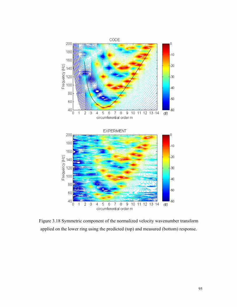
95
Figure 3.18 Symmetric component of the normalized velocity wavenumber transform
applied on the lower ring using the predicted (top) and measured (bottom) response.
96
Validation of the sound transmission
The acoustic pressure inside the cylinder subjected to the shaker excitation was also
measured at 96 positions covering 4 axial, 2 radial, and 12 angular different locations.
The 96 transfer functions between the microphones and the input force provided an
estimation of the averaged internal SPL per unit point force. Theoretically, because of the
coupling matrix properties and the few low circumferential order structural modes below
200Hz, the internal SPL should be limited to acoustic modes resonating in the bandwidth.
However, the comparison between the measured and predicted SPL plotted in Figure 3.19
in the top graph shows a relatively strong disagreement. The experimental spectrum
presents more peaks and higher amplitudes of the 0 and 1 circumferential order acoustic
modes at 60, 100 and 145Hz. the bottom graph of Figure 3.19 illustrates, these
discrepancies are attenuated by using a “noisy” coupling matrix which is obtained by
adding to each element of C a normally distributed random number of variance equals to
1% of cylinder’s surface. The acoustic transmission for this particular case seems very
sensitive to the imperfections in the mode shapes and boundary conditions that couple all
the modes together.

97
40 60 80 100 120 140 160 180 20050
60
70
80
90
100Theoretical coupling matrix
SP
L/fo
rce
(dB
ref 2
x10-5
)
Frequency (Hz)
exp code
40 60 80 100 120 140 160 180 20050
60
70
80
90
100Noisy coupling matrix
SP
L/fo
rce
(dB
ref 2
x10-5
)
Frequency (Hz)
exp code
Figure 3.19 Measured and predicted internal SPL per unit input force using the
theoretical coupling matrix (top) and the “noisy” coupling matrix (bottom).
3.2.5. Fairing model
In this section, the different elements of the fairing model are presented. The
similarities with the cylinder are highlighted and the particularities due to the finite
element base of the model are explained.
External coupling
The fairing being an axisymetric structure, causes the orthogonal mode shapes
computed by the finite element model to appear in pairs of circumferential mode order as

98
observed in a perfect cylinder. As shown in Figure 3.20 the connection between the
cylindrical and the cone section represents a nodal line for most of the mode shapes.
Consequently, the motion of in the fairing cylindrical section can be approximated using
the axial and circumferential order of a simply supported cylinder. The wavenumber
transform performed on velocity responses to a point force excitation (z=0.15m) at 36
points around the circumference confirms this similar behavior. Figure 3.21 shows that
the wavenumber transform fairing presents the “u” shaped curve characteristic of
cylinders dispersion relationship observed in Figure 3.18.
Figure 3.20 Fairing structural mode shapes with the corresponding cylindrical section
mode order.

99
Figure 3.21 Circumferential wavenumber transform of the fairing velocity response to a
point force.
In order to compute the fairing response, the external acoustic excitation was chosen
to be representative of the full-scale tests detailed in section 4.4. Using the equivalent
source method presented in section 2.7.2, the external acoustic field on the fairing
generated by twelve speakers modeled as acoustic monopoles of constant volume
acceleration was computed. Figure 3.24 shows the resulting pressure distribution on the
fairing at 70Hz as well as the location of the speakers.

100
Figure 3.22 External pressure distribution on the fairing due to eight speakers at 70Hz.
Fluid loading effect approximation
The external coupling between the fairing and the external acoustic field differs from
the coupling between a cylinder and a plane wave excitation that was obtained
analytically. To avoid a complex and cumbersome numerical calculation of the fairing
radiation impedance, only its cylindrical section is considered to approximate the fluid
loading effects. Using the derivation in 3.2.3 and the mode orders describing the
cylindrical section motion, Eq. (3.2.2) and (3.2.3) approximate the additional damping
and mass effect of the external fluid on the fairing modes. This external damping ratio is
added to the structural damping characteristic of the fairing composite construction. As
an exact measurement of this quantity is complex and not crucial for the numerical
predictions, the structural damping is set to 1%. Table 3.4 shows the approximated
damping and mass effect of the fluid loading for the most affected modes.
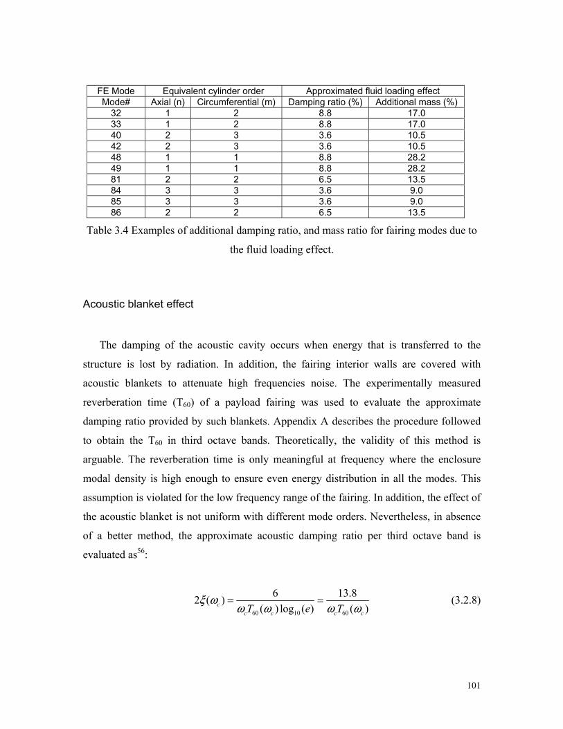
101
FE Mode Equivalent cylinder order Approximated fluid loading effect Mode# Axial (n) Circumferential (m) Damping ratio (%) Additional mass (%)
32 1 2 8.8 17.0 33 1 2 8.8 17.0 40 2 3 3.6 10.5 42 2 3 3.6 10.5 48 1 1 8.8 28.2 49 1 1 8.8 28.2 81 2 2 6.5 13.5 84 3 3 3.6 9.0 85 3 3 3.6 9.0 86 2 2 6.5 13.5
Table 3.4 Examples of additional damping ratio, and mass ratio for fairing modes due to
the fluid loading effect.
Acoustic blanket effect
The damping of the acoustic cavity occurs when energy that is transferred to the
structure is lost by radiation. In addition, the fairing interior walls are covered with
acoustic blankets to attenuate high frequencies noise. The experimentally measured
reverberation time (T60) of a payload fairing was used to evaluate the approximate
damping ratio provided by such blankets. Appendix A describes the procedure followed
to obtain the T60 in third octave bands. Theoretically, the validity of this method is
arguable. The reverberation time is only meaningful at frequency where the enclosure
modal density is high enough to ensure even energy distribution in all the modes. This
assumption is violated for the low frequency range of the fairing. In addition, the effect of
the acoustic blanket is not uniform with different mode orders. Nevertheless, in absence
of a better method, the approximate acoustic damping ratio per third octave band is
evaluated as56:
60 10 60
6 13.82 ( )( ) log ( ) ( )c
c c c cT e Tξ ω
ω ω ω ω= (3.2.8)

102
The resulting third octave band damping ratios are then curved fitted in the frequency
band of interest with a 4th order polynomial to extrapolate their value at the natural
frequency of the acoustic modes. In the 30-120Hz, the damping ratio only varies from 0.9
to 1.5% as seen in Figure 3.23.
40 60 80 100 1200.8
1
1.2
1.4
1.6
Frequency (Hz)
Dam
ping
ratio
(%) 1/3 octave from experimental T60
curve-fit
Figure 3.23 Acoustic damping ratio obtained from 1/3 octave T60 measurement.
Finally, as the foam treatment represents 10% of fairing mass, the structural natural
frequencies of the bare fairing obtained with the finite element are multiply by 11.1 to
drop them accordingly.
Internal coupling and mode selection
As the fairing model comprise 1109 structural modes and 293 acoustic modes, a
selection of the most important modes is necessary to keep computational time low. This
modal selection is a relatively complex process as it involves different levels of coupling,
which do not present close-form expressions as opposed to the analytical cylinder
formulation. The first selection consists in including all the acoustic and structural modes
that resonate in the frequency band slightly larger than the one of interest, in this
particular case up to 130Hz. This set of mode is insufficient to accurately describe the
acoustic response as it discards two main transmission paths. The first and most
important one comes from the forcing of an acoustic mode resonant in the bandwidth by

103
a structural mode resonant outside the band (as mentioned in section 2.4.2). The second
path comes from an acoustic mode resonant outside the band that is forced by a structural
mode resonant inside the band. To select the most important modes, the individual
response of each acoustic mode, n, to each structural mode, m, is computed and
integrated over the frequency band of interest.
130
30
( ) ( , ) ( ) ( )Hz
a snm n m m
Hz
A C n m A F dβ ω ω ω ω= ⋅ ⋅ ⋅∫ (3.2.9)
The resulting value nmβ , which corresponds to the acoustic energy transmitted over the
band of a particular structural-acoustic mode combination, is used to sort the modes in
term of their energy contribution. Figure 3.24 shows the repartition of nmβ with respect to
the structural and acoustic natural frequencies. In this particular case only the six most
important modes are retained to create the modal subset. As illustrated by the rectangular
box, the first transmission path described previously largely dominates even over the
coupling between structural and acoustic modes both resonant in the band as in the case
of the cylinder.

104
Figure 3.24 Overall coupling level between structural acoustic modes.
Figure 3.25 shows the velocity and acoustic response up to 110Hz using the complete
modal set and the resulting modal subset comprising 288 structural and 79 acoustic
modes with frequency up to 295 and 130Hz respectively. The differences in the velocity
response between the two modal sets are negligible since all the modes below 130Hz are
included and the second transmission path is marginal. As the first transmission path
dominates across the band, the reduction of the structural modal set induces for particular
acoustic modes slightly bigger differences in the response. These discrepancies never
exceed 1.5 dB at the peak; on the other hand simulation with the modal subset are 80
times faster which is a considerable advantage when using the genetic algorithm (section
3.5.2).
Control region
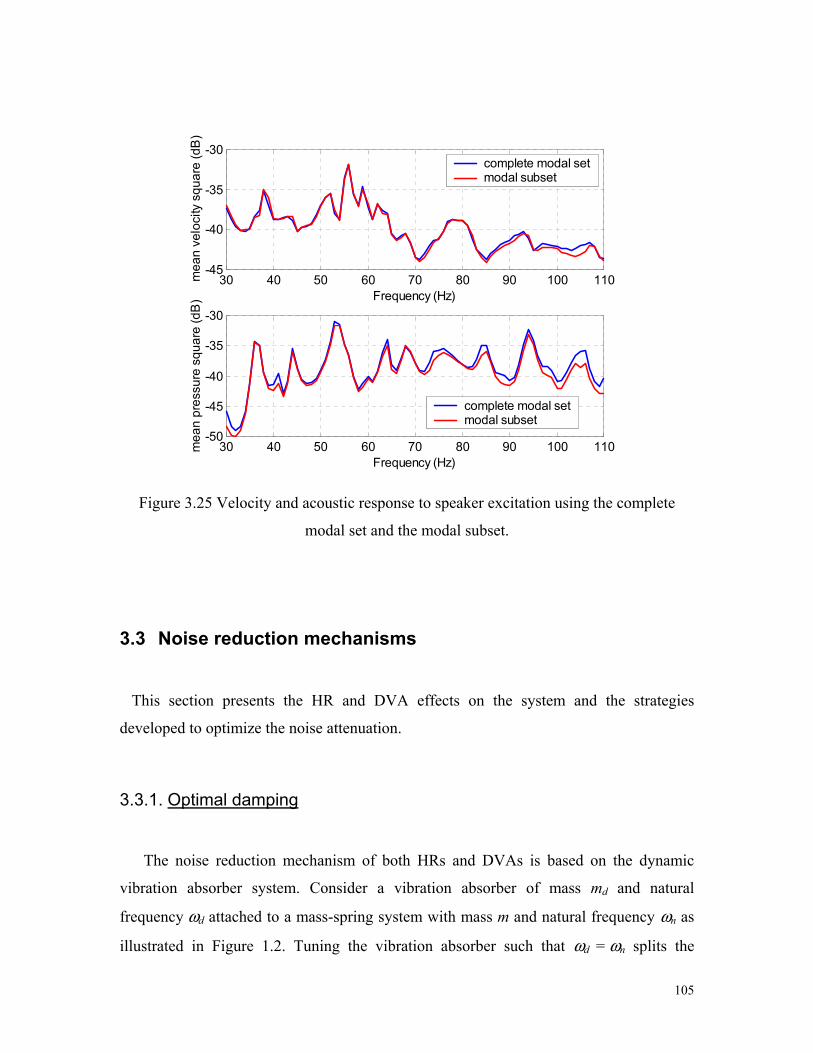
105
30 40 50 60 70 80 90 100 110-45
-40
-35
-30
Frequency (Hz)
mea
n ve
loci
ty s
quar
e (d
B)
complete modal setmodal subset
30 40 50 60 70 80 90 100 110-50
-45
-40
-35
-30
Frequency (Hz)
mea
n pr
essu
re s
quar
e (d
B)
complete modal setmodal subset
Figure 3.25 Velocity and acoustic response to speaker excitation using the complete
modal set and the modal subset.
3.3 Noise reduction mechanisms
This section presents the HR and DVA effects on the system and the strategies
developed to optimize the noise attenuation.
3.3.1. Optimal damping
The noise reduction mechanism of both HRs and DVAs is based on the dynamic
vibration absorber system. Consider a vibration absorber of mass md and natural
frequency ωd attached to a mass-spring system with mass m and natural frequency ωn as
illustrated in Figure 1.2. Tuning the vibration absorber such that ωd = ωn splits the

106
resonance of the system into two new resonances of similar amplitude either side of ωn.
The bigger the mass ratio, the further apart the two resonances of the coupled system
appear. By adding damping to the absorber, (i.e. between the system and the absorber
mass), both ‘new’ resonances are damped and significant broadband attenuation can be
achieved. Depending on the type of excitation, several formulas for damping ratios lead
to optimal vibration reduction28,29. For a wide band random excitation, the optimal
damping ratio d
optς derived by Korenev and Reznikov29 to minimize the primary system’s
velocity is expressed as
12 1d
opt νςν
=+
, (3.3.1)
where ν=md/m. Once coupled to a continuous structure of mass M, the effective mass
ratioν is weighted by the normalized mode shape squared at the absorber location (θ0,z0)
20 0[ , ]
s s s
s dn m
mν (θ z )MσΨ (3.3.2)
The coupling between a HR of volume Vh and an acoustic mode of an enclosure of
volume V obeys the same mechanisms. By analogy with den Hartog’s optimized dynamic
absorber29, Fahy and Schofield56 derived an optimal HR damping level opthς as a solution
of
4 3 2
2 1 1 12 1 02 2 2nmpopt opt opt
h h h
µ µξ µς ς ς
+ + − =
, (3.3.3)
where nmpξ is the modal damping of the enclosure and µ the effective volume ratio given
by
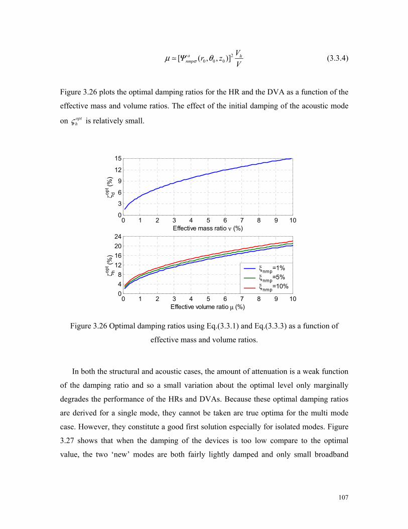
107
20 0 0[ ( , , )]a h
nmpVr zVσµ Ψ θ (3.3.4)
Figure 3.26 plots the optimal damping ratios for the HR and the DVA as a function of the
effective mass and volume ratios. The effect of the initial damping of the acoustic mode
on opthς is relatively small.
0 1 2 3 4 5 6 7 8 9 100
3
6
9
12
15
Effective mass ratio ν (%)
ζ dopt (%
)
0 1 2 3 4 5 6 7 8 9 10048
12162024
Effective volume ratio µ (%)
ζ hopt (%
)
ξnmp=1% ξnmp=5% ξnmp=10%
Figure 3.26 Optimal damping ratios using Eq.(3.3.1) and Eq.(3.3.3) as a function of
effective mass and volume ratios.
In both the structural and acoustic cases, the amount of attenuation is a weak function
of the damping ratio and so a small variation about the optimal level only marginally
degrades the performance of the HRs and DVAs. Because these optimal damping ratios
are derived for a single mode, they cannot be taken are true optima for the multi mode
case. However, they constitute a good first solution especially for isolated modes. Figure
3.27 shows that when the damping of the devices is too low compare to the optimal
value, the two ‘new’ modes are both fairly lightly damped and only small broadband

108
noise reduction is achieved. Alternatively, when the damping is too high, the devices
become uncoupled from the mode and no longer dissipate energy.
70 75 80 85 90-76
-74
-72
-70
-68
-66
-64
-62
-60
kine
tic e
nerg
y (d
B)
Frequency (Hz)
bare ζd=0.01 ζd
opt=0.07ζd=0.25
70 75 80 85 90-85
-80
-75
-70
-65
-60
-55
-50
acou
stic
ene
rgy
(dB
)
Frequency (Hz)
bare ζh=0.01 ζh
opt=0.08ζh=0.25
Figure 3.27 Influence of the DVA and HR damping ratios on the kinetic and acoustic
energy.
In both cases the devices were split into several identical units distributed evenly
around the circumference and tuned to the resonant frequency of the targeted mode.
Consequently, the number of device per ring has to be greater than twice the
circumferential order to avoid collocation of the units with nodes of vibration. The
effective mass or volume ratio of a ring is computed using only the axial mode shape
component and is weighted by 1/εm since half the mass or volume of the devices
effectively acts on circumferential modes greater than zero. In Figure 3.27 the DVA
treatment weighs 1% of structure’s mass and is composed of 13 1.5” by 2.5” DVAs
attached at z=L/2. The HR treatment representing 1% of the cavity’s volume is split into 7
units also positioned in the middle of the cylinder.
109
3.3.2. Devices are used in rings.
Multiple devices are used for two reasons. First, using a symmetric ring of devices
allows the treatment to be independent of the azimuth angle θi of the incident field, which
is assumed to be unknown. Second, the devices act as discontinuities that can couple
modes together by shifting energy from one circumferential mode to another. For
instance, a ring of Nd DVAs targeting a mode of circumferential order ms=i redistributes
the energy to all | |s dm i qN= ± modes where q is an integer. Thus, a DVA treatment is
likely to excite structural modes that are not forced by the incident acoustic field. The
closer the resonant frequency of the | |s dm i qN= ± mode is to the DVAs’ tuning
frequency, the higher the excitation. Therefore, a large number DVAs and HRs per ring
ensures a weak modal coupling since only modes with greatly different circumferential
order, which in most cases implies greatly different resonant frequencies, can interact. To
demonstrate this, Figure 3.28 shows the amplitude of the 1,2 and 1,7 structural modes
with two different treatment designed to target the 1,2 mode of the Boeing cylinder. The
tuning and the total mass of the DVAs (4% of the cylinder’s mass) remain the same for
both treatments. Only the number of DVAs per ring differs from 13 to 5. This shows that
when 5 DVAs per ring are used, the performance on the 1,2 mode is reduced compare to
the 13 DVAs per ring treatment. In addition, the 5 DVAs per ring treatment increased the
amplitude of 1,7 mode by 40 dB, compared to the bare or the 13 DVAs per ring treated
cylinder.

110
40 60 80 100 120 140 160 180 200-60
-50
-40
-30
1,2
Mod
e (d
B)
bare 5 DVA per ring 13 DVA per ring
40 60 80 100 120 140 160 180 200-140
-120
-100
-80
-60
-40
1,7
Mod
e (d
B)
bare 5 DVA per ring 13 DVA per ring
Figure 3.28 Influence of the number of DVA per ring on the amplitude of the 1,2 and 1,6
structural mode.
3.3.3. Influence of the DVA mass and HR volume.
As mentioned in section 2.5.1, the effect of a DVA on the vibration response is
proportional to the DVA to structure mass ratio. Likewise, the effect of a HR on the
acoustic response is proportional to the HR to cavity volume ratio. To illustrate this
Figure 3.29, compare the performance of DVA and HR treatment on an isolated mode for
different mass and volume ratio. In each case the devices are optimally damped with
respect to their mass/volume ratios and to the shape of the mode they are targeting. This
illustrates the existing trade-off between the weight and volume of a treatment and its

111
performance. Therefore in practice, the constraints imposed on the devices define an
upper bound for the noise attenuation.
70 75 80 85 90-76
-74
-72
-70
-68
-66
-64
-62
-60
kine
tic e
nerg
y (d
B)
Frequency (Hz)
bare md=9% md=1% md=0.2%
70 75 80 85 90-80
-75
-70
-65
-60
-55
-50
acou
stic
ene
rgy
(dB
)
Frequency (Hz)
bare Vh=9% Vh=1% Vh=0.2%
Figure 3.29 Influence of the DVA mass and HR volume in percent of the total mass and
total volume of the cylinder on the kinetic and acoustic energy.
3.3.4. Experimental validation.
In order to validate the model predictions, and demonstrate the effectiveness of the
DVAs and the HRs to reduce the vibration and the acoustic response, several experiments
were conducted on the cylinder prototype.
DVA validation
A treatment composed of 15 DVAs was designed to target the 1,7 mode of the
cylinder, which resonate at 61.5Hz. Each DVAs was built using a 2” thick 3”x5” block of
polyurethane acoustic foam on top of which was glued a metallic plate as shown in
Figure 3.30. Each DVA was then tuned, using the experimental set-up described in

112
Figure 3.31. The transfer function between two accelerometers one attached to the shaker
base the other attached to the DVA mass layer was curved fitted to a single degree
freedom response to extract the device’s natural frequency and damping ratio. To achieve
the desired frequency, the mass layer and the thickness of the foam can be varied. For a
given type of foam and footprint, the thinner the foam layer is, the stiffer. The damping
ratio produced by structural losses in the acoustic foam as it compresses is harder to
control. Using different types of foam leads to different damping levels. The particular
type used in this experiment provides a damping ratio of around 7%.
Acoustic foam
Mass layer
Acoustic foam
Mass layer
Figure 3.30 Example of a 3”x5” DVA made with 2” thick polyurethane foam.
Shaker
Rigid platform
FoamTape/Glue
Mass layer
A
B
band passed white noise
DVA
Accelerometer
Shaker
Rigid platform
FoamTape/Glue
Mass layer
A
B
band passed white noise
DVA
Accelerometer
Figure 3.31 Experimental set-up used to tune DVA.

113
The 15 DVAs were glued on the inner wall of the bare cylinder at z=L/2. The cylinder
was excited by a shaker in same configuration described in section 3.2.4. The transfer
functions between the shaker input and the 150 accelerometers meshing the cylinder
surface were used to get a spatial averaged vibration response. In addition to a good
agreement between the measured and predicted response, Figure 3.32 shows that the
DVAs drastically reduce the amplitude of not only the targeted 1,7 mode but all the
structural modes resonating in the 50-80Hz region. The total mass of the treatment was
2.5Kg, which represents 3.3% of the cylinder’s mass. This treatment leading to a
vibration attenuation of 9.2 dB from 50Hz to 80Hz also reduces the acoustic level in the
same band by 10dB as Figure 3.33 shows. Therefore, this experiment validates the
modeling techniques used to implement the DVA in the fully coupled modal model.
40 50 60 70 80 90 100 110 120-75
-70
-65
-60
-55
-50
-45
Frequency (Hz)
mea
n ve
loci
ty s
quar
ed/fo
rce
(dB
/N)
measured DVA predicted DVA measured bare predicted bare
9.2 dB (measured)
Figure 3.32 Measured and predicted vibration response of the bare (dotted line) and the
DVAs treated cylinder (solid).

114
40 50 60 70 80 90 100 110 12050
55
60
65
70
75
80
85
90
SP
L/fo
rce
(dB
ref 2
x10-5
)
Frequency (Hz)
measured DVA predicted DVA measured bare predicted bare
10 dB (measured)
Figure 3.33 Measured and predicted acoustic response of the bare (dotted line) and the
DVAs treated cylinder (solid).
HR validation
The resonators as shown in Figure 3.34 were designed using cardboard mailing tube
enclosed by plastic end-cap. The throat was cut into one of the end-caps. The neck made
of aluminum flexible hose was folded inside the tube to allow a more compact design. In
addition to the HR natural frequency, the internal neck creates other resonances usually
encountered in mufflers. However, these resonances appear at much higher frequencies
and therefore do not affect the HR performance. The HRs are tuned using the
experimental set-up described in Figure 3.35. The transfer function between the acoustic
pressure inside the HR and in front of the throat is curve-fitted to a single degree of
freedom response to obtain the device’s natural frequency and damping. The tube length,
the throat diameter and the neck length are the variables leading to the desired resonant

115
frequency. The damping of the resonator is created by viscous losses of the air moving in
the neck. Therefore the desired damping is obtained by covering the throat with different
types of acoustic screen (see Figure 3.34).
2 ft.
throat 5 in.
air spring
neck
foam screen
aluminum neck
Figure 3.34 Damped Helmholtz resonator made from cardboard tube and foam screen.
band passed white noise
speaker
microphone
HR
A
B
band passed white noise
speaker
microphone
HR
A
B
Figure 3.35 Experimental set-up used to tune HR.
Two sets of HRs were designed to target the (1,0,0) and (1,1,0) acoustic mode of the
cylinder prototype at 61.5Hz and 101.5Hz. The first set was composed of 7 2’ long HRs
and represented 0.4% of the cavity’s volume. The second composed of 5 16” long HRs
represented 0.2% of the volume. Both sets were tuned to the frequency of their respective
targeted mode and the damping ratios were adjusted around the optimal value to 7%. The

116
external acoustic excitation was provided by 600 Watts subwoofer driven with 40-250Hz
band passed white noise and situated about 13’ away from the cylinder. The transfer
functions between the input noise and the signals of 98 microphones evenly spaced in the
enclosure were measured with and without the HR treatment. These transfer functions
lead to the spatially averaged acoustic response of the cylinder as shown on the left of
Figure 3.36. The predicted response plotted on the right of Figure 3.36 is obtained using a
plane wave excitation with a 45-degree elevation angle. This experiment demonstrates
the performance of a small HR treatment as the peaks of the (1,0,0) and the (1,1,0) mode
are reduced by 20 dB and 10 dB respectively. The HR modeling technique used is also
validated as the HRs effect on the acoustic response is well predicted.
60 80 100-30
-25
-20
-15
-10
-5
0
Frequency (Hz)
dB
Experiment
bare with HR
60 80 100-30
-25
-20
-15
-10
-5
0
Frequency (Hz)
dB
Code
bare with HR
Figure 3.36 Measured (left) and predicted (right) normalized acoustic response under
external acoustic excitation with and without the HR treatment.

117
3.4 Treatment design for the Boeing cylinder
This section presents the procedure which lead to design of a treatment using HR and
DVAs. The performance and the robustness of the resulting treatment is also addressed.
3.4.1 Targeting individual modes: the “manual” treatment design
After choosing the frequency band of control, one has to set up constraints on the
DVA mass and HR volume as these two variables are directly linked to the treatment
performance. The treatment design involves choosing the number of target frequencies,
which depends on the number of dominating resonances present in the desired band of
control. The treatment parameters then become the tuning frequency, the damping ratio
and the axial location for each ring of devices. As a first design, the devices are tuned to
the targeted resonances, the damping ratio is set to the single-degree-of-freedom optimum
given by and Eq.(3.3.1), and Eq.(3.3.3), and the rings are axially located at antinodes of
the targeted modes. The treatment parameters can then be adjusted by iteration to
increase the performance. This design procedure will be referred to as the “manual”
design procedure.
As an example, the following treatment is designed to control sound transmission into
the Boeing cylinder due to an incident plane wave (αi=70°, θi=0°) in the 50-160Hz band.
The constraints are set to 4% of the cylinder mass for the DVAs and 5% of the cavity’s
volume for the HRs. Figure 3.37 shows the structural kinetic and the acoustic potential
energy for the bare cylinder with initial acoustic and structural damping ratios of 1%.
Because the acoustic response is dominated by 5 resonances, the treatment is broken into
5 rings of 7 HR each. From the structural response, only 2 rings of 13 DVAs compose the
treatment. The HR tuned to n=0 acoustic mode can be placed anywhere axially. However,
they are deliberately placed in the middle of the cylinder corresponding to node of n=1
mode to avoid unfavorable modal interactions. Table 3.5 lists the parameters of the
treatment and Figure 3.38 shows the narrow and third octave band acoustic potential
energy attenuation. The amplitude of the first three acoustic modes are reduced by 15 dB

118
by the resonators, the DVAs improved the HR performance above 120Hz where the
coupling between the 1,2 structural and 0,2,0 acoustic mode dominates the response. In
addition, because the cylinder is so light, the amplitudes of these two particularly well-
coupled modes are similar in both oscillators i.e. the structure and the cavity. As a
consequence, the attenuation provided by the HRs on the acoustic cavity is also passed on
the structure as shown in Figure 3.39. However, since the force is applied to the structure,
the structure resonance amplitudes are more likely to be present in the acoustic response
than acoustic resonance in the structure response. Hence for heavier structures, DVAs are
more efficient in reducing the acoustic level than HR in reducing the vibration level.
Overall the treatment reduces the transmitted noise by 6.7dB across the 50-160Hz band.
This performance is also evenly distributed across the band as each third octave presents
a least 6dB of attenuation.
40 60 80 100 120 140 160 180 200-90
-85
-80
-75
-70
-65
-60
-55
-50
Ene
rgy
dB (r
ef. 1
J)
Frequency (Hz)
AcousticKinetic
Figure 3.37 Acoustic and kinetic energy of the bare cylinder including acoustic re-
radiation.

119
Rings of 13 DVAs 4% of Mass=75Kg Targeted
mode Tuning
frequency (Hz)
Mass ratio (%)
Damping ratio (%)
Axial position
(m) (1,2) 120 2 8.7 1.45 (1,2) 151 2 8.7 1.45
Rings of 7 HRs 5% of Volume=13m3 Targeted
mode Tuning
frequency (Hz)
Volume ratio (%)
Damping ratio (%)
Axial position
(m) (1,0,0) 62 1 9.2 2.74 (0,1,0) 81 1 7.8 1.37 (1,1,0) 102 1 10.9 0.015 (0,2,0) 120 1 8.6 1.37 (1,2,0) 147 1 12.0 2.71
Table 3.5 Parameters of the “manual” treatment design.
50 100 150 200-90
-85
-80
-75
-70
-65
-60
-55
-50
Aco
ustic
pot
entia
l ene
rgy
(dB
)
Frequency (Hz)
bare HR HR+DVA
63 80 100 125 1600
1
2
3
4
5
6
7
8
9
1/3 octave center frequency (Hz)
Aco
ustic
atte
nuat
ion
(dB
)
HR HR+DVA
Figure 3.38 Narrow and third octave acoustic energy reduction for the “manual”
treatment design.

120
50 100 150 200-80
-75
-70
-65
-60
-55
Kin
etic
ene
rgy
(dB
)
Frequency (Hz)
bare DVA HR+DVA
63 80 100 125 160-1
-0.5
0
0.5
1
1.5
2
2.5
3
3.5
4
1/3 octave center frequency (Hz)
Vib
ratio
n at
tenu
atio
n (d
B)
DVA HR+DVA
Figure 3.39 Narrow and third octave band kinetic energy reduction for the “manual”
treatment design.
Influence of the initial structural and acoustic damping.
As explained previously, the DVA and HR noise reduction mechanism is based on
adding damping to sharp structural and acoustic resonances responsible for the majority
of the interior noise. Therefore, such treatment can be adapted to different type of
excitation by targeting in each different case the unfavorable resonances. However, the
performance of these devices is directly related to the amount of damping initially present
in the structure and in the acoustic cavity. The higher the damping ratios of the system,
the less reduction the treatment can provide. This is illustrated by Figure 3.40, which
displays the noise attenuation in the 50-160 Hz band provided by the “manual” treatment
described in Table 3.5 for different structural and acoustic initial damping ratios ranging
from 0.1 to 30%. The green line outlines the linear decaying trend of the acoustic
attenuation in decibel with the logarithm of the initial damping ratios of the system.

121
When the structure and the acoustic cavity are lightly damped, damping ratios below 3%,
the DVAs and HRs can provide significant noise attenuation, above 6dB.
10-1
100
101
0
2
4
6
8
10
12
14
Inital acoustic & structrual damping ratio (%)
Aco
ustic
atte
nuat
ion
(dB
)
Figure 3.40 Acoustic attenuation as a function of the initial acoustic & structural damping
ratio for the treatment in Table 3.5 with adjusted optimal damping ratios.
Treatment trade-off
Once the damping, the frequency, and location of the devices are optimized, the
performance of a treatment can only be improved by increasing both the total mass of
DVAs and total volume of HRs as explained in section 3.3.3. Using the treatment
parameter listed in Table 3.5, the mass of the DVA and volume of HR was varied and the
optimal damping ratios adjusted accordingly. The acoustic attenuation in the 50-160Hz
band obtained with the different treatments are listed in Table 3.6.

122
50-160Hz Attenuation (dB) Mass of DVA (% of cylinder’s mass)
Volume of HRs (% of cavity’s volume) 2% 4% 8%
2.5% 5.0 5.3 5.8 5% 6.3 6.7 7.2 10% 7.9 8.5 9.1
Table 3.6 Acoustic attenuation in the 50-160 Hz band obtained with the treatment in
Table 3.5 for different total mass of DVAs and total volume of HRs with optimal
damping ratios computed accordingly.
3.4.2 Treatment design using a genetic algorithm
Due to the complexity of the system with respect to the different treatment parameters
the cost function surface is hyper dimensional and presents a multitude of local minima.
Indeed, it was shown in reference 82 that even for the simple case of two resonators
coupled to a multi-mode system, the cost function presents two localized minima. This
particularity of the system makes the optimal solution difficult to find. Gradient-based
search algorithms, which move from point to point in the steepest descent direction, are
thus ineffective. In addition, the fairly large number of parameter renders the exhaustive
search of all possible solution impractical. In order to find the optimal treatment
parameters a genetic algorithm was used. Genetic algorithms, which are based on the
natural selection and genetics principle, have demonstrated their efficiency in the
optimization of multi-modal search problem83. All the design parameters to be optimized
form a solution or individual. The starting point is the creation of a set (generation) of
different individual whose parameters are chosen randomly within given limits. The
value of the cost function obtained for each solution defines the individual fitness.
Depending on their fitness, the best individuals are probabilistically selected to reproduce
in the next generation. These particular individuals (parents) undergo different genetic
reproduction functions such as crossover (exchange of parameters between two
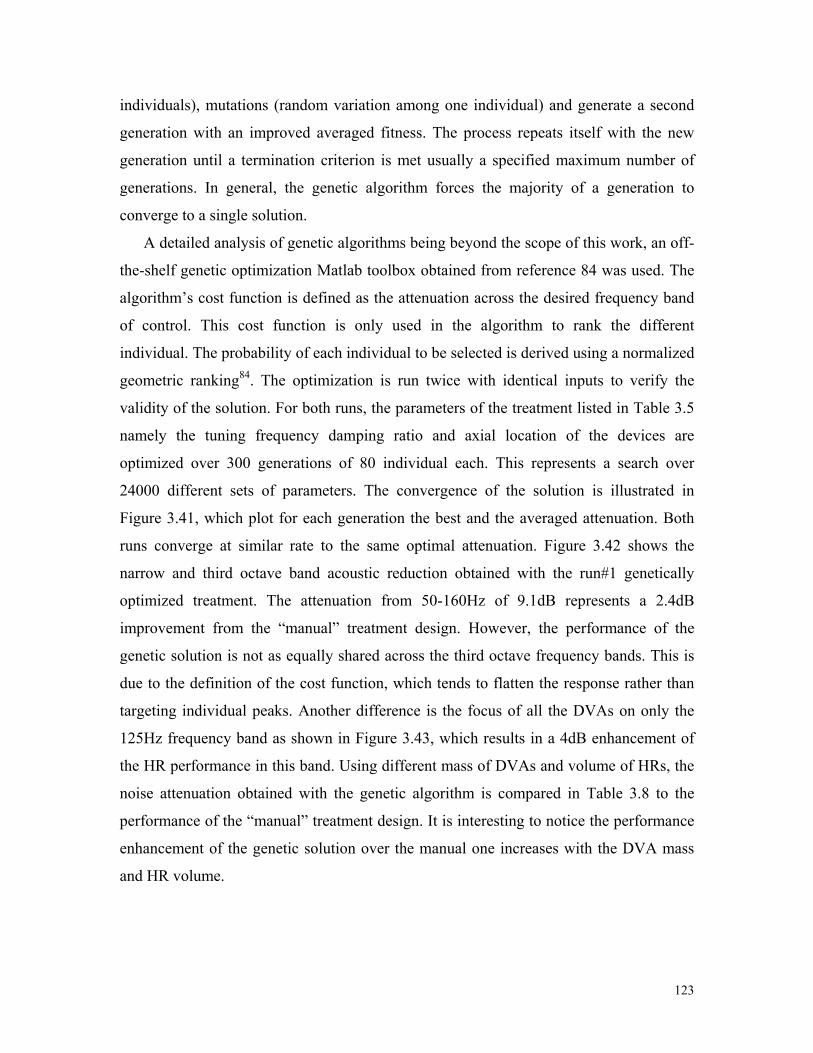
123
individuals), mutations (random variation among one individual) and generate a second
generation with an improved averaged fitness. The process repeats itself with the new
generation until a termination criterion is met usually a specified maximum number of
generations. In general, the genetic algorithm forces the majority of a generation to
converge to a single solution.
A detailed analysis of genetic algorithms being beyond the scope of this work, an off-
the-shelf genetic optimization Matlab toolbox obtained from reference 84 was used. The
algorithm’s cost function is defined as the attenuation across the desired frequency band
of control. This cost function is only used in the algorithm to rank the different
individual. The probability of each individual to be selected is derived using a normalized
geometric ranking84. The optimization is run twice with identical inputs to verify the
validity of the solution. For both runs, the parameters of the treatment listed in Table 3.5
namely the tuning frequency damping ratio and axial location of the devices are
optimized over 300 generations of 80 individual each. This represents a search over
24000 different sets of parameters. The convergence of the solution is illustrated in
Figure 3.41, which plot for each generation the best and the averaged attenuation. Both
runs converge at similar rate to the same optimal attenuation. Figure 3.42 shows the
narrow and third octave band acoustic reduction obtained with the run#1 genetically
optimized treatment. The attenuation from 50-160Hz of 9.1dB represents a 2.4dB
improvement from the “manual” treatment design. However, the performance of the
genetic solution is not as equally shared across the third octave frequency bands. This is
due to the definition of the cost function, which tends to flatten the response rather than
targeting individual peaks. Another difference is the focus of all the DVAs on only the
125Hz frequency band as shown in Figure 3.43, which results in a 4dB enhancement of
the HR performance in this band. Using different mass of DVAs and volume of HRs, the
noise attenuation obtained with the genetic algorithm is compared in Table 3.8 to the
performance of the “manual” treatment design. It is interesting to notice the performance
enhancement of the genetic solution over the manual one increases with the DVA mass
and HR volume.

124
Rings of 13 DVAs 4% of Mass=75Kg
Ring# Tuning
frequency (Hz)
Mass ratio (%)
Damping ratio (%)
Axial position
(m) 1 113/113.5 2 4.3/5.3 1.57/1.58 2 122/124 2 4.2/3.3 1.58/1.58
Rings of 7 HRs 5% of Volume=13m3
Ring# Tuning
frequency (Hz)
Volume ratio (%)
Damping ratio (%)
Axial position
(m) 1 84/86 1 10/7 2.74/2.75 2 115.6/117.6 1 15/10 2.73/2.72 3 142.6/149.6 1 8.6/7 1.54/1.63 4 144/154.6 1 10/18 0.03/0.0 5 146.7/156.6 1 7.7/9.3 2.71/2.75
Table 3.7 Parameters of the genetically optimized treatment for run#1 (in blue) and run#2
in red.
0 50 100 150 200 250 3002
4
6
8
10
Generation number
Atte
nuat
ion
in (d
B)
run#1
Best Averaged per generation (80 individuals)
0 50 100 150 200 250 3002
4
6
8
10run#2
Generation number
Atte
nuat
ion
in (d
B)
Best Averaged per generation (80 individuals)
Figure 3.41 Convergence of the genetic algorithm for run#1 and 2.

125
50 100 150 200-90
-85
-80
-75
-70
-65
-60
-55
-50A
cous
tic p
oten
tial e
nerg
y (d
B)
Frequency (Hz)
bare HR HR+DVA
63 80 100 125 1600
1
2
3
4
5
6
7
8
9
1/3 octave center frequency (Hz)A
cous
tic a
ttenu
atio
n (d
B)
HR HR+DVA
Figure 3.42 Narrow and third octave acoustic energy reduction for a genetically
optimized treatment.

126
50 100 150 200-80
-75
-70
-65
-60
-55K
inet
ic e
nerg
y (d
B)
Frequency (Hz)
bare DVA HR+DVA
63 80 100 125 160-2
-1
0
1
2
3
4
5
6
1/3 octave center frequency (Hz)V
ibra
tion
atte
nuat
ion
(dB
)
DVA HR+DVA
Figure 3.43 Narrow and third octave band vibration attenuation for the genetically
optimized treatment.
50-160Hz Attenuation (dB) Volume of HRs (% of cavity’s
volume)
Mass of DVA (% of cylinder’s
mass) “Manual” Genetic 2.5 2 5.0 6.8 5 4 6.7 9.1 10 8 9.1 12.2
Table 3.8 Performance comparison between the “manual” treatment in Table 3.5 and the
genetic algorithm solution for different mass of DVAs and volume of HRs.
To verify that the number of different tuning frequencies allowed in the treatment
does not limit the optimal performance, another optimization was done. In this case, the
treatment is composed of twice as many rings as in run#1 but with the same overall DVA
mass and HR volume. The convergence of the solution to 9.0 dB is illustrated in Figure
3.44 and the treatment parameters are listed in Table 3.9. Although a couple of HR rings

127
seems to be the duplicate of each other as rings 2 and 3 and rings 9 and 10, overall, the
tuning of the devices spread across the band. However, the axial position of the rings
corresponds consistently in every run to antinodes of the modes. It is interesting to notice
that the increase in possible tuning frequencies did not increase the performance of the
treatment for this cylinder within this frequency range.
0 50 100 150 200 250 3004
6
8
10
Generation number
Atte
nuat
ion
in (d
B)
Best Averaged per generation (80 individuals)
Figure 3.44 Convergence of the genetic algorithm for run#3.
Rings of 13 DVAs 4% of Mass=75Kg
Ring# Tuning
frequency (Hz)
Mass ratio (%)
Damping ratio (%)
Axial position
(m) 1 99.5 1 24.1 1.59 2 111.5 1 6.1 1.44 3 125.6 1 2.9 1.60 4 140.8 1 5.6 1.70
Rings of 7 HRs 5% of Volume=13m3
Ring# Tuning
frequency (Hz)
Volume ratio (%)
Damping ratio (%)
Axial position
(m) 1 86.0 0.5 9.0 2.74 2 102.3 0.5 17.1 2.74 3 109.0 0.5 18.4 2.74 4 116.3 0.5 17.4 2.74 5 118.6 0.5 5.0 1.45 6 138.8 0.5 4.4 1.58 7 145.0 0.5 12.7 2.73 8 152.8 0.5 8.4 0.02 9 156.8 0.5 8.9 2.68 10 159.7 0.5 6.5 2.71
Table 3.9 Parameters of the genetically optimized treatment for run#3.
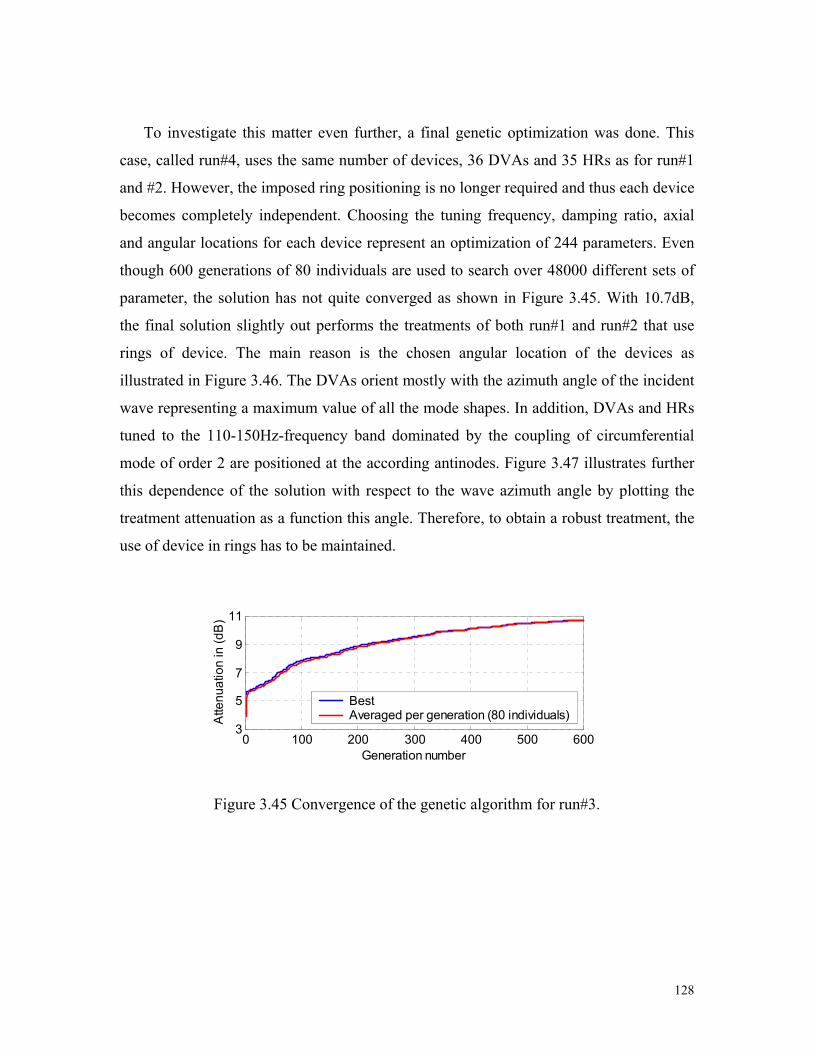
128
To investigate this matter even further, a final genetic optimization was done. This
case, called run#4, uses the same number of devices, 36 DVAs and 35 HRs as for run#1
and #2. However, the imposed ring positioning is no longer required and thus each device
becomes completely independent. Choosing the tuning frequency, damping ratio, axial
and angular locations for each device represent an optimization of 244 parameters. Even
though 600 generations of 80 individuals are used to search over 48000 different sets of
parameter, the solution has not quite converged as shown in Figure 3.45. With 10.7dB,
the final solution slightly out performs the treatments of both run#1 and run#2 that use
rings of device. The main reason is the chosen angular location of the devices as
illustrated in Figure 3.46. The DVAs orient mostly with the azimuth angle of the incident
wave representing a maximum value of all the mode shapes. In addition, DVAs and HRs
tuned to the 110-150Hz-frequency band dominated by the coupling of circumferential
mode of order 2 are positioned at the according antinodes. Figure 3.47 illustrates further
this dependence of the solution with respect to the wave azimuth angle by plotting the
treatment attenuation as a function this angle. Therefore, to obtain a robust treatment, the
use of device in rings has to be maintained.
0 100 200 300 400 500 6003
5
7
9
11
Generation number
Atte
nuat
ion
in (d
B)
Best Averaged per generation (80 individuals)
Figure 3.45 Convergence of the genetic algorithm for run#3.

129
DVA tuning frequency (Hz)80 100 120 140 160 180
-1 -0.5 0 0.5 1
-1
-0.5
0
0.5
1
x (m)
y (m
)
HR tuning frequency (Hz)80 100 120 140 160 180
-1 -0.5 0 0.5 1
-1
-0.5
0
0.5
1
x (m)
y (m
)
plane wave
plane wave
Figure 3.46 Position of the DVA and HR tuning frequencies around the cylinder
circumference for the genetic solution of run#4.
080
90
45135
-45-135
-90
10 dB
5 dB
0
Figure 3.47 Noise attenuation of the run#4 treatment as a function of the azimuth angle θi
of the incident wave.

130
3.4.3 Performance robustness to uncertainty in the excitation, system and
treatment
As illustrated with the genetic results presented previously, the solution to the optimal
noise reduction is not unique. Using rings of devices ensures the treatment will perform
identically regardless of the azimuth angle of the incident plane wave. To check the
treatment robustness to the elevation angle, the performance of the run#1 solution
genetically optimized for an angle of 70° is evaluated for other angles. The resulting
attenuation is then compared to the optimal performance achievable at each angle. Figure
3.48 illustrates these results and demonstrates the performance robustness of a combined
HR/DVA treatment to the elevation angle of the incident wave. For all angles ranging
from 25° to 85°, the treatment optimized form 70° remains within 1dB of the optimal
solution. This result is to be expected since the main mechanism of control is damping
and not modal restructuring which is more sensitive to changes in the primary excitation.
It was demonstrated in 3.4.1 that the effectiveness of a HR/DVA treatment depends
on the amount of damping initially present in the system. To evaluate the performance
sensitivity to another system variation, the treatment obtained in run#1 is evaluated with
the structural and acoustic natural frequencies of the cylinder perturbed. This perturbation
is obtained using a uniform random distribution constrained within a certain percentage
of the modes initial natural frequency. Averaging over 20 different systems with
permutations up to 20%, the treatment averaged attenuation decrease from 9.2dB to
8.0dB with a variance of 1.3dB. When reduced to perturbations of 10%, the performance
is almost unaffected with an averaged attenuation of 8.8dB of variance 0.2dB. These
results show the fairly good robustness of an HR/DVA treatment to random variations in
the system natural frequencies.
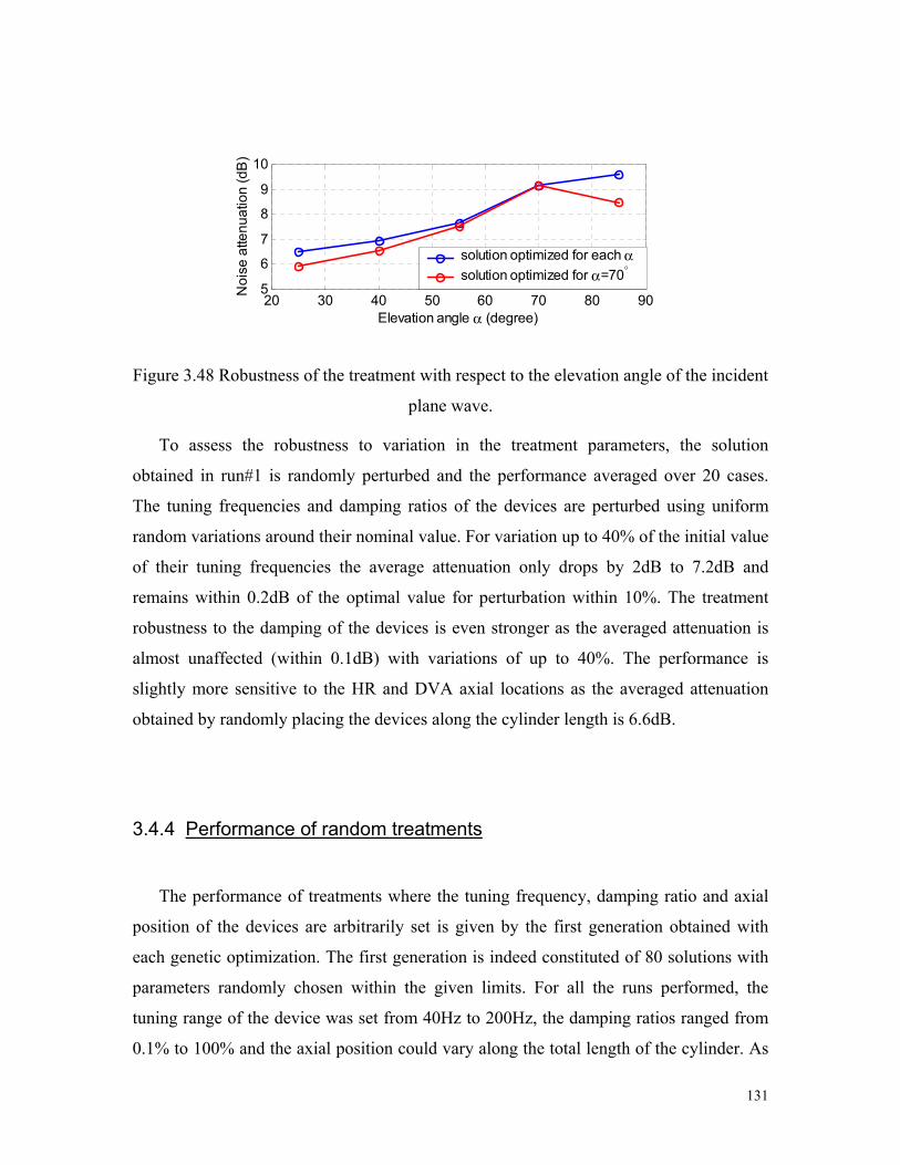
131
20 30 40 50 60 70 80 905
6
7
8
9
10
Elevation angle α (degree)
Noi
se a
ttenu
atio
n (d
B)
solution optimized for each α solution optimized for α=70°
Figure 3.48 Robustness of the treatment with respect to the elevation angle of the incident
plane wave.
To assess the robustness to variation in the treatment parameters, the solution
obtained in run#1 is randomly perturbed and the performance averaged over 20 cases.
The tuning frequencies and damping ratios of the devices are perturbed using uniform
random variations around their nominal value. For variation up to 40% of the initial value
of their tuning frequencies the average attenuation only drops by 2dB to 7.2dB and
remains within 0.2dB of the optimal value for perturbation within 10%. The treatment
robustness to the damping of the devices is even stronger as the averaged attenuation is
almost unaffected (within 0.1dB) with variations of up to 40%. The performance is
slightly more sensitive to the HR and DVA axial locations as the averaged attenuation
obtained by randomly placing the devices along the cylinder length is 6.6dB.
3.4.4 Performance of random treatments
The performance of treatments where the tuning frequency, damping ratio and axial
position of the devices are arbitrarily set is given by the first generation obtained with
each genetic optimization. The first generation is indeed constituted of 80 solutions with
parameters randomly chosen within the given limits. For all the runs performed, the
tuning range of the device was set from 40Hz to 200Hz, the damping ratios ranged from
0.1% to 100% and the axial position could vary along the total length of the cylinder. As

132
seen in Figure 3.41 and Figure 3.44, the averaged attenuation over these 80 random
solutions is around 3.5dB. Out of these 80 random treatments, the best one achieved an
attenuation of 5.5dB. This shows that with enough devices that at least equal the number
of the lightly damped resonances in the frequency band of control, a HR/DVA treatment
designed randomly might provide some attenuation. However, as Figure 3.41 and Figure
3.44 illustrate there is room for optimization. Treatments designed using some knowledge
of the system can indeed perform better than random ones while remaining quite robust
to changes in the excitation, the system or in treatment parameters.
3.5 Treatment design for the payload fairing
In this section the design process developed previously is applied to the much larger
real size fairing. Manually and genetically design treatment are discussed and the
performance and robustness are addressed.
3.5.1 The “manual” solution
Using a similar approach to the cylinder treatment design, the parameters are chosen
by examining the fairing response to the acoustic excitation described in section 3.2.5. In
the defined 30-90Hz frequency band of control, the number of dominating acoustic peaks
appearing in Figure 3.25 sets the number of HR rings to 8. The number of DVAs ring is
set to 4 each representing 1% of the fairing mass. The total volume of the HR treatment is
restricted to 2% of the fairing volume. The number of device per ring is 36 in order match
with the finite element mesh of the structure and acoustic cavity. To position each ring at
the modal antinodes, each dominating mode is visualized and identified using and
equivalent cylinder mode order. To avoid a concentration of the devices on one antinode
common to several modes, compromises are made to ensure a different axial position for
each rings. Using the approximate mode orders, the optimal damping ratios of the devices

133
are obtained using the derivation presented in section 3.3.1. Table 3.10 lists the
parameters of the resulting treatment.
Rings of 36 DVAs 4% of fairing mass
Targeted mode
Tuning frequency
(Hz)
Mass ratio (%)
Damping ratio (%)
Axial position
(m) (3,3) 52 1 7.0 2.0 (1,5) 56 1 7.0 3.9 (3,2) 78 1 7.0 7.0 (6,4) 93 1 7.0 10.0
Rings of 36 HRs 2% of fairing volume
Targeted mode
Tuning frequency
(Hz)
Volume ratio (%)
Damping ratio (%)
Axial position
(m) (0,1,0) 37 0.25 7 0.15 (1,1,0) 44 0.25 9 7.50 (2,1,0) 53 0.25 9 4.44 (0,2,0) 60 0.25 8 1.37 (3,1,0) 65 0.25 9 11.2 (1,2,0) 70 0.25 12 6.48 (2,2,0) 75 0.25 12 9.20 (3,2,0) 85 0.25 12 10.0
Table 3.10 Parameters of the “manual” treatment design.
Figure 3.49 shows the internal SPL in narrow and third octave band for the HR and
combined HR+DVA treatment. In the four third octave bands comprised within 30 and
90Hz, the acoustic attenuation exceeds 3dB. The HR treatment achieved reductions up to
10dB at the acoustic peaks, and the 100Hz third octave band although outside the band of
control presents some attenuation. The overall noise reduction in the 30-90Hz band
obtained with the HR treatment is 3.5dB. The DVA treatment improves this performance
to 3.9dB, which is equally spread across the band. The vibration attenuation illustrated in
Figure 3.50, shows the lower coupling level between the acoustic cavity and the structure
than for the cylinder, as the HRs do not significantly affect the vibration levels. This
lower level of coupling between the cavity and the structure is in part due to the surface
density of the fairing, which is more than twice the surface density of the cylinder.
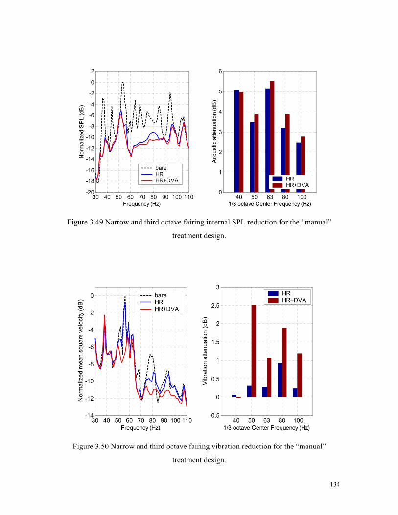
134
30 40 50 60 70 80 90 100 110-20
-18
-16
-14
-12
-10
-8
-6
-4
-2
0
2
Frequency (Hz)
Nor
mal
ized
SP
L (d
B)
bare HR HR+DVA
40 50 63 80 1000
1
2
3
4
5
6
Aco
ustic
atte
nuat
ion
(dB
)
1/3 octave Center Frequency (Hz)
HR HR+DVA
Figure 3.49 Narrow and third octave fairing internal SPL reduction for the “manual”
treatment design.
30 40 50 60 70 80 90 100 110-14
-12
-10
-8
-6
-4
-2
0
Frequency (Hz)
Nor
mal
ized
mea
n sq
uare
vel
ocity
(dB
)
bare HR HR+DVA
40 50 63 80 100-0.5
0
0.5
1
1.5
2
2.5
3
Vib
ratio
n at
tenu
atio
n (d
B)
1/3 octave Center Frequency (Hz)
HR HR+DVA
Figure 3.50 Narrow and third octave fairing vibration reduction for the “manual”
treatment design.
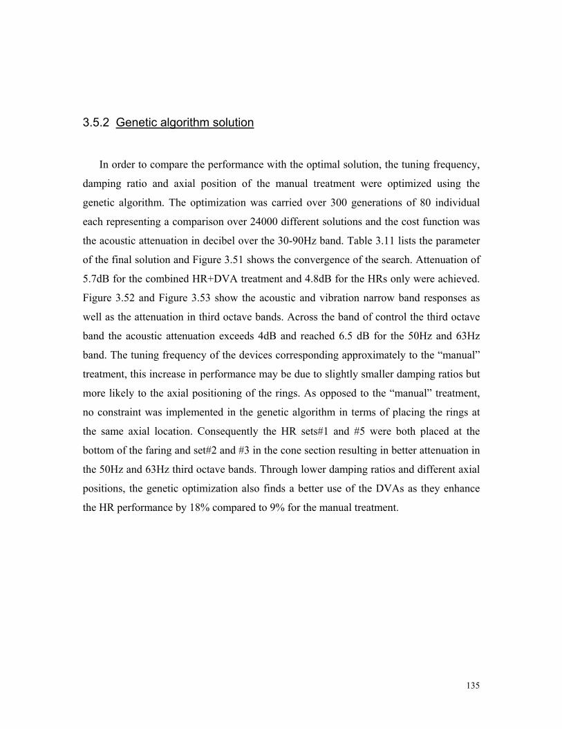
135
3.5.2 Genetic algorithm solution
In order to compare the performance with the optimal solution, the tuning frequency,
damping ratio and axial position of the manual treatment were optimized using the
genetic algorithm. The optimization was carried over 300 generations of 80 individual
each representing a comparison over 24000 different solutions and the cost function was
the acoustic attenuation in decibel over the 30-90Hz band. Table 3.11 lists the parameter
of the final solution and Figure 3.51 shows the convergence of the search. Attenuation of
5.7dB for the combined HR+DVA treatment and 4.8dB for the HRs only were achieved.
Figure 3.52 and Figure 3.53 show the acoustic and vibration narrow band responses as
well as the attenuation in third octave bands. Across the band of control the third octave
band the acoustic attenuation exceeds 4dB and reached 6.5 dB for the 50Hz and 63Hz
band. The tuning frequency of the devices corresponding approximately to the “manual”
treatment, this increase in performance may be due to slightly smaller damping ratios but
more likely to the axial positioning of the rings. As opposed to the “manual” treatment,
no constraint was implemented in the genetic algorithm in terms of placing the rings at
the same axial location. Consequently the HR sets#1 and #5 were both placed at the
bottom of the faring and set#2 and #3 in the cone section resulting in better attenuation in
the 50Hz and 63Hz third octave bands. Through lower damping ratios and different axial
positions, the genetic optimization also finds a better use of the DVAs as they enhance
the HR performance by 18% compared to 9% for the manual treatment.

136
Rings of 36 DVAs 4% of fairing mass
Set# Tuning
frequency (Hz)
Mass ratio (%)
Damping ratio (%)
Axial position
(m) 1 51.1 1 2.0 5.71 2 55.5 1 2.0 6.23 3 73.4 1 2.3 2.29 4 81.9 1 5.3 6.73
Rings of 36 HRs 2% of fairing volume
Set# Tuning
frequency (Hz)
Volume ratio (%)
Damping ratio (%)
Axial position
(m) 1 37.7 0.25 8.1 0.15 2 48.9 0.25 5.9 9.56 3 53.6 0.25 5.6 9.56 4 60.9 0.25 5.6 5.70 5 63.7 0.25 12.3 0.15 6 67.8 0.25 5.5 7.00 7 79.0 0.25 5.9 8.00 8 87.0 0.25 5.0 6.73
Table 3.11 Parameters of the genetically optimized treatment.
0 50 100 150 200 250 3002
3
4
5
6
Generation number
Atte
nuat
ion
in (d
B)
Best Averaged per generation (80 individuals)
Figure 3.51 Convergence of the genetic algorithm.
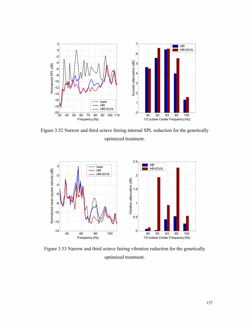
137
30 40 50 60 70 80 90 100 110-20
-18
-16
-14
-12
-10
-8
-6
-4
-2
0
2
Frequency (Hz)
Nor
mal
ized
SP
L (d
B)
bare HR HR+DVA
40 50 63 80 1000
1
2
3
4
5
6
7
Aco
ustic
atte
nuat
ion
(dB
)
1/3 octave Center Frequency (Hz)
HR HR+DVA
Figure 3.52 Narrow and third octave fairing internal SPL reduction for the genetically
optimized treatment.
40 60 80 100-14
-12
-10
-8
-6
-4
-2
0
Frequency (Hz)
Nor
mal
ized
mea
n sq
uare
vel
ocity
(dB
) bare HR HR+DVA
40 50 63 80 1000
0.5
1
1.5
2
2.5
Vib
ratio
n at
tenu
atio
n (d
B)
1/3 octave Center Frequency (Hz)
HR HR+DVA
Figure 3.53 Narrow and third octave fairing vibration reduction for the genetically
optimized treatment.

138
3.5.3 Performance robustness to variation in the excitation, system and
treatment.
To check the robustness of the genetic solution to changes in the disturbance speaker
locations, the performance of the treatment is evaluated for four different external fields.
Figure 3.54 shows the location of the speakers for the different cases and the resulting
attenuation provided by the treatment. Setup#1 corresponds to the initial configuration
used in the genetic optimization, which uses 12 monopoles. This particular configuration
was chosen to approximate the experimental setup detailed in section 4.4. Setup#3 and #4
represents slight variations around the nominal position, whereas setup#2 and setup#5 use
only 3 and 1 monopole respectively. The corresponding attenuation listed in Figure 3.54
shows the robustness of the treatment to changes in the acoustic external field.
To assess the sensitivity of the solution to variations in the system, the same method
used for the cylinder is applied. It consists in perturbing the structural and acoustic
natural frequencies of the fairing within a certain percentage of their initial value with a
uniform random distribution. To evaluate the robustness of the performance to treatment
variation, the tuning frequency and damping are also perturbed using this method.
Averaging over 20 instances. The reference unperturbed treatment is the genetically
obtained design which achieved acoustic attenuation of 5.7dB in the 30-90Hz band and
whose parameters are listed in Table 3.11. The acoustic attenuation resulting from
different level of variations for each case are detailed in Table 3.12. A first remark is that
the performance of the treatment is more sensitive to changes in the resonant frequencies
of the system than in the variation in devices’ tuning frequency. This is due to the
difference in the number of devices (288 HRs and 144 DVAs) and the number of
important acoustic and structural resonances (less than 20). When a resonance is shifted a
whole set of HRs or DVAs becomes detuned whereas the probability of having all the
devices targeting a specific mode detuned at the same time is very small. A second
remark is that as for the cylinder case, the performance sensibility to variation in the
devices’ damping ratio is very small. In addition to the aforementioned probabilistic
effect due to the very large number of devices, the amount of attenuation is a fairly weak
function of the device’s damping ratio as it was mentioned in section 3.3.1. Therefore,
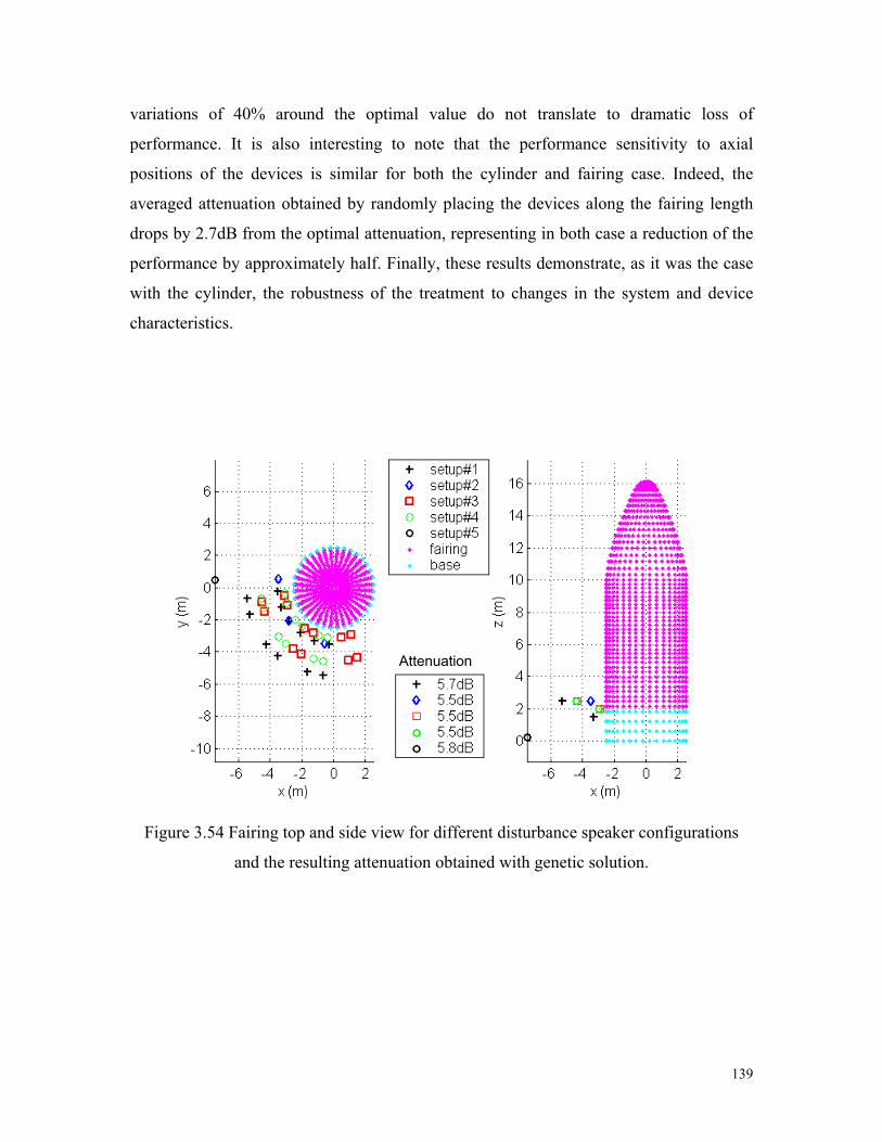
139
variations of 40% around the optimal value do not translate to dramatic loss of
performance. It is also interesting to note that the performance sensitivity to axial
positions of the devices is similar for both the cylinder and fairing case. Indeed, the
averaged attenuation obtained by randomly placing the devices along the fairing length
drops by 2.7dB from the optimal attenuation, representing in both case a reduction of the
performance by approximately half. Finally, these results demonstrate, as it was the case
with the cylinder, the robustness of the treatment to changes in the system and device
characteristics.
Figure 3.54 Fairing top and side view for different disturbance speaker configurations
and the resulting attenuation obtained with genetic solution.
Attenuation

140
Variable parameter Attenuation (dB) (Unperturbed: 5.7dB) System natural
frequencies Device tuning
frequency Device damping
ratio
±10% 4.9 5.5 5.6
±20% 4.4 5.1 5.6 V
aria
tion
±40% 3.6 4.4 5.6
Table 3.12 Performance robustness to changes in the system and treatment
characteristics.
3.5.4 Performance of random treatments
As for the cylinder, the results for the first generation of the genetic optimization are
used to illustrate how arbitrarily designed treatment perform. Figure 3.51 shows that 80
different treatments with random tuning, damping and axial positions yield an averaged
attenuation of 2.4dB. The best out of these 80 different solutions achieves an attenuation
of 3.5dB. The smaller difference in the performance between the random and the
optimized treatment obtained with the faring in comparison with the cylinder can be due
to a higher number of devices with respect to the number of dominant resonances in the
control band. However, as illustrated by Figure 3.51, some knowledge of the system can
lead to treatment that greatly outperform random ones. In addition, as demonstrated in the
previous paragraph, variation around the optimal treatment parameters to not reduced
drastically the performance.
3.6 Conclusions
In this chapter, the analytical model of the sound transmission into an enclosed
cylinder developed in Chapter 2 is validated experimentally. Using numerical simulations
the noise transmission mechanisms were analyzed for the cylinder and for the fairing
case. After the description of the noise control mechanisms of the DVA and HR, a

141
strategy for designing acoustic treatments with these structural and acoustic devices was
developed. The results obtained on both the cylinder and the fairing model, were
compared to the performance of treatments optimized with a genetic algorithm. Finally,
the robustness of the solutions with respect to variation in the excitation, system
characteristics, and in the devices parameters was addressed.
Using the cylinder model, the characteristics of the sound transmission through this
particular structure were highlighted. The behavior of this system, composed of two
resonant sub-systems namely the structure and the acoustic cavity, is dictated first by the
coupling of the disturbance acoustic field with the structure (external coupling) and
second by the coupling between the structure and the acoustic cavity (internal coupling).
The external coupling presents a filtering effect of the higher circumferential order
structural modes due to the mismatch of the wavenumber in the structure and in air. This
effect is stronger for axisymetric structures as spill over of the higher wave numbers only
occurs in their axial direction, as opposed to plates or curved panels, which present this
spill over in both directions. This filtering effect is important as it permits a reduction in
the number of modes necessary to describe the sound transmission.
The internal coupling is both spatial and frequency related. Spatially, it represents the
matching level between the structural and the acoustic modes of the cavity over the
surface of the cylinder, and is also particular to axisymetric system. Indeed, only modes
with equal circumferential orders and with axial orders in an even-odd (or odd-even)
combination will couple resulting in a sparse coupling matrix between the two modal
systems. However, experimentally, the acoustic transmission proved to be sensitive to
imperfections in the mode shapes and boundary conditions that couple all the modes
together. Consequently, a better sound transmission prediction was obtained when the
zeros of the sparse coupling matrix where replaced by small random numbers to simulate
this cross modal coupling. The level of internal coupling is also a function of the distance
between the natural frequencies of spatially coupled modes. Acoustic modes with higher
orders have higher natural frequency but for structural modes, because of the membrane
effect, this relationship between natural frequency and mode order is distorted. The first
acoustic modes are predominantly excited by structural modes with much higher natural
142
frequency resulting in a low frequency coupling. This situation was also observed in the
fairing. However, for the smaller and lighter cylinder, the noise transmission is
dominated by two spatially well-coupled modes with very close resonant frequencies. All
these coupling mechanisms are important for the selection of a modal subset that leads to
a good approximation of the system response with the minimum computation.
Finally, the damping of the structure and the acoustic cavity is an important parameter
to evaluate the treatment performance. As one source of structural damping comes from
energy loss by acoustic radiation, the effect of the fluid loading was implemented in both
models. It was found that because the cylinder is such a light structure, the surrounding
fluid add a lot of damping especially to the low circumferential order modes (up to 5%)
and can also lower their natural frequency by acting as an additional mass. Including this
commonly neglected effect helped to validate the model and allowed the performance of
the acoustic treatment to be accurately predicted.
The noise reduction mechanisms of the control devices were then presented. Based on
the principle of tuned-mass dampers, the damping of the HR and DVA can be optimized
for broadband attenuation. By applying a multitude of these small devices onto a large
system, sharp acoustic and structural resonance present in the frequency band of control
can be damped thus reducing sound transmission. DVAs and HRs were hence built and
applied to the cylinder in order to validate experimentally the model. For both the
structural and acoustic response, good agreement with the model was observed.
After validating the model, a procedure to designing an acoustic treatment composed
of both HRs and DVAs was then proposed and applied to both the cylinder and the
fairing. The strategy was to target each of the dominant resonances present in the acoustic
spectrum with the control devices. Each device was split into several units evenly
distributed around the circumference to be independent of the azimuth angle of the
disturbances and to avoid unfavorable modal interactions. The number of devices in each
ring depended on the circumferential order of the targeted mode. Starting with the
optimal solution derived in the literature for broadband control of a single mode, the
optimal damping ratios were then adapted to the ring positioning of the devices. The axial
location of the devices was chosen to correspond to an antinode of the targeted mode.

143
Fixing the mass of the DVAs and the volume of the HRs as these variable are directly
linked to the device effectiveness, the treatment performance (defined as the noise
attenuation in the control band) was then evaluated and compared to the optimal solution
obtained with a genetic algorithm. For the cylinder, the genetic solution presented a
2.4dB improvement over the 6.7dB attenuation obtained by the “manual” design across
the 50-160Hz band. However, the attenuation provided by the genetic solution was not
equally shared across the third octave bands due to the cost function that tend to flatten
the response. For the fairing, the genetic achieved a 2.2dB improvement over the
“manual” design 3.5dB attenuation from 30-90Hz. In this case, because no particular
band dominated the response, the manual and genetic performance were uniformly spread
across the third octave bands. As the noise reduction mechanisms are based on adding
damping to sharp resonances, the amount of damping initially present in the system
greatly affects the performance of a treatment. Simulations showed the performance
variation of the “manual” cylinder treatment as a function of the initial structural and
acoustic damping ratios. It showed that for ratios below 3% the HR and DVA can
provided significant noise attenuation, above 6dB.
Finally the robustness of the treatment to changes in the excitation characteristics, in
the system natural frequencies, in the tuning frequency, damping ratio and axial location
of the devices was addressed for both the cylinder and the fairing. For both systems, the
performance proved to be robust to any combination of changes but particularly to the
damping ratio of the devices. This robustness is inherent of the noise reduction
mechanism, which is based on adding damping to lightly damped resonances of the
system. Therefore, as long as the initial system is lightly damped the treatment will
perform well. Due to the large number of devices applied to the system, the performance
of random treatments i.e. where the axial locations, tuning frequencies and damping
ratios of the devices are set arbitrarily within limits was investigated. It was showed that
even if on average a random treatment can provide up to 3.5dB of attenuation, the
proposed design procedure based on some knowledge of the system, can greatly out
perform these random treatments. In addition, this optimal solution does not lie in a steep
narrow valley of the cost function surface, and therefore was proved to be robust.

144
Chapter 4 Outdoor high level tests
4.1 Introduction
This chapter describes the two series of tests conducted at Virginia Tech on the
Boeing cylinder and the final test conducted at the Boeing facilities in California on a
launch vehicle fairing.
The objective of the cylinder tests was to demonstrate the performance of HR/DVA
treatment under realistic launch conditions. As a consequence the experiments took place
outdoors at the Virginia Tech airport as it provided the space and isolation necessary to
conduct such loud and large-scale experiments. The disturbance noise level reached
130dB.
The first test in 2001, involved the empty cylinder, whereas in the second one in
2002, the cylinder was partially filled with a mock payload. The treatment, designed
using the developed numerical code, was adjusted using preliminary experiments.
The objective of the fairing test organized in collaboration with the Boeing team, was
to assess the performance of a pre-flight treatment. Prototypes of the noise reduction
devices were designed at Virginia Tech under strict flight constraints, and then mass-
produced and incorporated in the launch vehicle fairing by Boeing designers.
4.2 Empty cylinder test November 14th-30th, 2001
This section covers the outdoor test done on the empty cylinder under high-level
acoustic excitation.

145
4.2.1. Test setup
The cylinder transported to the outdoor test site was craned onto a 2.5 ft wood base
and rolled under a large tent as shown in Picture 4.1.
Picture 4.1 Cylinder being craned onto the base and then placed under the large tent at the
outdoor test site.
A large speaker system was hired and set up on one side of the cylinder. The speaker
system consisted of eight enclosures each with four 18 inch 400 watt drivers totaling a
12.8 Kilowatts capability. The speaker system was designed to work in the 40-250Hz
range. The power amplification and measurement equipment was housed in a trailer
placed next to the tent and the electrical power supplied by a generator (see Picture 4.2).

146
Picture 4.2 Test site showing the tent, equipment trailer and the power generator
As seen in Picture 4.3, the cylinder was instrumented with a ring of 30 accelerometers
evenly spaced 40 inches up the cylinder and a line of 5 accelerometers running the length
of the cylinder and facing the speaker array. Outside the cylinder 6 B&K microphones
monitored the acoustic field exciting the cylinder. A set of 16 PCB microphones were
placed on a tree inside the cylinder and rotated to measure a total of 32 interior positions.
The top end cap was also instrumented with 4 accelerometers to measure the vibration
and to assess the potential flanking (i.e unwanted sound transmission through the end
cap). Figure 4.1 is a schematic showing all of the instrumentation positions and speaker
positions used for this test.
tent trailer
generator
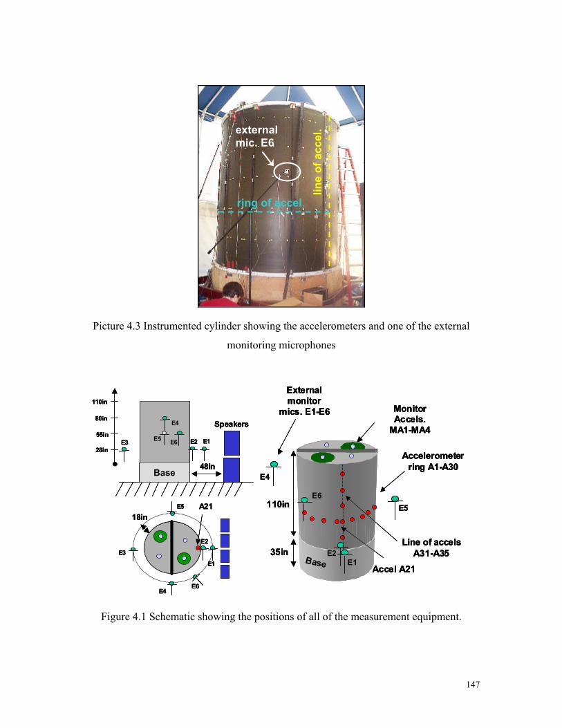
147
Picture 4.3 Instrumented cylinder showing the accelerometers and one of the external
monitoring microphones
Base
E1E2E3
E4
E6E5
Speakers
48in
28in
55in
80in
110in
E1
E2
E3
E4E6
E5 A2118in
Accelerometer ring A1-A30
Line of accelsA31-A35
External monitor
mics. E1-E6 Monitor Accels.
MA1-MA4
Accel A21Base
110in
35in E2E1
E4
E6E5
Base
E1E2E3
E4
E6E5
Speakers
48in
28in
55in
80in
110in
Base
E1E2E3
E4
E6E5
Speakers
48in
28in
55in
80in
110in
E1
E2
E3
E4E6
E5 A2118in
E1
E2
E3
E4E6
E5 A2118in
Accelerometer ring A1-A30
Line of accelsA31-A35
External monitor
mics. E1-E6 Monitor Accels.
MA1-MA4
Accel A21Base
110in
35in E2E1
E4
E6E5
Accelerometer ring A1-A30
Line of accelsA31-A35
External monitor
mics. E1-E6 Monitor Accels.
MA1-MA4
Accel A21Base
110in
35in E2E1
E4
E6E5
Figure 4.1 Schematic showing the positions of all of the measurement equipment.
external mic. E6
ring of accel.
line
of a
ccel
.
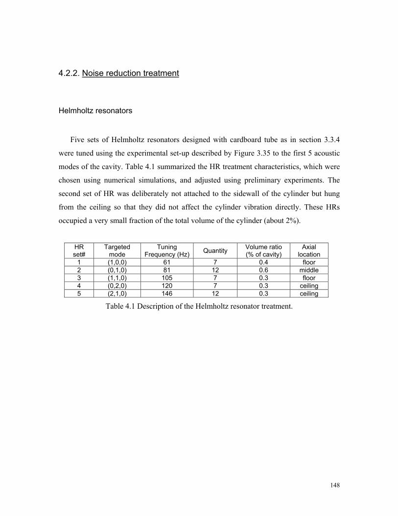
148
4.2.2. Noise reduction treatment
Helmholtz resonators
Five sets of Helmholtz resonators designed with cardboard tube as in section 3.3.4
were tuned using the experimental set-up described by Figure 3.35 to the first 5 acoustic
modes of the cavity. Table 4.1 summarized the HR treatment characteristics, which were
chosen using numerical simulations, and adjusted using preliminary experiments. The
second set of HR was deliberately not attached to the sidewall of the cylinder but hung
from the ceiling so that they did not affect the cylinder vibration directly. These HRs
occupied a very small fraction of the total volume of the cylinder (about 2%).
HR set#
Targeted mode
Tuning Frequency (Hz) Quantity Volume ratio
(% of cavity) Axial
location 1 (1,0,0) 61 7 0.4 floor 2 (0,1,0) 81 12 0.6 middle 3 (1,1,0) 105 7 0.3 floor 4 (0,2,0) 120 7 0.3 ceiling 5 (2,1,0) 146 12 0.3 ceiling
Table 4.1 Description of the Helmholtz resonator treatment.

149
Picture 4.4 View looking down in the cylinder with the HR treatment.
Distributed vibration absorbers
The DVA treatment consisted in three rings of 15 devices. Each DVA has a 3inch by
5inch footprint and were tuned to 72Hz, 95Hz and 145Hz corresponding to the (1,3),
(2,3) and (1,2) structural modes. Representing 3, 2.5, and 1% of the cylinder’s mass
respectively, the 3 rings were placed around the midpoint as shown in Figure 4.2.
72Hz
95Hz145Hz
55inch
00 2403360
72Hz
95Hz145Hz
55inch
00 2403360
0 0 240336 0 0 0 240336 0
Figure 4.2 DVAs spaced every 240 and around the midpoint up the cylinder
mic. tree
HR
foam

150
4.2.3. Results
Acoustic forcing characterization
The external coupling between an incident plane and the structural modes of the
cylinder was discussed in section 3.2.1. In order to characterize this external coupling in
the experiment configuration, the transfer function between the speakers signal, 40-
250Hz band-passed white noise, and microphones situated at the surface of the cylinder
were measured. Seven rings of 12 microphones evenly space along the length of the
cylinder meshed the pressure distribution. Assuming the structural mode shapes, a spatial
Fourier transform can determine the structural modal component of the incident acoustic
field. Due to the limited number of measurement in the axial (7) and circumferential (12)
direction, the spatial Fourier transform is only valid that is with minimum aliasing, up to
ns=3 and ms=6. Figure 4.3 shows a contour plot of these modal components for four
different frequencies. Although, the speaker acoustic field differs from a theoretical plane
wave, due in particular to the reflection from the ground, the main characteristic of the
external coupling remains similar. Only the low circumferential order (ms<4) are well
excited up to 180Hz. The variation with the axial order is harder to analyze partly due to
the under sampling. In this direction, the acoustic field differs more from a plane wave
excitation, since the pressure decays along the cylinder axis as Figure 4.4 illustrates.
However, this particularity of the field might be closer to a real launch acoustic
environment.
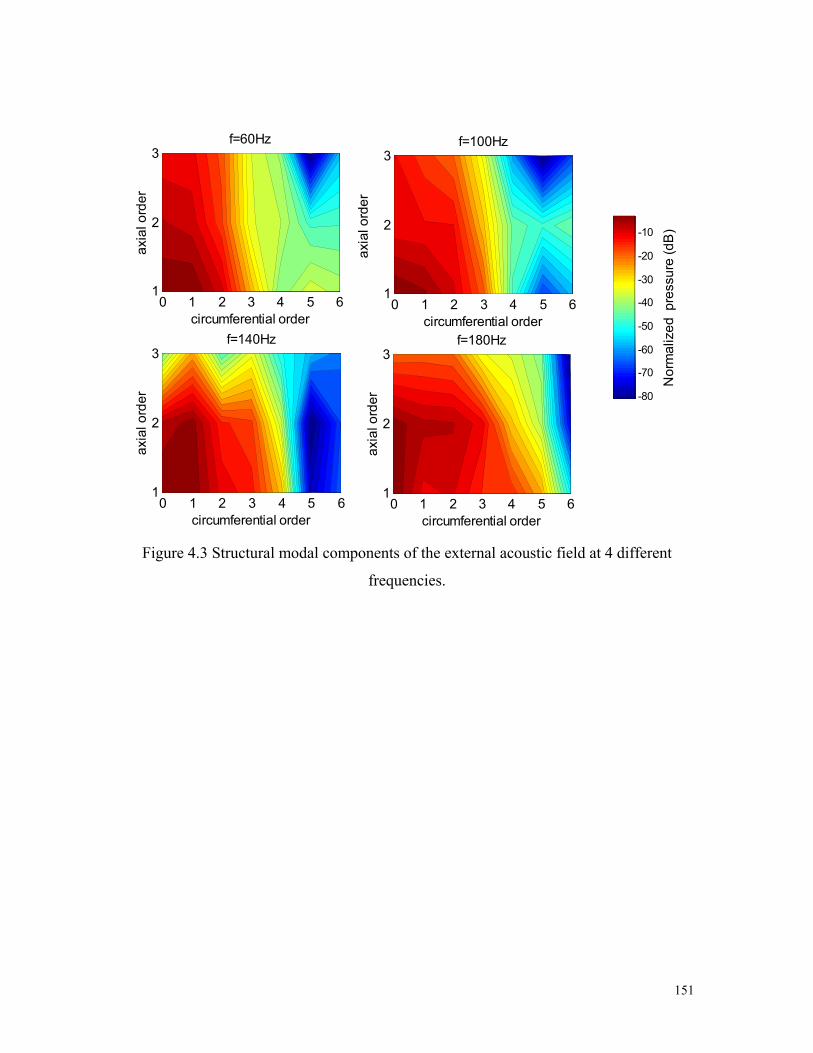
151
0 1 2 3 4 5 61
2
3ax
ial o
rder
circumferential order
f=180Hz
0 1 2 3 4 5 61
2
3
axia
l ord
er
circumferential order
f=140Hz
0 1 2 3 4 5 61
2
3
axia
l ord
er
circumferential order
f=100Hz
Nor
mal
ized
pre
ssur
e (d
B)
-80
-70
-60
-50
-40
-30
-20
-10
0 1 2 3 4 5 61
2
3ax
ial o
rder
circumferential order
f=60Hz
Figure 4.3 Structural modal components of the external acoustic field at 4 different
frequencies.

152
Nor
mal
ized
ext
erna
l pre
ssur
e (d
B)
-20
-18
-16
-14
-12
-10
-8
-6
-4
-2
40 60 80 100 120 140 160 180
0.5
1
1.5
2
Frequency (Hz)
Axi
al p
ositi
on o
n cy
linde
r (m
)
Figure 4.4 Variation of the external pressure distribution along the length of the cylinder
as a function of frequency.
Bare baseline
The performance of the different treatments is compared in this paragraph to the non-
treated cylinder that is with “bare” walls. Since the measurement were taken over a
number of days, the external microphones ensure that changes in interior acoustic levels
were not due to changes in the primary field. Figure 4.17 shows the consistency (within
0.5dB) of the external acoustic level measured at microphone E#2 (see Figure 4.1) for the
three different configurations.

153
40 60 80 100 120 140 160 180100
105
110
115
Frequency (Hz)
Ext
erna
l SP
L at
mic
.2 (d
B re
f 2 ×1
0 -5
)bare HR HR+DVA
50 63 80 100 125 160 100
101
102
103
104
105
106
107
108
109
110
111
Ext
erna
l SP
L at
mic
.2 (d
B re
f 2 ×1
0 -5
)1/3 octave Center Frequency (Hz)
bare HR HR+DVA
Figure 4.5 Narrow and third octave band external SPL for the three different
configurations.
Using the ring of accelerometers, a spatial Fourier transform is performed to identify
the modal content of the cylinder’s vibration. As shown in Figure 4.6, the velocity of the
structure is dominated across the band by higher order circumferential modes
(m=7,8,9,10). This is contradictory with the circumferential filtering characteristic of the
external coupling illustrated by Figure 4.3. The imperfection in the boundary conditions
at the end-caps and the circumferential discontinuities induced by the seven sheets
composing the cylinder skin can be responsible for the inter-structural modal coupling
pointed out by the arrows in Figure 4.6. As a consequence the vibration response of the
cylinder becomes hard to predict, as the orthogonal trigonometric assumption of the
mode shapes seems violated experimentally.
The performance of the DVA and HR+DVA treatment on the velocity response
averaged over the 35 accelerometers is illustrated in Figure 4.7. In addition to their
targeted mode at 75, 95 and 145Hz, the DVAs attenuate greatly all the lightly damped
peaks from 50 to 120Hz. Since the (1,2) structural mode is barely excited by the external
acoustic field, the measure velocity response is relatively different than the response

154
predicted by the model. Indeed, the predicted response was only composed of coupled of
well-excited modes and was dominated especially by the interaction between the 1,2
structural mode and 0,2,0 acoustic mode in the 120Hz range. As a consequence, the HRs
do not enhance the vibration reduction provided by the DVAs as it was observed in
section 3.4.1. Furthermore, the (0,2,0) acoustic mode at 121 Hz predominantly coupled to
the (1,2) structural mode, was therefore unexcited and hence did not appear in the interior
acoustic spectrum. Consequently, the fourth set of resonator was removed from the
treatment.
Figure 4.6 Normalized velocity wavenumber transform applied on the ring of
accelerometers.
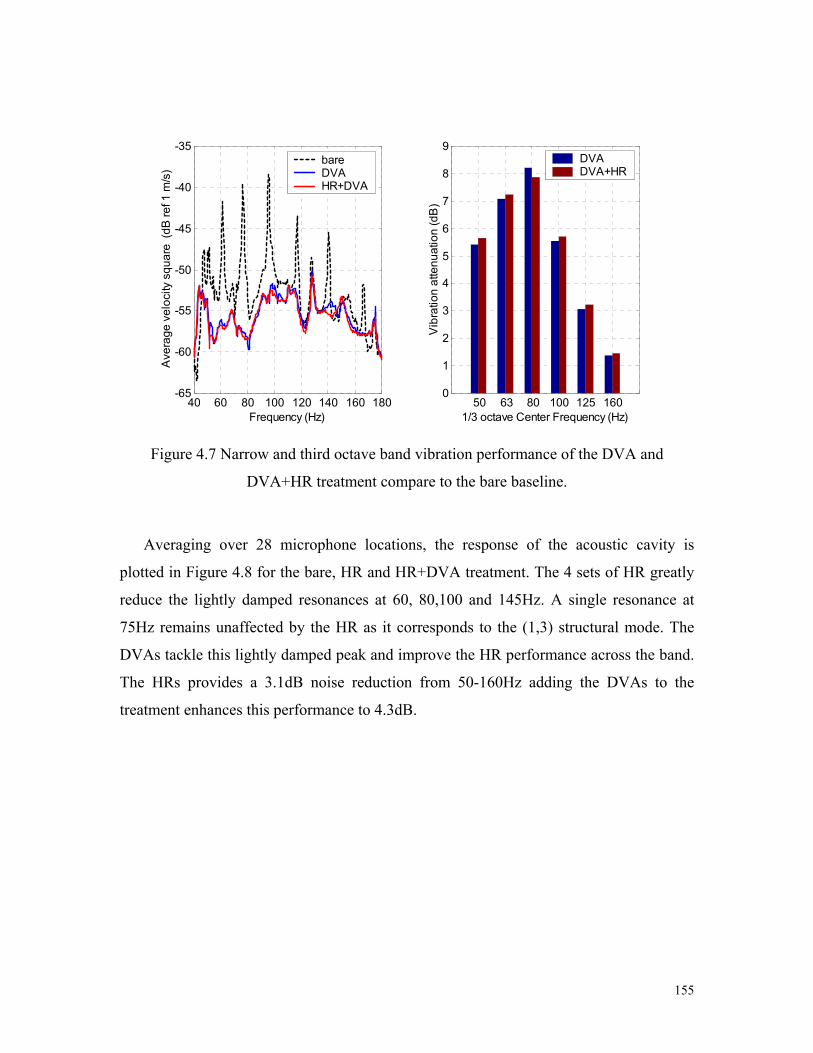
155
40 60 80 100 120 140 160 180-65
-60
-55
-50
-45
-40
-35
Frequency (Hz)
bare DVA HR+DVA
50 63 80 100 125 160 0
1
2
3
4
5
6
7
8
9
Vib
ratio
n at
tenu
atio
n (d
B)
1/3 octave Center Frequency (Hz)
DVA DVA+HR
Ave
rage
vel
ocity
squ
are
(dB
ref 1
m/s
)
Figure 4.7 Narrow and third octave band vibration performance of the DVA and
DVA+HR treatment compare to the bare baseline.
Averaging over 28 microphone locations, the response of the acoustic cavity is
plotted in Figure 4.8 for the bare, HR and HR+DVA treatment. The 4 sets of HR greatly
reduce the lightly damped resonances at 60, 80,100 and 145Hz. A single resonance at
75Hz remains unaffected by the HR as it corresponds to the (1,3) structural mode. The
DVAs tackle this lightly damped peak and improve the HR performance across the band.
The HRs provides a 3.1dB noise reduction from 50-160Hz adding the DVAs to the
treatment enhances this performance to 4.3dB.

156
40 60 80 100 120 140 160 18075
80
85
90
95
100
105
Frequency (Hz)
Inte
rnal
SP
L (d
B re
f 2x1
0 -5)
bare HR HR+DVA
50 63 80 100 125 160 0
1
2
3
4
5
6
7
Aco
ustic
atte
nuat
ion
(dB
)
1/3 octave Center Frequency (Hz)
HR HR+DVA
Figure 4.8 Narrow and third octave band acoustic performance of the HR and HR+DVA
treatments compare to the bare baseline.
Half foam baseline
In an effort to make the cylinder behave as close as a real fairing as possible, a second
baseline was used. It consisted in covering part of the cylinder’s interior wall with some
acoustic foam such that the level of acoustic damping approaches the one observed in
fairings. This was achieved by matching reverberation time measurements and is detailed
in Appendix A. The resulting baseline, called half-foam is composed of 2inch-thick
melamine foam covering approximately half of the cylinder’s wall surface.
Figure 4.9 presents, using the same scale as in Figure 4.7, the vibration response for
the HR and combined HR+DVA treatment compared to the half foam baseline. The
vibration level achieved by the combined HR+DVA treatment remains similar than when
used with bare walls. Because the foam provides some damping to the initially lightly
damped structural modes especially at the higher frequencies, the treatment performance
in third octave bands is reduced compared to the bare foam baseline. Nevertheless, from
50 to 120Hz, the vibration attenuation exceeds 3dB in each band.

157
40 60 80 100 120 140 160 180-65
-60
-55
-50
-45
-40
-35
Frequency (Hz)
Ave
rage
vel
ocity
squ
are
(dB
ref 1
m/s
) half foam half foam+HR half foam+HR+DVA
50 63 80 100 125 160 -1
0
1
2
3
4
5
Vib
ratio
n at
tenu
atio
n (d
B)
1/3 octave Center Frequency (Hz)
HR HR+DVA
Figure 4.9 Narrow and third octave band vibration performance of the HR and HR+DVA
treatments compare to the half foam baseline.
The acoustic response of the cavity presented in Figure 4.10 (also using same scale as
Figure 4.8) illustrates the damping effect of the foam in the higher frequencies. The
145Hz resonance is for instance reduced by 15dB. The acoustic levels obtained with the
combined HR+DVA treatment remain similar to one obtained with the bare baseline. The
performance of the treatments reduces especially in the 160Hz third octave band. From
50Hz to 110Hz, the HR provides 2.2dB noise attenuation, which is enhanced to 3.3dB by
the DVAs.
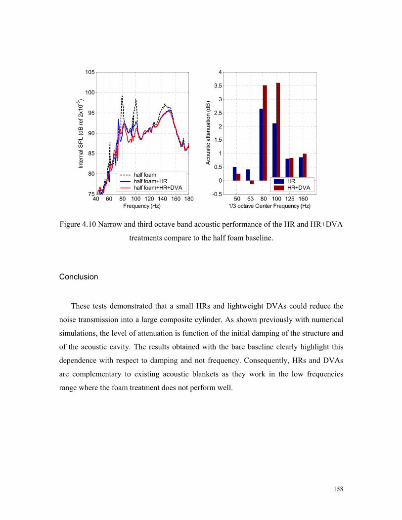
158
40 60 80 100 120 140 160 18075
80
85
90
95
100
105
Frequency (Hz)
Inte
rnal
SP
L (d
B re
f 2x1
0 -5)
half foam half foam+HR half foam+HR+DVA
50 63 80 100 125 160 -0.5
0
0.5
1
1.5
2
2.5
3
3.5
4
Aco
ustic
atte
nuat
ion
(dB
)1/3 octave Center Frequency (Hz)
HR HR+DVA
Figure 4.10 Narrow and third octave band acoustic performance of the HR and HR+DVA
treatments compare to the half foam baseline.
Conclusion
These tests demonstrated that a small HRs and lightweight DVAs could reduce the
noise transmission into a large composite cylinder. As shown previously with numerical
simulations, the level of attenuation is function of the initial damping of the structure and
of the acoustic cavity. The results obtained with the bare baseline clearly highlight this
dependence with respect to damping and not frequency. Consequently, HRs and DVAs
are complementary to existing acoustic blankets as they work in the low frequencies
range where the foam treatment does not perform well.

159
4.3 Partially filled cylinder test October 2002
This section describes the outdoor tests done on the partially filled cylinder under
high-level acoustic excitation.
4.3.1 Test setup
As for the empty cylinder test of October 2001, the cylinder was housed under a
30’x30’x16’ tent at the Virginia Tech airport. The data acquisition equipment was also
secured in a trailer. A 60KW Watt generator was used to power all the equipment used
during testing and positioned 100’ away from the test setup. The cylinder was excited by
a total of 16 bass speakers equipped with horn loaded 15” driver and this time placed on
each side of cylinder as shown in Figure 4.11.
Payload
Cylinder
Speakers
Amplifiers
TrailerData Acquisition Equipment
Tent (30’ x 30’x16’)
Payload
Cylinder
Speakers
Amplifiers
TrailerData Acquisition Equipment
Tent (30’ x 30’x16’)
Payload
Cylinder
Speakers
Amplifiers
TrailerData Acquisition Equipment
Tent (30’ x 30’x16’)
Figure 4.11: Cylinder inside the tent and experiment layout diagram.
speaker
speaker

160
One of the focuses of this test was to characterize the effectiveness of the treatment
when the cylinder’s cavity is partially filled with a mock payload. The mock payload
provided by Boeing is a 6’ diameter, 7’ tall cylinder with a wooden frame, wooden end-
caps, and an aluminum-sheet shell. The interior is lined with 3” melamine foam to damp
any acoustic and structural resonances. A crane truck was rented for the period of the test,
as it was necessary to remove the payload from the cylinder in order to work on the
different acoustic treatment as shown in Picture 4.5.
Picture 4.5 Craning operation of the mock payload from the cylinder
For these tests, 15 internal microphones were flush mounted to the payload, a ring of
30 and a line of 7 accelerometers monitored the cylinder’s vibration, and 4 external
microphones monitored the external SPL. The two walls of speakers were driven with
two independent white noise band passed between 40 and 400Hz. The time histories of
the two inputs as well as all the sensors were recorded and post-processed using Matlab.
end-cap plug
Mock payload

161
4.3.2 Noise reduction treatment
Partially filled acoustic cavity natural frequencies
In order to design a Helmholtz resonator treatment, the natural frequencies of the
partially filled cylinder cavity needed to be identified. The mock payload being shorter
than the cylinder, the cavity resonant frequencies could not be accurately predicted using
the theoretical annular cavity equation derived in section 2.3.1. Therefore, Boeing
provided the natural frequencies and mode shapes of the partially filled cavity obtained
with a finite element (FE) model as shown in Figure 4.12. In order to check these results,
and quantify the effect of the foam, a low-level acoustic transmission test as described in
Figure 4.13, was conducted. The acoustic disturbance was created by a 18” Yamaha
subwoofer, the transfer function between a line of 8 microphones positioned at the
payload surface and the white noise input to the speaker was acquired for 8 different
angles θ. The average of the square of the 64 transfer functions is plotted in Figure 4.14.
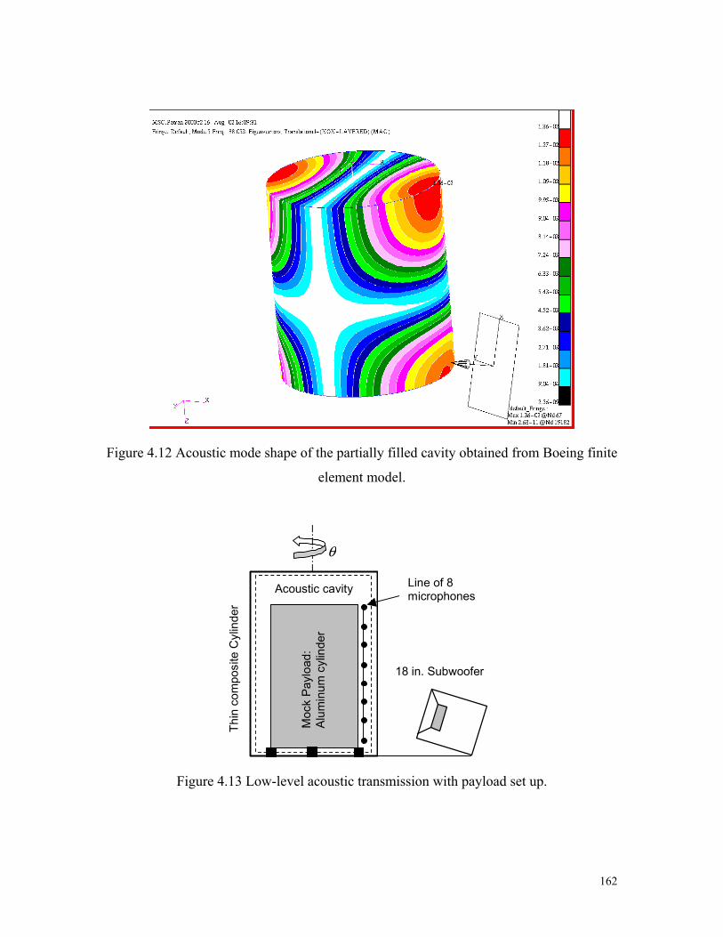
162
Figure 4.12 Acoustic mode shape of the partially filled cavity obtained from Boeing finite
element model.
Acoustic cavity
Thin
com
posi
te C
ylin
der
θ
Moc
k Pa
yloa
d:
Alu
min
um c
ylin
der
18 in. Subwoofer
Line of 8 microphones
Figure 4.13 Low-level acoustic transmission with payload set up.

163
40 60 80 100 120 140 160 180 20010
12
14
16
18
20
22
24
26
28
30
Frequency (Hz)
mea
n sq
uare
mic
. tra
nsfe
r fun
ctio
n (d
B)
Figure 4.14: mean square pressure transfer functions (64 microphones)
Because of the asymmetry of the acoustic cavity the mode shape extraction as
explained in section 3.2.4 is not as accurate as with the empty symmetric cavity.
However, the dominant acoustic modes could be identified and their natural frequencies
for the bare and half foam covered cavity are compared with the FE model in Table 4.2.
As the cavity remains axisymetric, the mode shape can be described using a
circumferential order. Although the axial nodal lines are slightly shifted compared to a
perfectly annular cavity, the axial order is retained to describe the mode shape. The
discrepancies between the FE and the experimental results may be due to the small
difference in the position of the payload, 4” from the cylinder bottom in the FE and 7.5”
in the experiment.

164
Resonant frequency (Hz) Mode order (n,m,p) FE Bare experimental Half foam experimental
(1,0,0) 48.9 52.5 57.5 (0,1,0) 60.2 62 60.5 (1,1,0) 88.0 87.5 85 (2,0,0) 102.6 99.5 98 (2,1,0) 129.2 128.5 127 (1,2,0) 132.6 127 125 (2,2,0) 163.9 162 145
Table 4.2 Resonant frequencies of the cavity filled with the mock payload
Helmholtz resonators
Using the same design strategy as for the empty cylinder tests, 6 sets of Helmholtz
resonators were designed and tuned to the frequencies of the cavity with half foam wall
coverage. The characteristics of this treatment are listed in Table 4.3 and Picture 4.6
shows the first 5 sets of HRs as well as the half foam treatment attached to the cylinder.
HR set#
Targeted mode
Tuning Frequency (Hz) Quantity Volume ratio
(% of cavity) Axial
location 1 (1,0,0) 57.5 4 1.1 floor 2 (0,1,0) 60.5 4 1.0 floor 3 (1,1,0) 85 12 1.5 ceiling 4 (2,0,0) 98 12 1.1 payload top 5 (1,2,0) 125 18 (6+12) 1.2 floor+ceiling 6 (2,2,0) 144 15 0.7 middle
Table 4.3 Description of the Helmholtz resonator treatment.

165
Picture 4.6 Five different HR (left). Half foam treatment (right).
The 6th set of resonators was designed as a hybrid HR/DVA. The idea is that the HR
mass could be used as the mass layer in a distributed vibration absorber. By varying the
foam thickness underneath the HR, the natural frequency of the resulting vibration
absorber could be varied. Figure 4.15 shows the HR/DVA used in this test with its
bouncing mode response measured using the experimental set up described in Figure
3.31. It is mainly this bouncing mode that couples into the structural vibration. Therefore,
this device targets the acoustic mode at 144Hz while simultaneously adds damping to the
(1,3) structural mode around 75Hz. Consequently, this set of HR could not be separated
from the DVA treatment. As for the previous tests, the first 5 sets of HRs were
deliberately not attached to the cylinder’s wall to prevent any mass loading effect on the
structural vibration. The HR volume ratios quoted in Table 4.3 are with respect to the
partially filled cavity, which with 5.7m3 represents 44% of the empty cylinder volume.
Therefore, the HRs only occupy 2.8% of the empty cylinder volume.
4’
57 H
z
60 H
z
85 H
z
98 H
z
125
Hz

166
40 60 80 100 120
-5
0
5
10
15
20
Frequency (Hz)
Mag
nitu
de (d
B)
Figure 4.15 HR/DVA and its bouncing natural frequency curve.
Distributed vibration absorbers
The DVA treatment consists of 2 rings of 15 DVAs. The first ring tuned to the (1,3)
structural mode at 74Hz is constituted of the HR/DVAs each weighing 400g. The second
ring tuned to 145Hz is constituted of 3” by 5” footprint DVA made of melamine foam
and a 60g aluminum plate. Picture 4.7 shows the two DVA rings position around the
midpoint of the cylinder. The total mass of the treatment was 7 Kg representing
approximately 9% of the cylinder’s mass.
HR throat
fd=75Hz ςd=6%
HR
foam spring
10”

167
Picture 4.7 HR/DVAs and DVAs spaced every 24° around the mid point up the cylinder
4.3.3 Results
Acoustic forcing characterization
The two walls of speakers being symmetrically position around the cylinder and
driven with two independent white noises, the incident acoustic field is only
characterized for one side. As for the previous test the transfer function between the
speakers signal and microphones at the cylinder surface are measured. This time, the
pressure distribution is meshed with 7 axial and 30 angular positions. Figure 4.16
highlights the main characteristics of the external acoustic field. With a higher spatial
sampling than with the previous test, the wavenumber transform shows that, below
180Hz, the external acoustic field excites only the lower circumferential order modes.
The wavenumber transform in the axial direction does not bring any interesting
information. However the pressure axial variation illustrates the amplitude decays from
the bottom to the cylinder top by approximately 15dB.

168
dB-16
-14
-12
-10
-8
-6
-4
-2
0.5 1 1.5 240
60
80
100
120
140
160
Fre
quen
cy (H
z)
Axial position on cylinder (m)
Normalized external pressure
dB
-50
-45
-40
-35
-30
-25
-20
-15
-10
-5
0 1 2 3 4 5 6 7 8 9 1040
60
80
100
120
140
160
Freq
uenc
y (H
z)Circumferential order
External pressure circumferential component
Figure 4.16 Characteristics of the external acoustic field created on the cylinder by one
side of speaker.
Treatment performance
As the different tests took place over several days, two microphones in front of each
speaker wall (mic#1 and #3), were consistently position 5” away from the cylinder
surface to monitor the external disturbance levels. The sound system was different than
with the previous tests, and the control of the level was not as easy. Therefore, all the
tests had to be scaled to one particular run using the two monitoring microphones. Figure
4.17 shows the narrow and third octave band of averaged over mic#1 and #3 for the three
different runs. An overall SPL of 132.5dB constituting a satisfactory approximation of
real launch conditions was achieved and the level difference between the runs in each
third octave band always remains within 1dB.

169
40 60 80 100 120 140 160 180104
106
108
110
112
114
116
Frequency (Hz)
Ext
enal
SP
L (d
B re
f 2 ×1
0 -5
)
half foam overall:132.5 dBHR overall:132.5 dB HR+DVA overall:132.5 dB
50 63 80 100 125 160 100
102
104
106
108
110
112
114
Ext
enal
SP
L (d
B re
f 2 ×1
0 -5
)1/3 octave Center Frequency
half foamHR HR+DVA
Figure 4.17 Narrow and third octave external SPL averaged between mic#1 and mic#3.
For this particular test, the performance of the HR and combined HR+DVA treatment
were compared only to a half-foam baseline, which consist of a 50% coverage of the
cylinder walls with 2inch thick melamine acoustic foam as shown in Picture 4.7.
Although the mock payload does no add any acoustic damping directly, by reducing the
volume of the cavity, it increase the effectiveness of the half foam treatment. As this
effect is also likely to occurs in the real application the 50% coverage is maintained as the
baseline to which the HR/DVA treatment is compared. As seen in Figure 4.18, the DVA
treatment leads to large vibration attenuation below 100Hz where lightly damped modes
resonate. This fairly high attenuation is to be expected as the DVAs represent about 9%
of the cylinder mass. The 145Hz-targeted resonance being already quite damped by the
foam blankets, the corresponding DVAs could be removed from the treatment without
affecting the performance and would reduce the treatment mass by 15%.
The acoustic performance is illustrated in Figure 4.19. Due to the rearrangement of
the acoustic mode due to the presence of the mock payload, the lightly damped
resonances dominating the acoustic spectrum appears at 60 and 80Hz as opposed to 80
and 100Hz for the empty cavity case (see Figure 4.10). These lightly damped peaks

170
below 100Hz are well tackled by the HRs. In the first three lower third octave band, the
DVAs enhance the HR attenuations by reducing the structural resonances well coupled to
the acoustic cavity such as the 75Hz 1,3 mode. These attenuation improvements are up to
2.5dB. As the acoustic modes above 100Hz are already damped by the foam treatment
the HRs performance in those frequency bands is undermined.
50 100 150-70
-65
-60
-55
-50
-45
-40
-35
Frequency (Hz)
Ave
rage
vel
ocity
squ
are
(dB
ref 1
m/s
)
half foam half foam+HR half foam+HR+DVA
50 63 80 100 125 160 -1
0
1
2
3
4
5
6
7
8
9
Vib
ratio
n at
tenu
atio
n (d
B)
1/3 octave Center Frequency (Hz)
HR HR+DVA
Figure 4.18 Narrow and third octave band vibration performance of the HR and
combined HR+DVA treatment compared to the half foam baseline.

171
40 60 80 100 120 140 160 18085
90
95
100
105
110
Frequency (Hz)
Inte
rnal
SP
L (d
B re
f 2 ×1
0-5)
half foam half foam+HR half foam+HR+DVA
50 63 80 100 125 160 -1
0
1
2
3
4
5
6
7
Aco
ustic
atte
nuat
ion
(dB
)
1/3 octave Center Frequency (Hz)
HR HR+DVA
Figure 4.19 Narrow and third octave band acoustic performance of the HR and HR+DVA
treatments compared to the half foam baseline.
Conclusion
These tests confirmed the conclusions drawn from the results obtained for the empty
cavity. The rearrangement of the acoustic modes induced by the mock payload led to
more structural acoustic coupling in the low frequency range. This allowed a clearer
demonstration of the DVAs role in noise reduction. This test also showed the feasibility
of hybrid HR/DVA that makes effective use of the HR mass to reduced noise
transmission. This issue is important in the long run as the overall mass of the treatment
will include the mass of the HR casing. The hybrid HR/DVA can be one solution to
reduce this overall mass.
172
4.4 Fairing test November-December 2003
This section describes the test conducted on a full-scale fairing at the Boeing facilities
in Huntington Beach CA. The design processes that lead to a pre-flight HR/DVA noise
reduction treatment is detailed. Then, the experimental set up and the results are
presented.
4.4.1 Lightweight Helmholtz resonator design
The design of a HR treatment for a full-size faring differs from the approach used
with the scaled cylinder prototype. The volume of the fairing being 16 times larger than
the cylinder prototype, a treatment representing a couple of percent of this volume
translates automatically into a very large number of resonators. In addition, Boeing
designers’ will to integrate the HRs to the pre-existing acoustic blanket treatment gives
the treatment a very high weight penalty. As a consequence, the feasibility of lightweight
HR was investigated.
The effect of wall elasticity on the effectiveness of a Helmholtz resonator motivated
by underwater applications has been subject to a couple of studies85,86. Both studies
conclude the wall compliance decreases the HR effective stiffness reducing its frequency
in comparison with an identically shaped rigid cavity by 1 2γ . This factor is a function of
the shell impedance Zs and the impedance of the fluid Zf and is given by
s
s f
ZZ Z
γ =+
, (4.4.1)
Photiadis85 shows that when the internal dissipation produced by viscosity and heat
conduction exceeds the radiation loss in air, which is mostly the case47,48, the damping
ratio of the elastic HR is increased. In addition, he also demonstrates that the resonator
net volume outflow is reduced by 2γ . As a consequence, the design of lightweight
efficient HR is based on the trade-off between the mass and the stiffness of the resonator

173
shell. After a spherical HR, not suited for this application, a cylindrical HR with
hemispherical end-cap presents the second stiffest type of cavity for a given material. In
collaboration with Boeing designers, a compromise between cost and effectiveness was
reached in using off the shelf plastic tube enclosed with regular slightly curved end-cap.
As the HR were to be embedded in the foam blankets the opening had to be placed on
the side of the tube rather than on the end-cap. To conserve symmetry and avoid quarter
wavelength tube behavior, the opening was placed in the middle of the tube section. The
type of plastic used is called PETG (for polyethyleneterephthalateglycolate) and presents
a density of 1270Kg/m3, the inner diameter of the tube is 5” as for the cardboard HR, and
its thickness is 0.025”. The 5” diameter was the maximum dimension intruding in the
payload bay, which was allowed by Boeing. The plastic end-caps are identical than the
one used for the cardboard HR, and the necks were made of acrylic tubes of different
diameter and length.
In order to verify the effectiveness of a PETG HR in the configuration of the test, a
foam bed consisting in a rectangular wood box filled with 3.5” thick foam was built. As
shown in Picture 4.8, a cardboard and a PETG HR of identical dimensions, 48” long with
a 1.5” diameter and 2” long neck, were tested in the foam bed using the experimental
setup described in Figure 3.35.
Picture 4.8 Cardboard and PETG HR in the test foam bed.
Cardboard HR (1.6 Kg)
Speaker
Foam bed
Speaker
Foam bed
PETG HR (0.47 Kg)
HR opening

174
The transfer function between the internal and external microphone is shown in
Figure 4.20 for both HRs. In agreement with the theory, the PETG HR presents a lower
natural frequency at 48Hz than the cardboard HR, assumed infinitely stiff, at 51Hz. The
amplitude at resonance, proportional to the HR net outflow, reduces from 9 to 7. It is
interesting to note that quantitatively these results agreed with Photiadis85:
248 7 0.88
51 9γ =
.
Note that this agreement is to take with caution as small error on the evaluated resonant
frequencies can lead to quite large variations in γ . The damping ratio is also increased
for the elastic HR. This experiment illustrates the previously mentioned trade-off. The
PETG HR, approximately 20% less effective, represent a 70% weight reduction
compared cardboard HR. This compromise was retained for the fairing test.
30 34 38 42 46 50 54 58 62 66 7010
0
101
Frequency (Hz)
|pin
t/pex
t|
Cardboard fh=51Hz ζh=6%PETG fh=48Hz ζh=8%
Figure 4.20 Transfer function between internal and external pressure obtained with the
cardboard and PETG HR.

175
A lot of the PETG tube presented permanent oval deformation yielding large
reduction of their stiffness and therefore HR performance. To overcome this problem,
stiffeners made out of plastic end-caps were inserted on each side of the neck to maintain
the circular cross section of the tube as shown in Picture 4.9. Due to the four large holes,
the stiffeners are acoustically invisible below 100Hz and thus do not alter the HR
behavior. The gain in performance is illustrated in Figure 4.21, which shows the transfer
function between the internal and external pressure for a PETG HR with and without
stiffeners. In the first case, it can be clearly seen that the shell dynamics impair the HR
resonance, whereas with the stiffen HR these dynamics occur outside the band, resulting
in a sharper acoustic resonance.
Picture 4.9 PETG HR with stiffeners.
Stiffener
Neck
End-cap

176
30 40 50 60 70 80 90 100 110 120-10
0
10
20
Frequency (Hz)
|FR
F| (d
B)
without stiffenerwith stiffener
30 40 50 60 70 80 90 100 110 120
-150
-100
-50
0
Frequency (Hz)
Pha
se (d
egre
e)
without stiffenerwith stiffener
Figure 4.21 Transfer function of a PETG HR with and without stiffener.
Placing acoustic foam in the HR opening to adjust the damping to the desired value
was no longer possible in the fairing application as the payload environment had be
cleared of any dust and particles. Consequently, the damping was created by covering the
HR opening with metal wire mesh of different percentage open area. Picture 4.10 shows
and example of 30% open wire mesh covering the HR neck.
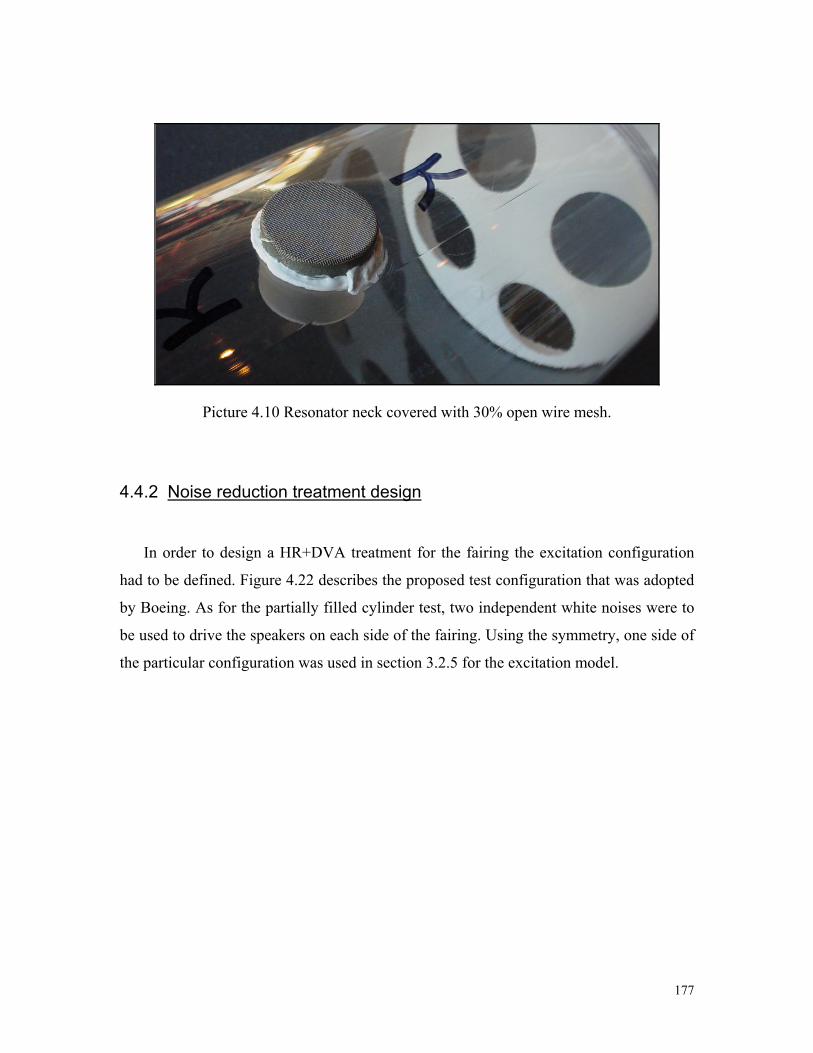
177
Picture 4.10 Resonator neck covered with 30% open wire mesh.
4.4.2 Noise reduction treatment design
In order to design a HR+DVA treatment for the fairing the excitation configuration
had to be defined. Figure 4.22 describes the proposed test configuration that was adopted
by Boeing. As for the partially filled cylinder test, two independent white noises were to
be used to drive the speakers on each side of the fairing. Using the symmetry, one side of
the particular configuration was used in section 3.2.5 for the excitation model.

178
2m (6.5 ft)
high speakerbass speaker
sideview
topview
white noise 2
white noise 1
side view
top view
20°20°
2m (6.5 ft) 2m (6.5 ft)
high speakerbass speaker
sideview
topview
high speakerbass speaker
sideview
topview
white noise 2
white noise 1
side view
top view
20°20°20°20°
Figure 4.22 Speaker layout for the payload fairing test.
The existing cell division of the fairing blanket, dictated the positioning of the HR
and DVA. In the cylindrical section, the 30”by 80” rectangular cells could only host 2
HRs and one DVA. To maximize their volume, two 40” long HR were placed in all the
cylinder cells. The DVA positioning was also constrained to the top or bottom of a cell.
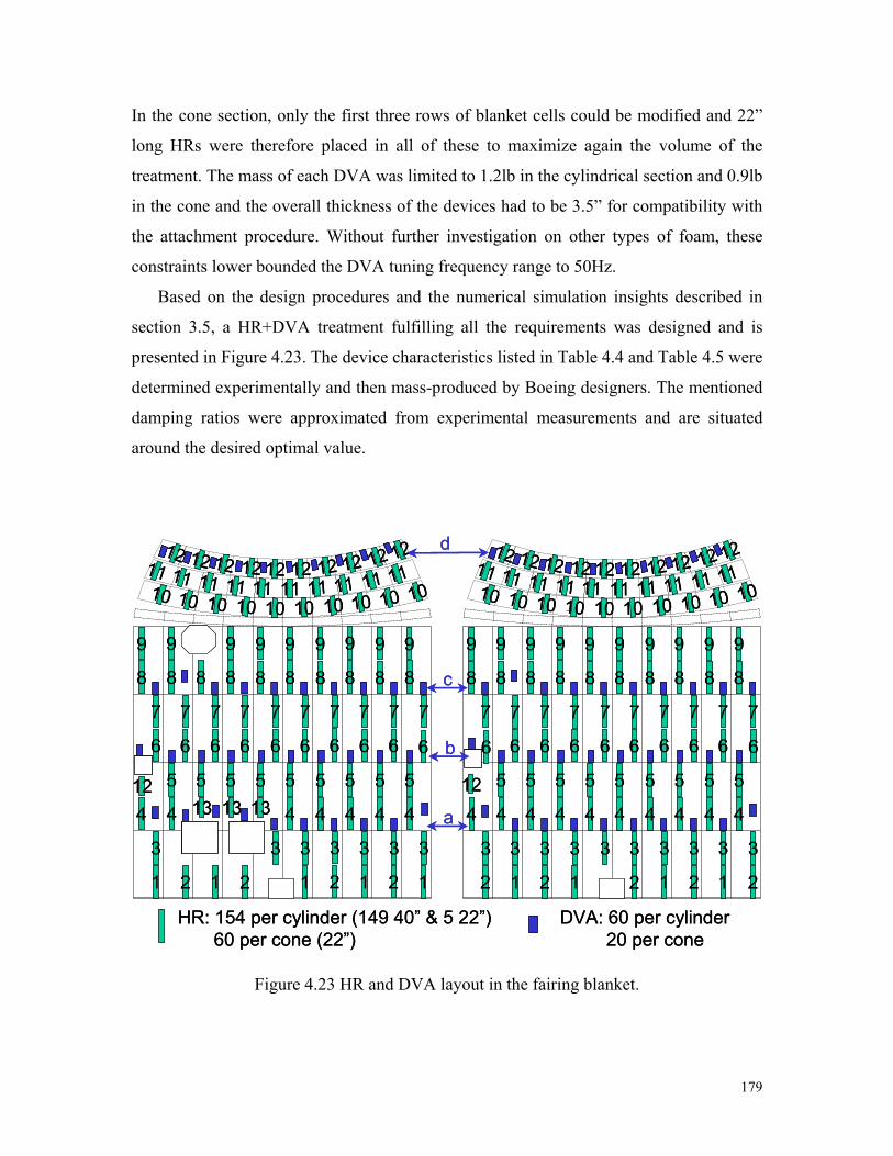
179
In the cone section, only the first three rows of blanket cells could be modified and 22”
long HRs were therefore placed in all of these to maximize again the volume of the
treatment. The mass of each DVA was limited to 1.2lb in the cylindrical section and 0.9lb
in the cone and the overall thickness of the devices had to be 3.5” for compatibility with
the attachment procedure. Without further investigation on other types of foam, these
constraints lower bounded the DVA tuning frequency range to 50Hz.
Based on the design procedures and the numerical simulation insights described in
section 3.5, a HR+DVA treatment fulfilling all the requirements was designed and is
presented in Figure 4.23. The device characteristics listed in Table 4.4 and Table 4.5 were
determined experimentally and then mass-produced by Boeing designers. The mentioned
damping ratios were approximated from experimental measurements and are situated
around the desired optimal value.
DVA: 60 per cylinder20 per cone
HR: 154 per cylinder (149 40” & 5 22”)60 per cone (22”)
101010101010 10 10 1010
111111111111 11 11 11
11
9
8
9
88
9
8
9
8
9
8
9
88
9
8
9
8
7
6
7
6
7
6
7
6
7
6
7
6
7
6
7
6
7
6
7
3
1 2 1 2
3 3
1
3
2
3
1
3
2
3
1
12121212121212121212
5
4
5
4
5
4
5
4
5
4
5555
44
101010101010 10 10 1010
111111111111 11 11 11
11
9
8
9
8
9
8
9
8
9
8
9
8
9
8
9
8
9
8
9
8
7
6
7
6
7
6
7
6
7
6
7
6
7
6
7
6
7
6
7
3
2
3
1
3
2
3
1
3 3
2
3
1
3
2
3
1
3
2
12121212121212121212
5
4
5
4
5
4
5
4
5
4
5
4
5
4
5
4
5
44
6 6
12 121313 13
9
a
b
c
d
Figure 4.23 HR and DVA layout in the fairing blanket.

180
40 inch long HR, 440g (149 units)
Set# Frequency (Hz)
Damping ratio (%)
Opening ID (in.)
Neck (in) Quantity % of fairing
volume 1 37 9.5 1 2-3/8 9 0.05 2 61 11 1-1/2 1-1/2 9 0.05 3 43 12 1 1-1/2 17 0.1 4 52 7 1-1/2 2-1/2 17 0.1 5 85 8 2 7/8 18 0.11 6 54 9 1-1/2 2-1/8 20 0.12 7 63 13 1-1/2 1-3/8 20 0.12 8 65 7.4 1-1/2 1-1/4 20 0.12 9 70 13 2 2 19 0.11
22 inch long HR, 260g (63 units) 10 71 12 1 7/8 20 0.07 11 75 12 1-1/2 2-3/8 20 0.07 12 85 7 1-1/2 2-3/8 20 0.07 13 52 12 1 2-1/4 3 0.01
Table 4.4 HR parameters of the launch vehicle treatment
1.2lb (545g) DVA (20 units per set)
Set# Frequency (Hz)
Damping ratio (%)
Foam thickness (in)
Aluminum plate thickness (in)
Footprint (in2)
% of fairing mass
a 56.3 2 3-1/8 .375 32 0.7 b 49.7 2 3 .50 24 0.7 c 74.5 2 3-1/2 .188 63-3/4 0.7
0.9lb (409g) DVA (20 units per set) d 91.4 3 3-1/2 .125 72 0.5
Table 4.5 DVA parameters of the launch vehicle treatment
The 41Kg overall mass of the 80 DVAs, represents 2.2% of the mass of the fairing
with its blanket. With 82Kg the 212 HRs adds 4.5% mass and represents 1.1% of the
fairing volume. Figure 4.24 shows the narrow and third octave band performance of this
particular treatment predicted using the model. As it will be considered in the
experiments, the 31.5Hz third octave band is included. However in the simulation, this
band only contain the tail of the first acoustic mode as it ranges from 28Hz to 35Hz. The
expected overall acoustic attenuation from 30-90Hz is of 3.2dB out of which 3.0dB is
obtained with the HRs only.

181
30 40 50 60 70 80 90 100 110-20
-18
-16
-14
-12
-10
-8
-6
-4
-2
0
2
Frequency (Hz)
Nor
mal
ized
SP
L (d
B)
bare HR HR&DVA
31.5 40 50 63 80 100 -2
-1
0
1
2
3
4
5
Aco
ustic
atte
nuat
ion
(dB
)
1/3 octave Center Frequency (Hz)
HR HR&DVA
Figure 4.24 Prediction of the acoustic performance of the treatment tested in the fairing.
4.4.3 Experimental setup
The tests took place inside a large building at the Boeing facilities in Huntington
Beach California. The fairing, and the speakers on their stands are shown in Picture 4.11.
In addition to the HR and DVA treatment, these tests were the opportunity for Boeing to
evaluate the performance of a new type of blanket. Unfortunately for cost reason, only
two noise treatments could be evaluated. The first corresponds to the existing acoustic
blanket made of 4.5-inch thick melamine foam and was conducted in October 2003 and is
called “bare”. The second corresponds to the new blanket composed of 3-inch thick
melamine foam and 0.5-inch thick polyamide foam, with the HRs and DVAs. As a
consequence, the contribution of each device to the acoustic reduction could not be
determined experimentally. The new acoustic blanket is however supposed to differ from
the existing blanket above 110Hz. The performance of the combined HR+DVA treatment
designed to work in the low frequencies would therefore be considered independent from
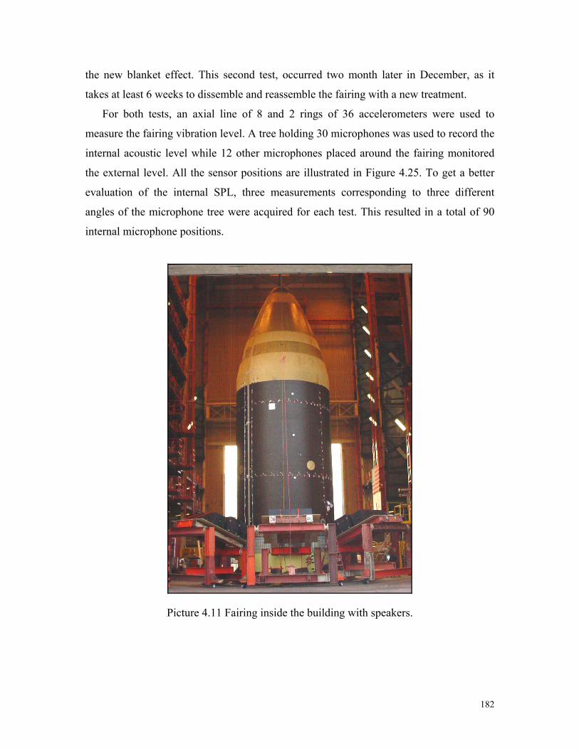
182
the new blanket effect. This second test, occurred two month later in December, as it
takes at least 6 weeks to dissemble and reassemble the fairing with a new treatment.
For both tests, an axial line of 8 and 2 rings of 36 accelerometers were used to
measure the fairing vibration level. A tree holding 30 microphones was used to record the
internal acoustic level while 12 other microphones placed around the fairing monitored
the external level. All the sensor positions are illustrated in Figure 4.25. To get a better
evaluation of the internal SPL, three measurements corresponding to three different
angles of the microphone tree were acquired for each test. This resulted in a total of 90
internal microphone positions.
Picture 4.11 Fairing inside the building with speakers.

183
2m (6.5ft)
12
10
4
1
9
57
11
8
3
2
6
1,4,10,12
2,3,6,8,11
9,5
7
accelerometerexternalmicrophone
internalmicrophone
37-72
1-36
73-80
1-10
11-20
21-30
2m (6.5ft)2m (6.5ft)
12
10
4
1
9
57
11
8
3
2
6
1,4,10,12
2,3,6,8,11
9,5
7
accelerometeraccelerometerexternalmicrophone
internalmicrophone
37-72
1-36
73-80
1-10
11-20
21-30
Figure 4.25 Location of the accelerometers and microphones for the fairing test.
4.4.4 Results.
The two tests being spaced by two months, the external SPL averaged over the 12
microphones was slightly higher for the second (HR+DVA) test as shown in Figure 4.26.
Therefore, for each frequency, the microphone and accelerometer signals of the second
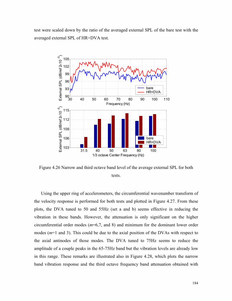
184
test were scaled down by the ratio of the averaged external SPL of the bare test with the
averaged external SPL of HR+DVA test.
30 40 50 60 70 80 90 100 11090
93
96
99
102
105
Frequency (Hz)
Ext
erna
l SP
L (d
B/re
f 2×1
0 -5
)
bare HR+DVA
31.5 40 50 63 80 100 103
106
109
112
115
1/3 octave Center Frequency (Hz)
Ext
erna
l SP
L (d
B/re
f 2×1
0 -5
)
bare HR+DVA
Figure 4.26 Narrow and third octave band level of the average external SPL for both
tests.
Using the upper ring of accelerometers, the circumferential wavenumber transform of
the velocity response is performed for both tests and plotted in Figure 4.27. From these
plots, the DVA tuned to 50 and 55Hz (set a and b) seems effective in reducing the
vibration in these bands. However, the attenuation is only significant on the higher
circumferential order modes (m=6,7, and 8) and minimum for the dominant lower order
modes (m=1 and 3). This could be due to the axial position of the DVAs with respect to
the axial antinodes of those modes. The DVA tuned to 75Hz seems to reduce the
amplitude of a couple peaks in the 65-75Hz band but the vibration levels are already low
in this range. These remarks are illustrated also in Figure 4.28, which plots the narrow
band vibration response and the third octave frequency band attenuation obtained with

185
the treatment. The difference of performance compared to the results obtained on the
cylinder illustrated in Figure 4.18, are mainly due to the difference in the mass ratio of
the DVAs. Indeed in this experiment, the DVA treatment represents only 2.2% of the
fairing mass whereas in the partially filled cylinder test, the DVAs represented 9% of the
cylinder mass. Furthermore, the effect of the last set of DVA (set d) tuned to 90Hz are
imperceptible as no resonance seemed to occurs in this band and the devices only
represent 0.5% of the fairing mass. The 3dB vibration increase in the 31.5Hz third octave
band (28-35Hz) is to take with caution as the speaker system can lack consistency in this
low range. In addition, the consistency in assembling the two fairing halves can affect the
structural dynamics in this low frequency range.
Figure 4.27 Circumferential wavenumber transform of the velocity response of the upper
ring for both treatments.
DVA effect

186
Figure 4.28 Narrow and third octave vibration performance of the fairing treatment.
For proprietary reasons the acoustic experimentally measured narrowband
performance of the treatment cannot be shown in this dissertation. As expected, the
resonators damp the sharp resonances in the band of control, reducing two peaks by 5dB
and another by 10dB. The overall attenuation from 30-90Hz is 3.2dB. A maximum of
5.2dB is obtained in 31.5Hz third octave band. Attenuation of 1.1dB, 3.6dB, 4.2dB and
2dB were obtained in the 40Hz, 50Hz, 63Hz, and 80Hz third octave band respectively.
By lowering the acoustic natural frequency in the model by 5% a good prediction of the
acoustic response was obtained and is shown in Figure 4.29. Also observed for the
cylinder, this 5% drop in the natural frequency is attributed to the foam blanket. The poor
performance in the 40Hz band comes from the almost undamped 41Hz resonance. This
peak can be associated with a structural resonance since it also occurs in the vibration
response as Figure 4.28 shows. The 40Hz band performance may be improved by DVAs
tuned to this particular mode. The 100Hz band even though outside the frequency band of
control, presents a minor attenuation of 1dB and is exempted from any treatment
spillover. Given the complexity of the system the third octave performance are relatively
well predicted by the model.
30 40 50 60 70 80 90 100 110-95
-90
-85
-80
-75
Frequency (Hz)
Ave
rage
d ve
loci
ty (d
B/ r
ef 1
m/s
)
bare HR+DVA
31.5 40 50 63 80 100 -4
-3
-2
-1
0
1
2
3
1/3 octave Center Frequency (Hz)
Vib
ratio
n at
tenu
atio
n(dB
)

187
30 40 50 60 70 80 90 100 110-23
-18
-13
-8
-3
2
Frequency (Hz)
Nor
mal
ized
SP
L (d
B)
bare HR HR+DVA
31.5 40 50 63 80 100 0
1
2
3
4
5
6
Aco
ustic
atte
nuat
ion
(dB
)
1/3 octave Center Frequency (Hz)
HR HR+DVA
Figure 4.29 Acoustic performance prediction with lowered acoustic natural frequencies.
4.5 Conclusions
These tests have demonstrated that lightweight compact HR and DVA can increase
the transmission loss of a real fairing below 100Hz by absorbing half of the acoustic
energy in that band. Using the model, the effect of the DVA is evaluated. Due to small
mass ratio (2.5%) of the DVA and a fairly damped vibration response most of the
acoustic attenuation is provided by the HRs. It was also shown that using simple and
cheap solution relatively light and effective resonators could be built. A more involved
design process maximizing the HR stiffness to mass ratio could yield large weight
reduction of the treatment. These experiments have also permitted the fairing model to be
adjusted and then verified. The model then becomes a useful and fast tool for the design
of a wide variety of noise reduction treatments. In particular, the design procedure
presented in Chapter 3 using multiple Helmholtz resonators and vibration absorbers
proved its effectiveness experimentally on three different systems. Indeed, the results
obtained on the empty and partially filled cylinder demonstrated that by adding damping

188
to sharp acoustic and structural resonances can lead to efficient noise attenuation in the
frequency band of control without adding significant weight and volume to the system.
The last tests conducted on the fairing, have shown how this design procedure remains
valuable when scaled to a much larger structure.

189
Chapter 5 Adaptive Helmholtz resonator
5.1 Introduction
This chapter represents a natural extension of the work presented previously in
anticipation of the final payload fairing application. It was demonstrated that a noise
treatment composed of distributed vibration absorbers and Helmholtz resonators can be
optimized based on a fairing finite element model. Although the treatment proved robust
to changes in the system, a treatment that could adapt might provide performance in a
wider range of situations. For instance every payload being different in size and shape,
shifts cavity natural frequencies; these shifts can be different for each launch.
In this chapter, the use of adaptive Helmholtz resonators that automatically tune to
resonances in an enclosure is investigated. The time domain version of the cylinder
model presented in Chapter 2 is developed to allow real time simulation of the HRs
adaptation. Keeping in mind the drastic constraints of payload fairing applications, a local
tuning law was adopted, which renders each HR an independent generic device with
sensor, controller and actuator integrated.
An adaptive HR prototype was built and a control system to control up to eight
devices was developed. Experiments were done on the Boeing cylinder, to validate the
model simulations.
5.2 Time domain model
The modal description presented in Chapter 2 is extended here to the time domain.
The time domain set of equation is solved using a 4th order Runge-Kutta method.

190
5.2.1 Governing equations
The acoustic cavity equation
In order to simulate the real time tuning of the resonators, the equations of the system
need to be expressed in the time domain. The equation governing the behavior of an
enclosed fluid was introduced in section 2.3.2 (Eq. (2.3.17)):
2
22 2
1 1p qpc t tρ
∂ ∂∇ − = −∂ ∂
,
where q is the acoustic source strength density distribution within the volume and on the
surface of the enclosure. For the time domain derivation, the acoustic velocity potential ϕ
is introduced and is related to the acoustic pressure p by:
( , ) ( , )p t tρϕ= −r r . (5.2.1)
The dot indicates the differentiation with respect to time and the r is the spatial vector
regrouping the coordinates. The governing equation then becomes:
22
1 ( , )q tc
ϕ ϕ∇ − = r (5.2.2)
The acoustic velocity potential can be expended in terms of the pressure modes of the
cavity acoustic Ψ a derived in section 2.3.1:
( , ) ( ) ( )aN N
Nt a tϕ Ψ=∑r r , (5.2.3)
where aN(t) is the amplitude and aNΨ is the shape of the Nth mode which satisfies:

191
2 2 2( ) 0a aN N N Nc aΨ ω Ψ∇ − = (5.2.4)
Nω being the complex natural frequency of mode N. Using hard wall boundary
conditions, the acoustic modes are assumed to be othorgonal and therefore multiplying
Eq.(5.2.2) by 'a
NΨ and integrating it over the volume isolates each mode N:
2 2( ) ( ) ( , )aN N N N N
V
V a a c q t dVω ΨΛ − = − ∫ r r (5.2.5)
where ΛN is the normalization factor given by
21 ] ( )aN N
V
dVV ΨΛ = [∫ r
The acoustic forcing on the right-hand side of Eq.(5.2.5) is composed of the forcing due
to the vibration of the cylinder wall QN , and the forcing due to the HRs rNQ as
( ) ( , )a rN N N
V
q t dV Q QΨ = +∫ r r
The primary forcing QN is expressed as
,( ) ( )s s s s
s s
a sN N N N N N N
N NS
Q v dS C vΨ Ψ= =∑ ∑∫ r r (5.2.6)
where sNv is the velocity amplitude of the Ns structural mode
s
sNΨ and , sN NC is the Nth,
Nsth element of the coupling matrix C in Eq.(2.4.16). The term QN is the time domain
version of an element of the modal acoustic source strength vector us introduced in
section 2.6. The excitation of the system can also be provided by an acoustic source

192
placed inside the cavity. The modal acoustic forcing created by a piston source of
velocity vs at rs inside the cavity is then given by
( ( ) )s
s aN N s s s
s
Q ds vΨ= ∫ r , (5.2.7)
where ss is the piston area. In order to model the possible damping of the acoustic cavity,
the complex frequency Nω is replaced by an equivalent real frequency Nω and an
equivalent arbitrary damping coefficient cN, where 2N N Ni cω ω= − . The modal damping
ratio Nζ is related to cN by 2N N Nc ζ ω= . By rearranging Eq.(5.2.5), each acoustic mode
amplitude are obtained using
2
2 ( )rN N N N N N N
N
ca c a a Q QV
ω+ + = − +Λ
. (5.2.8)
The Helmholtz resonator equation
The HRs are modeled as piston sources, therefore, the modal forcing term rNQ generated by Nr resonators is expressed as a summation:
,1 1( ( ) )
r r
h
N Nr a aN N h h h h N h
h hs
Q dsΨ ξ φ ξ= =
= =∑ ∑∫ r (5.2.9)
where hξ is the particle velocity at the opening of the hth HR, and sh is its area. The term
,ah Nφ , is one element of the acoustic-HR coupling matrix aΦ given in Eq.(2.5.5). Using
the resonator’s mechanical analog model of section 1.4.1, the HR behavior is described
by
2 2( ) ( )h
h h h h h h h h h h hsl s s R c s V p dsρ ξ ξ ρ ξ+ + = −∫ r (5.2.10)

193
where lh is the effective length of the neck accounting for the internal radiation loading,
Rh is the resistance of the HR responsible for its damping level, Vh is the HR volume, and
p(rh) is the acoustic pressure at the HR opening. Using Eq.(5.2.1) and (5.2.3) in
Eq.(5.2.10) yields:
2,
1 ( ) ( )ah h h h h N h N h
Nh h
c a ts l
ξ ξ ω ξ φ+ + = ∑ r (5.2.11)
where h h h hc s V lω = is the resonant frequency of the HR and ch its damping coefficient
related to the damping ratio hζ by 2h h hc ζ ω= .
5.2.2 Matrix formulation of the system
The one-way coupled system
To simplify the formulation and obtain reasonable computational time, the acoustic
back coupling onto the structure represented by the internal forcing fint in section 2.6 is
neglected. The external fluid loading effect is also excluded from this model. The system
becomes then one-way coupled and the structure is independent of the acoustic cavity
dynamics. As a consequence, the vibration response is simplified to structural mode only
whereas the acoustic response of the cavity remains a mix of acoustic and structural
resonances. The greater the density of the structure compared to air, the smaller the
discrepancies in the cavity response introduced by this simplification. Using Eq.(5.2.8)
and (5.2.11) the acoustic cavity-HRs coupled system is put in matrix form as
0
00
+ + =
2N N 1 NN
2R 2 R R
I 0 C Ca a a Fω0 I C Cξ ξ ξω
(5.2.12)

194
IN and IR are the identity matrix of dimension N, the total number of acoustic modes, and
Nr total number of HRs respectively. The vectors a and ξ group the amplitudes of the
velocity potential and the particle velocities at the HR throats. CN and CR are the
diagonal matrices of damping coefficient of the N acoustic modes and of the Nr HRs
respectively. Similarly 2Nω and 2
Rω are the diagonal matrices of mode natural frequencies
squared and the resonant frequency squared of the HRs.
The off diagonal matrices C1 and C2 represent the coupling between the HRs and the
cavity. This coupling involves the velocity at the opening of the HRs and the time
derivative of the velocity potential mode amplitudes, which, from Eq.(5.2.1), are
proportional to the acoustic pressure. Using the HR-acoustic coupling matrix aΦ yields
21 cV
−=
= −
Ta1 N
-1 -1 a2 R R
C Λ Φ
C L S Φ. (5.2.13)
LR, SR and ΛN are the diagonal matrices grouping the effective neck length, the throat
area of the HR and the normalization factor of the acoustic mode respectively.
The forcing vector FN in Eq.(5.2.12) is given by
2cV= − -1
N N NF Λ Q . (5.2.14)
If the acoustic cavity is excited from the inside by an acoustic piston source, the elements
of QN are obtained using Eq.(5.2.7). When the cavity is excited through the structure,
these elements are obtained using Eq.(5.2.6). For this particular case, the time domain
structural mode amplitudes sNv are required. These amplitudes are obtained from the
frequency domain model. Using the frequency response of the structural mode amplitude
v, impulse response filters are created by inverse Fourier transform. The convolution of
these filters with a uniformly random signal leads to the time domain structural mode
amplitudes. The cylinder scattering of the incident plane wave, the structural coupling
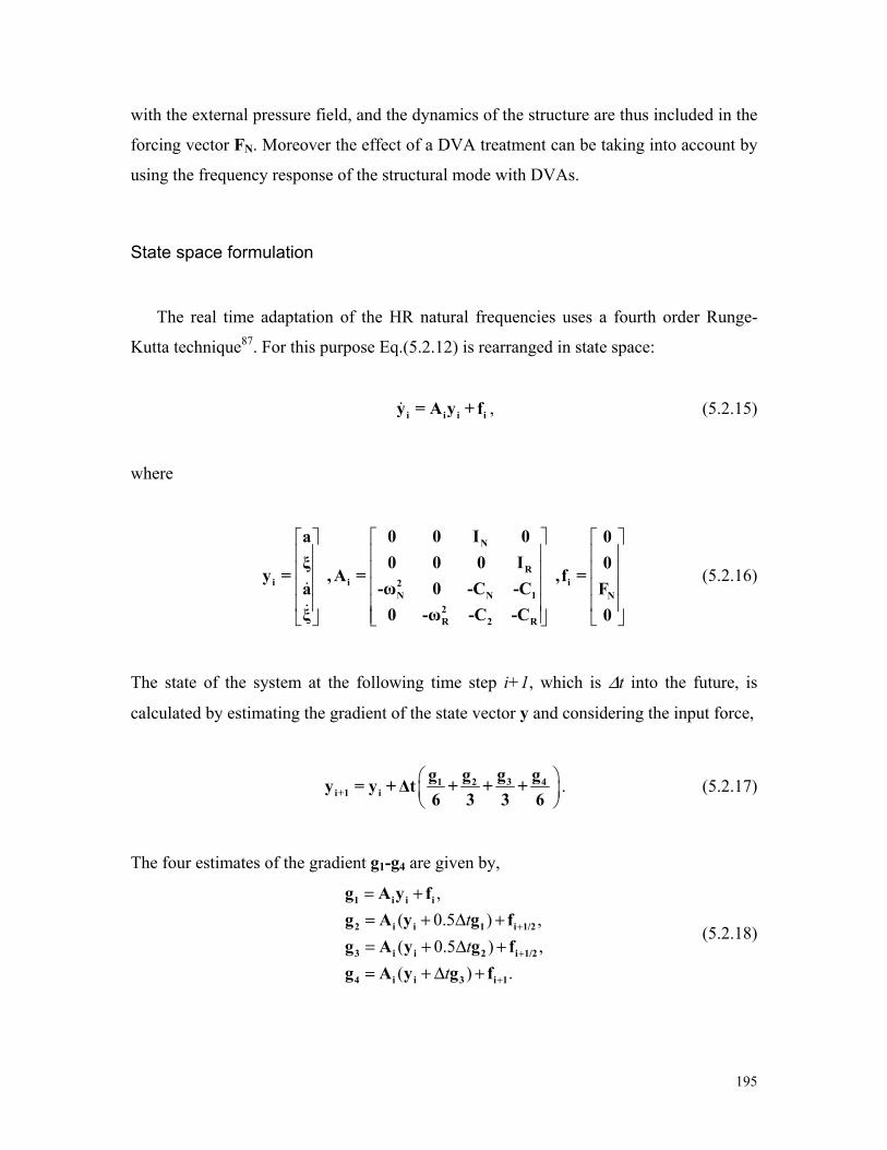
195
with the external pressure field, and the dynamics of the structure are thus included in the
forcing vector FN. Moreover the effect of a DVA treatment can be taking into account by
using the frequency response of the structural mode with DVAs.
State space formulation
The real time adaptation of the HR natural frequencies uses a fourth order Runge-
Kutta technique87. For this purpose Eq.(5.2.12) is rearranged in state space:
i i i iy = A y + f , (5.2.15)
where
N
Ri i i2
N N 1 N2R 2 R
0 0 I 0a 00 0 0 Iξ 0
y = , A = ,f =-ω 0 -C -Ca F
0 -ω -C -Cξ 0
(5.2.16)
The state of the system at the following time step i+1, which is ∆t into the future, is
calculated by estimating the gradient of the state vector y and considering the input force,
31 2 4i+1 i
gg g gy = y +∆t + + +6 3 3 6
. (5.2.17)
The four estimates of the gradient g1-g4 are given by,
,( 0.5 ) ,( 0.5 ) ,( ) .
tt
t
+
+
+
= += + ∆ += + ∆ += + ∆ +
1 i i i
2 i i 1 i 1/2
3 i i 2 i 1/2
4 i i 3 i 1
g A y fg A y g fg A y g fg A y g f
(5.2.18)
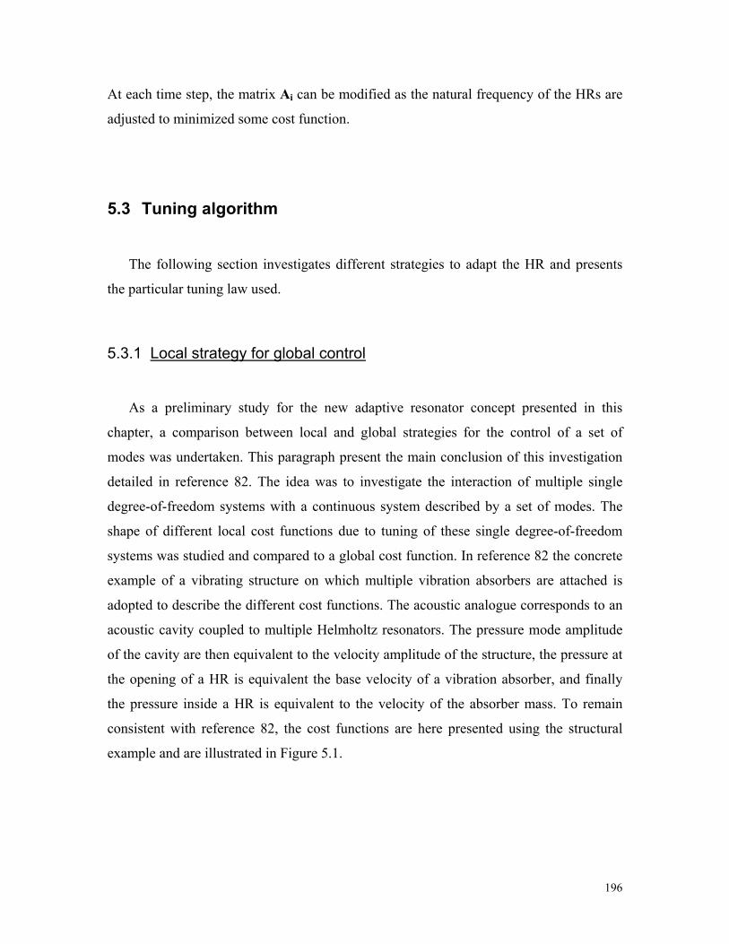
196
At each time step, the matrix Ai can be modified as the natural frequency of the HRs are
adjusted to minimized some cost function.
5.3 Tuning algorithm
The following section investigates different strategies to adapt the HR and presents
the particular tuning law used.
5.3.1 Local strategy for global control
As a preliminary study for the new adaptive resonator concept presented in this
chapter, a comparison between local and global strategies for the control of a set of
modes was undertaken. This paragraph present the main conclusion of this investigation
detailed in reference 82. The idea was to investigate the interaction of multiple single
degree-of-freedom systems with a continuous system described by a set of modes. The
shape of different local cost functions due to tuning of these single degree-of-freedom
systems was studied and compared to a global cost function. In reference 82 the concrete
example of a vibrating structure on which multiple vibration absorbers are attached is
adopted to describe the different cost functions. The acoustic analogue corresponds to an
acoustic cavity coupled to multiple Helmholtz resonators. The pressure mode amplitude
of the cavity are then equivalent to the velocity amplitude of the structure, the pressure at
the opening of a HR is equivalent the base velocity of a vibration absorber, and finally
the pressure inside a HR is equivalent to the velocity of the absorber mass. To remain
consistent with reference 82, the cost functions are here presented using the structural
example and are illustrated in Figure 5.1.
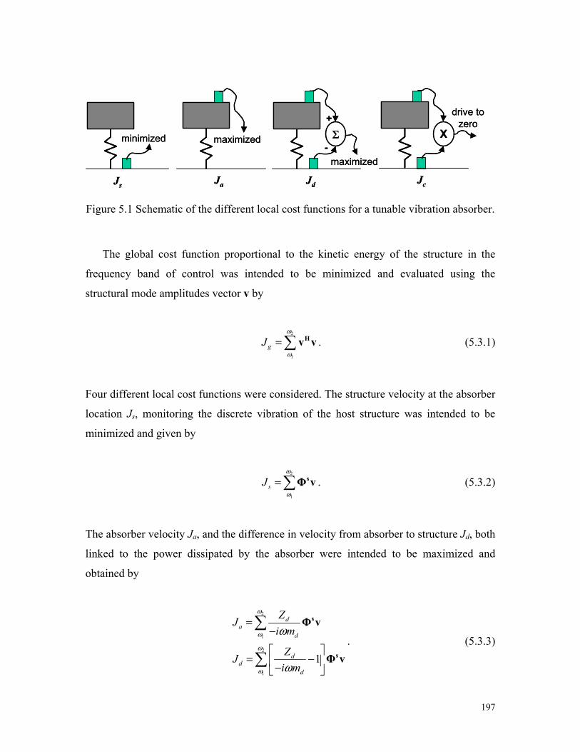
197
minimized
Js
maximized
Ja
maximized
Jd
Σ
drive to zero
Jc
X+
-minimized
Js
maximized
Ja
maximized
Jd
Σ
drive to zero
Jc
X+
-
Figure 5.1 Schematic of the different local cost functions for a tunable vibration absorber.
The global cost function proportional to the kinetic energy of the structure in the
frequency band of control was intended to be minimized and evaluated using the
structural mode amplitudes vector v by
2
1
gJω
ω=∑ Hv v . (5.3.1)
Four different local cost functions were considered. The structure velocity at the absorber
location Js, monitoring the discrete vibration of the host structure was intended to be
minimized and given by
2
1
sJω
ω=∑ sΦ v . (5.3.2)
The absorber velocity Ja, and the difference in velocity from absorber to structure Jd, both
linked to the power dissipated by the absorber were intended to be maximized and
obtained by
2
1
2
1
1
da
d
dd
d
ZJi m
ZJi m
ω
ω
ω
ω
ω
ω
=−
= − −
∑
∑
s
s
Φ v
Φ v. (5.3.3)

198
Finally the product between the velocity of the absorber and the structure, was intended
to be driven to zero and expressed as
2
1
dc
d
ZJi m
ω
ω ω
= × − ∑ s sΦ v Φ v . (5.3.4)
As shown in Figure 5.2, this latest cost function called the dot-product is the only local
cost functions of the set that converge very close to the global solution for a multi-mode
single absorber case. This remained valid for the multi-mode multi-absorber case. The
dot-product method was therefore retained as a local tuning law and its mechanisms are
analyzed in detailed in the next section.
0 20 40 60 80 100 120 140-0.4
-0.2
0
0.2
0.4
0.6
0.8
1
1.2
Tuning Frequency (Hz)
Cos
t fun
ctio
n
JgJaJdJsJc
Figure 5.2 Cost functions as a function of absorber tuning frequency using13 modes.
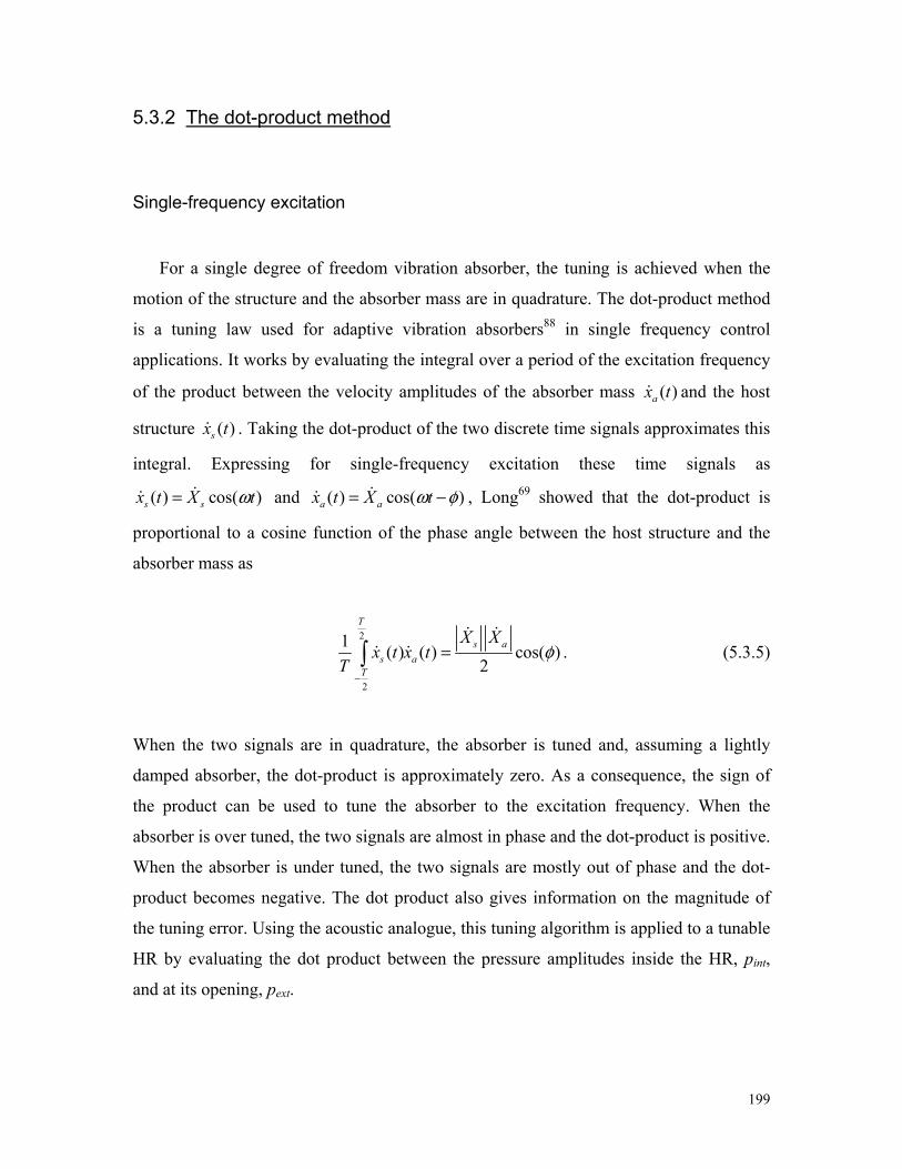
199
5.3.2 The dot-product method
Single-frequency excitation
For a single degree of freedom vibration absorber, the tuning is achieved when the
motion of the structure and the absorber mass are in quadrature. The dot-product method
is a tuning law used for adaptive vibration absorbers88 in single frequency control
applications. It works by evaluating the integral over a period of the excitation frequency
of the product between the velocity amplitudes of the absorber mass ( )ax t and the host
structure ( )sx t . Taking the dot-product of the two discrete time signals approximates this
integral. Expressing for single-frequency excitation these time signals as
( ) cos( )s sx t X tω= and ( ) cos( )a ax t X tω φ= − , Long69 showed that the dot-product is
proportional to a cosine function of the phase angle between the host structure and the
absorber mass as
2
2
1 ( ) ( ) cos( )2
T
s as a
T
X Xx t x t
Tφ
−
=∫ . (5.3.5)
When the two signals are in quadrature, the absorber is tuned and, assuming a lightly
damped absorber, the dot-product is approximately zero. As a consequence, the sign of
the product can be used to tune the absorber to the excitation frequency. When the
absorber is over tuned, the two signals are almost in phase and the dot-product is positive.
When the absorber is under tuned, the two signals are mostly out of phase and the dot-
product becomes negative. The dot product also gives information on the magnitude of
the tuning error. Using the acoustic analogue, this tuning algorithm is applied to a tunable
HR by evaluating the dot product between the pressure amplitudes inside the HR, pint,
and at its opening, pext.

200
Broadband excitation
Under broadband excitation, the product of the two signals is integrated over an
arbitrary period T. This integral provides an estimate at τ=0 of the cross correlation
function int , ( )
extp pX τ between pint and pext; the longer the period, the more accurate the
estimation. The cross correlation can be expressed as the inverse Fourier transform of the
cross spectrum G(ω) of the two signals:
int int, ,( ) ( )
ext ext
jp p p pX G e dωττ ω ω
+∞
−∞
= ∫ . (5.3.6)
Using the even and odd properties of the real and imaginary part of the cross spectrum,
the dot product reduces to
int int, ,
0
( 0) Re( ( ))ext extp p p pX G dτ ω ω
+∞
= = ∫ . (5.3.7)
As explained in section 3.2.4, for frequencies well below the first mode of the HR
cavity, Eq.(3.2.4) links the internal pressure pint and the volume velocity of the HR
opening u. Rearranging this equation yields
2
( ) ( )inth
cp ui Vρω ωω
= . (5.3.8)
The HR admittance Yh derived in section 2.5.1, relates the HR volume velocity to the
impinging pressure at its throat, pext as
2
2 2 2( ) ( ) ( ) ( )c [( ) 2 ]
h hh ext ext
h h h
i Vu Y p pi
ωωω ω ω ωρ ω ω ς ωω
= =− −
(5.3.9)
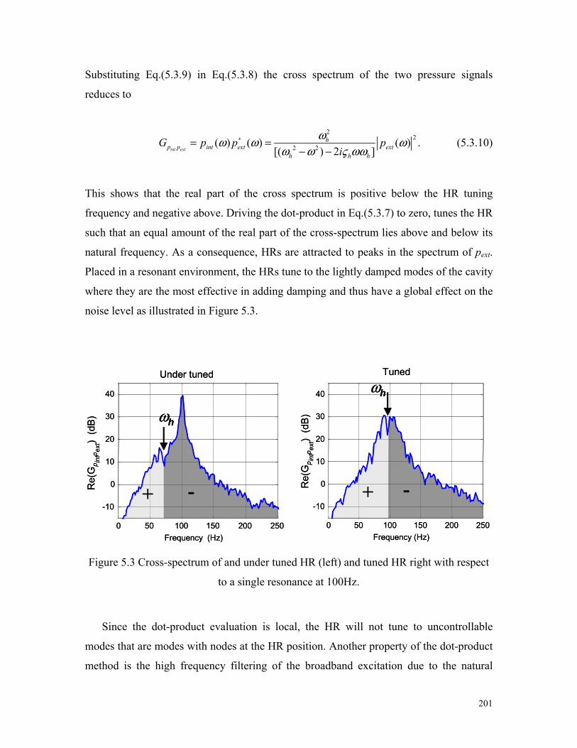
201
Substituting Eq.(5.3.9) in Eq.(5.3.8) the cross spectrum of the two pressure signals
reduces to
2
22 2( ) ( ) ( )
[( ) 2 ]int ext
hp p int ext ext
h h h
G p p pi
ωω ω ωω ω ς ωω
∗= =− −
. (5.3.10)
This shows that the real part of the cross spectrum is positive below the HR tuning
frequency and negative above. Driving the dot-product in Eq.(5.3.7) to zero, tunes the HR
such that an equal amount of the real part of the cross-spectrum lies above and below its
natural frequency. As a consequence, HRs are attracted to peaks in the spectrum of pext.
Placed in a resonant environment, the HRs tune to the lightly damped modes of the cavity
where they are the most effective in adding damping and thus have a global effect on the
noise level as illustrated in Figure 5.3.
0 50 100 150 200 250
-10
0
10
20
30
40
Frequency (Hz)
+ -
ωh
0 50 100 150 200 250
-10
0
10
20
30
40
Frequency (Hz)
+ -
ωh
Re(
Gp intp ext)
(dB)
Re(
Gp intp ext)
(dB
)
Under tuned Tuned
0 50 100 150 200 250
-10
0
10
20
30
40
Frequency (Hz)
+ -
ωh
0 50 100 150 200 250
-10
0
10
20
30
40
Frequency (Hz)
+ -
ωh
Re(
Gp intp ext)
(dB)
Re(
Gp intp ext)
(dB
)
Under tuned Tuned
Figure 5.3 Cross-spectrum of and under tuned HR (left) and tuned HR right with respect
to a single resonance at 100Hz.
Since the dot-product evaluation is local, the HR will not tune to uncontrollable
modes that are modes with nodes at the HR position. Another property of the dot-product
method is the high frequency filtering of the broadband excitation due to the natural

202
dynamics of the HR. Indeed the displacement-force admittance of the HR provides a -
6dB per decade filter above the tuning frequency. Excited with a constant volume
velocity source, the acoustic resonances of the cavity present a velocity-force admittance
behavior with symmetric slopes of 3dB and –3dB per decade before and after the natural
frequency. Combining these two type of responses with Eq.(5.3.10) leads to band-passed
filter properties for the cross-spectrum. However if the cavity is excited by a constant
volume acceleration source, the acoustic resonances present the same displacement-force
admittance behavior as the resonator. As a consequence, the cross-spectrum behave as a 6
order low-pass filter. This may cause an under tuning of the HR by biasing the dot
product to the low frequencies. Therefore, when the cavity is excited with a constant
acceleration source such as a speaker, the dot-product can be evaluated using the
derivative of the pressure signals. The resulting cross-spectrum presents band-passed
filter properties, which ensure a more accurate tuning.
In the model, the pressures inside the HR and at its throat are expressed as
2
,
( 1,... )
( 1,... )
int hh
aout h N N
N
cp i nV
p a i n
ρ ξ
ρ φ
= =
= − =∑, (5.3.11)
where n is the number of time steps defining the period T. In order to limit its absolute
value by unity, the dot product, xp, is also normalized
( )( )
int outp
int int out out
p pxp p p p
⋅=⋅ ⋅
. (5.3.12)
5.4 Numerical simulations
The following numerical simulations correspond to the Boeing composite cylinder.
The natural frequencies and mode shapes for the acoustic cavity are obtained from

203
section 2.3. The structural modal characteristics differ slightly from those presented in
section 2.2 as the simpler Donnell-Musthari shell theory72 was used. The length of the
HR neck was chosen to modify their tuning frequency.
5.4.1 Single mode forced by an internal source
In this section the acoustic forcing is provided by a piston source inside the cavity;
therefore, because the model is only one-way coupled, the dynamics of the structure do
not intervene in the computation. The source modeled as a random signal is positioned at
the bottom of the cylinder (axial position z=0, radial position r=1.23, and circumferential
position θ=π). Only the first mode of the cavity with a natural frequency of 61.7 Hz and a
damping ratio of 1% is taken into account. Three identical HRs are positioned at the
boundary (i.e. r=1.23), at the bottom of the cylinder (z=0) and are evenly distributed
around the circumference (θ=0, 2π/3, 4π/3). The total volume of the HRs represents
0.6% of the cavity volume. The optimal damping ratio is set to 5.2% according to
Eq.(3.3.3). The initial length of the necks are 12cm, 20 cm and 15cm, which provide
initial tuning frequencies of 66.7Hz, 55.1Hz and 62.0Hz respectively. This configuration
represents the over-tuned, under-tuned and tuned cases for the HRs. Using the Runge-
Kutta model with a time step of 1ms, the necks of HRs are sequentially adapted by
2.5mm increments according to the value of the dot product evaluated over a period of
0.5s. The HRs stop tuning when the absolute value of the normalized dot product drops
below 0.01. Figure 5.4 shows the evolution of the dot product and the tuning frequency
for the 3 HRs as a function of time. As expected the first HR drops its natural frequency
down to 62.1Hz, the second raises it to 59.6Hz and the third one maintains it at 62.0Hz.
The adaptation time for the three HRs is less than 25 s (during the first 5 seconds, HRs
are inactive).

204
0 10 20 30-0.5
0
0.5Dot product
HR
1
0 10 20 30-0.5
0
0.5
HR
2
0 10 20 30-0.5
0
0.5
HR
3
time (s)
0 10 20 3055
60
65
HR tuning frequency (Hz)
HR
1
0 10 20 3055
60
65
HR
20 10 20 30
55
60
65
HR
3
time (s)
Figure 5.4 Change in the dot-product and tuning frequency of the 3 HRs as a function of
time.
5.4.2 Multi-mode forced by an external plane wave
In this section the acoustic cavity is forced through the structure by an incident plane
wave (αi=70°). Figure 5.5 shows the kinetic and acoustic energy obtained with the one-
way coupled frequency domain model with and without the DVA treatment. The
simulation includes 36 structural modes and 17 acoustic modes with natural frequencies
below 200Hz. The DVA treatment, representing 2% of the cylinder mass, consists of a
ring of 13 absorbers distributed evenly around the circumference and placed halfway up
the cylinder wall. The damping ratio of the structural mode is set to 1% whereas the
damping ratio of the DVAs is set to its optimal value of 10% computed using Eq.(3.3.1).
The DVAs target the most excited 1,2 structural mode at 112.5Hz, which also couples
best to the acoustic cavity. Once this structural resonance is damped by the DVAs, the
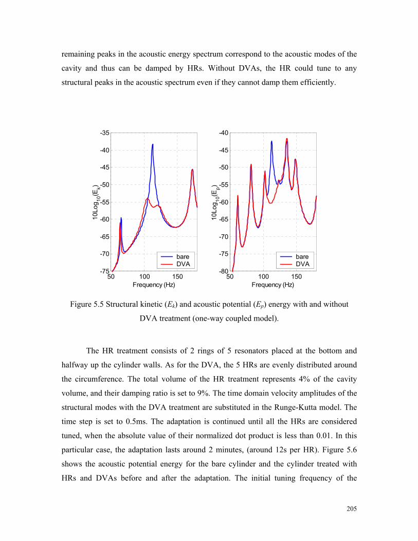
205
remaining peaks in the acoustic energy spectrum correspond to the acoustic modes of the
cavity and thus can be damped by HRs. Without DVAs, the HR could tune to any
structural peaks in the acoustic spectrum even if they cannot damp them efficiently.
50 100 150-75
-70
-65
-60
-55
-50
-45
-40
-35
10Lo
g 10(E
k)
Frequency (Hz)
bareDVA
50 100 150-80
-75
-70
-65
-60
-55
-50
-45
-40
10Lo
g 10(E
p)
Frequency (Hz)
bareDVA
Figure 5.5 Structural kinetic (Ek) and acoustic potential (Ep) energy with and without
DVA treatment (one-way coupled model).
The HR treatment consists of 2 rings of 5 resonators placed at the bottom and
halfway up the cylinder walls. As for the DVA, the 5 HRs are evenly distributed around
the circumference. The total volume of the HR treatment represents 4% of the cavity
volume, and their damping ratio is set to 9%. The time domain velocity amplitudes of the
structural modes with the DVA treatment are substituted in the Runge-Kutta model. The
time step is set to 0.5ms. The adaptation is continued until all the HRs are considered
tuned, when the absolute value of their normalized dot product is less than 0.01. In this
particular case, the adaptation lasts around 2 minutes, (around 12s per HR). Figure 5.6
shows the acoustic potential energy for the bare cylinder and the cylinder treated with
HRs and DVAs before and after the adaptation. The initial tuning frequency of the
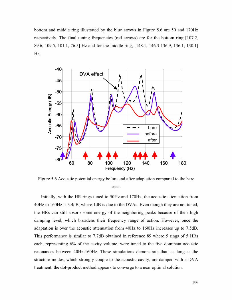
206
bottom and middle ring illustrated by the blue arrows in Figure 5.6 are 50 and 170Hz
respectively. The final tuning frequencies (red arrows) are for the bottom ring [107.2,
89.6, 109.5, 101.1, 76.5] Hz and for the middle ring, [148.1, 146.3 136.9, 136.1, 130.1]
Hz.
60 80 100 120 140 160 180-80
-75
-70
-65
-60
-55
-50
-45
-40
Frequency (Hz)
Acou
stic
Ene
rgy
(dB)
DVA effect
barebefore
after
60 80 100 120 140 160 180-80
-75
-70
-65
-60
-55
-50
-45
-40
Frequency (Hz)
Acou
stic
Ene
rgy
(dB)
DVA effect
barebefore
after
Figure 5.6 Acoustic potential energy before and after adaptation compared to the bare
case.
Initially, with the HR rings tuned to 50Hz and 170Hz, the acoustic attenuation from
40Hz to 160Hz is 3.4dB, where 1dB is due to the DVAs. Even though they are not tuned,
the HRs can still absorb some energy of the neighboring peaks because of their high
damping level, which broadens their frequency range of action. However, once the
adaptation is over the acoustic attenuation from 40Hz to 160Hz increases up to 7.5dB.
This performance is similar to 7.7dB obtained in reference 89 where 5 rings of 5 HRs
each, representing 6% of the cavity volume, were tuned to the five dominant acoustic
resonances between 40Hz-160Hz. These simulations demonstrate that, as long as the
structure modes, which strongly couple to the acoustic cavity, are damped with a DVA
treatment, the dot-product method appears to converge to a near optimal solution.

207
5.5 Experimental results
This section describes the experiment conducted on the composite cylinder. The
adaptive resonator prototype and the control system are also presented.
5.5.1 Adaptive Helmholtz resonator prototype
According to Eq.(1.4.2), changing the resonant frequency of a Helmholtz resonator
can be achieved by modifying the volume, the opening area or the neck length. De
Bedout et al. built a tunable resonator with a variable volume65. This solution probably
allows the widest tuning range and ensures the natural frequency to vary as the square
root of the volume. However, the HR efficiency is proportional to its volume (section
2.5.1), and therefore this device has reduced efficiency when tuned above its lowest
frequency. In addition, the weight of the machinery required to change a sealed volume
renders such a device unsuited for payload fairing applications.
Several designs of tunable HR with fixed volume were investigated. The best
compromise between tuning range and compactness was obtained for a variable opening
HR as shown in Figure 5.7. Based on the previous design, the resonator was made of a
cardboard tube with plastic end-caps. On the top end-cap, an iris diaphragm provides the
variable opening whose diameter ranges from 9 to 58mm. The length of the tube (22”)
was chosen to obtain a tuning range including the first three acoustic mode of the
cylinder at 63, 82, and 103Hz. Using a pulley mechanism, a lightweight (28g) small step
motor is used to rotate the iris control arm as shown in Figure 5.8. This mechanism
represented an easy, off the shelf and cheap solution. The adaptive HR is equipped with
two microphones; one placed in front of the opening, and the other flush mounted to the
back end cap to monitor the internal pressure. These two microphones provide the two
signals needed to evaluate the dot product.

208
XXXX
Figure 5.7 Adaptive Helmholtz resonator prototype.
Figure 5.8 Motorized iris diaphragm mechanism.
Using the same experimental set-up as described in Figure 3.35, the adaptive HR
natural frequency and damping ratio were measured for different opening diameters.
Because of the 90° minimum step angle of the motor, only 30 different diameters can be
obtained. The resulting frequency resolution of approximately 2Hz is sufficient for this
Step motor
Cardboard tube
22”
Iris diaphragm
Iris diaphragm
Motor shaft
Pulley
microphones
209
particular application, which requires damped HRs. As shown in Figure 5.9, the good
agreement between the measured and the predicted natural frequency using Eq.(1.4.2) is
lost for opening diameters greater than 30mm. This is due to the increase of the aperture
thickness as the iris opens. Indeed, in Eq.(1.4.2), the physical neck is fixed to 1mm,
which corresponds to the thickness of the iris for small diameter. However, as the leaves
of the iris fold to open, the physical neck increase to a maximum that includes the frame
and end-cap thickness. Using a neck length corresponding to each opening diameter in
Eq.(1.4.2) can correct this discrepancy. As illustrated in Figure 5.9, the damping of the
resonator also varies significantly with the tuning frequency. Created by viscous losses,
the damping increase non-linearly as the HR opening is reduced. A fairly constant level
of damping through out the frequency range is preferable to ensure the optimal
perfromance of the HR. As a solution, a wire mesh screen is placed over the opening to
increase the damping levels, for diameters greater than 20mm. To avoid a further increase
of damping, already too high for smaller diameters, a 20mm diameter disk is cut out of
the center of the screen as shown in Figure 5.10. The measured natural frequency and
damping ratio with and without screen is plotted in Figure 5.11 as well as the theoretical
frequency obtained with adjusted neck length. The resonance of the HR is not affected by
the presence of the screen and can be well predicted by Eq. (1.4.2). In addition, the screen
ensures a more constant and favorable damping level of 5% throughout the tuning range
except for the lowest three frequencies.

210
10 15 20 25 30 35 40 45 5050
100
150
opening diameter (mm)
Freq
uenc
y (H
z)
theory measured
10 15 20 25 30 35 40 45 500
5
10
opening diameter (mm)
Dam
ping
ratio
(%) measured
Figure 5.9 Measured natural frequency and damping ratio without screen for different
opening diameters.
Figure 5.10 Iris diaphragm with wire mesh screen for constant damping.
Iris diaphragm
Screen

211
10 15 20 25 30 35 40 45 5040
60
80
100
120
opening diameter (mm)
Freq
uenc
y (H
z)theory no screen with screen
10 15 20 25 30 35 40 45 500
5
10
opening diameter (mm)
Dam
ping
ratio
(%) no screen
with screen
Figure 5.11 Measured natural frequency and damping ratio with screen for different
opening diameters.
5.5.2 Control system
The main advantage of this method is its possible implementation using analogue
circuitry, which reduces the controller complexity, cost, and weight. Indeed, the analogue
signals of the two microphones can be summed and then low pass filtered yielding a
positive or negative continuous voltage that can then control the rotation of a standard
DC motor. To avoid tuning the HR outside of its functional range band pass filtering of
the two microphone signals around this range would be sufficient. This simple scheme
permits the integration of sensor, actuator and controller into one generic device.
However, in this work, a digital centralized controller was developed to mimic the
behavior of multiple independent analogue controllers. This centralized controller was
more suitable to observe the tuning mechanisms of several HRs simultaneously. This

212
control system uses a Labview interface and is composed of two parts. The first part is
the National Instrument data acquisition used to acquire the time signals of the
microphone. The second is the stepper motor driver, which uses the parallel port of the
computer and an electronic circuit composed of decoders and transistor arrays. A 5 volt
and 28 volt power supply is required for the electronics and the stepper motor
respectively. This system allows the control of up to eight motors sequentially. Given the
initial diameter of the opening, the system tracks the iris variations and stops the motor
whenever the physical limits of the opening are reached.
Figure 5.12 Control system for 8 resonators.
5.5.3 Experimental set-up
Eight adaptive HRs identical to the one in Figure 5.7 each equipped with two
microphones were built. A speaker was placed at the bottom of the cylinder as seen in
Figure 5.13 and driven with 40-200Hz band passed white noise to excite the acoustic
cavity. Three rings of five microphones positioned at 19, 54, 92 inches from the bottom
and 12 inches from the wall were used to obtain a spatial average of the acoustic pressure
Dual power supply
Electronic circuit
Motor cable
Parallel port

213
inside the cylinder. A last microphone was placed inside the disturbance speaker cabinet
in order to estimate the volume velocity (VV) of the source as explained in section 3.2.4.
The auto-spectra of all the microphones and their cross-spectrum with respect to the
microphone placed inside the speaker cabinet can be acquired simultaneously. The total
volume of the resonator represents only 0.4% of the cylinder’s cavity. As a consequence,
to obtain the best efficiency, the 8 HRs are positioned as illustrated in Figure 5.7 with
their opening towards the cylinder wall. In this configuration, the HRs are placed at
antinodes of the first three acoustic modes (1,0,0), (0,1,0) and (1,1,0), which orient with
respect to the disturbance speaker.
Figure 5.13 Top view of the inside of the cylinder
Speaker
Cylinder wall
Adaptive HRs
Microphones

214
5.5.4 Results
The microphone signals are first acquired when the HRs are inside the cylinder with
tape over their opening which renders them inactive. This configuration is called “bare”
since it is equivalent to the empty cylinder apart from the small volume taken by the HR.
The tape is then removed from the HR throats and the opening diameters are set to some
initial value. The data is acquired in this configuration, which is called “before
adaptation”. The control system is turned on, and using the time signal of the HR
microphones the adaptation begins. When the opening diameter of each HR has
converged, the control is turned off and all the sensor signals are acquired to evaluate this
“after adaptation” configuration.
Single mode tuning
The objective of this experiment was to verify the tuning algorithm on a single mode.
The HR microphones signals were therefore digitally band-pass filtered around the third
mode of the acoustic cavity at 103Hz. The cut-on frequencies of the 6th order Butterworth
filters used were 95 and 115Hz. As explained previously the time derivative of the
microphone signals are used to compute the dot-product. The opening diameters of the
HR were set initially to 12 mm and the 8 HRs were adapted sequentially. With a
sampling frequency of 1024Hz, the dot-product was evaluated over one second using
1024 points and its threshold below which the HRs were considered tuned was set to
0.05. The adaptation process was carried on for about 5 minutes, each iteration lasting
about one second. Figure 5.14 plots the opening diameter of the 8 HRs for every iteration.
and Table 5.1 lists the corresponding initial and final tuning frequencies obtained from
the transfer function between the two microphones at each HR. As an example, the
transfer function of two HR before and after adaptation is plotted in Figure 5.15 showing
the shift in their natural frequency. Note that these transfer functions are obtained as a
ratio of the cross spectrum of the two microphone with respect to the microphone placed
in the speaker cabinet, and the spike around 90Hz comes the ratio of a zero in both cross

215
spectra. To further illustrate the convergence of the HRs toward the 104Hz-targeted
resonance, Figure 5.16 plot for two HRs the real part of the normalized cross-spectrum
after band-passed filtering. Initially under tuned, the arithmetic area under the blue curve
corresponding to the dot-product value xp is negative. Once tuned, the positive and
negative area under the red curve balances out yielding a dot-product value close to zero.
0 50 100 150 200 250 30010
15
20
25
30
35
40
45
50
Iteration
Ope
ning
dia
met
er (m
m)
Figure 5.14 Evolution of the opening diameter for the 8 HRs.
Tuning frequency (Hz)
HR # Before adaptation After adaptation 1 72 105.5 2 69 105 3 66 104.5 4 67 105 5 69 108 6 70 101.5 7 67 101 8 67 106
Table 5.1 Tuning frequency of the 8 HR before and after the single mode adaptation.

216
60 70 80 90 100 110 1200
5
10|tr
ansf
er fu
nctio
n| (d
B)
Frequency (Hz)
HR#2
beforeafter
60 70 80 90 100 110 120-170
-130
-90
-50
-10
Frequency (Hz)
phas
e (d
egre
e)
beforeafter
60 70 80 90 100 110 1200
5
10
|tran
sfer
func
tion|
(dB
)
Frequency (Hz)
HR#8
beforeafter
60 70 80 90 100 110 120-170
-130
-90
-50
-10
Frequency (Hz)
phas
e (d
egre
e)
beforeafter
Figure 5.15 Magnitude and phase of the transfer function of HRs #2 and #8.
60 80 100 120-0.4
-0.35
-0.3
-0.25
-0.2
-0.15
-0.1
-0.05
0
0.05
0.1
Rea
l par
t of n
orm
aliz
ed c
ross
-spe
ctru
m
Frequency (Hz)
HR#4
before xp=-0.88after xp=0.05
60 80 100 120-0.4
-0.35
-0.3
-0.25
-0.2
-0.15
-0.1
-0.05
0
0.05
0.1
Rea
l par
t of n
orm
aliz
ed c
ross
-spe
ctru
m
Frequency (Hz)
HR#6
before xp=-0.86after xp=-0.04
Figure 5.16 Normalized cross-spectrum of HR#4 and HR#6.
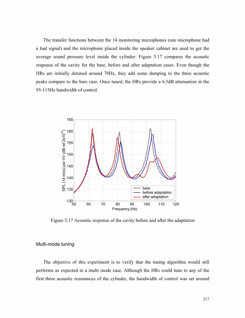
217
The transfer functions between the 14 monitoring microphones (one microphone had
a bad signal) and the microphone placed inside the speaker cabinet are used to get the
average sound pressure level inside the cylinder. Figure 5.17 compares the acoustic
response of the cavity for the bare, before and after adaptation cases. Even though the
HRs are initially detuned around 70Hz, they add some damping to the three acoustic
peaks compare to the bare case. Once tuned, the HRs provide a 6.5dB attenuation in the
95-115Hz bandwidth of control.
50 60 70 80 90 100 110 120130
135
140
145
150
155
160
165
SP
L (1
4 m
ics)
per
VV
(dB
ref 2
x10-5
)
Frequency (Hz)
bare before adaptationafter adaptation
Figure 5.17 Acoustic response of the cavity before and after the adaptation
Multi-mode tuning
The objective of this experiment is to verify that the tuning algorithm would still
performs as expected in a multi mode case. Although the HRs could tune to any of the
first three acoustic resonances of the cylinder, the bandwidth of control was set around

218
the last two. The unavoidable high damping level of the HR near 64Hz and the sharing of
the already small 0.4% volume ratio on three different modes would not lead to
significant attenuation of the 3 peaks. The digital filter cut-on frequencies for the HR
signals were set to 75 and 115Hz, and the adaptation was carried on using the same
procedure as with the single mode experiment. Figure 5.18 illustrates the evolution of the
opening diameter and Table 5.2 lists the corresponding initial and final HR tuning
frequencies. As observed in the simulation, the HRs spread their natural frequencies
across the bandwidth of control. Figure 5.19 shows the real part of the normalized cross-
spectrum for HR#2 tuned to the second mode and HR#4 tuned to the third. In both cases
the dot-product initially negative converges towards zero. The acoustic response of the
cavity plotted in Figure 5.20 demonstrates the global effect of the tuning algorithm as
both targeted peaks are reduced by 6 and 8dB compared to before the adaptation. The
resulting overall attenuation in the 75-115Hz bandwidth of control is 4.2dB.
0 50 100 150 200 250 300 35010
15
20
25
30
35
40
45
Iteration
Ope
ning
dia
met
er (m
m)
Figure 5.18 Evolution of the opening diameter for the 8 HRs.

219
Tuning frequency (Hz)
HR # Before adaptation After adaptation 1 72 102.5 2 69 81 3 66 90 4 67 102 5 69 97 6 70 88 7 67 86 8 67 103
Table 5.2 Tuning frequency of the 8 HRs before and after the multi mode adaptation.
60 80 100 120-0.25
-0.2
-0.15
-0.1
-0.05
0
0.05
Rea
l par
t of n
orm
aliz
ed c
ross
-spe
ctru
m
Frequency (Hz)
HR#2
before xp=-0.68after xp=-0.01
60 80 100 120-0.25
-0.2
-0.15
-0.1
-0.05
0
0.05R
eal p
art o
f nor
mal
ized
cro
ss-s
pect
rum
Frequency (Hz)
HR#4
before xp=-0.8after xp=0.03
Figure 5.19 Normalized cross-spectrum of HR#2 and #4

220
50 60 70 80 90 100 110 120130
135
140
145
150
155
160
165
SP
L (1
4 m
ics)
per
VV
(dB
ref 2
x10-5
)
Frequency (Hz)
bare before adaptationafter adaptation
Figure 5.20 Acoustic response before and after adaptation.
5.6 Conclusions
A time domain version of the cylinder model presented in Chapter 2 was developed.
To simplify the formulation and obtain reasonable computational time, this time domain
model was only one way coupled. The real time simulation was obtained by a fourth
order Runge-Kutta technique after rearranging the system in state-space domain.
The dot-product method commonly used to tune absorber to single frequency
excitation was applied in a new fashion to Helmholtz resonators for broadband frequency
excitation. Using only information local to each resonator, this tuning algorithm was
more practical than global strategies for payload fairing applications. Simulations
demonstrated that multiple resonators independently controlled by the dot-product, can
lead to global broadband noise attenuation in a lightly damped enclosure. The level of
attenuation obtained was close to near optimal solution. In the case of an externally

221
forced cavity, the structural modes which couple well to the internal acoustic spectrum
must be damped by DVAs to ensure a proper tuning of the HR to acoustic peaks.
A prototype of adaptive Helmholtz resonator was built and characterized. A
centralized controller mimicking the behavior of multiple independent local controllers
was developed in order to track and observe the tuning mechanisms of up to 8 HRs
simultaneously. The experiments carried on the Boeing cylinder with 8 adaptive
resonators validated the simulations and demonstrated the ability of the dot-product
method to tune resonators to near optimal solution over a frequency band including
multiple resonances.

222
Chapter 6 Conclusions and future work
6.1 Conclusions
This work has demonstrated that a lightweight and compact noise reduction treatment
can significantly increase low frequency transmission loss of a composite cylinder
representative of a payload fairing. This is possible because in such structures the lower
part of the internal acoustic spectrum is composed of sharp structural and acoustic
resonances, which cannot be effectively damped by traditional acoustic blankets.
Therefore, damped vibration absorbers and Helmholtz resonators represent an efficient
way to add damping to these resonances without adding a significant amount of weight or
volume.
An analytical model of a composite cylinder excited by an oblique plane wave was
developed as a first approximation to the problem. The vibration absorbers and
Helmholtz resonators were implemented in the analytical model using an impedance
matching method. The effect of theses devices on the vibration and acoustic response
were investigated using a fully coupled system. Several characteristics of such a
treatment were illustrated.
First, the noise reductions are linked to the DVA-cylinder mass ratio and to the HR-
cavity volume ratio. Trade-offs between performance and added mass and volume were
dictated by the strict weight and volume constraints associated with payload fairing
applications.
Second, the performance of the treatment is directly related to the amount of damping
initially present in the structure and in the acoustic cavity. The higher the damping ratios
of the system, the less reduction the treatment can provide. As a consequence HRs and
DVAs represent a complimentary treatment to the existing acoustic blankets, as they are
designed to work at low frequencies where these blankets are ineffective.

223
Third, as the noise reduction devices are targeting structural and acoustic modes, their
spatial locations are of importance. Because of the axisymmetry of cylinders, the devices
are split in a certain number of units that are distributed evenly around the circumference
to avoid unfavorable modal interactions. The general rule of thumb is to position
absorbers axially at antinodes of the targeted modes. However, due to the interaction and
the modal scattering of the devices, alternative optimal positions can be found.
Finally, the presence of damping in the vibration absorbers as well as in the
Helmholtz resonators is a determining factor for broadband frequency performance.
Formulas for the optimal damping ratio of both types of devices can be found in the
literature but are restricted to the control of a single mode. Nevertheless, these formulas
provide a good estimate for the optimal damping in multi-modal cases.
Finding the best treatment, given mass and volume constraints, requires a
simultaneous optimization of the tuning frequencies, locations, and damping levels of the
devices, and therefore a genetic algorithm was used. The algorithm was set to maximize
the acoustic attenuation over a specified frequency band. Due to the complexity of the
cost function, different genetically optimized treatments led to similar attenuation levels.
The genetic solutions represented a 2.4dB improvement over an iterative optimization
based on design experience. The performance robustness to changes in excitation
characteristics, the system natural frequencies, tuning frequency, damping ratio and axial
location of the devices was also investigated. In all the different cases, the performance
was shown to be fairly robust to any particular changes. However, it was demonstrated
that random treatments, where the axial positions, frequency and damping of the HRs and
DVAs were set arbitrarily, did not perform as well on average. Therefore, some
knowledge of the system, primarily natural frequency and mode shapes, permit treatment
to be found that lie in relatively shallow bowls of the cost function surface with improved
performance and good robustness. This robustness of the treatment mainly comes from
the noise reduction mechanism that is based on adding damping to lightly damped
resonances of the system.
As the interior acoustic spectrum is dominated by acoustic resonances, the Helmholtz
resonators provide more acoustic reduction than the DVAs. However, vibration absorbers
enhance the performance by damping the remaining structural resonances present in the

224
acoustic spectrum. Thus, the performance of the DVAs is closely linked to the level of
structural-acoustic coupling of the system.
The conclusions drawn from the analytical model as well as the experimental results
obtained on the Boeing cylinder prototype were used to design a HR/DVA treatment for a
full size fairing. The analytical model was modified to use mode shapes and natural
frequencies derived using a finite element model of a fairing, and the numerical
equivalent source technique was applied in order to model the external acoustic
excitation. Although the treatment design procedure was similarly based on both iterative
and genetic optimizations, more implementation constraints such as size and location of
the devices were taken into consideration. In this regard, an effort was made to minimize
the weight of the HR treatment. Indeed, using light PETG tubes, the 212 HRs only
represent 5% of the bare fairing weight when the former foam treatment represents 10%.
The new fairing treatment composed of HRs embedded in the new, lighter foam blanket
is only 5% heavier than the former blanket and 25% by addition of the DVAs. This final
design was tested in a payload fairing and lead to 3.2dB attenuation from 30Hz to 90Hz
in agreement with the model predictions.
The other part of this work was the investigation of a new type of adaptive Helmholtz
resonator. It was shown that the dot product method usually used to track single
frequency disturbances could be useful in tracking modes driven by broadband excitation.
This could be of particular interest as the acoustic natural frequencies of a fairing’s cavity
are shifted with varying payload fills. In addition, this tuning law only requires
information local to the resonator, greatly simplifying its implementation. A time domain
model of adaptive Helmholtz resonators coupled to a cylinder was developed. The
simulations demonstrated that multiple adaptive HRs could lead to broadband noise
reductions similar to the ones obtained by genetic optimization. Experiments using
adaptive HR prototypes confirmed their ability to converge to a near optimal solution in a
frequency band including multiple modes.

225
6.2 Future work
As a first improvement of the acoustic treatments using HRs and DVAs, the
sensitivity to arbitrary payload fills could be investigated. Although the robustness of a
treatment with respect to changes in the cavity mode shapes was not strictly investigated
in this work, it can be related to the treatment robustness with respect to the axial
positions of the devices. Indeed, the treatment performance was showed to be most
sensitive to this particular parameter. Therefore, to evaluate the robustness of a treatment
designed with an empty fairing model to changes in the mode shapes and resonant
frequencies due to a payload, a finite element model could be used to model the cavity
with a variety of fills representative of typical payloads and the modes incorporated into
the analytical model developed in this work. Depending on the loss in performance, it
could be determined whether or not the treatments need to be tailored for fairings filled
with a particular payload.
For further improvement of treatments, a better knowledge of the external disturbance
acoustic field would be of interest. In this work, the devices are used in rings designed to
be independent of the azimuth angle of excitation, which is assumed to be unknown. An
accurate description of the acoustic disturbance, characteristic of a particular launch site
and launch vehicle, could lead to a better use of the noise reduction devices. Developing
an analytical model of this type of external disturbance is relatively complex and
therefore the measured acoustic field based on scaled model tests has been used
previously2. The measured disturbance can then be approximated in an analytical model
with multiple plane waves.
To increase the transmission loss of existing composite payload fairing, the use of
active/passive hybrid treatment could also be investigated. The goal would be to increase
the performance of the passive devices by using structural and acoustic actuators under a
feedforward/feedback active control scheme. The location of the reference and error
sensors is of primary importance for the effectiveness of such a treatment. To implement
this system into a real application, the development of lightweight powerful actuators is
necessary and has already been subject to investigations.

226
Another means by which to assess the problem would involve a new design of the
fairing structure itself, taking into account the acoustic transmission loss while meeting
the structural requirements. This concept is being evaluated through the use of a Chamber
Core90, where the structure is fabricated from multi-layered composite face sheets
separated by channel-shaped chambers. In addition to providing a strong and lightweight
fairing, the chambers could act as acoustic resonators able to attenuate low frequency
acoustic resonances. Another way would be to replace the honeycomb core present in
actual composite fairings with a more irregular grid. The shape and characteristics of this
grid would modify the fairing stiffness locally and could be optimized to improve the
transmission loss at low frequencies.
Furthermore, the use of thick (couple of feet) acoustic blankets placed at the bottom
and in the nose of the fairing, could damp the first axial acoustic modes and hence
increase the acoustic absorption in the low frequencies.
Finally, the concept of an adaptive Helmholtz resonator under local control for
broadband noise reduction could be extended to adaptive vibration absorbers to control
broadband vibrations of the structure. The investigation of different control architectures
(namely, hierarchical or decentralized architectures) has already commenced91. The
impact on the acoustic radiation and transmission would be of a special interest for
payload fairing applications.

227
Appendix A Acoustic damping scaling
The objective of this experiment is to determine the amount of 2-inch thick foam
needed in the cylinder prototype in order to match the reverberation time measured in the
real payload fairing.
Reverberation time of a payload fairing
The reverberation time in the payload fairing was evaluated by measuring the
response to the shut off of an acoustic source at 32 microphones. The data provided by
Boeing initially sampled at 48000 Hz was down-sampled to 3000 Hz using Matlab.
Figure A.1 shows the spatial mean squared using 31 microphone signals (one microphone
being noisy).
0 0.2 0.4 0.6 0.8 1 1.20
0.5
1
1.5
2
2.5
3
3.5x 10
-3
time (s)
mea
n sq
uare
d pr
essu
re (
31 m
ic.)
Figure A.1 Mean square pressure response to the source shut-off for the payload fairing.
The microphone signals are then digitally filtered in each 1/3rd octave band. The 31
filtered signals are squared and summed. The resulting signal proportional to the acoustic

228
potential energy is then convolved with a rectangular window. The slope of the linear
portion of this decaying signal approximates the reverberation time (T60), which is
defined as the time necessary for the sound to decay by 60 dB. Figure A.2 shows an
example of the decaying signal.
0 0.2 0.4 0.6 0.8 1 1.2-30
-25
-20
-15
-10
-5
0
5
10
time (s)
filte
red
mea
n sq
uare
d pr
essu
re (3
1 m
ic.)
dB
100 Hz 1/3 octave band
Figure A.2 100 Hz third octave band decaying signal for the payload fairing.
Reverberation time in the cylinder prototype:
The reverberation time in the cylinder prototype was evaluated by measuring the
response of 16 microphones randomly spaced in the cavity to the shut off of an acoustic
source. A speaker placed inside the cylinder with an input band passed from 31.5 to
300Hz white noise signal provided the source. The sampling frequency was 3000 Hz,
Figure A.3 shows the spatial mean squared signal.

229
1.5 1.7 1.9 2.1 2.3 2.50
0.2
0.4
0.6
0.8
1
1.2
1.4
1.6
time (s)
mea
n sq
uare
d pr
essu
re (1
6 m
ic.)
Figure A.3 Mean square pressure response to the source shut-off for the bare cylinder.
The same processing as for the payload fairing data was applied to extract the third
octave band reverberation time. Because the volume of the cylinder prototype is 16 times
smaller than the payload fairing, the lowest significant 1/3rd octave band for the cylinder
is the 40 Hz band. To determine the amount of foam necessary for matching the fairing
reverberation time, a iterative percentage of the cylinder’s wall were covered with 2-inch
thick acoustic foam panels and the T60 was evaluated in each case. Table A.1 lists the
T60 for the fairing, the bare cylinder, and the cylinder covered with 20% 40% a 100% of
foam. From these results, an approximate half coverage of the cylinder wall was chosen
to be the most representative of the damping provided by the acoustic blankets in the
fairing.

230
Reverberation time (second) Third octave band center
frequency (Hz) Payload fairing
Bare Cylinder
20% foam Cylinder
40%foam Cylinder
100%foam Cylinder
25 3.1 - - - - 31.5 2.3 - -- - - 40 2.7 3.5 3.2 2.7 1.2 50 2.7 3.6 2.7 2.2 1 63 1.8 3.5 3.1 2.1 0.9 80 1.0 1.8 1.1 1.1 1.4
100 1.3 2.1 1.6 1.2 1.4 125 0.6 1.8 1.8 1.1 2.0 160 0.4 1.6 1.6 0.8 2.1 200 0.3 4.2 1.5 0.3 1.5
Table A.1 Comparison of the third octave band reverberation time.

231
Bibliography 1 K. M. Eldred, “Acoustic loads generated by the propulsion system,” NASA SP-8072
1971. 2 J. Varnier, J. F. Piet, D. Gély, G. Elias and S. Radulovic, “Modeling of the acoustic
environment on the Ariane 5 fairing using small scale test data” proceeding of the 2nd
AIAA/CEAS, Aeroacoustics Conference, paper 96-1721, State College PA, (1996). 3 B. Troclet, B. Chemoul, P. Roux, D. Gély and G. Elias, “Synthesis of vibroacoustic
studies performed during Ariane 5 program” 1er Colloque Européen sur la Technologie
des Lanceurs “Vibration des Lanceurs” Toulouse, France, (1999). 4 S. Alestra, I. Terrasse and B. Troclet, “Identification of acoustic sources at launch
vehicle lift-off using an inverse method” proceeding of the 40th AIAA Aerospace
Sciences Meeting& Exhibit, 2002-0926, Reno, NV, (2002). 5 C. Niezrecki and H. H. Cudney, “Preliminary review of active control technology
applied to the fairing acoustic problem” AIAA/ASME/AHS Adaptive Structures Forum,
paper 96-1275, pp 101-108, Reston, VA, (1996). 6 D. J. Leo and E. H Anderson, “Vibroacoustic modeling of a launch vehicle payload
fairing for active acoustic control” proceeding of the 99th Structures, Structural
Dynamics, and Materials conference, 3212-3222 (1998). 7 S. Griffin, C. Hansen and B. Cazzolato, “Feasibility of feedback control of transmitted
sound into a launch vehicle fairing using structural sensing and proof mass actuator”
AIAA journal, paper 99-152, pp 2592-2602, (1999). 8 J. P. B. Clarke and C. Gutiérrez, “unidirectional active acoustic control for launch
vehicle fairings”, AIAA 38th Aerospace Sciences Meeting & Exhibit, paper 2000-0612,
Reno, NV, (2000). 9 J. K. Wong and J. P. B. Clarke, “Implementation of a multi-layer active structural-
acoustic transmission control” 7th AIAA/CEAS Aeroacoustics Conference, paper 2001-
2275, Maastricht, Netherlands, (2001).

232
10 S. R. Vadali and A. Das, “Active control of structural-acoustic systems- Noise
reduction in payload fairings” AIAA, Guidance, Navigation and Control Conference,
paper 96-3756, San Diego, CA, (1996). 11 M. E. Johnson and S. J. Elliott, “Experiments on the active control of sound
transmission into a stiff cylinder using a piezoelectric actuator,” Proceedings Inst.
Acoust. 16(1), 201-210 (1994). 12 C. Niezrecki, “Structural & internal acoustic response of cylinders with applications to
rocket payload fairings” Ph.D. Thesis Virginia Polytechnic Institute & State University,
1999. 13 S. A. Lane, J. D. Kemp, S. Griffin and R. L. Clark, “Active acoustic control of a rocket
fairing using spatially weighted transducer arrays”, Journal of Spacecraft and Rockets
38(1), 112-119, (2001). 14 B. H. Houston, M. H. Marcus and J. A. Bucaro, “Active blankets for the control of
payload fairing interior acoustics” AIAA Journal, (1997). 15 O. Lacour, M. A. Galland and D. Thenail, “Preliminary experiments on noise reduction
in cavities using active impedance changes”, Journal of Sound and Vibration 230(1), 69-
99 (1999). 16 C. A. Merchant and J. P. B. Clarke, “Active acoustic reflection control using glow
discharge plasma panels” 7th AIAA/CEAS Aeroacoustics Conference, paper 2001-2218,
Maastricht, Netherlands, (2001). 17 B. K. Henderson, S. A. Lane, J. Gussy, S. Griffin and K. M. Farinholt, “Development
of an acoustic actuator for launch vehicle noise reduction” Journal of the Acoustical
Society of America, 111(1), 174-179, (2002). 18 A. F. Harris, “Multi degree-of-freedom passive and active vibration absorbers for the
control of structural vibration” Masters Thesis, Virginia Tech, (2003). 19 M. E. Johnson and O. Sacarcelik, “Reference signal requirements for the feedforward
control of sound transmission into a payload fairing”, Proceedings of Noise-Con 2003,
Cleveland, OH, (2003).

233
20 W. O. Hughes, A. M. McNelis and H. Himelblau, “Investigation of acoustic fields for
the Cassini spacecraft: reverberant versus launch environments” AIAA journal paper 99-
1985, pp 1193-1203, (1999). 21 V. Martin and A. Bodrero, “An introduction to the control of sound fields by
optimizing impedance locations on the wall of an acoustic cavity”, Journal of Sound and
Vibration 204(2), 331-3357 (1997). 22 D. Gély, G. Elias, N. Lupoglazoff, F. Vuillot and F. Micheli, “Aeroacoustic
characterization and numerical simulation of Helmholtz resonator”, AIAA journal paper
99-1941, (1999). 23 I. U. Borchers, S. T. Laemmlein, P. Bartels, A. Rausch, M. Faust, J. A. F. Coebergh,
and K. Koeble, “Acoustic protection on payload fairings of expendable launch vehicles”
US Patent Number 5,670,758 (1997). 24D. C. G. Eaton and F. Betti, “Further assessments of the effects of helium and test
chambers on payload response,” Proceedings of the International Conference on
Spacecraft Structures, Materials & Mechanical Testing, Noordwijk, Netherlands, 243-257
(1996). 25 P. Gardonio, N. S. Fergusson and F. J. Fahy, “A modal expansion analysis of the noise
transmission through circular cylindrical shell structure with blocking masses,” Journal of
Sound and Vibration 244(2), 259-297 (2001). 26 H. Frahm, “Device for Damping Vibrating Bodies,” German Patent Serial Number
525,455, 1909, U.S. Patent Serial Number 989,958, (1911). 27 A. H. von Flotow, A. Beard and D. Bayley, “Adaptive tuned vibration absorbers:
tuning laws, tracking agility, sizing, and physical implementations” Noise-Con 94, pp
437-452, FL, (1994). 28 J. P. den Hartog, “Mechanical Vibrations”, (Dover Publication Inc., New York, 1985),
Chap.3, pp 93-106 (1934). 29 B. G. Korenev and L. M. Reznikov, Dynamic Vibration Absorbers, (Wiley, New York,
1993), Chap.1, p 62.

234
30 E. Pennestrì, “An application of Chebyshev’s min-max criterion to the optimal design
of a dynamic vibration absorber”, Journal of Sound and Vibration 217(4), 757-765
(1998). 31 H. J. Rice, “Design of multiple vibration absorber systems using modal data” Journal
of Sound and Vibration 160(2), 378-385 (1993). 32 D. A. Rade and V. Steffen, “Optimization of dynamic vibration absorbers over a
frequency band”, Mechanical Systems and Signal Processing 14(5), 679-690 (2000). 33 J. M. Verdirame and S. A. Nayfeh, “Design of multi-degree-of-freedom tuned mass
dampers based on eigenvalue perturbation”, Proceedings of the 11th AIAA/ASME/AHS
Adaptive Structures Conference Norfolk, Virginia (2003). 34 T. Iguza and K. Xu, “Vibration control using multiple tuned mass dampers”, Journal of
Sound and Vibration 175(4), 491-503 (1994). 35 A. S. Joshi and R. S. Jangid, “Optimum parameters of multiple tuned mass dampers for
base-excited damped systems” Journal of Sound and Vibration 202(5), 657-667 (1997). 36 M. R. Jolly and J. Q. Sun, “Passive tuned vibration absorbers for sound radiation
reduction from vibrating panels,” Journal of Sound and Vibration 191(4), 577-583
(1996). 37 Z. Sun, J. Sun, C. Wang and Y. Dai, “Dynamic vibration absorbers used for increasing
the noise transmission loss of aircraft panels” Applied Acoustics 48(4), 311-321 (1996). 38 K. Nagaya and L. Li, “Control of sound noise radiated from a plate using dynamic
absorbers under the optimization by neural network,” Journal of Sound and Vibration
208(2), 289-298 (1997). 39 G. W. Stubbs, “Tuned vibration absorbers-Practical design considerations and
application to aircraft mechanical equipment”, Proceedings of NOISE CON 96, Seattle,
WA, 497-502, (1996). 40 Y. M. Huang and C. R. Fuller, “The effects of dynamic absorbers on the forced
vibration of a cylindrical shell and its coupled interior sound field,” Journal of Sound and
Vibration 200(4), 401-418 (1997). 41 Y. M. Huang and C. R. Fuller, “Vibration and noise control of the fuselage via
dynamic absorbers,” J. Vib. Acoust. 120, 496-502 (1998).

235
42 Y. M. Huang and C. C Chen, “Optimal design of dynamic absorbers on vibration and
noise control of the fuselage” Computer and Structures 76, 691-702, (2000). 43 C. R. Fuller, J. P. Maillard, M. Mercadal and A. H. von Flotow, “Control of aircraft
interior noise using globally detuned vibration absorbers” Journal of Sound and Vibration
203(5), 745-761 (1997). 44 P. E. Cambou, “A Distributed Active Vibration Absorber (DAVA) for Active-Passive
Vibration and Sound Radiation Control,” Masters Thesis, Virginia Tech, (1998). 45 P. Marcotte, C. R. Fuller and P. Cambou, “Control of noise radiated by a plate using a
distributed active vibration absorber (DAVA)” Proceedings of Active 99, Vol 1, 447-456
(1999). 46 Lord Rayleigh (J. W. S. Strutt) , The theory of sound, (New York: Dover Publications,
second edition, 1945 re-issue) Vol II p. 170, (1877). 47 U. Ingard, “On the theory and design of acoustical resonators.” Journal of the
Acoustical Society of America, 25, 1037-1061, (1953). 48 R. F. Lambert, “A study of the factors influencing the damping of an acoustical cavity
resonator” Journal of the Acoustical Society of America, 25, 1068-1083, (1953). 49 M. Alster, “improved calculation of resonant frequencies of Helmholtz resonators”
Journal of Sound and Vibration 24(1), 63-85 (1972). 50 R. C. Chanaud, “Effect of geometry on the resonance frequency of Helmholtz
resonators.” Journal of Sound and Vibration 178(3), 337-348 (1994). 51 R. C. Chanaud, “Effect of geometry on the resonance frequency of Helmholtz
resonators, part II” Journal of Sound and Vibration 204(5), 829-834 (1997). 52 A. Selamet, N. S. Dickey and J. M. Novak, “Theoretical, computational and
experimental investigation of Helmholtz resonators with fixed volume: lumped versus
distributed analysis.” Journal of Sound and Vibration 187(2), 358-367 (1996). 53 N. S. Dickey and A. Selamet, “Helmholtz resonators: one dimensional limit for small
cavity length-to-diameter ratios.” Journal of Sound and Vibration 195(3), 512-517
(1995). 54 A. Selamet, and Z. L. Ji, “Circular asymmetric Helmholtz resonators” Journal of the
Acoustical Society of America, 107(5), 2360-2369, (2000).

236
55 A. Doria, “A simple method for the analysis of deep cavity and long neck acoustic
resonators.” Journal of Sound and Vibration 232(4), 823-833 (2000). 56 F. J. Fahy and C. Schofield, “note on the interaction between a Helmholtz Resonator
and an acoustic mode of an enclosure”, Journal of Sound and Vibration 72(3), 365-378
(1980). 57 A. Cummings, “The effect of a resonator array on the sound field in a cavity”, Journal
of Sound and Vibration 154(1), 25-44 (1992). 58 A Doria, “Control of acoustic vibrations of an enclosure by means of multiple
resonators,” Journal of Sound and Vibration 181, 673-685 (1995). 59 J. S. Hsu and K. K. Ahuja, “Cavity noise control using Helmholtz resonators”, AIAA
paper 96-1675, (1996). 60 F. Urzynicok and H. H. Fernholz, “Flow induced acoustic resonator for separation
control”, Proceedings of the 1st flow control conference, AIAA paper 2002-2819, St
Louis, MS, (2002). 61 P. K. Tang and W. A. Sirignano “Theory of generalized Helmholtz resonator” Journal
of Sound and Vibration 26, 247-262 (1973). 62 R. A. Prydz, L. S. Wirt, H. L. Kuntz and L. D. Pope, “Transmission loss a multiplayer
panel with internal tuned Helmholtz resonators.” Journal of the Acoustical Society of
America, 87(4), 1597-1602, (1990). 63 R. J. Bernhard, “The state of the art of active-passive noise control”, Proceedings of
Noise-Con 94, Ft. Lauderdale, FL, (1994). 64 J. S. Lamancusa, “An actively tuned, passive muffler system for engine silencing”,
Proceedings of Noise-Con 87, The Pennsylvania State University, PA,(1987). 65 J. M. de Bedout, M. A. Franchek, R. J. Bernhard and L. Mongeau, “Adaptive-passive
noise control with self-tuning Helmholtz resonators.” Journal of Sound and Vibration
202(1), 109-123 (1995). 66 T. M. Kostek and M. A. Franchek, “Hybrid noise control in ducts”, Journal of Sound
and Vibration 237(1), 81-100 (2000).
237
67 K. Nagaya, Y. Hano and A. Suda, “Silencer consisting of a two stage Helmholtz
resonator with auto tuning control.” Journal of the Acoustical Society of America,
110(1), 289-295, (2001). 68 J. Dayou, M. J. Brennan, “Global control of structural vibration using multiple-tuned
tunable vibration neutralizers”, Journal of Sound and Vibration 258(2), 345-357 (2002). 69 T. Long, M. J. Brennan, and S. J Elliot, “Design of smart machinery installations to
reduce transmitted vibrations by adaptive modifications of internal forces,” Proceedings
of the Institution of Mechanical Engineers, Vol. 212, Part I, 215-228,(1998). 70 M. E. Johnson, C. R. Fuller, and P. Marcotte, “Optimization of distributed vibration
absorber for sound transmission into a composite cylinder,” Proceeding of the 7th
AIAA/CEAS Aeroacoustics Conference (2001). 71 E. H. Baker and G. Herrmann “Vibration of orthotropic cylindrical sandwich shells
under initial stress”. American Institute of aeronautics and Astronautics Journal 4,1063-
1070 (1966). 72 A. W. Leissa, Vibration of shells, NASA-SP-288, (1973), Chap.2, pp 31-49. 73 N. W. McLachlan, Bessel functions for engineers second edition Oxford, Clarendon
Press 1961. 74 M. Morse and K. U. Ingard, Theoretical Acoustics, (First Princeton University Press
Edition, 1986) (1968). 75 P. A. Nelson and S. J. Elliott, Active Control of Sound, (Academic Press, 1992),
Chap.10, pp 319-322. 76 G. H. Koopmann, L. Song, and J. B Fahnline, “A method for computing acoustic fields
based on the principle of wave superposition”, Journal of the Acoustical Society of
America, 86(6) 2433-2438 (1989). 77 M. E. Johnson, S. J. Elliott, K-H. Baek, and J. Garcia-Bonitto, “An equivalent source
technique for calculating the sound field inside an enclosure containing scatterring
object”, Journal of the Acoustical Society of America, 104(3) (1998). 78 F. Fahy, Sound and Structural Vibration, Academic Press (1985). 79 Junger and Feit, Sound, Structures and Their Interaction, (2nd Edition) MIT press,
Cambridge MA (1986).
238
80 D.K. Anthony and S. J. Elliott, “A Comparison of Three Methods of Measuring the
Volume Velocity of an Acoustic Source,” Journal of Audio Engineering, Vol. 39 No. 5,
355-365 (1991). 81 H. Osman, M.E. Johnson, C.R. Fuller and P. Marcotte, “Interior Noise Reduction of
Composite Cylinders Using Distributed Vibration Absorbers,” 7th AIAA/CEAS
Aeroacoustics Conference (2001). 82 M. E. Johnson and S. J. Estève, “Comparison of local and global adaptive strategies for
the control of broadband noise in an enclosure using adaptive Helmholtz resonators”
Proceedings of the Active 2002 Conference, Institute of Sound and Vibration Research,
University of Southampton, UK, (2002). 83 D. E. Goldberg, Genetic Algorithms in Search, Optimization and Machine Learning,
(Addison-Wesley Publishing Company , Inc., Reading, MA, 1989). 84 C. R. Houck, J. A. Joines and M. G. Kay A genetic Algorithm for a function
optimization: a Matlab implementation www.ie.ncsu.edu/mirage. 85 D. M. Photiadis, “The effect of wall elasticity on the properties of a Helmholtz
resonator”, Journal of the Acoustical Society of America, 90(2) (1991). 86 A. N. Norris, and G. Wickham, “Elastic Helmholtz resonators”, Journal of the
Acoustical Society of America, 93(2) (1993). 87 W. H. Press et al., “Numerical Recipes in C: The art of Scientific Computing,”
Cambridge University Press, Second edition (1992). 88 M. R. F. Kidner, and M. J. Brennan, “Varying the stiffness of a beam-like neutralizer
under fuzzy logic control”, Journal of Vibration and Acoustics Vol. 124, 90-99, (2002). 89 S. J. Estève, and M. E. Johnson, “Reduction of sound transmitted into a composite
cylinder using Distributed Vibration Absorbers and Helmholtz Resonators,” Journal of
the Acoustical Society of America, 112(6), 2040-2048, (2002). 90 E. Herup, S. Huybrechts, S. Griffin, and S. Tsai, “Method of Making Composite
Chamber Core Sandwich-Type Structures with Inherent Acoustic Attenuation,” U. S.
Patent No. 6,231,710, 2001. 91 M. Kidner, B. Baton, and M. Johnson, “Distributed sensors for active structural
acoustic control using large hierarchical control systems” to be published in the

239
Proceedings of International Mechanical Engineering Congress & Exposition
Washington, DC, November 2003.

Vita
Simon Estève was born on April 23, 1978 in Melle, France. After graduating from
Lycée Georges Brassens, Evry in 1996, he joined the Université de Technologie de
Compiègne (UTC). He received a Diplôme d’Études Universitaires de Technologie in
July 1998 after two years of general engineering studies. He then spent his first year of
mechanical engineering as an exchange student at the University of Pennsylvania in
Philadelphia. Extending his experience in the U.S., Simon completed his technician
internship at the Center for Intelligent Materials, Systems, and Structures at the Virgina
Polytechnic Institute and State University (Virginia Tech). Under the guidance of Dr.
Don Leo, he worked for 6 months on the development of highly efficient hydraulic
actuators for aircraft hydraulic system using high frequency piezoceramic pump
actuation. After a semester of engineering studies focused on acoustics, vibrations and
signal processing back at the UTC, Simon left for the U.S. in August 2000 to join the
Vibration and Acoustics Laboratories (VAL) at Virginia Tech. There, he completed his
bachelor of science degree and started under the supervision of Dr. Marty Johnson a
Ph.D. in Mechanical Engineering on payload fairing noise control funded by Boeing. In
March 2002, he received his Mechanical Engineering Diploma from the Université de
Technologie de Compiègne. After completion of his Ph.D. in May 2004, he remained at
VAL as a research associate to work on efficient binaural simulations of structural
acoustic data for AuSIM,Inc., company specialized in virtual acoustic technologies.