Construction of Risk-Averse Enhanced Index Funds

Miguel Lejeune ∗ Gulay Samatlı-Pac†

Abstract: We propose a partial replication strategy to construct risk-averse enhanced index funds. Our model

takes into account the parameter estimation risk by defining the asset returns and the return covariance terms as

random variables. The variance of the index fund return is forced to be below a low-risk threshold with a large

probability, thereby limiting the market risk exposure of the investors and the moral hazard associated with the

wage structure of fund managers. The resulting stochastic integer problem is reformulated through the derivation

of a deterministic equivalent for the risk constraint and the use of a block decomposition technique. We develop

an exact outer approximation method based on the relaxation of some binary restrictions and the reformulation of

the cardinality constraint. The method provides a hierarchical organization of the computations with expanding

sets of integer-restricted variables and outperforms the Bonmin and the Cplex 12.1 solvers. The method

can solve very large (up to 1000 securities) instances, converges fast, scales well, and is general enough to be

applicable to problems with buy-in threshold constraints. Cross-validation tests show that the constructed funds

track closely and are consistently less risky than the benchmark on the out-of-sample period.

1 IntroductionThe objective of an index tracking strategy is to create an index fund whose performance replicates, as closely as

possible, that of a financial market benchmark (such as the Standard and Poor’s 500 Index or the Goldman Sachs

Commodity Index [10]). Index tracking is a passive, also called buy-and-hold, investment strategy. Index funds

undergo very limited rebalancing operations, resulting in minimal transaction costs, trading commissions and

low management fees. This contrasts with active investment strategies in which the fund managers constantly

rebalance their portfolio assets in an attempt to beat the market In this paper, we develop an approach to con-

struct enhanced index funds (EIF), also called “index-plus-alpha” [53] or “alpha tilt” [18] index funds. Enhanced

indexation is a structured investment approach that builds on the strengths of traditional index investing and is

aimed at outperforming it [18]. It combines passive and active management techniques [3, 81] and can be viewed

as a way to eschew the passive index tracking approach in favor of a semi-active approach closer to portfolio

management. It resembles passive management, since it essentially uses index-oriented investment strategies

which do not typically allow managers to construct funds that significantly deviate from the benchmark [62]. By

contrast to traditional indexation, EIF managers are allowed to engage in limited (risk-controlled) active strate-

gies which offer (adjusted) return enhancements relative to the benchmark return [48]. Loftus [60] differentiates

traditional from enhanced index funds in terms of the tracking error, expected alpha and information ratio.

Index funds are very attractive for institutional and corporate investors as well as for individuals [38]. For

example, corporate pension funds are reportedly investing more than 25% of their equity holdings in index funds

and about 30% of the US households having mutual funds own an index mutual fund [44]. There has been a

steady increase in the proportion of capital invested in index funds since 1995 [63]. The Financial Research

Corporation notes that, while 19% of the money invested in mutual funds in 1998 were directed to index funds,

this proportion increased to 45% in 1999. The volume of enhanced index assets grew ten-fold between 1994

and 2000 [48] and represented more than 20% of the total indexed assets in 2000-2003 [82, 90]. In July 2009,

forty-eight of the largest US financial firms reported to have $217.3 billion in US international tax-exempt assets∗George Washington University, Washington, DC, 20052, mlejeune@gwu.edu. The author is partially supported by the Grant #

W911NF-09-1-0497 from the Army Research Office.†Drexel University, Philadelphia, PA, 19104, gs89@drexel.edu

1

under internal enhanced index management [54]. Several exchange-traded funds (ETF), such as the PowerShares

FTSE RAFI U.S. Portfolio fund, are based on enhanced indexation strategies.

The growing popularity of indexation strategies lies in their ability to generate an attractive return level,

outperforming active investment strategies, while exposing the investor to limited risks and low operating and

management expenses [22, 64]. Considering a sample of 355 equity mutual funds active in 1970, Malkiel [64]

shows that only 158 of them have survived until 2001, and that only five of these have generated returns that were

two basis points or more higher than the returns provided by index funds. In the same vein, Siegel [86] reports

that the average (over the period 1974-2004) annual return of all actively-managed mutual funds trailed the S&P

500 Index and the Wilshire 5000 Index by, respectively, 87 and 105 basis points. Siegel advocates that an index

fund whose average performance is identical to that of the market index outperforms most actively-managed

portfolios. The best EIFs have reportedly outperformed their traditional index counterparts by 1% to 3% per year

[88]. Since traditional index funds outperform some of the active funds by a similar margin over the long term,

enhanced indexation versus active investing can lead to a difference of 2% to 6% per year relative to the majority

of active investing approaches. The “superior” total return performance is usually attributed to the semi-active

management of EIFs which allows taking advantage from rapidly changing market conditions [82]. Although

lower than those of most mutual funds, EIFs’ expense ratios and turnover rates are however higher than those

of traditional index funds. As a basis for comparison, the expense ratios of the index funds tracking the S&P

500 and the Vanguard 500 indices amount to 0.2% and 0.18% respectively. On the other hand, EIFs’ expense

ratios are typically between 0.3% and 0.7% (in 2002, Jorion [48] reported them to average 0.32%), while they

range from 1% to 1.5% for actively-managed funds. Enhanced indexation also exposes investors to a higher risk

than traditional indexation methods. Traditional index funds are only exposed to the market risk stemming from

the volatility of the market. On the other hand, EIFs are semi-actively managed and thus expose investors to

management risk, i.e., the risk associated with ineffective active fund management.

Index funds can be built with a full or partial replication approach. The full replication approach consists in

buying all assets included in the financial index in the same proportions as in the index [22]. The full replication

approach leads to frequent rebalancing of the portfolio, high transaction costs, and forces managers to hold non-

liquid positions. Moreover, managers cannot trade the stocks at their fair prices. Indeed, arbitrageurs use the lag

between the index announcement and the fund rebalancing to take positions on stocks entering and leaving the

index, which causes an artificial inflation or deflation of stock prices. For instance, the price to pay for the full

replication of the Russell 2000 index is estimated at 1.3% and 1.84% annually. These well-documented issues

[5, 12, 18, 28, 29, 31] hamper the use of a full replication approach and explain the success of partial replication

approaches. Partial replication means that the fund manager is allowed to invest in a limited number of securities

to track the benchmark [5, 8, 28, 38, 66, 69, 80]. The requirement is enforced through the use of binary decision

variables and the introduction of a cardinality constraint. The transaction and administration costs are typically

defined as an increasing function of the number of assets in the portfolio [25]. By limiting the number of assets

that can be included in the index fund, the cardinality constraint actually enforces an upper bound on the above

costs. The limitation of these costs is especially important when the portfolio has a small net asset value [46].

Index models based on partial replication are NP-hard and pose severe computational challenges [25]. Mul-

tiple models and algorithmic techniques have been proposed for their construction. A comprehensive review of

the literature (until 2003) can be found in [5]. Below, we review a number of more recent index tracking studies,

starting with traditional index funds before moving to the enhanced indexation literature. We distinguish the

studies in terms of the objective function, the dimension of the asset universe, and the type of solution method.

2

An evolutionary heuristic [5], a clustering approach [37], and a Lagrangian relaxation method used within a

branch-and-bound algorithm [85] are employed to construct an index fund from an asset universe containing 225

(in [5]) and 500 (in [85]) securities. The mean squared tracking error is minimized and asset universes com-

prising respectively 225, 65, 30 and 225 assets are analyzed in [55, 66, 76, 80]. The index fund is built with

a differential evolution search heuristic in [55, 66]. A genetic algorithm determines the amount to be invested

in the assets included in the index fund in [76], while Ruiz-Torrubiano and Suarez [80] develop a genetic algo-

rithm to select the assets and solve a quadratic programming problem to define the size of the positions. Two

weighted components representing the tracking error variance and the number of assets in the index are included

in the objective function in [25, 46]. The solution method is based on a continuous approximation of the discrete

function. The tracking error variance is minimized with a set of local heuristics integrated in a decision support

system in [32]. The absolute value of the return tracking error is minimized in [8, 87]. In [87], a decomposition

method is proposed to solve the two-stage programming problem. Four tracking error functions are analyzed

in [38]. The associated quadratic integer problems are solved for an asset universe comprising 65 assets using

a tailored heuristic approach. Yao et al. [93] use a control theory approach to formulate the index problem. A

semi-definite programming approach is applied to asset universes containing four and five stocks.

As underlined by Canakgoz and Beasley [18], the first studies devoted to the construction of EIFs go back

to 2005. In [33], the objective function is a convex combination of tracking error and excess return. A cluster-

ing method determines which of the 487 considered assets are included in the index fund. The mean absolute

deviation of the difference between the benchmark return and that of the constructed index fund increased by a

positive constant is minimized in [53]. The construction of the EIF accounts for transaction costs and involves the

minimization of a separable concave function under linear constraints [92]. The method is applied to a problem

considering the 225 assets of the Nikkei index. In [2], two return time-series are generated by respectively adding

and withdrawing a fixed positive return (alpha) from the return of the tracked index. A cointegration approach is

then used to build two portfolios tracking the “alpha-plus” and the “alpha-minus” time-series. The index fund is

constructed by going long on the alpha-plus portfolio and shorting on the alpha-minus one. The method requires

the inclusion of a relatively large number of stocks in order to consistently reproduce the return of the benchmark.

Canakgoz and Beasley [18] formulate the construction of an EIF as a mixed-integer problem. A three-step solu-

tion method involving the computation of a regression intercept and slope is proposed to build index funds that

comprise between 3% and 32% of the considered assets (up to 2151). In [92], a goal programming formulation is

derived to minimize the sum of the deviations from the desired levels of return and tracking error. The method is

applied to a sample (426 stocks) of the Taiwanese stock market. Chavez-Bedoya and Birge [22] develop a para-

metric approach for constructing traditional and enhanced index funds. The proposed nonlinear formulation has

a weighted multi-objective function that represents the correlation between the index and the benchmark returns,

the ratio of their return standard deviations, and the average excess return of the fund over the benchmark. Setting

the weight of the excess return to zero results in the construction of a standard index fund. The method is used

to construct indices containing 25 to 75 assets selected from a 475-asset universe. The out-of-sample tests show

that the in-sample and out-of-sample correlation and ratio of standard deviations are close, while, on the other

hand, the out-of-sample excess return of the index deviates more from its in-sample value. Jorion [48] observes

that the EIFs closely tracking a benchmark exhibit a variance level that is most often higher than the one of the

benchmark. He empirically shows that derivatives-based EIFs are those that have the risk profile most closely

resembling that of the benchmark. Note that many of the index fund studies [5, 33, 18, 46, 55, 66, 76, 80, 92] use

heuristic methods and model the future asset returns as deterministic parameters. The presence of a cardinality

3

constraint and integer variables, a key feature and source of complexity for the partial replication index problem,

arise in other types of financial optimization problems (see, e.g., [9, 15, 21, 47]).

The contribution of this study is the introduction of a new model and exact solution method for the construc-

tion of risk-averse enhanced index funds. From a modeling perspective, the proposed approach has four key

contributions. First, the model incorporates a constraint that limits the global variance of the constructed fund

and enables the pursuit of a risk-averse enhanced indexation approach. The risk-averse feature stems from the

fact that the constructed EIF does not only closely track the benchmark, but does so while controlling the variance

of the EIF’s return, thus limiting the risk exposure of the investor. It is a critical property, since previous studies

[7, 29, 48, 49, 77] have shown that it is possible to use (semi-)active allocation strategies to construct portfolios

that track very closely a benchmark but that have a much larger variance than that of the benchmark [30, 68]. In a

study devoted to EIFs, Jorion [48] suggests that the minimization of the tracking error should be subjected to the

satisfaction of a constraint limiting the global variance of the fund. Based on the same considerations, Chow [24]

proposes to minimize a multi-objective function that includes a tracking error variance term and another one for

the variance of the portfolio’s return. The above discussion raises the question whether the similarity between

the returns of the EIF and of the market index is in line with the risk undertaken by holding the index fund.

Second, the risk constraint imposes an upper bound on the EIF’s return variance and thereby limits an agency

problem associated with the performance-fee wage structure of fund managers [49]. Performance fees can be

assimilated to an option-like pattern in the manager’s salary [49]. In some instances, they provide an incentive to

take on more risk to increase the value of the option [41, 49]. If the same level of tracking error can be obtained

by several funds, the manager could be better off by opting for the one with the highest variance. For similar

reasons, Grinblatt and Titman [40] recommend the inclusion of covenants defining allowable portfolio strategies

in performance-based contracts. Third, the proposed model explicitly accounts for the volatile character of the

returns of securities. Most previous index fund studies assess the return of an asset by a point-estimate. This

opens the door to the estimation risk [4] and its well-documented drawbacks (see, e.g., [17, 23, 70]. In contrast

to this, and to account for our incomplete knowledge of the return behavior, we model asset returns as random

variables and assume that they are driven by a factor model. We propose a new stochastic risk factor model in

which factor returns are also random variables, and we derive a new second-order cone formulation equivalent to

the probabilistic risk constraint. Fourth, we use a decomposition method to obtain a much sparser representation

of the variance-covariance matrix. The control of the market risk exposure and the taking into account of the

estimation risk leads to the formulation of a stochastic integer problem which imposes that the variance of the

EIF does not exceed, with a high probability, a prescribed level of return variability. From the optimization angle,

we propose a new outer approximation solution approach that is highly efficient to solve the nonlinear, NP-hard

formulations used for the construction of EIFs. The models include a quadratic objective function, a probabilis-

tic constraint, a cardinality constraint and its associated integrality restrictions. Our solution method is robust,

very fast in finding the optimal solution for problems including up to 1000 assets, and scales very well. These

results must be put in parallel with recent studies [55, 66] stating that exact solution methods cannot handle the

cardinality constraints present in index tracking problems. Cross-validation tests show that the EIFs track closely

and are less risky than the benchmark (the S&P 500 index fund) on the out-of-sample period. The Sharpe ratio

of the vast majority of the EIFs is also higher than that of the benchmark.

The rest of the paper is organized as follows. Section 2 describes the problem formulations. In Section

3, we propose two variants of the outer approximation solution method. Section 4 presents the results of a

computational study that evaluates the performance of our approach. Concluding remarks are given in Section 5.

4

2 Problem FormulationIn this section, we first present the stochastic integer model proposed for the construction of an EIF. Second, we

describe the stochastic factor model for the asset returns. Third, we derive a new deterministic reformulation

of the stochastic risk constraint and analyze the properties of the resulting deterministic problem. Fourth, we

detail the block-decomposition method that provides a sparser representation of the variance-covariance matrix.

Finally, we present another risk-averse EIF model that prevents the investor from holding very small positions.

2.1 Stochastic Index Tracking ModelConsider an asset universe composed of one riskless and n risky assets which an investor can include in a fund

that replicates a benchmark market index M . The returns of the risky assets and the return of the market index

have been observed over l consecutive periods. We denote by rtM the observed return of the market index at

period t and by rti the observed return of asset i at t. The position (i.e., proportion of capital invested) in each

security is represented by the vector w: w0 is the position in the riskless asset, while wi, i = 1, . . . , n refers to

the position in the risky asset i. The return on the risky asset i at future periods is a stochastic variable denoted

by ξi. The only probabilistic information assumed about the random asset return vector ξ is that it has finite first

and second moments; it has an n-variate distribution with mean vector µ and variance-covariance (VC) matrix

Σ = E[(ξ − µ)(ξ − µ)′]. Let µ = [µ0 µ] denote the (n + 1)-dimensional mean return (µ0 is the return of

the riskless asset) and let w be the n-dimensional vector of risky asset positions. The expected value of the

return of the index fund is then w′µ and its variance is w′Σw. The dimensions of the vectors and matrices are:

rM ∈ Rl, ξ ∈ Rn, w ∈ Rn+1, w ∈ Rn and r ∈ R(n+1)×l.

The proposed model for the construction of an index fund tracking the market index M is an integer proba-

bilistically constrained mathematical programming problem (SIP) with random technology matrix [50]:

(SIP) : min (r′w − rM )′(r′w − rM ) (1)

subject to w′e = 1 (2)

w ≤ γ (3)

γ′e ≤ K (4)

P (w′Σw ≤ υ) ≥ p (5)

w ≥ 0 (6)

γ ∈ {0, 1} . (7)

The notation e denotes an all-one vector. The symbol P represents a probability measure and p and υ are

parameters: p is a probability level typically defined on [0.7, 1), and v is the upper bound on the variance of

the constructed EIF. The objective function (1) is quadratic. In order to track the performance of the market

index as closely as possible, (1) minimizes the total squared deviation between the past returns of the EIF and

those of the market index. The idea is that a portfolio that yielded in the past performance levels close to those

of the benchmark will continue to do so in the future. The (total or average) squared deviation is one of the

most popular tracking measures [5, 28, 38, 76]. Other tracking metrics minimize the tracking error variance, the

mean absolute deviation, the root squared mean error, and a power function of deviation (see [38] for a detailed

discussion of the most popular tracking measures). The budget constraint (2) ensures that the whole available

capital is invested. The non-negativity constraint (6) precludes short-selling. Each component γi of the binary

decision vector γ (7) indicates whether the investor holds a position in security i. Constraint (3) forces γi to

5

be equal to one if wi is strictly positive. The cardinality constraint (4) permits a partial replication strategy. It

bounds from above the number K of securities in which the investor can hold positions. The value of K is

defined to limit the administration and transaction costs which increase with the number of assets included in the

index [25, 46]. In view of the difficulty to derive a precise point-estimate of the asset returns and their covariance

terms, we model them as random variables. Thus, the variance w′Σw of the return of the index fund is also a

stochastic variable. The objective of limiting the investor’s exposure to the risk entailed by the EIF is modeled

using the probabilistic constraint (5). Constraint (5) ensures that the variance w′Σw of the index fund return is

below a low variability threshold υ with large (close to 1) probability. Hence, our model permits the construction

of a risk-averse EIF that tracks the benchmark while exposing the investor to a low (with large probability p)

market risk level. While the mean-variance framework studies the trade-off between the absolute return and

variance of a portfolio, our model analyzes the trade-off between absolute risk and relative return. Its objective

function is defined in terms of the relative return (deviation from the return of the benchmark) of the EIF and is

minimized subject to a probabilistic constraint on the overall variance of the EIF.

The motivation for the inclusion of the probabilistic constraint (5) is threefold. First, as aforementioned,

we want to limit the consequences of the parameter estimation risk [4, 17, 19, 23, 24, 68, 70]. As indicated

in [19, 29], the composition of the index fund is very sensitive to the values of the parameters, i.e., the asset

returns and their VC matrix, and minor perturbations in their estimated values can lead to the construction of

very different funds. The true values of the asset returns and of their variance-covariance matrix are unknown and

unobservable, and multiple sources of errors (e.g., difficulty to obtain enough data points, instability of data, etc.)

affect their estimation [15, 29]. Despite this, most asset allocation models use a single-point estimate, such as the

sample mean and the sample VC matrix of asset returns. This comes up to define the sample mean and sample

VC matrix as deterministic parameters, thereby implicitly assuming that these are highly accurate estimates of

their true counterparts. This high confidence in the accuracy of such estimates exacerbates the estimation risk.

The need for developing asset allocation models that are less impacted by inaccuracies in the estimation of the

moments of the asset returns has been recurrently stated (see, e.g., [19, 23, 29]). This gives us the impetus to

model the asset returns and their covariance terms as random variables.

Second, the risk constraint (5) ensures that the return variability of the constructed EIF is low (≤ υ), with

large probability p. Our approach can thus be viewed as a risk-averse form of enhanced indexation, since it tracks

a market benchmark and limits the risk exposure. This is an important feature, since earlier studies showed that

semi-active indexation strategies can result in funds that track very closely a benchmark but exhibit an overall

variance larger than that of the benchmark [7, 29, 48, 49, 77]. Eighty-three percents of the EIFs analyzed by

Jorion [48] have a larger risk than their benchmark. In order for an EIF and its benchmark to have similar

risk profiles, several studies [24, 48] have suggested to minimize the tracking error while restricting the global

variance of the fund. Note that our risk-averse enhancement differs from the previously proposed forms of

enhanced indexation [18, 33, 53] which track a benchmark as closely as possible while seeking an excess return.

Third, constraint (5) plays a critical role in controling the decisions of a fund manager and in avoiding

agency problems reported by Jorion [49], in particular when the salary of fund managers includes a performance

fee [40, 41, 49]. Performance fees are sometimes designed in such a way that, for a given return level of the

managed fund, the manager’s salary is higher if she takes more risk [41]. With the objective of limiting the

moral hazard effect of performance-fee remuneration, Jorion [49] proposes a portfolio optimization model that

includes a tracking error and a portfolio variance constraints. He reports that the inclusion of the portfolio

variance constraint significantly improves the performance of the allocation strategy. Our risk constraint (5)

6

can be viewed as a covenant that prevents the construction of high-risk EIFs and limits the agency problem.

In contrast to ours, Jorion’s model is intended for the construction of a standard portfolio (i.e., no cardinality

constraint) and is deterministic (single-point estimate of asset returns).

2.2 Risk RepresentationIn this section, we shall model the risk of the index fund and the covariance structure between asset returns.

Three approaches have been widely used to derive the asset return VC matrix. The first one uses historical time-

series of asset returns to construct a sample VC matrix [77, 91]. For an asset universe of n (n > 0) securities,

this approach involves the estimation of n(n+ 1)/2 covariance terms and can lead to model specification issues,

such as the obtaining of a VC matrix that is not positive semi-definite [29, 43]. The estimation of the VC matrix

can also be affected by firm-specific events which momentarily influence several stocks but are unlikely to have

a lasting effect on the behavior of asset returns [20]. The second method, called scenario method, consists in the

generation of a finite set of scenarios representative of the future and in the estimation of the asset return vector

and the VC matrix [31, 45, 72, 74, 91]. It allows for the introduction of expert views about the future return

levels [67]. Such views may or may not be available and can be quite subjective. The third method involves the

construction of a factor risk model [16, 20, 52]. It is based on the identification of a relatively small number of

sources of risk, called factors, and on the quantification of the sensitivity of each asset return to each factor [71].

Factor models typically assume that asset returns depend linearly on the movement of a set of common factors

and on the asset-specific return term and include an error term [45, 52, 67]. The risk induced by the volatility of

the asset returns is decomposed into three elements: the systematic risk associated with the return of the common

factors, the idiosyncratic risk specific to each asset, and the residual risk. The limited number of factors (see the

three-factor Fama-French model [35] and [20] for a review) keeps the number of estimated factor covariance

terms small, and allows for a more compact risk representation. Chan et al. [20] contend that factor models

reduce the impact of the idiosyncratic risk in the VC matrix by relying on pervasive factors common to most

assets. Three main families of factors (statistical, macroeconomic, and fundamental) exist. The reader is referred

to [26, 27, 71] for a review of risk factor models and to [20] for a evaluation of the strengths and weaknesses of

the possible methods for constructing a VC matrix.

Based on the above discussion, we propose a new stochastic factor risk model. We assume that the asset

returns are driven by a factor model and that the returns of the factors are random variables. Denoting by n and

m the respective number of risky assets and factors, the vector of random asset returns ξ reads:

ξ = µ+ β′f + ε , (8)

where µ ∈ Rn is the vector of mean asset returns, f ∼ N(0, Q) ∈ Rm represents the random factor returns,

β ∈ Rm×n is the factor loading matrix of the n assets and ε ∼ N(0, D) ∈ Rn is the residual return. The

notation y ∼ N(a,O) denotes a normally distributed variable y with mean a and VC matrixO. Each component

βji of the factor loading matrix β is the effect of factor j on the return of asset i. Additional standard assumptions

are that the factor returns are uncorrelated with the residual returns ε and that the residual returns are mutually

uncorrelated [20, 39, 45, 67]: D is diagonal, positive semi-definite and its non-zero components are the residual

return variances. Thus, the factor risk model implies that ξ ∼ N(µ, β′Qβ + D), with β′Qβ + D representing

the VC matrix Σ of the asset returns.

To derive an estimate of the vector µ and matrix β, we use time-series of observed asset returns rti and

observed factor returns τ tj for l periods, with l >> m, and we use standard linear regression (see also [39, 61]).

The factor model (8) implies that:

7

rti = µi +m∑j=1

βjiτtj + εti, i = 1, . . . , n, t = 1, . . . l , (9)

where each εti, i = 1, . . . , n, t = 1, . . . , l is an independent normal random variable N(0, σ2i ).

Let C = [τ1 · · · τ l] ∈ Rm be the matrix of factor returns, ε′i =[ε1i , . . . , ε

li

]be the vector of residual asset returns

for i, A = [e C ′], and x′i = [µi, β1i, . . . , βmi]; we have that

yi = (r1i , . . . , r

li)′ = Axi + εi . (10)

With A having full column rank (l >> m), we can derive the least-square estimate xi = (A′A)−1A′yi of xi.

2.3 Reformulation of Stochastic Risk ConstraintProblem (SIP) is a stochastic integer programming problem. It belongs to the family of mixed-integer nonlinear

programming problems (MINLP) whose continuous relaxation is non-convex. Besides the quadratic form of its

objective function and its integrality requirements, the main computational challenge stems from the handling

of the probabilistic constraint with random technology matrix (5). In its current form, problem (SIP) cannot be

handled by any optimization solvers. Thus, in this section, we shall direct our efforts to the reformulation of

(SIP) in a form that is amenable to its numerical solution.

2.3.1 Second-Order Cone Reformulation of Stochastic Constraint

Within the financial optimization literature, different approaches have been proposed for the reformulation of

stochastic and robust constraints [11, 15, 39, 56, 61]. In [39], the authors propose a robust factor model to

represent risk (see also [61]). They study various sources and forms of uncertainty, derive estimates of the

underlying random variables, and construct confidence regions around the estimates. In [11, 15, 56], the risk

representation is based on historical data of asset returns. Bodnar and Schmid [11] assume that the asset returns

follow a normal distribution. In [15, 56], the only assumption on the asset returns is that their first and second

moments are finite. In this case, a deterministic approximation can be derived using Cantelli’s inequality. If the

symmetry [15] or unimodality [56] of the distribution can be assumed, then tighter deterministic approximations

modelled as second-order cone problems can be obtained using the Chebychev and Camp-Meidell probability

inequalities.

The model proposed in this study does not assume anything regarding the probability distribution of the asset

returns, except that they depend on the factor returns. In view of the difficulty to estimate the factor returns as

well as their first and second moments, we model the estimated factor returns VC matrix Q as a stochastic one.

The challenge of estimating the return VC matrix is acknowledged in the robust optimization literature [39, 42].

The probabilistic constraint (5) involves the computation of the variance of the index fund return that is

unknown but that can be estimated with the factor model presented in Section 2.2. Since the VC matrix Σ of

asset returns is β′Qβ +D (see Section 2.2), the estimated variance of the index fund return is

w′Σw = w′(β′Qβ + D)w , (11)

where Σ, Q, and D denote the estimated VC matrices of asset, factor and residual returns, respectively.

We shall now analyze the distributional properties of the estimated VC matrices Q and D. This will enable

us to determine the probability distribution of the estimated VC matrix Σ (Proposition 1) and of (l−1)w′Σww′Σw

(Theorem 1). The knowledge of the distribution of (l−1)w′Σww′Σw will lead to Proposition 2 in which we will derive

a deterministic formulation equivalent to the stochastic constraint (5).

8

The estimate of the matrix of factor returns is obtained by using a series of historical factor returns. As

indicated in Section 2.2 and similarly to [39, 61, 78, 79], the vector f t of factor returns at time t is normally

distributed with mean 0 and VC matrix Q, and the vectors of factor returns at different periods are independent

of each other. There is no independence assumption between the returns of factors j and j′ at the same period t

(f tj and f tj′ are not independent). The notation Wa (b, C) refers to the a-dimensional Wishart distribution with b

degrees of freedom and variance-covariance matrix C.

Proposition 1 If η1, . . . , ηl are independent n-variate normal random vectors N (µ,Σ) and l > n > 0, the

sample covariance matrix Σ has a Wishart density function Wn

(l − 1, 1

l−1Σ)

[73].

Thus, the density function of (l − 1) Σ is Wn (l − 1,Σ). Proposition 1 implies that the estimated VC matrices Q

and D of normally distributed factor f and residual ε returns follows the Wishart distributionsWm

(l − 1, 1

l−1Q)

and Wn

(l − 1, 1

l−1D)

. Theorem 1 defines the distribution of (l−1)w′Σww′Σw and is based on Proposition 1.

Theorem 1 If η1, . . . , ηl are independent random variables following an identical n-variate normal distribution

N (µ,Σ) with an estimated VC matrix Σ, then (l−1)w′Σww′Σw has a χ2 distribution with (l − 1) degrees of freedom.

Proof: The following result was shown in [73]: If the [n× n]-dimensional random matrix A follows Wn (m,Σ)

and Y is an [n × q]-dimensional matrix, then Y ′AY follows the Wishart distribution Wq (m,Y ′ΣY ) and Y ′AYY ′ΣY

follows a Wishart distribution Wq (m, 1).

Thus, with Y = w and A = (l − 1) Σ, the distribution of (l−1)w′Σww′Σw is W1 (l − 1, 1), which is the χ2 distribution

with (l − 1) degrees of freedom. �

Theorem 1 implies that the distribution of β′Qβ is Wn

((l − 1), 1

l−1β′Qβ

). As the sum of independent random

matrices with Wishart distributions is a matrix following a Wishart distribution [73], the probability distribution

of β′Qβ + D is Wn

((l − 1), 1

l−1(β′Qβ +D))

. Thus, it results from Theorem 1 that w′Σw in (11) follows

the Wishart distribution W1

((l − 1), 1

l−1w′(β′Qβ +D)w

)and that (l−1)w′Σw

w′Σw is W1 (l − 1, 1), which is the χ2

distribution with (l−1) degrees of freedom. This leads to Proposition 2 which defines a deterministic formulation

equivalent to the probabilistic constraint.

Proposition 2 Denoting by F−1ζ (1−p) the (1−p)-quantile of the probability distribution Fζ of ζ = (l−1)w′Σw

w′Σw ,

υF−1ζ (1− p)l − 1

− w′Σw ≥ 0 (12)

is a deterministic constraint and is equivalent to the stochastic constraint P (w′Σw ≤ υ) ≥ p .

Proof: Since w′Σw 6= 0 and υ 6= 0, the left-hand side of the stochastic inequality (5) can be rewritten as:

P(w′Σw ≤ υ

)= P

(1

w′Σw≥ 1

υ

)= P

((l − 1)w′Σw

w′Σw≥ (l − 1)w′Σw

υ

)= 1− P

(ζ ≤ (l − 1)w′Σw

υ

).

(13)

Denoting by F−1ζ the inverse of the probability distribution Fζ and using the relationship (13), (5) becomes:

1− P

(ζ ≤ (l − 1)w′Σw

υ

)≥ p ⇔ 1− p ≥ Fζ

((l−1)w′Σw

υ

)⇔ F−1

ζ (1− p) ≥ (l − 1)w′Σw

υ(14)

⇔ υF−1ζ (1−p)l−1 − w′Σw ≥ 0 . (15)

9

Constraint (15) is equivalent to (5) and does not include any random number. Thus, (15) is a deterministic

constraint enforcing the same requirements as the stochastic constraint (5). �

The deterministic equivalent problem (P1) of the stochastic problem (SIP) is thus:

(P1) : min (r′w − rM )′(r′w − rM ) (16)

subject toυF−1

ζ (1−p)l−1 − w′Σw ≥ 0 (17)

(2)− (4), (6), (7) .

2.3.2 Properties

In order to evaluate the computational tractability of problem (P1), we shall now analyze the convexity properties

of the feasible set defined by constraint (12) and by the continuous relaxation of problem (P1).

Proposition 3 Constraint (12) defines a convex feasible set and is a second-order cone constraint.

Proof: To show that (12) is a second-order cone constraint, thus defining a convex feasible set, we must demon-

strate that the left-hand side of (12) is concave in w. SinceυF−1

ζ (1−p)l−1 is a constant (p is fixed), it comes up to

showing that w′Σw is convex.

From (11), we know that w′Σw = w′βQβ′w + w′Dw. The first term is convex, since the VC matrix Q of the

factor return is positive semidefinite. The second termw′Dw =N∑i=1

w2i dii is convex, since D is a diagonal matrix

and its diagonal terms dii are non-negative numbers representing the variance of the residual returns. Provided

that the convexity property carries over from terms to sum, we have the result that was set out to prove. �

Proposition 3 implies that:

Corollary 1 The continuous relaxation of the deterministic equivalent problem (P1) is a convex problem.

Each of the linear and second-order cone constraints in the continuous relaxation of (P1) defines a convex feasible

region. The intersection of convex sets is convex. The objective function is the sum of the squared return

differences and is thus quadratic and convex. The minimization of a convex function over a convex feasible set

is a convex programming problem.

2.4 Block Decomposition of Variance-Covariance MatrixThe estimated VC matrix of asset returns β′Qβ + D is a very dense [n × n]-dimensional matrix. The risk

constraint (12) involves the calculation of the estimated variance of the index fund return (11). This requires

the computation of (n(n + 1)/2) second-degree terms, which is a very computationally intensive task when

the asset universe includes a large number n of securities. To ease the computations, we reformulate the VC

matrix through the introduction of m (one per factor j) fictitious assets [45, 83]. Each fictitious position wLj is

constructed as a linear combination of the positions in the n risky securities

wLj =n∑i=1

βjiwi , j = 1, . . . ,m , (18)

and can be interpreted as the average responsiveness of the index fund to the factor j. Indeed, the coefficient βjimultiplying a position wi is the sensitivity of asset i to factor j. The resulting augmented model gives a new VC

matrix allowing for a much faster computation of the risk of the index fund.

10

Combining the “real” and fictitious asset positions, we obtain the augmented (n + m)−dimensional vector

w such that w′ =[w , wL

]. The estimated variance of the index fund return becomes

w′Σw = w′V Lw , (19)

where the augmented VC matrix V L =

(D 0

0 Q

)is almost diagonal and much sparser than in its original form

β′Qβ + D. Using V L, the computation of the variance of the index fund return (19) requires the calculation of

(n+m(m+1)2 ) second-degree terms instead of n(n+1)

2 terms when β′Qβ+D is used as VC matrix. This alleviates

the computational burden, since(n+ m(m+1)

2

)≥ n(n+1)

2 for n ≥ m+1, and n is typically much larger thanm.

The transformation described above and based on the introduction of m fictitious assets provides a second

deterministic equivalent formulation (P2) for (SIP):

(P2) : min (r′w − rM )′(r′w − rM ) (20)

subject to w′V Lw ≤ υF−1ζ (1−p)l−1 (21)

(2)− (4), (6), (7) .

The fictitious positions wL are unrestricted in sign. Their introduction does not affect the features of the

deterministic equivalent problem. The constraint (21) is also a second-order cone constraint, and the contin-

uous relaxation of problem (P2) is a convex programming problem. Section 4.2.1 reports the time needed to

solve the continuous relaxations of the two deterministic equivalent problems (P1) and (P2), and discusses the

computational advantage of using the VC matrix obtained with the block-decomposition method.

2.5 Model with Buy-in Threshold ConstraintsIn this section, we introduce buy-in threshold constraints (23) which prevent the holding of small positions in the

index fund. Investors are reluctant to hold small positions, since they have poor liquidity and have little impact on

the return of the index fund, but generate brokerage fees and monitoring costs [47]. Buy-in threshold constraints

set a lower bound wmin on the proportion of capital invested in any asset included in the index fund and remove

the negative effect of small positions. Along with (3), (23) force each wi to take value 0 or a value at least equal

to wmin. The corresponding deterministic equivalent problem (PB) reads:

(PB) : min (r′w − rM )′(r′w − rM ) (22)

subject to (2)− (4), (6), (7), (21)

wminγ ≤ w. (23)

As compared to (P2), (PB) contains (n+ 1) additional buy-in threshold constraints with the binary variables γ.

3 Solution MethodThe reformulation of the stochastic constraint provides a deterministic mixed-integer nonlinear programming

problem (MINLP) whose continuous relaxation is convex. Algorithmic techniques used to solve MINLP prob-

lems are most often based on relaxation schemes. Solution approaches based on nonlinear branch-and-bound

algorithms (see, e.g., [13, 15, 75]) or on outer approximations (see, e.g., [34, 36, 57, 89]) have been proposed.

A recent study [14] provides a comprehensive review of the recently released MINLP solvers (Bonmin [13],

Couenne [6], FilMINT [1]) and the families of algorithmic techniques used to solve MINLP problems [36, 75].

11

In Sections 3.1 and 3.2, we propose two variants of an exact outer approximation method which converges to

the optimal solution in a finite number of iterations. The computational challenges raised by problems (P1) and

(P2) stem from the quadratic objective function, the second-order cone constraint, and the integrality restrictions

linked with the cardinality constraint. Many outer approximation algorithms derive a polyhedral representation

of the lower envelope of the non-linear constraint [34, 57, 89]. The continuous relaxation of problem (P2) is

a second-order cone problem which can be very efficiently solved with interior point algorithms (see Section

4.2.1). That is why, instead of constructing a polyhedral relaxation of the nonlinear constraints, our algorithmic

approach focuses on the combinatorial challenges posed by the cardinality constraint.

The proposed outer approximation approach is based on a hierarchical organization of the computations

with expanding sets of binary-restricted variables. The general idea resides in the construction of a simpler

approximation problem whose feasible set includes the one of the original problem. The outer approximation

problem is obtained by relaxing the integrality conditions on a subset of the binary variables and by reformulating

the cardinality constraint (4). At each iteration t, we partition the set of binary variables into two subsets S(t)1

and S(t)2 , and remove the integrality restrictions on the variables included in S(t)

2 . The partitioning is a critical

step in the algorithm and is designed in such a way that the set of variables for which the integrality restrictions

are maintained is (i) small enough to make the approximation problem easy to solve, and, at the same time, is (ii)

large enough to contain, with a high probability, the securities included in the optimal index fund. The solution

of the approximation problem provides a lower bound (i.e., minimization problem) on the optimal solution of the

original problem and is used to define the stopping criterion. If the optimal solution of the approximation problem

cannot be proven feasible, and thus optimal, for the original problem, the approximation problem is tightened.

This is done by enlarging the set S(t)1 of variables on which the binary restrictions are restored: S(t)

1 ⊆ S(t+1)1 .

This results in a series of increasingly tighter outer approximations and guarantees the finite convergence of the

algorithm. The next sub-sections provide a more elaborate description of the algorithm and show that it is simple

to implement and general enough to be applied to other types of problems.

3.1 Outer Approximation Algorithm OAA

The exact outer approximation algorithm OAA involves an initialization (Section 3.1.1) and an iterative (Section

3.1.2) phases. Each iteration terminates with the verification of whether the stopping criterion is met (37). The

properties and the pseudo-code of the algorithm are presented in Section 3.1.3.

3.1.1 Initialization

The successive outer approximation problems are obtained by relaxing the integrality requirements on a subset of

the binary variables γi. The initial outer approximation problem (OA)(0) is the nonlinear continuous relaxation

(OA)(0) : min (r′w − rM )′(r′w − rM ) (24)

subject to (2)− (4), (6), (21)

0 ≤ γ ≤ 1 . (25)

of the deterministic equivalent problem (P2) (Instead of (P2), we could also use (P1)). The notation γ∗(t) is used

thereafter to refer to the value taken by γ in the optimal solution of the outer approximation problem (OA)(t).

The same notation style will be used for all decision variables (w and γS).

The optimal solution of (OA)(0) is used to initiate the sequence of outer approximations. If all the variables

γi, i = 1, . . . , n take an integer value in the optimal solution (w∗(0), γ∗(0)) of (OA)(0) in which the integrality

restrictions on γ (25) are relaxed, then (w∗(0), γ∗(0)) is also optimal for (P2), and we stop. Otherwise, we start

12

the iterative process and partition of the set of securities into:

S(0)1 = {i : w

∗(0)i > 0, i = 1, . . . , n} (26)

S(0)2 = {i : w

∗(0)i = 0, i = 1, . . . , n}. (27)

The integrality restrictions on the binary variables γi, i ∈ S(0)1 are maintained, while they are removed on those

in S(0)2 . The idea is to maintain the integrality restrictions on the variables associated with the assets in which the

investor would hold positions if there was no cardinality constraint (4). The approach is based on our preliminary

experiments. We learnt from these that a security i with variable wi taking a positive (resp., null) value in the

optimal solution of the relaxed problem has a good chance (resp., is unlikely) to be included in the optimal EIF.

In other words, the optimal solution of (OA)(0) is very “informative” as for the composition of the optimal EIF.

Similar findings were found in previous asset allocation studies subject to a cardinality constraint [51, 65].

3.1.2 Iterative Process

At each iteration t, the optimal solution of the outer approximation problem (OA)(t−1) is used to update the

composition of the sets S(t)1 and S(t)

2 :

S(t)1 = S

(t−1)1

⋃{i : w

∗(t−1)i > 0, i ∈ S(t−1)

2 } (28)

S(t)2 = {1, 2, . . . , n} \ S(t)

1 . (29)

The notation w∗(t−1) is the vector of optimal positions in problem (OA)(t−1) and S(0)1 and S(0)

2 are defined by

(26) and (27), respectively. The set updating process (28)-(29) serves as basis for the formulation of the current

outer approximation problem (OA)(t). Problem (OA)(t) is such that: (i) a binary variable (34) is associated with

each asset included in S(t)1 (31); (ii) there is no binary variable individually assigned to any of the assets included

in the set S(t)2 . Instead, we associate a binary variable γS (35) with the group of assets included in S(t)

2 (32): γStakes value 1 if any one of the variables wi, i ∈ S(t)

2 is strictly positive.

(OA)(t) : min (r′w − rM )′(r′w − rM ) (30)

subject to (2), (6), (21)

wi ≤ γi, i ∈ S(t)1 (31)∑

i∈S(t)2

wi ≤ γS (32)

∑i∈S(t)

1

γi + γS ≤ K (33)

γi ∈ {0, 1}, i ∈ S(t)1 (34)

γS ∈ {0, 1} . (35)

The approximation problem (OA)(t) contains |S(t)1 | + 1 binary variables, while the original problem contains n

binary variables. In the next (t + 1) iteration, the assets i for which w(t)∗i > 0 are moved to S(t+1)

1 (28) and a

new binary variable is introduced for each of them.

3.1.3 Properties

Proposition 4 Problem (OA)(t) is an outer approximation of the deterministic problem (P2) equivalent to (SIP).

13

Proof It is enough to show that the feasible set defined by

{(w, γ, γS) : (31), (32), (33), (34), (35)}

is a relaxation of the feasible set defined by

{(w, γ) : (3), (4), (7)} , (36)

and does not cut any feasible solution for the set (36).

Constraint (32) forces γS to take value 1 if an investment is made in any of the assets i assigned to S(t)2 . Thus,

(33) is a relaxation of the cardinality constraint (4): (33) allows investing in at most K (resp., K − 1) of the

assets included in S(t)1 if no (resp., at least one) position is held in any of the securities included in S(t)

2 , while (4)

allows any investment in at most K assets i, i = 1, . . . , n. Since {1, 2, . . . , n} = S(t)2

⋃S

(t)1 and S(t)

2

⋂S

(t)1 = ∅

(see (28), (29)), we obtain the result which was set out to prove. �

Proposition 5 The optimal solution (w∗(t), γ∗(t), γ∗(t)S ) of (OA)(t) is optimal for (P2) if

|Q| ≤ K , with Q = {i : w∗(t)i > 0, i = 1, . . . , n} . (37)

Proof Problem (OA)(t) relaxes some of the integrality restrictions and the cardinality constraint (4) imposed in

(P2). Thus, if the optimal solution of (OA)(t) satisfies the cardinality constraint, which is the case if (37) holds,

it is feasible and optimal for (P2), since the feasibility set of (OA)(t) includes that of (P2). �

The above condition (37) is used as the stopping criterion for the algorithmic process.

Proposition 6 The algorithm OAA generates a series of increasingly tighter outer approximations.

Proof It is an immediate consequence of the updating process of the sets S(t)1 and S(t)

2 using (28) and (29). At

iteration t, all the variables γi, i ∈ S(t−1)1 defined as binary at iteration (t− 1) remain defined as binary, while at

least one of γi, i ∈ S(t−1)2 on which the integrality restriction was relaxed at (t− 1) is defined as binary at t. �

Proposition 7 The algorithm OAA has the finite convergence property. It terminates after at most (n−K − 1)

iterations.

Proof The optimal solution (w∗(0), γ∗(0)) defines the set S(0)1 = {i : w

∗(0)i > 0, i = 1, . . . , n}. If |S(0)

1 | ≤ K,

then the solution is also optimal for (P2) and we stop. Otherwise, if |S(0)1 | > K, then we move to the next

iteration in which the integrality restrictions are restored on at least one of the γi, i ∈ S(0)2 that were so far

defined as continuous. Thus, it is clear that the algorithmic process finds the optimal solution of (P2) in at most

(n−K − 1) iterations. �

Proposition 6 indicates that each new outer approximation problem comprises a larger number of binary

variables and is likely more challenging to solve. For our algorithmic approach to be efficient, it is crucial that

the number of iterations remains small, which underlines the importance of the selection of the variables for

which integrality restrictions are enforced. This question is investigated in Section 4. The pseudo-code of the

OAA algorithm follows.

14

Outer Approximation Algorithm OAA

Initialization:t := 0;

Solve the continuous relaxation (OA)(0) of (P2). Let (w∗(0), γ∗(0)) := argmin((OA)0);Define S(0)

1 and S(0)2 according to (26) and (27);

if |S(0)1 | ≤ K then(w∗(0), γ∗(0)) is optimal for (P2)

endelse

Iterative Process:repeat

t := t+ 1;

Let (w∗(t−1), γ∗(t−1), γ∗(t−1)S ) := argmin((OA)t−1);

Update S(t)1 and S(t)

2 as in (28) and (29), respectively ;

Solve (OA)(t);

until |Q| ≤ K (37);

end

3.2 Outer Approximation Algorithm with Optimality Cut OACThe algorithm OAC presented in this section differs from the algorithm OAA (Section 3.1) as follows: (i) it

involves the construction of an inner approximation problem whose optimal solution provides an optimality cut,

also called objective level cut [58, 59], for the original problem (P2); (ii) the optimality cut is introduced in the

formulation of the successive outer approximation problems.

The optimality cut is derived as follows. First, we solve the continuous relaxation OA(0) of problem (P2).Its optimal solution defines the composition of the sets S(0)

1 and S(0)2 (see (26)-(27)). Second, we construct an

index fund by only considering the assets i included in S(0)1 . This is achieved by solving problem (IA).

Proposition 8 The nonlinear optimization problem

(IA) : min (r′w − rM )′(r′w − rM ) (38)

subject to∑

i∈S(0)1

wi = 1 (39)

w′V Lw ≤ υF−1ζ (1−p)l−1 (40)

wi ≤ γi, i ∈ S(0)1 (41)∑

i∈S(0)1

γi ≤ K (42)

wi ≥ 0, i ∈ S(0)1 (43)

γi ∈ {0, 1}, i ∈ S(0)1 . (44)

is an inner approximation of problem (P2).

Proof Problem (IA) is subject to the same constraints as (P2), but must satisfy them by using only a subset

(i, i ∈ S(0)1 ) of the securities considered in (P2). Thus, the feasible set of (IA) is included in the one defined by

15

(P2): (IA) is an inner approximation of (P2). �

Problem (IA) is much easier to solve than (P2), since (IA) has the same features as (P2) (i.e., its continuous

relaxation is convex), but comprises a much smaller number of decision variables wi and γi, i ∈ S(0)1 . We denote

by u∗IA the optimal value of (IA).

Proposition 9 The inequality

(r′w − rM )′(r′w − rM ) ≤ u∗IA (45)

is a objective level cut for (P2).

Proof Proposition 8 establishes that (IA) is an inner approximation of (P2). Any feasible solution for (IA) is

feasible for (P2) and the optimal value u∗IA of (IA) is an upper bound (minimization problem) on the optimal

value of (P2). Therefore, (45) does not cut any solution that can be optimal for (P2). �

The next step is to introduce the cut (45) in the successive outer approximation problems OA(t). The cut (45)

allows the elimination of feasible, yet non-optimal solutions for (P2). Clearly, the objective pursued here is to be

able to quickly generate a cut of “reasonable” quality. The cut is expected to help prune the branch-and-bound

tree and speed up the finding of the optimal solution of problem (P2). Section 4 evaluates the contribution of the

incorporation of the cut into the formulation of the outer approximation problems.

4 Computational Results4.1 Test ProblemsThe market index that we attempt to replicate is the Standard & Poor’s (S&P) 500 index. As factors, we use the

Fama-French [35] factors (excess return on the market, small-minus-big return, high-minus-low return, momen-

tum of the market), the risk free interest rate, and two major market indices (Nasdaq and Dow Jones Composite

Average). The choice of the factors is based on the existing literature [16, 21, 28, 35, 39, 61, 74] in order to obtain

a model with good predictability. The selection of the “optimal” set of factors is beyond the scope of this paper.

The monthly returns of more than 2000 stocks are extracted from the Compustat database (from January

1997 to December 2006). The Fama-French factors and the risk free interest rate come from the Kenneth French

Data Library, while the return time-series of the S&P 500, Nasdaq and Dow Jones Composite Average indices

are obtained from the Center for Research in Security Prices. We partition the data points into a training and

testing set. The training (in-sample) period ranges from January 1997 to December 2005. The training set

includes the 108 corresponding monthly return data points. The testing (out-of-sample) period is from January

2006 to December 2006 and the testing set contains 12 monthly return data points. All the EIFs presented in

Section 4.2 that focuses on the computational performance of the proposed algorithms are constructed by using

the training data only. The out-of-sample data are used in Section 4.3 for cross-validation purposes and to analyze

the performance of the constructed funds on the out-of-sample period.

We build five families of problem instances (Table 1) which differ in the size n (up to 1000 assets) of the

market universe and the numberK of assets that can be included in the index fund. Eight data sets were generated

for each instance family. We consider several reasonable values ofK (0.03n ≤ K ≤ 0.05n) to verify whether the

value ofK affects the performance of the proposed algorithms. For each problem instance, the securities included

in the asset universe are selected randomly and p is set to 90%. Each problem is modelled with the AMPL

modeling language and solved on a 64-bit Dell Precision T5400 Workstation with Quad Core Xeon Processor

X5460 3.16GHz CPU and 4X2GB of RAM. Each problem instance is solved with six algorithmic methods:

16

• the outer approximation method without optimality cut (Section 3.1) used in conjunction with the standard

branch-and-bound (B&B) algorithm of the Bonmin solver, the one with optimality cut (Section 3.2) used

with the standard B&B algorithm of the Bonmin solver, and the standalone nonlinear B&B algorithm

of the Bonmin solver. The three solution approaches are thereafter referred to as OAA-B, OAC-B and

Bonmin, respectively. Among the algorithms implemented within Bonmin, preliminary tests showed

that the B&B algorithm is the most efficient one for this type of problems. The nonlinear continuous

relaxations were solved with the interior point solver ipopt;

• the outer approximation method without optimality cut (Section 3.1) used in conjunction with the standard

B&B algorithm of the Cplex 12.1 solver, the one with optimality cut (Section 3.2) used with the stan-

dard B&B algorithm of the Cplex 12.1 solver, and the standalone nonlinear B&B of the Cplex 12.1

solver. The solution approaches are thereafter referred to as OAA-C, OAC-C and Cplex, respectively.

Table 1: Families of Instances

n 100 200 500 700 1000K 5 10 25 25 30

4.2 Algorithmic Evaluation

This section is decomposed into three main sub-sections. The first sub-section compares the solution times for

the continuous relaxations of the two deterministic equivalent problems (P1) and (P2). The second sub-section

evaluates the computational efficiency, the robustness, and the scalability of the proposed outer approximation

method. The third sub-section analyzes the model with buy-in threshold constraints.

4.2.1 Impact of Block Decomposition of Variance-Covariance Matrix

In this section, we evaluate the contribution of the block decomposition method by comparing the computational

times for the solution of the continuous relaxations (RP1) and (RP2) of the deterministic equivalent problems

(P1) and (P2). Recall that the only difference between (P1) and (P2) resides in the formulation of the variance-

covariance matrix and in the fact that formulation (P2) is based on the proposed block decomposition method.

For the 40 instances, the optimal solution of (RP2) is obtained (much) faster than that of (RP1). This

conclusion applies with both the Bonmin and Cplex 12.1 solvers. For each family of problem instances, we

display the average relative time gain obtained by solving (RP2) instead of (RP1) with Bonmin (Figure 1) and

with Cplex 12.1 (Figure 2). This highlights the tremendous contribution of the block decomposition method.

With Bonmin, the average time to solve the (RP2) formulation for the eight 100-asset instances is 0.14453

seconds, while it is equal to 0.19141 seconds with the (RP1) formulation. This represents an average relative

gain of 24.49%. Most importantly, the relative time gain significantly increases as the size and the complexity

of the problem increase, culminating to 85.90% for the 1000-asset instances solved with Cplex 12.1. With

Cplex 12.1, the average solution time for the (RP2) formulation of the 1000-asset instances is 5.56 seconds,

whereas it is 43.40 seconds with the (RP1) formulation. Given that the optimal solution of the integer problems

(P1) and (P2) requires the solution of multiple (one at each node in the branch-and-bound tree) continuous

problems, the critical impact of the block decomposition method is evident.

4.2.2 Comparison of Solution Methods

In this section, we compare the computational efficiency of the six solution methods described in Section 4. The

details of the computational results are provided in the Appendix. Tables 4 and 5 report the optimal objective

17

Figure 1: Average Relative Gain in Computational Timewith the Block Decomposition Method - Bonmin

Figure 2: Average Relative Gain in Computational Timewith the Block Decomposition Method - Cplex 12.1

value, the number of iterations needed with OAA-B, OAC-B, OAA-C and OAC-C, the integrality and optimality

gaps, the best solution found, and the times needed to find the optimal solution and to prove that it is optimal. The

main objective of this section is to verify whether the solution process for the construction of EIFs is improved by

using the proposed outer approximation framework as opposed to using the Bonmin and Cplex 12.1 solvers

on a standalone basis. In what follows, excerpts from Table 4 and 5 are used to answer this question and shed

light on the quality of the solutions, the computational efficiency and the scalability of the six algorithms.

Solution quality: Figure 3 shows the number of instances for which the optimal solution is found within one

hour with the three methods used with the Bonmin solver. Figure 4 provides the same information for the

three algorithms used with the Cplex 12.1 solver. Figure 5 displays the number of instances for which the

optimality of the best solution found is proven within one hour with the three algorithms used with the Bonmin

solver. Figure 6 provides the same information for the three algorithms used with the Cplex 12.1 solver.

Figure 3: Solution Quality with Bonmin: Percentage ofInstances when the Optimal Solution is Found (one hour)

Figure 4: Solution Quality with Bonmin: Percentage ofInstances when Optimality is Proven (one hour)

Figure 5: Solution Quality with Cplex 12.1: Percentageof Instances when the Optimal Solution is Found (one hour)

Figure 6: Solution Quality with Cplex 12.1: Percentageof Instances when Optimality is Proven (one hour)

The outer approximation algorithms OAA-B and OAC-B find the optimal solution and prove optimality for

all the 100-asset and 200-asset instances. On the other hand, Bonmin does not find the optimal solution for

18

12.5% of the 200-asset instances and is not able to prove that the solution is optimal for 12.5% of the 100-

asset and 200-asset instances. The Cplex 12.1 solver, regardless of whether it is used on a standalone basis

(Cplex) or complemented with the OAA or OAC approaches, finds the optimal solution and proves its optimality

for all the 100-asset and 200-asset instances. The largest and more complex instances are those that clearly

separate the outer approximation algorithms from the standalone Bonmin and the Cplex 12.1 solvers. The

Bonmin solver cannot find any single integer feasible solution for any of the eight 1000-asset instances, while

OAA-B and OAC-B find the optimal solution for 50% of the 1000-asset instances and prove optimality in 50%

of those cases. Similarly, OAA-C (resp., OAC-C) finds the optimal solution for 87.5% (resp., 100%) of the 1000-

asset instances. Both algorithms prove optimality for 87.5% of the 1000-asset instances, while Cplex finds the

optimal solution for 62.5% and proves optimality for 37.5% of these instances. The results show without any

ambiguity that the standalone mixed-integer nonlinear solvers Bonmin and Cplex are outperformed by the four

outer approximation algorithms OAA-B, OAC-B, OAA-C and OAC-C. Among these, OAA-C and OAC-C are the

most performing ones in terms of solution quality.

The above conclusion is confirmed by Table 2 which reports the average optimality (AOG) and integrality

(AIG) gaps obtained with the six methods. The notation∞ indicates that no integer solution is found and that no

gap value could be computed. The average optimality and integrality gaps obtained with OAA-C and OAC-C are

systematically lower than those obtained with Cplex. The same conclusion applies when comparing OAA-B

and OAC-B with Bonmin, with one exception. For the 700-asset instances, Bonmin’s average integrality gap

is lower than the ones obtained with OAA-B and OAC-B. This is due to Bonmin finding a better lower bound

(but weaker integer solution) than the ones obtained with OAA-B and OAC-B for the 700-4 instance.

Table 2: Average Optimality and Integrality Gaps (in %)OAA-B OAC-B Bonmin OAA-C OAC-C Cplex

Number of Assets AOG AIG AOG AIG AOG AIG AOG AIG AOG AIG AOG AIG

100 0.00 0.00 0.00 0.00 0.00 0.16 0.00 0.00 0.00 0.00 0.00 0.00200 0.00 0.00 0.00 0.00 0.07 0.21 0.00 0.00 0.00 0.00 0.00 0.00500 0.02 0.11 0.02 0.22 0.06 0.27 0.00 0.07 0.00 0.07 0.05 0.18700 0.02 0.39 0.00 0.34 0.04 0.33 0.01 0.17 0.01 0.18 0.02 0.26

1000 0.04 0.19 0.04 0.20 ∞ ∞ 0.01 0.06 0.00 0.05 0.07 0.21

Computational time and scalability: We analyze the average (per instance family) time needed to show that the

solution is optimal with OAA-B, OAC-B and Bonmin (Figure 8) and with OAA-C, OAC-C and Cplex (Figure

9). Figure 7 displays the average time needed by OAA-B, OAC-B and Bonmin to find the optimal solution.

These statistics are not reported for OAA-C, OAC-C and Cplex, since the Cplex 12.1 solver does not offer

a convenient way to retrieve this information. The results displayed in Figures 7, 8 and 9 are based on the only

instances for which optimality could be proven by each compared method.

Figures 7 and 8 show that there is no marked computational time differences between OAA-B and OAC-B. To

prove that the solution is optimal (resp., to find the optimal solution), OAA-B is on average 39.73 (resp., 54.51)

seconds faster than Bonmin on the 100-asset instances and 1239.04 (resp., 1275.51) seconds faster than Bonmin

on the 700-asset instances. No speed comparison can be drawn for the 1000-assets instances, since Bonmin is

not able to find any feasible integer solution for any of those instances. With Bonmin, the computational times

increase exponentially with the size of the problem, while they increase at a linear rhythm with OAA-B and

OAC-B. As for the Bonmin solver, the outer approximation methods outperform the Cplex solver. To prove

that the solution is optimal (Figure 9), OAA-C and OAC-C are on average 10.71 and 7.84 seconds faster than

19

Figure 7: Speed and Scalability with Bonmin: AverageTime to Find the Optimal Solution

Figure 8: Speed and Scalability with Bonmin: AverageTime to Show that the Solution is Optimal

Cplex on the 100-asset instances and 537.79 and 636.25 seconds faster than Cplex on the 1000-asset instances.

Figure 9: Speed and Scalability with Cplex 12.1: Average Time to Show that the Solution is Optimal

It appears that the outer approximation algorithms need significantly less time than the standalone solvers

Bonmin and Cplex to find optimal solutions as well as to show the optimality of the obtained solutions. The

differences in computational times between the outer approximation algorithms and the solvers culminate for the

largest 1000-asset instances. The computational times increase at a roughly linear rhythm with the four outer

approximation algorithms which, in addition to being faster and finding solutions of better quality, scale much

better than Bonmin and Cplex.

The speed of the outer approximation algorithms is due to their fast convergence and the very low number

of iterations. For example, Tables 4 and 5 show that only one iteration is needed for 37 instances. Only three in-

stances (100-5, 100-6 and 200-5) need two iterations (with OAA-B, OAC-B, OAA-C and OAC-C). This validates

the criterion (see Section 3) used to select the assets and the associated binary variables on which we relax the

integrality conditions. Clearly, our outer approximation algorithmic framework permits an easy recognition of

the problem structure.

In order to differentiate the outer approximation algorithms with cuts (OAC-B, OAC-C) from those without

cuts (OAA-B, OAA-C), we consider an extended set of instances and add, to those considered in Figures 7, 8

and 9, some more complex instances that the standalone B&B algorithms Bonmin and Cplex could not solve.

The results displayed in Figure 10 and 11 concern all the instances that each compared algorithm can solve to

optimality within one hour. It can be seen that OAC-B is faster than OAA-B for finding the optimal solution

and for proving optimality. For the 100-asset instances, the average time difference between OAA-B and OAC-B

to find the optimal solution (resp., to prove that it is optimal) is 4.33 (resp., 2.42) seconds, whereas, for the

1000-asset instances, the average time difference is 149.15 (resp., 162.03) seconds. To prove that the solution is

optimal, the four algorithms need very similar solution times for instances including 500 or more assets. The two

20

outer approximation algorithms (OAC-B and OAC-C) including optimality cuts are slightly faster than (OAB-B

and OAB-C) for the 700- and 1000-asset instances.

Figure 10: Extended Set: Average Time to Find the OptimalSolution

Figure 11: Extended Set: Average Time to Show that theSolution is Optimal

4.2.3 Comparison of Solution Methods for Model with Buy-in Threshold Constraints

The analysis of the composition of the optimal index funds show that, in many instances, small positions are

held by the investor. For 24 instances, the optimal index fund contains at least one position in which less than

1% of the investor’s capital is invested (see Table 4). We shall now analyze the performance of the six methods

for the solution of the more complex model (PB) incorporating buy-in threshold constraints (Section 2.5). The

computational results were conducted by setting wmin equal to 0.01 in (23). Tables 6 and 7 (in Appendix)

provide the same output and use the same notations as those used in Tables 4 and 5.

Solution quality: The dominance of the outer approximation algorithms OAA-B and OAC-B over Bonmin

is even stronger than it is for the simpler model (P2) that does not include buy-in threshold constraints (see

Figures 12 and 13). Besides not being able to find any integer solution for any of the 1000-asset instances (as

for (P2)), Bonmin’s performance weakens on smaller instances. Bonmin cannot find any integer solution for

seven of the eight 700-asset instances and for one of the 200-asset instances. Moreover, Bonmin finds the

optimal solution for only 62.5% (resp., 62.5% and 12.5%) of the 200-asset (resp., 500- and 700-asset) instances.

The algorithms OAA-B and OAC-B cannot be differentiated in terms of the percentage of instances for which

optimality is proven, but OAC-B performs better than OAC-B to find the optimal solution. In the same vein, the

outer approximation algorithms OAA-C and OAC-C provide better results than Cplex (see Figures 14 and 15).

Note that OAA-C and OAC-C find the optimal solutions for all but one and three instances, respectively, while

Cplex does not find the optimal solution for 8 instances.

Figure 12: Solution Quality with Bonmin - Buy-In Thresh-old Model: Percentage of Instances when the Optimum isFound

Figure 13: Solution Quality with Bonmin - Buy-In Thresh-old Model: Percentage of Instances when Optimality isProven

21

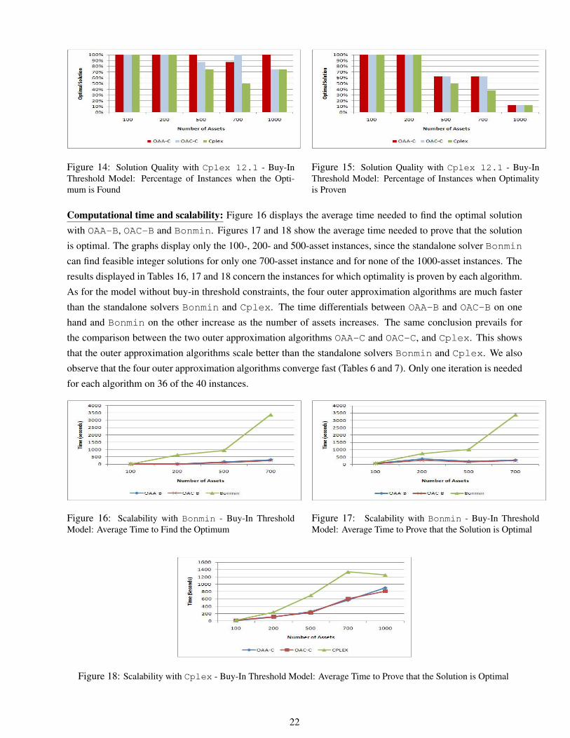
Figure 14: Solution Quality with Cplex 12.1 - Buy-InThreshold Model: Percentage of Instances when the Opti-mum is Found

Figure 15: Solution Quality with Cplex 12.1 - Buy-InThreshold Model: Percentage of Instances when Optimalityis Proven

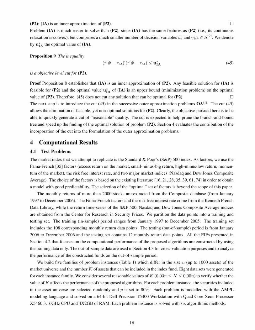
Computational time and scalability: Figure 16 displays the average time needed to find the optimal solution

with OAA-B, OAC-B and Bonmin. Figures 17 and 18 show the average time needed to prove that the solution

is optimal. The graphs display only the 100-, 200- and 500-asset instances, since the standalone solver Bonmin

can find feasible integer solutions for only one 700-asset instance and for none of the 1000-asset instances. The

results displayed in Tables 16, 17 and 18 concern the instances for which optimality is proven by each algorithm.

As for the model without buy-in threshold constraints, the four outer approximation algorithms are much faster

than the standalone solvers Bonmin and Cplex. The time differentials between OAA-B and OAC-B on one

hand and Bonmin on the other increase as the number of assets increases. The same conclusion prevails for

the comparison between the two outer approximation algorithms OAA-C and OAC-C, and Cplex. This shows

that the outer approximation algorithms scale better than the standalone solvers Bonmin and Cplex. We also

observe that the four outer approximation algorithms converge fast (Tables 6 and 7). Only one iteration is needed

for each algorithm on 36 of the 40 instances.

Figure 16: Scalability with Bonmin - Buy-In ThresholdModel: Average Time to Find the Optimum

Figure 17: Scalability with Bonmin - Buy-In ThresholdModel: Average Time to Prove that the Solution is Optimal

Figure 18: Scalability with Cplex - Buy-In Threshold Model: Average Time to Prove that the Solution is Optimal

22

Table 3 reports the average optimality (AOG) and integrality (AIG) gaps (in %) with the six methods. The

notation ∞ indicates that no representative gap measure could be obtained. The average optimality and inte-

grality gaps obtained with the standalone solvers Bonmin and Cplex are systematically larger than the ones

obtained with the outer approximation algorithms OAA-B, OAC-B, OAA-C and OAC-C.

Table 3: Average Optimality and Integrality Gaps (in %) - Buy-In Threshold ModelOAA-B OAC-B Bonmin OAA-C OAC-C Cplex

Number of Assets AOG AIG AOG AIG AOG AIG AOG AIG AOG AIG AOG AIG

100 0.00 0.00 0.00 0.00 0.00 0.00 0.00 0.00 0.00 0.00 0.00 0.00200 0.00 0.00 0.00 0.00 0.08 0.30 0.00 0.00 0.00 0.00 0.00 0.00500 0.02 0.15 0.02 0.15 0.09 0.28 0.00 0.12 0.00 0.13 0.06 0.29700 0.02 0.29 0.01 0.27 ∞ ∞ 0.00 0.20 0.00 0.18 0.02 0.37

1000 0.05 0.19 0.03 0.17 ∞ ∞ 0.00 0.19 0.01 0.22 0.02 0.26

The above analysis shows the versatility of the proposed outer approximation methods. The outer approxi-

mation algorithms OAA-B, OAC-B, OAA-C and OAC-C have been successfully applied to solve problem (PB)that includes buy-in threshold constraints. The problem (PB) with buy-in threshold constraints contains a larger

number of integer constraints and poses additional combinatorial challenges than problems (P1) and (P2) for

which the four algorithms were designed.

4.3 Analysis of Constructed Enhanced Index FundsThe proposed approach is intended to construct EIFs that perform well in-sample (i.e., on the data used for their

construction), and, most importantly, out-of-sample, as one moves from the period used in their construction.

For each problem instance, we use the index fund built on the basis of the in-sample period only (see Section

4.2) and verify how it performs on the one-year out-of-sample period.

Cross-Validation: The objective pursued in this study is to construct EIFs that closely track the S&P 500 index

while limiting the investors’ overall risk exposure. To verify whether these objectives are attained during the

out-of-sample period whose data were not used for the construction of the EIFs, we carry two types of cross-

validation experiments. The first one pertains to the tracking error and whether the EIFs and the S&P 500 index

share similar return patterns. The second experiment concerns the market risk exposure. More precisely, we

check whether the EIFs’ variance over the out-of-sample period is smaller than the maximum allowable variance

level υ that is probabilistically enforced with the constraint (5).

First, in order to analyze how closely the constructed EIFs follow the S&P 500 index, we use standard

statistical hypothesis tests. The null hypothesis of the tests is that the monthly return tracking error between the

S&P 500 index and each constructed EIF is 0. In other words, it means that on average there is no difference

between the monthly returns of the S&P 500 index and those of the considered EIF. Columns 2 to 11 in Tables

8 and 9 (for the model with buy-in constraints) report the p-value associated with each hypothesis test. The

p-value is the probability of wrongly rejecting the null hypothesis if it is in fact true. A small p-value indicates

that the null hypothesis is unlikely to be true: the smaller the p-value, the more reason one has to reject the null

hypothesis. The p-value is compared to the actual significance level of the test which we set at the level (5%)

usually used. Clearly, the null hypothesis according to which the EIF closely tracks the S&P 500 index is rejected

if the p-value is strictly smaller than 0.05.

For the in-sample period, for which we have 108 data points, we use the t-test. Columns named “IN” in

Tables 8 and 9 show the p-value of the tests concerning the in-sample period. Not surprisingly, one can observe

that the p-value is above 0.05 for each EIF and we do not reject the null hypothesis.

23

Next, we use the out-of-sample data points to cross-validate our approach and to check whether the con-

structed EIFs track closely the S&P 500 index on the out-of-sample period. Since the out-of-sample period

covers year 2006 and only contains 12 data points, it is not reasonable to employ the t-test. Hence, we use the

Wilcoxon sign rank test for the out-of-sample period. It is a non-parametric test analogue to the t-test that does

not require any assumptions about the distribution of the variable under consideration. Columns named “OUT”

in Tables 8 and 9 report the p-value for each test concerning the out-of-sample period. It can be seen that the null

hypothesis is rejected for only one instance (100-7). This confirms that our models permit the construction of

EIFs that closely track the S&P 500 index on (future) periods whose data were not used for the derivation of the

model. The result is even more significant considering that we never rebalance the constructed EIFs. The EIFs

are constructed on the basis on the 9-year in-sample period. They track well the S&P 500 index over that period

and continue doing so over the next year, without any rebalancing. Also, note that the asset universe for the 40

problem instances was constructed completely randomly. For each problem instance, we selected at random a

number (n=100, 200, 500, 700, 1000) of assets out of the 2000 assets for which we had the necessary data for

the period 1995-2006. In some problem instances, there was not a single asset included in the S&P 500 index

over the period 1995-2006.

Second, we evaluate whether the stochastic constraint (5) is actually effective for constructing risk-averse

EIFs. Recall that we impose that the EIFs variance must be smaller than υ = 0.005 with probability 90%.

Columns 12-16 in Tables 8 and 9 (for the buy-in threshold model) report the variance of the EIFs over the out-

of-sample period. Our risk averse-objective is clearly attained. The variance of each of the 80 EIFs is strictly

smaller (i.e., the largest value is 0.0017) than the threshold of 0.005.

Performance: After having shown that the constructed EIFs permit a close tracking of the S&P 500 index while

incurring a low overall variance, we shall now study the adjusted risk performance of the constructed EIFs. This

is accomplished by comparing the Sharpe ratio [84] of the EIFs with the Sharpe ratio of the S&P 500 index. The

Sharpe ratio is calculated by subtracting the risk-free rate from the return of a portfolio and dividing the result by

the standard deviation of the portfolio returns. It allows the verification of whether the portfolio’s returns are due

to good investment decisions or a result of excessive risk. An asset allocation is typically considered good if the

(possibly high) returns it generates do not come with too much additional risk. The Sharpe ratio is a key metric

to provide further insight into the performance of the constructed risk-averse EIFs. The Sharpe ratio of 97.5% of

the constructed EIFs exceeds the Sharpe ratio of the S&P 500 index fund.

5 ConclusionIndex fund allocation strategies have become increasingly popular due to the attractive return levels and the low

transaction and rebalancing costs they incur. We propose a new model for the pursuit of a risk-averse enhanced

indexation strategy and develop a new mathematical programming method based on the outer approximation

concept. The method involves the early detection of the problem structure and develops a hierarchical organiza-

tion of the computations with expanding sets of integer-restricted variables.

The proposed model constructs an index fund that mimics the return behavior of a benchmark market index.

It implements a risk-averse partial replication strategy that limits the market risk incurred by the investor. The

model takes into account the parameter estimation risk. We define asset returns and the return covariance terms

as random variables, which implies that the variance of the index fund is itself a random variable. No proba-

bilistic assumption is made on the asset returns that are driven by a set of factors whose return is stochastic. The

risk-averse feature limits the return variability of the index fund. Our model includes a probabilistic constraint

24

that prevents the variance of the index fund return from exceeding a specified risk threshold with a large prob-

ability level. The motivation for this comes from the existing literature [7, 29, 49, 77] which reports that it is

possible to design semi-active asset allocation strategies that reproduce very accurately the performance level of

a benchmark, but at the cost of a sometimes high overall variance. Not only does the risk-averse feature limit

the entailed market risk, but it also reduces the extent of a moral hazard problem related to the wage structure

of fund managers [49]. Indeed, the remuneration of fund managers often includes a performance fee component

[49], in which the salary is positively associated with the assumed risk [41, 49]. The risk constraint prevents the

managers from constructing highly volatile EIFs and acts as a covenant.

The risk-averse EIF model takes the form of a stochastic integer programming problem that cannot be solved

with any optimization solver in it original formulation. We propose two reformulation approaches to make the

above problem computationally tractable. The first approach consists in the derivation of a new deterministic

equivalent formulation for the stochastic constraint limiting the variance of the index fund. The second approach

resides in the application of a block decomposition method that provides a much sparser representation of the

VC matrix. This contributes to a significant decrease in computational times. The solution method involves

the construction of increasingly tighter outer approximation problems obtained through the relaxation of the

cardinality constraint and of the integrality restrictions on the binary variables associated with a carefully selected

subset of assets. A variant of the proposed approach that involves the generation of an objective level optimality

cut is also assessed.

We evaluate the performance of the outer approximation framework on 40 problem instances in which the

EIF tracks the S&P 500 index. The computational study shows that the outer approximation algorithm converges

in a very small number (1 or 2) of iterations, and allows to solve very efficiently complex problem instances in

which up to 1000 securities are considered for inclusion in the index fund. The strength of the obtained results

is highlighted when linked to recent statements claiming that “traditional optimization techniques cannot deal

appropriately with the discontinuities and the many local optima emerging from the introduction of explicit car-

dinality constraints” [66], or that exact methods “often cannot deal with the problem” [55] (i.e., index problem

with asset universe comprising between 100 and 600 securities). Moreover, the algorithmic framework is general

enough to allow the fast and optimal solution of problems including additional integer constraints, called buy-in

threshold trading constraints, which prevent from holding small positions. The proposed approach outperforms

the MINLP solvers Bonmin and Cplex 12.1 in terms of robustness (percentage of instances solved to opti-

mality) and computational times, and scales much better. The conclusions apply to the two types of models (i.e.,

with or without buy-in threshold constraint) and are even more marked for the more combinatorially involved

models including buy-in threshold constraints. The out-of-sample computational experiments show that the con-

structed EIFs track very closely the S&P 500 index fund benchmark over periods whose data were not used for

constructing the EIFs. More remarkable is that this result is obtained without any rebalancing operation over the

entire (10-year) period. It is also shown that the EIFs expose the investors to a much smaller market risk than

the one of the S&P 500 index and that the variance of each of the EIF over the out-of-sample period is strictly

smaller than the imposed threshold. More than 97% of the constructed EIFs generate a risk-adjusted return (i.e.,

Sharpe ratio) that is higher than the one of the S&P 500 index.

Note that the same algorithmic technique could be applied if the fund manager is required to invest in a mini-

mal number of assets. Future research will study the inclusion of transaction costs and of other trading constraints

(turnover, etc.), as well as the inclusion of a constraint requiring the generation of a higher return level than the

one of the benchmark (another form of enhanced indexation). Other algorithmic techniques involving, for exam-

25

ple, the polyhedral description of the continuous non-linear constraints or the derivation of lower objective level

feasibility cuts will also be studied. Another objective is to consider non-normally distributed factor returns.

References[1] K. Abhishek, S. Leyffer, and J. Linderoth. Filmint: An outer-approximation-based solver for nonlinear

mixed integer programs. INFORMS Journal of Computing, forthcoming, 2010.

[2] C. Alexander and A. Dimitriu. Index and statistical arbitrage: Tracking error or cointegration? Journal ofPortfolio Management, 31:50–63, 2005.

[3] J. Baskin, R. Ginis, and S. Schoenfeld. Finding the right blend of alpha and beta. Northern Trust WhitePaper, pages 1–4, 2005.

[4] V. S. Bawa, S. J. Brown, and R. W. Klein. Estimation Risk and Optimal Portfolio Choice. North-Holland,Amsterdam, The Netherlands, 1979.

[5] J. E. Beasley, N. Meade, and T.-J. Chang. An evolutionary heuristic for the index tracking problem. Euro-pean Journal of Operational Research, 148:621–643, 2003.

[6] P. Belotti. COUENNE, an open-source solver for mixed-integer non-convex problems. Working Paper,2009.

[7] P. Bertrand. Risk-adjusted performance attribution and portfolio optimisations under tracking-error con-straints. Journal of Asset Management, 10:75–88, 2009.

[8] D. Bertsimas, C. Darnell, and R. Soucy. Portfolio construction through mixed-integer programmming atGraham, Mayo, Van Otterloo and Company. Interfaces, 29:49–66, 1999.

[9] D. Bienstock. Computational study of a family of mixed-integer quadratic programming problems. Math-ematical Programming, 75:121–140, 1996.

[10] D. Blanchett. Can indexes generate alpha? Journal of Indexes, March/April:1–6, 2010.

[11] T. Bodnar and W. Schmid. The distribution of the sample variance of the global minimum variance portfolioin elliptical models. Statistics, 41(1):65–75, 2007.

[12] J. Bonafede. The Wilshire 5000 total market index: The logistics behind managing the U.S. stock market.Journal of Indexes, Third Quarter:1–5, 2003.

[13] P. Bonami, L. T. Biegler, A. R. Conn, G. Cornuejols, I. E. Grossmann, C. D. Laird, J. Lee, A. Lodi,F. Margot, N. Sawaya, and A. Wachter. An algorithmic framework for convex mixed integer nonlinearprograms. Discrete Optimization, 5:186–204, 2008.

[14] P. Bonami, M. Kılınc, and J. Linderoth. Algorithms and software for convex mixed integer nonlinearprograms. Working Paper, 2009.

[15] P. Bonami and M. A. Lejeune. An exact solution approach for portfolio optimization problems understochastic and integer constraint. Operations Research, 57(3):650–670, 2009.

[16] B. G. Briner and G. Connor. How much structure is best? A comparison of market model, factor modeland unstructured equity covariance matrices. The Journal of Risk, 10(4):3–30, 2008.

[17] M. Broadie. Computing efficient frontiers using estimated parameters. Annals of Operations Research,45:21–58, 1993.

[18] N. A. Canakgoz and J. E. Beasley. Mixed-integer programming approaches for index tracking and enhancedindexation. European Journal of Operational Research, 196(1):384–399, 2009.

[19] S. Ceria and R. A. Stubbs. Incorporating estimation errors into portfolio selection: Portfolio construction.Journal of Asset Management, 7(2):109–127, 2006.

[20] L. K. Chan, K. Jason, and J. Lakonishok. On portfolio optimization: Forecasting covariances and choosingthe risk model. The Review of Financial Studies, 12(5):937–974, 1999.

[21] T.-J. Chang, N. Meade, and Y. M. Shraiha. Heuristics for cardinality constrained portfolio optimisation.Computers and Operations Research, 27:1271–1302, 2000.

26

[22] L. Chavez-Bedoya and J. Birge. Index tracking and enhanced indexation using a parametric approach.Working Paper, pages 1–57, 2009.

[23] V. Chopra and W. T. Ziemba. The effects of errors in means, variances, and covariances on optimal portfoliochoice. Journal of Portfolio Management, 19:6–11, 1993.

[24] G. Chow. Portfolio selection based on return, risk and relative performance. Financial Analysts Journal,March-April:54–60, 1995.

[25] T. Coleman, Y. Li, and J. Henniger. Minimizing tracking error while restricting the number of assets. TheJournal of Risk, 8:33–56, 2006.

[26] G. Connor. The three types of factor models: A comparison of their explanatory power. Financial AnalystsJournal, May-June:42–46, 1995.

[27] G. Connor and R. Korajczyk. Factor models of asset returns. In S. Cont, editor, Encyclopedia of Quantita-tive Finance. Chicester, Wiley, 2010.

[28] F. Corielli and M. Marcellino. Factor based index tracking. Journal of Banking and Finance, 30:2215–2233,2006.

[29] G. Cornuejols and R. Tutuncu. Optimization Methods in Finance. Cambridge University Press, 2007.

[30] A. Corvalan. Mixed tactical asset allocation. Working Paper, 323:1–13, 2005.

[31] R. Dembo and D. Rosen. The practice of portfolio replication, a practical overview of forward and inverseproblems. Annals of Operations Research, 85:267–284, 1999.

[32] U. Derigs and N. Nickel. Meta-heuristic based decision support for portfolio optimization with a case studyon tracking error minimization in passive portfolio management. OR Spectrum, 25:345–378, 2003.

[33] C. Dose and S. Cincotti. Clustering of financial time series with application to index and enhanced trackingportfolio. Physica A, 355:154–151, 2005.

[34] M. Duran and I. E. Grossmann. An outer-approximation algorithm for a class of mixed integer nonlinearprograms. Mathematical Programming, 36, 1986.

[35] E. F. Fama and K. R. French. Common risk factors in the returns on stocks and bonds. Journal of FinancialEconomics, 33:3–56, 1993.

[36] R. Fletcher and S. Leyffer. Solving mixed integer nonlinear programs by outer approximation. Mathemat-ical Programming, 66:327–349, 1994.

[37] S. Focardi and F. Fabozzi. A methodolgy for inex tracking based on time-series clustering. QuantitativeFinance, 4:417–425, 2004.

[38] A. A. Gaivoronski, S. Krylov, and N. van der Wijst. Optimal portfolio selection and dynamic benchmarktracking. European Journal of Operational Research, 163:115–131, 2005.

[39] D. Goldfarb and G. Iyengar. Robust portfolio selection problems. Mathematics of Operations Research,28(1):1–38, 2003.

[40] M. Grinblatt and S. Titman. Adverse risk incentives and the design of performance-based contracts. Man-agement Science, 35(7):807–822, 1989.

[41] R. Grinold and A. Rudd. Incentive fees: Who wins? Who loses? Financial Analysts Journal, January-February:27–38, 1987.

[42] B. V. Halldorsson and R. H. Tutuncu. An interior-point method for a class of saddle point problems. Journalof Optimization Theory and Applications, 116(3):559–590, 2003.

[43] N. J. Higham. Computing the nearest correlation matrix - A problem from finance. IMA Journal of Numer-ical Analysis, 22:329–343, 2002.

[44] Investment Company Institute. 2009 Investment Company Fact Book - 49th edition, 2009, Washington,DC.

[45] B. I. Jacobs, K. N. Levy, and H. M. Markowitz. Portfolio optimization with factors, scenarios, and realisticshort positions. Operations Research, 53(4):586–599, 2005.

27

[46] R. Jansen and R. van Dijk. Optimal benchmark tracking with small portfolios. Journal of Portfolio Man-agement, 28:33–39, 2002.

[47] N. J. Jobst, M. D. Horniman, C. A. Lucas, and G. Mitra. Computational aspects of alternative portfolioselection models in the presence of discrete asset choice constraint. Quantitave Finance, 1:1–13, 2001.

[48] P. Jorion. Enhanced index funds and tracking error optimization. Working Paper, pages 1–26, 2002.

[49] P. Jorion. Portfolio optimization with tracking-error constraint. Financial Analysts Journal,September/October:70–82, 2003.

[50] S. Kataoka. A stochastic programming model. Econometrica, 31(1-2):181–196, 1963.

[51] H. Kellerer, R. Mansini, and M. G. Speranza. Selecting portfolios with fixed costs and minimum transactionlots. Annals of Operations Research, 99:287–304, 2000.

[52] J. Knight and S. Satchell. Linear Factor Models in Finance. Elsevier, Quantitative Finance Series, 2005.

[53] H. Konno and T. Hatagi. Index-plus-alpha tracking under concave transaction cost. Journal of Industrialand Management Optimization, 1(1):87–99, 2005.

[54] R. Kozlowski. Index managers see assets increase for first time since 2007:http://www.investmentnews.com/article/20090927/reg/309279975. Pensions & In-vestments Report, 2009.

[55] T. Krink, S. Mittnik, and S. Paterlini. Differential evolution and combinatorial search for constrained index-tracking. Annals of Operations Research, 171:153–176, 2009.

[56] M. A. Lejeune. A VAR Black-Litterman model for the construction of absolute return fund-of-funds.Quantitative Finance, Forthcoming, 2010.

[57] S. Leyffer. Generalized outer approximation. Encyclopedia of Optimization, 2:247–254, 2001.

[58] D. Li, X. Sun, and J. Wang. Convergent lagrangian method for separable integer programming: Objectivelevel cut and domain cut methods. In J. K. Karlof, editor, Integer Programming: Theory and Practice,pages 19–37. Taylor & Francis Group, Boca Raton, FL, 2006.

[59] D. Li, J. Wang, and X. Sun. Computing exact solution method to nonlinear integer programming: Conver-gent lagrangian and objective level cut method. Journal of Global Optimization, 39:127–154, 2007.

[60] J. Loftus. Enhanced equity indexing. In F. Fabozzi and R. Molay, editors, Perspectives on Equity Indexing,pages 83–84. Frank J. Fabozzi Associates, New Hope, PA, 2000.

[61] Z. Lu. A computational study on robust portfolio selection based on a joint ellipsoidal uncertainty set.Mathematical Programming, Forthcoming, 2010.

[62] D. Luenberger. Investment Science. Oxford University Press, 1998.

[63] D. C. Maley. Index Mutual Funds: How to Simplify Your Financial Life and Beat the Pro’s. ArtephiusPublishing, 1999.

[64] B. G. Malkiel. Passive investment strategies and efficient markets. European Financial Management,9(1):1–10, 2003.

[65] R. Mansini and M. G. Speranza. Heuristic algorithms for the portfolio selection problem with minimumtransaction lots. European Journal of Operational Research, 114:219–233, 1999.

[66] D. Maringer and O. Oyewumi. Index tracking with constrained portfolios. Intelligent Systems in Account-ing, Finance and Management, 15:57–71, 2007.

[67] H. Markowitz and A. F. Perold. Portfolio analysis with factors and scenarios. Journal of Finance, 36:871–877, 1981.

[68] H. M. Markowitz and E. V. Dijk. Risk-return analysis. In S. Zenios and W. Ziemba, editors, Handbookof Asset and Liability Management - Volume 1: Theory and Methodology, pages 139–197. North-Holland,2006.

[69] N. Meade and G. R. Salkin. Index funds - Construction and performance measurement. Journal Opera-tional Research Society, 40(10):871–879, 1989.

28

[70] R. C. Merton. On estimating the expected return on the market: An exploratory investigation. Journal ofFinancial Economics, 8:323–361, 1980.

[71] G. Miller. Equity risk modeling: A comparison of factor models. The MSCI Barra Newsletter, 181:2–17,2006.

[72] L. Mitra, G. Mitra, and D. Roman. Scenario generation for financial modelling: Desirable properties and acase study. OptiRisk Systems: White Paper Series, OPT 10:1–20, 2009.

[73] R. J. Muirhead. Aspects of Multivariate Statistical Theory. Wiley, New York, NY, 1982.

[74] A. F. Perold. Large-scale portfolio optimization. Management Science, 30(10):1143–1160, 1984.

[75] I. Quesada and I. Grossmann. An LP/NLP based branch and bound algorithm for convex MINLP optimiza-tion problems. Computers and Chemical Engineering, 16:937–947, 1992.

[76] B. Rafaely and J. Bennel. Optimisation of ftse 100 tracker funds. Managerial Finance, 32(6):447–492,2006.

[77] R. Roll. A mean/variance analysis of tracking error. The Journal of Portfolio Management, 18(4):13–22,1992.

[78] D. Rosen and D. Saunders. Analytical methods for hedging systematic credit risk with linear factor portfo-lios. Journal of Economic Dynamics & Control, 33:37–52, 2009.

[79] D. Rosen and D. Saunders. Risk factor contributions in portfolio credit risk models. Journal of Banking &Finance, 34(2):336–349, 2010.

[80] R. Ruiz-Torrubiano and A. Suarez. A hybrid optimization approach to index tracking. Annals of OperationsResearch, 166:57–71, 2009.

[81] S. Schoenfeld. Active Index Investing. John Wiley & Sons, Inc. Hoboken, NJ, 2004.

[82] S. Schoenfeld and J. Yang. Enhanced indexing: Adding index alpha in a disciplined, risk-controlled manner.In S. Schoenfeld, editor, Active Index Investing, pages 277–296. John Wiley & Sons. Hoboken, NY, 2004.

[83] W. F. Sharpe. A simplified model for portfolio analysis. Management Science, 9:277–293, 1963.

[84] W. F. Sharpe. The Sharpe Ratio. Journal of Portfolio Management, 21(1):49–58, 1994.

[85] D. X. Shaw, S. Liu, and L. Kopman. Lagrangian relaxation procedure for cardinality-constrained portfoliooptimization. Optimization Methods and Software, 23(3):411–420, 2008.

[86] J. Siegel. Indexing your portfolio: The evolution of indices.http://finance.yahoo.com/columnist/article/futureinvest/6953, 2006.

[87] S. Stoyan and R. Kwon. A two-stage stochastic mixed-integer programming approach to the index trackingproblem. Optimization and Engineering, 11(2):247–275, 2010.

[88] Vanguard 500 Index Funds. Vanguard:https://personal.vanguard.com/us/funds/snapshot?fundid=0040&fundintext=int,2010.

[89] J. P. Vielma, S. Ahmed, and G. L. Nemhauser. A lifted linear programming branch-and-bound algorithmfor mixed integer conic quadratic programs. INFORMS Journal on Computing, 20:438–450, 2008.

[90] F. Williams. Indexing growth slows in last half of 2000. Pensions & Investments, 2001.

[91] K. Worzel, C. Vassiadou-Zeniou, and S. Zenios. Integrated simulation and optimization models for trackingindices of fixed-income securities. Operations Research, 42:223–232, 1998.

[92] L. Wu, S. Chou, C. Yang, and C. Ong. Enhanced index investing based on goal programming. Journal ofPortfolio Management, 33(3):49–56, 2007.

[93] D. Yao, S. Zhang, and X. Zhou. Tracking a financial benchmark with a few assets. Operations Research,54:232–246, 2006.

29

App

endi

xC

olum

n1

inTa

ble

4re

port

sth

ena

me

ofth

epr

oble

min

stan

ce.C

olum

n2

give

sth

eop

timal

obje

ctiv

efu

nctio

nva

lueZ

∗ .C

olum

n3

(res

p.,1

1an

d19

)sho

ws

the

best

obje

ctiv

eva

lueZ

foun

dw

ithOAA-B

(res

p.,OAC-B

andBonmin

).C

olum

n4

(res

p.,1

3an

d20

)re

port

sth

etim

eto

show

that

the

solu

tion

isop

timal

with

OAA-B

(res

p.,OAC-B

and

Bonmin

).Fo

rOAC-B

,the

time

inco

lum

n13

isth

esu

mof

the

times

need

ed(i

)to

deriv

eth

eop

timal

itycu

t(co

lum

n12

)an

d(i

i)to

show

that

the

solu

tion

isop

timal

.W

hen

the

optim

ality

gap

isno

tclo

sed

with

inon

eho

ur,t

heen

try

inth

eta

ble

read

s”>

3600

”.C

olum

n5

(res

p.,1

4an

d21

)ind

icat

esth

etim

eto

find

the

optim

also

lutio

nw

ithOAA-B

(res

p.,OAC-B

andBonmin

).Fo

rOAC-B

,col

umn

14re

port

sth

esu

mof

the

times

need

ed(i

)to

deriv

eth

eop

timal

itycu

t(co

lum

n12

)an

d(i

i)to

find

the

optim

also

lutio

n.W

hen

the

optim

also

lutio

nis

nota

ttain

edw

ithin

one

hour

,the

entr

yin

the

tabl

ere

ads

”>36

00”.

Col

umn

6(r

esp.

,15

and

22)

disp

lays

the

optim

ality

gapO

=(Z−Z

∗ )/Z

with

OAA-B

(res

p.,OAC-B

andBonmin

).T

hesy

mbo

l”*”

indi

cate

sth

atth

eop

timal

solu

tion

was

foun

d(O

=0)

.Col

umn

7(r

esp.

,16

and

23)g

ives

the

best

low

erbo

undZ

obta

ined

with

OAA-B

(res

p.,OAC-B

andBonmin

).W

eus

e”*

”to

indi

cate

that

the

optim

ality

gap

was

clos

edan

dth

usth

atZ

=Z

∗ ;C

olum

n8

(res

p.,1

7an

d24

)rep

orts

the

inte

gral

ityga

pI

=(Z−Z

)/Z

with

OAA-B

(res

p.,OAC-B

andBonmin

).T

hesy

mbo

l”*”

indi

cate

sth

atth

eop

timal

solu

tion

was

prov

en(I

=0)

;Col

umns

9an

d18

prov

ide

the

num

bero

fite

ratio

nsw

ithOAA-B

andOAC-B

.Col

umn

10re

port

sth

enu

mbe

rofs

mal

l(i.e

.,<

0.01

)pos

ition

sin

the

optim

alin

dex

fund

.The

acro

nym

NS

indi

cate

sth

atno

feas

ible

inte

gers

olut

ion

was

foun

d.A

llco

mpu

tatio

nalt

imes

are

inC

PUse

cond

s.C

olum

ns6,

8,15

,17,

22an

d24

repo

rtth

eop

timal

ityan

din

tegr

ality

gaps

inpe

rcen

ts.

Tabl

e4:

Com

puta

tiona

lRes

ults

forP

robl

ems

with

outB

uy-I

nT

hres

hold

Con

stra

ints

with

Bonmin

OA

A-B

OA

C-B

Bon

min

12

34

56

78

910

1112

1314

1516

1718

1920

2122

2324

100-

10.

207

0.20

74.

640.

98*

**

10

0.20

70.

75.

391.

65*

**

10.

207

9.22

4.61

**

*10

0-2

0.20

50.

205

4.75

1.26

**

*1

00.

205

0.97

5.67

2.16

**

*1

0.20

59.

74.

66*

**

100-

30.

201

0.20

18.

581.

58*

**

10

0.20

11.

349.

932.

89*

**

10.

201

12.7

74.

69*

**

100-

40.

194

0.19

46.

391.

23*

**

10

0.19

41.

147.

472.

36*

**

10.

194

10.4

44.

99*

**

100-

50.

196

0.19

682

.13

1.44

**

*2

00.

196

3.06

86.3

14.

51*

**

20.

196

455.

0642

6.09

**

*10

0-6

0.20

80.

208

230.

0790

.02

**

*2

00.

208

9.09

200.

441

.76

**

*2

0.20

811

5.39

29.6

6*

**

100-

70.

206

0.20

669

.34

5*

**

10

0.20

66.

5672

.42

10.7

8*

**

10.

206

>36

0034

68.5

8*

0.20

31.

2410

0-8

0.19

60.

196

5.08

1.16

**

*1

00.

196

0.78

4.01

1.91

**

*1

0.19

67.

194.

56*

**

200-

10.

190

0.19

074

.41

6.3

**

*1

20.

190

5.89

75.3

111

.84

**

*1

0.19

011

4.8

114.

5*

**

200-

20.

183

0.18

311

.66

4.73

**

*1

00.

183

0.53

11.8

4.76

**

*1

0.18

344

.45

44.1

4*

**

200-

30.

181

0.18

111

1.83

7.48

**

*1

00.

181

6.39

120.

6113

.53

**

*1

0.18

116

5.22

164.

95*

**

200-

40.

187

0.18

761

.75

6.22

**

*1

00.

187

3.5

65.6

49.

38*

**

10.

187

7877

.67

**

*20

0-5

0.19

20.

192

3249

.14

1285

.73

**

*2

00.

192

16.0

822

61.1

622

.96

**

*2

0.19

3>

3600

2647

.08

0.54

0.18

91.

720

0-6

0.19

20.

192

106.

817.

03*

**

10

0.19

24.

9189

.14

11.4

7*

**

10.

192

165.

1316

4.81

**

*20

0-7

0.19

60.

196

39.8

45.

86*

**

10

0.19

62.

542

.17

8.05

**

*1

0.19

677

.22

76.8

9*

**

200-

80.

180

0.18

058

3.19

6.78

**

*1

00.

180

32.2

859

0.12

38.7

8*

**

10.

180

864.

9786

4.83

**

*50

0-1

0.15

10.

151

>36

0039

0.96

0.04

0.15

00.

741

20.

151

6.41

>36

0021

36.4

10.

090.

150

0.74

10.

151

>36

0032

38.0

90.

290.

150

0.99

500-

20.

171

0.17

112

8.31

75.5

3*

**

15

0.17

13.

0911

8.39

63.1

4*

**

10.

171

525.

8146

7.31

**

*50

0-3

0.15

40.

154

68.1

463

.72

**

*1

60.

154

2.89

56.1

756

.17

**

*1

0.15

441

240

5.03

**

*50

0-4

0.17

80.

178

128.

9278

.98

**

*1

60.

178

3.31

109.

6563

.54

**

*1

0.17

852

6.38

469.

22*

**

500-

50.

156

0.15

6>

3600

82.6

7*

0.15

6*

14

0.15

651

.92

>36

0012

3.36

*0.

155

0.49

10.

156

>36

0085

8.86

00.

156

0.3

500-

60.

157

0.15

716

1.95

71.8

6*

**

16

0.15

72.

8114

2.31

58.6

1*

**

10.

157

589.

3448

3.31

**

*50

0-7

0.14

30.

143

>36

0021

49.1

40.

110.

143

0.11

11

0.14

315

.3>

3600

1612

.99

0.11

0.14

20.

581

0.14

3>

3600

470.

760.

160.

142

0.9

500-

80.

157

0.15

782

.03

63.5

2*

**

17

0.15

73

68.1

749

.78

**

*1

0.15

750

2.94

502.

94*

**

700-

10.

139

0.13

9>

3600

209.

03*

0.13

80.

961

30.

139

13.3

6>

3600

209.

69*

0.13

80.

811

0.14

0>

3600

2576

.97

0.15

0.13

80.

9270

0-2

0.15

30.

153

181.

3815

7.81

**

*1

60.

153

7.42

186.

0616

2.87

**

*1

0.15

314

88.8

114

88.8

1*

**

700-

30.

166

0.16

616

6.44

164.

25*

**

15

0.16

67.

712

3.7

121.

54*

**

10.

166

1389

.41

1387

.7*

**

700-

40.

134

0.13

4>

3600

3555

.92

0.09

0.13

31.

061

00.

134

8.11

>36

0035

86.7

3*

0.13

30.

971

0.13

4>

3600

2087

.41

0.1

0.13

30.

7770

0-5

0.15

30.

153

178.

6417

6.58

**

*1

70.

153

7.31

121.

3111

9.26

**

*1

0.15

313

73.1

313

71.4

4*

**

700-

60.

154

0.15

416

3.81

163.

81*

**

16

0.15

47.

5911

3.61

113.

61*

**

10.

154

1394

.38

1394

.38

**

*70

0-7

0.16

30.

163

804.

4220

5.2

**

*1

40.

163

7.05

775.

6817

3.05

**

*1

0.16

320

44.1

414

25.5

6*

**

700-

80.

139

0.13

936

0119

7.69

0.04

0.13

81.

061

30.

139

6.88

>36

0019

1.2

0.04

0.13

80.

951

0.13

9>

3600

1993

.27

0.04

0.13

80.

9510

00-1

0.12

80.

128

>36

0053

8.09

*0.

128

0.23

12

0.12

820

.13

>36

0046

9.51

*0.

128

0.23

1N

S>

3600

NS

NS

NS

NS

1000

-20.

145

0.14

556

4.39

492.

45*

**

18

0.14

516

.38

441.

9636

8.69

**

*1

NS

>36

00N

SN

SN

SN

S10

00-3

0.13

00.

130

>36

0034

95.1

40.

050.

130

0.13

13

0.13

012

.57

>36

0087

5.79

0.04

0.13

00.

131

NS

>36

00N

SN

SN

SN

S10

00-4

0.12

70.

128

>36

0033

22.8

40.

230.

127

0.74

13

0.12

818

.28

>36

0050

1.06

0.24

0.12

60.

851

NS

>36

00N

SN

SN

SN

S10

00-5

0.14

60.

146

972.

3655

0.66

**

*1

100.

146

16.2

377

0.73

376.

12*

**

1N

S>

3600

NS

NS

NS

NS

1000

-60.

124

0.12

4>

3600

503.

280.

040.

124

0.16

15

0.12

410

.23

>36

0061

0.97

0.04

0.12

40.

161

NS

>36

00N

SN

SN

SN

S10

00-7

0.15

80.

158

>36

0053

8.38

*0.

157

0.15

15

0.15

820

.06

>36

0047

5.01

*0.

157

0.15

1N

S>

3600

NS

NS

NS

NS

1000

-80.

131

0.13

1>

3600

1603

.84

*0.

130

0.09

15

0.13

115

.72

>36

0016

13.8

3*

0.13

00.

091

NS

>36

00N

SN

SN

SN

S

30

Tabl

e5:

Com

puta

tiona

lRes

ults

forP

robl

ems

with

outB

uy-I

nT

hres

hold

Con

stra

ints

with

Cplex12.1

OA

A-C

OA

C-C

Cpl

ex1

23

46

78

911

1213

1516

1718

1920

2223

2410

0-1

0.20

70.

207

6.89

1*

**

10.

207

0.70

7.39

**

*1

0.20

78.

88*

**

100-

20.

205

0.20

55.

406

**

*1

0.20

50.

976.

67*

**

10.

205

7.89

**

*10

0-3

0.20

10.

201

7.73

4*

**

10.

201

1.34

9.51

**

*1

0.20

116

.20

**

*10

0-4

0.19

40.

194

6.64

1*

**

10.

194

1.14

7.80

**

*1

0.19

49.

88*

**

100-

50.

196

0.19

627

.594

**

*2

0.19

63.

0629

.86

**

*2

0.19

639

.95

**

*10

0-6

0.20

80.

208

41.3

9*

**

20.

208

9.09

50.0

9*

**

20.

208

66.0

9*

**

100-

70.

206

0.20

613

.203

**

*1

0.20

66.

5619

.56

**

*1

0.20

646

.25

**

*10

0-8

0.19

60.

196

6.25

**

*1

0.19

60.

787.

14*

**

10.

196

5.61

**

*20

0-1

0.19

00.

190

32.8

29*

**

10.

190

5.89

25.9

2*

**

10.

190

43.1

6*

**

200-

20.

183

0.18

385

.635

**

*1

0.18

30.

5383

.83

**

*1

0.18

320

4.13

**

*20

0-3

0.18

10.

181

75.4

22*

**

10.

181

6.39

79.5

2*

**

10.

181

219.

73*

**

200-

40.

187

0.18

732

.173

**

*2

0.18

73.

5024

.45

**

*2

0.18

748

.52

**

*20

0-5

0.19

20.

192

208.

609

**

*1

0.19

216

.08

220.

00*

**

10.

192

351.

56*

**

200-

60.

192

0.19

235

.891

**

*1

0.19

24.

9139

.80

**

*1

0.19

272

.72

**

*20

0-7

0.19

60.

196

35.4

69*

**

10.

196

2.50

36.0

9*

**

10.

196

86.5

2*

**

200-

80.

180

0.18

027

7.15

7*

**

10.

180

32.2

829

8.08

**

*1

0.18

091

3.81

**

*50

0-1

0.15

10.

151

>36

00*

0.15

10.

241

0.15

16.

41>

3600

*0.

151

0.24

10.

151

>36

000.

050.

1500

0.69

500-

20.

171

0.17

117

0.79

8*

**

10.

171

3.09

175.

20*

**

10.

171

403.

14*

**

500-

30.

154

0.15

486

.485

**

*1

0.15

42.

8964

.53

**

*1

0.15

522

1.20

**

*50

0-4

0.17

80.

178

121.

219

**

*1

0.17

83.

3111

8.72

**

*1

0.17

823

6.63

**

*50

0-5

0.15

60.

156

2019

.16

**

*1

0.15

651

.92

1956

.44

**

*1

0.15

621

57.5

2*

**

500-

60.

157

0.15

716

3.89

1*

**

10.

157

2.81

206.

03*

**

10.

157

340.

42*

**

500-

70.

143

0.14

3>

3600

0.03

0.14

20.

311

0.14

315

.30

>36

000.

030.

142

0.31

10.

143

>36

000.

360.

1420

0.78

500-

80.

157

0.15

714

3.18

7*

**

10.

157

3.00

135.

72*

**

10.

157

165.

39*

**

700-

10.

139

0.14

0>

3600

0.09

0.13

90.

591

0.14

013

.36

>36

000.

120.

139

0.61

10.

140

>36

000.

170.

1384

0.88

700-

20.

153

0.15

320

9.26

5*

**

10.

153

7.42

287.

36*

**

10.

153

164.

19*

**

700-

30.

166

0.16

618

1.73

3*

**

10.

166

7.70

182.

84*

**

10.

166

191.

38*

**

700-

40.

134

0.13

4>

3600

*0.

134

0.31

10.

134

8.11

>36

00*

0.13

40.

381

0.13

4>

3600

*0.

1334

0.61

700-

50.

153

0.15

327

4.03

2*

**

10.

153

7.31

152.

80*

**

10.

153

206.

80*

**

700-

60.

154

0.15

416

0.85

9*

**

10.

154

7.59

127.

38*

**

10.

154

109.

38*

**

700-

70.

164

0.16

467

8.43

8*

**

10.

164

7.05

732.

83*

**

10.

164

1062

.03

**

*70

0-8

0.13

90.

139

>36

00*

0.13

90.

441

0.13

96.

88>

3600

*0.

139

0.44

10.

139

>36

000.

010.

1383

0.60

1000

-10.

128

0.12

818

96.4

2*

**

10.

128

20.1

318

52.6

5*

**

10.

128

>36

00*

0.12

770.

2910

00-2

0.14

50.

145

539.

781

**

*1

0.14

516

.38

389.

13*

**

10.

145

1025

.00

**

*10

00-3

0.13

00.

130

823.

906

**

*1

0.13

012

.57

682.

86*

**

10.

130

1160

.39

**

*10

00-4

0.12

70.

127

>36

000.

040.

127

0.47

10.

127

18.2

8>

3600

*0.

127

0.43

10.

128

>36

000.

260.

1265

0.84

1000

-50.

146

0.14

691

4.37

5*

**

10.

146

16.2

391

0.67

**

*1

0.14

617

06.0

3*

**

1000

-60.

124

0.12

424

61.9

5*

**

10.

124

10.2

324

05.6

7*

**

10.

124

>36

000.

050.

1243

0.05

1000

-70.

158

0.15

832

00.3

6*

**

10.

158

20.0

634

52.2

5*

**

10.

158

>36

000.

040.

1575

0.04

1000

-80.

131

0.13

126

16.3

9*

**

10.

131

15.7

226

72.5

9*

**

10.

131

>36

000.

250.

1305

0.48

31

Tabl

e6:

Com

puta

tiona

lRes

ults

forP

robl

ems

with

Buy

-In

Thr

esho

ldC

onst

rain

tsw

ithBonmin

OA

A-B

OA

C-B

Bon

min

12

34

56

78

911

1213

1415

1617

1819

2021

2223

2410

0-1

0.20

70.

207

7.34

1.75

**

*1

0.20

70.

527.

302.

18*

**

10.

207

28.4

212

.89

**

*10

0-2

0.20

50.

205

10.1

92.

53*

**

10.

205

0.39

6.83

2.78

**

*1

0.20

521

.11

4.16

**

*10

0-3

0.20

10.

201

11.6

62.

75*

**

10.

201

1.25

13.0

23.

80*

**

10.

201

38.1

75.

92*

**

100-

40.

194

0.19

47.

581.

88*

**

10.

194

1.13

8.32

2.76

**

*1

0.19

417

.98

3.36

**

*10

0-5

0.19

60.

196

126.

032.

42*

**

20.

196

2.30

121.

834.

61*

**

20.

196

143.

099.

42*

**

100-

60.

208

0.20

825

2.14

92.9

9*

**

20.

208

3.69

223.

0578

.60

**

*1

0.20

830

8.70

112.

69*

**

100-

70.

206

0.20

682

.03

5.03

**

*1

0.20

62.

2065

.73

6.50

**

*2

0.20

612

3.08

16.1

4*

**

100-

80.

196

0.19

64.

501.

86*

**

10.

196

0.45

4.64

2.20

**

*1

0.19

617

.50

10.2

2*

**

200-

10.

190

0.19

013

1.88

15.2

2*

**

10.

190

0.84

123.

7213

.76

**

*1

0.19

047

3.88

473.

88*

**

200-

20.

183

0.18

315

.55

1.45

**

*1

0.18

30.

3014

.11

9.02

**

*1

0.18

389

.64

74.5

6*

**

200-

30.

181

0.18

115

2.80

24.3

1*

**

10.

181

2.56

148.

2825

.20

**

*1

0.18

120

37.6

120

12.1

6*

**

200-

40.

187

0.18

710

4.34

11.2

5*

**

10.

187

1.58

105.

2111

.28

**

*1

0.18

739

1.59

391.

59*

**

200-

50.

192

0.19

217

48.5

912

.03

**

*2

0.19

22.

3811

99.3

014

.30

**

*3

0.19

212

44.2

073

7.33

0.21

0.19

01.

1020

0-6

0.19

20.

192

94.8

815

.25

**

*1

0.19

23.

1710

1.48

17.4

5*

**

1N

SN

SN

SN

SN

SN

S20

0-7

0.19

60.

196

75.8

431

.55

**

*1

0.19

61.

3051

.00

12.3

8*

**

10.

196

223.

9876

.31

**

*20

0-8

0.18

00.

180

596.

729.

69*

**

10.

180

12.3

659

5.66

22.1

9*

**

10.

181

>36

0029

03.5

30.

370.

179

0.97

500-

10.

151

0.15

1>

3600

390.

960.

040.

150

0.74

10.

151

6.41

>36

0021

36.4

10.

090.

150

0.74

10.

151

>36

0032

38.0

90.

290.

150

0.99

500-

20.

171

0.17

115

7.83

147.

27*

**

10.

171

0.84

139.

3412

8.31

**

*1

0.17

110

51.9

510

47.6

4*

**

500-

30.

155

0.15

512

7.03

127.

03*

**

10.

155

0.58

95.3

193

.24

**

*1

0.15

591

1.77

911.

77*

**

500-

40.

178

0.17

833

2.69

251.

39*

**

10.

178

0.95

248.

4713

0.76

**

*1

0.17

815

17.1

313

37.1

4*

**

500-

50.

156

0.15

627

69.9

865

9.30

**

*1

0.15

62.

1418

75.1

444

3.94

**

*1

0.15

7>

3600

1679

.38

0.12

0.15

60.

4350

0-6

0.15

80.

158

197.

1716

2.66

**

*1

0.15

80.

6116

2.45

136.

53*

**

10.

158

1241

.58

1188

.14

**

*50

0-7

0.14

30.

143

>36

0023

56.5

00.

090.

142

0.48

10.

143

3.53

>36

0022

19.7

20.

050.

142

0.44

10.

143

>36

0022

79.6

70.

320.

142

0.85

500-

80.

157

0.15

719

7.74

120.

77*

**

10.

157

0.83

140.

4210

0.80

**

*1

0.15

732

6.83

235.

97*

**

700-

10.

139

0.13

9>

3600

521.

61*

0.13

80.

771

0.13

93.

20>

3600

490.

14*

0.13

80.

771

NS

>36

00N

SN

SN

SN

S70

0-2

0.15

30.

153

500.

0948

0.19

**

*1

0.15

30.

5038

0.75

242.

81*

**

1N

S>

3600

NS

NS

NS

NS

700-

30.

166

0.16

629

3.45

293.

45*

**

10.

166

0.53

255.

8725

5.87

**

*1

0.16

633

85.8

133

85.8

1*

**

700-

40.

134

0.13

4>

3600

624.

940.

010.

133

0.78

10.

134

6.42

>36

0020

88.6

50.

050.

133

0.71

1N

S>

3600

NS

NS

NS

NS

700-

50.

153

0.15

344

1.63

237.

45*

**

10.

153

0.58

334.

2827

1.81

**

*1

NS

>36

00N

SN

SN

SN

S70

0-6

0.15

40.

154

248.

1421

7.11

**

*1

0.15

40.

4125

0.25

200.

75*

**

1N

S>

3600

NS

NS

NS

NS

700-

70.

164

0.16

451

4.56

468.

63*

**

10.

164

0.92

367.

0625

3.58

**

*1

NS

>36

00N

SN

SN

SN

S70

0-8

0.13

90.

139

>36

0023

84.1

60.

110.

138

0.76

10.

139

77.5

8>

3600

2380

.27

*0.

138

0.71

1N

S>

3600

NS

NS

NS

NS

1000

-10.

128

0.12

8>

3600

1963

.33

0.11

0.12

80.

361

0.12

82.

44>

3600

833.

10*

0.12

80.

291

NS

>36

00N

SN

SN

SN

S10

00-2

0.14

50.

145

1124

.97

1076

.41

**

*1

0.14

51.

0285

1.25

793.

35*

**

1N

S>

3600

NS

NS

NS

NS

1000

-30.

130

0.13

0>

3600

1208

.36

*0.

130

0.08

10.

130

1.14

>36

0088

3.23

*0.

130

0.08

1N

S>

3600

NS

NS

NS

NS

1000

-40.

127

0.12

8>

3600

860.

360.

210.

127

0.83

10.

128

15.7

2>

3600

667.

200.

240.

127

0.87

1N

S>

3600

NS

NS

NS

NS

1000

-50.

146

0.14

621

11.3

110

32.1

1*

**

10.

146

0.91

3219

.44

844.

64*

**

1N

S>

3600

NS

NS

NS

NS

1000

-60.

125

0.12

514

03.6

411

78.4

1*

**

10.

125

1.14

1286

.95

829.

87*

**

1N

S>

3600

NS

NS

NS

NS

1000

-70.

158

0.15

8>

3600

1443

.88

0.04

0.15

80.

121

0.15

81.

52>

3600

1557

.63

*0.

158

0.06

1N

S>

3600

NS

NS

NS

NS

1000

-80.

131

0.13

1>

3600

1308

.91

0.02

0.13

10.

111

0.13

10.

81>

3600

1490

.51

*0.

131

0.09

1N

S>

3600

NS

NS

NS

NS

32

Tabl

e7:

Com

puta

tiona

lRes

ults

forP

robl

ems

with

Buy

-In

Thr

esho

ldC

onst

rain

tsw

ithCplex12.1

OA

A-C

OA

C-C

Cpl

ex1

23

46

78

911

1213

1516

1718

1920

2223

2410

0-1

0.20

680.

2068

7.05

**

*1

0.20

70.

708.

14*

**

10.

207

9.30

**

*10

0-2

0.20

470.

2047

6.69

**

*1

0.20

50.

977.

87*

**

10.

205

7.75

**

*10

0-3

0.20

110.

2011

9.36

**

*1

0.20

11.

3410

.14

**

*1

0.20

116

.21

**

*10

0-4

0.19

360.

1936

6.69

**

*1

0.19

41.

148.

94*

**

10.

194

9.72

**

*10

0-5

0.19

640.

1964

27.8

1*

**

20.

196

3.06

32.8

6*

**

20.

196

36.5

9*

**

100-

60.

2076

0.20

7648

.16

**

*2

0.20

89.

0961

.08

**

*2

0.20

866

.53

**

*10

0-7

0.20

580.

2058

13.9

7*

**

10.

206

6.56

21.3

3*

**

10.

206

45.5

6*

**

100-

80.

1958

0.19

586.

12*

**

10.

196

0.78

7.48

**

*1

0.19

66.

03*

**

200-

10.

1902

0.19

0234

.81

**

*1

0.19

05.

8934

.00

**

*1

0.19

043

.16

**

*20

0-2

0.18

300.

1830

89.8

3*

**

10.

183

0.53

93.0

3*

**

10.

183

204.

13*

**

200-

30.

1808

0.18

0879

.30

**

*1

0.18

16.

3986

.47

**

*1

0.18

121

8.59

**

*20

0-4

0.18

660.

1866

24.4

7*

**

10.

187

3.50

34.6

3*

**

10.

187

48.5

2*

**

200-

50.

1917

0.19

1723

6.42

**

*2

0.19

216

.08

257.

53*

**

20.

192

351.

56*

**

200-

60.

1921

0.19

2134

.39

**

*1

0.19

24.

9142

.06

**

*1

0.19

272

.72

**

*20

0-7

0.19

640.

1964

34.8

0*

**

10.

196

2.50

40.0

3*

**

10.

196

85.7

8*

**

200-

80.

1804

0.18

0429

1.48

**

*1

0.18

032

.28

343.

33*

**

10.

180

906.

22*

**

500-

10.

1511

0.15

11>

3600

*0.

150

0.61

10.

151

6.41

>36

00*

0.15

00.

611

0.15

1>

3600

0.04

0.15

00.

7950

0-2

0.17

090.

1709

103.

63*

**

10.

171

3.09

127.

73*

**

10.

171

654.

22*

**

500-

30.

1548

0.15

4820

6.11

**

*1

0.15

52.

8918

1.47

**

*1

0.15

438

2.69

**

*50

0-4

0.17

800.

1780

1610

.77

**

*1

0.17

83.

3115

66.7

2*

**

10.

178

>36

00*

0.17

80.

3050

0-5

0.15

630.

1563

>36

00*

0.15

60.

081

0.15

651

.92

>36

00*

0.15

60.

081

0.15

6>

3600

*0.

156

0.40

500-

60.

1575

0.15

7544

2.23

**

*1

0.15

82.

8136

4.89

**

*1

0.15

811

63.0

6*

**

500-

70.

1426

0.14

26>

3600

*0.

142

0.3

10.

143

15.3

0>

3600

0.02

0.14

20.

321

0.14

3>

3600

0.40

0.14

20.

8450

0-8

0.15

680.

1568

268.

70*

**

10.

157

3.00

244.

38*

**

10.

157

583.

61*

**

700-

10.

1395

0.13

96>

3600

0.03

0.13

90.

711

0.14

013

.36

>36

00*

0.13

90.

61

0.14

0>

3600

0.05

0.13

90.

7970

0-2

0.15

310.

1531

2270

.20

**

*1

0.15

37.

4221

40.2

5*

**

10.

153

>36

000.

020.

153

0.18

700-

30.

1663

0.16

6341

4.20

**

*1

0.16

67.

7041

6.27

**

*1

0.16

625

5.59

**

*70

0-4

0.13

430.

1343

>36

00*

0.13

40.

421

0.13

48.

11>

3600

*0.

134

0.42

10.

134

>36

000.

110.

133

0.76

700-

50.

1534

0.15

3421

70.5

5*

**

10.

153

7.31

2120

.23

**

*1

0.15

3>

3600

*0.

153

0.15

700-

60.

1545

0.15

4543

6.16

**

*1

0.15

47.

5961

1.45

**

*1

0.15

494

3.69

**

*70

0-7

0.16

360.

1636

851.

53*

**

10.

164

7.05

792.

72*

**

10.

164

2811

.19

**

*70

0-8

0.13

910.

1391

>36

00*

0.13

90.

451

0.13

96.

88>

3600

*0.

139

0.45

10.

139

>36

000.

010.

138

0.74

1000

-10.

1282

0.12

82>

3600

*0.

128

0.06

10.

128

20.1

3>

3600

*0.

128

0.06

10.

128

>36

00*

0.12

80.

1310

00-2

0.14

540.

1454

>36

00*

0.14

50.

311

0.14

516

.38

>36

00*

0.14

50.

311

0.14

5>

3600

*0.

145

0.24

1000

-30.

1301

0.13

0190

4.87

**

*1

0.13

012

.57

814.

54*

**

10.

130

1252

.34

**

*10

00-4

0.12

740.

1274

>36

00*

0.12

70.

441

0.12

718

.28

>36

000.

050.

127

0.50

10.

128

>36

000.

130.

127

0.73

1000

-50.

1462

0.14

62>

3600

*0.

146

0.17

20.

146

16.2

3>

3600

*0.

146

0.17

20.

146

>36

00*

0.14

60.

1010

00-6

0.12

450.

1245

>36

00*

0.12

40.

111

0.12

510

.23

>36

00*

0.12

40.

111

0.12

5>

3600

*0.

124

0.19

1000

-70.

1577

0.15

77>

3600

*0.

158

0.13

10.

158

20.0

6>

3600

*0.

158

0.13

10.

158

>36

00*

0.15

70.

1910

00-8

0.13

110.

1311

>36

00*

0.13

10.

271

0.13

115

.72

>36

000.

020.

131

0.45

10.

131

>36

000.

040.

131

0.46

33

Tabl

e8:

Perf

orm

ance

ofC

onst

ruct

edE

nhan

ced

Inde

xFu

nds

-Mod

elw

ithou

tBuy

-in

Thr

esho

ldC

onst

rain

tsN

umbe

rofA

sset

s10

020

050

070

010

0010

020

050

070

010

00

Dat

aSe

tSi

gnifi

canc

eL

evel

Out

-of-

Sam

ple

Peri

odR

etur

nV

aria

nce

INO

UT

INO

UT

INO

UT

INO

UT

INO

UT

10.

3590

0.10

800.

8790

0.12

600.

1690

0.84

500.

1400

0.90

600.

1350

0.78

400.

0002

0.00

010.

0017

0.00

120.

0009

20.

4280

0.10

800.

7260

0.22

400.

3760

0.45

600.

0830

0.55

600.

0670

0.78

400.

0001

0.00

020.

0003

0.00

050.

0007

30.

6030

0.10

800.

6750

0.22

400.

1380

0.78

400.

4530

0.45

600.

1010

0.90

600.

0002

0.00

030.

0006

0.00

030.

0013

40.

3540

0.09

200.

7910

0.06

500.

6580

0.17

000.

1810

0.96

900.

0870

0.50

500.

0001

0.00

020.

0003

0.00

120.

0011

50.

4860

0.22

400.

8250

0.07

800.

3790

0.96

900.

2940

0.50

500.

0920

0.90

600.

0007

0.00

030.

0004

0.00

110.

0008

60.

4960

0.10

800.

9990

0.14

700.

2420

0.90

600.

0760

0.66

600.

0780

0.55

600.

0001

0.00

020.

0016

0.00

050.

0010

70.

7420

0.03

100.

8650

0.55

600.

2210

0.84

500.

5810

0.41

000.

3020

0.72

400.

0001

0.00

020.

0012

0.00

040.

0004

80.

9120

0.10

800.

9320

0.12

600.

2000

0.78

400.

1400

0.78

400.

1500

0.41

000.

0002

0.00

020.

0005

0.00

130.

0004

Tabl

e9:

Perf

orm

ance

ofC

onst

ruct

edE

nhan

ced

Inde

xFu

nds

-Mod

elw

ithB

uy-i

nT

hres

hold

Con

stra

ints

Num

bero

fAss

ets

100

200

500

700

1000

100

200

500

700

1000

Dat

aSe

tSi

gnifi

canc

eL

evel

Out

-of-

Sam

ple

Peri

odR

etur

nV

aria

nce

INO

UT

INO

UT

INO

UT

INO

UT

INO

UT

10.

3590

0.10

800.

8790

0.12

600.

2110

0.61

000.

1250

0.72

400.

1410

0.72

400.

0002

0.00

010.

0016

0.00

120.

0009

20.

4280

0.10

800.

7510

0.19

600.

3800

0.55

600.

0790

0.61

000.

0590

1.00

000.

0001

0.00

020.

0003

0.00

050.

0008

30.

6030

0.10

800.

6760

0.22

400.

1390

0.84

500.

4700

0.41

000.

1060

0.90

600.

0002

0.00

030.

0006

0.00

030.

0012

40.

3540

0.09

200.

7920

0.06

500.

6400

0.14

700.

1950

1.00

000.

0780

0.41

000.

0001

0.00

020.

0002

0.00

120.

0011

50.

4860

0.22

400.

7960

0.10

800.

3410

0.90

600.

2650

0.61

000.

0970

0.96

900.

0007

0.00

020.

0004

0.00

100.

0007

60.

4960

0.10

800.

9990

0.14

700.

2160

0.96

900.

0770

0.90

600.

0600

0.61

000.

0001

0.00

020.

0016

0.00

060.

0011

70.

7430

0.03

100.

8650

0.55

600.

2420

0.84

500.

4410

0.45

600.

1650

0.72

400.

0001

0.00

020.

0011

0.00

040.

0004

80.

9120

0.10

800.

9320

0.12

600.

1870

0.78

400.

1400

0.78

400.

1490

0.25

500.

0002

0.00

020.

0005

0.00

130.

0004

34