Embed Size (px)
Citation preview

EE365: Risk Averse Control
Risk averse optimization
Exponential risk aversion
Risk averse control
1

Risk averse optimization
2

Risk measures
I suppose f is a random variable we’d like to be small(i.e., an objective or cost)
I E f gives average or mean value
I many ways to quantify risk (of a large value of f)
I Prob(f ≥ fbad) (value-at-risk, VAR)
I E(f − fbad)+ (conditional value-at-risk, CVAR)
I var f = E(f −E f)2 (variance)
I E(f −E f)2+ (downside variance)
I Eφ(f), where φ is increasing and convex(when large f is good: expected utility EU(f) with increasing concaveutility function U)
I risk aversion: we want E f small and low risk
3

Risk averse optimization
I now suppose random cost f(x, ω) is a function of a decision variable x and arandom variable ω
I different choices of x lead to different values of mean cost E f(x, ω) and riskR(f(x, ω))
I there is typically a trade-off between minimizing mean cost and risk
I standard approach: minimize E f(x, ω) + λR(f(x, ω))
I E f(x, ω) + λR(f(x, ω)) is the risk-adjusted mean cost
I λ > 0 is called the risk aversion parameter
I varying λ over (0,∞) gives trade-off of mean cost and risk
I mean-variance optimization: choose x to minimize E f(x, ω)+λvar f(x, ω)
4

Example: Stochastic shortest path
I find path in directed graph from vertex A to vertex B
I edge weights are independent random variables with known distributions
I commit to path beforehand, with no knowledge of weight values
I path length L is random variable
I minimize EL+ λvarL, with λ ≥ 0
I for fixed λ, reduces to deterministic shortest path problem with edge weightsEwe + λvarwe
5

Stochastic shortest path
1
2
3
4
5
6
7
8
(7, 40)
(14, 3)
(5, 22)
(9, 35)
(7, 23)
(8, 2)
(1, 5)
(8, 125)
(6, 12)
(11, 8)
(4, 9)
(6, 200)
(8, 8)
(7, 12)
I find path from vertex A = 1 to vertex B = 8
I edge weights are lognormally distributed
I edges labeled with mean and variance: (Ewe,varwe)
6

Stochastic shortest path
λ = 0: EL = 30, varL = 400
1
2
3
4
5
6
7
8
(7, 40)
(14, 3)
(5, 22)
(9, 35)
(7, 23)
(8, 2)
(1, 5)
(8, 125)
(6, 12)
(11, 8)
(4, 9)
(6, 200)
(8, 8)
(7, 12)
7

Stochastic shortest path
λ = 0.05: EL = 35, varL = 100
1
2
3
4
5
6
7
8
(7, 40)
(14, 3)
(5, 22)
(9, 35)
(7, 23)
(8, 2)
(1, 5)
(8, 125)
(6, 12)
(11, 8)
(4, 9)
(6, 200)
(8, 8)
(7, 12)
8

Stochastic shortest path
λ = 10: EL = 40, varL = 25
1
2
3
4
5
6
7
8
(7, 40)
(14, 3)
(5, 22)
(9, 35)
(7, 23)
(8, 2)
(1, 5)
(8, 125)
(6, 12)
(11, 8)
(4, 9)
(6, 200)
(8, 8)
(7, 12)
9

Stochastic shortest path
trade-off curve: λ = 0, λ = 0.05, λ = 10
10

Stochastic shortest path
distribution of L: λ = 0, λ = 0.05, λ = 10
11
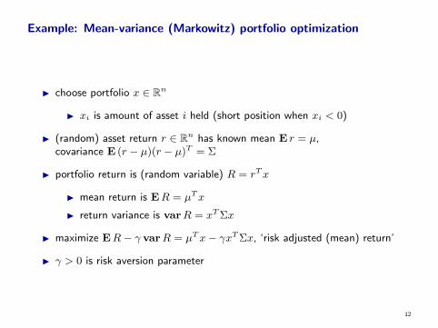
Example: Mean-variance (Markowitz) portfolio optimization
I choose portfolio x ∈ Rn
I xi is amount of asset i held (short position when xi < 0)
I (random) asset return r ∈ Rn has known mean E r = µ,covariance E (r − µ)(r − µ)T = Σ
I portfolio return is (random variable) R = rTx
I mean return is ER = µTx
I return variance is varR = xTΣx
I maximize ER− γ varR = µTx− γxTΣx, ‘risk adjusted (mean) return’
I γ > 0 is risk aversion parameter
12

Example: Mean-variance (Markowitz) portfolio optimization
I can add constraints such as
I 1Tx = 1 (budget constraint)
I x ≥ 0 (long positions only)
I can be solved as a (convex) quadratic program (QP)
maximize µTx− γxTΣxsubject to 1Tx = 1, x ≥ 0
(or analytically without long-only constraint)
I varying γ gives trade-off of mean return and risk
13
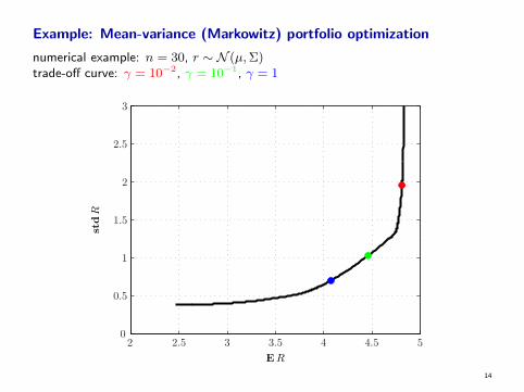
Example: Mean-variance (Markowitz) portfolio optimization
numerical example: n = 30, r ∼ N (µ,Σ)trade-off curve: γ = 10−2, γ = 10−1, γ = 1
14

Example: Mean-variance (Markowitz) portfolio optimization
numerical example: n = 30, r ∼ N (µ,Σ)distribution of portfolio return: γ = 10−2, γ = 10−1, γ = 1
15

Exponential risk aversion
16

Exponential risk aversion
I suppose f is a random variable
I exponential risk measure, with parameter γ > 0, is given by
Rγ(f) =1
γlog (E exp(γf))
(Rγ(f) =∞ if f is heavy-tailed)
I exp(γf) term emphasizes large values of f
I Rγ(f) is (up to a factor of γ) the cumulant generating function of f
I we haveRγ(f) = E f + (γ/2)var f + o(γ)
I so minimizing exponential risk is (approximately) mean-variance optimization,with risk aversion parameter γ/2
17
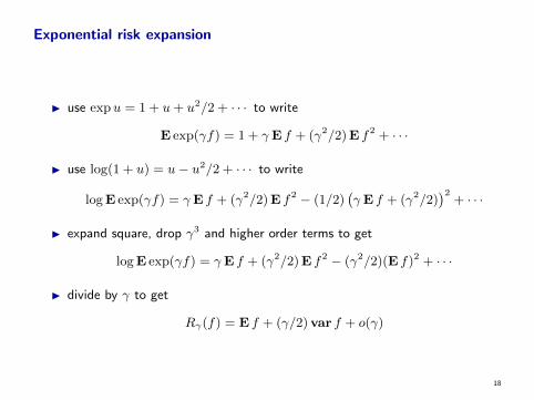
Exponential risk expansion
I use expu = 1 + u+ u2/2 + · · · to write
E exp(γf) = 1 + γE f + (γ2/2)E f2 + · · ·
I use log(1 + u) = u− u2/2 + · · · to write
logE exp(γf) = γE f + (γ2/2)E f2 − (1/2)(γE f + (γ2/2)
)2+ · · ·
I expand square, drop γ3 and higher order terms to get
logE exp(γf) = γE f + (γ2/2)E f2 − (γ2/2)(E f)2 + · · ·
I divide by γ to get
Rγ(f) = E f + (γ/2)var f + o(γ)
18

Properties
I Rγ(f) = E f + (γ/2)var f for f normal
I Rγ(a+ f) = a+Rγ(f) for deterministic a
I Rγ(f) can be thought of as a variance adjusted mean, but in fact it’s probablycloser to what you really want (e.g., it penalizes deviations above the meanmore than deviations below)
I monotonicity: if f ≤ g, then Rγ(f) ≤ Rγ(g)
I can extend idea to conditional expectation:
Rγ(f | g) =1
γlogE(exp(γf) | g)
19

Value at risk bound
I exponential risk gives an upper bound on VaR (value at risk)
I indicator function of f ≥ fbad is Ibad(f) =
{0 f < fbad
1 f ≥ fbad
I E Ibad(f) = Prob(f ≥ fbad)
I for γ > 0, exp γ(f − fbad) ≥ Ibad(f) (for all f)
I so E exp γ(f − fbad) ≥ E Ibad(f)
I henceProb(f ≥ fbad) ≤ exp γ(Rγ(f)− fbad)
20

Risk averse control
21

Risk averse stochastic control
I dynamics: xt+1 = ft(xt, ut, wt), with x0, w0, w1, . . . independent
I state feedback policy: ut = µt(xt), t = 0, . . . , T − 1
I risk averse objective:
J =1
γlogE exp γ
(T−1∑t=0
gt(xt, ut) + gT (xT )
)
I gt is stage cost; gT is terminal cost
I γ > 0 is risk aversion parameter
I risk averse stochastic control problem:find policy µ = (µ0, . . . , µT−1) that minimizes J
22

Interpretation
I total cost is random variable
C =
T−1∑t=0
gt(xt, ut) + gT (xT )
I standard stochastic control minimizes EC
I risk averse control minimizes Rγ(C)
I risk averse policy yields larger expected total cost than standard policy, butsmaller risk
23

Risk averse value function
I we are to minimize
J = Rγ
(T−1∑t=0
gt(xt, ut) + gT (xT )
)
over policies µ = (µ0, . . . , µT−1)
I define value function
Vt(x) = minµt,...,µT−1
Rγ
(T−1∑τ=t
gτ (xτ , uτ ) + gT (xT )
∣∣∣∣∣ xt = x
)
I VT (x) = gT (x)
I could minimize over input ut, policies µt+1, . . . , µT−1
I same as usual value function, but replace E with Rγ
24

Risk averse dynamic programming
I optimal policy µ? is
µ?t (x) ∈ argminu
(gt(x, u) +RγVt+1(ft(x, u, wt)))
where expectation in Rγ is over wt
I (backward) recursion for Vt:
Vt(x) = minu
(gt(x, u) +RγVt+1(ft(x, u, wt)))
I same as usual DP, but replace E with Rγ (both over wt)
25

Multiplicative version
I precompute ht(x, u) = exp γgt(x, u)
I instead of Vt, change variables Wt(x) = exp γVt(x)
I DP recursion is
Wt(x) = minu
(ht(x, u)EWt+1(ft(x, u, wt))
)I optimal policy is
µ?t (x) ∈ argminu
(ht(x, u)EWt+1(ft(x, u, wt))
)
26

Example: Optimal purchase
I must buy an item in one of T = 4 time periods
I prices are IID with p2t uniformly distributed on {1, . . . , 10}
I in each time period, the price is revealed and you choose to buy or wait
I once you’ve bought the item, your only option is to wait
I in the last period, you must buy the item if you haven’t already
27

Example: Optimal purchase
optimal policy: wait, buy
1 2 3 4
1
2
3
4
5
6
7
8
9
10
pt
t
γ → 0
1 2 3 4
1
2
3
4
5
6
7
8
9
10
pt
t
γ = 1
1 2 3 4
1
2
3
4
5
6
7
8
9
10
pt
t
γ = 2
28

Example: Optimal purchase
distribution of purchase price: γ → 0, γ = 1, γ = 2
1 1.5 2 2.5 3 3.50
0.05
0.1
0.15
0.2
0.25
price
probability
29