Committee - Dynamic positioningdynamic-positioning.com/proceedings/dp2001/high_tech_cao.pdf · Return to Session Directory > Y. Cao et al, Stress Engineering Services High Tech Dynamic

Author’s Name Name of the Paper Session

PDynamic Positioning Committee

Marine Technology Society

DYNAMIC POSITIONING CONFERENCE September 18-19, 2001

HIGH TECH SESSION

Dynamic Positioning of Drilling Vessels with A Fuzzy Logic Controller

Yusong Cao

Stress Engineering Services, Inc. (Houston, TX, USA)

Tzung-hang Lee Tamkang University (Tamsui, Taiwan, R.O.C)

David L Garrett John F Chappell

Stress Engineering Services, Inc. (Houston, TX, USA)

Return to Session Directory >

Y. Cao et al, Stress Engineering Services High Tech Dynamic Positioning of Drilling Vessels With a Fuzzy Logic Controller

DP Conference, Houston September 18-19 1

ABSTRACT

In this paper, a fuzzy logic controller for dynamic positioning of drilling vessels in deep water is presented. The core of the fuzzy controller is a set of fuzzy associative memory (FAM) rules that correlate each group of fuzzy control input sets to a fuzzy control output set. A FAM rule is a logical if-then type statement based on one’s sense of realism and experience or can be provided by an expert operator. The design of the fuzzy controller is very simple and does not require mathematical modeling of the complicated nonlinear system based on first principles. The fuzzy controller uses measured vessel heading, yaw rate, distance and velocity of the vessel relative to the desired position (location and heading) to generate the control outputs to bring the vessel to and maintain it in the desired position. The control outputs include the rudder angle, propeller thrust and lateral bow thrust. The effectiveness and robustness of the fuzzy controller are demonstrated through numerical time-domain simulations of the dynamic positioning of a drill ship of Mariner Class hull with use of nonlinear ship equations of motions.

1. INTRODUCTION

Offshore drilling vessels are subject to complicated environmental disturbances. Station-

keeping of a vessel is required so that the vessel can maintain a position close to the desired location of operation. As exploration and production for natural resources in oceans get into deeper water, dynamic positioning (DP) of offshore drilling vessels is becoming increasingly important. DP uses available control devices (such as rudder, propeller and vector thrusters, etc.) to counteract the environmental forces and keeps the vessel as close as possible to the desired position. DP has many advantages over other conventional station-keeping methods, such as mooring lines, for deepwater operations (CMPT, 1998).

Dynamic positioning by an automatic controller, as compared to that by a human operator, can increase the efficiency for regular routine operations within the design limits. However, an experienced operator, under no adverse influence, such as fatigue, drug or alcohol, can perform better than a conventional automatic control system, especially in a complicated situation.

A conventional automatic controller, such a PID controller, uses a so-called white-box approach to acquire the knowledge about the system (or process) to be controlled. The philosophy of the white-box approach lies in that if the characteristics of all the elements in the box (representing the process being considered) are known, then the complete relation between the process output and input can be obtained. The white-box approach attempts to describe the elements in terms of mathematical formulae (models). Major drawbacks of the white-box approach are: 1) a good mathematical model depends on our knowledge about each of the elements in the system and unfortunately our knowledge about the elements is limited and incomplete most of time; and 2) even if we can develop an accurate mathematical model, our ability to solve the mathematical problem is limited. Assumptions and approximations about the physics of the process must be made to simplify the formulae so that a quick and reasonably accurate solution is possible. Therefore, in most situations, the knowledge acquired through the white-box approach is incomplete. The human operator, on the other hand, acquires the knowledge about the process using the so-called black-box approach. By observing enough input-output samples, the human operator is able to establish the relation between the input and output of the process using the brain neural computing and fuzzy reasoning and performs a very effective control. A controller using Artificial Neural Networks (ANN) attempts to mimic neural computing of the human being, while a controller based on Fuzzy Logic (FL) attempts to mimic a human being’s fuzzy reasoning. One of the advantages of ANN or FL controllers is that no mathematical modeling of the process based on first principles is necessary. A good overview of neural computing and fuzzy reasoning is given by Kosko (1992).


Y. Cao, et al, Stress Engineering Services High Tech Dynamic Positioning of Drilling Vessels with a Fuzzy Logic Controller

DP Conference, Houston September 18-19, 2001 2

Attempts have been made to develop ANN and FL controllers for marine vessels. Ishii, Fujii and Ura (1994) developed an adaptive controller based on ANN for autonomous underwater vehicles. Zhang, Hearn and Sen (1997a, 1997b) used the ANN approach to design course-keeping autopilots, track-keeping controllers and automatic berthing systems for ships. Gu, Pao and Yip (1993) and Li and Gu (1996) investigated a special neural network, the so-called functional-link network, for dynamic positioning of ships. Cao, Zhou and Vorus (2000) developed an on-line trained auto-regressive moving average function-link ANN predictor/controller for dynamic positioning of marine vessels. FL controllers have been applied to depth control of unmanned undersea vehicles (DeBitrtto, 1994) and to autopilot design (Robert, 1997). Fang and Chiou (2000) reported the use of a self-tuning fuzzy control for the motion simulation of a SWATH ship. Parsons, Chubb, and Cao (1995) conducted an assessment of fuzzy logic vessel path control for a class of relatively simple cases whose objective was to bring a ship from an initial offset and heading to a desired straight-line course (heading control) using the ship’s rudder. Cao and Lee (2001) extended the work by Parsons et al (1995) and developed a FL controller for the course-keeping, path-tracking and dynamic positioning of surface ships.

This paper applies the FL controller developed by Cao and Lee (2001) to the dynamic positioning of drill ships. The main difference in the dynamic positioning of a drill ship and a conventional ship is that the drill ship has a drilling riser attached to it. The drilling riser adds a significant complexity to the mathematical modeling of the coupled ship-riser system for the design of a conventional automatic DP controller. In this paper, however, we will show, through the numerical simulations, that the FL controller developed for conventional ships works for drill ships as well with little modification.

2. FUZZY LOGIC CONTROL

The core of a FL controller is a set of the fuzzy associative memory (FAM) rules that correlate a fuzzy input set to a fuzzy output set of the FL controller. These rules establish linguistically how the control output should vary with the control input. A FAM rule is a logical if-then type statement: such as “if these antecedent components (group of fuzzy inputs) occur then this consequence (fuzzy output) should be used”. Given a set of control inputs, the controller applies appropriate rules to generate a set of control outputs. The FAM rules can be derived based on one’s sense of realism, experience, and expert knowledge about the process. Fuzzy set and fuzzy logic theories are applied to quantify the control inputs, FAM rules and control outputs.

Usually, a human operator uses the differences (errors) between the system outputs and the desired values and the rates of changes in the errors as the antecedents to derive the consequence based on the knowledge (not necessarily very precise) about the process from the experience. This type of control strategy is very simple and generic. Effective control actions can be generated very quickly. Human beings have been using it effectively for a very wide range of processes or systems for a long time.

The process considered in this paper is the dynamic positioning of a drill ship in an environment with a mean current under the controlled actions of rudder angle Rδ , increase in

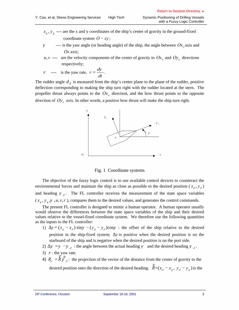
thrust of main propeller PT , and lateral bow thrust BT . Two coordinate systems (frames) are used to describe the motion of a drilling ship in the horizontal plane (see Fig. 1). Frame

oo yxO − is fixed at the center of gravity of the ship and Frame xyO − is the ground-fixed

coordinate system. With use of the concept of state space representation of a system, the position and orientation of the ship is uniquely determined by ( rvuyx gg ,,,,, ψ ) referred as the

state space variables. ( rvuyx gg ,,,,, ψ ) are defined as,




gg yx , ---- are the x and y coordinates of the ship’s center of gravity in the ground-fixed

coordinate system xyO − ;

ψ ---- is the yaw angle (or heading angle) of the ship, the angle between oOx axis and

Ox axis; vu, ---- are the velocity components of the center of gravity in oOx and oOy directions

respectively;

r ---- is the yaw rate, dt

dr

ψ= .

The rudder angle Rδ is measured from the ship’s center plane to the plane of the rudder, positive deflection corresponding to making the ship turn right with the rudder located at the stern. The propeller thrust always points to the oOx direction, and the bow thrust points to the opposite

direction of oOy axis. In other words, a positive bow thrust will make the ship turn right.

ψ

x

y

O

o

oy

ox

Fig. 1 Coordinate systems

The objective of the fuzzy logic control is to use available control devices to counteract the environmental forces and maintain the ship as close as possible to the desired position ( dd yx , )

and heading dψ . The FL controller receives the measurement of the state space variables

( rvuyx gg ,,,,, ψ ), compares them to the desired values, and generates the control commands.

The present FL controller is designed to mimic a human operator. A human operator usually would observe the differences between the state space variables of the ship and their desired values relative to the vessel-fixed coordinate system. We therefore use the following quantities as the inputs to the FL controller:

1) ψψ cos)(sin)( dgdg yyxxy −−−=∆ : the offset of the ship relative to the desired

position in the ship-fixed system; y∆ is positive when the desired position is on the starboard of the ship and is negative when the desired position is on the port side.

2) dψψψ −=∆ : the angle between the actual heading ψ and the desired heading dψ .

3) r : the yaw rate.

4) dRR ψψ

ρρ⋅= : the projection of the vector of the distance from the center of gravity to the

desired position onto the direction of the desired heading. ),( gdgd yyxxR −−=ρ

is the




distance vector from the center of gravity to the desired position; dψρ

is the unit vector in

the direction of the desired heading.

5) ||

)(RR

VVV gdd ϖ

ϖϖϖ

⋅−= : the projection of the relative velocity of the desired position to the

ship’s center of gravity onto the straight line from the center of gravity to the desired position. The quantity reflects how fast the ship approaches the desired point.

The above five quantities are normalized as,

LYy

y∆

=∆ , Lψψ

ψ∆

=∆ , Lrr

r = , LR

RR ψ

ψ = and L

dd V

VV = (1)

using corresponding scaling factors LY , Lψ , Lr , LR and LV whose values are to be chosen based

on particular process. Similarly, the three control outputs, Rδ , PT , and BT are normalized as,

,RL

RR δ

δδ =

PL

PP T

TT = ,

BL

BB T

TT = (2)

where RLδ , PLT , and BLT are scaling factors. The normalization makes the design of the FAM rules easier because it allows use of the same ranges of fuzzy sets and membership functions for different normalized inputs or outputs, and the outputs of similar effects may be derived using the same FAM rules. Another advantage of the normalization is that the same FL controller developed in the normalized space can be easily implemented in different vessels by applying the simple scaling factors. Therefore, the fuzzy control of the vessel will thereafter be dealt with in the normalized space for the rest of the paper.

To generate control commands, the FL controller proceeds through the following steps (Kosko 1992 and Parsons et al 1995):

1) Fuzzification

The FL controller first receives “crisp” numerical values of the measured states of the vessel, ( rvuyx gg ,,,,, ψ ), and computes ,,, ry ψ∆∆ ψR and dV . Each of the five

numerical inputs is assigned to linquistically described fuzzy sets defined over certain ranges. The number of fuzzy sets for each input (or output) is a matter of design. Kosko (1992) suggests the number of fuzzy sets be greater than three to avoid poor representation but less than nine to avoid unwarranted computational cost in practical applications.

We use seven fuzzy sets for ψ∆ . The seven fuzzy sets are: large negative (LN), medium negative (MN), small negative (SN), zero (ZE), small positive (SP), medium positive (MP), and large positive (LP). Similarly, we use five fuzzy sets for y∆ , five fuzzy

sets for r , seven fuzzy sets for ψR , and seven fuzzy sets for dV . These fuzzy sets are

defined in the ranges listed in Tables 1a – 1b.

Fuzzy sets

),,( dVRψψ∆

LN MN SN ZE SP MP LP

Range < -0.5 -0.6 to -0.2 -0.3 to 0.0 -0.1 to 0.1 0.0 to 0.3 0.2 to 0.6 > 0.5

Table 1a. Fuzzy set for ψ∆ , ψR and dV




Fuzzy sets ( y∆ and γ )

LN SN ZE SP LP

Range < -0.3 -0.5 to 0.0 -0.1 to 0.1 0.0 to 0.5 > 0.3

Table 1b. Fuzzy set for y∆ and γ

2) Assignment of Degrees of Membership Each of the five inputs is assigned a degree of membership in each of its linquistic

fuzzy sets. In designing the membership functions, the following guidelines are used: i) the number of fuzzy sets to which a crisp input can belong to should not exceed two. Thus, the input can only have non-zero degrees of membership in two adjacent fuzzy sets and degrees of memberships to other fuzzy sets are zero. ii) the degrees of membership in complementary fuzzy sets add to unity. iii) the membership function for each ZE fuzzy set has zero as its center. iv) membership functions near ( ,,, ry ψ∆∆ ψR , dV ) = (0, 0, 0, 0, 0) are narrower

than those farther from the desired values. This results in a finer regulator control. In our design, the normalized control inputs ψ∆ , ψR and dV have the same membership

functions (Fig.2), while y∆ and r have the same membership functions (Fig.3)

0

0 . 5

1 . 0

1 . 5

- 1 . 0 - 0 . 9 - 0 . 8 - 0 . 7 - 0 . 6 - 0 . 5 - 0 . 4 - 0 . 3 - 0 . 2 - 0 . 1 0 0 . 1 0 . 2 0 . 3 0 . 4 0 . 5 0 . 6 0 . 7 0 . 8 0 . 9 1 . 0

S P L PM PZ ES N M N L N

De

gre

e o

f m

emb

ers

hip

Fig. 2 Membership functions for ψ∆ ψR and dV

0

0 . 5

1 . 0

1 . 5

- 1 . 0 - 0 . 5 0 0 . 5 1 . 0

L PS PZ ES NL N

Deg

ree

of m

embe

rshi

p

Fig. 3 Membership functions for y∆ and r




3) Application of FAM Rules The FL controller correlates each group of fuzzy input sets to a group of fuzzy output

sets through a Fuzzy Associative Memory (FAM) rule. A FAM rule is a logical if-then statement: “if this antecedent (group of fuzzy input sets) occurs, then this consequent (group of fuzzy output sets) should be used”. The FL controller applies (“fires”) the FAM rules to each nonempty group of fuzzy input sets and generates a set of control action ( Rδ , pT , BT ).

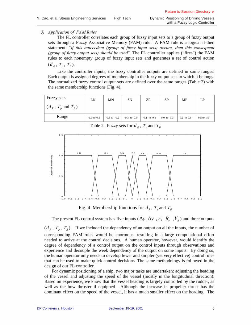
Like the controller inputs, the fuzzy controller outputs are defined in some ranges. Each output is assigned degrees of membership in the fuzzy output sets to which it belongs. The normalized fuzzy control output sets are defined over the same ranges (Table 2) with the same membership functions (Fig. 4).

Fuzzy sets

( Rδ , pT and BT )


Range -1.0 to-0.5 -0.6 to -0.2 -0.3 to 0.0 -0.1 to 0.1 0.0 to 0.3 0.2 to 0.6 0.5 to 1.0

Table 2. Fuzzy sets for Rδ , pT and BT

0

0 . 5

1 . 0

1 . 5

- 1 . 0 - 0 . 9 - 0 . 8 - 0 . 7 - 0 . 6 - 0 . 5 - 0 . 4 - 0 . 3 - 0 . 2 - 0 . 1 0 0 . 1 0 . 2 0 . 3 0 . 4 0 . 5 0 . 6 0 . 7 0 . 8 0 . 9 1 . 0

S P L PM PZ ES N M N L N

De

gre

e o

f m

em

be

rsh

ip

Fig. 4 Membership functions for Rδ , pT and BT

The present FL control system has five inputs ( ,,, ry ψ∆∆ ψR , dV ) and three outputs

( Rδ , pT , BT ). If we included the dependency of an output on all the inputs, the number of

corresponding FAM rules would be enormous, resulting in a large computational effort needed to arrive at the control decisions. A human operator, however, would identify the degree of dependency of a control output on the control inputs through observations and experience and decouple the week dependency of the output on some inputs. By doing so, the human operator only needs to develop fewer and simpler (yet very effective) control rules that can be used to make quick control decisions. The same methodology is followed in the design of our FL controller.

For dynamic positioning of a ship, two major tasks are undertaken: adjusting the heading of the vessel and adjusting the speed of the vessel (mostly in the longitudinal direction). Based on experience, we know that the vessel heading is largely controlled by the rudder, as well as the bow thruster if equipped. Although the increase in propeller thrust has the dominant effect on the speed of the vessel, it has a much smaller effect on the heading. The




rudder, as well as the bow thruster, has less effect on the speed of the vessel than the propeller. Therefore, we decouple the dependency of PT on ψ∆∆ ,y and r . The

dependency of the rudder and bow thruster on ψR and dV are also decoupled.

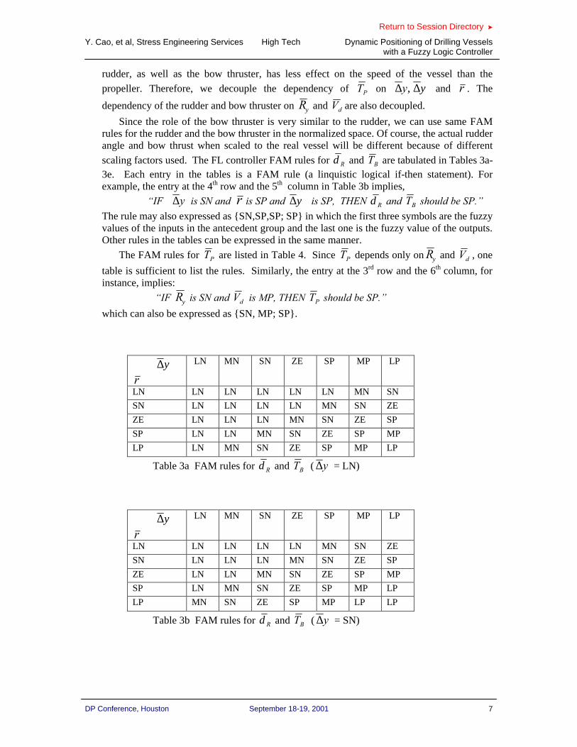
Since the role of the bow thruster is very similar to the rudder, we can use same FAM rules for the rudder and the bow thruster in the normalized space. Of course, the actual rudder angle and bow thrust when scaled to the real vessel will be different because of different scaling factors used. The FL controller FAM rules for Rδ and BT are tabulated in Tables 3a-3e. Each entry in the tables is a FAM rule (a linquistic logical if-then statement). For example, the entry at the 4th row and the 5th column in Table 3b implies,

“IF y∆ is SN and r is SP and ψ∆ is SP, THEN Rδ and BT should be SP.”

The rule may also expressed as {SN,SP,SP; SP} in which the first three symbols are the fuzzy values of the inputs in the antecedent group and the last one is the fuzzy value of the outputs. Other rules in the tables can be expressed in the same manner.

The FAM rules for PT are listed in Table 4. Since PT depends only on ψR and dV , one

table is sufficient to list the rules. Similarly, the entry at the 3rd row and the 6th column, for instance, implies:

“IF ψR is SN and dV is MP, THEN PT should be SP.”

which can also be expressed as {SN, MP; SP}.

ψ∆

r


LN LN LN LN LN LN MN SN

SN LN LN LN LN MN SN ZE

ZE LN LN LN MN SN ZE SP

SP LN LN MN SN ZE SP MP

LP LN MN SN ZE SP MP LP

Table 3a FAM rules for Rδ and BT ( y∆ = LN)

ψ∆

r


LN LN LN LN LN MN SN ZE

SN LN LN LN MN SN ZE SP

ZE LN LN MN SN ZE SP MP

SP LN MN SN ZE SP MP LP

LP MN SN ZE SP MP LP LP

Table 3b FAM rules for Rδ and BT ( y∆ = SN)




ψ∆

r


LN LN LN MN MN SN ZE SP

SN LN MN MN SN ZE SP MP

ZE MN MN SN ZE SP MP MP

SP MN SN ZE SP MP MP LP

LP SN ZE SP MP MP LP LP

Table 3c FAM rules for Rδ and BT ( y∆ = ZE)

ψ∆

r


LN LN LN MN SN ZE SP MP

SN LN MN SN ZE SP MP LP

ZE MN SN ZE SP MP LP LP

SP SN ZE SP MP LP LP LP

LP ZE SP MP LP LP LP LP

Table 3d FAM rules for Rδ and BT ( y∆ = SP)

ψ∆

r


LN LN MN SN ZE SP MP LP

SN MN SN ZE SP MP LP LP

ZE SN ZE SP MP LP LP LP

SP ZE SP MP LP LP LP LP

LP SP MP LP LP LP LP LP

Table 3e FAM rules for Rδ and BT ( y∆ = LP)

dV

ψR


LN LN LN LN LN MN SN ZE

MN LN LN LN MN SN ZE SP

SN LN LN MN SN ZE SP MP

ZE LN MN SN ZE SP MP LP

SP MN SN ZE SP MP LP LP

MP SN ZE SP MP LP LP LP

LP ZE SP MP LP LP LP LP

Table 4 FAM rules for PT




Notice that there are 224 FAM rules in total (175 rules for Rδ and BT , and 49 rules for

PT ). However, only 116 rules (88 rules for Rδ and BT , and 28 for PT ) need to be actually determined assuming symmetry of the vessel about the center plane.

4) Correlation-Minimum Inference Procedure

The degree to which a FAM rule is fired is determined by a so-called correlation-minimum inference procedure (Kosko 1992, Parsons et al 1995). For Rδ (or BT ), each group of the three input variable fuzzy sets has a corresponding degree of membership in that antecedent group. In the correlation-minimum inference procedure, the greatest degree of the membership that y∆ , ψ∆ and r have collectively in the conjunctive (i.e. AND) antecedent group is the smallest of the individual degrees of membership of the antecedent group’s components. This greatest degree is also called the degree to which the rule is fired. For example, if y∆ belongs to fuzzy set ZE with degree 1.0, ψ∆ belongs to fuzzy set SN with degree 0.8 and r belongs to fuzzy set LP with degree 0.5, then the degree to which rule {ZE,SN,LP;MP} (entry at the 2nd row and the 7th column in Table 3c) is fired would be 0.5 (=min{1.0, 0.8, 0.5}).

As many as eight ( 222 ×× ) rules For Rδ (or BT ) may be fired for any input group

( y∆ , ψ∆ , r ) since each input can belong to only two fuzzy sets based on the above definitions of the membership functions for the input fuzzy sets. As many as eight fuzzy set degrees of membership may be produced for the commanded output Rδ (or BT ). The degree to which each rule is fired determines the importance (level of contribution) of the rule toward to a final commanded output Rδ (or BT ). The output fuzzy set membership function is clipped at the level of the degree the rule is fired. For the above example, the membership function of the output fuzzy set MP is clipped at the height of 0.5. If a rule is fired with a degree of 1, then the corresponding output fuzzy set membership function is not clipped. There may be as many as eight membership functions (clipped or unclipped) that will determine the final commanded output Rδ (or BT ). Figure 5 shows an example of the clipped and unclipped output fuzzy set membership functions in which three rules are fired with degrees of membership of 0.5, 1.0 and 0.7 for fuzzy output sets SP, MP and LP respectively. The membership functions for SP and LP are also shown with dashed lines.

The same procedure is applied to PT . In this case, at most four ( 22 × ) rules are fired

for any input group ( ψR , dV ).

5) Defuzzification

The final commanded control outputs must have crisp values and are determined through a process called defuzzification. In the defuzzification, each crisp output is determined with a weighted average of the corresponding clipped output fuzzy set membership functions. Specifically, the FL controller computes the area and centroid of each clipped membership function, then calculates the centroid of the sum of the all areas (up to eight).

For example, consider the example in Fig. 5. The areas of the clipped membership functions of fuzzy sets SP, MP and LP are 0.125, 0.3 and 0.3255; the centroids of the individual areas are 0.15, 0.4 and 0.767. The final crisp commanded rudder angle is,

5175.03255.03.0125.0

767.03255.04.03.015.0125.0=

++×+×+×

=Rδ




which, of course, is scaled to a dimensional quantity before being sent to the control device.

0

0 . 5

1 . 0

1 . 5

0 0 . 2 0 . 4 0 . 6 0 . 8 1 . 0

C e n t r o i d

U n c l i p p e d L P

C l i p p e d L P

U n c l i p p e d M PU n c l i p p e d S P

C l i p p e d S P

Degre

e of m

em

bers

hip

Fig. 5 Clipped membership functions for Rδ

Due to physical limitations of the control devices, the rudder angle, the increase in propeller thrust and the bow thrust (i.e. Rδ , PT , and BT ) cannot exceed their respective maximum values.

Also, the rates of changes in Rδ , PT , and BT cannot exceed their respective maximum rates of changes. The maximum values and the maximum rates of changes of the control variables are assumed known for given control devices. These two limitations are taken into account in two ways,

1) Rδ , PT , and BT are normalized using the corresponding maximum values. By doing so, the outputs of the FL controller will never exceed the maximum values.

2) The maximum allowed change in a control variable in a time step can be determined by its maximum rate of change. A commanded control value generated by the FL controller is compared to its actual value at the previous time instant. If the change is less than the maximum allowed change, the value by the FL controller is used. If the change exceeds the maximum, the final commanded control value is then set as the actual value at the previous time instant plus the maximum allowed change.

The fuzzy logical control algorithm for each time step can be summarized as follows: 1) Receiving the measured state of the vessel, ( rvuyx gg ,,,,, ψ ).

2) Calculating the normalized control inputs y∆ , ψ∆ , r , ψR and dV .

3) Determining the degrees of memberships of y∆ , ψ∆ , r , ψR and dV to the

fuzzy sets (fuzzification). 4) Determining the minimum degree of membership associated with each

antecedent group (correlation-minimum inference). 5) Firing FAM rules corresponding to each antecedent group, identifying the output

fuzzy set, and determining the degree of the rule firing. 6) Clipping each output fuzzy set membership function at the level of the degree to

which the associated rule is fired. 7) Calculating each crisp output, i.e. the centroid of the sum of the clipped

membership functions of corresponding fuzzy sets (defuzzification). 8) Examining the outputs in 7) against the corresponding values at the previous time

instant. If a change exceeds the maximum allowed, then the change is reset to its maximum allowed value.




3. NUMERICAL SIMULATIONS

The performance of the FL controller is demonstrated with numerical simulations of dynamic positioning of a drilling ship in the horizontal plane. The following 3-degree-of-freedom nonlinear ship equations are used for the simulation of the motions in the horizontal plane,

exRurRuvvruRr

RvvrRurruvvu

RrrvvuuuuuuPu

XRFurXuvXurvXrX

vXrvXuXurXuvX

XrXvXuXuXuXTuX

+−++++

+∆+++++

++++++=−∆

)(

)(21

21

21

21

21

21

61

21

)(

222

22232

δδδ

δδ

δ

δδδ

δδδ

δδ&&

(7)

ey

RvrRuuRuRrrRvvR

RruuruRrrvvrrrr

vuuvuRvvrrvvvvBv

YRF

rvYuYuYrYvYY

YurYurYrYvrYrYrY

uvYuvYvYrvYvYvYTvX

+−

++++++

++++++∆−+

++++++−=−∆

)(21

21

21

61

21

21

21

61

)(

21

21

21

61

)(

2223

2223

2223

δδδδδδ

δδ

δ

δδδδδδδδ

δδδ

δδ&&

(8)

eryGBBRvrRuu

RuRrrRvvRRruu

ruRrrvvrrrrvuuvu

Rvvrrvvvvouu

ou

orzv

MLRFLTvrNuN

uNrNvNNNurN

urNrNrvNrNrNuvNuvN

vNvrNvNvNuNuNNrNIvN

++−++

++++++

+++++++

++++++=−+−

)(21

21

21

61

21

21

21

61

21

21

21

61

)(

2

2232

2232

2232

δδ

δδδδδ

δ

δ

δδ

δδδδδδδ

δδ

δδ&& &&

(9)

Equations (7-9) are a modification of the nonlinear ship maneuvering equations in Lewis (1989) with the same notations. All the quantities in Eqs. (7-9) are nondimensionalized based on the ship’s length L , the water density ρ and the current speed oU . The meanings of the notations

in the equations are , u ---- ship speed in x-direction of the ship-fixed system; v ---- ship speed in y-direction of the ship-fixed system;

r ---- ship’s rotation velocity (yaw rate); ψ&=r where ψ is the ship’s yaw angle; u& ---- acceleration of ship in x-direction of the ship-fixed system;

v& ---- acceleration of ship in y-direction of the ship-fixed system; r& ---- rotational acceleration ship; Rδ --- rudder angle;

PT --- increase in propeller thrust relative to the propeller thrust when the ship travels

ahead steadily; (Note: The ship’s resistance and the mean propeller thrust PoT

cancel each other at the constant current oU and do not appear in the equations

of motion.)

BT --- bow thrust; (positive BT makes the ship turn to starboard side);




GBL --- longitudinal distance from the location of the bow thruster to the ship’s center of gravity;

rL --- longitudinal distance from the riser attachment point to the ship’s center of gravity;

∆ --- mass of ship;

zI --- mass moment of inertia about the z-axis;

eee MYX ,, --- environmental disturbances (force and moment) on the ship;

)(),( RFRF yx --- horizontal components of the force on the ship by the drilling riser;

.,,,,,,, etcNNYYXX rvvvvuuu ⋅⋅⋅⋅⋅⋅ --- corresponding hydrodynamic derivatives.

A dot above a variable indicates its derivative with respect to time. ∆ and zI are considered known time-independent quantities. The hydrodynamic derivatives can be determined by experimental model testing or estimated by theoretical calculations.

The environmental disturbances include waves, wind and passing vessels, etc. For purpose of investigating the performance of the FL controller, it is not necessary to know details about the load components since the FL controller does not need such information to generate the control commands. The resultant effect of the environmental loads can be represented by a force and moment ( eee MYX ,, ) acting on the ship and is included in the equations of motion.

( eee MYX ,, ) can be arbitrary and random. Since the mass of the ship is usually much larger than that of the drilling riser and the

movement of the ship under DP control is relatively slow, the dynamic effects of the riser’s mass (including added mass) and damping are secondary as compared to the static restoring force due to the stiffness of the riser, and are therefore ignored. Hence, )(RFx and )(RFy contain only the

static restoring force. Also, the moment about the attachment point on the ship due to the riser is very small and ignored. Assuming an axisymmetric riser, the components of the restoring force in the ship-fixed coordinate system has the following form,

ψψ sin)(cos)()(

−+

−= RF

R

yyRF

R

xxRF dgdg

x (10)

ψψ cos)(sin)()(

−+

−−= RF

R

yyRF

R

xxRF dgdg

y (11)

in which )(RF is the total restoring force pointing from the ship’s center ),( gg yx to the desired

location ),( dd yx and is a function of the riser offset R (the distance between the position of the

ship center and the desired location). The velocity of the ship’s center of gravity in the ground-fixed system can be written in terms

of u , v , and ψ ,

ψψ sincos vuxg −=& , ψψ cossin vuyg +=& (12)

Also, by definition, we have, r=ψ& (13) Eqs. (7-9) and Eqs. (12-13) can be re-arranged into the following form,




=

),,;,,,,,(

),,;,,,,,(

),,;,,,,,(

),,;,,,,,(

),,;,,,,,(

),,;,,,,,(

6

5

4

3

2

1

BPRgg

BPRgg

BPRgg

BPRgg

BPRgg

BPRgg

g

g

TTrvuyxH

TTrvuyxH

TTrvuyxH

TTrvuyxH

TTrvuyxH

TTrvuyxH

r

v

u

y

x

tdd

δψ

δψ

δψ

δψ

δψ

δψ

ψ (14)

Eq. (14) is a system of the first-order ordinary differential equations with respect to time. The vector ),,,,,( rvuyx gg ψ can be regarded as the state space variables because once they are

determined, the system is completely known. The H functions on the right hand side of Eq. (14) are known functions of the state space variables ),,,,,( rvuyx gg ψ , the rudder angle Rδ , and

the increase in propeller thrust PT and the bow thrust BT .

In our numerical simulation, ( BPR TT ,,δ ) and ),,,,,( rvuyx gg ψ will be regarded as the

input and output of the system respectively. With ( BPR TT ,,δ ) specified and ),,,,,( rvuyx gg ψ

known at time t , Eq.(14) can be integrated in time to give the system status at the next time

instant tdt + . The fourth-fifth order Runge-Kutta-Fehlberg method is used to numerically integrate Eq.(14).

4. SIMULATION RESULTS The example demonstrated here is a 150-meter long drilling ship operating in a current of 3.0

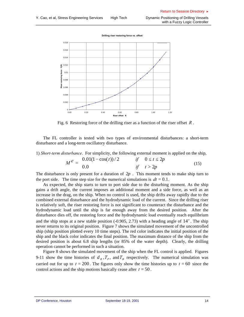
knots in x− direction. The water is about 1200 meters deep. The ship has a hull of Mariner class type. The hydrodynamic derivatives in Eq. (14) for this hull type can be found in Lewis (1989). The physical limitations imposed on the control devices are list in Table 5. The nondimensionalized restoring force of the riser (based on L , ρ and oU ) is shown in Fig. 6. In

the numerical simulations, when R is beyond the range in Fig. 6, the force )(RF is determined

by a linear extrapolation. GBL and rL are 0.4 and 0.2 respectively. The ship is initially located

at (0,0) with zero speed. The initial location is also chosen as the desired location. The objective of the FL control is to keep the ship as close as possible to this desired location with a desired heading angle of 0 degree.

Control device Maximum control value

Maximum rate of change

Rudder 300 20 per nondimensional unit time

Bow thruster 0.1 0.05 per nondimensional unit time

Propeller thrust increase 0.01 0.005 per nondimensional unit time

Table 5 Limitations on the control devices




Fig. 6 Restoring force of the drilling riser as a function of the riser offset R .

The FL controller is tested with two types of environmental disturbances: a short-term disturbance and a long-term oscillatory disturbance.

1) Short-term disturbance. For simplicity, the following external moment is applied on the ship,

>≤≤−

=π

π20.0

202/))cos(1(01.0

tif

tifteM (15)

The disturbance is only present for a duration of π2 . This moment tends to make ship turn to the port side. The time step size for the numerical simulations is 1.0=dt .

As expected, the ship starts to turn to port side due to the disturbing moment. As the ship gains a drift angle, the current imposes an additional moment and a side force, as well as an increase in the drag, on the ship. When no control is used, the ship drifts away rapidly due to the combined external disturbance and the hydrodynamic load of the current. Since the drilling riser is relatively soft, the riser restoring force is not significant to counteract the disturbance and the hydrodynamic load until the ship is far enough away from the desired position. After the disturbance dies off, the restoring force and the hydrodynamic load eventually reach equilibrium and the ship stops at a new stable position (-0.905, 2.73) with a heading angle of o14 . The ship never returns to its original position. Figure 7 shows the simulated movement of the uncontrolled ship (ship position plotted every 10 time steps). The red color indicates the initial position of the ship and the black color indicates the final position. The maximum distance of the ship from the desired position is about 6.8 ship lengths (or 85% of the water depth). Clearly, the drilling operation cannot be performed in such a situation.

Figure 8 shows the simulated movement of the ship when the FL control is applied. Figures 9-11 show the time histories of Rδ , PT , and BT respectively. The numerical simulation was

carried out for up to 200=t . The figures only show the time histories up to 60=t since the control actions and the ship motions basically cease after 50=t .

Drilling riser restoring force vs. offset

0

0.002

0.004

0.006

0.008

0.01

0.012

0.014

0.016

0.018

0.00 0.20 0.40 0.60 0.80 1.00 1.20

Riser offset R

Ris

er r

esto

rin

g f

orc

e F

(R)




X

Y

-8 -6 -4 -2 0 2-4

-3

-2

-1

0

1

2

3

4

5

6

Frame 001 15 Aug 2001 Ship PositionFrame 001 15 Aug 2001 Ship Position

Fig. 7 Ship trajectory due to the short-term disturbance (without control)

X

Y

-1 -0.5 0 0.5 1-1

-0.75

-0.5

-0.25

0

0.25

0.5

0.75

1


Fig. 8 Ship trajectory due to the short-term disturbance (with FL control)




Fig. 9 Time history of the rudder angle

Fig. 10 Time history of the increase in propeller thrust

Fig. 11 Time history of the bow thrust

- 2 . 0

- 1 . 0

0 . 0

1 . 0

2 . 0

3 . 0

4 . 0

5 . 0

6 . 0

7 . 0

8 . 0

0 . 0 1 0 . 0 2 0 . 0 3 0 . 0 4 0 . 0 5 0 . 0 6 0 . 0

t

Ru

dd

er a

ng

le (

deg

)

- 0 . 0 0 1 5

- 0 . 0 0 1 0

- 0 . 0 0 0 5

0 . 0 0 0 0

0 . 0 0 0 5

0 . 0 0 1 0

0 . 0 0 1 5

0 . 0 0 2 0

0 1 0 2 0 3 0 4 0 5 0 6 0

t

Pro

pel

ler

thru

st in

crea

se

- 0 . 0 1 0 0

- 0 . 0 0 5 0

0 . 0 0 0 0

0 . 0 0 5 0

0 . 0 1 0 0

0 . 0 1 5 0

0 . 0 2 0 0

0 . 0 2 5 0

0 . 0 3 0 0

0 1 0 2 0 3 0 4 0 5 0 6 0

t

Bo

w t

hru

st




As seen, the FL controller responds to the disturbance quite rapidly with a large rudder angle and bow thrust (see Fig. 9 and Fig. 11) to counteract the external moment. This prevents the ship

heading ψ and location ),( gg xx from growing (the ship would continue to move far away from

the original location if no control was applied, as shown in Fig. 7). Soon after the disturbance becomes weaker and eventually dies off, the FL controller is able to bring the ship to the original location with the desired heading. Clearly, the FL controller achieves the objective.

The maximum distance the ship is pushed away has been reduced to 0.06 ship length (or 0.75% of the water depth). After the disturbance dies off, the FL controller is able to keep the ship in its original position and the desired heading with error bounds of 0.25% of the ship length (or 0.03125% of the water depth) in position and o08.0± in heading. The performance of the FL controller is satisfactory. 2) Long-term random oscillatory disturbance. In this example, the drill ship is subject to a long-term random oscillatory disturbance,

0

)sin(

)sin(

)sin(

)(

1

)(

1

)(

1

≥

+=

+=

+=

∑

∑

∑

=

=

=

t

tMeM

tYeY

tXeX

Mjj

N

j

ej

Yjj

N

j

ej

Xjj

N

j

ej

e

e

e

βω

βω

βω

(16)

where e

jX , ejY and e

jM are the amplitudes of the force and moment components at frequency

jω . )( Xjβ , )(Y

jβ and )(Mjβ are the random phases uniformly distributed over )2,0( π . For the

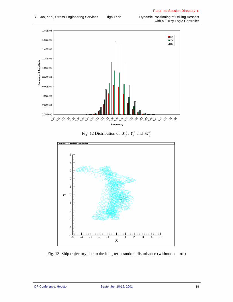
simulations shown here, 26 evenly spaced frequencies from 0.2 to 0.5 are used. The amplitudes of the forces and moment for the frequencies are shown in Figure 12. The red (or left), green (or middle) and white (or right) bars correspond to the forces in x and y directions and the yaw moment. The frequency corresponding to the peak amplitude is around 0.35. A time step size of

05.0=dt was used for this simulation. The duration of the simulation is 200. Figure 13 shows the trajectory of the ship with no control applied (plotted at every 15 time

steps). As seen, the ship is pushed as far as 5.2 ship lengths (or 65% of water depth) away from the desired location and the ship’s heading changes from o60− to o86 . Again, the drilling operation cannot be performed in this situation.

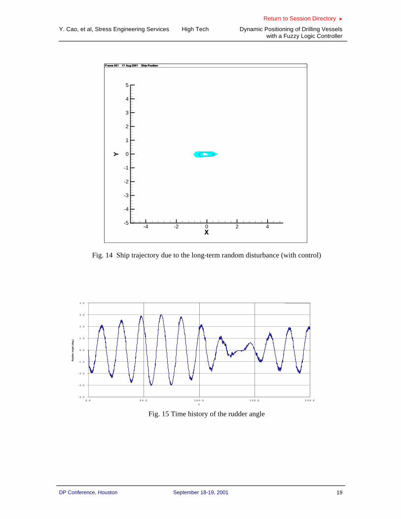
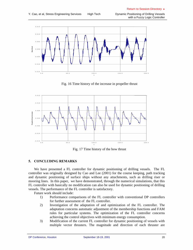
The trajectory of the ship with the FL control is shown in Fig. 14. Figures 15-17 show the time histories of Rδ , PT , and BT respectively. The FL controller responds to the environmental disturbance adequately and significantly reduces the movement of the ship. The maximum distance from the desired location has been reduced to 0.33 ship length (or about 4 % of the water depth) and the range of the heading to )32.1,22.1( oo− . The performance of the Fl controller is satisfactory.




Fig. 12 Distribution of ejX , e

jY and ejM

X

Y

-5 -4 -3 -2 -1 0 1 2 3 4 5-5

-4

-3

-2

-1

0

1

2

3

4

5


Fig. 13 Ship trajectory due to the long-term random disturbance (without control)

0.00E+00

2.00E-04

4.00E-04

6.00E-04

8.00E-04

1.00E-03

1.20E-03

1.40E-03

1.60E-03

1.80E-03

0.20

0.21

0.22

0.24

0.25

0.26

0.27

0.28

0.30

0.31

0.32

0.33

0.34

0.36

0.37

0.38

0.39

0.40

0.42

0.43

0.44

0.45

0.46

0.48

0.49

0.50

Frequency

Co

mp

on

ent

Am

plit

ud

eXe

Ye

Qe




X

Y

-4 -2 0 2 4-5

-4

-3

-2

-1

0

1

2

3

4

5


Fig. 14 Ship trajectory due to the long-term random disturbance (with control)

Fig. 15 Time history of the rudder angle

- 4 . 0

- 3 . 0

- 2 . 0

- 1 . 0

0 . 0

1 . 0

2 . 0

3 . 0

4 . 0

0 . 0 5 0 . 0 1 0 0 . 0 1 5 0 . 0 2 0 0 . 0

t

Ru

dd

er a

ng

le (

deg

.)




Fig. 16 Time history of the increase in propeller thrust

Fig. 17 Time history of the bow thrust

5. CONCLUDING REMARKS We have presented a FL controller for dynamic positioning of drilling vessels. The FL

controller was originally designed by Cao and Lee (2001) for the course keeping, path tracking and dynamic positioning of surface ships without any attachments, such as drilling riser or mooring lines. In this paper, we have demonstrated, through the numerical simulations, that this FL controller with basically no modification can also be used for dynamic positioning of drilling vessels. The performance of the FL controller is satisfactory.

Future work should include: 1) Performance comparisons of the FL controller with conventional DP controllers

for further assessment of the FL controller. 2) Investigation of the adaptation of and optimization of the FL controller. The

adaptation concerns automatic adjustment of the membership functions and FAM rules for particular systems. The optimization of the FL controller concerns achieving the control objectives with minimum energy consumption.

3) Modification of the current FL controller for dynamic positioning of vessels with multiple vector thrusters. The magnitude and direction of each thruster are

- 0 . 0 1 5

- 0 . 0 1 0

- 0 . 0 0 5

0 . 0 0 0

0 . 0 0 5

0 . 0 1 0

0 . 0 1 5

0 . 0 5 0 . 0 1 0 0 . 0 1 5 0 . 0 2 0 0 . 0

t

Pro

pel

ler

thru

st in

crea

se

- 0 . 0 1 5

- 0 . 0 1 0

- 0 . 0 0 5

0 . 0 0 0

0 . 0 0 5

0 . 0 1 0

0 . 0 1 5

0 . 0 5 0 . 0 1 0 0 . 0 1 5 0 . 0 2 0 0 . 0

t

Bo

w t

hru

st




variable and can be controlled by the FL controller for better dynamic positioning of the vessels.

6. ACKNOWLEDGEMENT

We would like to thank Dr. Robert Gordon of Stress Engineering Services, Inc. for providing the structural model of the drilling riser used in the simulations. The structural model was used to calculate the restoring force of the riser (Fig. 6). 7. REFERENCES

[1] CMPT (1998), “Floating Structures: a Guide for Design and Analysis”.

[2] Cao, Y. and Lee, T. (2001), “Maneuvering of surface vessels using a fuzzy logical controller”, submitted to Journal of ship Research.

[3] Cao, Y., Zhou, Z. and Vorus, W.S. (2000), “Application of a neural network predictor/controller to dynamic positioning of offshore structures”, Proceedings. Dynamic Positioning Conference (DP 2000), Society of Marine Technology, Houston, TX.

[4] DeBitetto, P.A. (1994), “Fuzzy logic for depth control of unmanned undersea vehicles”, Proceedings. Symposium on Autonomous Underwater Vehicle Technology, Cambridge, MA.

[5] Fang, M-C. and Chiou, S-C. (2000), “SWATH ship motion simulation based on a self-tuning fuzzy control”, Journal of Ship Research, Vol. 44, No. 2, pp. 108-119.

[6] Gu, M.X., Pao, Y.H. and Yip, P.P.C. (1993), “Neural-net computing for real-time control of a ship’s dynamic positioning at sea”, Computer Engineering Practice, 1 pp. 305-314.

[7] Ishii, K., Fujii, T. and Ura, T. (1994), “A quick adaptive method in a neural network based control system for AUVs ”, Proceedings, Symposium on Autonomous Underwater Vehicle Technology, Cambridge, MA

[8] Kosko, B. (1992), “Neural networks fuzzy systems – a dynamical systems approach to machine intelligence”, Prentice-Hall, Englewood, New Jersey.

[9] Lewis E. (1989), “Principles of naval architecture, Vol. III”, Society of Naval Architects and Marine Engineers.

[10] Li, D. and Gu, M.X. (1996), “Dynamic positioning of ships using a planned neural network controller”, Journal of Ship Research, Vol. 40, No.2

[11] Parsons, M.G., Chubb A.C. and Cao Y. (1995), “An assessment of fuzzy logic vessel path control”, IEEE Journal of Oceanic Engineering, Vol. 20, No. 4.

[12] Robert, G.N. (1997), “Approaches to fuzzy autopilot design optimization”, Proceedings, IFAC Conference on Maneuvering and Control of Marine Crafts, Brijuni, Croatia.

[13] Zhang, Y., Hearn, G.E. and Sen, P. (1997), “Neural network approaches to a class of ship control. Part I: Theoretical design, and Part II: Simulation studies”, Proceedings, 11th Ship Control Systems Symposium (Ed. Wilson, P.A.), University of Southampton, UK.

Documents

Committee - Dynamic positioningdynamic-positioning.com/proceedings/dp2001/high_tech_cao.pdf · Return to Session Directory > Y. Cao et al, Stress Engineering Services High Tech Dynamic