Embed Size (px)
Citation preview

FAA-RD-77-31
Project ReportATC-74
Coaxial Magnetron Spectra and Instabilities
M. Labitt
24 June 1977
Lincoln Laboratory MASSACHUSETTS INSTITUTE OF TECHNOLOGY
LEXINGTON, MASSACHUSETTS
Prepared for the Federal Aviation Administration, Washington, D.C. 20591
This document is available to the public through
the National Technical Information Service, Springfield, VA 22161

This document is disseminated under the sponsorship of the Department of Transportation in the interest of information exchange. The United States Government assumes no liability for its contents or use thereof.

Technical Report Documentation Page
1. Report No.
FAA-RD-77-3l
4. Title and Subtitle
2. Government Accession No. 3. Recipient's Catalog No.
5. Report Date
24 June 1977
1
,
Coaxial Magnetron Spectra and Instabilities
7 Author! s)
M. Labitt
9. Performing Organization Nome and Address
M.l. T. Lincoln LaboratoryP.O. Box 73Lexington, MA 02173
12. Sponsoring Agency Nome ond Address
Department of TransportationFederal Aviation AdministrationSystems Research and Development ServiceWashington, DC 20591
15. Supp lementory Notes
6. Performing Organization Code
8. Performing Orgoni zation Report No.
ATC-74
10. Work Unit No. (TI1AIS)
11. Contract or Grant No. Task KDOT-FA71-WAI-242
13. Type of Report and Period Covered
Project Report
14. Sponsori ng Agency Code
This work was performed at Lincoln Laboratory, a center for research operated by MassachusettsInstitute of Technology under Air Force Contract F19628-76-C-0002.
16. Abstract
Application of advanced radar clutter rejection techniques to FAA airport surveillanceand enroute radars is constrained by inherent instabilities and spectral properties of thedevice used in the radar transmitter to generate high level RF pulse energy, and the degreeto which its spectrum can be influenced by the circuit in which it operates. Coaxial magnetrons are believed to be spectrally pure, controllable and stable, and to embody othercharacteristics such as long life, which make them attractive replacements for the magnetrons presently employed. This report summarizes the results of extensive measurements made on a conventional S-band magnetron (presently employed in the ASR-7 radar)and a coaxial magnetron of equivalent pulse and power rating to compare their instabilitiesand spectral properties.
17. Key Wards
Coaxial MagnetronStabilitySpurious ResponseAirport Surveillance RadarsMOVing Target Indicator
18. Oi stri bution Statement
Document is available to the public throughthe National Technical Information Service,Springfield, VA 22151
19. Security Clonil. <01 this report)
Unclas sified
Form DOT F 1700.7 (8 - 7 Z)
20. Security Clossil. Col this poge)
Unclassified
Rcproduct ion of compl et ed page authori ccu
21. No. 01 Poges
74

APPENDIX - EFFECT OF PULSE-TO-PULSE FM ON THE PERFORMANCE OF ACOHERENT RADAR PROCESSOR SUCH AS THE LINCOLN LABORATORYMOVING TARGET DETECTOR (MTD)
I.
II.
III.
IV.
TABLE OF CONTENTS
INTRODUCTION
MAGNETRON OPERATION
A. Coaxial Magnetron
B. Conventional Magnetron
MEASUREMENT RESULTS
A. Short-Term Frequency Stability
1. Importance of Short-Term Frequency Stability
2. Measurement Technique
3. Coaxial Magnetron
4. Conventional Magnetron
B. Long-Term Frequency Stability
1. Coaxial Magnetron
2. Conventional Magnetron
C. Spurious Responses
1. Measurement Technique
2. Spectra of Magnetron Spurious Responses
D. Coaxial Magnetron Pulse Jitter
1. Measurement of Time Jitter
2. Effect of Pulse Shape Jitter
E. Pulling and Pushing Figures
F. Phase Locking the Coaxial Magnetron
G. OTP Compliance
CONCLUSIONS
iii
Page_l
2
2
2
7
7
7
9
14
14
14
16
16
16
16
19
51
51
51
57
57
59
59
62

1.
2.
3a.
3b.
4.
5.
6.
7.
8.
9a.
9b.
10.
11.
12.
ILLUSTRATIONS
RF pulse excessive fall-time caused by inductive control 3of rise time.
Diode network used to control magnetron voltage rate of rise. 4
V-I waveforms - coaxial magnetron (upper curve is I) (H-axis: 50.2 ~sec/div; V-axis: 10 amps/div and 5 kV/div).
I-P waveforms - coaxial magnetron (upper curve is linear P , 5notog~librated). 0
Typical coaxial magnetron spectrum (V-axis: 10 dB/div; H-axis: 62 MHz/div).
Coaxial magnetron spectrum using inductor in series with PFN 6(V-axis: 10 dB/div; H-axis: 2 MHz/div).
DX-276 spectrum using diode network and 10-section PFN (V-axis: 810 dB/div; H-axis: 10 MHz/div).
DX-276 spectrum using standard configuration (V-axis: 10 dB/div; 8H-axis: 10 MHz/div).
Short-term frequency stability test set-up. 10
Phase detector operation. 11
f of coaxial magnetron vs frequency. 15rms
Frequency drift and exhaust temperature rise of coaxial magnetron 17(QKH-1739LL); ASR-7 normal operating conditions.
Frequency drift and exhaust temperature rise of conventional magnetron 18(DX-276); ASR-7 normal operating conditions.
Two-way probe attenuation vs frequency. 20
13. through 29. Coaxial magnetron (QKH-1739LL) operating at 2.7 GHz.
iv
21-25

ILLUSTRATIONS (continued)
~
30. through 46.
Coaxial magnetron (QKH-1739LL) operated at 2.8 GHz.
47. through 63.
Coaxial magnetron (QKH-1739LL) operated at 2.9 GHz.
64. through 80.
Conventional magnetron (DX-276) operated at 2.7 GHz.
81. through 97.
Conventional magnetron (DX-276) operated at 2.8 GHz.
98. through 114.
Conventional magnetron (DX-276) operated at 2.9 GHz.
Page
26-30
31-35
36-40
41-45
46-50
115. RF envelope of coaxial magnetron as seen on a sampling scope. 52
116. Coaxial magnetron RF pulse injection. 52
117. Front edge of RF envelope 2 watts of priming.
118. Front edge of RF envelope - no priming.
119. Front edge of RF envelope - no priming
120. Phase error (rms) vs priming power.
l2l. OTP specification superimposed on co~.xial magnetron.
122. OTP specification superimposed on DX-276.
53
53
55
58
60
60
v

..
COAXIAL MAGNETRON SPECTRA AND INSTABILITIES
I. INTRODUCTION
This report covers measurements and analyses performed by Lincoln Laboratory
for the Federal Aviation Administration in order to compare the emissions of a
coaxial and a conventional magnetron operating in the frequency range of 2700 to
2900 MHz. The study was authorized under Task K of Interagency Agreement
DOT-FA7l-WAI-242 .
The coaxial magnetron investigated in this study was the Raytheon QK1739LL.
It was developed as a replacement tube for the magnetron presently used in the
ASR-7 airport surveillance radar. The conventional magnetron studied was the
*Amperex DX276 normally used in the ASR-7.
Magnetron characteristics measured and used as the basis of comparison
were:
short term stability (frequency jitter)
long term stability (thermal drift)
spurious response (18 GHz to waveguide cutoff)
pulse characteristics (applied voltage and current waveforms and timejitter)
pulling and pushing figures
compliance with OTP "Radar Spectrum Engineering Criteria", Part 5.
Sub tasks necessary to accomplish Task K were:
1. Develop, build and operate circuitry to
a. control the rate of rise of the voltage applied to the coaxial
magnetron.
b. inject a priming signal into the coaxial magnetron.
c. measure frequency jitter.
2. Determine the ability of the coaxial magnetron to lock to a low-level
priming signal.
*Equivalent to the Raytheon 5586 tube.

3. Ascertain the effect of the coaxial magnetron's priming signal on
rise-time jitter.
4. Seek techniques to improve the conventional magnetron spectrum by
the use of the special circuits developed to control the rate of rise of
applied voltage.
II. MAGNETRON OPERATION
A. Coaxial Magnetron
To perform the coaxial magnetron measurements an ASR-7 radar transmitter
and receiver were obtained. Modifications to the ASR-7 modulator were necessary
since the coaxial magnetron requires that the modulator generate a much slower
voltage pulse rise-time than the DX276 normally requires. If the rate of rise
is too fast (>65K volts per ~sec), the coaxial tube will tend to mode causing
the generation of off-frequency energy, severe modulator mismatch and RF rise
time jitter. A sudden threshold of moding does not appear to exist, however
the probability of moding rapidly increases with the rate of rise.
It was found that the present method of increasing rise time, i.e. adding
inductance in series with the pulse forming network (PFN), was inadequate. This
method did slow the rise time, but it also increased the fall time to such an
extent that the RF envelope was severely distorted (Figure 1), and the spectrum
degraded. Also, the additional inductance mismatched the modulator and essen
tially transformed the PFN into a one-section network.
In order to increase rise-time and not affect fall-time, a special non
linear diode network was developed. Its circuit is shown and its method of in
creasing rise-time without affecting fall-time is explained in Figure 2. A
typical spectrum using the diode network is shown in Figure 4. A coax magnetron
spectrum taken using the series inductance is shown in Figure 5.
B. Conventional Magnetron
Initially it was believed that the diode network concept would be useful in
controlling the spectrum of the DX276. In the normal configuration a two-section
PFN is used together with an RC despiking network. This results in a long RF
2

WI
l ATC-74(1) L
Fig. 1. RF pulse excessive fall-time caused by inductive controlof rise time.
3

l ATC-74(2) 1__Operation of Diode Network of Fig. 2: After the first pulse, the 250 pf
capacitor charges to the magnetron pulse voltage and then decays to a valuebelow the conduction voltage of the magnetron. This voltage is set by theZener diode stack. On the second and subsequent pulses, the fast recoverydiodes are normally biased off. When the magnetron pulse is applied thecapacitor loads the pulse transformer increasing the rise time after thepulse voltage exceeds the Zener stack voltage. This loading only lastsapproximately as long as the time constant RC = 250 nsec, where R = 1000ohms is the source impedance of the modulator. •
The result is that the magnetron voltage rises rapidly at first,(as shown by the more distinct trace in Fig. 3a), then abruptly slows downjust before the magnetron starts to conduct and oscillate. (The RF envelopeis shown as the more distinct trace in Fig. 3b). Notice that when themodulator pulse shuts off, the charge on the capacitor does not dischargethrough the magnetron to produce a long RF pulse tail, but instead dischargesharmlessly through the Zener stack.
diode stack
Magnetron
Diode network
FastRecoveryDiodeStackOutput
PulseTransformer
Fig. 2. Diode network used to control magnetron voltage rate of rise.
4
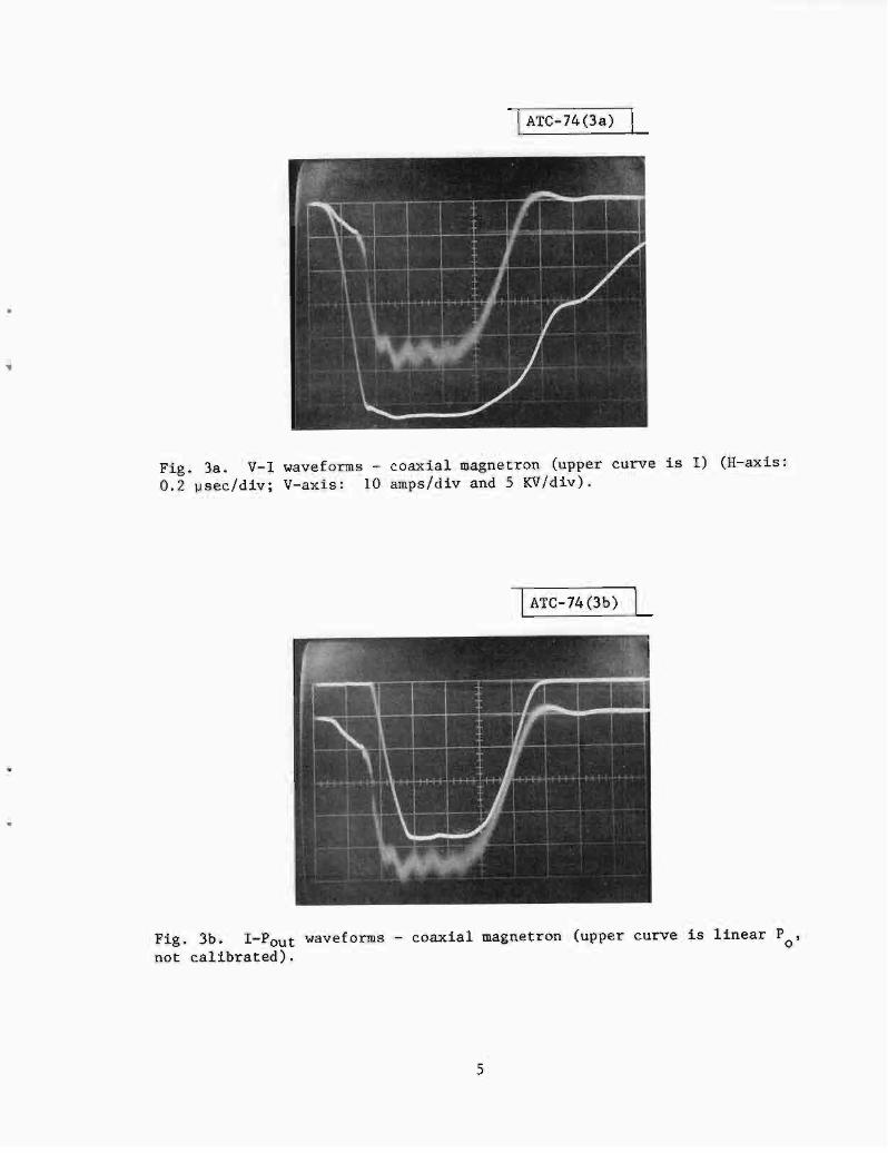
l ATC-74(3a) l-
Fig. 3a. V-I waveforms - coaxial magnetron (upper curve is I) (H-axis:0.2 ~sec/div; V-axis: 10 amps/div and 5 KV/div).
l ATC-74(3b) ~
Fig. 3b. I-Pout waveforms - coaxial magnetron (upper curve is linear P ,not calibrated). 0
5

l ATC-74(4) L
Fig. 4. Typical coaxial magnetron ~pectrum (V-axis: 10 dB/div; H-axis:2 MHz/div).
l ATC-74(5) L
Fig. 5.(V-axis:
Coaxial magnetron spectrum using inductor in series with PFN10 dB/div; H-axis: 2 MHz/div).
6

tail which causes the high side lobes on the low frequency side of the spectrum.
To control the long tail the old PFN was replaced with a lO-section network.
This network reduced the fall-time but also reduced the rise-time. The diode
network was then used to control the fast rise time (as with the coax magnetron)
in order to prevent the tube from moding.
Figure 6 shows the spectrum using the lO-section network and the diode
network. Figure 7 shows the standard configuration spectrum. An improvement
is apparent but it is not deemed worth the additional complexity. DX276 measure
ments described in the rest of this report are all made using the standard con
figuration of the ASR-7 radar transmitter/modulator.
III. MEASUREMENT RESULTS
A. Short-Term Frequency Stability
1. Importance of Short-term Frequency Stability
Modern MTI radar processors require that the transmitter have a high
degree of frequency stability. The effect of frequency fluctuation can be demon
strated by the following situation. Consider the radar return from two ranges
separated by a half a pulse length at the same azimuth. Upon arrival at the
radar the two returns will partially overlap. If the radar frequency varies from
pulse to pulse, then the resultant signal level at the overlap point will fluctuate.
Most modern MTI devices process the signal after the steady component has been
removed. Thus, in a conventional MTI radat frequency instability will increaseI
the number of false alarms, while in a CFAR MTI the frequency instability will
result in a loss of sensitivity.
Consider a perfectly stable radar (other than the magnetron frequency) look
ing at stationary clutter and define the ratio of the fluctuation to steady com
ponents as ¢, T the pulse length; then the relationship to the frequency filter
is:
frms
13¢TIT
*(1)
------------*Equations (1) and (2) are derived in the Appendix.
7

-I ATC-74(6) I~
Fig. 6. DX-276 spectrum using diode network and 10-section PFN (V-axis:10 dB/div; H-axis: 10 MHz/div).
-I ATC-74(7) L
..
Fig. 7.H-axis:
DX-276 spectrum using standard configuration (V-axis:10 MHz/div.
8
10 dB/div;

if the coho is locked to the center of the magnetron pulse. If the coho is
locked to the tail of the pulse, then the requirement is more stringent,
frms
__13¢2nT
*(2)
Normally the coho is locked to the tail, but it does not prove to be much of
a problem to do mid-pulse locking. If a residue-to-c1utter ratio of 0.16 x 10⁻⁴
(-48 dB) and a pulse length of 0.7 ~sec are assumed, then for a center-locking
system, the magnetron jitter should not exceed
f rms 3150 Hz (3)
A ¢ of -48 dB represents a loss in the processor improvement factor of 0.64 dB
when operating at a clutter-to-thermal-noise ratio of 40 dB.
2. Measurement Technique
A short-term frequency stability measurement setup is shown in Figure 8.
An attenuated sample of the RF pulse is mixed down to 30 MHz and then split into
two paths; one delayed and the other not. The delay consists of a length of
cable and is 0.35 ~sec long corresponding to about half the magnetron pulse
length. The effect is to beat the first half of the pulse with the back half.
The response of a phase detector is
E kAB sin e
where E is the output voltage, A and B are the amplitudes of the two signals,
k is a constant and e the phase difference. Notice that E can only be greater
than zero when both A and B are greater than zero. Consequently, the phase
detector output will appear on a scope as in Figure 9a in an idealized form.
A sample and hold (S/H) is set to sample the phase detector in the center of the
overlap. The line stretcher is adjusted so that 8 is near zero and, as a result,
the output of the sample and hold is proportional to the phase difference, e,as long as e is small.
9

Sample from!-!agnetron r-------,
2800
30 MHz
Line Stretcher
Cable Delay
l ATC-74(8) L
DC volt meter ~v
S/H A/D 3 Pulsecanceller D/A
RMS
oVoltmeter
Trigger Clockingtrigger
Fig. 8. Short term frequency stability test set-up.
10

TA!C-74(9a)L
Undelayed envelope 1 Delayed pulse envelope
~~ I-~-I- -_£-;-. - - -: -I - : : •
1 A I 1 liBI
Phase I 'KAB sin Q1___.Sampling Time
Fig. 9a. Phase d~tector operation.
11

The relationship between the magnetron jitte~ f ,and e can be determinedrmsby tracing the signal through the various components (Figure 8). The FM jitter
at RF is converted down to the same amount of jitter at the 30-MHz IF. The phase
at the phase detector is therefore,
e 21T fIF
T
where fIF
is the FM'd IF frequency;and T is the cable delay time. A change in eis given by
or
erms21T T f
rms
where f is the standard deviation of the magnetron frequency and defined asrms
frms
rE {(f - E {f })2t/2~ mag mag 1
where E{ } is the expectation (averaging) operator. Notice that f is not reallyrms
the rms value of the frequency, but the rms value of the difference from the mean.
However, this definition is common and will be used here.
In order to measure e it is necessary to first remove the DC component.rms
This is accomplished by converting the signal out of the "sample and hold" (S/H) to
digical and then through a 3-pulse canceller (as in an MTI system). The signal
is then converted back to analog and finally fed to an rms voltmeter. In addition
to removing the DC component, the 3-pulse canceller removes the effect of any slow
drift of phase (or frequency). Such drift would not affect an MTI system.
The 3-pulse canceller has the following response,
R E - 2 E 1 + E 2n n n- n-
where E is the nth voltage sample. Thus, the rms voltmeter measures thisn
quantity,
12

Because E and E are not correlated.n m
E {E E}n m
E En m
-2E
where the bar denotes the average. Thus,
R [E {En2
- 2 E En-l + E En-2rms n n
-2 E En
_l
+ 4 E2
- 2 En-l En-2n n-l
E2 }]1/2
+ E En-2 - 2 E E +n n-l n-2 n-2
[6 {E2}-2 ] 1/2
E - 6 En
or
Rrms
16 Erms
Calibration is necessary and is performed in the following manner. The
line stretcher, on the LO, is first adjusted so the DC voltmeter (Figure 8) in
dicates zero. Then the line stretcher is moved a known distance, 6£, and the
corresponding change in DC voltage 6vnoted. The phase shift per volt is
then,2n 6£ f rF-------
C 6V
where AIF is the IF wavelength and C is the velocity of light. Remembering
thate
f rmsrms 2n T
and Re rms lie
rms 16 6V
we can condense all of the above to
13

f rms
3. Coaxial Magnetron
It was determined that heater power, and to a lesser extent operating
frequency, affects the short-term frequency stability of the coaxial magnetron.
All other parameters appear to have a minor effect. Figure 9b shows the stan
dard deviation of frequency (f ) as a function of both heater voltage andrms
output frequency. The nominal heater voltage for any magnetron depends on the
particular value of average anode power applied and, for this situation, is
about 58 volts. The standby voltage is 70 volts. It can be seen that stability
markedly improves as the heater voltage is raised to presumably an excessive
value. Both Raytheon and Lincoln believe that this phenomenum is peculiar and
does not represent the capability of the coaxial magnetron. Raytheon believes
it to be a cathode phenomenum (perhaps caused by the leakage of cathode material
over the end caps) and that the effect can be eliminated by a different cathode
design. Such different cathode designs have been used in the production of
higher frequency coaxial magnetrons. As it stands now, the only way to have
this magnetron meet the requirements of Eq. (3) is to raise the heater voltage
to 70 volts. Raytheon believes this will not shorten tube life.
4. Conventional Magnetron
Measurements of the Amperex DX276 have been made at 2.7, 2.8 and 2.9
GHz. No statistically significant differences were noted. Unlike the coaxial
tube, the DX276 is not heater power sensitive. The standard deviation of fre
quency was measured several times at each frequency and found to be
+f = 2068 - 660 Hz
B. Long-Term Frequency Stability
Measurements have been taken on both magnetrons of the shift in frequency
and the rise in temperature that occurs when the tubes are first turned on.
Such information is useful in determining how much frequency bandwidth is
occupied during warmup.
14

l ATC-74(9b)L
f"ltd-, 'titt!· ,-1-+
8 oj. -;.-~ I
12 ~l~ r\! J . +jt'1 :tt-8Jlmmlfft-HFrmmmBIEE1t±lUBfEfEmmma-+ . ++++h-H~'+ r'vP-l'+'l'¥'I-P+f'+'lflh mag 11 ~rb
U,n-.HllmrmmfUftlf!E1-'11TfL~ if-i'tt_tff-lE,n- r-t-"
tt:~::tt:tt:tt:tt~ttl:tJ~ztqJtztliTr-rTE,B=t+E'rn~=El-J-tij:- tEEEEtai=El1nnaftEE=E=EElE10 1-+-I-+-l--H+++++++i'IlH--+--f-JH-i--H++++++H--1-+-H-i--H++++++++1-+-H-I--H+++++++-r-H--H-1-H-++++++++H--H
+
Fig. 9b. f of coaxial magnetron vs frequency.rrns
15

The frequency drift was measured by observing the spectrum drift across the
screen of a spectrum analyzer. Because the anode portion of the tube was in
accessible, the temperature of the coaxial tube was measured by recording the
temperature of air coolant exhausting from the tube. The temperature of the
5586 was measured using thermo-couples directly attached to the tube anode.
1. Coaxial Magnetron
The frequency temperature shift of the QK1739 is plotted in Figure 10
for three trials. The maximum frequency drift is about 1.5 MHz and takes about
an hour to occur. No frequency change occurred until about 3-4 minutes had
elapsed even though the exhaust temperature has started to rise. The exhaust
temperature levels out to about 48°C.
2. Conventional Magnetron
Figure 11 illustrates how the DX276 drifts during warmup. Note that
half of the total frequency excursion of 7 MHz occurs in 8 minutes. In contrast,
the coaxial tube takes about 18 minutes to drift to half its total excursion.
The frequency drift rate is greatest at turnon. The anode temperature reads
900 C, half of which occurs in the first four minutes.
C. Spurious Responses
1. Measurement Technique
Spectral measurements using the Hewlett-Packard l41T spectrum analyzer
(8555A RF section, 8552B IF section and 8445B tracking preselector) have been
made of the two magnetrons operating at 2.7, 2.8 and 2.9 GHz. The
dynamic range (linear) of the H-P analyzer is limited to about 60 dB. Con
sequently, in order to extend the range to the required 100 dB, a notch filter
was employed to suppress most of the main lobe energy. This allowed the signal
strength (sensitivity) outside the main lobe area to be increased so that
any spurious responses 100 dB down from the main lobe would be observable. At
frequencies above the main lobe the notch filter passband is not flat and
therefore is ineffective. Here C, X and K-band waveguides were used to remove
the main lobe. The signal from the probe went through a coax to waveguide
16

--:
1--.
15
00
, ,.
J,.
.cl'
••
~f
;-"
+,'
+t::
:r "i-+
r-t:.
j-t
.+~
++,
I
t
lAT
C-7
4(1
0)
I'I·
-20
-10
010
20[)
40
50
60
7080
Rela
tiv
eT
ime
(min
ute
s)
Fig
.1
0.
Fre
qu
ency
drif
ta
nd
ex
ha
ust
tem
pera
ture
ris
eo
fco
ax
ial
ma
gn
etr
on
(QK
H-1
739L
L);
AS
R-7
no
rma
lo
pera
tin
gco
nd
itio
ns.

a'J-"
81
~FrequencyDrift(MHz)
S""iIIIr"'
OQOQ;::l0
(0rt....~.... o0
;::l
........""it:I~:><(1)1..0N~-....1(1)O\::l'-/nwo0...:::
~p..tn~
:;dr"'lH'l
-....Irt
;::lIIIo::l~p..III(1)f-lX
::r oIII'1j~
(0iCIl~rtIIIrtrtr"-ro::lS
OQ'1j(0
(j~
oIII;::lrtp..~
r"-~
rtror"-o~;::lr"'rnrnoro
oH'l
('l
o~ro::lrtr"'o;::lIIIf-l
r~r.it.•.m'~..·.-.r.Ij-f-i-IT'Tffi.X'.tT+:T0'.;f UiJ...•.,t!J~l"-"i,"~TF:.'..t"'".'.'.1
§~+~.l'++..jt-..i.1',', 'II.'•t-...l_',~!tt,.,,-
1+IFT·,t"at:::~ot+t"iljl-r:.:HI:f'"
..,,,t;.c
l'iImt'i ''·1·..t"+.-H..'...I.:',.'"';' +It't-.~".
Etr
';'Irr'iit1'111J.lj.+,,.i--i"T'
+.'1;1~_~lS+ijJ!.+t+U,:L~1=ci~~:_.i':_:~tt-t
+hIt.j<,.r!i.ttf+.tItl.w.l...-tHI':=;i+T,'.+-ijrtH1,,1;[~trl'"+
'f...;~'1\'[._,1"::Lii-,j'!"~....'i",~-H-~'it\.+-+f-H~Jl+-,,':-;,~:
t1t:':.:.'..-+-:(r1l:
"HI!'!!,"~WiIIIItfl'~niH ttJ:H..+.'.ffi'H.11,",.H'....'...'.tit',it'jt-';','I T..,,~-ljTH!..j1+"1
:!Ii11"'\",II".'!III':;-j~wtff'--iiJ{.iiHji.Jlt-ql,+._.~.11--_t~-if~tH'i-flTnIi'"0;-+-t;it·L'i'tj--H'
~'Hj-.fll±t[It1r1,!ll).i'i·:'r,:t'rtf: 1t+.=;.f-ttll...11.1Ttt'"c':l;jj>-J1.TI'.c.t.'".:~'1f-:.'r:fI ~'11jt....1-.'·'i~.__:t-','ro-";If!+-t.',,-j.jT',f-,·,~0:T++'11Ii.",-j..1.::-'
:J:f-l\#tH_l,;'t' :;IIIITH~-,I,II
~IIII,I'li1.i"I!1+ ~it!.8.\+.1st1Ii.tj'.;;..J
~Ll'.,tttl--,'j,Ltmm''-+--1.f'4,,,~' ILm1,-'jr1rj;,;.':11+j
i_~1f=£-,IIj-fdIftrttfll:l;:.::1-
1
,1,
d-J+H,t:r't1='':,Irnjt+.t'I!i-IL
gtiJijj~!IJItIirnr,IlI;!inl -H'~IItTI+f''.jIIt-1tI, ITii't...1.''..~IL11fI~t·..f!JCill-l'-'r-..I·1t
!"e11'1..,+lilt-' ~j~+1.•.-_:-'-Itt.
Ii'j._I·tII.fi-hI.,:'I1'.~if[1-f-.t.'.-tHt-I:!l!tt~
~I-H:iL1.--j=r.,tIt=-tt~tIf~I,I.:i' I.~t~!I,,'I,
,r:tr-t-r--+-i'HH·lr+j.."-=fIi','"
a~JLill1tJih~~rt~-,nITf1.-l-l..I.+.Jl.i~t''r.1;.;'.;',
t}I.f-f-+-ittrttt!£fI~-t1
It"_:,)',tI-ttt-t~tJJ~rht:-;d:rl,rt.J+.!.d.ITiH::.:.,lli: ::1',:,~iIIPjLt+ItTIt',LIri-~:+11'1!:.t'I.i.
T
f~ r+,j,Ii;:i"I:Iij;::~;,:11:,ilt:
I~
l~J

transistion, then through a 3-ft section of WRl12, WR187 or WR90 waveguide,
then back to coax and, thence to the spectrum analyzer.
Measurement of spurious responses from waveguide cutoff to 18 GHz re
quires that the pick-off, probe, directional coupler or whatever attenuates
the signal to the analyzer, have a flat frequency response over this region.
No such device is available. Complicating the problem is the existence of
high order modes in the S-band waveguide at the upper frequencies. In order
to simplify the problem, a small capacitive probe was used to sample the electric
field in the waveguide. Ignoring higher order modes, such a probe would be
expected to have an attenuation inversely proportional to frequency. The probe
was calibrated by inserting two identical probes in the waveguide and measur-
ing the attenuation between the two as a function of frequency. A scattering
of values was obtained as shown in Figure 12. The attenuation of one probe
is then assumed to be half (in dB) the attenuation of both. A best fit straight
line approximation shows the one-way attenuation to go as (f)-1.28, which is
approximately inversely proportional to frequency. An approximate probe cor
rection formula can be inferred from Figure 12, i.e.
+c = 25.6 10glO f - 11.5 - 5
where c is the additional sensitivity (in dB) one has as a function of frequency
f (in GHz). Thus, at 18 GHz the spectra are 20.6 dB more sensitive, making
the 60 dB below the main lobe level really 80.6 dB below the main lobe.
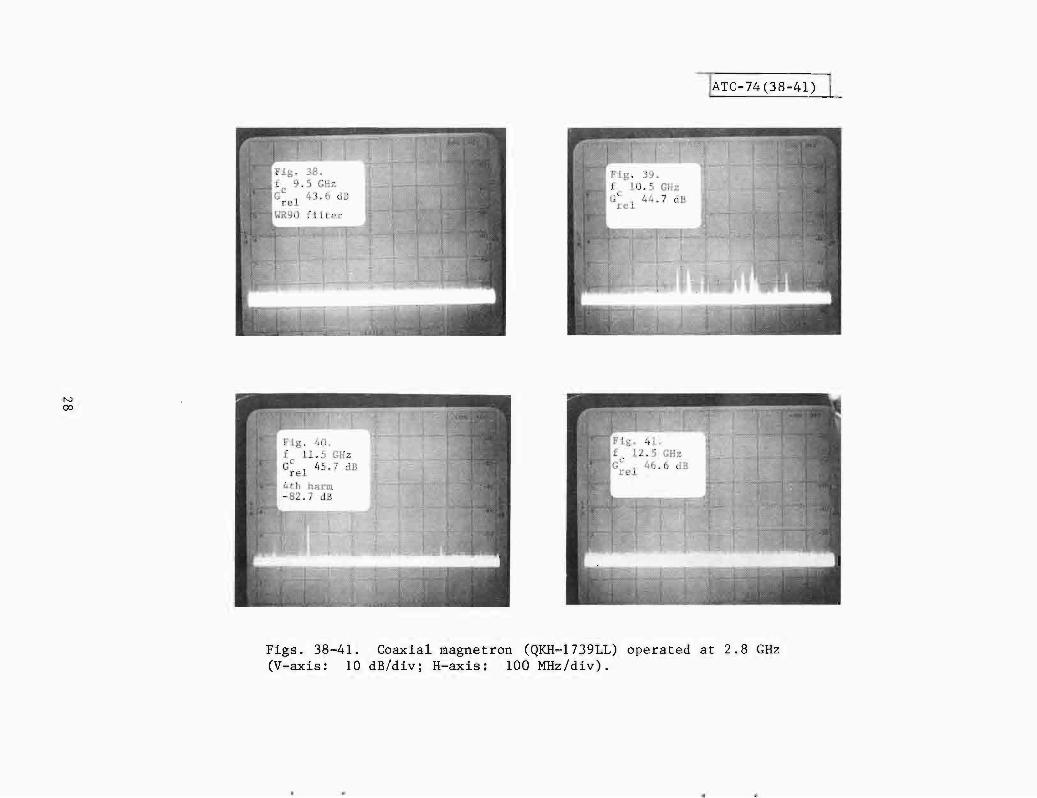
2. Spectra of Magnetron Spurious Responses
The table given below indexes sets of figures showing photographs of the
spurious responses obtained on each magnetron at low, mid and upper test fre
quencies. The caption block on the face of each spectrum photograph identifies
the frequency at the center of the analyzer screen (fJ, the relative gain setting
(G 1) and the level of harmonic energy if present. Conditions under which eachre
spurious response spectrum was photographed are identical to those for the pre-
viously numbered spectrum figure except for the conditions noted in the individual
figure captions.
19

AT
C-7
4(12
)F
req
uen
cy-
GH
z
N o-5
0I
,
+rt
i
:.1'
,
'1T
".T~
"
",
:-:-
~
1'1
W--
..0
.~,;+
,++j-
7080
~o~oo
60
"':
j
30
20
, i=i=
---+
+
108
96
54
", ,
I,
~Lu4"':::::'
-'-'-t'+~
,'-.
:
.L':
':..
.._
.
.
'c.
~r-
,"cw
··..~
....
•.
ci'!
'.~j_.
,~.~
_.
.
.l+-
17''
'';,
~iT
t~.".
=-.~
F:'-
III
I---
:--t-
II
!il
--
==~
-70
-60
f(G
Hz)
Fig
.1
2.
Two~way
pro
be
att
en
ua
tio
nV
Bfr
equ
ency
.

",
-~TC-74(13-16)
L
N .....
Fig
.1
5.
F3
.5G
Hz
c G1
32
.5dB
reW
R18
7F
ilte
r
No
no
tch
Fig
.1
6.
f4
.5G
Hz
cG
13
5.3
dBre
Fig
s.13~16.
Co
ax
ial
mag
net
ron
(QK
H-1
739L
L)
op
era
ted
at
2.7
GH
z(V
-ax
is:
10d
B/d
iv;
H-a
xis
:1
00
MH
z/d
iv).

~ATC-74(17-20)
l-
N N
Fig
s.1
7-2
0.
Co
axia
lm
agn
etro
n(~KH~1739LL)
op
era
ted
at
2.7
GH
z(V
-ax
is:
10d
B/d
iv;
H-a
xis
:10
0M
Hz/
div
).
•

.,
lAT
C-7
4(2
1-2
4)L
N Vol
Fig
s.2
1-2
4.
Co
axia
lm
agn
etro
n(Q
KH
-173
9LL
)o
pera
ted
at
2.7
GH
z(V
-ax
is:
10d
B/d
iv;
H-a
xis
:10
0M
Hz/
div
).

lAT
C-7
4(2
5-2
8)
\_
Figs~
25-2
8.C
oax
ial
mag
netr
on
(QK
H-1
739L
L)
op
era
ted
at
2.7
GH
z(V
-ax
is:
10
dB
/div
;H
-ax
is:
10
0M
Hz/
div
).

to
Fig. 29.(V-axis:
-I ATC-74(29) L
Coaxial magnetron (QKH-1739LL) operated at 2.7 GHz10 dB/div; H-axis: 100 MHz/div).
25

~TC-
74(3
0-33
)
Fig
s.30~33.
Co
axia
lm
agn
etro
n(Q
KH
-173
9LL
)o
per
ated
at
2.8
GH
z(V
-ax
is:
10d
B/d
iv;
H-a
xis
:10
0M
Hz/
div
).

lATC
-74
(34
-37
)1_
Fig
s.34~37.
Co
axia
lm
agn
etro
n(~KH~1739
LL
)oper~ted
at
2.8
GH
z(V
-ax
is:
10d
B/d
iv;
H-a
xis
:10
0M
Hz/
div
).
]AT
C-7
4(38
-41)
L
N 00
Fig
s.3
8-4
1.
Co
axia
lm
agn
etro
n(QKH~1739LL)
op
erat
edat
2.8
GH
z(V
-ax
is:
10d
B/d
iv;
H-a
xis
;10
0M
Hz/
div
).

lAT
C-7
4(4
2-4
5)
L
Fig
s.42~45.
Co
axia
lm
agn
etro
n(QKH~1739LL)
op
erat
edat
2.8
GH
z(V
-ax
is:
10d
B/d
iv;
H-a
xis
:10
0M
Hz/
div
).

Fig. 46.(V-axis:
l ATC-74(46) L
Coaxial magnetron (QKH-1739LL) operated at 2.8 GHz10 dB/div; H-axis: 100 MHz/div).
30

•
lAT
C-7
4(4
7-5
0)
L
Fig
s.4
7-5
0.
Co
axia
lm
agn
etro
n(Q
KH
-173
9LL
)o
pera
ted
at
2.9
GH
z(V~axis:
10d
B/d
iv;H~axis;
100
MH
z/d
iv).
-~TC-74(5l-54)
L
W N
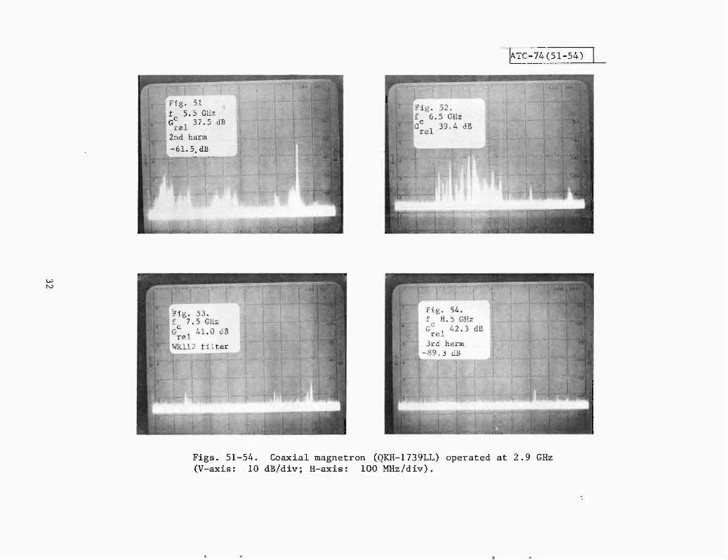
Fig
s.5
1-5
4.
Co
axia
lm
agn
etro
n(Q
KH
-173
9LL
)o
per
ated
at
2.9
GH
z(V
-ax
is:
10d
B/d
iv;
H-a
xis
:10
0M
Hz/
div
).

lAT
C-7
4(5
5-5
8)
L
Fig
s.55~58.
Co
axia
lm
agn
etro
n(Q
KH
-173
9LL
)o
per
ated
at
2.9
GH
z(V
-ax
is:
10d
B/d
iv;
H-a
xis
:10
0M
Hz/
div
).

--!A
TC
-74(
59-6
2)l-
Fig
s.5
9-6
2.
Co
axia
lm
agn
etro
n(Q
KH
-173
9LL
)o
per
ated
at
2.9
GH
z(V
-ax
is:
10d
B/d
iv;
H-a
xis
:10
0M
Hz/
div
).

-I ATC-74(63) L
Fig. 63.(V-axis:
Coaxial magnetron (QKH-1739LL) operated at 2.9 GHz10 dB/div; H-axis: 100 MHz/div).
35

--~T
C-74
(64-
67)~
Figs~
64~67.
Co
nv
en
tio
nal
mag
net
ron
(DX~276)
op
era
ted
at
2.7
GH
z(V~axis:
10d
B/d
iv;
H~axis:
10
0M
Hz/
div
).
•

.'
-~TC-74(68-71)
LF
ig.
68.
f5
.5G
Hz
GC
13
7.5
dBre 2n
dh
arm
-57
.5dB
Fig
s.6
8-7
1.
Co
nv
enti
on
alm
agn
etro
n(D
X-2
76)
op
erat
edat
2.7
GH
z(V
-ax
is:
10d
B/d
iv;
H-a
xis
;10
0M
Hz/
div
).

Fig
.7
3.
f1
0.5
GH
zc
Gre
14
4.7
dB
i-IR
90fil
ter;
4th
har
m-7
0.7
dB
w 00
~TC-74(72-75)
Fig
s.72
...75
.C
on
ven
tio
na
lm
ag
net
ron
(DX
-276
)o
pera
ted
at
2.7
GH
z(V
-ax
is:
10d
B/d
iv;
H-a
xis
:1
00
MH
z/d
iv).

~ATC
-74(
76-7
9)l-
Fig
s.7
6-7
9.
Co
nv
enti
on
alm
agn
etro
n(D
X-2
76)
op
erat
edat
2.7
GH
z(V
-ax
is:
10d
B/d
iv;
H-a
xis
:10
0M
Hz/
div
).

Fig. 80.(V-axis:
l ATC-74(80) L
Conventional magnetron (DX-276) operated at 2.7 GHz10 dB/div; H-axis: 100 MHz/div).
40

• ~TC-74(81-84)
Fig
s.81~S4.
Co
nv
enti
on
alm
agn
etro
n(D
X-2
76)
op
erat
edat
2.8
GHz
(Y-a
xis
:10
dB
/div
;H
-ax
is:
100
MH
z/d
iv).

Fig
.8
8.
f8
.5G
Hz
cG
14
2.3
dBre 3rd
har
m-6
8.3
dB
-\A
TC
-74
(85
-88
)1_
Fig
s,85
.--88
,C
onve
nti
onal
mag
net-
ron
(PX
..,..2
76)
op
era
ted
at
2.8
GH
z(V~is:
10d
B/d
iv;
H-a
xis
:10
0M
Hz/
div
).

• -~TC-74((89-92)L
Fig
s.8
9-9
2.
Co
nv
enti
on
alm
agn
etro
n(D
X-2
76)
op
erat
edat
2.8
GH
z(V
-ax
is:
10d
B/d
iv;
H-a
xis
:10
0M
Hz/
div
),

-IA
TC
-74
(93
-96
)l-
Fig
s.93~96.
Co
nv
en
tio
nalmagnetr~n
(DX
-276
)o
pera
ted
at
2.8
GH
z(V~axis:
10d
B/d
iv;
H-a
xis
:1
00
MH
z/d
iv).

Fig. 97.(V-axis:
-I ATC-74(97) L
Conventional magnetron (DX-276) operated at 2.8 GHz10 dB/div; H-axis: 100 MHz/div).
45

~TC-
74(9
8-10
1)1_
Fig
s.98~101.
Co
nv
enti
on
alm
agn
etro
n(D
X-2
76)
op
era
ted
at
2.9
GH
z(V
-ax
is:
10d
B/d
iv;
H-a
xis
:10
0M
Hz/
div
).
•

--~T
C-74
(102
-l05
~
Fig
s.1
02
-10
5.
Co
nv
enti
on
alm
agn
etro
n(D
X-2
76)
op
erat
edat
2.9
GH
z(V
-ax
is:
10d
B/d
iv;
H-a
xis
:10
0M
Hz/
div
).

~TC-74(106-109)L
Fig
s.1
06
-10
9.
Co
nv
enti
on
alm
agn
etro
n(D
X-2
76)
op
erat
edat
2.9
GH
z(V
-ax
is:
10d
B/d
iv;
H-a
xis
:10
0M
Hz/
div
).
t'
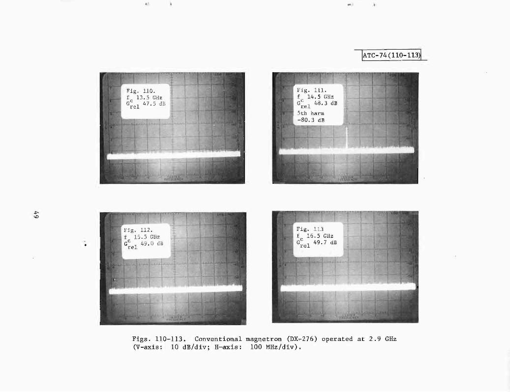
lAT
C-7
4(1
10
-11
3)L
•
Fig
s.1
10
-11
3,
Co
nv
enti
on
alm
agn
etro
n(D
X-2
76)
op
erat
edat
2.9
GH
z(V
-ax
is:
10d
B/d
iv;
H-a
xis
:10
0M
Hz/
div
).

Fig. 114.(V-axis:
-I ATC-74(114) L
Conventional magnetron (DX-276) operated at 2.9 GHz10 dB/div; H-axis: 100 MHz/div).
50
•

Figures NumberedMagnetron 2.7 GHz 2.8 GHz 2.9 GHz
Coaxial (QKH-1739LL) 13 thru 29 30 thru 46 47 thru 63
Conventional (DX276) 64 thru 80 81 thru 97 98 thru 114
D. Coaxial Magnetron Pulse Jitter
1. Measurement of Time Jitter
Conventional magnetrons have a small amount of time jitter compared
to coaxial magnetrons. The amount of jitter is generally so small as to have
little effect in most radar applications. Because the jitter is small and
because of the difficulty of measuring such small time differences, only measure
ments of the coaxial magnetron were made.
Figure 115 shows the RF envelope of the QK1739LL coaxial magnetron as viewed
on a sampling oscilloscope under the following conditions.
(1) The standard diode network controlling the rate of rise was used
(as described in Section II).
(2) A 2-watt RF pulsed signal was injected into the magnetron during
the turn-on time of the modulator pulse to the magnetron. The RF circuit
is shown in Figure 116.
In Figure 117 the front edge of the RF envelope is expanded to show the
starting jitter with the priming signal. The scope is triggered from the front
edge of the applied modulator voltage pulse. The jitter is estimated to have a
standard deviation of 3 nsecs. Without pJiming (Figure 118), the jitter deviation
increases to about 10 nsecs.
2. Effect of Pulse Shape Jitter
The effect of pulse shape jitter on the performance of an MTI radar
is now discussed. A magnetron transmitter pulse that has pulse shape jitter may
be analyzed by treating it as the sum of two pulses, a steady and a fluctuating
pulse. The fluctuating component is uncorrelated (the magnetron has no memory)
and will affect the MTI processor as white noise. The ratio of the steady com
ponent power to the noise power represents the maximum c1utter-to-noise ratio
that can be tolerated without reducing the radar sensitivity. It is necessary
to calculate the noise-to-clutter ratio ~ given an arbitrary jitter across the
pulse.
51

IATC-74(115) L
Fig. 115. RF envelope of coaxial magnetron asseen on a sampling scope (V-axis: linear power not calibrated; H-axis: 0.2 ~sec/div; pulse is0.7 ~sec long at half-power points).
l ATC-74(116~ L
Circulator Load
Trigger
2 IJatt- ....-.; s-Band
ulse Gen
Fig. 116. Coaxial magnetron RF pulse injection.
52
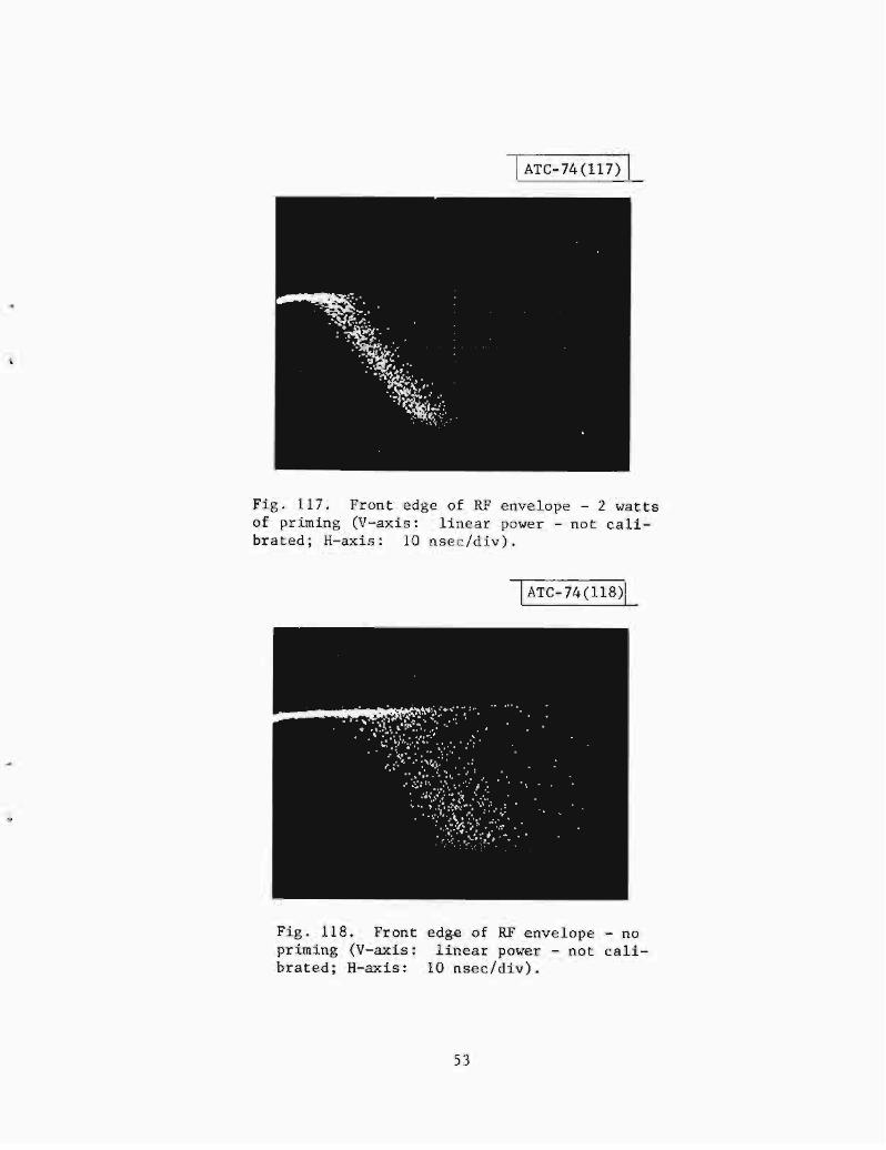
-I ATG-74(117) I
fig. 117. Front edge of RF envelope - 2 wattsof priming (V-axis: linear power - not calibrated; H-axis: 10 nsec/div).
Fig. 118. Front edge of RF envelope - nopriming (V-axis: linear power - not calibrated; H-axis: 10 nsec/div).
53

Let V (t) represent the magnetron amplitude waveform of the nth pulse. V (t)n n
is a random variable. V(t) is defined as the mean of V (t). The normalizedn
clutter return from a point target is just
while the residual noise caused by the jitter is
(4)
where the integrals are taken over the pulse and E{ } is the expectation opera
tor. Thus, the noise-to-c1utter ratio is
fo 2(t) dtv .
f V2(t) dt
(5)
where
2 -2Since V (t) ~ V (t), the denomina-
The numerator is more in-
of the pulse (Figure 119) and2o (t) cannot be estimated
vpictures are of the output of
o 2 is by definition the variance of V.v
tor is simply the peak power times the pulse length.
vo1ved. 0 2(t) is greatest at the beginningv
tapers to zero at t = 125 nsec. Unfortunately,o
directly from Figure 119. This is because these
a square-law detector and represent power.
Looking at Figure 117 and 119, one can represent the time jitter (standard
deviation) as 1i~ear1y decreasing
o (t) = 0 (1-t ot
tt
o) o < t < t
o(6)
t < to
where 0 is the initial time jitter and t is the time when the jitter vanishes.ot 0
If one lets the normalized power be represented by
- -2p = V
then lip 2 V II V1/2
2 p II V
and
54

Fig. 119. Front edge of RF envelope - nopriming (V-axis: linear power - not calibrated; H-axis: 50 nsec/div) .
••
55

a (t)p
1/22 P a (t)
v
1/2a «p
v(7)
From Figure 119 one sees that
p = m t
where m is the rise time slope. Thus,
a (t) = m a (t)p t
Combining (6), (7) and (8)
o < t < to
o < t < to
(8)
(9)
2 m 2 (1 - t )2 o < t <a4t
a tv ot t 0
0
Consequently, Eq. (5) becomes t0
2 J _ -.!.) 2 dtm a(1ot a -
4t t t
<P0 0 (10)
Pmax L
where L is the pulse length at the half power points. The integration cannot
be taken from zero because of the pole at t 0 and the requirement that
a «pl/ 2 '(Eq. (7). From Figure 117 and 118 one can estimate thatv
and
aot
aot
sec with priming
without priming
Thus,
L
m
-77 x 10 sec
P /2.1 x 10-7 watts/secmax
<Ptiming jitter
<Ptiming jitter
-44 dB (priming)
-36 dB (no priming)
This value can be compared to the value of <P caused by the coaxial magnetron
frequency jitter. The value of <P obtained when the heater is optimally adjusted
is
56

<P freq • jitter -52 dB (f - 2 kc)rms
,
It would, therefore, appear that timing jitter is more of a problem than
frequency jitter and that priming is necessary.
E. Pulling and Pushing Figures
The pushing figure experiment consists of applying square wave modulation
to the high voltage pulse to the magnetron. The resultant peak-to-peak fre
quency current deviation constitutes the pushing figure. The frequency shifts
were observed both on a spectrum analyzer and on a phase detector as in the
frequency jitter tester. The current shifts were monitored on a scope by the
use of a current transformer in the anode line to the magnetron. The pushing
figures measured were:
Coaxial magnetron:
DX276:
4.5 kHz/ampere
31. 0 kHz / ampere
Pulling figure is defined as the peak-to-peak frequency shift of the mag
netron when the magnetron is subjected to 1.5 VSWR at all phase angles. The
mismatch was generated by inserting a teflon slab into a longitudinal slot in
the waveguide. By sliding the slab longitudinally in the slot all phases are
generated. The pulling figures measured were:
Coaxial magnetron:
DX276:
1.23 GHz at 2.80 GHz
7.4 MHz at 2.86 GHz
F. Phase Locking the Coaxial Magnetron
Because priming the coaxial magnetron greatly reduces the timing jitter, it
was thought that the priming signal could be used to phase lock the magnetron.
In essence the magnetron would become an "amplifier" and one would have a co
herent transmitter. Measurements of the rms phase error of the magnetron rela
tive to the priming signal were made at four different priming powers (up to
6 kW). A plot of the rms phase error e (standard deviation) is shown inrms
Figure 120. At 6 kW the e is 2.7 degrees. This corresponds torms
erms 2
10 log ( 360 X 2n)
57
-26.5 dB

oo~
(sacl.Illap)suu
6
58
,
000~
I-lQ)
~00-
ClOt::
Ul .~
'"' .~'"''" I-l~0-
CIl::-,...
CIl0 e,0~ 'oJ
I-l0I-lI-lQ)
<1lCIlIII
..c::p.,
0N..-l
0 ClO~
.~
f%.<
..

It appears that it would require an excessive amount of priming (in the
order of the magnetron output power itself) in order to develop a reasonable
~ of -40 dB.
G. OTP Compliance
The Office of Telecommunications Policy (OTP) radar design objectives are
inappropriate in the context of the present study. The OTP design objectives*
relate the allowed spectral bandwidth to the rise time of the RF envelope; the
longer the rise time the narrower the bandwidth. There is little one can do to
control the rise time of a magnetron, coaxial or standard. Because coaxial
tubes have a longer rise time, the OTP objectives require that the coaxial
tube operate in narrower bandwidth. Figures 121 and 122 illustrate this point.
Figure 121 is the coaxial magnetron spectrum with the OTP specs overlaid, while
Figure 122 is the standard tube. Notice that the standard tube is allowed twice
the bandwidth of the coaxial tube. In spite of this restriction, the coaxial
tube is within OTP specs while the DX276 is not.
IV. CONCLUSIONS
Measurements have been made of a coaxial magnetron, the Raytheon QK1739LL,
and a conventional magnetron, the Amperex DX276, in order to compare their per
formance. Each has advantages over the other. Whether one is better overall
than the other depends on the situation. Some of the disadvantages can be cor
rected by the radar design. The following is a list of comparative magnetron
properties, and following it is an assessment of whether they are significant.
The plus (+) indicates superiority.
PullingPushingFrequency JitterTime JitterSpurious SpectrumLong-term StabilityLifetimeBreak-in TimeCost
Coaxial
++
++++
Standard
++
+
*OTP Manual of Regulations and Procedures for Radio Frequency Management, Chapter 5,Section 5.3 (January 1973).
59

lATC-74(l21)L
Fig. 121. OTP specification superimposed oncoaxial magnetron (V-axis: 10 dB/div; H-axis:5 MHz/div).
Fig. 122. OTP specification superimposed onDX-276 (V-axis: 10 dB/div; H-axis: 10 MHz/div).
60

Pulling; can be alleviated by the use of an isolator or circulator. The
ASR-7 uses a circulator; therefore, it is not a problem for either tube.
Pushing: can be reduced by good modulator design. The ASR-7 is probably
adequate for either tube.
Frequency Jitter: is intrinsic and is not affected by modulator design.
Time Jitter; is intrinsic and the most serious problem of coaxial tubes.
It can be partially corrected by priming and rise time control. The ASR's already
have a circulator that can be used to inject the priming signal.
The Near-in Spurious Spectrum of either tube cannot be improved, however
harmonics and high frequencies could be removed with waveguide filters.
Long-Term Stability can be corrected by AFC-ing the magnetron with respect
to a crystal-controlled local oscillator. The crystal oscillator has the
stability needed for a high performance MTI or MTD system.
The Lifetime and reliability of coaxial magnetrons is expected to be much
greater than that of the standard magnetron because of its larger internal
structure. This structure permits lower electric fields, essentially eliminat
ing sparking and Break-in Time.
The coaxial tube Costs about a factor of 10 more than the standard tube.
The cost may be reduced by mass production and/or a competitive market.
61

APPENDIX
EFFECT OF PULSE-TO-PULSE FM ON THE PERFORMANCE OF A COHERENT
RADAR PROCESSOR SUCH AS THE LINCOLN LABORATORY MOVING TARGET DETECTOR (MTD)
INTRODUCTION
The frequency instability of a magnetron in a radar manifests itself as a
modulation of the return from an interval of clutter. This modulation can be
either periodic or random. The periodic modulation is caused, for example, by
external perturbations of the magnetron via the high voltage power supply, the
heater supply or external AC magnetic fields. These effects can be removed by
careful modulator and power supply designs. However, there is an intrinsic
random modulation that exists in all magnetrons and different magnetrons have
differing stabilities. It is the effect of this random noise modulation on the
radar performance that is treated here.
THEORY
Consider an extent of radar clutter return,C(t). For our purposes the
clutter return is frozen and the antenna is not rotating. The clutter does not
vary from one pulse interperiod to the next. That is:
(1)1
(prf) )C (t -C(t)
where: (prf) is the pulse repetition frequency. C(t) is considered to be fine
structured compared to the magnetron pulse length and of the order of a half
wave length of the radar frequency. Thus, C(t) has a resolution of about 5 cm
for an S-band radar. If we let the magnetron RF pulse envelope be represented by
u(t) and the phase deviation of the magnetron from its norm by 8(t), then the
return from a stationary point reflector becomes
u(t)~
i8(t):= e
.,.,. ,.01
The squiggle above 8(t) is to remind one that 8(t) is a random variable (rv). The
signal returning to the radar is then
62

-.S/(t) = c'<t)@ u(t) eie(t) (2)
'''1where ~ represents the convolution operator. C(t) fluctuates only during an-interpulse period, while Set) can fluctuate between periods. The average value
1\0''''of Set) at the time t is then
",--"Set) = C(t) ~ u(t) (3)
~'I
Notice that Set) is still a random variable but only during the interpulse
period. Most radar processors (MTD, MTI cancellers) remove Set), consequently~~ 1'\
".,.. -the residue Set) - Set) is of prime importance. The variance of Set) is the
average power remaining after the mean has been removed. The variance is given
by
(4)
where E{ } is the expectation operator (or average) and the asterisk represents
the complex conjugate. Thus, the quantity
2cr
-~ {~2}
is the residue-to-clutter ratio and is a measure of the magnetron stability.
Applying (2) and (3) we have
Because 8(t) is of the order of a few degrees, the following approximation is
made.
cr2
= E {['e'(t) ® u(t) i8 (t) ] [2*(t) ® u(t) (-i) 8(t)] } (6)
The magnetron envelope is assumed to extend from T to T + T and to have ao 0
rectangular shape. Thus, from the definition of convolution we have
63

or
T +T T +T0 0
2 f ~~ ~ f """* .M
a = E C(t- T) e(t) dt C (t" - T) 8(t") dt" (7)
T T0 0
E
T
JO
+T
~,11 "",,* ,w\
C(t" - T) C (t - T) 8(t)T
o
8(t") dt dt" (8)
....'" ~*" ~ 4'\A"Since C(t - T) C (t -T) and 8(t) 8(t ) are independent random variables, we
can apply the expectation operator separately,
2a
where
TfO+T
R (t - t" ) E te(t) 8'( t ") }T c
o
dt dt" (9)
{ ~ 4"*" }R (t - t") = E C(t - T) C (t - T)c
is approximately an impulse shaped covariance function. Thus, we can evaluate
the inner integral and find
(10)
where: C is the area under the impulse function R • That is0 c
00
C ~ f R (t) dt0 c
_00
64

.-The function G(t) is not known. however it cannot be a constant otherwise no
FM could take place. The simplest time dependence would be of the linear form
...-<1
G(t);vIA
= wt (11)
2o
Any higher order dependence cannot be measured with our present equipment and it
is not clear that it exists. L0 is a random variable representing the random
frequency error of the magnetron. Taking (11) as our model we find
T +T
fo
t2
dtT
o
In a similar manner we find
E{~2}c
o3
(12)
T +T
JT
o
R (t-t~) dt dt~c
C To
(13)
Thus the residue-to-clutter ratio is:
(T + T)3 - TE l~2} 0 3T 0 (14)
The lowest residue occurs when To
T/2. then:
(15)
This corresponds to locking the coho to the center of the magnetron pulse. If
the coho is locked to the tail-end of the magnetron pulse. T = -T. then:o
(16)
65

EXAMPLE OF THE RAYTHEON QK1739 COAXIAL MAGNETRON IN THE ASR-7
If we assume a residue-to-c1utter ratio ¢ of 0.16 x 10⁻⁴
and a pulse length
of 0.7 microseconds, then for a center-locking system
f rms1~
2TIT
12TI
3150 Hz
In the magnetron stability te$ter the output is given by
where Td
is the delay line delay of 0.35 microseconds and ~ is the gain of the
three-pulse canceller to a white random signal. Thus, the output (in degrees) is:
e < 360 f T ~rms rms d 0.97 degrees
If tail-end locking is used, then 0.49 degrees is required. The value of-4¢ = 0.16 x 10 was chosen to limit the loss in processor improvement factor to
0.64 dB when operating at a c1utter-to-therma1 noise ratio (C/N) of 40 dB.
10 log (N/C + .16 N/C) = 0.64 dBN/c
If we were to allow the residue ¢ to be equal to the thermal noise N, the im
provement ratio'wou1d deteriorate by 3 dB. ¢ would be equal to 10-4 and the
output of the stability tester would be
erms2TIT
(18)
This happens to be equal to the value measured for the coaxial magnetron at
2700 MHz at its nominal heater power. At higher heater power (which may reduce
tube life) e can drop to 0.5 degrees.rms
66

CONCLUSION
A model has been proposed to calculate the effect of pulse-to-pulse FM
of magnetrons in the presence of clutter on the performance of a coherent
processor. It establishes a simple relation between frequency stability and
clutter rejection useful in predicting the performance of magnetron radars.
67

ACKNOWLEDGEMENT
Acknowledgement is given to Mr. Harry P. McCabe, Engineering Assistant.
Mr. McCabe set up the equipment, performed virtually all the measurements and
provided many useful suggestions.
68