Numerical Comparison of CVaR and CDaR Approaches:Application to Hedge Funds1

Pavlo Krokhmal, Stanislav Uryasev, and Grigory Zrazhevsky

Risk Management and Financial Engineering LabDepartment of Industrial and Systems Engineering

University of Florida, Gainesville, FL 32611

This paper applies risk management methodologies to optimization of a portfolio

of hedge funds (fund of funds). We compare two recently developed risk manage-

ment methodologies: Conditional Value-at-Risk and Conditional Drawdown-at-Risk.

The common property of the risk management techniques is that they admit the

formulation of a portfolio optimization model as a linear programming (LP) prob-

lem. LP formulations allow for implementing efficient and robust portfolio allocation

algorithms, which can successfully handle optimization problems with thousands of

instruments and scenarios. The performance of various risk constraints is investigated

and discussed for in-sample and out-of-sample testing of the algorithm. The numerical

experiments show that imposing risk constraints may improve the “real” performance

of a portfolio rebalancing strategy in out-of-sample runs. It is beneficial to combine

several types of risk constraints that control different sources of risk.

1 Introduction

This paper applies risk management methodologies to the optimization of a port-folio of hedge funds (fund of funds). We compare risk management techniquesbased on two recently developed risk measures, Conditional Value-at-Risk andConditional Drawdown-at-Risk (Rockafellar and Uryasev 2000, 2002, Chekhlovet al. 2000). Both risk management techniques utilize stochastic programmingapproaches and allow for construction of linear portfolio rebalancing strategies,and, as a result, have proven their high efficiency in various portfolio manage-ment applications (Andersson et al. 2001, Chekhlov et al. 2000, Krokhmal et al.2002, Rockafellar and Uryasev 2000, 2002). The choice of hedge funds, as a sub-ject for the portfolio optimization strategy, was stimulated by a strong interestto this class of assets by both practitioners and scholars, as well as by challengesrelated to relatively small datasets available for hedge funds.

Recent studies2 of the hedge funds industry are mostly concentrated onthe classification of hedge funds and the relevant investigation of their activity.However, this paper is focused on possible realization of investment opportuni-ties existing in this market from the viewpoint of portfolio rebalancing strategies(for an extensive discussion of stochastic programming approaches to hedge fundmanagement, see Ziemba 2002).

1This work was partially supported by the Foundation for Managed Derivatives Research.2See, for example, papers by Ackermann et al. 1999, Amin and Kat 2001, Brown and

Goetzmann 2000, Fung and Hsieh 1997, 2000, 2001, and Lhabitant 2001.

1

Hedge funds are investment pools employing sophisticated trading and ar-bitrage techniques including leverage and short selling, wide usage of derivativesecurities etc. Generally, hedge funds restrict share ownership to high net worthindividuals and institutions, and are not allowed to offer their securities to thegeneral public. Many hedge funds are limited to 99 investors. This private na-ture of hedge funds has resulted in few regulations and disclosure requirements,compared for example, with mutual funds (however, stricter regulations exist forhedge funds trading futures). Also, the hedge funds may take advantage of spe-cialized, risk-seeking investment and trading strategies, which other investmentvehicles are not allowed to use.

The first official3 hedge fund was established in the United States byA. W. Jones in 1949, and its activity was characterized by the use of shortselling and leverage, which were separately considered risky trading techniques,but in combination could limit market risk. The term “hedge fund” attributesto the structure of Jones fund’s portfolio, which was split between long posi-tions in stocks that would gain in value if market went up, and short positions instocks that would protect against market drop. Also, Jones has introduced an-other two initiatives, which became a common practice in hedge fund industry,and with more or less variations survived to this day: he made the manager’sincentive fee a function of fund’s profits, and kept his own capital in the fund,in this way making the incentives of fund’s clients and of his own coherent.

Nowadays, hedge funds become a rapidly growing part of the financial in-dustry. According to Van Hedge Fund Advisors, the number of hedge fundsat the end of 1998 was 5830, they managed 311 billion USD in capital, withbetween $800 billion and $1 trillion in total assets. Nearly 80% of hedge fundshave market capitalization less than 100 million, and around 50% are smallerthan $25 million, which indicates high number of new entries. More than 90%of hedge funds are located in the U.S.

Hedge funds are subject to far fewer regulations than other pooled invest-ment vehicles, especially to regulations designed to protect investors. This ap-plies to such regulations as regulations on liquidity, requirements that fund’sshares must be redeemable an any time, protecting conflicts of interests, assur-ing fairness of pricing of fund shares, disclosure requirements, limiting usage ofleverage, short selling etc. This is a consequence of the fact that hedge funds’ in-vestors qualify as sophisticated high-income individuals and institutions, whichcan stand for themselves. Hedge funds offer their securities as private place-ments, on individual basis, rather than through public advertisement, whichallows them to avoid disclosing publicly their financial performance or assetpositions. However, hedge funds must provide to investors some informationabout their activity, and of course, they are subject to statutes governing fraudand other criminal activities.

As market’s subjects, hedge funds do subordinate to regulations protectingthe market integrity that detect attempts of manipulating or dominating in

3Ziemba (2002) traces early unofficial hedge funds, such as Keynes Chest Fund etc., thatexisted in the 1920’s to 1940’s.

2

markets by individual participants. For example, in the United States hedgefunds and other investors active on currency futures markets, must regularlyreport large positions in certain currencies. Also, many option exchanges havedeveloped Large Option Position Reporting System to track changes in largepositions and identify outsized short uncovered positions.

In this paper, we consider problem of managing fund of funds, i.e., con-structing optimal portfolios from sets of hedge funds, subject to various riskconstraints, which control different types of risks. However, the practical use ofthe strategies is limited by restrictive assumptions4 imposed in this case study:1) liquidity considerations are not taken into account, 2) no transaction costs,3) considered funds may be closed for new investors, 4) credit and other riskswhich directly are not reflected in the historical return data are not taken intoaccount, and 5) survivorship bias is not considered. The obtained results can-not be treated as direct recommendations for investing in hedge funds market,but rather as a description of the risk management methodologies and portfoliooptimization techniques in a realistic environment. For an overview of the po-tential problems related to the data analysis and portfolio optimization of hedgefunds, see Lo (2001).

Section 2 presents an overview of linear portfolio optimization algorithmsand the related risk measures, which were explored in this paper. Section 3contains description of our case study, results of in-sample and out-of-sampleexperiments and their detailed discussion. Section 4 presents the concludingremarks.

2 Risk management using Conditional Value-at-

Risk and Conditional Drawdown-at-Risk

Formal portfolio management methodologies assume some measure of risk thatimpacts allocation of instruments in the portfolio. The classical Markowitz the-ory, for example, identifies risk with the volatility (standard deviation) of aportfolio. In this study we investigate a portfolio optimization problem withthree different constraints on risk: Conditional Value-at-Risk (Rockafellar andUryasev 2000, 2002), Conditional Drawdown-at-Risk (Chekhlov et al. 2000),and the market-neutrality (“beta” of the portfolio equals zero)5. CVaR andCDaR risk measures represent relatively new developments in the risk manage-ment field. Application of these risk measures to portfolio allocation problemsrelies on the scenario representation of uncertainties and stochastic program-ming approaches.

A linear portfolio rebalancing algorithm is a trading (investment) strategywith mathematical model that can be formulated as a linear programming (LP)problem. The focus on LP techniques in application to portfolio rebalancing and

4These assumptions can be relaxed and incorporated in the model as linear constraints.Here we focus on comparison of risk constraints and have not included other constraints.

5There are different interpretations for the term “market-neutral” (see, for instance,BARRA RogersCasey 2002). In this paper market neutrality means zero beta.

3

trading problems is explained by the exceptional effectiveness and robustness ofLP algorithms, which becomes especially important in finance applications. Re-cent developments (see, for example, Andersson et al. 2001, Carino and Ziemba1998, Carino et al. 1998, Chekhlov et al. 2000, Consigli and Dempster 1997,1998, Dembo and King 1992, Duarte 1999, Krokhmal et al. 2002, Rockafellarand Uryasev 2000, 2002, Turner et al. 1994, Zenios 1999, Ziemba and Mul-vey 1998, Young 1998) show that LP-based algorithms can successfully handleportfolio allocation problems with thousands and even millions of decision vari-ables and scenarios, which makes those algorithms attractive to institutionalinvestors.

In the cited papers, along with Conditional Value-at-Risk and ConditionalDrawdown-at-Risk, other, much earlier established measures of risk, such asMaximum Loss, Mean-Absolute Deviation, Low Partial Moment with power oneand Expected Regret6, have been employed in the framework of linear portfoliorebalancing algorithms (see, for example, Ziemba and Vickson 1975). Some ofthese risk measures are quite closely related to CVaR concept7. We restrictedourselves to considering CVaR- and CDaR-based risk management techniques.

However, the class of linear trading or portfolio optimization techniques is farfrom encompassing the entire universe of portfolio management techniques. Forexample, the famous portfolio optimization model by Markowitz (1952, 1991),which utilizes the mean-variance approach, belongs to the class of quadraticprogramming (QP) problems; the well-known constant-proportion rule leads tononconvex multiextremum problems, etc.

2.1 Conditional Value-at-Risk

The Conditional Value-at-Risk (CVaR) measure (see Rockafellar and Uryasev2000, 2002) develops and enhances the ideas of risk management, which havebeen put in the framework of Value-at-Risk (VaR) (see, for example, Duffieand Pan 1997, Jorion 1997, Pritzker 1997, Staumbaugh 1996). Incorporatingsuch merits as easy-to-understand concept, simple and convenient representa-tion of risks (one number), applicability to a wide range of instruments, VaRhas evolved into a current industry standard for estimating risks of financiallosses. Basically, VaR answers the question “what is the maximum loss, whichis expected to be exceeded, say, only in 5% of the cases within the given timehorizon?” For example, if daily VaR for the portfolio of some fund XYZ is equal

6Low partial moment with power one is defined as the expectation of losses exceedingsome fixed threshold, see Harlow (1991). Expected regret (see, for example, Dembo and King1992) is a concept similar to the lower partial moment. However, the expected regret may becalculated with respect to a random benchmark, while the low partial moment is calculatedwith respect to a fixed threshold.

7Maximum Loss is a limiting case of CVaR risk measure (see below). Also, Testuri andUryasev (2000) showed that the CVaR constraint and the low partial moment constraintwith power one are equivalent in the sense that the efficient frontier for portfolio with CVaRconstraint can be generated by the low partial moment approach. Therefore, the risk manage-ment with CVaR and with low partial moment leads to similar results. However, the CVaRapproach allows for direct controlling of percentiles, while the low partial moment penalizeslosses exceeding some fixed thresholds.

4

to 10 millions USD at the confidence level 0.95, it means that there is only a5% chance of losses exceeding 10 millions during a trading day.

The formal definition of VaR is as follows. Consider a loss function f(x,y),where x is a decision vector (e.g., portfolio positions), and y is a stochasticvector standing for market uncertainties (in this paper, y is the vector of returnsof instruments in the portfolio). Let Ψ(x, ζ) be the cumulative distributionfunction of f(x,y),

Ψ(x, ζ) = P [f(x,y) ≤ ζ].

Then, the Value-at-Risk function ζα(x) with the confidence level α is the α-quantile of f(x,y) (see Figure 1):

ζα(x) = minζ∈R

{Ψ(x, ζ) ≥ α} .

Using VaR as a risk measure in portfolio optimization is, however, a very dif-ficult problem, if the return distributions of a portfolio’s instruments are notnormal or log-normal. The optimization difficulties with VaR are caused by itsnon-convex and non-subadditive nature (Artzner et al. 1997, 1999, Mausser andRosen 1998). Non-convexity of VaR means that as a function of portfolio posi-tions, it has multiple local extrema, which precludes using efficient optimizationtechniques.

The difficulties with controlling and optimizing VaR in non-normal portfolioshave forced the search for similar percentile risk measures, which would alsoquantify downside risks and at the same time could be efficiently controlled andoptimized. From this viewpoint, CVaR is a perfect candidate for conducting a“VaR”-style portfolio management.

For continuous distributions, CVaR is defined as an average (expectation)of high losses residing in the α-tail of the loss distribution, or, equivalently, as aconditional expectation of losses exceeding the α-VaR level (Fig. 1). From thisfollows that CVaR incorporates information on VaR and on the losses exceedingVaR.

For general (non-continuous) distributions, Rockafellar and Uryasev (2002)defined α-CVaR function φα(x) as the α-tail expectation of a random variablez,

φα(x) = Eα−tail [z],

where the α-tail cumulative distribution functions of z has the form

Ψα(x, ζ) = P [z ≤ ζ] ={

0, ζ < ζα(x),[Ψ(x, ζ) − α

]/[1 − α

], ζ ≥ ζα(x).

Also, Acerbi et al. (2001), Acerbi and Tasche (2001) redefined expected shortfallsimilar to the CVaR definition presented above.

Along with α - CVaR function φα(x), the following functions called “upper”and “lower” CVaR (α-CVaR+ and α-CVaR−), are considered:

φ+α (x) = E [f(x,y)|f(x,y) > ζα(x)],

5

Portfolio loss

Fr

eq

ue

nc

yVaR

CVaR

Probability

Maximum

loss

Figure 1: Loss distribution, VaR, CVaR, and Maximum Loss.

φ−α (x) = E [f(x,y)|f(x,y) ≥ ζα(x)].

The CVaR functions satisfy the following inequality:

φ−α (x) ≤ φα(x) ≤ φ+

α (x).

Rockafellar and Uryasev (2002) showed that α-CVaR can be presented as aconvex combination of α-VaR and α-CVaR+,

φα(x) = λα(x) ζα(x) + [1 − λα(x)] φ+α (x),

whereλα(x) = [Ψ(x, ζα(x)) − α]/[1 − α], 0 ≤ λα(x) ≤ 1.

For a discrete loss distribution, where the stochastic parameter y may takevalues y1,y2, ...,yJ with probabilities θj , j = 1, ..., J , the α-VaR and α-CVaRfunctions respectively are8

ζα(x) = f(x, yjα),

φα(x) =1

1 − α

jα∑

j=1

θj − α

f(x,yjα) +

J∑j=jα+1

θjf(x,yj)

,

where jα satisfiesjα−1∑j=1

θj < α ≤jα∑

j=1

θj .

For values of confidence level α close to 1, Conditional Value-at-Risk coincideswith the Maximum Loss (see Figure 1).

8This proposition has been derived in assumption that, without loss of the generality,scenarios y1,y2, ...,yJ satisfy inequalities f(x, y1) ≤ ... ≤ f(x, yJ ).

6

While inheriting some of the nice properties of VaR, such as measuringdownside risks and representing them by a single number, applicability to in-struments with non-normal distributions etc., CVaR has substantial advantagesover VaR from the risk management standpoint. First of all, CVaR is a convexfunction9 of portfolio positions. Hence, it has a convex set of minimum pointson a convex set, which greatly simplifies control and optimization of CVaR.Calculation of CVaR, as well as its optimization, can be performed by meansof a convex programming shortcut (Rockafellar and Uryasev 2000, 2002), wherethe optimal value of CVaR is calculated simultaneously with the correspond-ing VaR; for linear or piecewise-linear loss functions these procedures can bereduced to linear programming problems. Also, unlike α-VaR, α-CVaR is con-tinuous with respect to confidence level α. A comprehensive description of theCVaR risk measure and CVaR-related optimization methodologies can be foundin Rockafellar and Uryasev (2000, 2002). Also, Rockafellar and Uryasev (2000)showed that for normal loss distributions, the CVaR methodology is equivalentto the standard Mean-Variance approach. Similar result also was independentlyproved for elliptic distributions by Embrechts et al. (2002).

0

0.001

0.002

0.003

0.004

0.005

0.006

0.007

1 3 5 7 9 11 13 15 17 19 21 23 25 27 29 31 33 35

time (business days)

Portfolio value DrawDown function

Figure 2: Portfolio value and drawdown.

According to Rockafellar and Uryasev (2000, 2002), the optimization prob-lem with multiple CVaR constraints

minx∈X

g(x)

subject to φαi (x) ≤ ωi, i = 1, ..., I,

is equivalent to the following problem:

minx∈X, ζk∈R, ∀k

g(x)

9For a background on convex functions and sets see Rockafellar (1970).

7

subject to ζk +1

1 − αk

J∑j=1

θj max {0, f(x,yj) − ζk} ≤ ωk, k = 1, ..., K,

provided that the objective function g(x) and the loss function f(x,y) are con-vex in x ∈ X . When the objective and loss functions are linear in x and con-straints x ∈ X are given by linear inequalities, the last optimization problemcan be reduced to LP, see Rockafellar and Uryasev (2000, 2002).

Except for the fact that CVaR can be easily controlled and optimized, CVaRis a more adequate measure of risk as compared to VaR because it accounts forlosses beyond the VaR level. The fundamental difference between VaR andCVaR as risk measures are: VaR is the “optimistic” low bound of the losses inthe tail, while CVaR gives the value of the expected losses in the tail. In riskmanagement, we may prefer to be neutral or conservative rather than optimistic.Moreover, CVaR satisfies several nice mathematical properties and is coherentin the sense of Artzner et al. (1997, 1999).

2.2 Conditional Drawdown-at-Risk

Conditional Drawdown-at-Risk (CDaR) is a portfolio performance measure(Chekhlov et al., 2000) closely related to CVaR. By definition, a portfolio’sdrawdown on a sample-path is the drop of the uncompounded10 portfolio valueas compared to the maximal value attained in the previous moments on thesample-path. Suppose, for instance, that we start observing a portfolio in Jan-uary 2001, and record its uncompounded value every month11. If the initialportfolio value was $100,000,000 and in February it reached $130,000,000, then,the portfolio drawdown as of February 2001 is $0. If, in March 2001, the port-folio value drops to $90,000,000, then the current drawdown equals $40,000,000(in absolute terms), or 30.77%. Mathematically, the drawdown function for aportfolio is

f(x, t) = max0≤τ≤t

{vτ (x)} − vt(x), (1)

where x is the vector of portfolio positions, and vt(x) is the uncompoundedportfolio value at time t. We assume that the initial portfolio value is equalto 1; therefore, the drawdown is the uncompounded portfolio return startingfrom the previous maximum point. Figure 2 illustrates the relation between theportfolio value and the drawdown.

The drawdown quantifies the financial losses in a conservative way: it cal-culates losses for the most “unfavorable” investment moment in the past as

10Drawdowns are calculated with uncompounded portfolio returns. This is related to thefact that risk measures based on drawdowns of uncompounded portfolios have nice mathe-matical properties. In particular, these measures are convex in portfolio positions. Supposethat at the initial moment t = 0 the portfolio value equals v and portfolio returns in themomentst = 1,...,T equal r1,..., rT . By definition, the uncompounded portfolio value vτ attime moment τ equals vτ = v

∑τ

t=1rt. We assume that the initial portfolio value v = 1.

11Usually, portfolio value is observed much more frequently. However, for the hedge fundsconsidered in this paper, data are available on monthly basis.

8

Efficient Frontier

25

30

35

40

45

50

0.5 2 3.5 5 6.5 8 9.5 11 12.5 14 15.5 17 18.5 20 21.5 23 24.5

Risk tolerance, %

Po

rtfo

lio

ra

te o

f re

turn

, %

CVaR

CDaRCDaR

CVaR

Figure 3: Efficient frontiers for portfolios with various risk constraints. Themarket-neutrality constraint is inactive.

compared to the current (discrete) moment. This approach reflects quite wellthe preferences of investors who define their allowed losses in percentages of theirinitial investments (e.g., an investor may consider it unacceptable to lose morethan 10% of his investment). While an investor may accept small drawdownsin his account, he would definitely start worrying about his capital in the caseof a large drawdown. Such drawdown may indicate that something is wrongwith that fund, and maybe it is time to move the money to a more successfulinvestment pool. The mutual and hedge fund concerns are focused on keepingexisting accounts and attracting new ones; therefore, they should ensure thatclients’ accounts do not have large drawdowns.

One can conclude that drawdown accounts not only for the amount of lossesover some period, but also for the sequence of these losses. This highlights theunique feature of the drawdown concept: it is a loss measure “with memory”taking into account the time sequence of losses.

For a specified sample-path, the drawdown function is defined for each timemoment. However, in order to evaluate performance of a portfolio on the wholesample-path, we would like to have a function, which aggregates all drawdowninformation over a given time period into one measure. As this function onecan pick, for example, the Maximum Drawdown,

MaxDD = max0≤t≤T

{f(x, t)

},

or the Average Drawdown,

AverDD =1T

T∫0

f(x, t) dt.

9

However, both these functions may inadequately measure losses. The MaximumDrawdown is based on one “worst case” event in the sample-path. This eventmay represent some very specific circumstances, which may not appear in thefuture. The risk management decisions based only on this event may be tooconservative.

On the other hand, the Average Drawdown takes into account all drawdownsin the sample-path. However, small drawdowns are acceptable (e.g., 1-2% draw-downs) and averaging may mask large drawdowns.

Chekhlov et al. (2000) suggested a new drawdown measure, ConditionalDrawdown-at-Risk, that combines both the drawdown concept and the CVaRapproach. For instance, 0.95-CDaR can be thought of as an average of 5%of the highest drawdowns. Formally, α-CDaR is α-CVaR with drawdown lossfunction f(x, t) given by (1). Namely, assume that possible realizations of therandom vectors describing uncertainties in the loss function is represented by asample-path (time-dependent scenario), which may be obtained from historicalor simulated data. In this paper, it is assumed that we know one sample-pathof returns of instruments included in the portfolio. Let rij be the rate of returnof i-th instrument in j-th trading period (that corresponds toj-th month in thecase study, see below), j = 1, ..., J . Suppose that the initial portfolio valueequals 1. Let xi, i = 1, ..., n be weights of instruments in the portfolio. Theuncompounded portfolio value at time j equals

vj(x) =n∑

i=1

(1 +

j∑s=1

ris

)xi.

The drawdown function f(x, rj) at the time j is defined as the drop in the port-folio value compared to the maximum value achieved before the time momentj,

f(x, j) = max1≤k≤j

{n∑

i=1

(k∑

s=1

ris

)xi

}−

n∑i=1

(j∑

s=1

ris

)xi.

Then, the Conditional Drawdown-at-Risk function ∆α(x) is defined as follows.If the parameter α and number of scenarios J are such that their product(1 − α)J is an integer number, then ∆α(x) is defined as

∆α(x) = ηα +1

(1 − α)J

J∑j=1

max

{0, max

1≤k≤j

[n∑

i=1

(k∑

s=1

ris

)xi

]

−n∑

i=1

(j∑

s=1

ris

)xi − ηα

},

where ηα = ηα(x) is the threshold that is exceeded by (1 − α)J drawdowns.In this case the drawdown functions ∆α(x) is the average of the worst case(1−α)J drawdowns observed in the considered sample-path. If (1−α)J is not

10

integer, then the CDaR function, ∆α(x), is the solution of

∆α(x) = minη

η +

11 − α

1J

×J∑

j=1

max

[0, max

1≤k≤j

{n∑

i=1

(k∑

s=1

ris

)xi

}−

n∑i=1

(j∑

s=1

ris

)xi − η

] .

The CDaR risk measure holds nice properties of CVaR such as convexity withrespect to portfolio positions. Also CDaR can be efficiently treated with linearoptimization algorithms (Chekhlov et al. 2000).

2.3 Market-neutrality

The market itself constitutes a risk factor. If the instruments in the portfolioare positively correlated with the market, then the portfolio would follow notonly market growth, but also market drops. Naturally, portfolio managers arewilling to avoid situations of the second type, by constructing portfolios, whichare uncorrelated with market, or market-neutral. To be market-uncorrelated,the portfolio must have zero beta,

βp =n∑

i=1

βi xi = 0,

where x1, ..., xn denote the proportions in which the total portfolio capital isdistributed among n assets, and βi are betas of individual assets,

βi =Cov (ri, rM )

Var (rM ),

where rM stands for market rate of return. Instruments’ betas, βi, can beestimated, for example, using historical data:

βi =

J∑

j=1

(rM,j − rM )2

−1J∑

j=1

(ri,j − ri) (rM,j − rM ),

where J is the number of historical observations, and r denotes the sampleaverage, r = J−1

∑rj . As a proxy for market returns rM , historical returns of

the S&P500 index can be used.In our case study, we investigate the effect of constructing a market-neutral

(zero-beta) portfolio, by including a market-neutrality constraint in the portfoliooptimization problem. We compare the performance of the optimal portfoliosobtained with and without market-neutrality constraint.

11

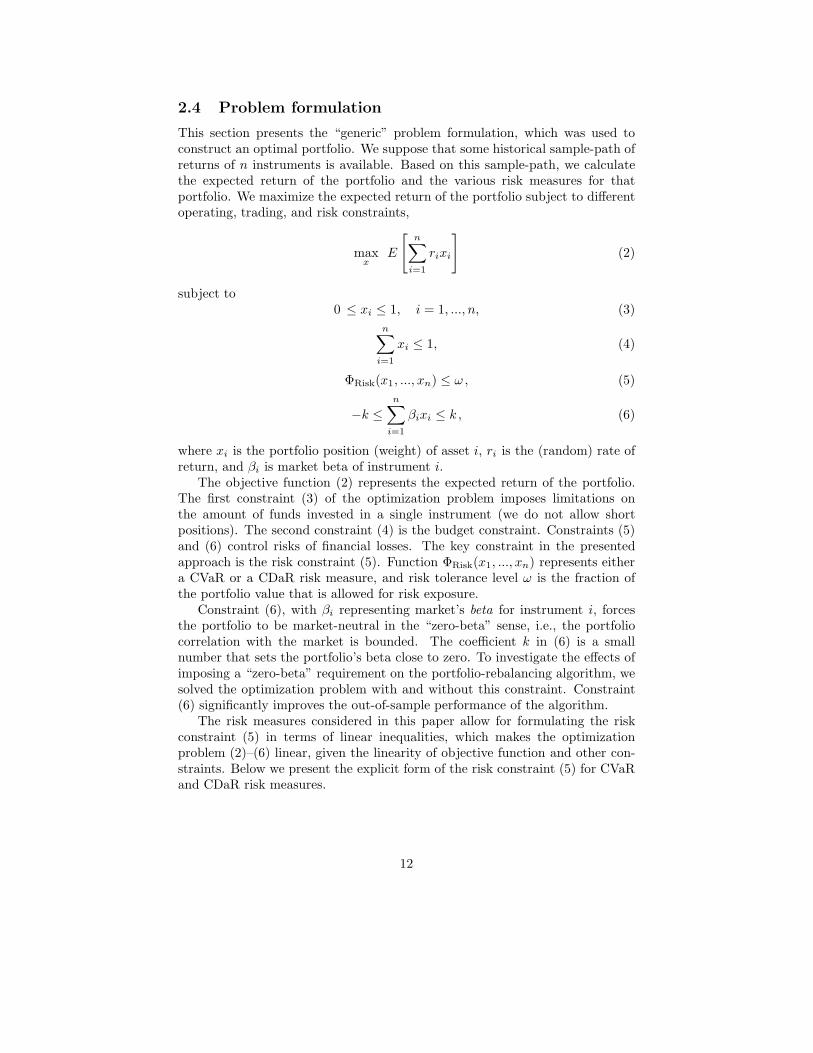
2.4 Problem formulation

This section presents the “generic” problem formulation, which was used toconstruct an optimal portfolio. We suppose that some historical sample-path ofreturns of n instruments is available. Based on this sample-path, we calculatethe expected return of the portfolio and the various risk measures for thatportfolio. We maximize the expected return of the portfolio subject to differentoperating, trading, and risk constraints,

maxx

E

[n∑

i=1

rixi

](2)

subject to0 ≤ xi ≤ 1, i = 1, ..., n, (3)

n∑i=1

xi ≤ 1, (4)

ΦRisk(x1, ..., xn) ≤ ω , (5)

−k ≤n∑

i=1

βixi ≤ k , (6)

where xi is the portfolio position (weight) of asset i, ri is the (random) rate ofreturn, and βi is market beta of instrument i.

The objective function (2) represents the expected return of the portfolio.The first constraint (3) of the optimization problem imposes limitations onthe amount of funds invested in a single instrument (we do not allow shortpositions). The second constraint (4) is the budget constraint. Constraints (5)and (6) control risks of financial losses. The key constraint in the presentedapproach is the risk constraint (5). Function ΦRisk(x1, ..., xn) represents eithera CVaR or a CDaR risk measure, and risk tolerance level ω is the fraction ofthe portfolio value that is allowed for risk exposure.

Constraint (6), with βi representing market’s beta for instrument i, forcesthe portfolio to be market-neutral in the “zero-beta” sense, i.e., the portfoliocorrelation with the market is bounded. The coefficient k in (6) is a smallnumber that sets the portfolio’s beta close to zero. To investigate the effects ofimposing a “zero-beta” requirement on the portfolio-rebalancing algorithm, wesolved the optimization problem with and without this constraint. Constraint(6) significantly improves the out-of-sample performance of the algorithm.

The risk measures considered in this paper allow for formulating the riskconstraint (5) in terms of linear inequalities, which makes the optimizationproblem (2)–(6) linear, given the linearity of objective function and other con-straints. Below we present the explicit form of the risk constraint (5) for CVaRand CDaR risk measures.

12

2.5 Conditional Value-at-Risk constraint

The loss function incorporated into CVaR constraint, is the negative portfolio’sreturn,

f(x,y) = −n∑

i=1

rixi, (7)

where the vector of instruments’ returns y = r = (r1, ..., rn) is random. Therisk constraint (5), φα(x) ≤ ω, where CVaR risk function replaces the functionΦRisk(x), is

ζ +1

(1 − α)J

J∑j=1

max

{0,−

n∑i=1

rijxi − ζ

}≤ ω, (8)

where rij is return of i-th instrument in scenario j, j = 1, ..., J . Since the lossfunction (7) is linear, the risk constraint (8) can be equivalently represented bythe linear inequalities,

ζ +1

1 − α

1J

J∑j=1

wj ≤ ω,

−n∑

i=1

rijxi − ζ ≤ wj , j = 1, ..., J, (9)

ζ ∈ R, wj ≥ 0, j = 1, ..., J.

This representation allows for reducing the optimization problem (2)–(6) withthe CVaR constraint to a linear programming problem.

2.6 Conditional Drawdown-at-Risk constraint

The CDaR risk constraint ∆α(x) ≤ ω has the form

η+1

1 − α

1J

J∑j=1

max

[0, max

1≤k≤j

{n∑

i=1

(k∑

s=1

ris

)xi

}−

n∑i=1

(j∑

s=1

ris

)xi − η

]≤ ω,

and it can be reduced to a set of linear constraints similarly to the CVaR con-straint.

3 Case study: portfolio of hedge funds

The case study investigates investment opportunities and tests portfolio man-agement strategies for a portfolio of hedge funds. Hedge funds are subject to lessregulations as compared with mutual or pension funds. Hence, very little infor-mation on hedge funds’ activities is publicly available (for example, many fundsreport their share prices only monthly). On the other hand, fewer regulations

13

and weaker government control provide more room for aggressive, risk-seekingtrading and investment strategies. As a consequence, the revenues in this in-dustry are on average much higher than elsewhere, but the risk exposure isalso higher (for example, the typical “life” of a hedge fund is about five years,and very few of them perform well in long run). Data availability and sizes ofdatasets impose challenging requirements on portfolio rebalancing algorithms.Also, the specific nature of hedge fund securities imposes some limitations onusing them in trading or rebalancing algorithms. For example, hedge fundsare far from being perfectly liquid: hedge funds may not be publicly tradedor may be closed to new investors. From this point of view, our results con-tain a rather schematic representation of investment opportunities existing inthe hedge fund market and do not give direct recommendations on investing inthat market. The goal of this study is to compare the recently developed riskmanagement approaches and to demonstrate their high numerical efficiency ina realistic setting.

The dataset for conducting the numerical experiments was provided to theauthors by the Foundation for Managed Derivatives Research. It contained amonthly data for more than 5000 hedge funds, from which we selected thosewith significantly long history and some minimum level of capitalization. Topass the selection, a hedge fund should have 66 months of historical data fromDecember 1995 to May 2001, and its capitalization should be at least 5 millionU.S. dollars at the beginning of this period. The total number of funds, whichsatisfied these criteria and accordingly constituted the investment pool for ouralgorithm, was 301. In this dataset, the field with the names of hedge funds wasunavailable; therefore, we identified the hedge funds with numbers, i.e., HF 1,HF 2, and so on. The historical returns from the dataset were used to generatescenarios for algorithm (2)–(6). Each scenario is a vector of monthly returns forall securities involved in the optimization, and all scenarios are assigned equalprobabilities.

We performed separate runs of the optimization problem (2)–(5), with andwithout constraint (6) with CVaR and CDaR risk measure in constraint (5),varying such parameters as confidence levels, risk tolerance levels etc.

The case study consisted from two sets of numerical experiments. The firstset of in-sample experiments included the calculation of efficient frontiers andthe analysis of the optimal portfolio structure for each of the risk measures. Thesecond set of experiments, out-of-sample testing, was designed to demonstratethe performance of our approach in a simulated historical environment.

3.1 In-sample results

Efficient frontier. For constructing the efficient frontier for the optimal port-folio with different risk constraints, we solved the optimization problem (2)–(5)with different risk tolerance levels ω in constraint (5), varied from ω = 0.005to ω = 0.25. The parameter α in CVaR and CDaR risk constraints was setto α = 0.90. The efficient frontier is presented in Figure 3, where the port-folio rate of return means expected yearly rate of return. In these runs, the

14

market-neutrality constraint (6) is inactive. For optimal portfolios, in the sense

Efficient Frontier with Zero-beta Constraint

30

33

36

39

42

45

0.5 1.5 2.5 3.5 4.5 5.5 6.5 7.5 8.5 9.5 10.5 11.5 12.5

Risk tolerance, %

Po

rtfo

lio

ra

te o

f re

turn

, %

CVaR

CDaRCDaR

CVaR

Figure 4: Efficient frontier for market-neutral portfolio with various risk con-straints (k = 0.01).

of problem (2)–(5), there exists an upper bound (equal to 48.13%) for the port-folio’s rate of return. Optimal portfolio with CVaR constraint reach this boundat about 18%-risk tolerance level, but the CDaR-constrained portfolio does notachieve the maximal expected return within the given range of ω values. CDaRis a relatively conservative constraint imposing requirements not only on themagnitude of loses, but also on the time sequence of losses (small consecutivelosses may lead to large drawdown, without a significant increase of CVaR).

Figure 4 presents efficient frontiers of optimal portfolio (2)–(5) with activemarket-neutrality constraint (6), where coefficient k equals to 0.01. Imposingthe extra constraint (6) causes a decrease in the in-sample optimal expectedreturn. For example, the “saturation” level of the portfolio’s expected return isnow 41.94%, and both portfolios reach that level at much lower values of risktolerance ω. However, the market-neutrality constraint almost does not affectthe curves of efficient portfolios in the leftmost points of efficient frontiers, whichcorrespond to the lowest values of risk tolerance ω.

Quite high rates of return for CVaR- and CDaR-efficient portfolios are ex-plained by the fact that 301 funds, selected to form the optimal portfolios,constitute about 6% of the initial hedge fund pool, and already are “the best ofthe best” in our data sample.

Optimal portfolio configuration. We now discuss the structure of theoptimal portfolio with various risk constraints. We selected those optimal port-folios on the efficient frontiers whose expected return is equal 35% (the market-neutrality constraint is not active).

Table 1 shows the configuration (portfolio weights) of the optimal portfolioswith CVaR and CDaR constraints. Among the 301 available instruments, only

15

Out-of-Sample: Portfolio with CVaR Constraints

0

100

200

300

400

500

600

Feb-9

7

May

-97

Aug

-97

Nov

-97

Feb-9

8

May

-98

Aug

-98

Nov

-98

Feb-9

9

May

-99

Aug

-99

Nov

-99

Feb-0

0

May

-00

Aug

-00

Nov

-00

Feb-0

1

Po

rtfo

lio

va

lue

, %

Figure 5: Historical trajectories of optimal portfolio with CVaR constraints.

few of them contribute to constructing the optimal portfolio. Moreover, a closerlook at Table 1 shows that nearly two thirds of the portfolio value for bothrisk measures is formed by three hedge funds HF 209, HF 219 and HF 231. Ingeneral, CVaR- and CDaR-optimal portfolios have quite similar structure.

Table 1: Portfolio weights for optimal portfolio with CVaR and CDaR con-straints.

HF49 HF84 HF93 HF100 HF126 HF169 HF196 HF209 HF219 HF231 HF258 HF259 HF298

CVaR 4.39% 0.00% 8.75% 7.37% 0.87% 1.01% 1.56% 22.47% 25.93% 16.92% 1.42% 8.94% 0.38%

CDaR 11.02% 4.19% 8.14% 6.63% 0.00% 5.43% 0.00% 21.47% 13.72% 18.30% 3.41% 5.87% 1.83%

3.2 Out-of-sample calculations

The out-of-sample testing of the portfolio optimization algorithm (2)–(6) shedslight on the “actual” performance of the approaches. The question is howwell the algorithms with different risk measures utilize the scenario informationbased on past history in producing a successful portfolio management strategy?An answer can be obtained, for instance, by interpreting the results of thepreceding section as follows: suppose we were back in May 2001, and we wouldlike to invest a certain amount of money in a portfolio of hedge funds to deliverthe highest reward under a specified risk level. Then, according to in-sampleresults, the best portfolio would be the one on the efficient frontier of a particularrebalancing strategy. In fact, such a portfolio offers the best return-to-risk ratio

16

provided that the historical distribution of returns will repeat in the future.To estimate the “actual” performance of the optimization approach, we used

part of the data for scenario generation, and the rest for evaluating the perfor-mance of the strategy.

We present the results of a “plain” out-of-sample test, where the older datais considered as the ‘in-sample’ data for the algorithm, and the newer data aretreated as “to-be-realized” future. First, we took the 12 monthly returns fromDecember 1995 to November 1996 as the initial historical data for constructingthe first portfolio to invest in, and observed the portfolio’s “realized” value byobserving the historical prices for December 1996. Then, we added one moremonth, December 1996, to the data which were used for scenario generation(12 months of historical data in total) to generate an optimal portfolio and toallocate to investments in January, 1997, and so on. Note that we did not imple-ment the “moving window” method for out-of-sample testing, where the samenumber of scenarios (i.e., the most recent historical points) is used for solvingthe portfolio-rebalancing problem. Instead, we accumulated the historical datafor portfolio optimization.

First, we perform the out-of-sample runs for each risk measure in constraint(5) for different values of risk tolerance level ω (market-neutrality constraint,(6), is inactive). Figures 5 and 6 illustrate the historical trajectories of the op-timal portfolio under different risk constraints (the portfolio values are givenin % relatively to the initial portfolio value). Risk tolerance level ω was set to0.005, 0.01, 0.03, 0.05, 0.10, 0.12, 0.15, 0.17 and 0.20, but for better readingof figures, we report only results with ω = 0.005, 0.01, 0.05, 0.10, and 0.15.The parameter α, which is risk confidence level in CDaR and CVaR constraintswas set to α = 0.90. Figures 7–8 shows that risk constraint (5) has a signifi-

Out-of-Sample: Portfolio with CDaR Constraints

0

100

200

300

400

500

600

Feb-9

7

May

-97

Aug-9

7

Nov

-97

Feb-9

8

May

-98

Aug-9

8

Nov

-98

Feb-9

9

May

-99

Aug-9

9

Nov

-99

Feb-0

0

May

-00

Aug-0

0

Nov

-00

Feb-0

1

Po

rtfo

lio

valu

e, %

Figure 6: Historical trajectories of optimal portfolio with CDaR constraints.

cant impact on the algorithm’s out-of-sample performance. Earlier, we had also

17

Out-of-sample: Portfolios with CVaR constraints

0

50

100

150

200

250

300

350

400

Feb-9

7

May

-97

Aug

-97

Nov

-97

Feb-9

8

May

-98

Aug

-98

Nov

-98

Feb-9

9

May

-99

Aug

-99

Nov

-99

Feb-0

0

May

-00

Aug

-00

Nov

-00

Feb-0

1

Po

rtfo

lio

valu

e, %

Figure 7: Historical trajectories of optimal portfolio with CVaR constraints.Lines with β = 0 correspond to portfolios with market-neutral constraint.

observed that this constraint has significant impact on the in-sample perfor-mance. Constraining risk in the in-sample optimization decreases the optimalvalue of the objective function, and the results reported in the preceding subsec-tion reflect this. The risk constraints force the algorithm to favor less profitablebut safer decisions over more profitable but “dangerous” ones. Imposing extraconstraints always reduces the feasibility set, and consequently leads to loweroptimal objective values. However, the situation changes dramatically for anout-of-sample application of the optimization algorithm. The numerical exper-iments show that constraining risks improves the overall performance of theportfolio rebalancing strategy in out-of-sample runs; tighter in-sample risk con-straint may lead to both lower risks and higher out-of-sample returns. For bothrisk measures, loosening the risk tolerance (i.e., increasing ω values) results in anincreased volatility of the out-of-sample portfolio returns and, after exceedingsome threshold value, in degradation of the algorithm’s performance, especiallyduring the last 13 months (March 2000 – May 2001). For all risk functions inconstraint (5), the most attractive portfolio trajectories are obtained for risktolerance level ω = 0.005, which means that these portfolios have high returns(high final portfolio value), low volatility, and low drawdowns. Increasing ω to0.01 leads to a slight increase of the final portfolio value, but it also increasesportfolio volatility and drawdowns, especially for the second quarter of 2001.For larger values of ω the portfolio returns deteriorate, and for all risk measuresportfolio curves with ω = 0.10 show quite poor performance. Further increas-ing the risk tolerance to ω = 0.15 in some cases allows for achieving higherreturns at the end of 2000, but after this high peak the portfolio suffers severedrawdowns.

Figures 7 and 8 illustrate the effects of imposing market-neutrality con-

18

straint (6) in addition to risk constraint (5). The primary purpose of (6) ismaking the portfolio uncorrelated with market. The main idea of composinga market-neutral portfolio is protecting it from market drawdowns. Figures7–8 compare the trajectories of market-neutral and without risk-neutrality op-timal portfolios. Additional constraining resulted in most cases in a furtherimprovement of the portfolio’s out-of-sample performance. To clarify how therisk-neutrality condition (6) influences the portfolio’s performance, we displayedonly figures for lowest and highest values of the risk tolerance parameter, namelyfor ω = 0.005 and ω = 0.20. Coefficient k in (6) was set to k = 0.01, and instru-ments’ betas βi were calculated by correlating with the benchmark S&P 500index. For portfolios with tight risk constraints (ω = 0.005) imposing market-neutrality constraint (6) straightened their trajectories (reduced volatility anddrawdowns), which made the historic curves almost monotone curves with a pos-itive slope. On top of that, portfolios with market-neutrality constraint had ahigher final portfolio value, compared to those without market-neutrality. Also,for portfolios with loose risk constraints (ω = 0.20) imposing market-neutralityconstraint had a positive effect on the form of their trajectories, dramaticallyreducing volatility and drawdowns.

Out-of-Sample: Portfolios with CDaR Constraints

0

50

100

150

200

250

300

350

400

Feb-9

7

May

-97

Aug

-97

Nov

-97

Feb-9

8

May

-98

Aug

-98

Nov

-98

Feb-9

9

May

-99

Aug

-99

Nov

-99

Feb-0

0

May

-00

Aug

-00

Nov

-00

Feb-0

1

Po

rtfo

lio

va

lue

, %

Figure 8: Historical trajectories of optimal portfolio with CDaR constraints.Lines with β = 0 correspond to portfolios with market-neutral constraint.

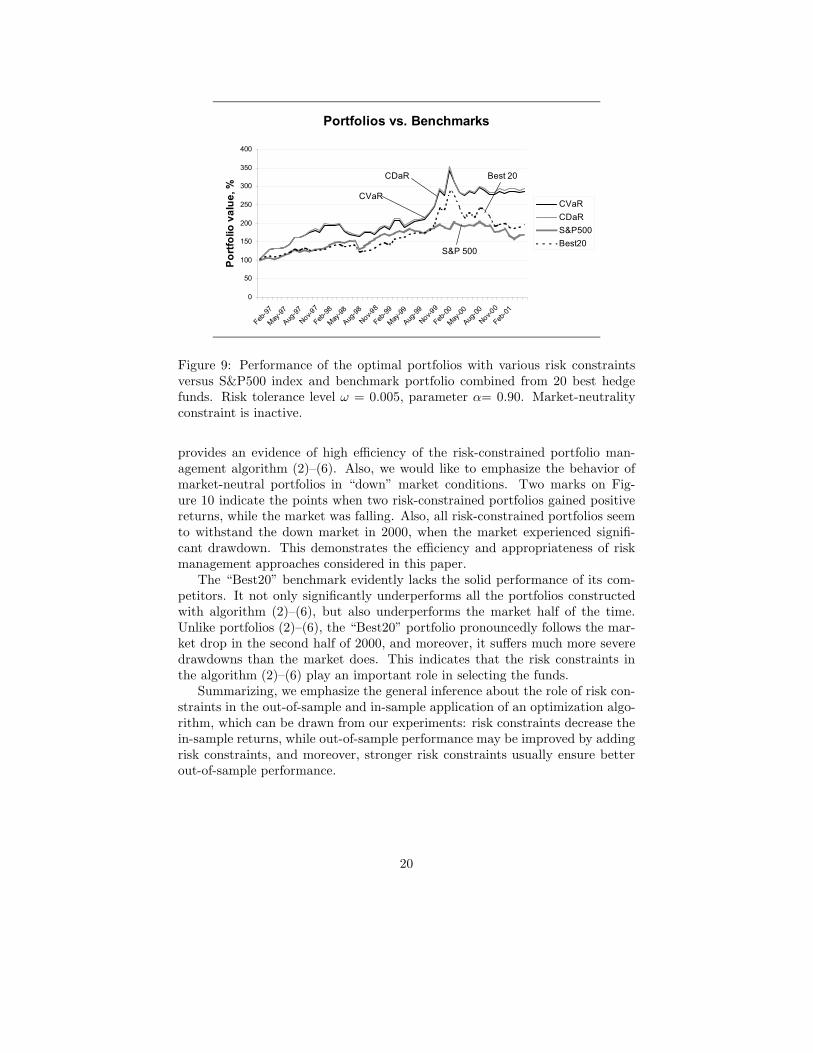
Finally, Figures 9 and 10 demonstrate the performance of the optimal port-folios versus two benchmarks: 1) S&P500 index; 2) “Best20”, representing theportfolio distributed equally among the “best” 20 hedge funds. These 20 hedgefunds include funds with the highest expected monthly returns calculated withpast historical information. Similarly to the optimal portfolios (2)–(6), the“Best20” portfolio was monthly rebalanced (without risk constraints).

According to Figures 9–10, CVaR and CDaR constrained portfolios, bothwithout and with market-neutrality condition, outperform benchmarks, which

19

Portfolios vs. Benchmarks

0

50

100

150

200

250

300

350

400

Feb-9

7

May

-97

Aug

-97

Nov-

97

Feb-9

8

May

-98

Aug

-98

Nov-

98

Feb-9

9

May

-99

Aug

-99

Nov-

99

Feb-0

0

May

-00

Aug

-00

Nov-

00

Feb-0

1

Po

rtfo

lio

va

lue

, %

CVaR

CDaR

S&P500

Best20

CVaR

S&P 500

CDaR Best 20

Figure 9: Performance of the optimal portfolios with various risk constraintsversus S&P500 index and benchmark portfolio combined from 20 best hedgefunds. Risk tolerance level ω = 0.005, parameter α= 0.90. Market-neutralityconstraint is inactive.

provides an evidence of high efficiency of the risk-constrained portfolio man-agement algorithm (2)–(6). Also, we would like to emphasize the behavior ofmarket-neutral portfolios in “down” market conditions. Two marks on Fig-ure 10 indicate the points when two risk-constrained portfolios gained positivereturns, while the market was falling. Also, all risk-constrained portfolios seemto withstand the down market in 2000, when the market experienced signifi-cant drawdown. This demonstrates the efficiency and appropriateness of riskmanagement approaches considered in this paper.

The “Best20” benchmark evidently lacks the solid performance of its com-petitors. It not only significantly underperforms all the portfolios constructedwith algorithm (2)–(6), but also underperforms the market half of the time.Unlike portfolios (2)–(6), the “Best20” portfolio pronouncedly follows the mar-ket drop in the second half of 2000, and moreover, it suffers much more severedrawdowns than the market does. This indicates that the risk constraints inthe algorithm (2)–(6) play an important role in selecting the funds.

Summarizing, we emphasize the general inference about the role of risk con-straints in the out-of-sample and in-sample application of an optimization algo-rithm, which can be drawn from our experiments: risk constraints decrease thein-sample returns, while out-of-sample performance may be improved by addingrisk constraints, and moreover, stronger risk constraints usually ensure betterout-of-sample performance.

20

Market-Neutral Portfolios vs. Bencmarks

0

50

100

150

200

250

300

350

400

Feb-9

7

May

-97

Aug

-97

Nov-

97

Feb-9

8

May

-98

Aug

-98

Nov-

98

Feb-9

9

May

-99

Aug

-99

Nov-

99

Feb-0

0

May

-00

Aug

-00

Nov-

00

Feb-0

1

Po

rtfo

lio

va

lue

, %

CVaR

CDaR

S&P500

Best20

CVaR

S&P 500

CDaR

Best 20

Figure 10: Figure 10. Performance of market-neutral optimal portfolio withvarious risk constraints versus S&P500 index and benchmark portfolio combinedfrom 20 best hedge funds. Risk tolerance level is ω = 0.005, parameter is α=0.90.

4 Conclusions

We tested the performance of a portfolio allocation algorithm with differenttypes of risk constraints in an application for managing a portfolio of hedgefunds. As the risk measure in the portfolio optimization problem, we usedConditional Value-at-Risk and Conditional Drawdown-at-Risk. We combinedthese risk constraints with the market-neutrality (zero-beta) constraint makingthe optimal portfolio uncorrelated with the market.

The numerical experiments consist of in-sample and out-of-sample testing.We generated efficient frontiers and compared algorithms with various con-straints. The out-of-sample part of experiments was performed in two setups,which differed in constructing the scenario set for the optimization algorithm.

The results obtained are dataset-specific and we cannot make direct recom-mendations on portfolio allocations based on these results. However, we learnedseveral lessons from this case study. Imposing risk constraints may significantlydegrade in-sample expected returns while improving risk characteristics of theportfolio. In-sample experiments showed that for tight risk tolerance levels, allrisk constraints produce relatively similar portfolio configurations. Imposingrisk constraints may improve the out-of-sample performance of the portfolio-rebalancing algorithms in the sense of risk-return tradeoff. Especially promisingresults can be obtained by combining several types of risk constraints. In partic-ular, we combined the market-neutrality (zero-beta) constraint with CVaR orCDaR constraints. We found that tightening of risk constraints greatly im-proves portfolio dynamic performance in out-of-sample tests, increasing the

21

overall portfolio return and decreasing both losses and drawdowns. In addition,imposing the market-neutrality constraint adds to the stability of portfolio’sreturn, and reduces portfolio drawdowns. Both CDaR and CVaR risk measuresdemonstrated a solid performance in out-of-sample tests.

We thank the Foundation for Managed Derivatives Research for providingthe dataset for conducting numerical experiments and partial financial supportof this case study.

References

[1] Acerbi, C., Nordio, C. and C. Sirtori (2001): Expected shortfall asa tool for financial risk management. Working paper, (download fromhttp://www.gloriamundi.org).

[2] Acerbi, C., and D. Tasche (2001): On the coherence of expected shortfall.Working paper, (download from http://www.gloriamundi.org).

[3] Ackermann, C., McEnally, R., and D. Ravenscraft (1999) “The Perfor-mance of Hedge Funds: Risk, Return and Incentives”, Journal of Finance,54, 833–874.

[4] Amin, G., and H. Kat (2001) “Hedge Fund Performance 1990–2000: Dothe ‘Money Machines’ Really Add Value?”, Working paper.

[5] Andersson, F., Mausser, H., Rosen, D., and S. Uryasev (2001) “CreditRisk Optimization with Conditional Value-at-Risk Criterion”, Mathemat-ical Programming, Series B 89, 273-291.

[6] Artzner, P., Delbaen F., Elber, J. M., and D. Heath (1997) “ThinkingCoherently”, Risk, 10, 68–71.

[7] Artzner, P., Delbaen F., Elber, J. M., and D. Heath (1999) “CoherentMeasures of Risk”, Mathematical Finance, 9, 203–228.

[8] BARRA RogersCasey (2000) Market Neutral Investing.

[9] Brown, S., and W. Goetzmann (2000) “Hedge Funds with Style”, YaleInternational Center for Finance, working paper No. 00-29.

[10] Carino, D. R., and W. T. Ziemba (1998) “Formulation of the RussellYasuda Kasai Financial Planning Model”, Operations Research, 46 (4),433–449.

[11] Carino, D. R., Myers D. H., and W. T. Ziemba (1998) “Concepts, Tech-nical Issues and Uses of the Russell-Yasuda Kasai Model” Operations Re-search, 46 (4), 450–462.

[12] Chekhlov, A., Uryasev, S., and M. Zabarankin (2000) “Portfolio Optimiza-tion with Drawdown Constraints”, Research Report 2000-5. ISE Dept.,Univ. of Florida.

22

[13] Consigli, G., and M. A. H. Dempster (1997) “Solving dynamic portfo-lio problems using stochastic programming”, Zeitschrift fur AngewandteMathematik und Mechanik, 775, 565–566.

[14] Consigli, G., and M. A. H. Dempster (1998) “Dynamic stochastic program-ming for asset-liability management”, Annals of Operations Research, 81,131–161.

[15] Dembo, R., and A. King (1992) “Tracking Models and the Optimal RegretDistribution in Asset Allocation”, Applied Stochastic Models and DataAnalysis, 8, 151–157.

[16] Duarte, A. Jr. (1999) “Fast computation of efficient portfolios”, Journalof Risk, 1 (4), 1–24.

[17] Duffie, D. and J. Pan (1997) “An Overview of Value-at-Risk”, Journal ofDerivatives, 4, 7–49.

[18] Embrechts P., McNeil, A.. and D. Straumann (2001) Correlation and De-pendency in Risk Management: Properties and Pitfalls, M. Dempster(Ed.) in ”Risk Management: Value at Risk and Beyond,.” CambridgeUniversity Press, Cambridge.

[19] Fung, W., and D. Hsieh (1997) “Empirical Characteristics of DynamicTrading Strategies: The Case of Hedge Funds”, Review of Financial Stud-ies, 10 (2), 275–302.

[20] Fung, W., and D. Hsieh (2000) “Performance Characteristics of HedgeFunds and Commodity Funds: Natural vs. Spurious Biases”, Journal ofFinancial and Quantitative Analysis, 35, 291–307.

[21] Fung, W., and D. Hsieh (2001) “The Risk in Hedge Fund Strategies:Theory and Evidence from Trend Followers”, Review of Financial Studies,14, 313–341.

[22] Harlow, W. V. (1991) “Asset Allocation in a Downside-Risk Framework”,Financial Analysts Journal, Sep/Oct, 28–40.

[23] Jorion, P. (1997) Value-at-Risk: The New Benchmark for ControllingMarket Risk, McGraw-Hill, New York.

[24] Konno, H., and S. Shirakawa (1994) “Equilibrium Relations in a CapitalAsset Market: a Mean Absolute Deviation Approach”, Financial Engi-neering and the Japanese Markets, 1, 21–35.

[25] Konno, H., and A. Wijayanayake (1999) “Mean-Absolute Deviation Port-folio Optimization Model Under Transaction Costs”, Journal of the Op-erations Research Society of Japan, 42 (4), 422–435.

23

[26] Konno, H., and H. Yamazaki (1991) “Mean Absolute Deviation PortfolioOptimization Model and Its Application to Tokyo Stock Market”, Man-agement Science, 37, 519–531.

[27] Krokhmal, P., Palmquist, J., and S. Uryasev (2002) “Portfolio Optimiza-tion with Conditional Value-At-Risk Objective and Constraints”, Journalof Risk, 4 (2).

[28] Kusy, M. I., and W. T. Ziemba (1986) “A Bank Asset and Liability Man-agement Model”, Operations Research, 34 (3), 356–376.

[29] Lhabitant, F.-S. (2001) “Assessing Market Risk for Hedge Funds andHedge Funds Portfolios”, Research Paper No 24, Union Bancaire Privee.

[30] Lo, A. (2001) “Risk Management for Hedge Funds: Introduction andOverview”, Financial Analysts Journal, 57(6), 16–33.

[31] Markowitz, H. M. (1952) “Portfolio selection”, Journal of Finance, 7 (1),77–91.

[32] Markowitz, H. M. (1991) Portfolio Selection: Efficient Diversification ofInvestments, Blackwell, New York.

[33] Mausser, H., and D. Rosen (1998) “Beyond VaR: From Measuring Riskto Managing Risk”, ALGO Research Quarterly, 1 (2), 5–20.

[34] Rockafellar, R. T. (1970) “Convex Analysis” Princeton Mathematics, Vol.28, Princeton Univ. Press.

[35] Rockafellar, R. T., and S. Uryasev (2000) “Optimization of ConditionalValue-at-Risk”, Journal of Risk, 2, 21–41.

[36] Rockafellar, R. T., and S. Uryasev (2002) “Conditional Value-at-Risk forGeneral Loss Distributions”, Journal of Banking and Finance, 26, 1443–1471.

[37] Pritsker, M. (1997) “Evaluating Value-at-Risk Methodologies”, Journalof Financial Services Research, 12 (2/3), 201–242.

[38] Ogryczak, W. and A. Ruszczynski (1999) “From Stochastic Dominance toMean-Risk Model”, European J. of Operational Research, 116, 33–50.

[39] Staumbaugh, F. (1996) “Risk and Value-at-Risk”, European ManagementJournal, 14 (6), 612–621.

[40] Testuri, C., and S. Uryasev (2000) “On Relation Between Expected Re-gret and Conditional Value-at-Risk”, Research Report 2000-9. ISE Dept.,Univ. of Florida.

24

[41] Turner A. L., Stacy C., Carino D. R., David H. Myers D. H., WatanabeK., Sylvanus M., Terry Kent T., and W. T. Ziemba (1994) “The Russell-Yasuda Kasai Model: An Asset/Liability Model for a Japanese InsuranceCompany Using Multistage Stochastic Programming”, Interfaces, 24 (1),29–49.

[42] Young, M. R. (1998) “A Minimax Portfolio Selection Rule with LinearProgramming Solution”, Management Science, 44 (5), 673–683.

[43] Zenios, S. A. (1993) “A Model for Portfolio Management with Mortgage-Backed Securities”, Annals of Operations Research, 43, 337–356.

[44] Zenios, S. A. (1999) “High Performance Computing for Financial Plan-ning: The Last Ten Years and the Next”, Parallel Computing, 25, 2149–2175.

[45] Ziemba, W. T., and R. G. Vickson (1975) Stochastic Optimization Modelsin Finance, Academic Press, New York.

[46] Ziemba, W. T., Ed. (2002) The Stochastic Programming Approach to As-set, Liability and Wealth Management, AIMR-Blackwell, in press.

[47] Ziemba, W. T. and M. J. Mulvey, Eds (1998) “Worldwide Asset and Lia-bility Modeling”, Cambridge University Press, Publications of the NewtonInstitute.

25