Embed Size (px)
Citation preview
1
Circuit Simulation via Matrix Exponential Operators
CK ChengUC San Diego

2
Outline
• General Matrix Exponential• Krylov Space and Arnoldi Orthogonalization
• Matrix Exponential Method– Krylov Subspace Approximation– Invert Krylov Subspace Approximation– Rational Krylov Subspace Approximation

3
General Matrix Exponential
• 𝝓0(At)= eAt• 𝝓1(At)= d𝞽=A-1(eAt-I)• 𝝓2(At)= 𝞽d𝞽=A-2(eAt-A-I)• 𝝓k(At)=Exercise: Expand the right hand side expression to remove the inverse operation.

4
Krylov Space and Arnoldi Orthonormalization
Input A and v1=x0/|x0|
Output AV=VH+hm+1vm+1emT
For i=1, …, m• Ti+1=Avi
• For j=1, …, I– hji=<Ti+1,vj>
– Ti+1=Ti+1-hjivj
• End For• hi+1,i=|Ti+1|
• vi+1=1/hi+1 Ti+1
End For
In other words,Avi-=hi+1,ivi+1

5
Standard Krylov Space
Generate: AV=VH+hm+1vm+1emT
Thus, we have eAhv1≈VeHhe1
Residual r=Cdx/dt-Gx=-hm+1Cvm+1emTeHhe1
Derivation:Cdx/dt-Gx=CVHeHhe1-GVeHhe1
=(CVH-GV)eHhe1 = C(VH-C-1GV)eHhe1
=C(VH-VH-hm+1vm+1emT)eHhe1
=-hm+1Cvm+1emTeHhe1

6
Standard Mexp
Error trend
12
hhError e e e mHAmv v V
sweep m and h

7
Invert Krylov Space
Generate: A-1V=VH+hm+1vm+1emT
Let H=H-1, we have eAhv1≈VeHhe1
Residual r=Cdx/dt-Gx=hm+1Gvm+1emTHeHhe1
Derivation:Cdx/dt-Gx=CVHeHhe1-GVeHhe1
=(CVH-GV)eHhe1 = G(G-1CVH-V)eHhe1
=G(A-1VH-V)eHhe1
=hm+1Gvm+1emTHeHhe1

8
• large step size with less dimensionInvert Matrix Exponential
sweep m and h1
12
hherror e e e
mHA
mv v V

9
Rational Krylov SpaceGenerate: (1-rA)-1V=VH+hm+1vm+1em
T
Let H=1/r (I-H-1) we have eAhv1≈VeHhe1
Residual r=Cdx/dt-Gx=-hm+1(C/r-G)vm+1emTH-1eHhe1
Derivation:Cdx/dt-Gx=CVHeHhe1-GVeHhe1
=(CVH-GV)eHhe1 = (1/r CV(I-H-1)-GV)eHhe1
=(1/rCV(H-1)-GVH)H-1eHhe1
=((1/rC-G)VH-1/rCV)H-1eHhe1
=-hm+1(C/r-G)vm+1emTH-1eHhe1

10
• large step size with less dimensionRational Matrix Exponential
fix , sweep m and h 1
~
2eeeError
hh mH
mA Vvv

11
Different
needs large m

12
Different

13
Spectral Transformation – = 10f• Small RC mesh, 100 by 100• Different h for Krylov subspace• Different for rational Krylov subspace

14
Spectral Transformation– = 1p• Small RC mesh, 100 by 100• Different h for Krylov subspace• Different for rational Krylov subspace

15
Spectral Transformation– = 100p• Small RC mesh, 100 by 100• Different h for Krylov subspace• Different for rational Krylov subspace

16
Sweep for Large Range

17
Sweep for Large Range
18
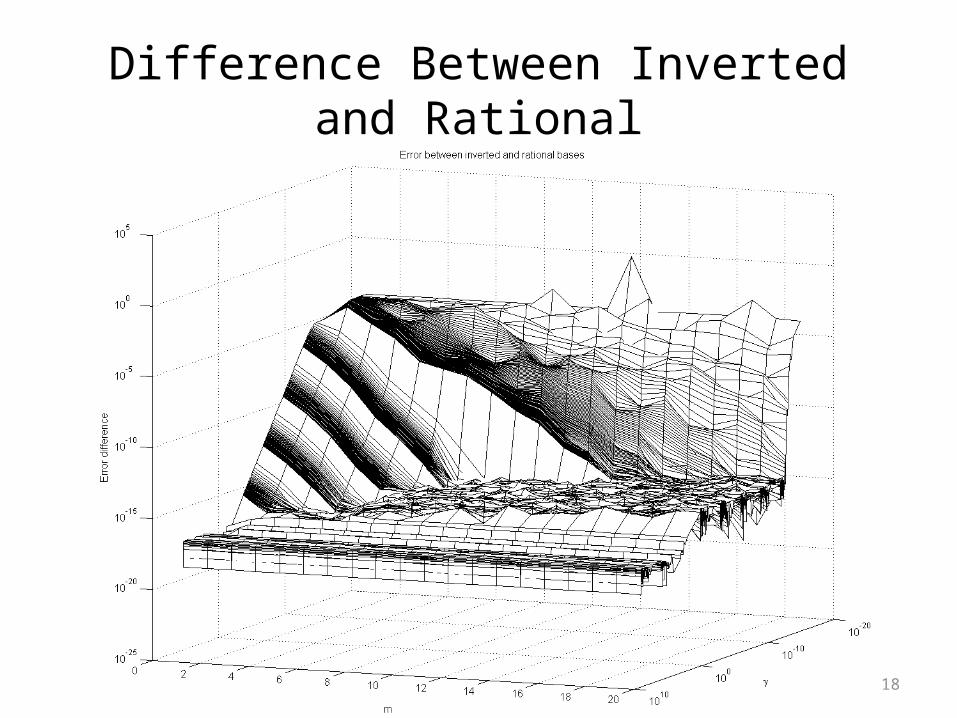
Difference Between Inverted and Rational
19
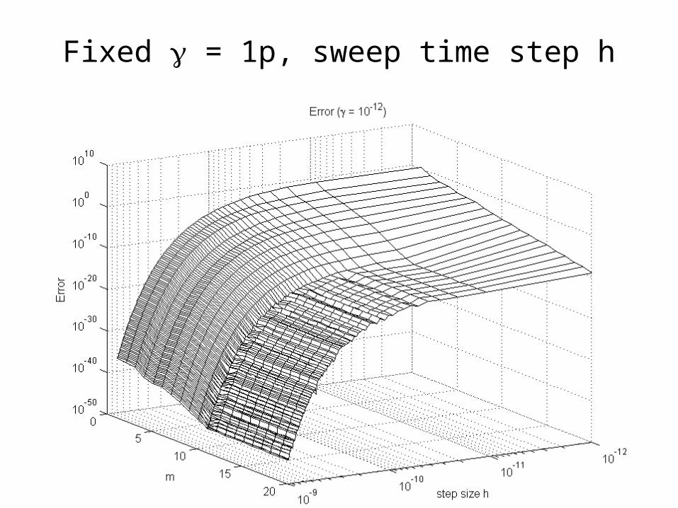
Fixed = 1p, sweep time step h

20
Fixed = 1n, sweep time step h

21
Fixed = 1u, sweep time step h

22
Fixed = 1m, sweep time step h

23
Fixed = 1, sweep time step h

24
Fixed = 1k, sweep time step h

25
Fixed = 1M, sweep time step h

26
Krylov Space ResidualGenerate: AV=VH+hm+1vm+1em
T
Thus, we have eAhv1≈VeHhe1
Residual r=Cdx/dt-Gx=-hm+1Cvm+1emTeHhe1
Derivation:1. Set Y=[e1 He1 H2e1 … Hm-1e1]
2. We have YC=HY where C=zm+cm-1zm-1+…+c1z+c0=0
has roots 𝞴1, 𝞴2,… 𝞴m
0 -c0
1 0 -c1
1 0 -c2
… … …1 0 -cm-2
1 -cm-1

27
Krylov Space ResidualResidual r=Cdx/dt-Gx=-hm+1Cvm+1em
TeHhe1
3. C=V-1DV (VC=DV), V= D=Diag(𝞴1, 𝞴2,… 𝞴m)
4. H=YCY-1=YV-1DVY-1
5. eH=YV-1eDVY-1
6. emTeHhe1
=emTYV-1eDhVY-1e1
=emTYV-1eDh1, 1=[1,1,…1]T
=emTYV-1[e𝞴1h, e𝞴2h,…,e𝞴mh]T ≈hm-1/(m-1)!
1 𝞴1 . 𝞴1m-11 𝞴2 . 𝞴2m-1. . . .. . . .. . .
1 𝞴m . 𝞴mm-1
28
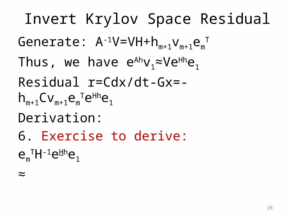
Invert Krylov Space ResidualGenerate: A-1V=VH+hm+1vm+1em
T
Thus, we have eAhv1≈VeHhe1
Residual r=Cdx/dt-Gx=-hm+1Cvm+1emTeHhe1
Derivation:6. Exercise to derive: em
TH-1eHhe1≈