Channel estimation in multiple-input multiple-output systems

CHANNEL ESTIMATION IN MULTIPLE-INPUT MULTIPLE-OUTPUTSYSTEMS

By

BEOMJIN PARK

A DISSERTATION PRESENTED TO THE GRADUATE SCHOOLOF THE UNIVERSITY OF FLORIDA IN PARTIAL FULFILLMENT

OF THE REQUIREMENTS FOR THE DEGREE OFDOCTOR OF PHILOSOPHY

UNIVERSITY OF FLORIDA

2004

Copyright 2004

by

Beomjin Park

To my parents, Kyung-Ho Park and Bong-Hee Kong.

ACKNOWLEDGMENTS

First of all, I would like to thank my advisor, Dr. Tan F. Wong, for his energetic

and passionate guidance throughout my Ph.D. program. Without his continuous and

patient guidance, this work never would have been accomplished.

I would also like to thank Dr. Yuguang “Michael” Fang, Dr. John M. Shea, and

Dr. Louis N. Cattafesta III for their supporting roles as my committee members.

Last but not least, I would like to thank my family for always encouraging and

trusting me throughout my whole life. Their endless support encouraged me to finish

this valuable accomplishment.

IV

TABLE OF CONTENTSpage

ACKNOWLEDGMENTS iv

LIST OF TABLES vii

LIST OF FIGURES viii

ABSTRACT x

CHAPTER

1 INTRODUCTION 1

1.1 Previous Work 3

1.2 Problem Approach 6

1.3 Organization of This Dissertation 7

2 BACKGROUND 9

2.1 Space-Time Wireless Communication Systems 9

2.1.1 Space-Time Signal Model 9

2.1.2 MIMO Channel Model 10

2.2 Minimum Variance Unbiased Estimation 14

2.2.1 Unbiased Estimator 14

2.2.2 Minimum Variance Criterion 15

2.2.3 Linear Models 15

2.2.4 Best Linear Unbiased Estimator 17

2.2.5 Maximum Likelihood Estimator 20

2.3 Bayesian Estimator 21

2.4 Circulant Matrices and Toeplitz Matrices 23

2.4.1 Circulant Matrices 24

2.4.2 Toeplitz Matrices 25

2.4.3 Absolutely Summable Toeplitz Matrix 26

2.5 Summary 29

3 SYSTEM MODEL AND CHANNEL ESTIMATION 30

3.1 Channel Estimation with BLUE 30

3.1.1 System Model 30

3.1.2 Best Linear Unbiased Channel Estimator 32

3.2 Channel Estimation with Bayesian Estimator 38

3.2.1 System Model 38

v

3.2.2

Bayesian Channel Estimator 39

3.3 Summary 43

3.4 Derivation of the J Matrix 43

4 TRAINING SEQUENCE OPTIMIZATION 48

4.1 Optimal Training Sequence Set with BLUE 48

4.2 Optimal Training Sequence Set with Bayesian Estimator 51

4.3 Conclusion 54

4.4 Solution of the Optimization Problem 54

5 FEEDBACK DESIGN 58

5.1 Feedback Design for BLUE 58

5.2 Feedback Design for Bayesian Estimator 60

5.3 Summary 63

6 NUMERICAL RESULTS 64

6.1 Asymptotic Estimation Performance Gain 64

6.1.1 BLUE 64

6.1.2 Bayesian Estimatior 66

6.2 Numerical Examples for BLUE 67

6.2.1 AR(1) Jammer 68

6.2.2 Co-channel Interferer 72

6.2.3 Average MSE with Hadamard Sequence Set 77

6.3 Numerical Examples for Bayesian Estimator 83

6.3.1 AR(1) Jammer 83

6.3.2 Co-channel interferer 84

6.3.3 Bit Error Rate Performance 92

6.4 Conclusion 92

7 CONCLUSION AND FUTURE WORK 96

7.1 Conclusion 96

7.2 Future Work 97

REFERENCES 100

BIOGRAPHICAL SKETCH 103

vi

TableLIST OF TABLES

page

3-1 Matrix Notation 47

6-1 Comparison of asymptotic maximum MSE reduction ratio and MSEratio between using optimal and Hadamard sequences in the case of

AR jammers 95

6-2 Comparison of asymptotic maximum MSE reduction ratio and MSEratio between using optimal and Hadamard sequences in the case of

co-channel interferers 95

vii

LIST OF FIGURESFigure page

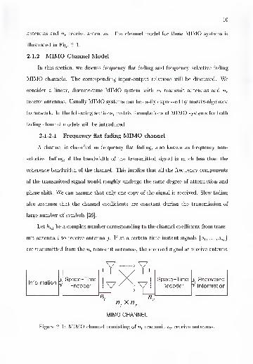
2-1 MIMO channel consisting of nt transmit nr receive antennas 10

2-2 Block transmission [24] 13

2-3 Definition of time index for the block transmission [24] 13

6-1 Comparison of MSEs obtained by using different training sequence sets.

AR-1 jammer with a = 0.7 and n t= nr = 2 70


AR-1 jammer with a = 0.9 and n t = nr = 2 71


Co-channel interferer with rectangular waveform, r = 0.3T, and

n t — nr = 2 75


Co-channel interferer with rectangular waveform, r = 0.5T, and

nt = nr = 2 76


Co-channel interferer with raised-cosine waveform, /? = 0.5, r =0.3T, and nt — nr = 2 78


Co-channel interferer with raised-cosine waveform, (5 = 0.5, r =0.5T, and nt = nr — 2 79

6-7 Comparison MSEs obtained by using optimal training sequence set

with average MSEs obtained by using all possible Hadamard training

sequence set. AR(1) jammer with a — 0.7 and nt = nr = 2 80



sequence set. AR(1) jammer with a = 0.9 and n t = nr — 2 81



sequence set. Co-channel interferer with rectangular waveform, r =0.3T and n t = n r = 2

viii

82


Two AR(1) interferers with cq = 0.3 and a2 = 0.5 85


Two AR(1) interferers with cq = 0.7 and a2 — 0.9 86


Two co-channel interferers with rectangular waveforms and delays

n = 0.3T, t2 = 0.5T 89


Two co-channel interferers with ISI-free waveform waveforms and

delays T\ = 0.3T, t2 = 0.5T 91

6-14 Comparison of BERs obtained by using different training sequence sets.


6-15 Comparison of BERs obtained by using different training sequence sets.


IX

Abstract of Dissertation Presented to the Graduate School

of the University of Florida in Partial Fulfillment of the

Requirements for the Degree of Doctor of Philosophy

CHANNEL ESTIMATION IN MULTIPLE-INPUT MULTIPLE-OUTPUTSYSTEMS

By

Beomjin Park

May 2004

Chair: Tan F. WongMajor Department: Electrical and Computer Engineering

We address the problems of channel estimation and optimal training sequence

design for multiple-input and multiple-output (MIMO) systems over flat fading chan-

nels in the presence of colored interference. In practice, information of the unknown

channel parameters is often obtained by sending known training symbols to the re-

ceiver. During the training period, we obtain the estimates of the channel parameters

based on the received training block. This method is called training based channel

estimation. In order to estimate unknown channel parameters, we employ two dif-

ferent channel estimators - the best linear unbiased estimator (BLUE) and Bayesian

channel estimator. We consider the BLUE for the case where there is a single inter-

ferer with the deterministic channel assumption. We consider the Bayesian channel

estimator for the case where there are multiple interferers with the assumption of

random channels. We note that the mean square error (MSEs) of the channel esti-

mators are dependent on the choice of the training sequence set. Hence we determine

the optimal training sequence set that can minimize the MSEs of the channel esti-

mators under a total transmit power constraint. In order to obtain the advantage of

x

the optimal training sequence design, long-term statistics of the interference corre-

lation are needed at the transmitter. Hence this information needs to be estimated

at the receiver and fed back to the transmitter. It is desirable that if we can reduce

the estimation error of the short-term channel fading parameters by using a minimal

amount of information that is fed back from the receiver. We develop such a feedback

strategy to design an approximate optimal training sequence set in this work.

xi

CHAPTER 1

INTRODUCTION

With the emergence of next-generation wireless mobile communications, there

is an increasing demand for higher data rates, better quality of service, and higher

network capacity. In an effort to support such demand within the limited availability

of radio frequency spectrum, many researchers have begun to utilize not only the

time and frequency dimensions but also the space dimension to design communica-

tion systems with higher spectral efficiencies. Recent research in information theory

has shown that large gains in reliability of communications over wireless channels

can be achieved by exploiting spatial diversity [1, 2]. The concept of spatial diver-

sity is that, in the presence of random fading caused by multi-path propagation, the

signal-to-noise ratio (SNR) can be significantly improved by combining the outputs

of decorrelated antenna elements. Such space utilization can be usually obtained by

using multiple antenna elements arranged in an array at both the transmitter and

receiver. Furthermore, it has been reported that multiple antennas along with space-

time coding (STC) or diversity techniques can aggressively exploit multi-path propa-

gation effects for the benefit of improving the communication capability of a system.

Recently, wireless communication systems using multiple antennas, usually referred

to as multiple-input multiple-output (MIMO) systems, have drawn considerable at-

tention, because MIMO systems promise higher capacity [1, 2] than single-antenna

systems over fading channels. As described in Gesbert et al. [3], the idea behind

MIMO is that the signals on the transmit antennas at one end and the receive an-

tennas at the other end are “combined” in such a way that the quality (bit-error rate

or BER) or the data rate (bits/sec) of communication for each MIMO user will be

improved. Different STC techniques [4-8] have been proposed to practically achieve

1

2

the capacity advantages of MIMO systems. STC is a set of practical signal design

techniques aimed at approaching the information theoretic capacity limit of MIMO

channels. The fundamentals of STC were established by Tarokh et al. in 1998 [4],

Among STC techniques, the main classes are Bell Labs layered space-time (BLAST)

architecture proposed by Foschini [1], space-time trellis codes (STTC) proposed by

Tarokh et al. [4], and space-time block codes (STBC) proposed by Alamouti [8].

Moreover major impairments such as fading, delay spread, and co-channel in-

terference caused by the wireless communication channels can be further mitigated

by employing MIMO systems. In a multi-path fading environment, the transmitted

signal is scattered by objects such as buildings, trees, or mountains before reaching

the receiver. This causes the signal to fade. While this scattering is detrimental

to conventional wireless transmission, MIMO systems use multi-path propagation to

increase the data transmission rate due to the spatial diversity. Spatial diversity can

be achieved by sufficiently spaced multiple antennas at the receiver so that multiple

copies of transmitted signal propagated through channels with different fading are

obtained. Because there exists only a small probability that all signal copies are in

a deep fade simultaneously, spatial diversity can increase robustness of the wireless

link and can be used to obtain higher data throughput. Interference suppression can

be achieved by using the spatial dimension provided by multiple antenna elements in

MIMO systems. Hence the system is less susceptible to interference. This also can

lead to system capacity improvement.

With the many advantages mentioned above, MIMO system designs begun to

be applied in commercial wireless products and networks such as broadband wireless

access systems, wireless local area networks (WLAN), and third generation (3G) net-

works. MIMO systems with sophisticated space-time processing techniques could be

the next frontier in wireless communications and we could see many other applications

in near future.

3

1.1 Previous Work

Much work has been done to design training sequences for channel estimation

in single-antenna systems [9-14], In Crozier et al. [9], a least sum of squared errors

(LSSE) channel estimation algorithm that is used to estimate the initial channel

response from a short preamble training sequence was presented. To determine the

quality of training sequence for a given channel, normalized signal-to-estimation-

error ratio (SER), normalized with respect to SNR, is used. A method of generating

“perfect” preamble training sequences, whose associated preamble correlation matrix

is perfectly diagonal so that mean squared channel estimation error is minimized, was

introduced. In addition, it was shown that perfect training sequences can always be

obtained for any given channel response length. A computer search was performed

to find the best preamble sequences for given numbers of channel taps and preamble

lengths. In Mow [15, 16], the perfect root-of-unity sequences (PRUS) were proposed

for different applications. A root-of-unity sequence is a sequence whose elements

are all complex roots of unity in the form of exp(j27rr), with r a rational number,

where j=\/—T [16]. The construction method of complex codes of the form exp(ja)

with good periodic correlation properties without the restriction of code length was

proposed in Chu [17]. This code is called the polyphase code.

Training sequence design for the block adaptive channel estimation method for

direct-sequence/code-division multiple access (DS/CDMA) was considered in Caire

and Mitra [10]. A minimum-mean squared error (MMSE) channel estimator was used

and its normalized estimation mean squared error (MSE) was obtained. Optimal

training sequences were designed through minimization of the resulting MSE. As a

result, Caire and Mitra obtained an optimal set of training sequences that must satisfy

SHS = el, where S is the training symbol matrix with block circulant structure, e is

proportional to the common energy of training sequences, and I is an identity matrix

4

[10]. Caire and Mitra constructed optimal training sequences by using the set of

root-of-unity sequences [15, 16] that satisfy this requirement.

In Tellambura et al. [11], the least-square estimates of the channel impulse

response obtained by using a known aperiodic sequence was considered. In addition,

Tellambura et al. described how to find optimum aperiodic sequences so that it offers

the best possible signal-to-estimation-error ratio (SER) at the output of the channel

estimator. A performance measure was proposed to assess the quality of a binary

sequence for channel estimation by using the trace of the inverse of its associated

autocorrelation matrix.

Tellambura et al. [12] discussed the problem of selecting the optimum training

sequence for channel estimation in frequency domain over a time-dispersive channel

by using discrete Fourier transform. Tellambura et al. introduced a search criterion,

termed the gain loss factor (GLF), which minimizes the variance of the estimation

error. Theoretical upper and lower bounds on the GLF were derived. Moreover,

an optimal sequence search procedure for periodic and aperiodic cases was provided.

However the sequences obtained by computer search in this work were optimal only

for frequency domain.

Chen and Mitra [13] compared the frequency-domain training sequence opti-

mization technique introduced by Tellambura et al. [12] and the time-domain chan-

nel estimation method introduced by Crozier et al. [9]. Chen and Mitra employed

the GLF defined in Tellambura et al. [12] to compare the time-domain method to

the frequency-domain method. The results showed that the time-domain method

achieves a smaller mean-squared channel estimation error over the frequency-domain

technique with a significantly higher optimal training sequence search complexity. In

addition, Chen and Mitra proposed an alternative search criterion that can provide

equivalent or better performance than the frequency-domain method with a lower

search complexity.

5

An information-theoretic approach for finding the optimal amount of training

for frequency-selective channels was introduced by Vikalo et al. [14]. By using a

lower bound on the channel capacity of a training based transmission scheme, Vikalo

et al. determined the optimal training parameters that maximize this lower bound.

These parameters are the length of the training interval, training data sequence, and

training power. Vikalo et al. showed that the optimal number of training symbols is

equal to the length of the channel impulse response.

Channel estimation in multiple-antenna systems has also been considered [18-

21]. In particular, the channel estimation problem for MIMO systems over flat fading

channels was considered in Marzetta [18] and Naguib et al. [19]. In Marzetta [18],

Marzetta obtained the optimum training signal that minimizes the covariance of

the maximum likelihood (ML) estimator under a total energy constraint. Marzetta

claimed that the duration of the training interval must be at least as large as the num-

ber of transmit antennas. In Hassibi and Hochwald [20], the problem of determining

the optimal number of training symbols in MIMO systems over flat fading channels

was addressed. This was an extended work based on Vikalo [14]. In Fragouli et al.

[21], methods were proposed to reduce the complexity of designing training sequences

over frequency-selective channels in MIMO systems.

An information-theoretic approach has been used to optimize the design of the

training scheme over frequency-selective channels [23]. Ma et al. obtained optimal

training parameters that can maximize a lower bound on the average channel capacity.

They showed that this approach is the minimization of the MMSE channel estimation

error.

In summary, there have been two major approaches to design optimal training

sequences for both single antenna systems [9-14] and multiple antenna systems [18-

23]. One approach is to find training sequences that minimize the channel estimation

6

error [9-13], [18], [21] and other approach is to maximize lower bounds of the chan-

nel capacity [14], [20], [23]. Most of the above cited works consider estimation of

the channel parameters in the presence of white noise. The general result reported

in these cases is to find training sequences whose associated correlation matrix is

perfectly diagonal, i.e., a scalar times the identity matrix. Based on this observa-

tion, aperiodic, periodic, maximal-length sequences (m-sequences), and perfect root

of unity sequences have been used to construct optimal training sequences.

1.2 Problem Approach

As indicated in Section 1.1, much work has been done for finding optimal training

sequences with a white noise model for both single antenna and multiple antenna

systems. In this work, we address the problem of training sequence design for MIMO

systems over flat fading channels in the presence of colored interference. The colored

interference model is more suitable than the white noise model when jammers and

co-channel interferers are present in the system.

To be able to achieve coding advantage provided by space-time coding schemes

and the other advantages by MIMO systems mentioned above, it is required to obtain

accurate channel information at the receiver. In this work, we employ the training

based channel estimation approach to do so. During the training period, we obtain the

information of the channel parameters by employing two different channel estimators

- the best linear unbiased estimator (BLUE) and the Bayesian channel estimator.

We consider two different MIMO system models. We assume that there is a single

interferer in the BLUE approach. The multiple interferer case is considered under

the Bayesian approach. The major difference between these two approach is that the

channel is assumed to be unknown but deterministic in the BLUE approach, while

the channel is assumed to be random with a known distribution in the Bayesian

approach. The mean squared errors (MSE) of the two channel estimators are used as

performance metrics for selecting the training sequence set.

7

In the BLUE approach, we show that when the interference covariance matrix

decomposes into a Kronecker product of temporal and spatial correlation matrices,

only the temporal correlation needs to be considered in obtaining the optimal training

sequence set. Then, we determine the optimal training sequence set that minimizes

the MSE under a total transmit power constraint. In the Bayesian approach, we

show that the MSE of the channel estimator depends on the choice of training symbol

matrix without any restriction on the structure of the interference covariance matrix.

We also select the optimal training sequence set that minimizes the MSE of the

estimator with the total energy constraint in this case.

In order to obtain the advantage of the optimal training sequence design, long-

term statistics of the interference correlation are needed at the transmitter. Hence

this information needs to be estimated at the receiver and fed back to the transmitter.

Obviously it is desirable that only a minimal amount of information is needed to be

fed back from the receiver to gain the advantage in reducing the estimation error of

the short-term channel fading matrix. We develop an information feedback scheme

that requires a minimal amount of information to be fed back from the receiver to

approximately obtain the optimal training sequence set at the transmitter.

Numerical results show that we can reduce the MSEs of the channel estimators

significantly by using the optimal training sequence set instead of a usual orthogonal

training sequence set. We can also obtain comparable performance with the approx-

imate optimal training sequence set obtained by the proposed feedback scheme.

1.3 Organization of This Dissertation

The rest of this dissertation is organized as follows. In Chapter 2, we briefly sum-

marize some background estimation and matrix analysis results that will be used in

dissertation. Channel models for the MIMO systems are introduced in Section 2.1.2.

In Section 2.2, we address the minimum unbiased estimator with minimum variance

criterion. The best linear unbiased estimator (BLUE) and maximum likelihood (ML)

8

estimator are introduced. The Bayesian estimator is discussed in Section 2.3. In

addition, results regarding circulant and Toeplitz matrices are introduced in Section

2.4. We also discuss asymptotic behaviors of these two types of matrices. We describe

the MIMO system model and develop the BLUE and Bayesian channel estimator for

the channel matrix based on the received training sequence block in Chapter 3. The

MSEs, which will be used as a performance metric, for both estimators are obtained.

In Section 3.1, we consider both the case of non-singular and singular interference

covariance matrix in the BLUE approach. In Section 3.2, channel estimation with

the Bayesian estimator is discussed. In this section, we consider the case where there

exist multiple interferers. In Chapter 4, the training sequence optimization problem

is considered and its optimal solution is given. In Chapter 5, we develop the feedback

scheme to approximately obtain the optimal training sequence set. Numerical results

are given in Chapter 6. The MSEs of the BLUE and Bayesian estimators are given

and compared by using different training sequence sets. In Chapter 7, conclusions

and future work are addressed.

CHAPTER 2

BACKGROUND

In this chapter, we introduce space-time wireless communication systems with

antenna arrays at both the transmitter and receiver. Channel models for wire-

less communication systems using multiple antennas, referred to as multiple-input

multiple-output (MIMO) systems, are discussed in this chapter. We also discuss

minimum variance unbiased (MVU) estimation of the unknown channel parameters.

We briefly introduce linear unbiased estimators such as the best linear unbiased es-

timator (BLUE) and maximum likelihood (ML) estimator. In addition, we discuss

the Bayesian estimator, which is also know as minimum mean square error (MMSE)

estimator, and its properties. Finally, we discuss the properties of circulant matrices

and Toeplitz matrices. In addition, we study asymptotic behavior of these two types

of matrices.

2.1 Space-Time Wireless Communication Systems

2.1.1 Space-Time Signal Model

Different space-time wireless communication systems consisting of transmitter,

radio channel, and receiver can be categorized by the numbers of inputs and out-

puts. The conventional configuration is to have a single antenna at each side of the

radio channel; hence a single-input single-output (SISO) system results. In a similar

manner, multiple-input single-output (MISO) system, a single-input multiple-output

(SIMO) system, and a multiple-input multiple-output (MIMO) system would result

when the system has multiple antennas at the transmitter, multiple antennas at the

receiver, and multiple antennas at both the transmitter and receiver, respectively.

Thus we can consider SISO, SIMO, and MISO systems as special cases of the MIMO

system. In the following sections, we focus on the MIMO systems with n ttransmit

9

10

antennas and nr receive antennas. The channel model for these MIMO systems is

illustrated in Fig. 2-1.

2.1.2 MIMO Channel Model

In this section, we discuss frequency flat fading and frequency selective fading

MIMO channels. The corresponding input-output relations will be discussed. We

consider a linear, discrete-time MIMO system with n t transmit antennas and nr

receive antennas. Usually MIMO systems can be easily expressed by matrix-algebraic

framework. In the following sections, matrix formulations of MIMO systems for both

fading channel models will be introduced.

2. 1.2.1 Frequency flat fading MIMO channel

A channel is classified as frequency flat fading, also known as frequency non-

selective fading, if the bandwidth of the transmitted signal is much less than the

coherence bandwidth of the channel. This implies that all the frequency components

of the transmitted signal would roughly undergo the same degree of attenuation and

phase shift. We can assume that only one copy of the signal is received. Slow fading

also assumes that the channel coefficients are constant during the transmission of

large number of symbols [38].

Let hhj be a complex number corresponding to the channel coefficient from trans-

mit antenna i to receive antenna j. If at a certain time instant signals {si, . ..

,

snt }

are transmitted from the nt transmit antennas, the received signal at receive antenna

MIMO CHANNEL

Figure 2-1: MIMO channel consisting of nt transmit nr receive antennas.

11

j can be expressed [24] as

nt

Vj— 'y

^hijSi + Cj

, (2 - 1

)

i= 1

where ej is the thermal noise at receive antenna j and ej is assumed to be a zero-mean,

circular-symmetric, complex Gaussian random variable with variance a2.

Let s and y be the n t and nT vectors containing the transmitted and received

signals, respectively. Define the nr x nt channel matrix H, which can be rewritten as

h\,\ • h\.nt

H

h'rir, 1 h',nr ,nt

Thus (2.1) can be expressed by

(2 . 2

)

y — Hs + e, (2.3)

where e = [e x , . ..

,

enr ]

Tis the noise sample vector at the receive antennas. Thus

received signals during the time interval N can be easily expressed in a matrix form

by

Y = HS + E, (2.4)

where the nr x N matrix Y = [yx , . ..

,

yN ], n tx N matrix S = [s x , . .

.

,

Sjv], and

nr x N matrix E = [e x , . ..

,

e#]-

2. 1.2. 2 Frequency selective fading MIMO channel

A channel is classified frequency-selective if the bandwidth of the transmitted

signal is large compared with the coherence bandwidth. In this case, different fre-

quency components of the signal would undergo different degrees of fading. As the

delays between different paths can be relatively large with respect to the symbol

12

duration, we would receive multiple copies of the signal [38]. Under this frequency-

selective fading channel assumption, a MIMO system channel can be modeled as a

causal-valued FIR filter [24] by

L

= (2.5)

1=0

where L is the delay-spread of the channel and H; is the nr x n tMIMO channel matrx

for l = 0, . ..

,

L. The transfer function associated with H(,z_1

)is given as

L

H(o;) = ^H,e-^. (2.6)

1=0

Since the channel has memory, sequentially transmitted symbols will interfere with

each other at the receiver; thus we need to consider a block, or sequence of symbols. In

block transmission, we assume that transmitted sequence is preceded by a preamble

and followed by a postamble. The preamble and postamble can be used for channel

estimation and for preventing subsequent blocks from interfering with each other. If

several blocks follow each other, the postamble of one block may also function as the

preamble of the following block. It is also possible that blocks are separated with a

guard interval. These two cases are illustrated in Fig. 2-2.

Consider the transmission of a given block, which is illustrated in Fig. 2-3. Let

N0 ,Npre ,

and Npost be the length of the data, length of the preamble, and length of

the postamble, respectively. To prevent the data of a preceding burst from interfering

with the data part of the block under consideration, we must have Npre > L. The

received signal is well defined for n = L — Npre , .

.

. ,N0 + Npost — 1, but it depends on

the transmitted data only for n — 0, . ..

,

N0 + L — 1.

Therefore the received data is given [24] by

L

y(n )= H

«s (” - 0 + e(n),

1=0

(2.7)

13

Preamble Data Postamble ...... Preamble Data Postamble

Guard

(a) Transmission blocks with a separating guard interval.

P Data P Data P

Preamble Data Postamble

Preamble Data Postamble

(b) Continuous transmission of blocks; the preamble and postamble of consecutive block coincide.

Figure 2-2: Block transmission [24].

Transmit

k Preamble Data — Postamble -0

- N pre o!Receive

N0-\

N0 +N pos,-\

Figure 2-3: Definition of time index for the block transmission [24].

H, H0 0 ••• 0

H0 :

0

Hl Hl_! ••• H x Ho

s = [sT (— L)

• • sT(N0 + L - l)]

T

y = [yr(°) • •

• yT(No + l - i)]

t

e = [er(0)

• • • eT(N0 + L - l)]r

.

By using (2.8) and (2.9), we can express (2.7) by

y = Hs 4- e.

for n — 0, . .. ,N0 + L — 1

.

Let

H =

Hl Hl_!

0 Hl

and

14

(2 . 8)

(2.9)

(2 . 10

)

2.2 Minimum Variance Unbiased Estimation

In this section, we discuss estimators for an estimation of unknown deterministic

parameters. We will focus our attention on the estimators which on the average yield

the true parameter value. This class of estimators is known as unbiased estimators.

We find unbiased estimators which can yield estimated values close to the true values

with minimum variance [25]. Most of the information in this section is summarized

from Kay [25].

2.2.1 Unbiased Estimator

An estimator is defined as an unbiased estimator if the estimator can yield the

true value of the unknown parameter on the average. In other words, if the expected

value of the estimator is the parameter being estimated, the estimator is said to be

15

unbiased. This can be expressed as

E($) = e, (2.ii)

where 9 is the estimated value and 9 is the true value.

2.2.2 Minimum Variance Criterion

The quality of the estimator is usually measured by computing the mean square

error (MSE) and it is defined as

MSE{9) =E[{9-9) 2}. (2.12)

This measures the average mean squared deviation of the estimator from the true

value. In particular, if the estimator is unbiased, then the MSE of 9 is simply the

variance of 9. Unfortunately this minimum MSE generally leads to unrealizable esti-

mators because the MSE is composed of errors due to the variance of the estimators

as well as the bias. Thus we need to constrain the bias to be zero and find the es-

timator which minimizes the variance. Such an estimator is known as the minimum

variance unbiased (MVU) estimator [25].

2.2.3 Linear Models

As we discussed earlier, the minimum MSE approach generally leads to unrealiz-

able estimators. MVU estimators does not exist in general. Thus we usually restrict

the estimator to be linear in the data. In general, we can easily find a linear estimator

that is unbiased and has the minimum variance.

Theorem 1. [25] (MVU Estimator for the Linear Model with White Gaussian Noise)

If the observed data is expressed as

y = S0 + n, (2.13)

where y is an N x 1 vector, S is a known N x p matrix with N > p and rank p, 9

is a p x 1 vector of parameters to be estimated, and n is an N x 1 white Gaussian

16

noise vector with n ~ jV(0, crÎ). Then the MVU estimator is

6 = (SHS)~ 1SHy (2.14)

where (-)H

is complex conjugate transpose (Hermitian) of a matrix. The covariance

matrix of 6 is given as

Cd = oJ(SffS)- 1

. (2.15)

Proof. See Chapter 4. of Kay [25].

We can easily verify that 0 is unbiased by

E[0] = E[(SHS)~ 1 SH y}

= E[{SHS)- 1 SH {SG + n)}

= E[0 + {SHS)~ 1 SH n]

= e. (2.16)

Hence

0 Ef(0,crl(SHS)~ 1

). (2.17)

Theorem 2. [25] ( MVU Estimator for the Linear Model with Colored Gaussian

Noise )

If the observed data is expressed as

y = S6> + n (2.18)

and the noise is distributed as

n ~ J\f(0, Q) (2,19)

17

where Q is a positive definite noise covariance matrix. The MVU estimator is given

as

9 = (SHQ- 1

S)"1 SHQ- 1

y (2.20)

and the covariance of 9 is given as

C-e= (S^Q^S)- 1

(2.21)


We can easily verify that 9 is unbiased by

E[0] = E[{SHQ- 1 S)-

1 SHQ“ 1

y]

= £[(SHQ- 1 S)-1 SFQ- 1

(S6> + n)]

= E[0 + (SHQ- 1 S)- 1 SHQ~ 1

n\

= 9 (2 . 22

)

Hence

0~fif(9,(ShQ~ 1 S)- 1

) (2.23)

2.2.4 Best Linear Unbiased Estimator

In practice, the MVU estimator often cannot be found even if it exists. As a

result, suboptimal estimators can be used instead of the optimal MVU estimator if

they meet the system requirements. Adopting linear model can be the solution to

this problem. The best linear unbiased estimator (BLUE), which can be determined

with knowledge of only the first and the second moments of the PDF, is one such

estimator that we can consider. In general, the BLUE is more suitable for practical

implementation [25].

18

Let the observed data set y = [y[0], y[ 1], . ..

,

y[N — 1]]T and 6 be a P x 1 vector

which need to be estimated. Then an estimator that is linear in data is given as

N-

1

= ^2 ain y[n], (2.24)

n=

0

for i = 1,2, ...,p and a^’s are weighting coefficients to be determined. Ojn can

be properly chosen to yield the BLUE. The BLUE will be optimal only when the

MVU estimator turns out to be linear. To determine the BLUE, we have to find an

estimator that is linear and unbiased and then determine the value of a^’s which can

minimize the variance of the estimator. The matrix form for (2.24) is given as

where A is a pxN matrix. Same as the scalar parameter case, the unbiased constraint

required is

0 = Ay, (2.25)

E[0] = A£[y] = 0. (2.26)

Thus we must have

£[y] = S0, (2.27)

where S is a known N x p matrix. From (2.26) and (2.27), we have the unbiased

constraint which is given as

AS = I. (2.28)

Let ai = [aio.aji, • • .,ai(N-i)] for * = 1,2, . .

.

,p, then

A = (2.29)

19

and let s2be the zth column of S, we have

S =[si s2 ... sp ]. (2.30)

By using (2.29) and (2.30), the unbiased constraint of (2.28) reduces to

aisj= (2-31)

for i = 1,2 , ... ,p and j = 1,2, ... ,p. Therefore the minimization problem to find

BLUE is reduced to following optimization problem:

min var(6i) = afQa*a,

subject to ajsj=8ij, (2.32)

for i = 1,2, ... ,p and j = 1,2, . .. ,p. The solution is obtained and given in Kay [25]

as

aioPt= Q" 1 S(STQ- 1

S)-1e J ,

(2.33)

where e; denotes the vector of all zeros except in the ?th place. From this solution,

we can obtain the BLUE for the vector parameter as

0 = (STQ“ 1

S)-1 STQ- 1

y (2.34)

and the covariance matrix of the estimator as

C-e = (SrQ“ 1 S)" 1

. (2.35)

We note from (2.34) and (2.35) that BLUE is the identical to the MVU estimator for

the general linear model case in (2.20) and (2.21). As a result, we can conclude that

for Gaussian data with the general linear model forms the BLUE is also the MVU

20

estimator with minimum variance

var(§i) = [(StQ 1

S) (2.36)

for i = 1,2, ... ,p.

2.2.5 Maximum Likelihood Estimator

The maximum likelihood estimator (MLE) is the estimator which is based on

the maximum likelihood principle. The MLE is the most popular estimator due to its

good performance for large data record, i.e., asymptotic efficiency and its close per-

formance to the MVU estimator. In general, the MLE has the asymptotic properties

of being unbiased, achieving CRLB, and having a Gaussian error PDF [25].

The basic idea to find the MLE is finding the value of 9 that maximizes the

likelihood function p(y; 9) for fixed y. In this section, we focus only on the general

linear data model in the vector parameter case. Let us consider the linear data model

given as

where y is an IV x 1 observed data vector, S is a known N x p matrix with N > p,

6 is a p x 1 parameter vector to be estimated, and n is an N x 1 noise vector with

PDF A7(0, Q) given by

Therefore the MLE of the 6 can be found by maximizing the PDF. This is the same

as minimizing (y — S0)TQ-1

(y — SO) with respect to 6. Then the MLE of 9 is given

[25] as

y = S9 + n, (2.37)

0 = (SrQ- 1 S)- 1 SrQ" 1

y (2.39)

21

and the covariance matrix of the estimator is given as

Cg = (STQ

_1S)

_1. (2.40)

We note that this 6 is efficient and is the MVU estimator. Thus the MLE is identical

to the BLUE and is an optimal estimator in general linear data model with Gaussian

noise.

2.3 Bayesian Estimator

In the classical approach to statistical estimation, we assume the parameter 9

that need to be estimated is a deterministic but unknown constant. Contrary to the

classical approach, in the Bayesian approach, we assume that 6 is a random variable

with a given prior PDF. Thus the Bayesian approach can improve the estimation

accuracy by using prior knowledge of 9. Moreover Bayesian estimation is useful in

situations where the MVU estimator cannot be found [25]. Our goal in this section

is to find an estimator 9 that can minimize the Bayesian MSE. To do so, we need to

define the Bayesian MSE as

Bmse(0) =E[(9-9) 2). (2.41)

Note that the expectation in (2.41) is with respect to the joint PDF p(y, 9). It is easily

seen that the optimal estimator in terms of minimizing the Bayesian MSE is the mean

of the poterior PDF p(0|y) or 0=E(0|y) and the Bayesian MSE is just the variance

of the posterior PDF when averaged over the PDF of y [25]. The term posterior

PDF refers to the PDF of 9 after the data have been observed. In contrast, the prior

PDF indicates the PDF before the data are observed. We also call the estimator that

minimizes the Bayesian MSE, the minimum mean square error (MMSE) estimator.

Let the observed data be modeled as

y = S9 + n, (2.42)

22

where y is an N x 1 data vector, S is a known Nx p matrix, 9 is a px 1 random vector

with prior PDF and n is an Nx 1 noise vector with PDF J\f(0,Cn )and

independent of 9. This Bayesian general linear model is different from the classical

general linear model in that 9 is modeled as a random variable with a Gaussian prior

PDF. With the system model in (2.42) and the assumptions we made, the posterior

PDF p(0|y)is Gaussian with mean [25]

E(9\y) = iie + CgST(SCeS

T + CB )

_1(y - S/x

fl ) (2.43)

and covariance

C e \y= 9 - C 0S

T (SC,Sr + CJ-'SCV (2.44)

By applying the matrix inversion lemma, (2.43) and (2.44) can be expressed in alter-

nate form as

my) = m + (C,-1 + sTc;'s)- 1 s7’c- 1

(y - sm) (2.45)

and

c<% = (C/ + STC;‘S)“ 1

. (2.46)

Note that contrary to the classical general linear model, the known matrix S need

not be of full rank to insure the invertibility (SCoST + Cn )in (2.43) and (2.44). One

interesting fact is that if there is no prior knowledge, the Bayesian estimator yields

the same form as the MVU estimator for the classical linear model. It can be easily

verified from (2.45) with no prior knowledge C# 1 = 0, and therefore

9=(STC- 1 S)-1 STC- 1

y, (2.47)

which is the same as the MVU estimator for the general linear model. What is the

meaning of the condition1 = 0 in above? If we assume the elements of 9 are

23

uncorrelated, then Cg is a diagonal matrix, with diagonal elements o2ei . When all of

these variances are very large, Cf1 « 0. A large variance for 0i means we have no

idea where 0* is located about its mean value [26]. The following theorem summarizes

the results of this section.

Theorem 3. [25] If we consider the Bayesian linear model in (2.42), the MMSE

estimator is,

e = M + (cj 1 + sTc;'s)- 1 sTc; 1

(y - s») (2.48)

and the performance of the estimator is measured by the error e = 0 — 6,whose PDF

is Gaussian with mean zero and covariance matrix

C e = (C^ 1 + SrC“ 1S)“ 1. (2.49)


2.4 Circulant Matrices and Toeplitz Matrices

In this section, we briefly discuss the properties of circulant matrices and Toeplitz

matrices. When a random processes is wide-sense stationary, its covariance matrix

has the form of a Toeplitz matrix. Because circulant matrices are used to approximate

and explain the behavior of the Toeplitz matrices, it is helpful to review the proper-

ties and the relation between two types of matrices. We also discuss the asymptotic

behavior of these two types of matrices. Information in this section is summarized

from Gray [27].

24

2.4.1 Circulant Matrices

A circulant matrix C has the form given as

Co Cl C2 Cn_i

Cfi— 1 Co Cl Cji—

2

C71—

1

Co

C2 Ci

Cl C2 Cn—1 Cq

where each row is a cyclic shift of the row above it.

The eigenvalues Am and the eigenvectors v

^

of C are the solutions of

(2.50)

Cv — An, (2.51)

where the eigenvalues and eigenvectors are given by

n—

1

Am —^ c*e

k=

0

and

(2.52)

,(m

)

2rr(n— 1) ,

^(l,e-^,.., e-^),\Jn

(2.53)

for m — 0, 1, . .. ,n — 1. From (2.52) and (2.53), we can write

C - UAUh, (2.54)

where

mk= for m,k = 0,1,. ..,n— 1

sjn

and A is a diagonal matrix with elements Ak^k-j where S is the Kronecker delta

function defined as

{

1 m = 0

0 otherwise

25

Note that any matrix that can be expressed in the form of (2.54) is a circulant matrix.

In addition, Am in (2.52) is simply the discrete Fourier transform of the sequence c*.

Note that (2.54) can be interpreted as a combination of the inverse Fourier formula

and the Fourier cyclic shift formula. Moreover, all circulant matrices have the same

set of eigenvectors [27].

2.4.2 Toeplitz Matrices

An n x n matrix Tn is Toeplitz matrix with elements where tkj = tk-j and

has the form

T =

to t-1 t- 2• • t-(n-l)

1 1 to t_ i• • • t— (n—2)

: ti to : (2.55)

tn—2' • • t—1

tn— 1 ^n—2 ' ^1 to

Example of such matrices are covariance matrices of wide-sense stationary random

process and matrix representations of linear time-invariant discrete time filters [27].

Consider the infinite sequence t* for k = 0, ±1, ±2, • • •. and define the finite n x

n Toeplitz matrix Tn as in (2.55). Toeplitz matrices can be categorized by the

restrictions placed on the sequence t*, . Tn is said to be a finite order Toeplitz matrix

if there exists a finite m such that = 0, \k\ > m. If i* is an infinite sequence, then

there are two common constraints. The most general assumption is that the f* are

square summable that is

OO

y: \tk\

2 < oo (2.56)

/c=— OO

and the other stronger assumption that tk are absolutely summable that is

OO

y hi < oo.

k——oo

(2.57)

26

Since

oo ( oo

m 2 << Y1 \

tk

k=—oo \k=—oo

we note that (2.57) is indeed stronger constraint than (2.56). We only consider the

stronger assumption case, i.e., t

k

are absolutely summable, because it can simplify

the mathematics but does not alter the fundamental concepts involved [27]. Another

main advantage of (2.57) over (2.56) is that it ensures the existence and continuity

of the Fourier series /(r) which is defined by

OO

f(r) =

k=— oo

n

= lim V'' tk^kT

(2.59)71—>00 ^ J

k——n

2.4.3 Absolutely Summable Toeplitz Matrix

If we have absolutely summable sequence tk with

/(T) = Y,

tk is obtained as

k=—oo

i r2n

=af.

/(T)tk

(2.60)

(2.61)

for k = 0, ±1, ±2, • • •

.

Define C„(/) to be the circulant matrix with top row (cqH\ c[

n\ . .

.

,

c^) where

n—

1

(n) -i4= n E'Ur “

t=0 ' '

(2.62)

27

For fixed k,we have

lim c.(") _ lim n-'jr f (™)e>

»-»oo z—' \ n J

i=0 ' '

r 2tt

= (27t)_ 1

/ /(r)e-?fcTdr

Jo

2nik

t- k’ (2.63)

From (2.52) and (2.63), the eigenvalues of C„ are simply /(^p) [27] and they are

given by

71—1

A. = £ 4’(")

fc=0

71— 1

e J n

= £ ('>-'£/fc=0 \ t=o v '

tfe \ _j 2nmke n

k=

0

71—1

2=0

71— 1

£/(?)(»-£• 2irk(i—m)

V n

'(“)k=0

(2.64)

If Cn is a circulant matrix with eigenvalues / (pp) for m = 0, 1, . ..

,

n — 1, then

71—1

Sn ) *£a.^ x 'Vme n

m=0n—

1

_in

m=

0

i V—' „ / 2tTTTi\ • 2mnk

ZN(-lr) e -’

m—

n

' '

(2.65)

as in (2.62). We can use either (2.62) or (2.65) to define C„(/).

Lemma 1: [27] Given the function /(r) in (2.61) and the circulant matrix C„(/)

defined by (2.62), then

OO

f = £Cu ? I'—k+mm

m——oo

(2 .66

)

for k = 0, 1, . ..

,

n — 1.

(Note that the sum exists since the tk are absolutely summable.)

28

From (2.66), we note the shortcoming of Cn (f) for applications as a circulant approx-

imation to T„(/) is that it depends on the entire sequence {tk]k = 0,±1,±2, •••}

and not just on the finite elements {£*; k = 0, ±1, ±2, • • • ± n — 1} of Tn (/). This

can cause problems where we wish a circulant approximation to a Toeplitz matrix

Tn when we only know T ra and not /.

An approximation is to form the truncated Fourier series [27]

n

Aw = Y, t“eitT

’ <2 '67

>

k=—n

which depends only on {£*,; k = 0, ±1, ±2, • • • ± n — 1}, and define a circulant matrix

as

C„ = C„(/„). (2.68)

The circulant matrix is with top row (c^\ . ..

,

where

77—1

s(n)

s(n )27TZ \ 2nik— 1 eJ »

n J

j2nim \ 2nik

ome «IeJ «

1 /*

n_1 5] fn(

:

i=0 '

n— 1 / n

=(E

i=0 \m=—

n

=m=—n \ i—

0

If m = — k or m = n — k in the last term of (2.69), cj^ is given as

• 27rt(fc-f-m)

(2.69)

s(«) _ / if“—k i ln—ki (2.70)

for k = 0, 1, . ..

,

n — 1.

This result will be applied to our feedback design scheme. Finally, the following

lemma shows that these circulant matrices are asymptotically equivalent to each

other and to Tn .

29

Lemma 2; [27] Let Tn with elements t^-j where

OO

^2 \tk\

< oo (2.71)

fc=— OO

and define

OO

!(t) = Y, (2.72)

k=— oo

Define the circulant matrices C„(/) and Cn = C„(/„) as in (2.62), (2.67), and (2.68).

Then,

Cn (/) ~ C„ - Tn . (2.73)

Proof. See Chapter 4. of Gray [27].

2.5 Summary

In this chapter, we introduced MIMO wireless communication systems with an-

tenna arrays at both the transmitter and receiver. We briefly introduced channel

and signal models for the MIMO systems. Moreover, we summarized the approach of

minimum variance unbiased estimation. The BLUE and ML channel estimator were

discussed. In addition, we introduced Bayesian estimator and its properties. Finally,

we discussed the properties of circulant matrices and Toeplitz matrices. In particular,

we studied asymptotic behavior of these two types of matrices.

CHAPTER 3

SYSTEM MODEL AND CHANNEL ESTIMATION

In this chapter, we describe the MIMO system model. We also develop the best

linear unbiased estimator (BLUE) and Bayesian estimator for the MIMO channels.

In addition, we obtain the mean square errors (MSEs) of the BLUE and Bayesian

channel estimator. In particular, in the BLUE approach, we consider both the cases

where the interference covariance matrix is non-singular and singular. The expressions

of the BLUE for both conditions are derived.

3.1 Channel Estimation with BLUE

3.1.1 System Model

We consider a single-user MIMO system with nttransmit antennas and nr receive

antennas over a frequency flat fading channel in the presence of colored interference.

We assume that the colored interference is composed of a jamming signal transmitted

by rij transmit antennas. We assume that the transmission from the transmitter to

the receiver is packetized. Each packet contains a training frame that is composed of

a set of known training sequences, each of which is sent out by a transmit antenna.

The observed training symbols at the receiver for a packet are given by

Y-HS + HjSj, (3.1)

where S is the nt x N transmitted training symbol matrix that is known to the

receiver, N is the number of training symbols, and S j is the rij x N jamming signal

matrix. We assume that symbols in S j are identically distributed zero-mean random

variables, independent across space and correlated across time. We assume that the

number of training symbols N is larger than nt . The nr x n tmatrix H and nr x rij

matrix Hj are channel matrices from the transmitter and the jammer to the receiver,

30

31

respectively. We assume that both H and H j are unknown but deterministic for the

channel estimation problem considered in this paper. Moreover, we assume that the

power of the thermal noise is much smaller than that of the signal and jammer, and

hence the effect of the thermal noise is ignored in the above formulation [28].

Let y = vec(Y), h = vec(H), and e = vec(HjSj). Taking transpose and then

vectorizing on both sides of (3.1), we have [29]

y = (ST 0 I„

r)h + e. (3.2)

We note that if S is not of full (column) rank, the projection of h in the null space

of S r 0 I„pwill not be observable 1 from y. Hence, we impose the restriction that S

is of full rank.

From the channel model described in (3.1), we note that the correlation matrix of

the jammer vector Q = E[eeH]decomposes into a Kronecker product Q = Qat 0Q,..

where QN is an NxN matrix and Q r is an nr xnr matrix, representing the correlations

of the noise in time and space, respectively. To see this, write the rij x N jamming

signal matrix as Sj = [si, s2 ,• • • ,

sN ],where s* is the rij x 1 vector transmitted by the

jammer at time i. Since the elements of Sj are independent across space (rows), we

have

E[Sis^] = Rj(i,k)-Inj , (3.3)

where Rj(i, k) is the time correlation between the ith and A:th jamming symbols. Let

Rj(i,k) be the (z,fc)th element of Qyv, then

E[vec(Sj)vec(S J )

//

]= Qat 0 I„r (3.4)

1 This notion is made more precise in Section 3.1.2.

32

Since e = vec(H j S j

)

= (1^ <S> Hj)vec(Sj) [29], we have

Q = (IN ® H J )^[vec(S J )vec(S J )

ff](IiV <g> H7 )

h

= (Iiv ® ® In,)(I^ ® Hj) h

= (3.5)

Qr

where the third equality is obtained by using (A (g> B)(C ® D) = AC <g> BD and

(A <g> B) ff = AH ® BH [29]. We note that is non-singular under most practical

scenarios. However, Q is not necessarily non-singular. For instance, when rij < nr ,

Q r is singular, and hence Q is also singular.

We assume that H and Hj remain unchanged during the observation interval.

In addition, we assume that Qjv varies at a rate that is much slower than that of H

and Hj. As a result, it is possible for the receiver to feed back information of Q^r to

the transmitter so that it can make use of this information for the estimation of H.

3.1.2 Best Linear Unbiased Channel Estimator

In this section, we develop the best linear unbiased estimator (BLUE) for the

channel vector h. Let us denote this BLUE by h. Then h is optimal in the sense that

it has the minimum total variance among all linear unbiased estimators for h. That

is the mean square estimation error defined by MSE = E[||h — h||2

]is minimized by

the BLUE h.

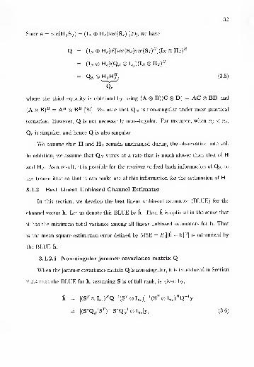
3. 1.2.1 Non-singular jammer covariance matrix Q

When the jammer covariance matrix Q is non-singular, it is introduced in Section

2.2.4 that the BLUE for h, assuming S is of full rank, is given by,

h = [(Sr

<g> I„r )

HQ_1

(ST

<g> Inr )]

_1(Sr

<g> I7lJ/fQ

_1y

= [(S*Q^1 St)

- 1S*Q^1 0lnr ]y, (3.6)

33

where we have used the fact (A ® B)-1 = A -1

(g> B _1[29] to obtain the second

equality. We also note that if e is a Gaussian random vector, then h given above

is also the maximum likelihood estimator (MLE), introduced in Section 2.2.5 from

Chapter 2, for h. Writing (3.6) back into matrix form, we have

H - YQ^S^SQ^S*)- 1. (3.7)

Moreover, the MSE of the BLUE is given by

MSE = £[||h-h|| 2

]

= tr[(Sr ®Inr )

//Q- 1(S

r<g)I„

r)]-

1

= tr[(ST

<g> Inr )

H(Q

N

® Qr)-1(ST ® UJ]-

1

= tr[(S*Q^1 ®I„r

Q- 1)(S

T ®I„r)]-

1

- tr[(S*Q^1 ST)®Q7 1 ]- 1

= tr[(S*Q^1 Sr)- 1

]tr(Q r ). (3.8)

The second equality is obtained from ||X||2 = tr{XHX}. The fourth and fifth equali-

ties are obtained by using (A®B)(C®D) = AC®BD and (A®B) _1 — A -1 ®B _1.

The last equality is due to tr(A ® B) = tr(A)tr(B) [29].

3. 1.2. 2 Singular jammer covariance matrix Q

In this section, we focus on the case of singular Q. First, write the spectral

decompositions of Qn and Q r ,respectively, in the following forms:

1

>•o

1 u"Qv — Uv U*

•

0 0 UX>N

= IEvAjvU"

LjV

Qr

r A r 0 u"Ur U r

0 0 u"U r

UrArUf, (3.9)

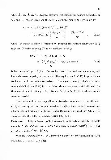
34

where AN and A r are the diagonal matrices that contain the positive eigenvalues of

Qw and Q r ,respectively. Then the spectral decomposition of Q is given [29] by

Q (U/v ® Ur )(Ajv ® A r )(Ujv U r )

H

(Uat ® U r )U

Ajv ® Ar 0 (Ujv ® U r )

H

0 0 \JH

(3.10)

where the second equality is obtained by grouping the positive eigenvalues of Q

together. Consider applying \JH

to the received vector y:

U"y = U ff(ST 0 I„

r)h + XJ

He

= \JH

(ST

(g) I„r )h with probability 1. (3-11)

' v

—

X

Indeed, since JV(Q) = 7£(U), U /7 e has both zero mean and zero covariance, and

hence the second equality above results. The requirement in (3.11) imposes a con-

straint on the linear estimation problem. If we neglect those y (which occur with

zero probability) that (3.11) is not satisfied, then a consistent model will result for

the constrained estimation problem. We use the triple (y, Xh, Q) to denote such a

consistent model.

The constrained estimation problem mentioned above can be conveniently stud-

ied by employing the theory of generalized inverses [31]. First, we have to make sure

a linear unbiased estimator for h exists under the constrained model (y, Xh, Q). To

do so, we need the following characterization [31, Ch. 6].

Definition 1. A linear function c^h is referred to as linearly unbiasedly estimable

under (y, Xh, Q) if there exists a vector a and scalar a such that E[&Hy + n] = c /7h

for all h such that \JHy = UHXh.

With this characterization, the follow result specifies the set of all linear unbiased

estimators of h under (y, Xh, Q).

35

Theorem 4. The function c77h is linearly unbiasedly estimable under (y, Xh, Q) if

and only if c € 7£(XH ). Moreover, if this condition is satisfied, the set of linear

unbiased estimators for c7/h is given by {a 7/h : a /7X = c

77}.

Proof. See the proofs of Theorems 6.4.1 and 6.4.2 in Campbell and Meyer [31].

Corollary 1. Suppose that the training symbol matrix S is of full column rank. Then

every Ay such that A(Sr ®I„r )= Intnr

is a linear unbiased estimator for the channel

vector h.

Proof. Since S is of full column rank, X = S 7<8)I„

ris of full row rank [29]. Let e*, for

% = 1,2,..., ntnr ,denote the elementary vectors of dimension n tnr . Then they are all

in TZ(XH ). Thus, efh, for i — 1,2, . .. ,n tnr ,are linearly unbiasedly estimable, and

the set of linear unbiased estimators for h is {Ay : AX = by Theorem 4.

Next, we turn to finding the BLUE for h with the assumption that S is of full

column rank. To do so, we need to introduce some generalized inverses of a matrix

[31]-

Definition 2. Moore-Penrose inverse and (l)-inverse:

(a) The Moore-Penrose inverse, At, of a matrix A is the unique matrix that satis-

fies:

(i) AAtA = A,

(ii) AtAAt = At,

(in) (AAt)H = AAt, and

(iv) (AtA)77 = AtA.

(b) A matrix A~ is called an (l)-inverse of A if A~ satisfies (i) above, i.e.,

AA“A = A. We denote the set of all (l)-inverses of A by A{1}. Obviously,

At e A{1}.

36

Hence, from Corollary 1, we need to consider all estimators of the form (Sr

<g>

I„r)-y. The following theorem provides a means to find the BLUE among these linear

unbiased estimators.

Theorem 5. Suppose that cHh is linearly unbiasedly estimable under (y, Xh, Q).

Let K, L, and M be three matrices that satisfy the following conditions:

(l) (Lvnr- XXf)D = 0,

(ii) QKX = 0,

(m) X^KQ = 0,

(iv) XHKX = 0,

(v) XWMX = D,

(vi) L G X{1}, and

(vii) XLQ = D,

where D = Q — QKQ. Then cHLy is the BLUE for cHh and the minimum variance

attained is given by cHMc.

Proof. See the proofs of Theorems 6. 4. 3-6. 4. 7 in Campbell and Meyer [31].

It turns out that the BLUE for H can be expressed in a form that is very similar

to (3.7). We will use Theorem 5 to demonstrate this.

Theorem 6. Suppose that the training symbol matrix S is of full column rank and

77(Sr)C 77(Qjv), where Qyv is the time correlation matrix of the jammer. Then the

BLUE for the channel matrix H is given by

H = YQtSH(SQtSH )t

(3.12)

with the minimum total variance (MSE)

MSE = MSQlS'y • ir(Qr ). (3.13)

37

Proof. Let

K = Qiv ® Qj - [QjvST(S*Q!vS

T)tS*Qjv ] ® Q|;

L = [(S*Q]vST)tS*Qj

v]®Inr

M = (S*QjvSr

)

t ® Q r .

Recall that Q = Qn <S> Q r and X = ST <g> I„r

. Hence, by employing the properties of

the Moore-Penrose inverse defined in Definition 2, it is not hard to see that

D = [Q iVQ!vSr(S*Q!vS

T)

tS*Q]vQ^®Qt

= [ST(S*QjvS

r)

t S*] <8> Qj

Indeed, we note that QyvQ/v is the projection operator onto 77(Qyv) [31]. Since

77(ST) Q 77(Q ^), we have QjvQjyST = ST . Hence the second equality above results.

We are going to show that this choice of K, L, and M satisfies the seven condi-

tions in Theorem 5.

(i) Note that 77(ST (S*QjvSr )t) C 77(Sr ). Hence 77(D) C 77(ST <g> I„

r ) [29].

Since I^nr — XXt is the projection operator onto the orthogonal complement

of 77(ST ® Inr ), (IiVnr- XXt)D = 0.

(ii) Like above, it is easy to work out that

QKX = [ST - Sr (S*QjvS

T)t(S*Q^ST)] ® Qr Q]:.

Hence, if (S*Q^ST)t(S’Q]vST)= I„

r ,then QKX = 0. From [31], what we

need is that S*QjvST

is of full rank (i.e., non-singular). To see that this is

indeed true, first we note that Qjy = UjvA- 1U^. Let N denote the rank of Q,v-

Since 77(ST)C 77(Qat) and ST is of full column rank, N > nt and S7 = UvS r

,

where S is a ntx N matrix with full column rank. Thus, S*Q^S r = s*A-N

lsT

is non-singular.

(iii) Similar to (ii).

38

(iv), (v) & (vii) Direct substitutions verify XHKX = 0, X;,MX = D, and X /7LQ =

D.

(vi) Indeed, XLX = [ST(S*Qjv S

r)

t (S*Q!vST

)] ® I„r= ST 0 I„

r= X, where the

second equality is due to the fact that S*QjvS7

is non-singular.

By Theorem 5, for i = 1,2,..., n tnr , efLy is the BLUE for efh with variance

efMe,. Eqns. (3.12) and (3.13) are simply compact ways to express these results.

To obtain (3.13), we have used the fact that tr(A <g> B) = tr(A) • tr(B) when A and

B are both square matrices [29].

3.2 Channel Estimation with Bayesian Estimator

3.2.1 System Model

We consider a transmitter-receiver pair with n ttransmit antennas and nr receive

antennas over a frequency flat fading channel in the presence of colored Gaussian

interference. We assume that the colored interference is composed of the thermal

noise and jamming signals transmitted by multiple jammers. The jth interferer has

rij transmit antennas. We assume that the transmission from the transmitter to the

receiver is packetized. Each packet contains a training frame that is composed of a

set of known training sequences, each of which is sent out by a transmit antenna. In

matrix notation, the observed training symbols at the receiver for a packet are given

byM

Y = HS +^H iS i +W = HS + E, (3.14)

i=iv

V'

E

where where S is the ntx N transmitted training symbol matrix that is known to the

receiver, N is the number of training symbols, and S, is the rq x N jamming signal

matrix from the ith jammer. We assume that symbols in S, are idem ically distributed

zero-mean, circular-symmetric complex Gaussian random variables, correlated across

both space and time. We assume that the number of training symbols N is larger

39

than nt . The jamming signals of the jammers are independent on each other. In ad-

dition, the jamming processes are assumed to be wide-sense stationary. We assume

that the number of training symbols N is larger than nt

. The nr x n t matrix H and

nr x rii matrix Hj are the channel matrices from the transmitter and the zth jammer

to the receiver, respectively. We assume that the elements in H and Hsare inde-

pendent, identically distributed zero mean complex Gaussian random variables with

variance a2 and a2,respectively. In addition, W is an additive white Gaussian noise

(AWGN) matrix and the elements in W are assumed to be independent, zero-mean,

circular-symmetric, complex Gaussian random variables with variance a Finally,

H, Hi, . .. , Ha/, Si, ...

,Sm, and W are all independent of one another.

3.2.2 Bayesian Channel Estimator

Let y = vec(Y), h = vec(H), and e = vec(E), where wec(X) is the vector

obtained by stacking the columns of X on top of each other . Taking transpose and

then vectorizing on both sides of (3.14), we have [29]

y = (Sr ®I„

r)h + e, (3.15)

where <S>, (-)T

,and I„

rdenote the Kronecker product, transpose of a matrix and

nr x nr identity matrix, respectively. In (3.15), h is a channel vector with distribution

A/f(0, CH )where the covariance matrix CH = Ejhh 7

'] = a2Inrnt and e is a noise

vector with distribution A/”c (0, Q) where the covariance matrix Q = E[eeH ]. We

assume that e is independent of h. During the training period, the Bayesian estimator

of the channel vector h based on the received training block Y, introduced in Section

2.3, can be obtained as

h = |(S7 ' ® I„

r )"Q''(ST ® I,„) + C^l

]-‘(ST ® I„

T )

HQ- 1

y. (3.16)

40

We note that the noise vector

Me = nec(HjS;) + nec(W)

i=i

M= ^(SiT ®Hi)wec(I„,)+»ec(W). (3.17)

2=1

El4i«kj^lm

Let s\j be the jamming symbol transmitted by the kth antenna of the ith jammerat

at time j and

Rk,kti’ m)for k = l

for k ^ 1,

where Rk k (j, m) is the time correlation between the jamming symbols at times j and

m from the kth. antenna of the ith jammer and Rkl (j,m )is the spatial correlation

between the jamming symbol at time j from the /cth antenna and the jamming symbol

at time rn from the Ith antenna of the ith jammer. Then the Nnr x Nnr noise

correlation matrix is given by

M

Q - Ê[(S i

T ®H i)êc(In i)^c(InJ

i/(S l

T ®H,) /y

]

2=1"V-J

H I+£'[nec(W)nec(W)

J +

In (3.18), the Nnr x Nnr matrix J can be easily obtained as

(3,18)

Mj = E O,

2=1

M

E RiA°) • Ck=

1

E Ri,t(N -1)'I"Lfc=l

EfiE(iv-i)-i.:k=

1

E RlA0) • I.:

k=

1

5^(a.

? QSv ® ^r).

(3.19)

(3.20)

2=1

41

where

E *U°)k=

1

E %(*' -1)

E K,*(N ~ i)

fc=l

E 4*(o)

(3.21)

Lfc=l fc=l

and Rkk(m — n) = k (m, n) because of the wide-sense stationary assumption. The

derivation for J in (3.19) can be found in Section 3.4. Due to the i.i.d assumption we

made on the elements of the channel the space correlations between interference

symbols from different antennas play no role in the correlation matrix Q. As a result,

only time correlation terms remain in (3.19).

Thus the noise correlation matrix Q is given by

MQ = ® Inr )

+ °2J-Nn

i—\

M= E + °11n ) ® Inr (3.22)

i= 1

The second equality is obtained from (A®B) + (C<g>B) = (A + C)®B [29]. By using

the Kronecker product form of Q obtained in (3.22), the Bayesian channel estimator

in (3.16) can be reduced to

h = S*A^Sr + \lntaH

-1

S*A^ (3.23)

where

MAat -^ of + of,Ijv- (3.24)

2—1

In addition, we can write (3.23) back into matrix form as

H = YAZ'S*(SAZ1 SH +

v2

-1

(3.25)

42

Moreover the MSE of the Bayesian estimator for H, discussed in Section 2.3, is given

by

MSEW = tr[(ST

<g> InJ//Q

_1(Sr

<g> I„r )+ Cjj

1

]

-1

M= tr[(S

T®Inr)

H{'%2°iQN +Îiv)®Inr }

_1(S

r ®I„r )

i=

1

+ (°2Kn t ) *]

1

Mtr[{S*(â,2q“ + <7

2Iw)-'S

t ® I„r } + ® I.,}]"1

i= 1

M ' 1 _1

s,(£^Q&) +^W- i st + î„i=l

M

trcr^

= tr[{S-(£o?Q« + oil*)1 Sr + Înt }

x

]

i=l

= nr • tr S*A^ST + 4ln(

-1

(3.26)

where ()*, (-)H

,and tr(-) denote the complex-conjugate, complex-conjugate (Hermi-

tian) transpose and trace of a matrix, respectively. The third and fourth equalities

are obtained by using (A®B)(C®D) = AC®BD, (A®B) + (C®B) =(A+C)®B,

and (A <g> B)_1 = A -1 ® B _1

. The fifth equality is due to tr(A ® B) = tr(A)tr(B)

[29]-

We assume that the channel matrices H and Hj for i — 1, . ..

,

M are short-term

statistics that may change from packet to packet. On the other hand, the interference

correlation matrix Q varies at a rate that is much slower than that of the channel

matrices. As a result, it is possible for the receiver to estimate Q using a number

of previous packets and feed back relevant information to the transmitter so that it

can make use of this information to select the optimal training sequence set for the

estimation of H during the current packet.

43

3.3 Summary

We described a transmitter-receiver pair in MIMO system model over frequency

flat fading channel in the presence of colored interference. We developed the BLUE

for the MIMO channel and derived the MSE expressions of the BLUE when jammer

covariance matrices are non-singular and singular cases. In the Bayesian approach,

we considered the case where there are multiple interferers. We obtained the Bayesian

estimator and derived the MSE expression of the estimator. From the expression of

the MSE for both estimators, we note that the MSE of the channel estimator depends

on the choice of the training sequence set S. We will discuss how to optimize the

training sequences to minimize MSE of the channel estimator in the following chapter.

3.4 Derivation of the J Matrix

Let the rii x N jamming signal matrix S* and nr x n* channel matrix from the

jammer EU be

and

S,=

’1,1 °l,N

ni, 1 °ni,N

Hj =

/>*"1,1

hn r ,n i

We note from (3.17) that noise vector e is expressed by

Me =5>T

<g> Hi)vec(lni ) + wec(N).

»=

i

(3.27)

44

Let us just consider the first term in (3.27)and let e be

Me = y^(S t

r<S> H t )vec(InJ

i—

1

/ _ 2 „2 2 \

m

E*1,1 *2,1

’ ‘‘ 6

ni,l

® Hii= 1

V 4 ,N 4,N ••• 4itN_ /

vec(I„J

= EZ=1

Sl,lHi s2,l^j' ' ' Sn t

,lî

sj)7VHj s^Hi •

• • sl

n . NHi

yec(Ini )

ni-rii x 1

iV-nr XTij-rii

(3.28)

We can easily see that [uec(I„t )]

Tis

[r;ec(Int )]

r = [10 ••• 0010 ••• 0 0 0 1 0 ••• Q

V*

1 XTli-Tii

(3.29)

Therefore we can obtain (3.28) by simple matrix multiplication and (3.28) can be

rewritten by the following N nr x 1 vector e

45

M

Ei=i

4.14.1 + 4,iM)2 + 4,i-4,3 +

4.14.1 + 4,l4,2 + 4,l4,3 +

h L

t>ni,l

n2,rii

> nr x 1

4,l4r ,l + 4,l4r ,2 + 4,l4 r ,3+ • •

• + <,l< )ni ,

4,24,1 + 4,24,2 + 4,24,3 + • • • + snj,24,r»i

4,24,1 + 4,24,2 + 4,24,3 + • •• + 4i,24, Tii

4 )24r ,i + 4,24r ,2 + 4,24r ,3+ • •

• + 4,24,,^

> nr x 1

> iV • nr x 1

4,iv4,l + 4,jv4,2 + 4,iv4,3 + • •• + 4i ,7v4,n,

4,jv4,l + 4,jv4,2 + 4,1V 4,3 “I f sn i ,jv4,n <

4,iv4r ,l+ S2,Nhhr,2 + 4,jv4r,3 _l *" 4i,lV^

> nr x 1

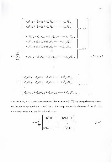
l

Let the N-nr xN-nr covariance matrix of e be K = J5[eeff

]- By using the assumption

on the jamming signal matrix and the i.i.d assumption on the elements of the Hj, the

covariance matrix K can be reduced to as

MK = E

1=1

K?(0)

K*(iV — 1)

K J (iV- 1)

K l

(0)

(3.30)

46

where r in K l(r) is the time difference between jamming symbols for r = 0, 1, 2,

••

,N—

1, K l

(r) is an nr x nr diagonal matrix and is given by

0

A:=l

(3.31)

0

where rij is the number of antennas at the zth interferer, Bl

k k (r) is the time correlation

between the jamming symbols from the A;th antenna of the zth jammer and of is the

variance of the channel from the jammer. All the space correlation terms are removed

due to the i.i.d assumption on elements of the channel from the jammer. Moreover,

(3.31)

can be further reduced to

(3.32)

Thus, the covariance matrix K is expressed by

E -1) i E *U(0) • In

E «U(o) E KAN -1)

M<g>I; (3.33)

i= 1

E KAN -!)

• •• E KAO)

Therefore we finally obtain J in (3.19).

47

Table 3-1: Matrix Notation

Aa

In

0

diag(xi, . .. ,xn )

Ar

A*

AH

tr(A)

rank(A)

A“A t

vec(A)

A® B71(A)

A7(A)

capital letters in boldface denote matrices

lowercase letters in boldface denote column vectors

n x n identity matrix

zero matrix

diagonal matrix with X\, ... ,xn as the diagonal elements

transpose of Acomplex conjugate of Acomplex conjugate transpose (Hermitian) of Atrace of Arank of A(l)-inverse of AMoore-Penrose inverse of Avector obtained by stacking columns of A on top of each other

Kronecker product of A and Brange of Anull space of A

CHAPTER 4

TRAINING SEQUENCE OPTIMIZATION

We note from Chapter 3 that the MSE of the channel estimator depends on

the choice of the training sequence set S. Hence, it is natural to ask whether there

is an optimal set of training sequences that gives the best estimation performance.

Moreover, it is conceivable that the optimal training sequence set will depend on the

characteristic of the interference at the receiver. In this chapter, we determine the

optimal training sequence set that can minimize the MSE of the channel estimator

under a total transmit power constraint.

4.1 Optimal Training Sequence Set with BLUE

We note from (3.8) and (3.13) in Chapter 3 that MSE of the BLUE channel

estimator depends on the choice of the training sequence set. In this section, we

determine optimal training sequence set when we employ BLUE channel estimator.

To have a meaningful formulation of the sequence optimization problem, we need to

consider the following two restrictions. First, we limit the maximum total transmit

power of transmit antenna array to P. Second, we assume that the time correlation

matrix, QN ,of the jammer is non-singular. In addition, we recall that ST has to be

of full column rank for H to be linearly unbiasedly estimable. The following theorem

provides a constructive method to obtain the optimal training sequence set under

these restrictions.

Theorem 7. Suppose that the time correlation matrix, Qv, of the jammer is non-

singular. Let V be an arbitrary ntx nt unitary matrix. Also let , . .

.

,

A^ be the

nt smallest eigenvalues of Q^v, and U^ is the N x n t matrix whose columns are the

eigenvectors of Qn corresponding to X[N\ . .

.

,

X^\ respectively. Then the training

48

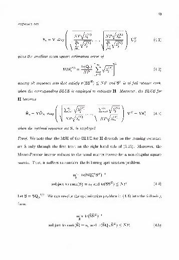
49

sequence set

V diag

VN

NPJ\\AN)

nt

i=iE A/Af

>

\

np/Npnt

3=

1

E x/Af)

U JV

7

gives the smallest mean square estimation error of

MSEfN) =tr{Q r )

NP

nt ,

—

I 2

(Y>

J=1

(4.1)

(4.2)

among all sequence sets that satisfy tr(SSH)< NP and S 1

is of full column rank,

when the corresponding BLUE is employed to estimate H. Moreover, the BLUE for

H becomes

H* = YU jv diag

/ X^nt X^n t

2-'j= i \Ar>\

u NP\Nr' ’\ NP\/A<r> 7

VH = YSl (4.3)

when the optimal sequence set S* is employed.

Proof. We note that the MSE of the BLUE for H depends on the training sequence

set S only through the first term on the right hand side of (3.13). Moreover, the

Moore-Penrose inverse reduces to the usual matrix inverse for a non-singular square

matrix. Thus, it suffices to consider the following optimization problem:

mm trfSQ^S*)" 1

subject to rank(S) = ntand tr(SS

H)< NP. (4.4)

Let S = SQjv1/2

. We can rewrite the optimization problem in (4.4) into the following

form:

min tr(SSH)

1

s

subject to rank(S) = ntand tr(SQArS ff

)< NP. (4.5)

50

Further, let pi , . ..

,

pnt be the (positive) eigenvalues of SS arranged in a descending

order and \[N\ . .

.

,

A be the eigenvalues of arranged in an ascending order. To

proceed, we need to make use of the following result, whose proof can be found, for

example, in [32, pp. 249].

Lemma 1. Suppose that X and Y are two Hermitian N x N matrices. Arrange the

eigenvalues Xi, ... ,x^ of X in a descending order and the eigenvalues yi, ... ,Pn of

Y in an ascending order. Then tr(XY) > YiLi xiVi-

Applying this lemma to the constraint in (4.5), we can bound

nt

tr(SQNSH

)= tv(QNS

HS) > JÂ^. (4.6)

i=i

Now, consider the following relaxed optimization problem:

minMl

Ei=i

Mi

, ...

subject to Y TiK < NP and pi > p2 > • • • > pnt > 0.

2—1(4.7)

If we can construct a matrix S such that the eigenvalues of SS 7/are exactly the

solution of the above relaxed optimization problem and that tr(SQ^S 77

} = Y hiK '

i=l

then this choice of S will be a solution of the original sequence optimization problem

in (4.5).

The relaxed optimization problem (4.7) can be solved by the standard Karush-

Kuhn-Tucker condition technique [33] since the cost function and the constraint are

both convex. The optimal solution is given by

NPn t

EJ=l

V

(N)A(A)

(4.8)

for 2 = 1,2,..., nt

. The derivation of this solution is given in Section 4.4. In addition,

the lower bound in (4.11) can be achieved by choosing S = Vdiag(-v/pY, . .. ,

w7t*]’)U]

where V and U/v are as specified in the statement of the theorem, and pi, . ..

,

p,ni

51

are given in (4.8). Hence, we get (4.1) by transforming back from the optimal choice

of S. In addition, the minimum value of MSE in (4.2) can be obtained by plugging

the optimal choice of p*, . ..

,

//*tin (4.8) back into the cost function in (4.7).

We note that not only does the choice of optimal sequence set minimize the

estimation error, but this choice also simplifies the implementation complexity of the

BLUE for H. It is easy to see from (4.3) that the complexity of the BLUE with the

optimal sequence set is 0(ntnrN). Finally, we point out that the training sequence

optimization problem is not very meaningful when QN is singular. In particular,

when rank(Qw )< N — n

t ,then according to the discussion in Section 3.1.2, one

can obtain zero MSE, for any arbitrarily small transmit power, by simply selecting

any full-rank S such that 77(ST)C J\f(QN ). When N — n t < rank(Qw) < N, one

can select N — rank(QAr) linearly independent sequences with arbitrarily small, but

non-zero, power from AZ’(Q^). Then the remaining power is allocated to sequences

that are found as in Theorem 7 restricting to Tl(QN ).

4.2 Optimal Training Sequence Set with Bayesian Estimator

Our goal is to minimize the MSE of the Bayesian estimator by selecting the

optimal training sequence set S with the total energy constraint tv(SSH

) < NP.

Therefore we can express the training optimization problem as follows:

nun tr[S*A^Sr + 4rl* t ]

-1(4-9)

subject to tv(SSH

) < NP,

Mwhere AN — ^ ofQV +Îw given in (3.24). Note that with the Bayesian approach,

i— 1

contrary to the classical general linear model, the training symbol matrix S need not

be of full rank to ensure the invertibility of [SÂ^1 ST + Mn,} [25].

Let S = SA^ '. We can rewrite the optimization problem in (4.9) into the following

52

form:

m_in trfSS^ + Înt ]

1(4.10)

subject to tr(SAjvS^) < NP.

Further, let /ii, . .. , //„ t

be the (positive) eigenvalues of SS arranged in a descending

order and A^, . .. ,A^ be the eigenvalues of arranged in an ascending order.

To proceed, we need to use Lemma 1 in Section 4.1. Applying this lemma to the

constraint in (4.10), we can bound

nt

trtSA^S") = tr(ANSHS) > J^to^- (4.11)

2=1

Now, consider the following relaxed optimization problem:

n t

min 2 {to + is) (4 - 12

)

A*1 v,/int i= \

subject to to^ ] < NP and £4 > • • • > /i„t> 0.

i= 1

This relaxed optimization problem can be solved by the standard Karush-Kuhn-

Tucker condition technique [33] since the cost function and the constraint are both

convex.

Let

n* - max k G {l,2,...,nt } : J \[N)

<

â2NP + J22=1

EVW\ <=i / J

(4.13)

We note that n* above is well defined and that the inequality that defines n* in (4.13)

holds for k = 1, . ..

,

n*, while it does not hold for k = n* + 1, . ..

,

n t . With this

53

definition, the optimal solution is given by

1

7

for k = 1, . .. ,n*

0 for k = n* + 1, . .. , rit-

We note that this solution has the standard water-filling [34] interpretation.

If we can construct a matrix S such that the eigenvalues of SSH are exactly the

solution of the above relaxed optimization problem and that tv(SANSH

) =i=

1

then this choice of S will be a solution of the original sequence optimization problem

in (4.10). Following the same procedure described in previous section, it is easy to

see that this can be done and the optimal training sequence set can then be obtained

as

where V is an arbitrary ntx nt unitary matrix and Un is the N x n t matrix whose

columns are the eigenvectors of AN corresponding to the nt smallest eigenvalues of

Atv- This optimal training sequence gives the smallest mean square estimation error

by plugging the optimal choice of /j,\, . .. ,

/r*(back into the cost function in (4.12).

We note that not only does the choice of optimal sequence set minimize the

estimation error, but this choice also simplifies the implementation complexity of the

channel estimator for H. It is easy to see that the Bayesian channel estimator in

(3.25) reduces to

(4.14)

of

(4.15)

H = YUN diag[w,, .

.

(4.16)

54

where

(4.17)

0 for k = n* + 1, . .. ,n t .

Thus the complexity of the Bayesian channel estimator with the optimal sequence set

reduces to 0(n tnr N).

We showed that the optimal training sequence sets can be obtained by solving two

optimization problems under the total transmit power constraint for both the BLUE

and Bayesian estimator cases. A simple physical interpretation of this solution is that

the optimal training sequence set put its power to where the effect of the jammer is

smallest, and hence the estimation error can be minimized. We note that the optimal

training sequence set is an orthogonal set if V is chosen to be an identity matrix.

However, the optimal training sequence set, in general, is not necessarily orthogonal.

For instance, it is possible to obtain a choice of V which spreads power evenly across

the transmit antennas with the use of non-orthogonal sequences. To do so, we need

to construct an unitary V to make the diagonal elements of

the same in both approaches. This is shown to be possible in Wong and Lok [35],

and such a V can be constructed using a simple iterative procedure.

In this section, the optimal solution for the training sequence optimization prob-

lem in the BLUE case in Section 4.1 is derived. To solve this optimization problem,

we use the standard Karush-Kuhn-Tucker condition technique [33]. We can easily

obtain the optimal solution for the Bayesian estimator case in the same way as the

following derivation.

4.3 Conclusion

(4.18)

4.4 Solution of the Optimization Problem

55

In this optimization problem, we only have inequality constraints. Thus opti-

mization problem can be expressed as

Nt

min £ (4.19)

Nt

subject to î(p) = ^ ^\\N ^ — NP < 0

2=1

= ~Hi < 0

93(H) = Hi ~ H2 < 0

9Nt+ i(h) HNt- 1— HNt

< 0.

Thus, we need to consider three conditions given by

8 > 0 (4.20)

Df(X) + 7T£>h(A) + 8

TDg{ A) = 0T

(4.21)

8Tg{ A) = 0, (4.22)

where 5 is the KKT multiplier vector and 7 is the Lagrange multiplier vector.

Because we do not have any equality constraints, the 7TDh{x) term in (4.21) is zero.

From (4.20) and (4.21), we have

5 > 0, 8T = [<5i, 82 ,

•

, Sfft+ i] (4.23)

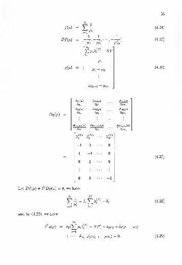
56

fit*)

Dm

git*)

Ei— 1

1

t*i

1

2 5

A*2

E - NP

~t*l

1*1 ~ t*2

t*Nt -l ~ t*Nt

Dg{n)

dg i(/x)

dm

dg2(v)

dm

9gi(/d

dmdg2{g)

dm

dgi(n)

d^Nt

dg2^)

dnNt

dgNt+ i(/A dgN

t+ i(m)

dm dmdgNf+iii1)

dHNt

A(AT)

1

-1 0 ••• 0

1 -1 ••• 0

0 1 0

0 0 -1

Let Df(/j;) + 6TDg(fi) = 0, we have

NtNt , Nt

Ei = *E A(N)

i= 1^ i=l

and by (4.22), we have

Nt

fiTg(t*) — $1 l*iî

N '

> — NP) — 52 t*\ +^3(^1—

1*2)

1=1

H h <^Vt+l(^JVt -l - UNt) — 0.

(4.24)

(4.25)

(4.26)

(4.27)

(4.28)

(4.29)

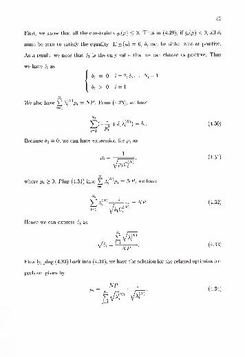
57

First, we know that all the constraints gi(g) < 0. Thus in (4.29), if gi(g) < 0, all Si

must be zero to satisfy the equality. If gt(g) = 0, Si can be either zero or positive.

As a result, we note that is the only value that we can choose as positive. Thus

we have Si as

jSi = 0

,i = 2

, 3, . .. , Nt + 1

|Si > 0

,* = 1

We also have A-^Vi = NP. From (4.28), we have2=1

Nt1

^(--+<S,A''' ))=i2 . (4.30)

i= 1^

Because S2 = 0, we can have expression for /q as

Ah =

where /q > 0. Plug (4.31) into ^ A^/q = -AAP, we have2=1

Nt

E a

2= 1

(iV) = NP.

S\C.(N)

Hence we can express as

(4.31)

(4.32)

(4.33)

Finally, plug (4.33) back into (4.31), we have the solution for the relaxed optimization

problem given by

NP 1

(4.34)

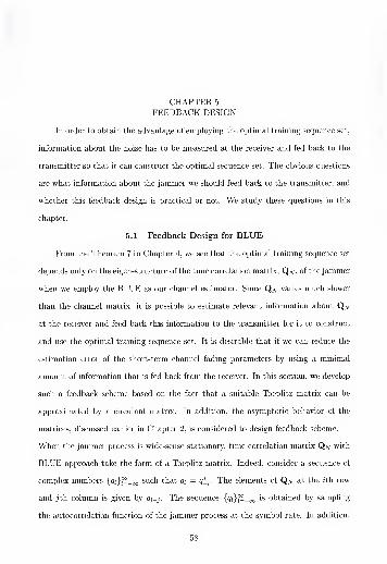
CHAPTER 5

FEEDBACK DESIGN

In order to obtain the advantage of employing the optimal training sequence set,

information about the noise has to be measured at the receiver and fed back to the

transmitter so that it can construct the optimal sequence set. The obvious questions

are what information about the jammer we should feed back to the transmitter, and

whether this feedback design is practical or not. We study these questions in this

chapter.

5.1 Feedback Design for BLUE

From the Theorem 7 in Chapter 4, we see that the optimal training sequence set

depends only on the eigen-structure of the time correlation matrix, Q^, of the jammer

when we employ the BLUE as our channel estimator. Since Q/v varies much slower

than the channel matrix, it is possible to estimate relevant information about Qat

at the receiver and feed back this information to the transmitter for it to construct

and use the optimal training sequence set. It is desirable that if we can reduce the

estimation error of the short-term channel fading parameters by using a minimal

amount of information that is fed back from the receiver. In this section, we develop

such a feedback scheme based on the fact that a suitable Toeplitz matrix can be

approximated by a circulant matrix. In addition, the asymptotic behavior of the

matrices, discussed earlier in Chapter 2, is considered to design feedback scheme.

When the jammer process is wide-sense stationary, time correlation matrix with

BLUE approach take the form of a Toeplitz matrix. Indeed, consider a sequence of

complex numbers {q,/}/T_ 00 such that qi = q*_v The elements of Q^v at the ith row

and j th column is given by qi_j. The sequence is obtained by sampling

the autocorrelation function of the jammer process at the symbol rate. In addition,

58

59

as we discussed in Section 2.4.3 in Chapter 2, if the sequence {<?;}^_00 is absolutely

summable that the Toeplitz matrix Q^v can be approximated by the circulant matrix

[27]

QN = FyyAjvF^, (5.1)

where F^ is the N x N discrete Fourier transform matrix, i.e.,the (k, l ) th element of

A is N x N diagonal matrix with S[

N\ . .

.

,

8^ as its diagonal12?r(fc — l)(f — 1)

-5= e J JV

elements.

Fyv is

A reasonable ways, as discussed in Section 2.4.3, to obtain SiN\ for l = 1, ... ,N

is

N

+ QN-k+ i)eJ2tt(A:-1)(/-1)

N

k=l

With this choice of S[N\ . .

.

,

6 it can be shown in Section 2.4.3 that Q.v

approaches as N approaches infinity. Moreover, if we arrange <Â\ . .

.

,

8^ in an

ascending order, we have

limN-*oo

VN > - V 1 = 0, (5.3)

for / = 1 ,...,n t. 8^ is the /th smallest eigenvalue among the set In

(5.3), \[N\ • •

•,X™

,defined in Chapter 4, are the nt smallest eigenvalues of Qat. In

summary, if we can estimate the autocorrelation function of the interference at the

receiver, we can obtain SjN

^ by (5.2). Then the n t smallest Sj^’s and the correspond-

ing indices are fed back to the transmitter. They correspond to the n t frequency

components of the noise that have the smallest power. At the transmitter, we can

replace A^, . ..

,

A^ and U/v, defined in Chapter 4, by the ntfrequency components

that have the smallest power. As a result, the receiver only need to feedback the

power values and indices of these n tfrequency components to the transmitter for the

construction of the approximate optimal training sequence set.

60

5.2 Feedback Design for Bayesian Estimator

In order to obtain the advantage of the optimal training sequence design, long-

term statistics of the interference correlation need to be estimated at the receiver

and fed back to the transmitter. We can conclude from Section 4.2 that the optimal

training sequence set depends on the channel gain variance a2 and the eigen-structure

of the matrix Ayv defined in (3.24) in Chapter 3. As a result, only these two long-term

statistics need to be estimated at the receiver. Since the interferer signals are wide-

sense stationary, AN takes the form of a Toeplitz matrix. Indeed, consider a sequence

of complex numbers such that a; = a*_tand the elements of A yv at the ith

row and jth column is given by a^j. The sequence {a;})T_O0 is obtained by sampling

the autocorrelation function of the interference at the symbol rate. In addition, as

we discussed in Section 2.4.3, if the sequence {a;}^T_ 00 is absolutely summable, then

it is shown in Gray [27] that the Toeplitz matrix A yv can be approximated by the

circulant matrix

An = FnAnFn, (5.4)

where is the NxN FFT matrix, i.e., the (k, /)th element of is -ê 3 n,

and A is a NxN diagonal matrix with <5^, . .. , 6

^

as its diagonal elements.

To obtain 5

j

N),for l = 1, . .

.

,

N, we use the same way in (5.2). With this choice

of \ . ..

,

it can be shown that Ayv approach An as N approach infinity [27].

Moreover if we arrange d[N\ . .

.

,

in an ascending order, we have

lim1

5

TV—>oo

(iV)

[l]A^l = 0

,(5.5)

for l = 1, . .

.

,nt ,and 5^ is the Ith smallest eigenvalue among the set {5^}^.

Now we turn to the estimation of cr2 and {cifcl^To

1- mentioned before, they

are both long-term statistics and hence should be estimated based on the observed

training frames of the previous K packets, where K is smaller than the number of

packets during which the long-term statistics remain the same. Toward this end,

61

let Sij(n) denote the (i,/)th element of the training matrix S(n) and yî{n) denote

the (z,/)th element of the observed training matrix Y(n) as defined in (3.14) for the

nth packet, respectively. Then it is not hard to see that for i — 1,2, ...,nr and

k = 0,1,. ..,N- 1,

(N - k)ak = EN-k

x E E y‘Ai)vij+kU) - °2NR‘n (k) (5.6)

j=n—K+ 1 1=1

where1

n N—k nt

K{k) =m E (5.7)

j=n-K+ 1 /=1 m=

1

In addition, let Ps(n) be the NxN projection matrix onto the subspace perpendicular

to the one spanned by the rows of the training matrix S (n) for the nth packet. Denote

the (i,/)th element of Y(n)Ps(n) by yî(n) and the (A:, Z)th element of Ps(n) by

pkti(n). Then it can be shown that for i = 1, 2, . .. ,nr ,

N-l

aoFn (0) + 2^ReM:(fc)] = £k—l

N

K Hi (5.8)

j=n—K+ 1 1=1

wheren N—k

KW = ~ E <5 - 9

)

j=n—K+l 1=1

We note that (5.6) for A; = 0, . ..

,

iV — 1 together with (5.8) provide us 2N

equations to solve for the 2N unknowns a2, do (both real-valued), and ak for k —

1, . ..

,

N — 1 (all complex-valued). Thus estimates of a2 and ak for k = 0, 1, . .

.

,

N — 1

can be obtained by solving this set of linear equations with the expectation terms

62

replaced by their usual estimates as follows:

nr n N

ao + a2Rs

n (0) = E ElVMi= 1 j=n—K+l 1=1

nr n N—k

ak + a2Rs

n {k ) - E E Ei= 1 j=n—K+l 1=1

^71 7* 71

°^v-i + cr2Rs

n{N —1) = ^Ê E 2/hiO')^,Jv(i)

i=l j=n—K+l

nr n N

a0 i?S(0) + 2£ R*M*(*)] = -Ê E EfcO')f-/ fcr

A=1

In above, the biased estimators

N-k

(5.10)

i= 1 j=n—K+ 1 i=l

AT

(V-fc

nr

~E E E yMvh+kU) - °2K(k)

i= 1 j=n—K+ 1 Z=1

for k = 0, 1, . ..

,

AT — 1, have been employed to approximate the corresponding expec-

tations on the right hand side of (5.6). We note that the use of these biased estimators

is similar to the use of biased autocorrelation function estimators in the Yule-Walker

method of estimating the power spectral density of an AR process [30].

In summary, we can use the solution of (5.10) to estimate the autocorrelation

function of the interference at the receiver and obtain estimates of the by

(5.2). Then the estimated value of <r2

,the n t smallest hE’s, and the corresponding

indices are fed back to the transmitter. At the transmitter, we can replace by

the columns of FN that are indexed by the feedback indices to construct the optimal

training sequence set for the current packet.

We note that the estimates of the ak s obtained by solving (5.10) do not guarantee

the resulting estimates of the 6k s and a2to be positive, although this is almost

always the case when N, K, and nr are sufficiently large. When the estimate of a2is

negative, we heuristically use the absolute value of the estimate instead. In addition,

63

we do not use those S^’s with negative estimates in finding the n t minimum values of

A^, . ..

,

A^ as described before.

5.3 Summary

In this chapter, we studied the way to feed back the required information from

the receiver so that we can obtain approximate optimal training sequence sets. This

feedback scheme is constitued based on the fact that a suitable Toeplitz matrix can

be approximated by a circulant matrix. In the following chapter, the performance

of the approximate optimal training sequence set obtained by the proposed feedback

scheme will be compared with different training sequence sets in terms of the MSE

of the channel estimator.

CHAPTER 6

NUMERICAL RESULTS

In this chapter, we present numerical results for the MSEs of the BLUE and

Bayesian channel estimator when three different training sequence sets are employed.

In addition, we introduce the asymptotic maximum MSE reduction ratio that can

tell us the maximum advantage we can obtain by employing the optimal training

sequence set over other choices of training sequences. Finally, conclusions will be

given based on these numerical results.

6.1 Asymptotic Estimation Performance Gain

It is illustrative as well as practical to develop a simple measure that can tell us

how much advantage we can obtain by employing the optimal training sequence set

over other choices of training sequences. For instance, if the receiver determines that

there is no much to be gain by using the optimal training sequences, it can inform the

transmitter to keep on using the current ones. To this end, we employ equal-power

orthogonal training sequences as our baseline for comparison, since these training

sequences are commonly [18-21] suggested when the noise is white.

6.1.1 BLUE

First, we want to obtain the worst-case MSE, MSE X ,when equal-power or-

thogonal training sequences are employed and the total transmit power is as least P.

It is not too hard to see that

max tr(SQ Ar

1 S//

)

1

SSH =iVPI<

nt

min Amin (SQ]v1 SH

)

SSH=NPl

max tr(SQiV

1 S H)

1 >ssh=npi

nt

min Amax (SQ^1 S //

)

SSW =JVPI

(JV)n

tANNP

„ 2 \WntAN-n t +l

' NP

(6 . 1)

64

65

where Am ;n (-) and Amax (-) are the minimum and maximum eigenvalues of a Hermitian

matrix, respectively, and A^,...,A^ are the eigenvalues of Qat arranged in an

ascending order. From Theorem 5, we can bound the worst-case MSE as

2 AN)niA

t ''N—nt+ l

NP< MSEffi

tr(Q r )

(N)

<n

tXNNP (

6 . 2)

On the other hand, Theorem 7 shows that when the optimal training sequence set is

employed,

n?AT MSEj") (S V^)NP ~

tr(Q r )NP ~ NP ' 1 ‘ ’

Combining (6.8) and (6.9), we can bound the ratio between the minimum MSE and

the worst-case MSE by

A^ MSE*** A^ }

\(N )

—MSE (7V) ~

An MDrjmax AN_nt+1

This MSE ratio gives the maximum possible relative reduction in the estimation error

that we can obtain by using the optimal sequence set under a specific jammer. To

obtain a simpler performance metric, we consider the asymptotic value of this MSE

ratio when N is very large.

Theorem 8. Suppose that the sampled autocorrelation sequence, {qn}<

%L- 00 > °f the

wide-sense stationary jammer process is absolutely summable. Let

OO

QM = W71—— OO

be the discrete-time Fourier transform o/{g„}^L_

^

lim A,-^ = minJV—xx) 0 <u)<2tt

. Then, for i — 1, 2, . .. ,nt ,

Q(uj)

lim A^ = max Q(co).JV-KX)

iV 1+1 0<ui<2n(6.5)

Moreover the asymptotic maximum MSE reduction ratio

„ main A Q{u)1 = lim —— = —

—

N~>oo MStiJV max Q(u)max 0<u<2n '

66

Proof. The results in (6.11) regarding the extremal eigenvalues of the sequence of

Toeplitz matrices {Q^} are proved in Grenander [36, Ch.5]. Applying (6.5) to (6.4),

we get (6.6).

6.1.2 Bayesian Estimatior

Similarly, we want to obtain the worst-case MSE, MSE X ,when equal-power

orthogonal training sequences are employed and the total transmit power is as least

P. It is not too hard to see that

max trssh=npi

SAt'S" +'-N a2^-nt

max tr

SSH=NP1SA^S"

min Amin(SAiV

1 SH) +

ssh=npi h

nt

~ N_P 1 , J_nt \(TV) ' cr

2AN

>nt

min Amax(SA iV

1 S^) + Arssh =jvpi

nt

NPnt

1

AN)'N-n t + l

+

y

(6.7)

where Am jn (-) and Amax (-) are the minimum and maximum eigenvalues of a Hermitian

matrix, respectively, and A^, . ..

,

A^ are the eigenvalues of AN arranged in an

ascending order. From (3.26), we can bound the worst-case MSE as

nrn t

NPnt

< MSEW <nrnt

AN)NPnt X'.

1 '/ a 2an

1

AN)(6 . 8

)

N—n$+l

On the other hand, from (4.15), when the optimal training sequence set is employed,

the minimum MSE can be bounded by

Tl'pTi^

NP 1

n* Ai

+ 1

<r2 AN )

< MSE^ <NP 1

A(TV) + 1 A

(TV)

T2 AN)An*

(6.9)

67

Combining (6.8) and (6.9), we can bound the ratio between the minimum MSE and

the worst-case MSE by

n*

n t

_1 I 1 n,

AN ) a2 NP

X(N) + a2

A(^V) NP

, AN)1 An« nt

<MSEf)

<n* Wl

MSEL^l ~ n t

+N— rif\-

1

1 nt

<72 NP

+. AN)1 A

i nt(6 . 10 )

AN) ^ a2 AN) NP/'n* /'n*

This MSE ratio gives the maximum possible relative reduction in the estimation error

that we can obtain by using the optimal sequence set under a specific set of interferers.

Here we obtain a simpler performance metric by considering the asymptotic value of

this MSE ratio when N is very large.

As described in the Theorem 8, we employ the following results regarding the

extremal eigenvalues of the sequence of Toeplitz matrices {A^r}. Suppose that the

sampled autocorrelation sequence, {an }^°-_ 0O ,of the wide-sense stationary interfer-

ence process is absolutely summable. Let

OO

A{u) = a"e~jUU1

77,=—OO

be the discrete-time Fourier transform of {an}£T_oo- Then, for i = 1, 2, . ..,nt ,

lim A<w

>

N—OO

lim AN—too

(N)

N—i+1

min A(u)0<w<2tt

max A(u>).0<w<2tr

(6 . 11

)

From (4.13) and (6.11), we see that lim n* = n t. Applying this and (6.11) to (6.10),

jV->oo

the asymptotic maximum MSE reduction ratio

r = limMSE{n)

N—>oo MSE^l

min A{uj)0<uK27r

max A(lu)0<ui<2tt

(6 . 12

)

6.2 Numerical Examples for BLUE

In this section, we introduce two jammer models to illustrate the potential ad-

vantage of employing the optimal training sequence set. The first model considers the

case when the jammer signal is a first-order auto-regressive (AR) random process. The

68

second model considers the case where the jammer is a co-channel interferer whose

signal structure is exactly the same as that of the desired signal. In each model, we

evaluate the MSEs of the channel estimators when following three different training

sequence sets are employed:

1. Hadamard sequence set, i.e.,first two rows of a Hadamard matrix are used as

the training sequences;

2. the optimal training sequence set described in Chapter 4. and

3. the approximate optimal training sequence set described in Chapter 5.

In each case, we assume that the desired user has two transmit antennas and two

receive antennas. Moreover, we assume that there is a single interferer. In each

example, we evaluate the MSEs, normalized by tr(Q r )(c.f. Eqn. (3.13)), of the BLUE

channel estimator when the three different training sequence sets are employed. In

each case, we consider different lengths of the training sequences (N — 16, 32, 64,

128, 256, 512, and 1024) and different signal-to-interference ratio (SIR = OdB, -15dB,

and -30dB).

6.2.1 AR(1) Jammer

We assume that the jammer is modeled by a first-order auto-regressive (AR)

process with AR parameter a that can be interpreted as the intensity of correlation

among the jammer symbols, i.e., with a larger value of a,the crosscorrelations among

jammer symbols are larger. The AR model is given [37] by

st = ast-i+ut , (6.13)

where u t is white Gaussian noise with zero mean, and variance It is easy to verify

that for this jammer,

1 + a2 — 2a cos uQ(v) = (6.14)

69

Hence, the asymptotic maximum MSE reduction ratio is given by

max Q(u)0<ui<2n

2

(6.15)

The MSEs of the BLUE channel estimator with the three different training se-

quence sets are shown and compared in Figs. 6-1 and 6-2 for the cases of a = 0.7

and 0.9, respectively. From these figures, we observe that there exist only minimal

differences between the MSEs of using the optimal training sequence set and approx-

imate optimal training sequence set. Obviously, this is a desirable result, because

it indicates that we can obtain almost same performance as that obtained by us-

ing the optimal training sequence set by feeding back much less information to the

transmitter. In general, we see that the optimal training sequence set significantly

outperforms the Hadamard sequence set for the two different values of a. The advan-

tage of using the optimal training sequence set increases as the correlation parameter

a increases. From (6.15), the asymptotic maximum MSE reduction ratio Y = — 15dB

and —25.5dB for the cases of a = 0.7 and 0.9, respectively. From Figs. 6-1 and 6-2,

we see that the MSE reduction ratios obtained by using the optimal sequence set

against the Hadamard sequence set are — 12dB and —22dB for the cases of a = 0.7

and 0.9, respectively. This means that the Hadamard sequence set gives MSEs that

are not much lower than the worst-case values.

Normalized

WISE

70

Figure 6-1: Comparison of MSEs obtained by using different training sequence sets.

AR-1 jammer with a = 0.7 and nt = nr = 2.

Normalized

MSE

71

N(Length of Training Sequence )


AR-1 jammer with a = 0.9 and n t = nr = 2.

72

6.2.2 Co-channel Interferer

We assume that the jammer is a co-channel interferer whose signal format is

exactly the same as the desired user signal. More precisely, let us assume that the

transmitted signal at the A:th transmit antenna of the jammer is given by

OO

sf(t) = - lT ~ T >’ <6 - 16>

/=— OO

(k)where b) is the sequence of data symbols that are assumed independent and iden-

tically distributed random variables with zero mean and unit variance, ip(t) is the

symbol waveform, T is the symbol interval, and r is the delay with respect to the

timing of the desired signal. Without loss of generality, we can assume that r G [0, T).

We also assume that \ip(t)\2dt = 1.

With the model described above, the elements of the jammer signal matrix Sj

in (3.1) and (3.14) are samples at the matched filter output at the receiver at time

iT. Specifically, the (k, i)th element of S j is given by

OO

[Sj]fc,<= ^2 b\k)

4>((i - l)T - t), (6.17)

/=— OO

where

/OO

x/j(t — s)ip*(s)ds (6.18)-OO

is the autocorrelation of the symbol waveform. Thus, we can express sampled auto-

correlation sequence as

qn =,m[^j]k,m+n}

oo

- Pj^2^((l-n)T-T)^(lT-T),/=— oo

(6.19)

73

and its discrete-time Fourier transform as

Q{u) = Pj

Pj_

JV

-0(nT + r)e Jl-JOJ7J

Tl=— 00

oo

I U) — 2tT A: \ .j(u-2nk)r

T (

—) e t

(6 . 20

)

where T(fl) = |^(fi)|2

,and 'l'(fl) is the Fourier transform of the symbol waveform

To illustrate how the use of the optimal training sequence set can benefit the

channel estimation process, let us consider the following two common symbol wave-

forms:

6.2.2. 1 Rectangular symbol waveform

In this case,

i’(t) =T, 0 < t < T

0, otherwise

and = <

t/T,

0 < t < T

2 - t/T,T <t <2T

0, otherwise.

From (6.20), we have

Q(uj)rr2 IT T

)

T

22T ,T

+ — (-T

T v T )cos a;].

(6 . 21

)

Hence, the asymptotic maximum MSE reduction ratio is

minQ(u;)

maxQ(w)

(¥)’ (6 .22

)

From (6.22), the use of the optimal training sequence provides no gain when the co-

channel interferer is symbol-synchronous to the desired user signal, i.e., r = 0. On

the other hand, when r = 0.5T, the asymptotic maximum MSE reduction ratio is 0.

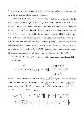
74

This means that we can almost completely eliminate the effect of the interferer by

using the set of long optimal training sequences.

In this section, we compare the MSEs of the BLUE channel estimator with the

three different training sequence sets in Figs. 6-3 and 6-4 for the cases of r = 0.3T

and 0.5T, respectively. Again, we observe that there exist only minimal differences

between the MSEs of using the optimal training sequence set and approximate optimal

training sequence set. From (6.22), the asymptotic maximum MSE reduction ratio

r = —8dB and —oodB for the cases of r = 0.3T and 0.5T, respectively. From Fig. 6-

3, we see that the MSE reduction ratio obtained by using the optimal sequence set

against the Hadamard sequence set is —4dB for the case of r = 0.3T. When r = 0.5T,

the results in Fig. 6-4 indicate that the MSE reduction ratio decreases as N increases.

These results are consistent with the asymptotic values predicted by (6.22).

6. 2. 2. 2 ISI-free symbol waveform with raised cosine spectrum [38]

In this case,

*(«)

T,

T2 1 1 + COS JL

20

0,

fr(l-ff)

T

o < \n\ <

ZLM < |fi| < e(M

M >

where 0 < 0 < 1 is the roll-off factor. Since J2kL- oo ^ ^k

)= T for all uj and ^(U)

is positive, it can be deduced from (6.20) that max Q{u) = Pj. To find min Q(cu),0<.u<2ir

because of symmetry of 'I'(U), it is enough to consider the interval uj G [7t(1 — @),n].

Over this interval, by (6.20), we have

Q{u>) =

+ 2 cos

P.i

(1 + cos

U1— 7r(l — 0) 1

2

+ 1 4- cos'to - 7r( i + py

1 [ 2/3 J [ w J

m2

(

2lT

)1 + cos

11r

-

H

V13l

1 + costo — 7f(l + 0)

\ T J L 2/3 jto "Co

Normalized

MSE

75


Co-channel interferer with rectangular waveform, r = 0.3T, and n t = nr = 2.

Normalized

MSE

76


Co-channel interferer with rectangular waveform, r = 0.5T, and nt = nr — 2.

77

0<w<27t

maximum MSE reduction ration is

Simple calculus reveals that min Q(u>) {l + cos (^fr)}- Thus, the asymptotic

(6.23)

From (6.23), the use of the optimal training sequence provides no gain when the co-

channel interferer is symbol-synchronous to the desired user signal, i.e., r = 0. On

the other hand, when r — 0.5T, the asymptotic maximum MSE reduction ratio is 0.

This means that we can almost completely eliminate the effect of the interferer by

using the set of long optimal training sequences.

In this section, we compare the MSEs of the BLUE channel estimator with the

three different training sequence sets in Figs. 6-5 and 6-6 for the cases of r = 0.3T

and 0.5T, respectively. Again, we observe that there exist only minimal differences


training sequence set. From (6.23), the asymptotic maximum MSE reduction ratio

T = —4.6dB and —oodB for the cases of r = 0.3T and 0.5T, respectively. From Fig. 6-

5, we see that the MSE reduction ratio obtained by using the optimal sequence set

against the Hadamard sequence set is —4dB for the case of r = 0.3T. When r = 0.5T,

the results in Fig. 6-6 indicate that the MSE reduction ratio decreases as N increases.

These results are consistent with the asymptotic values predicted by (6.23).

6.2.3 Average MSE with Hadamard Sequence Set

In this section, we evaluate the average MSE of the BLUE channel estimator

obtained by using the different rows Hadamard matrix as training sequences. Then

this result is compared with the MSE obtained by using optimal training sequence

set. The MSEs with the Hadamard training sequence set in Figs. 6-1 - 6-6 were

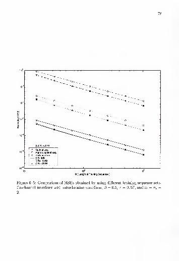
Normalized

MSE

78


Co-channel interferer with raised-cosine waveform, (3 = 0.5, r = 0.3T, and n t — nr =2 .

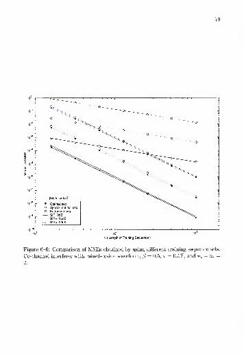
Normalized

MSE

79


Co-channel interferer with raised-cosine waveform, (3 — 0.5, r = 0.5T, and nt = nr —2 .

80

Figure 6-7: Comparison MSEs obtained by using optimal training sequence set with

average MSEs obtained by using all possible Hadamard training sequence set. AR(1)

jammer with a = 0.7 and n t = nr = 2.

obtained by arbitrary choosing sequences from the first two rows of the Hadamard

matrix. Because the MSE is dependent on the choice of the sequences, we average

the MSEs obtained by using all possible Hadamard sequence pairs. In Figs. 6-7 and

6-8, we see that the optimal training sequence set still gives significantly smaller

average MSE than using the rows of the Hadamard matrix as training sequences for

the two different values of a. In Fig. 6-9, MSEs are compared when the rectangular

waveform is considered as an interference signal. Like AR(1) model, we can still

obtain significant performance gain by using optimal training sequence set over the

Hadamard training sequence set.

Normalized

WISE

81


average MSEs obtained by using all possible Hadamard training sequence set. AR(1)

jammer with a = 0.9 and nt= nr = 2.

Normalized

MSE

82


average MSEs obtained by using all possible Hadamard training sequence set. Co-

channel interferer with rectangular waveform, r = 0.3T and n t = nr = 2.

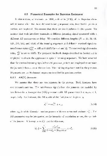
83

6.3 Numerical Examples for Bayesian Estimator

In this section, we evaluate the MSE, defined in (3.26), of the Bayesian chan-

nel estimator when the three different training sequence sets, described in previous

section, are employed. We assume that there are two interferers in the system. We

assume that each interferer transmits a different jamming signal generated with a

different AR parameters or delay. We consider different lengths (N = 16, 32, 64,

128, 256, 512, and 1024) of the training sequences and different received signal-to-

interference ratios = OdB and -20dB for i =1 and 2). The received signal-to-noise

ratio, is set to lOdB. The proposed feedback design described in Section 5.2 is

employed to obtain the approximate optimal training sequences. We have assumed

that the received training signals from 10 previous packets are employed to estimate

the jammer information at the receiver. The training sequences used in the previous

10 packets are the Hadamard sequences described in previous section.

6.3.1 AR(1) Jammer

We assume that there are two jammers in the system. Both jammers have

one transmit antenna. The interference signals from the jammers are modeled by

two first-order auto-regressive (AR) processes with AR parameters 0 < aq,Of2 < 1,

respectively. For instance, the AR model of the first jammer is given by

where is white Gaussian random process with zero mean and variance o2u X

. The

AR parameter can be interpreted as the intensity of correlation among the symbols

of the jammer. It is easy to verify that for this case,

(6.24)

(6.25)

84

Hence, the asymptotic maximum MSE reduction ratio is given by

1 am I 1

Z-/m=l o-g, l+qm ^(6.26)

y>2 d^l+% , i’2^m=l <72 i_Qm ^

.2

where Pm = -r^- is the transmit power of the mth jammer.

From the Figs. 6-10 - 6-11, we see that there exist only minimal differences


training sequence set. Obviously, this is a desirable result, because it indicates that we

can obtain almost same performance as that obtained by using the optimal training

sequence set by estimating the jammer information at the receiver and feeding back

only a small amount of information to the transmitter. In general, we see that the

optimal training sequence set significantly outperforms the Hadamard sequence set

in all the cases considered. The advantage of using the optimal training sequence

set increases as the correlation parameters cq’s increase. The asymptotic maximum

MSE reduction ratios for the cases considered above are shown in Table 6-1. For

comparison, the MSE reduction ratios obtained by using the optimal sequence set

against the Hadamard sequence set for N = 1024 are also included in Table 6-1.

We can deduce from the table that the Hadamard sequence set is rather inefficient.

In addition, much more reduction in the MSE can be obtained using the optimal

sequence set when both of the cq’s are close to 1.

6.3.2 Co-channel interferer

In this example, we assume that the interference is caused by two co-channel

interferes whose signal format is similar to that of the desired user. More precisely,

let us assume that the transmitted signal at the ith transmit antenna of the mth

interferer is given by

(6.27)

MSE

85


Two AR(1) interferers with a\ = 0.3 and a2 = 0.5.

MSE

86


Two AR(1) interferers with = 0.7 and a2 = 0.9.

87

where b is the sequence of data symbols, which are assumed to be i.i.d. binary

random variables with zero mean and unit variance, from the zth antenna of the mth

interferer, ip(t) is the symbol waveform, T is the symbol interval, and rm is the symbol

timing difference between the mth interferer and the desired signal. Without loss of

generality, we can assume that rm G [0,T). We also assume that \ip(t)\2dt = 1.

With the model described above, the elements of the interference signal matrix

Sm in (3.14) are samples at the matched filter output at the receiver at time kT.

Specifically, the (z, A;)th element of Sm is given by

4? = E hu]’&(* - or - rm ),

dm)

l=— oo

where

/OO

— s)ip*(s)ds

OO

(6.28)

(6.29)

is the autocorrelation of the symbol waveform. Thus, it is easy to see that the sampled

autocorrelation sequence

2 oo

a r=5Z °mPm W ~ n

)T ~ TmW(lT - t) + 02Jn , (6.30)

m= 1 l=- oo

and its discrete-time Fourier transform is given by

2

= Yl UmPr<

m— 1

E ^(nT + rm)e-*“

2 2 TD

_ ^2amPm

n=— oo

oo

771—1J»2 E *

cu — 27rk\ j(w-2*k)

Te T + (6.31)

where Pm is the transmit power from the mth interferer, T(f2) = |vh(0)| 2,and 'F(fi)

is the Fourier transform of the symbol waveform ip(

t

).

To illustrate how the use of the optimal training sequence set can benefit the

channel estimation process, let us consider the following two common symbol wave-

forms:

6.5.2. 1 Rectangular symbol waveform

In this case,

88

xl){t) =1/T, 0 <t<T

0, otherwise

and x/(t) = <

t/T,

0 < t < T

2 - t/T,T <t <2T

0, otherwise.

From (6.31), we have

am = $>;’

npm\

+ (i -r

^y + 2(!f)

(i -T

f) cos Id

m=

1

+ al (6.32)

Hence, the asymptotic maximum MSE reduction ratio is

v^2 cr^Pm2-jm=l o'?.

(22p - l)2+ l

V^2 °?n Prr, + 1

(6.33)

From (6.33), the use of the optimal training sequence provides no gain when

the co-channel interferers are symbol-synchronous to the desired user signal, i.e.

,

Ti— T2 — 0. On the other hand, when T\ = T2 = 0.5T, the asymptotic maximum

MSE reduction ratio attains its minimum value. This means that we can almost

completely eliminate the effect of the interferers by using the set of long optimal

training sequences.

Like before, we compare the MSEs of the Bayesian channel estimator with the

three different training sequence sets in Fig. 6-12 by considering the case in which

T\ = 0.3T and r2 = 0.5T. The other parameters are chosen as in the AR jammer

example before. Again from Fig. 6-12, we observe that there exist only minimal

differences between the MSEs of using the optimal training sequence set and ap-

proximate optimal training sequence set, and that the optimal training sequence set

significantly outperforms the Hadamard sequence set in all the cases considered. The

asymptotic maximum MSE reduction ratios for the cases considered above are shown

89

N

Figure 6-12: Comparison of MSEs obtained by using different training sequence

sets. Two co-channel interferes with rectangular waveforms and delays T\ = 0.3T,

r2 = 0.5T.

in Table 6-2. For comparison, the MSE reduction ratios obtained by using the opti-

mal sequence set against the Hadamard sequence set for N = 1024 are also included

in Table 6-2. We can deduce from the table that the Hadamard sequence set is rather

inefficient.

6. 5. 2. 2 ISI-free symbol waveform with raised cosine spectrum [38]

In this case,

T,

T(ft) = <

|{i + cos

[g(|ft|

0,

T

0 < |fi| <

eIM < |Q| <

\Q\ >

90

where 0 < /? < 1 is the roll-off factor. Since Yl'kL-oo ^ {~~y~ k

)= T for all uj and 'L(ff)

is positive, it can be deduced from (6.31) that max Aim) = cr‘i,Pm + <r2 To

find min A(co), because of symmetry of 'f'(fl), it is enough to consider the interval0<u<2n

uj e [7r(l — /3),7t]. Over this interval, by (6.31), we have

am = £2

alPrrm rn

+2 COS

m=

1

( 27TT„

(1 + cos

1

e i 4i

* i 3i - 2

+ 1 4- cosUJ — 7T (1 + /?)!

1 L 2p j L 2/? JJ

V T1 + COS

U) — 7r(l — /?)

~w 1 + COSuj - 7r(l + /3)

2/?+ °w-

(6.34)

Simple calculus reveals that min A(co) = Vi_, a£,Pm cos2 (^S3-) + oL

.

Thus, the0<w<27T

ism—

i

m \ l / m

asymptotic maximum MSE reduction ratio is

4- 12sm=l al ^ X

(6.35)

From (6.35), the use of the optimal training sequence provides no gain when

the co-channel interferers are symbol-synchronous to the desired user signal, i.e.,

7i = 72 = 0. On the other hand, when T\ = r2 = 0.5T, the asymptotic maximum

MSE reduction ratio attains its minimum value. This means that we can almost

completely eliminate the effect of the interferers by using the set of long optimal

training sequences.

Like before, we compare the MSEs of the Bayesian channel estimator with the

three different training sequence sets in Fig. 6-13 by considering the case in which

7"i= 0.3T and r2 = 0.5T. The roll-off factor of the ISI-free waveform is chosen to be

/3 — 0.5. The other parameters are chosen as in the AR jammer example before. The

conclusions from Fig. 6-13 are similar to those for the rectangular waveform.

MSE

91


Two co-channel interferers with ISI-free waveform waveforms and delays T\ = 0.3T,

r2 = 0.5T.

92

6.3.3 Bit Error Rate Performance

In this section, we evaluate the bit error rate (BER) performance by computer

simulation when the Bayesian channel estimator and the three different training se-

quence sets are employed. We assume that there are two transmit antennas and four

receive antennas. We also assume that there are two interferers in the system. Each

having one transmit antenna. Interferers are modeled by two AR(1) processes with

AR parameters aÔ.7 and a2=0.9, respectively. The training sequence length N is

64 and signal-to-interference ratios are OdB and lOdB. We consider different values

of signal-to-noise ratios from OdB to 40dB. In this simulation, we employ Alamouti’s

space-time block code [8]. The goal of this simulation is to examine the relationship

between the channel estimation performance obtained by using different training se-

quence sets and the corresponding BER performance.

Figs. 6-14 and 6-15 are the simulation results of the BER performance obtained

by using different training sequence sets. From these figures, we observe that we

can reduce BER significantly by using optimal training sequence sets against the

Hadamard training sequence set. Moreover, we see that there exist only minimal

differences between the BERs of using the optimal training sequence set and approx-

imate optimal training sequence set obtained by proposed feedback scheme. This

indicates that we can obtain almost same BER performance as that obtained by us-

ing the optimal training sequence set by feeding back much less information to the

transmitter.

6.4 Conclusion

Numerical results showed that the MSEs of the BLUE and Bayesian channel

estimator can be reduced significantly by using the optimized training sequence set

over the Hadamard training sequence set that is usually used. In addition, we ob-

served that we can obtain almost same performance by using the approximate optimal

training sequence set obtained by the proposed feedback scheme.

BER

93

Figure 6-14: Comparison of BERs obtained by using different training sequence sets.

Two AR(1) interferers with au = 0.7 and a2 = 0.9.

BER

94

Figure 6 -15: Comparison of BERs obtained by using different training sequence sets.

Two AR(1) interferers with a,\ = 0.7 and 0:2 = 0.9.

95

Table 6-1: Comparison of asymptotic maximum MSE reduction ratio and MSE ratio

between using optimal and Hadamard sequences in the case of AR jammers.

ot\ = 0.3, Qi2 = 0.5

SIR Asymp. max. MSE reduct, ratioMSE with optimal seqs. ^ Ar _ ino^MSE with Hadamard seqs. '

OdB—20dB

—7.08dB—7.46dB

—4.81dB—3.37dB

a i— 0.7, a2 = 0.9

SIR Asymp. max. MSE reduct, ratioMSE with optimal seqs. , AT _ 1AO/1 ^

MSE with Hadamard seqs. '

OdB—20dB

— 18.77dB

—20.30dB

— 15.56dB

— 10.05dB

Table 6-2: Comparison of asymptotic maximum MSE reduction ratio and MSE ratio

between using optimal and Hadamard sequences in the case of co-channel interferers.

Rectangular waveform T\ = 0.3T, t2 — 0.5T

SIR Asymp. max. MSE reduct, ratioMSE with optimal seqs. ^r _i nn^MSE with Hadamard seqs. '

OdB—20dB

—9.07dB— 10.94dB

—6.55dB—7.08dB

ISI-free waveform T\ = 0.3T, r2 = 0.5T

SIR Asymp. max. MSE reduct, ratioMSE with optimal seqs. , AT _ in0 /i\

MSE with Hadamard seqs. ^

OdB—20dB

—6.73dB—7.62dB

—4.54dB—4.34dB

CHAPTER 7

CONCLUSION AND FUTURE WORK

7.1 Conclusion

In this work, we addressed the problems of channel estimation and optimal train-

ing sequence design for multiple-input and multiple-output (MIMO) systems over flat

fading channels in the presence of colored interference. We considered two different

system models for which we applied two different channel estimators. The BLUE

channel estimator was considered for the case where there is single interferer with the

deterministic channel assumption. The Bayesian channel estimator was considered

for the case where there are multiple interferers. In the Bayesian approach, known

channel parameters that need to be estimated were assumed to be random with prior

PDF. This consititues the major difference between the two cases considered. We

showed that the MSEs of the considered channel estimators depend on the choice of

the training sequence set. Based on this observation, we addressed the problem of

optimal training sequence set design and obtained the optimal training sequence set

under a total transmission power constraint. In order to obtain the advantage of the

optimal training sequence design, we developed an information feedback scheme that

required a minimal amount of information from the receiver to approximately con-

struct the optimal training sequence set. Moreover, to obtain a simpler performance

metric, we introduced the asymptotic maximum MSE reduction ratio that could tell

us the maximum possible relative reduction in the estimation error that we could

obtain by using the optimal training sequence set under specific jammer models.

Numerical results showed that the MSEs of the channel estimators for both BLUE

and Bayesian estimator can be reduced significantly by using the optimal training

sequence sets, proposed in Chapter 4, over the Hadamard training sequence sets. In

96

97

addition, we verified from the numerical results that the approximate optimal train-

ing sequence sets, obtained by the proposed feed back scheme in Chapter 5, gave

estimation performance comparable to the optimal training sequence sets by utilizing

minimal information from the receiver.

7.2 Future Work

As discussed in Chapter 1, there have been two major approaches to design

optimal training sequence. One approach [9-13], [18], [21] is to determine the training

sequence that minimizes the MSE of the channel estimator. The other approach [14],

[20], [23] is to use information theoretic approach that uses lower bound of the channel

capacity. Frequency-selective fading channels have been considered in Vikalo et al.

[14], Fragouli et al. [21], Ma et al. [23] and all of these works use the information

theoretic approach to obtain optimal training sequences that can maximize some lower

bounds on the channel capacity. Most of these works have considered the presence of

only white noise. Not much work has been done to design optimal training sequence

in the presence of colored interference over frequency-selective fading channels.

In this dissertation, we have discussed the channel estimation and optimal train-

ing sequence design problems in the presence of colored noise over frequency flat

fading channels. Therefore, it is natural to extend this work to design optimal train-

ing sequence in the presence of colored interferece over frequency-selective fading

channels in MIMO systems.

Problem Approach

Let us consider the Bayesian channel estimator approach for the single interferer

case for simplicity. Multiple interferer case can be easily extended from the single

interferer case. The system model is given by

Y = SH + SjHj +W = SH + E, (7.1)

E

98

where the N x n tL training symbol matrix S is defined as

S = [S, S2... S„J, (7.2)

and L is the delay spread of the channel in symbol period, the N x L matrix S; is

given by

Si{0) 0 ••• 0

s*(l) Si(0) ••• 0

S> =Si(L — 1

) Si(L- 2) 3i(0)

(7.3)

Si(N-l) Si{N- 2) ••• Si(N-L)

for i = 1, 2, . ..

,

nt ,and the n tL x nr channel matrix H is given as

H =

/ipi • • • hi )7ir

hnt, i‘

‘' hnt 'Ur

(7.4)

with the Lx 1 vector = [hij{0) hitj( 1)

• • • hij(L —1)]

Tfor i = 1,2 , . .

.,n

tand

j = 1, 2, . ..

,

nr . E is the N x nr interference matrix that is composed of the thermal

noise and jamming signals from the jammer.

The Bayesian estimator, defined in (3.16), of the channel vector is obtained as

h = [(I„r ® S)

//Q- 1(Inr ® S) + Cj

/

1

]

_1(I„

r ® S)HQ~ 1

y, (7.5)

where the channel covariance matrix Ch = o2lnrnt . In addition, the MSE of the

Bayesian channel estimator, defined in (3.26), given by

MSE = tr[(Inr ®S)"Q-1(I„, aSJ + Cjj

1 ]- 1(7.6)

99

The objective is to find the training sequence set S in (7.2), which has block Toeplitz

structure as we note from (7.3), that can minimize the MSE of the Bayesian channel

estimator. Because of the structure constraint, it is not easy to find optimal se-

quences that satisfy the structure constraint. Thus, we may need to find sub-optimal

sequences instead. In addition, approximating the block Toeplitz matrix S could be

another way to tackle this problem.

REFERENCES

[1] G. J. Foschini, “Layered space-time architecture for wireless communication in

a fading environment when using multi-element antennas,” Bell Labs. Tech. J.,

vol 1, no. 2, pp. 41-59, 1996.

[2] I. E. Telatar, “Capacity of multi-antenna Gaussian channels,” Europ. Trans.

Telecommun., vol. 10, pp. 585-595, Nov. 1999.

[3] D. Gesbert, M. Shah, D. Sliiu, P. J. Smith, and A. Naguib, “An overview of

MIMO space-time coded wireless systems,” IEEE Journal on Selected Areas in

Communications, vo21. no. 3, pp. 281-302, Apr. 2003.

[4] V. Tarokh, N. Seshadri, and A. R. Calderbank, “Space-time codes for high data

rate wireless communication: performance criterion and code construction,”

IEEE Trans. Inform. Theory, vol. 44, pp. 744-765, Mar. 1998.

[5] V. Tarokh, H. Jafarkhani, and A. R. Calderbank, “Space-time block coding for

wireless communications: performance results,” IEEE J. Sel. Areas Commun.,

vol. 17, pp. 452-460, Mar. 1999.

[6] B. M. Hochwald and T. L. Marzetta, “Unitary space-time modulation for

multiple-antenna communication in Rayleigh flat fading,” IEEE Trans. Inform.

Theory, vol. 46, pp. 543-564, Mar. 2000.

[7] B. Hassibi and B. M. Hoclrwald, “High-rate codes that are linear in space and

time,” IEEE Trans. Inform. Theory, vol. 48, pp. 1804-1824, Jul. 2002.

[8] S. M. Alamouti, “A simple transimit diversity technique for wireless communi-

cations,” IEEE J. Sleet. Areas Commun., vol. 16, pp. 1451-1458, Oct. 1998.

[9] S. N. Crozier, D. D. Falconer, and S. A. Mahmoud, “Least sum of squared error

(LSSE) channel estimation,” IEE Proc. F., vol. 138, pp. 371-378, Aug 1991.

[10] G. Caire and U. Mitra, “Training sequence design for adaptive equalization of

multi-user systems,” Thirty-Second Asilomar Conference on Signals, Systems

and Computers, vol. 2, pp. 1479-1483, Nov. 1998.

[11] C. Tellambura, Y. J. Guo, and S. K. Barton, “Channel estimation using aperi-

odic binary sequences,” IEEE Commun. Lett., vol. 2, pp. 140-142, May 1998.

[12] C. Tellambura, M. G. Parker, Y. J. Guo, S. J. Shepherd, and S. K. Barton,

“Optimal sequences for channel estimation using discrete Fourier transform

technique,” IEEE Trans. Commun., vol. 47, pp. 230-238, Feb. 1999.

100

101

[13] W. Chen and U. Mitra, “Training sequence optimization: comparison and an

alternative criterion,” IEEE Trans. Commun ., vol. 48, pp. 1987-1991, Dec.

2000 .

[14] H. Vikalo, B. Hassibi, B. Hochwald, and T. Kailath, “Optimal training for

frequency-selective fading channels,” in Proc. Int. Conf. Acoust, Speech, Signal

Process., vol. 4, pp. 2105-2108, Salt Lake City, UT, May 7-11, 2001.

[15] W. H. Mow, Sequence design for spread spectrum, The Chinese University Press,

Hong Kong, 1995.

[16] W. H. Mow, “A new unified construction of perfect root-of-unity sequences,

” IEEE Fourth International Symposium on Spread Spectrum Techniques and

Applications (ISSSTA’96), vol. 3, pp. 955-959, Sep. 1996.

[17] D. C. Chu, “Polyphase codes with good periodic correlation properties,” IEEETrans. Inform. Theory, vol. IT-18, pp. 531-532, July 1972.

[18] T. L. Marzetta, “BLAST training: estimating channel characteristics for high

capacity space-time wireless,” 31th Annual Allerton Conference on Communi-

cation, Control, and Computing, Monticello, IL, Sep. 22-24, 1999.

[19] A. F. Naguib, V. Tarokh, N. Seshadri, and A. R. Calderbank, “Space-time

coding modem for high data rate wireless communications,” IEEE J. Select.

Areas Commun., vol. 16, pp. 1459-1478, Oct. 1998.

[20] B. Hassibi and B. M. Hochwald, “How much training is needed in multiple-

antenna wireless links?,” IEEE Trans. Inform. Theory, Aug. 2000. Submitted

for publication.

[21] C. Fragouli, N. Al-Dhahir, and W. Turin, “Training-based channel estimation

for multiple-antenna broadband transmissions,” IEEE Trans. Wireless Com-

mun., vol. 2, pp. 384-391, Mar. 2003.

[22] B. Park and T. F. Wong, “Training sequence optimization in MIMO systems

with colored noise,” in Proc. IEEE MILCOM ’03, Boston, MA, Oct. 2003.

[23] X. Ma, L. Yang, and G. B. Giannakis, “Optimal training for MIMO frequency-

selective fading channels,” IEEE Trans, on Wireless Commun., submitted for

publication, 2004

[24] E. G. Larsson and P. Stoica, Space-time block coding for wireless communica-

tions, Cambridge, UK: Cambridge University Press, 2003.

[25] S. M. Kay, Fundamental of statistical signal processing: Estimation theory, En-

glewood Cliffs, NJ: Prentice-Hall, 1993.

[26] J. M. Mendel, Lessons in estimation theory for signal processing, communica-

tions, and control, Englewood Cliffs, NJ: Prentice-Hall, 1995.

102

[27] R. M. Gray. (March/9/2004), Toeplitz and circulant matrices:

A review, Revised Aug 2002. [Online]. Available: http://www-

ee.stanford.edu/~gray/toeplitz.pdf

[28] Y. Song and S. D. Blostein, “Data detection in MIMO systems with co-channel

interference,” IEEE 56th Vehicular Technology Conference, vol. 1, pp. 3-7, Fall

2002 .

[29] R. A. Horn and C. R. Johnson, Topics in matrix analysis, Cambridge University

Press, 1991.

[30] S. M. Kay, Modern spectral estimation: Theory & application, Prentice-Hall,

New Jersey, 1988.

[31] S. L. Campbell and C. D. Meyer, Generalized inverses of linear transformations,

Pitman, London, 1979.

[32] A. W. Marshall and I. Olkin, Inequalities: Theory of majorization and its ap-

plications, Academic Press, New York, 1968.

[33] E. K. P. Chong and S. H. Zak, An introduction to optimization, Wiley, NewYork, 1996.

[34] T. M. Cover and J. A. Thomas, Elements of information theory, Wiley, NewYork, 1991.

[35] T. F. Wong and T. M. Lok, “Transmitter adaptation in multicode DS-CDMAsystems,” IEEE Journal on Selected Areas in Commun., vol. 19, pp. 69-82,

Jan. 2001.

[36] U. Grenander and G. Szego, Toeplitz forms and their applications,2nd ed.,

Chelsea, New York, 1984.

[37] S. Haykin, Adaptive filter theory,4th ed., Prentice-Hall, Upper Saddle River,

NJ, 2002.

[38] J. G. Proakis, Digital communications, 4th ed., McGraw Hill, New York, 2001.

BIOGRAPHICAL SKETCH

Beomjin Park was born in Seoul, Korea, in 1969. He received his bachelor’s

degree in electronic engineering from Hankuk Aviation University, Korea, in 1995

and the Master of Science degree in electrical engineering from the University of

Southern California in 1999. From 1995 to 1996, he was with Samsung Electronics

Co., LTD., Korea, as a product engineer. Since January 2000, he has been pursing his

Doctor of Philosophy degree in electrical and computer engineering at the University

of Florida in the area of wireless communications. His research interests include space-

time processing and channel estimation in multiple-input multiple-output (MIMO)

systems.

103

I certify that I have read this study and that in my opinion it conforms to

acceptable standards of scholarly presentation and is fully adequate, in scope and

quality, as a dissertation for the degree of Doctor of Philosophy.

Tan F. Wong, Chair

Assistant Professor of Electrical and Com-

puter Engineering




Yuguang “Michael” Fang,

Associate Professor of Electrical and Com-

puter Engineering




John M. Shea,

Assistant Professor of Electrical and Com-

puter Engineering




Louis N. Cattafesta III,

Associate Professor of Mechanical and Aerospace

Engineering

I certify that I have read this study and that in my opinion it conformsto acceptable standards of scholarly presentation and is fully adequate, in

scope and quality, as a dissertation for the degree of Doctor of Philosophy.

Assistant Professor of Electrical

and Computer Engineering

I certify that I have read this study and that in my opinion it conforms

to acceptable standards of scholarly presentation and is fully adequate, in

scope and quality, as a dissertation for the degree of Doctor of Philosot

Yug-tfang “Michael” Fang,

Associate Professor of Electrical




scope and quality, as a dissertation for the degree gif Doctor oN^hi osophy.

M. Shea,

Assistant Professor of Electrical




scope and quality, as a dissertation for the degree of Doctor of Philosophy.

Louis N. CattmestaAlI,

Associate Professor of Mechan-

ical and Aerospace Engineer-

ing

This dissertation was submitted to the Graduate Faculty of the College of En-

gineering and to the Graduate School and was accepted as partial fulfillment of the

requirements for the degree of Doctor of Philosophy.

May 2004 ) AjO^y^j-C —Pramod P. Khargonekar

Dean, College of Engineering

Kenneth J. Gerhardt

Interim Dean, Graduate School

Documents

Channel estimation in multiple-input multiple-output systems