Embed Size (px)
Citation preview

Dsp Implementation of channel
estimation algorithms for OFDM
systems
A Thesis submitted in partial fulfillment of the Requirements for the degree of
Master of Technology
In
Electronics and Communication Engineering
Specialization: Communication and networks
By
n. vijaya ratnam
Roll No. : 212EC5177
Department of Electronics and Communication Engineering
National Institute of Technology Rourkela
Rourkela, Odisha, 769 008, India
May 2014

Dsp Implementation of channel
estimation algorithms for OFDM
systems
A Thesis submitted in partial fulfillment of the Requirements for the degree of
Master of Technology
In
Electronics and Communication Engineering
Specialization: Communication and networks
By
N.VIJAYA RATNAM
Roll No. : 212EC5177
Under the Guidance of
Prof. Sarat K. Patra
Department of Electronics and Communication Engineering
National Institute of Technology Rourkela
Rourkela, Odisha, 769 008, India
May 2014

Dedicated to…
My late grandfather
My parents and my friends

i
DEPT. OF ELECTRONICS AND COMMUNICATION ENGINEERING NATIONAL INSTITUTE OF TECHNOLOGY, ROURKELA ROURKELA – 769008, ODISHA, INDIA
Certificate
This is to certify that the work in the thesis entitled DSP implementation of channel estimation
algorithms for OFDM communication systems by N.vijaya ratnam is a record of an original
research work carried out by her during 2013 - 2014 under my supervision and guidance in partial
fulfillment of the requirements for the award of the degree of Master of Technology in Electronics
and Communication Engineering (Communication and networks), National Institute of
Technology, Rourkela. Neither this thesis nor any part of it, to the best of my knowledge, has been
submitted for any degree or diploma elsewhere.
Place: NIT Rourkela Dr. Sarat Kumar Patra
Date: 23 May 2014 Professor

ii
DEPT. OF ELECTRONICS AND COMMUNICATION ENGINEERING NATIONAL INSTITUTE OF TECHNOLOGY, ROURKELA ROURKELA – 769008, ODISHA, INDIA
Declaration I certify that
a) The work contained in the thesis is original and has been done by myself under the general
supervision of my supervisor.
b) The work has not been submitted to any other Institute for any degree or diploma.
c) I have followed the guidelines provided by the Institute in writing the thesis.
d) Whenever I have used materials (data, theoretical analysis, and text) from other sources, I
have given due credit to them by citing them in the text of the thesis and giving their details
in the references.
e) Whenever I have quoted written materials from other sources, I have put them under
quotation marks and given due credit to the sources by citing them and giving required
details in the references.
N.vijaya ratnam
23st May 2014

i
ACKNOWLEDGEMENTS
It is my immense pleasure to avail this opportunity to express my gratitude, regards and
heartfelt respect to Prof. Sarat K. Patra, Department of Electronics and Communication Engineering, NIT
Rourkela for his endless and valuable guidance prior to, during and beyond the tenure of the project
work. His priceless advices have always lighted up my path whenever I have struck a dead end in my
work. It has been a rewarding experience working under his supervision as he has always delivered the
correct proportion of appreciation and criticism to help me excel in my field of research.
I would like to express my gratitude and respect to Prof. K. K. Mahapatra, Prof. S. Meher, Prof. P.
Singh, Prof. S. Ari, Prof. S. Maiti, Prof. A.K. Sahoo, Prof. S. Hiremath, Prof. A. Swain, Prof. S. K. Das and
Prof. S.K. Behera for their support, feedback and guidance throughout my M. Tech course duration. I
would also like to thank all the faculty and staff of ECE department, NIT Rourkela for their support and
help during the two years of my student life in the department.
I would like to make a special mention of the selfless support and guidance I received from my
senior Pallab Maji and Prashanth, department of Electronics and Communication Engineering, NIT
Rourkela during my project work. Also I would like to thank Saurabh Bansod and Baskar Jammu for
making my hours of work in the laboratory enjoyable with their endless companionship and help as well;
along with all other friends like Ragasudha,Karthik, Sandeep, Ravi, Saran Krishna, Venkatesh, Akhil,
Bhargav, Naresh, and many more who made my life in NIT Rourkela a memorable experience all
together.
Last but not the least; I would like to express my love, respect and gratitude to my parents,
friends and my late grandfather, who have always supported me in every decision I have made, guided

ii
me in every turn of my life, believed in me and my potential and without whom I would have never been
able to achieve whatsoever I could have till date.
Vijaya ratnam

iii
Dsp Implementation of channel
estimation algorithms for OFDM
systems
ABSTRACT
Channel estimation has a lengthy and big history in OFDM communication systems. For
this systems channel statistics need to track with simple techniques. Most of the OFDM channel
estimation techniques also useful to MIMO-OFDM systems. Efficiency high data rate and
performance of the wireless systems depends on estimation techniques. Generally present
estimation techniques can be categorized into two characters. The first type is based on the pilot
(known) data. Depending on pilot insertion divided into three type’s Block-Type, Comb-Type
Lattice –Type. Blind channel estimation techniques not require the pilot data, it requires previous
channel estimated information. I.e. Selected know data portion to be enforced for the channel
estimation. In this thesis, only the non-blind channel estimation techniques and stochastic gradient
algorithms will be analyzed and estimated using Simulink. By increasing pilot density efficiently,
we will track the channel variations, but it reduces the spectral efficiency. In wireless
communication systems receiver design is an integral part in that channel estimation also plays a
significant part. In general wireless communication systems know information is inserted at the
sender and this know information is recovered at the receiver by using the different channel
estimation techniques. In some cases it is possible to recover the transmitted information at the
receiver by using differential modulation techniques and channel estimation is not necessitated in
this Case but low data rate and wastage of SNR. In some other cases, the base station will complete

iv
the estimation part and sends a pre-distorted signal but it makes system degradation. Pilot insertion
is one of the main problem to estimate the channel on the receiver. Second one is tracking the
channel with limited pilot data and estimation with less complexity. OFDM systems
implementation and real-time estimation implementation using the Simulink is a challenging job.
The channel estimation based on the block - type, comb-type and lattice-type structure is
studied. The Block type pilot structure is performed on every block of OFDM symbols and the
Comb type pilot arrangement is performed on every OFDM symbol. Which are inserted particular
data intervals. Comb-type and block type spectrums are verified and the bit error rate is compared.
The objective of this thesis is to implementation channel estimation algorithm OFDM system
implementation of the C6713 Digital Signal Processor (DSP) of Texas Instruments (TI). First, the
basic channel LS and MMSE channel estimation techniques implemented and LMS, NLMS and
RLS were implemented and tested using Simulink Next this model is an implementation on DSP
C6713. Finally a comparison of the implemented estimator and compared BER values and mean
square error estimated in LMS NLMS and RLS algorithms performed.

v
CONTENTS
ACKNOWLEDGEMENTS ........................................................................................................................ i
ABSTRACT ................................................................................................................................................ iii
CONTENTS................................................................................................................................................. v
LIST OF FIGURES .................................................................................................................................. vii
NOMENCLATURE ................................................................................................................................ viii
ABBREVIATIONS .................................................................................................................................... ix
Chapter 1 ....................................................................................................................................................... 1
DESIGN AND IMPLEMENTATION OF OFDM SYSTEM ................................................................. 1
1.1 Introduction ........................................................................................................................................... 1
1.2 OFDM Implementation Using Simulink ............................................................................................. 2
1.2.1 System description ........................................................................................................................... 2
1.2.2 Simulink implementation ................................................................................................................. 4
1.3 Advantages and Disadvantages............................................................................................................ 6
1.4 Applications ........................................................................................................................................... 7
1.5 Motivation .............................................................................................................................................. 8
1.6 OFDM Channel Model ......................................................................................................................... 8
1.7 Channel Estimation Techniques .......................................................................................................... 9
1.8 Objective .............................................................................................................................................. 10
1.9 Thesis Organization ............................................................................................................................ 11
Chapter 2 ..................................................................................................................................................... 12
Channel Estimation in OFDM Systems .................................................................................................. 12
2.1 Pilot structures .................................................................................................................................... 12
2.2 Block-type ............................................................................................................................................ 12
2.2.1 Least Square Estimator .................................................................................................................. 14
2.2.2 Minimum Mean Square Estimation ............................................................................................... 15
2.3 Comb-Type .......................................................................................................................................... 16
2.3.1 LS Estimator with 1D interpolation ............................................................................................... 17
2.3.2 Second Order Interpolation ............................................................................................................ 19
2.3.3 FIR Interpolation (LPI) .................................................................................................................. 19
2.3.4 Splice Cubic Interpolation (SCI) .................................................................................................... 20
vi
2.3.5 Time Domain Interpolation (TDI) ................................................................................................. 20
2.4 Lattice-Type......................................................................................................................................... 21
CHAPTER 3 ............................................................................................................................................... 23
Adaptive Stochastic Gradient Algorithms Implementation .................................................................. 23
3.1 Introduction ......................................................................................................................................... 23
3.2 LMS Algorithm Implementation In Simulink .................................................................................. 24
3.2.1 Advantages ..................................................................................................................................... 26
3.2.2 Applications ................................................................................................................................... 26
3.3 NLMS Algorithm In Simulink ........................................................................................................... 27
3.4.1 Application ..................................................................................................................................... 28
3.3 RLS Algorithm Using Simulink ......................................................................................................... 28
Chapter 4 ..................................................................................................................................................... 31
Hardware Implementation of OFDM Channel Estimation Techniques Using C6713DSK ............... 31
4.1 Introduction ......................................................................................................................................... 31
4.2 DSK Support Tools ............................................................................................................................. 32
4.2.1 Required Software and Hardware .................................................................................................. 32
4.2.2 DSK Board ..................................................................................................................................... 32
4.4 TMS320C6713 Implementation ......................................................................................................... 33
4.5 OFDM Hardware Implementation Using c6713DSK ...................................................................... 34
4.6 Experimental setup and Simulink model .......................................................................................... 35
4.7 c6713DSK – Matlab Link Using the RTDX ...................................................................................... 36
4.7.1 Link uses RTDX ............................................................................................................................ 36
4.7.2 Using External Application ............................................................................................................ 37
4.8 Channel Estimation Techniques, Implementation in C6713dsk ..................................................... 39
Chapter 5 ..................................................................................................................................................... 42
Conclusion ................................................................................................................................................. 42
5.1 Conclusions .......................................................................................................................................... 42
5.2 Future work ......................................................................................................................................... 42
References .................................................................................................................................................. 43

vii
LIST OF FIGURES
Figure 1. 1 general OFDM block diagram ...................................................................................... 4
Figure 1. 2 Simulink OFDM model ................................................................................................ 5
Figure 1. 3 Simulink OFDM spectrum ........................................................................................... 5
Figure 1. 4 Simulink OFDM constellation ..................................................................................... 6
Figure 2. 1 block -type pilot structure ........................................................................................... 13
Figure 2. 2 block LS estimation .................................................................................................... 15
Figure 2. 3 comb-type pilot structure ............................................................................................ 17
Figure 2. 4 linear interpolation...................................................................................................... 18
Figure 2. 5 FIR Interpolation ........................................................................................................ 20
Figure 2. 6 Time domain interpolation ......................................................................................... 21
Figure 2. 7 Lattice-type ................................................................................................................. 22
Figure 3. 1Simulink LMS algorithm model .................................................................................. 25
Figure 3. 2 Simulink LMS channel estimation BER curve .......................................................... 26
Figure 3. 3 RLS performance curve .............................................................................................. 30
Figure 4. 1 TMS320C6713 board ................................................................................................. 33
Figure 4. 2 hardware setup ............................................................................................................ 36
Figure 4. 3 code generation part ................................................................................................... 38
Figure 4. 4 GPD output ................................................................................................................. 38
Figure 4. 5 setup diagram of interpolation channel estimation ..................................................... 39
Figure 4. 6 DSP bit error rate ........................................................................................................ 40
Figure 4. 7 LMS, NLMS, RLS, setup diagram ............................................................................. 41

viii
NOMENCLATURE
QH n-IFFT matrix
St Coherence time
f Doppler Doppler frequency
Kth N-subcarriers
g Channel impulse response
n AWGN channel noise
H Channel noise matrix
mmseH Minimum mean square estimation matrix
σmax Maximum delay
sf Coherence Band Width
W0 Weight vector
RY Auto covariance matrix
Rxy Cross covariance matrix
e(i) Error matrix

ix
ABBREVIATIONS
SISO-
OFDM
:
:
Single input single output –orthogonal frequency division
communication system
OFDM : Orthogonal frequency Division multiplexing
DAB : Digital Audio Broadcasting
IFFT : Inverse fast Fourier Transform
FFT
ISI
MIMO-
OFDM
WLAN
ADC
:
: : : : :
Fast Fourier Transform
Inter-symbol Interface
Multiple Input Multiple Output orthogonal Frequency Division
Multiplexing
Worldwide Interoperability For Microwave Access
Analog to Digital converter
DVB : Digital Video Broadcasting
DSP
BER
:
:
Digital Signal Processing
Bit Error Rate
DSK
GDP
CCS
TI
:
: : :
Digital Signal Processor Starter Kit
General Purpose Display
Code Composer Studio
Texas Instruments

x
SER
SNR
LMS
NLMS
RLS
GPD
RTDX
LS
MMSE
QAM
USB
TDI
SOI
LI
:
: : : : : : : : : : : : :
Symbol Error Rate
Signal to Noise Ratio
Least square algorithm
Normalized Least Square Algorithm
Recursive least square error
General purpose display
Real Time Data Exchange
Least squares
Minimum Mean Square Error
Quadrature Amplitude Modulation
Universal Serial Bus
Time Domain Interpolation
Second Order Interpolation
Liner Interpolation
1
Chapter 1
DESIGN AND IMPLEMENTATION OF
OFDM SYSTEM
1.1 Introduction
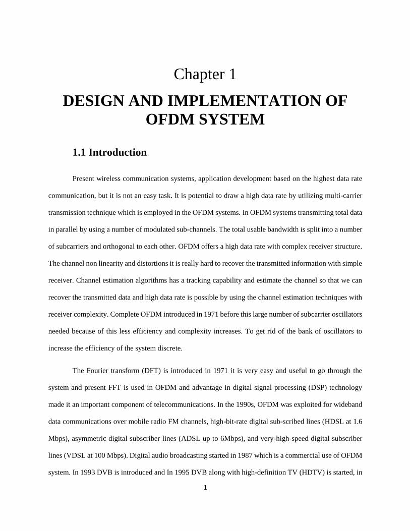
Present wireless communication systems, application development based on the highest data rate
communication, but it is not an easy task. It is potential to draw a high data rate by utilizing multi-carrier
transmission technique which is employed in the OFDM systems. In OFDM systems transmitting total data
in parallel by using a number of modulated sub-channels. The total usable bandwidth is split into a number
of subcarriers and orthogonal to each other. OFDM offers a high data rate with complex receiver structure.
The channel non linearity and distortions it is really hard to recover the transmitted information with simple
receiver. Channel estimation algorithms has a tracking capability and estimate the channel so that we can
recover the transmitted data and high data rate is possible by using the channel estimation techniques with
receiver complexity. Complete OFDM introduced in 1971 before this large number of subcarrier oscillators
needed because of this less efficiency and complexity increases. To get rid of the bank of oscillators to
increase the efficiency of the system discrete.
The Fourier transform (DFT) is introduced in 1971 it is very easy and useful to go through the
system and present FFT is used in OFDM and advantage in digital signal processing (DSP) technology
made it an important component of telecommunications. In the 1990s, OFDM was exploited for wideband
data communications over mobile radio FM channels, high-bit-rate digital sub-scribed lines (HDSL at 1.6
Mbps), asymmetric digital subscriber lines (ADSL up to 6Mbps), and very-high-speed digital subscriber
lines (VDSL at 100 Mbps). Digital audio broadcasting started in 1987 which is a commercial use of OFDM
system. In 1993 DVB is introduced and In 1995 DVB along with high-definition TV (HDTV) is started, in

2
1995 wireless local area network (WLAN) and Hiper LAN implementation started. OFDM has greater
importance because of this, it is anticipated to turn the technology of choice in most wireless links [11].
1.2 OFDM Implementation Using Simulink
1.2.1 System description
First input binary data are taken in and performed the coding this channel coded bits are
grouped together, and mapped to corresponding modulation constellation points. In this thesis 16-
QAM rectangular modulation is performed (QPSK, QAM etc.). At this period, data. In frequency
domain and the pilot are inserted here. A serial to parallel convertor is used. Data in frequency
domain convert into time domain by using IFFT data are grouped together again, as per the number
of required transmission subcarriers [5][9][8].
Let’s take the data sequence )}({ KX with a length of N by converting into the time domain
)}({ nx with the given following equation
x(n) = IFFT{X(K)} n = 0,1,2,…..N-1
=
1
0
)/2()(N
k
NknjekX (1.1)
After IFFT guard time need to insert to prevent the ISI, which is larger then the delay
spread. And add the cyclic prefix to the time domain signal .
The received signal is made by
)()()()( nwnhnxny (1.2)

3
Where w(n) is additive white Gaussian noise h(n) is a channel impulse response
Received signal is given by Y(K) = FFT(y(n)) where k = 0,1,2,3,…..N-1.
=
1
0
)/2()(/1N
n
NknjenyN (1.3)
H(k) = FFT(h(n))
W(n) = FFT(w(n))
Estimated pilot data channel HP(k) at pilot location and the estimated data after FFT is
given by
Xe = Y(k)/He(k) (1.4)
Cyclic prefix (CP) is inserted in each block of data in keeping with the system specification
and also the data multiplexed in a vary serial fashion At this time data are in time domain OFDM
modulated and ready to be shipped. After transmission of OFDM signal in wireless channel. Once
receive the signal at the recipient in time domain inserted CP is removed in receiver an FFT block
is used to demodulate the OFDM signal. At this level, i.e. In frequency domain channel estimation
is performed on complex received data pilots and complex data is dumped according to the
complex constellation diagram and coded information is decoded and recover the original binary
data. In this thesis we look at the precepts of an orthogonal division multiplexing (OFDM) systems.
Since our aim is to investigate channel estimation methods for OFDM systems using Simulink, it
is all important to acquire a firm understanding of OFDM systems in Simulink [1]. A pilot based
channel estimation general block diagram show in below fig. 1. 1.

4
Figure 1. 1 general OFDM block diagram
1.2.2 Simulink implementation
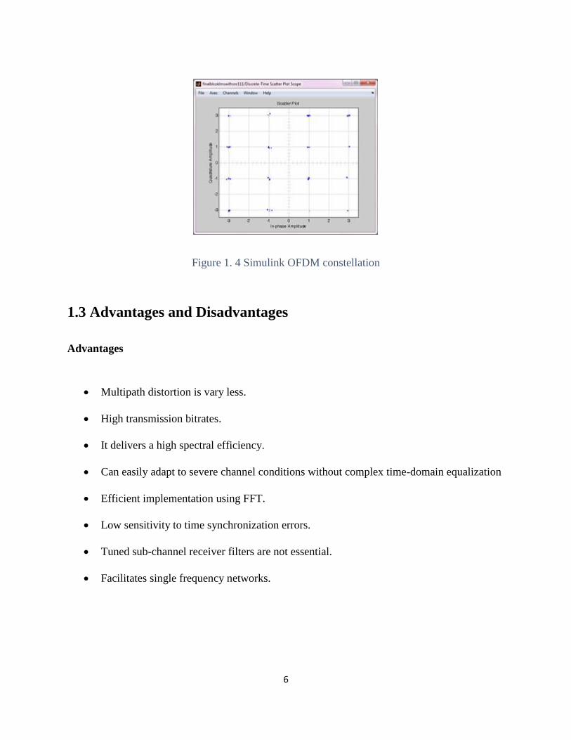
The Simulink model of OFDM system is described in the figure below figure 1.2 using 16-
QAM. The block included in this model are Bernoulli random binary integer generator, rectangular
QAM modulator, multiport selector, matrix consultation for selecting the pilots, zero padded IFFT,
Selector for adding a cyclic prefix, removing cyclic prefix, FFT, Remove zero padding, Remove
pilots for estimation, rectangular QAM demodulator, bit error rate block, RTDX (channel output).
Simulink OFDM spectrum and received constellation graphs show in figure 1.3 and figure 1.4.

5
Figure 1. 2 Simulink OFDM model
Figure 1. 3 Simulink OFDM spectrum
6
Figure 1. 4 Simulink OFDM constellation
1.3 Advantages and Disadvantages
Advantages
Multipath distortion is vary less.
High transmission bitrates.
It delivers a high spectral efficiency.
Can easily adapt to severe channel conditions without complex time-domain equalization
Efficient implementation using FFT.
Low sensitivity to time synchronization errors.
Tuned sub-channel receiver filters are not essential.
Facilitates single frequency networks.

7
Disadvantages
1. High synchronism accuracy
2. Complexity increase then the single carrier systems
3. Power and capacity loss due to guard interval
4. Considerable amount of bandwidth and power loss due to guard interval
5. Linear power amplifiers required
6. Multipath propagation must be avoided in other orthogonallity not be affected
7. High peak-to-average-power ratio (PAPR), requiring linear transmitter circuitry, which
suffers from poor power efficiency
8. Highly Sensitive to Doppler shift.
1.4 Applications
ADSL
DAB
HDTV
HIPERLAN/2
IEEE802.11g
IEEE802.11a/n
IEEE802.15.3a
IEEE802.16d/e
Broadband wireless access system IEEE802.16

8
Wireless ATM Transmission systems
International Mobile Telecommunications—Advanced Systems.
1.5 Motivation
To find the Performance of the any OFDM communication system. Perfect channel
knowledge is required. It is not possible in real time and we require to get the channel
characteristics and cognition of the channel by using channel estimation techniques depending on
the classifications mainly two types of channel estimation techniques using blind type and non-
blind type non –blind type channel estimation more efficient. Here we need to send the pilot
information through the channel which is known to the transmitter and receiver. Hardware
implementation in DSP processors more efficient than the other processors and also challenging
task in DSP processors. Simulink inspires you to try things out. You can easily build models from
a Simulink library and easy to edit the good examples. Simulink is a great tool to implement
practical and it will solve the real time problems. Simulink is used to carry out the dynamic
schemes. This is used to implement the models, easy to analysis and simulation. Simulink is used
in educational foundations, research, research labs, this is employed to reduce the real time
problems by using this SIMULINK library.
1.6 OFDM Channel Model
Consider an OFDM system with M subcarriers T
Nxxxx ]...................................,[ 110 this are
in frequency domain OFDM symbols. This symbol is converted into the time domain. By using the n-
IFFT [5].
by X = [X0,X1,……………..XN-1]T X = QHx where QH is a n-IFFT matrix.

9
)(/1 /2
,
Nmnj
nm eNQ for m,n = 0,1,……….N-1. (1.5)
And added cyclic prefix(CP) length assume L and at the receiver received OFDM symbols remove the
cyclic prefix at the receiver end is given by Y = [Y0,Y1,……………….YN-1]T
Y = HX + Z (1.6)
H is a channel matrix and Z is the time-domain noise vector
1.7 Channel Estimation Techniques
Of OFDM systems or MIMO OFDM system channel estimation is an integral part. This
communication system's efficiency depends on the different channel estimation techniques the
main thing is here to track the channel characteristics which are applied on the receiver side. Here
we are discussing only pilot added channel estimation techniques. Different type of channel
estimation techniques listed below.
Block-type
Least square estimation
Minimum mean square estimation
Modified mean square estimation
Estimation with decision feed back
Estimation with decision feed back
Comb-type
Least square estimation with linear interpolation

10
FIR interpolation
Cubic splice interpolation
Second order interpolation
Time domain interpolation
ML estimator
PCMB estimator
Another pilot – pilot based estimators
LMS
NLMS
RLS
KALMAN
Lattice filters
2D – dimensional estimators
1.8 Objective
1. The main object of the work is to reduce the complexity of estimation algorithms and
reduce the BER, increase the system efficiency without any complexity.
2. Study the channel estimation algorithms and understanding the different type of efficient
channel estimation techniques
11
3. Try to find the new channel estimation algorithm and implemented in OFDM system and
test the performance of the system and compare with the other channel estimation
techniques.
4. Implement this new technique in hardware using DSP and mixed processors and try to find
the efficiency and BER performance of the technique with real time.
1.9 Thesis Organization
The thesis has been organized into five chapters. This first chapter gives the introduction
about the OFDM, advantages and disadvantage of OFDM and application. Different types of
channel estimation techniques introduced in this first chapter and these are briefly summarized in
the next following chapters. The object of the work flow and motivation of the channel estimation
techniques is discussed in this chapter.
Chapter 2 The second chapter discuss the pilot based channel estimation techniques and hardware
implementation hardware implementation. Introduction to the RTDX and GDP, channel
estimation techniques, implemented in TMS320C6713 and compared with other techniques.
Chapter 3 The third chapter discuss about the gradient algorithms. LMS RLS AND NLSM
Its advantage and disadvantage and comparative study.
Chapter 4 The fourth chapter discuss about the channel estimation techniques, hardware
implementation. Results and discussions.
Chapter 5 The fifth chapter presents the conclusion to the complete work and talks about the scope of
future work to the research work that has been presented in the thesis.

12
Chapter 2
Channel Estimation in OFDM Systems
2.1 Pilot structures
Only restricted pilot data subcarriers are used for the primary channel estimation process.
There are two ways to insert the pilots, these are in time and frequency domain. The pilot spacing
is an important parameter generally this pilot are inserted in frequency domain and pilot spacing
depends on the coherence frequency of the channel. Power allocation and modulation of the pilot
data with regard to the factual data is an important parameter, if we increase pilot data power
channel estimation accuracy increase. Generally, data, symbol power and pilot data power are
equally considered. The performance of the system also depends on the pilot arrangement this pilot
arrangement should efficiently track the channel variations this is the one of the important topics.
Established along the pilot arrangement there are 3 forms of pilot arrangement are considered:
block type, comb type, and lattice type this 3 arrangements discussed in next sections the
estimation accuracy can be amended by increasing the pilot density. They present some
disadvantages. Main disadvantage it decreases the spectral efficiency.
2.2 Block-type
In this block type arrangement show in below figure 2.1 group of pilot symbols are inserted
in between the actual OFDM symbols with a pilot period of St With the aim of to track the channel
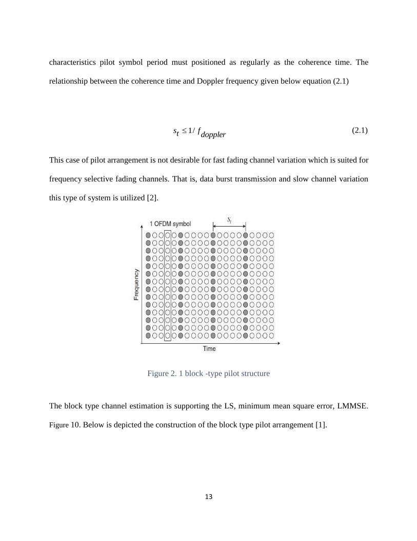
13
characteristics pilot symbol period must positioned as regularly as the coherence time. The
relationship between the coherence time and Doppler frequency given below equation (2.1)
dopplerfts /1 (2.1)
This case of pilot arrangement is not desirable for fast fading channel variation which is suited for
frequency selective fading channels. That is, data burst transmission and slow channel variation
this type of system is utilized [2].
Figure 2. 1 block -type pilot structure
The block type channel estimation is supporting the LS, minimum mean square error, LMMSE.
Figure 10. Below is depicted the construction of the block type pilot arrangement [1].

14
2.2.1 Least Square Estimator
The least square estimator is the basic technique for many channel estimation techniques
pilot data symbols are used for better performance, given N pilot subcarriers assume that's
orthogonal to each other. They are free of interference the pilot symbols for N subcarriers
represented by diagonal matrix [2].
X =
]1[00
0
0
0..0]0[
Nx
x
X (k) = pilot data at the Kth subcarrier where k = 0,1,2,……..N-1
Channel gain matrix H (k) at Kth subcarriers and the received pilot data at the receiver is given by
my (k) represented as
Y = XH+Z (2.2)
Channel vector H is given by H = [H (0), H (1), H (2),…… H [N-1]] T where Z is a noise vector
is given by Z = [Z (0), Z (0),…..Z (N-1)]. Let H is channel estimate of H
LS Estimation of Hlsp (K) at each subcarrier is given by
Hlsp (K) = Y (K) /X (K) (2.3)
To minimize the cost function H^ is given as J( H ) = ( HXY ˆ )2.
To determine the mean square error of the Hlsp is given by

15
MSElsp = E{(H- lspH )T (H- lspH )}. (2.4)
Simple least square estimation technique implemented in Simulink and Simulink BER curve by
using block type show in figure 2.2 below this are helpful with low complexity mean square error
is very high. This least square technique is implemented in DSP c6713DSK bit error rate is verified
[2].
Least square estimation BER cure in Simulink
Figure 2. 2 block LS estimation
2.2.2 Minimum Mean Square Estimation
In MMSE estimation here we are calculating the second order statistics of the channel to
minimize the MSE let g = [gn]T is sampled channel impulse response and n = [nn]
T
(0,………….N-1) is the AWGN channel noise matrix H = fftN( g ) = F g And N = F n and

16
corresponding auto covariance matrix are Rgg,,RHH and RYY and corresponding cross covariance
matrix is given by RgY, It is derived that.
RHH = E{ H HH } = F RggFH (2.5)
RgY = E{ g HY } = Rgg, FH XH (2.6)
RYY = E{ HYY } = XFRggFH XH + 2
N IN (2.7)
mmseg = RgY -1 YHH final MMSE estimation is given by Equation 8
mmseH = F mmseg (2.8)
Minimum mean square error greater performance, and so the least square estimation, but
it increases the complexity. Used in low SNR circumstances LMMSE are widely applied to cut
complexity [3].
2.3 Comb-Type
For this kind of arrangement, the pilot data symbol is regularly inserted for each block of
data symbols. During this phase of pilot arrangement pilot symbols are put in as frequently as
coherent bandwidth in frequency axis to follow the channel characteristics [2]. This coherence
bandwidth is reciprocally to maximum delay spread and the relationship between two are given
below equation (2.9)
max/1
fs (2.9)

17
Which are suitable for fast fading channels comb-type pilot structure is shown in figure 2.3. The
job here is to estimate the channel conditions at the data subcarriers. In comb type channel
estimation the solution includes the LS estimator with interpolation show in below sections
Figure 2. 3 comb-type pilot structure
2.3.1 LS Estimator with 1D interpolation
Pilot data symbols are inserted at a regularly Interval in actual block of data i. In specified
location here the channel estimation is done by using the interpolating the pilot data to the nearest
pilot data channel estimation is done by using the pilot interpolated data [1].
Linear interpolation (LI)
In this LI estimation first two nearest data points are interpolated this pilot interpolated data points
used estimate the channel this very simple method. This linear interpolation implemented in
Simulink

18
(2.10)
Here the comb-type channel estimation techniques in OFDM system using Simulink show in figure
2.4. Below SNR vs BER
Figure 2. 4 linear interpolation

19
2.3.2 Second Order Interpolation
Here we used three pilot carriers to estimate the second order Interpolation. This method
performs better than the least square Method Estimation based on a weighted linear combination
of the three adjacent pilot’s implementation second order interpolation show in below [4].
(2.11)
2.3.3 FIR Interpolation (LPI)
This method first it is inserting the zeros into the given interpolation location after that it
performs the interpolation mean square error is minimized with this method. Linear and FIR
interpolation using Simulink BER curve show in figure 2.5 below

20
Figure 2. 5 FIR Interpolation
2.3.4 Splice Cubic Interpolation (SCI)
The method produces a smooth and continuous polynomial fitted to given data points
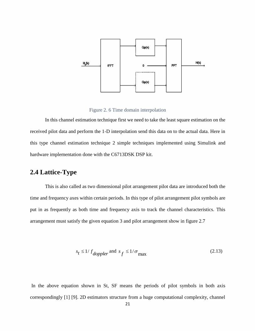
2.3.5 Time Domain Interpolation (TDI)
After finding the Hlsp first insert the zeros into original vector i.e. Zero padding and convert
into frequency domain into time domain and perform the piecewise linear interpolation and
converted back into frequency domain this is practiced in middle and low signal to noise ratio
environment[1].
21
Figure 2. 6 Time domain interpolation
In this channel estimation technique first we need to take the least square estimation on the
received pilot data and perform the 1-D interpolation send this data on to the actual data. Here in
this type channel estimation technique 2 simple techniques implemented using Simulink and
hardware implementation done with the C6713DSK DSP kit.
2.4 Lattice-Type
This is also called as two dimensional pilot arrangement pilot data are introduced both the
time and frequency axes within certain periods. In this type of pilot arrangement pilot symbols are
put in as frequently as both time and frequency axis to track the channel characteristics. This
arrangement must satisfy the given equation 3 and pilot arrangement show in figure 2.7
dopplerfts /1 and
max/1
fs (2.13)
In the above equation shown in St, SF means the periods of pilot symbols in both axis
correspondingly [1] [9]. 2D estimators structure from a huge computational complexity, channel

22
estimation based on the 2D least squares (LS) and 2D normalized least squares (NLS) are
suggested [1] [7].
Figure 2. 7 Lattice-type
23
CHAPTER 3
Adaptive Stochastic Gradient Algorithms
Implementation
3.1 Introduction
In previous chapter3 discussed about the mean square channel estimator’s one of the
greatest difficulties is that essential to estimate the covariance and cross covariance matrix of the
duct, which are not much available in nature, such a situation I need to cover the signal statistics
and need to calculate the signal statistics. Gradient algorithms abilities for learning and tracking
are the principal causes behind the broad role of this method in this chapter4, this learning
mechanism and tracking mechanism is possible to achieve by iterative schemes. One of the
methods is steepest-descent methods and fundamental of most adaptive filtering techniques. The
steepest - descent algorithm is given consider random vector u with Ru = Eu*u>0 and random
variable d with variance 2 and w0 is a weight vector [3].
W0 = this is the solution to the least square estimation problem
2min uwdE
w (3.1)
And recursively as follows begin with starting guess w-1 is generally 0 for our channel estimation
case and any positive step size is very small generally we considered and iterations i≥0.
iw = 1iw + µ[Rdu - Ru wi-1 ] (3.2)
wi → w0 and i → ∞

24
3.2 LMS Algorithm Implementation In Simulink
Consider a random variables d with realizations {d (0), d (1),……..}, And a random vector
u with realizations {u1, u2,………} the weight vector where u is a row vector wo is given by
2min uwdE
w
iw = 1iw +*
iu 1)( ii wuid , ,0i w-1 = initial guess
(3.4)
Generally, initial guess is zero and µ is very small which a positive value is
duu RRw10
(3.5)
The error is then used to regulate the filter coefficients form wi-1 to wi in keeping with. The error
signal can assume little values. The error signal is given as the difference between actual signal
and the desired signal [2].
M.m.s.e = 2 - duuud RRR1
(3.6)
The error is then used to adjust the filter coefficients from wi-1 to wi according to In steady-state,
the error signal will assume small values
LMS channel estimation in OFDM system using the Simulink show figure below. Received pilot
data are given to the LMS filter input and transmitter pilot data is given to LMS filter desired
signal. The step size is very small value selected. Let’s consider the },{ ii ud , are the input and
output of the OFDM system.

25
At every time instant I, the measured output of the channel, d (I), is compared with the yield of
the adaptive filter, =, and an error signal, we (I) = d (I) -, is generated.or signal, e(i) = d(i)- 1ii wu
, is generated. The error is then utilized to correct the filter coefficients.
In case of computational cost LMS need 2M real additions and 2M+1 real multiplications per
iteration is required for real valued data, for complex valued data 8M real addictions and 8M+2
real multiplication require . Weight adjustment is an important, weight adjustment is as minimum
as possible get the desire signal output of adaptive filters. Adaptive filter efficiency depends on
the several iteration this iteration as many as possible generally considered. LMS algorithm can
work stationary or non-stationary. In Simulink, it is very simple to make an LMS channel
estimation model using Simulink show in figure 3.1 below. Here step size is taken as 0.1.figure
3.2 shows the BER curve.
Figure 3. 1Simulink LMS algorithm model

26
Figure 3. 2 Simulink LMS channel estimation BER curve
3.2.1 Advantages
1. Simplicity
2. Robustness
3. Low computational complexity
3.2.2 Applications
Adaptive channel estimation
Adaptive channel equalization
Decision feedback equalization

27
3.3 NLMS Algorithm In Simulink
Consider a random variables d with realizations {d(0),d(1),,……..}, And a random vector
u with realizations {u1, u2,………} the weight vector where u is a row vector wo is given by
2min uwdE
w (3.7)
Approximated NLSM is given by
)0(,,0],)([/ 11
*2
1 guessinitialwiwuiduuuww iiiiii (3.8)
ε is a small parameter (positive)
the newton’s regularization ε(i) an µ(i) are constant
][][ 1
1
1
iuduuii wRRRIww (3.9)
NLMS recursion
,0],)([/ 1
*2
1 iwuiduuwwi iiiii (3.10)
In case of the NLMS computational cost it requires the 3M real additions, 3M+1 real
multiplications and one real division require in our algorithm case complex valued case for this
10M real addition, 10M+2 real multiplications and one real division [3].
NLMS has a computational complexity, higher than the LMS, but the advantage is that
converges faster than LMS. In normal case LMS creates a problem LMS require the large

28
information (pilot) to estimate the channel. µ is normalized in such a way that energy of data
vector.
3.4.1 Application
1. Echo cancellation and noise reduction
NLMS OFDM channel estimation using Simulink and it’s SNR vs BER curve show in the figure
3.2 same as the LMS algorithm with the varying step-size.
3.3 RLS Algorithm Using Simulink
RLS adaptive filter is an algorithm which recursively finds the filter coefficients that
minimize least squares cost function RLS has extremely fast convergence but computational
complexity increases and good tracking performance [3].
Consider a random variables d with realizations {d(0),d(1),,……..}, And a random vector u with
realizations {u1, u2,………} the weight vector where u is a row vector wo is given by
2min uwdE
w
Regularization newton’s method
][])()[( 1
1
1
iuii wRRduRuIiiww (3.11)
Replace 1 iudu wRR (3.12)
Approximation
][* 1 iii wudui (3.13)

29
For better estimation Ru
i
j
jj
ji
u uuiR0
*1/1ˆ (3.14)
λ= 1
And so the above equation becomes
i
j
jju uuiR0
*1/1ˆ (3.15)
ui most recent regression is require to update the p i-1 to pi
Iteratively through recursion
(3.16)
The RLS algorithm is associate order of magnitude costlier than LMS-type algorithms,
requiring O(M2) vs.O(M) operations per iteration. However, RLS
converges considerably quicker than LMS t's familiar that the RLS filter converges quicker than
the LMS filter generally, however, that if you are following time varied parameters the LMS
algorithm perform higher. LMS filter is sort of a purpose estimate, however the RLS
uses additional data. RLS has fast convergence compare to other algorithms and full tracking
capability. When it comes to RLS channel with ε = 0.995 and variance = 1 the algorithm

30
producing high computational complexity and corresponding response curve is drawn between
BER and SNR is as shown in the figure [3.3].
The performance of the RLS algorithm depending on the parameter ε for number of
observations and number of iterations in RLS the mean value keep on decreasing and become the
constant theoretically [3].
Figure 3. 3 RLS performance curve

31
Chapter 4
Hardware Implementation of OFDM
Channel Estimation Techniques Using
C6713DSK
4.1 Introduction
Real time digital signal processing give a guaranteed of delivery of data in certain time
keep pace with some external events in non-real time case does not have the such time
constraints.DSP have cost effective compare to the compare to the other processor depending on
the application.DSP are less effected by the environmental changes this are easy to use and flexible
general DSP’s are more useful for audio signals which is 0 to 90khz general DSP consist of ADC
which is used to capture the input signal this signal processed and converted to DAC converter
Processing of analog signals can be done in either in analog or digital domain. In analog
communication response to various physical phenomena in analog manner i.e. in continuous time
and amplitude.in order to convert the analog signal to digital signal digitizing is used perform via
an analog to digital converter. The reason behind the using of DSP’S are those are used to allow
the programmability DSP C6713DSK used many application by changing the simple code.DSP’S
are more stable and tolerant output then the analog communication system. Present world DSP’s
play major role in the 3G wireless, cable modems, and DSL modems. The processing digital
signals can be implemented in different domains like DSP’s and VLSI circuit, microprocessor
[13].

32
4.2 DSK Support Tools
4.2.1 Required Software and Hardware
DSK6713 starter kit is need for code generation and to test the data at input and output are
function generator, microphone, cables with audio jacks and oscilloscope USB cable to connect
the DSP to PC’s. Software is needed to execute the generated code called code composer studio
(CCS). In this CCS application consist of compiler, assembler, linker simulator, and debugger
utilities [13].
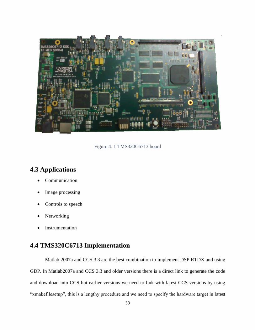
4.2.2 DSK Board
16MB-SDRM and 256KB flash memory Input and output MIC IN, LINE IN are input ports
MICOUT, LINEOUT output ports The DSK features the TMS320C6713 DSP, a 225 MHz device
delivering up to 1800 million instructions per second c6713 internal memory of 256KB c6713
perform the both floating point and fixed point operations, JTAG interface through USB figure 4.1
below shows the TMS320C6713 starter kit and it’s applications [13].
33
Figure 4. 1 TMS320C6713 board
4.3 Applications
Communication
Image processing
Controls to speech
Networking
Instrumentation
4.4 TMS320C6713 Implementation
Matlab 2007a and CCS 3.3 are the best combination to implement DSP RTDX and using
GDP. In Matlab2007a and CCS 3.3 and older versions there is a direct link to generate the code
and download into CCS but earlier versions we need to link with latest CCS versions by using
“xmakefilesetup”, this is a lengthy procedure and we need to specify the hardware target in latest

34
CCS versions. CCS3 and below versions do not support for windows7 users better to exit switch
to CCS4/CCS5 with MATLAB 2011a are the best shapes [13].
DSP’s are super-efficient compared to the PC’S executing the signal processing
algorithms, hence they are of great use in the industry when it adds up to the simple display PC’S
much better than DSP’S For example, you want to do any complex model it will execute 10 times
quicker than the PC’S but doesn’t supply us any form of visual display unit but there is even a
chance of making the output using RTDX and GDP. Information exchange between the DSP and
computer two way communication channel is methodology this setup is implemented in this thesis
[13].
4.5 OFDM Hardware Implementation Using c6713DSK
As shown in the figure 1.2 chapter1 OFDM implementation using Simulink models with
hardware implementation setting and running model show. This OFDM transceiver model with
16-QAM rectangular modulation, 56 symbols and 8 pilot carriers are in frequency domain. 64 –
point IFFT convert the frequency domain to time domain last 16 bits of data is added to the
beginning of the data to make the cyclic prefix and serial to parallel conversion is done. At the
receiver remove the cyclic prefix and perform the FFT with same 64-point and pilot data is
separated here to estimate the channel, data symbols are sent to the error rate calculatorfigure1. 2
chapter 1. Select the target preference and select the settings accordingly. Select the “to RTDX “
to produce the desired response connects this block to get DSP output RTDX is generally applied
to transpose the data between the aim to the Matlab by using JTAG emulator, my job is to count
on the BER. RTDX is connect to error rate calculator and build the model by changing the solver
settings accordingly. Plug in the PC to the c6713DSK using USB cable, open the Matlab and to

35
determine the CCS is installed properly or not for this in Matlab command window type
“ccsboardinfo” it returns information “board type “ and “processor name”. To follow out any
model proper hardware configuration selection is very important, This model implemented with
windows Xp Matlab7 and CCS3.3 this is the best combination another one combination is
windows 7, Matlab2011a with CCS4/CCS5.Ones done all these settings you real-time workshop
converts Simulink models into ASIC C/C++ code that can compile using CCS. Link for CCS is
used to invoke the code building process from within CCS to build an executable. This code can
then be downloaded to the target DSP from where it flows. The data on the target is accessible in
CCS or in Matlab via Link for CCS or via Real-Time Data Transfer (RTDX). This thesis primarily
uses RTDX for accessing information on the target DSP. Two ways to control the DSP output
discussed in below section with OFDM implementation [13].
4.6 Experimental setup and Simulink model
The below figure 4.2 indicate that the experimental setup and Simulink model of OFDM system
with channel estimation techniques. The hardware setup required the PC’s and c6713DSK KIT and
connecting wires. Power on the DSP kit with the adapter cable, connect the PC’s to the TMS320C6713
hardware kit with the USB cable. Go over the connector on the PC. And check also in MATLAB by using
the function “ccboardinfo” once you connect the hardware go to Simulink and run the model select the
configurations according to the application and build the model and generate the code to target hardware it
will automatically generate the code and automatically. You can free to see the code in CCS and see the
output by using RTDX [12].

36
Figure 4. 2 hardware setup
4.7 c6713DSK – Matlab Link Using the RTDX
Two ways to exhibit the output one way is by utilizing the DSP MATLAB code and another
one is using GDP here the simple program for open the RTDX given below. Two types RTDX
channel is available in Simulink one is ‘to RTDX’ and ‘from RTDX’ one is used for sending/write
from PC’s to DSP’S and another channel is used receive/read the data from the DSP. Here I used
‘to RTDX’ to get the DSP output.
4.7.1 Link uses RTDX cc = ccsdsp;
open(cc.rtdx,'ochan2','r')
%od = zeros(1.1000);
for k = 1:10000

37
%od(1:end-1) = od(2:end);
%od(end) = readmsg(cc.rtdx,'ochn1','double',1)
od = readmsg(cc.rtdx,'ochan2','double',1);
plot(od);
drawnow;
end
4.7.2 Using External Application
This application is used to get the numerical results using little window show in figure 4.4
below with DSP output. GPD used to add the channel to provide interface this application available
in the CCS Folder itself here tested results show in figure 4.3. Below with OFDM resultant
received data bits and errors in DSP6713. And also code generation part is also shown in figure 4.
3 Below.

38
Figure 4. 3 code generation part
Figure 4. 4 GPD output

39
4.8 Channel Estimation Techniques, Implementation in C6713dsk
In this thesis block-type and come-type channel estimation techniques are discussed. Basic
and fundamental channel estimation technique least square estimation using block-type and comb-
type are discussed and implemented in c6713DSK with the help of RTDX and GDP bit error rate
is computed. Implemented and efficiency of the system estimated. Block type channel estimation
techniques are complexity increases and these are suitable for slow type channel variations. Below
figure 4.5. DSP hardware implementation and it’ bit error rate curve [13].
Figure 4. 5 setup diagram of interpolation channel estimation
Hardware implementation is done using c6713DSk kit with the help of external application like i
mentioned in this chapter and below figure 4.6 shown below

40
Figure 4. 6 DSP bit error rate
Presents the results for SNR=20dB and for SNR=10 dB. In both cases LMS, NLMS and
RMS has performance that compares very favorably with the other two algorithms but with a very
appealing computational complexity. In Fig. 4.7 we also plot the performance of the adaptive
algorithms using less step size. We present the bit error rate (BER) of the RLS, LMS NLMS
scheme with perfect channel knowledge, for different values of the SNR. We observe an
indistinguishable performance of the adaptive schemes as compared to the one with perfect
channel knowledge.

41
Figure 4. 7 LMS, NLMS, RLS, setup diagram

42
Chapter 5
Conclusion
5.1 Conclusions
In this thesis, a performance comparison between the different channel techniques based on
the pilot arrangement is investigated. Comb-type channel estimation techniques are implemented
in Simulink and compared with different interpolation techniques. Complexity increases in comb-
type and block-type algorithms for that we estimated the other channel estimation techniques in a
simple way to reduce the complexity. LMS, NLMS, and RLS are the Compared with the other
channel estimation techniques and also compared LMS, NLMS, and RLS algorithms with different
step-sizes using the SIMULINK models. Compared with the three algorithms RLS has high
performance RLS algorithms has a high perform. And also implemented this algorithms in the real
time implementation using the TMS320C6713 DSP by transferring Simulink model to the DSP
c6713DSK kit with the help of CCS and verified the output with the help of the RTDX. This thesis
focuses on channel estimation with different interpolation approaches and adaptive algorithms
OFDM system.
5.2 Future work
The future works that can be conducted on the technique are deduced from the drawbacks of
the techniques. Two dimensional estimations techniques more efficient then the above techniques
but complexity increase.

43
References
[1] M. K. Ozdemir and H. Arslan, “Channel Estimation for Wireless OFDM Systems,” IEEE
Communications Surveys & Tutorials, vol. 9, no. 2, pp. 18-48, 2nd Quarter 2007.
[2] Henrik Schulze, Christian Luders, “Theory and Applications of OFDM and CDMA
Wideband Wireless Communications”, John Wiley & Sons Ltd., chap 4, pp 145-160, 2005
[3] Ali H. Sayed, Adaptive Filters, Wiley, NJ, 2008[13] (ISBN 978-0-470-25388-5).
[4] Van de Beek, J.J., Edfors, O., Sandell, M. et al. (July 1995) On channel estimation in OFDM
systems. IEEE VTC’95, vol. 2, pp. 815–819.
[5] Hsieh, M. and Wei, C. (1998) Channel estimation for OFDM systems based on comb-type
pilot arrangement in frequency selective fading channels. IEEE Trans. Consumer Electron.,
44(1), 217–228.
[6] Tufvesson, F. and Maseng, T. (May 1997) Pilot assisted channel estimation forOFDMin
mobile cellular systems. IEEE VTC’97, vol. 3, pp. 1639–1643.
[7] Fernandez-Getino Garcia, M.J., Paez-Borrallo, J.M., and Zazo, S. (May 2001) DFT-based
channel estimation in 2D-pilot-symbol-aided OFDM wireless systems. IEEE VTC’01, vol. 2, pp.
810–814.
[8] Hu, D. and Yang, L. (Dec. 2003) Time-varying channel estimation based on pilot tones in
OFDM systems. IEEE Int. Conf. Neural Networks & Signal Processing, vol. 1, pp. 700–703.
[9] Li, Y., Cimini, L. Jr, and Sollenberger, N.R. (1998) Robust channel estimation for OFDM
systems with rapid dispersive fading channels. IEEE Trans. on Commun., 46(7), 902–915.
[10] Tang, Z., Cannizzaro, R.C., Leus, G., and Banelli, P. (2007) Pilot-assisted time-varying
channel estimation for OFDM systems. IEEE Tran. Signal Processing, 55(5), 2226–2238.
[11] Rohling, H. and Grunheid, R. (May 1997) Performance comparison of different multiple
access scheme for the downlink of an OFDM communication system. IEEE VTC’97, vol. 3, pp.
1365–1369.
[12] Bertrand Muquet, Member, Cyclic Prefixing or Zero Padding for Wireless Multicarrier
Transmissions? IEEE, Zhengdao Wang, Student Member, IEEE, Georgios B. Giannakis,Fellow, IEEE,
Marc de Courville, Member, IEEE, and Pierre Duhamel, Fellow, IEEE.
[13] Chassaing, Rulph. Digital Signal Processing and Applications with the C6713 and C6416
DSK. Vol. 16. John Wiley & Sons, 2004.
44
[14] Yuping Zhao, Aiping Huang, “A novel channel estimation method for OFDM mobile
communication systems based on pilot signals and transform-domain processing ,” IEEE VTC ,
Vol. 3, May 1997.
[15] Simeone, Osvaldo, Yeheskel Bar-Ness, and Umberto Spagnolini. "Pilot-based channel
estimation for OFDM systems by tracking the delay-subspace."Wireless Communications, IEEE
Transactions on 3.1 (2004): 315-325.
[16] Colieri, Sinem, et al. "A study of channel estimation in OFDM systems."Vehicular
Technology Conference, 2002. Proceedings. VTC 2002-Fall. 2002 IEEE 56th. Vol. 2. IEEE,
2002.
[17] Yang, Baoguo, et al. "Channel estimation for OFDM transmission in multipath fading
channels based on parametric channel modeling." Communications, IEEE Transactions on 49.3
(2001): 467-479.
[18] M. Morelli and U. Mengali, “A comparison of pilot-aided channel estimation methods for
OFDM systems,” IEEE Transactions on Signal Processing, vol. 49, no. 12, pp. 3065-3073, Dec.
2001.
Online Resources:
1. www.ti.com – Official Website of Texas Instruments
2. www.wikipedia.org
3. http://www.mathworks.in/products/simulink/
4. www.google.com – Search Engine for data and images