CALCULATION OF DIFFRACTION EFFECTS ON THE AVERAGE PHASE OF AN OPTICAL FIELD

Miltiadis V. Papalexandris, David C. Redding

Jet Propulsion Laboratory California Institute of Technology

Pasadena, CA 911 09

1

Keywords

Diffraction Modeling, Fresnel Diffraction, Paraxial Equation, Discrete Fourier Transform

Person to whom proofs are to be sent

Miltiadis V. Papalexandris Jet Propulsion Laboratory

California Institute of Technology Mail Code: 306-336 Pasadena, CA 91109 Tel: (818) 354-1292 Fax: (818) 393-4773

milto@hive.jpl.nasa.gov

2

Abstract

The present paper reports on algorithms for the computation of the av- erage phase of a beam over a detector in the near field. This work is part of the diffraction modeling efforts for the Space Interferometry Mission (SIM). The basic idea is to reconstruct the optical field numerically and then use a quadrature algorithm to evaluate the quantity of interest. The various algorithms that employ discrete Fourier transform techniques for the compu- tation of the field are described and numerical tests that assess the accuracy of these algorithms are presented. There is not one particular algorithm that delivers the desired accuracy over the entire range of Fresnel numbers of interest, but each one can produce satisfactory results within a particular range. Finally, new methods to evaluate the average phase are introduced and their efficiency is assessed.

Introduction

Diffraction is one of the fundamental subjects in optics because of its theoretical interest and its practical applications. For most cases the far- field approximation, Fraunhoffer diffraction, provides a sufficient framework of analysis. There are cases, however, where near-field diffraction effects are important.

Such cases abound in the Space Interferometry Mission (SIM), a part of NASA’s Origins program. Applications that require near-field diffraction calculations include the calibration of measurements of the internal metrol- ogy system, modeling of corner cube effects, starlight-system modeling etc. Highly accurate diffraction calculations, down to the picometer level, are necessary in all these applications.

The quantity of interest is the average phase of the field over an optical element, usually a detector. Typically, its computation consists of two steps. The first one is the reconstruction of the optical field and the second one is the numerical integration of the field over the element. The present study is concerned with the available algorithms for both steps.

The boundary value problem that governs free-space beam propagation in the near field has been studied extensively and results can be found in standard textbooks, e.g., Goodman [l]. In the past, many different methods have been proposed for evaluation of near-field diffraction integrals. One such method is based on local approximation techniques of the integrand;

3

see, e.g., Stamnes et al., [ a ] , D’Arcio et al., [3], and others. Other methods rely on numerical integration. Examples of this approach are the algorithm of Southwell, [4], which employs Gaussian quadrature, and the algorithm of Kraus, [ 5 ] , which is based upon a finite-element formulation of the diffraction integral. Approximate procedures that require less computing time have also been presented. Such procedures have been employed in the asymptotics- based scheme of Horwitz, [6], and the scheme of Carcole e t al., [7], which is based on approximations of the diffraction integral with simpler ones that admit a closed-form representation.

Over the years, dicrete Fourier transform methods have become a pop- ular choice for near-field diffraction calculations. Such methods have been developed by Sziclas & Siegman, [8], Mansuripur, [9], Mendlovic et al., [lo], and others. More recently, Mas et al., [ll], proposed an algorithm based on the fractional Fourier transform. The main advantages of Fourier-based methods are easy implementation, robustness, and speed.

As mentioned above, the second step for the computation of the average phase is the numerical integration of the field. The errors that are introduced during this step might be substantial. In principle, the integration can be performed via the multi-dimensional extension of quadrature rules such as Simpson’s rule, Gaussian integration, and others.

The first objective of this work is to compare the performance of exist- ing Fourier-based algorithms under very high accuracy requirements. These algorithms are described below in some detail for completion purposes. The regimes of their effectiveness are explored through a series of tests. Studies of the performance of these algorithms with such high accuracy requirements have not been previously reported in the literature. The effectiveness of various techniques for numerical integration of the field is also discussed.

The second objective is to propose new methods for the evaluation of the average phase. More specifically, for oversized elements an exact closed-form solution is derived. Finally, a new, hybrid algorithm for the average phase is introduced. It is based on an inherent reciprocity property of the quantity of interest and the partitioning of the optical element to rectangular elements.

Formulation and Solution of the Boundary Value Problem

The free-space beam propagation problem is formulated as follows. Con- sider an isotropic, homogeneous, nondispersive and non-magnetic medium covering the half space SI ( x , y, z 2 0). Further, consider an aperture,

4

denoted by r, at the plane x = 0, emitting plane waves of wavelength X. The generated optical field can be fully described by a scalar complex function, U , satisfying the scalar Helmholtz equation,

( ax2 ay2 az2 ) a2 a 2 a 2 -+-+-+IC2 U ( x , y , z ) = 0 , ( x , y , x ) E . Q , (1)

a Dirichlet condition at the boundary z = 0,

and the Sommerfeld radiation condition at infinity,

In the above system, k is the wave-number, defined as k = 27r/X. R is the distance of the point of observation ( x , y, z ) from the origin, and j is the imaginary unit. The Sommerfeld radiation condition sets the boundedness requirement for the solution and determines the direction of propagation of the waves. At infinity they should be travelling away from the aperture, Goodman [ 11.

The problem can be solved by applying the Fourier transform in the x and y directions, then solving the resulting Ordinary Differential Equation (ODE), and finally applying the inverse Fourier transform. The result is given by

+cm

"00

where

is the Fourier transform of the field at the boundary z = 0. It is usually called "the angular spectrum" of the field. In the sequel, the above expression is referred to as the first integral representation of the optical field.

5

An alternative way to obtain the solution is to make use of Green’s the- orem. This approach is often called the “point source” method. The result is the well-known Rayleigh-Sommerfeld diffraction formula,

where 7-01 is the distance of the point of observation ( x , y, z ) from a point ([, 7) inside r,

7-01 E 4 2 2 + (a: - + (y - q)2

This is the second integral representation of the optical field. One can take advantage of the fact that the boundary data are identically zero outside the aperture I? and extend the limits of integration to infinity. The two representations, (4) and (6), are completely equivalent, Le., they result in identical fields. Further, the first representation can be deduced from the second one by direct application of the convolution theorem.

The well-known Fresnel approximation arises when the square roots in the arguments of the complex expenentials of the above expressions are replaced by the first two terms of their binomial expansions. In other words,

and

Relation (8) can be substituted into (4). Relation (9) can be substituted into the complex exponential in (6). For equation (6) and for propagation dis- tances much larger than the aperture dimensions, it can further be assumed that z/r& = 1/z and ( j k - l/rol) N jlc. The result is

u (x ,y , x ) = ejkz j- F(f X ? f y , 0) e - j X x z ( f z + f $ ) ejas(fxX+fgY) d f x d f y , (10)

“00

and

“00

6

respectively. It can be readily verified that the above expressions, without the geometrical phase term, are the solution of the paraxial equation, i e . ,

( ax2 dy2 d x ” ) d2 a 2 - + - + j 2 k - q x , y, x ) = 0 , ( x , y, x ) E s2 , (12)

with

U ( X , y, x ) = ejkz ~ ( x , y, x ) ,

and boundary condition for U given by (2). The Fresnel approximation is often called the paraxial approximation. Its validity for modeling diffraction effects at the required accuracy level is discussed below.

Near-field diffraction algorithms are based on numerical integration or approximation of either (10) or (11). Methods that solve equation (10) nu- merically are usually referred to as angular spectrum methods. The use of Fast Fourier Transform (FFT) for the calculation of the Fourier integrals ap- pearing in (10) results in a powerful and robust solver. Its computational cost is proportional to that of two 2-D FFT’s. Guard-band ratio requirements, based on approximations of the integrals involved, have been introduced in [8] and [9], to avoid aliasing and energy spill-over to the computational domain.

Equation (11) is also a Fourier-type integral, therefore FFT may be em- ployed for its computation. This method requires only one 2-D Fourier trans- form. However, the scaling factor 1/Xx that appears in the Fourier kernel introduces certain computational problems that are described later in the paper. The accuracy of the method was examined in [lo], and it was found to be satisfactory for sufficiently large propagation distances. Additional nu- merical tests performed in the context of the present study, also indicate that this method produces reasonable results. However, if the error tolerance is very small, this method is not recommended, even for large distances.

A robust method to solve equation (11) numerically is to approximate the integral by a Fourier series whose sum can be computed with the Goertzel- Reinsch algorithm, Stoer & Bulirsch [12]. This algorithm performs simul- taneous summation of sine and cosine series by employing the Clenshaw’s recurrence formulae that hold for trigonometric functions. One of the advan- tages of this method is that there is freedom in the choice of the sampling intervals at the ( x , y) plane where the field is computed. In contrast, there is no such freedom if FFT is employed. In the sequel, this method will be referred to as the direct method.

7

The critical parameter for the problem under consideration is the Fresnel number, defined as

W2

Ax Fr = -,

where w is the characteristic semi-length of the aperture. Simple examination of equations (10) and (11) reveals that the integrand in (10) becomes more oscillatory as the Fresnel number decreases, while the opposite holds for the integrand in (11). Therefore, with fixed grid sixes, the accuracy of the angular spectrum approach is improving as the Fresnel number increases, while the opposite is true for the direct method.

It should be mentioned that, in principle, other methods can be employed for the numerical integration of equation (11). Such methods are gaussian and Clenshaw-Curtis type quadratures. The later method is based on Cheby- chev polynomial approximation of the integrand, Clenshaw & Curtis, [13], and Littlewood & Zakian, [14]. The main disadvantage of these algorithms is that they can not be employed in equispaced grids, see also the discussion below. Equispaced grids are very convinient in diffraction modeling because beams can be propagated from element to element in a straightforward man- ner.

A method that works with uniform sampling is Filon-type quadrature, Levin [15]. This method transforms the integration problem to an O.D.E. problem that is solved by a collocation technique. Its main disadvantage is that it requires the solution of a linear system of equations (the colloca- tion conditions), which makes it slow. On the other hand, discrete Fourier transforms combine robustness, speed, and straightforward implementation. Therefore, they are very effective for the calculation of diffraction integrals.

Calculation of the Average Phase of the Field

The quantity that has to be evaluated with high accuracy is the average phase of a beam over an optical element, A. This element is usually a detec- tor. The average phase is defined in a way that is compatible to the process of interferometric measurements. Consider a beam of unknown amplitude and phase distributions, combined with a reference signal of constant amplitude and phase. The average phase is evaluated via intensity measurements of the combined beam at the detector. If the properties of the reference signal are

8

known, the measured intensity depends only on the real and imaginary part of the integral of the unknown beam over the detector.

Therefore, the average phase is defined as the phase of the integral of the field over A,

I = /U(x, y,z) dxdy. A

In computer modeling cp can be evaluated directly from the above relation via numerical quadrature, provided the field U(x, y) is known. Algorithms such as the two-dimensional extension of Simpson’s rule or Romberg integration are quite often sufficient for such task.

A very effective way to compute I is Gaussian quadrature. Gauss-Legendre integration, for example, is superior to any elementary algorithm such as Simpson’s rule. It is also very simple and easy to program. Its main dis- advantage is that the abscissas are not equispaced. Therefore, it can not be employed to fields evaluated from FFT-based algorithms. For this rea- son, the numerical integration of the field was not performed with gaussian qudrature.

Application of the convolution theorem provides another way to compute I on an orthogonal grid. The procedure is the following. Denote by A(x - [, y-q) the optical-element function of A with origin at (e, q ) , not necessarily its geometric center. Consider the cross-corellation integral

which, in view of the convolution theorem, becomes

The quantity of interest, I , is equal to the zero-frequency component of G. It can be computed by numerical integration, say via Simpson’s rule of the product of the Fourier transforms of U and A. In other words, computation of the full inverse transform G is not necessary. Numerical tests showed that

9

for large Fresnel numbers this is the most accurate quadrature method on equispaced grids. At low Fresnel numbers its accuracy is similar to that of Simpson's rule.

Numerical Tests

The performances of the angular spectrum method and the direct method have been examined through a series of numerical tests. The tests consisted of beam propagation from a square aperture to a square detector; see figure 1. The beam at the aperture had uniform phase and intensity, equal to one. The geometry was kept as simple as possible so that closed-form solutions for the optical field can be used for comparisons.

It is well known, [l], that in the context of Fresnel diffraction the field generated by a square aperture of width 2w is given by

ejkz W J - 7 Y, 4 = - [C(a2) - C(W> + j(S(Q2) - S(Ql>>] x

2 j W 2 ) - W 1 ) + M P 2 ) - S(P1))I 7 (19)

where the functions C and S are the Fresnel integrals, Gradshteyn & Ryzhik [16], and

Q1 = -(w + X ) r n , Q2 = ( w -X)dqTz,

This equation is the exact solution for the paraxial equation with square aperture. The Fresnel integrals appearing above can be computed with dou- ble precision accuracy via standard algorithms; see, for example, the JPL library math. j p l . nasa. gov.

First, the field was computed with the above closed-form solution. Then, the integral of the field over the detector was evaluated with Gauss-Legendre quadrature. The number of points used in the quadrature was successively multiplied by a factor of 2 until a convergence of rads or better has been observed. Typically, 512 points on each grid direction were sufficient to provide the required accuracy. Henceforth, this result will be referred to as the closed-form result of the average phase. It is the reference result which numerical integration algorithms was compared with.

10

Next, the field was computed with the algorithms described above. It was assumed that the Fresnel approximation is valid. Hence, the field is governed by the paraxial equation and its integral representations are given by equations (10) and (11). The average phase over the detector was evalu- ated by applying the two-dimensional Simpson’s rule on the computed field. Henceforth, these results will be referred to as the numerical results. The error on the calculation of the average phase as a fraction of a wavelength was measured in picometers. For example, a 27r error in the average phase is said to be an error of one wavelength. Similarly, a convergence of rads in the computation of the closed-form result corresponds to accuracy at the level of 2% of a picometer, for the wavelengths of interest. Any error in the computation of the average phase larger than 20 picometers is considered unacceptable for the SIM modeling efforts.

Three different sets of parameters were considered. Double precision arithmetic has been used throughout. The computations were performed on a SUN ULTRA-10 workstation, at the finest grid that the machine could provide. The grid size for the angular spectrum method was set at 2048 X 2048 points. Different guard-band ratios had been examined in all test cases con- sidered. The results that are included in the present work have been obtained with the guard-band ratio that delivered the highest accuracy for each case. The grid for the direct method had been set at 512 X 512 points.

Case A corresponds to the starlight system of SIM. The parameters for this case are

X = 0.7pm, 2w = 3.0cm, 2W = 6.0cm, x = 7.0,. . . ,9 .0m,

where w is the half-width of the aperture and W is the half-width of the detector. The Fresnel number of this problem is F r N 46.0 at z = 7m. Figure 2 shows intensity and phase plots at (y = 0, z = 7m), as computed from the closed-form solution (19).

The angular spectrum algorithm proved quite effective, yielding maxi- mum error of 13.7 picometers, or 0.002 % of the wavelength, at z = 8.7 m. This error is, therefore, acceptable for the SIM modeling requirements. The guard-band ratio at the aperture was set to 4. Numerical jitter was minimal with such zero-padding. Different guard-band ratios were also tested. Lower ratios gave less accurate results due to energy spill-over in the computational domain. For example, a ratio value of 2 yielded maximum error of 27.5, at z = 8.8m. On the other hand, higher ratios dictated fewer points inside the

11

detector, which implies lower resolution for the numerical integration of the field. Consequently, the accuracy of the results dropped when higher ratios were used. With a guard-band ratio equal to 8, the maximum error was 27 picometers at z = 9 rn.

The direct method produced results that were considerably less accurate, see figure 4. The maximum error was encountered at z = 7.85 m and it was equal to 149.5 picometers. Such error is too high for the modeling require- ments of SIM. Therefore, the use of this method is not recommended for such high Fresnel numbers.

Case B is representative of the internal metrology system of SIM. The parametrs for this case are

X = 1.3prn, 2w = 5.0.rnrn, 2W = lO.Ornrn, z = 10.0,. . . ,12.0m.

Intensity and phase plots of the optical field at (9 = 0, z = 10 r n ) are shown in figure 5 . The Fresnel number for this case is Fr N 0.48 at z = 10m, considerably smaller than the first case. Nonetheless, this is not a far-field diffraction case; computation of the Fraunhoffer diffraction integral, [l], pro- duced results that were innacurate.

The function inside the first integral representation of the field has become more oscillatory because the Fresnel number has been lowered. As a result, the angular spectrum method becomes less accurate. The maximum error was 714 picometers, at z = 11.95rn, well beyond the error tolerance level. The guard-band ratio for this case was set to 8. Even with such high zero padding, the wavefront profiles suffered from some jitter due to energy spill- over in the computational domain.

Different guard-band ratios yielded even less accurate results. For exam- ple, when the ratio was lowered to 4, the error peak was 2164 picometers at z = 10.95 rn. The increase in the error is due to numerical jitter on the numerically evaluated field. On the other hand, larger guard-band ratios resulted to insufficient resolution for the numerical integration of the field. When the ratio was set at 16, the error peak was 895 picometers at z = 12 rn.

In contrast, the direct method gave results that were extremely accurate. The integrand in equation (11) is well-resolved with the sampling at the avail- able grid size, 512 points at each grid direction. This was expected because this function becomes less oscillatory as the Fresnel number decreases. The error peak was 0.48 picometers at z = 11.35 rn.

12

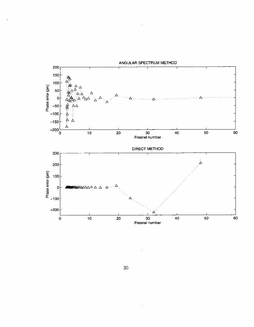
On a different test, the propagation distance varied from 0.05 m, to 2.2 m (on increments of 0.05 m), corresponding to a Fresnel number variation be- tween 0.96 to 2.18, approximately. The phase errors of the two algorithms as a function of the Fresnel number are shown in figure 8. For Fresnel numbers larger than 20, the angular spectrum method is very accurate and superior to the direct method. At lower Fresnel numbers the accuracy drops at the order of 200 picometers. The guard band ratio was set at 4.

On the other hand, the direct method is extremely accurate for Fresnel numbers smaller than 20. At larger Fresnel numbers, its accuracy deterio- rates rapidly. When the Fresnel numbers becomes higher than 50, the errors of the direct method are at the order of nanometers. This is due larger er- rors in the computation of the field, created by insufficient resolution at the aperture. Over all, the required accuracy can always be achieved if the an- gular spectrum method is employed at high Fresnel numbers and the direct method at lower ones. The cross-over point is around F r = 20.

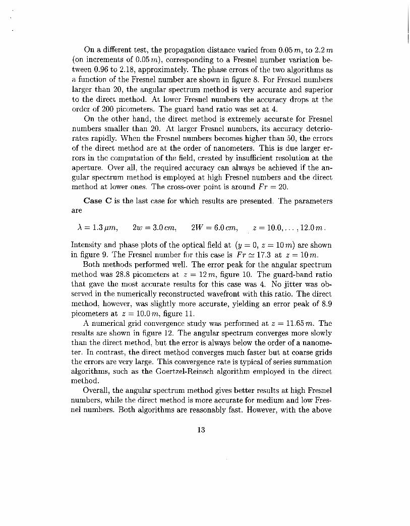
Case C is the last case for which results are presented. The parameters are

X = 1.3,um, 2w = 3.0cm, 2W = 6.0cm, z = 10.0,. . . ,12.0m.

Intensity and phase plots of the optical field at (y = 0, x = 10m) are shown in figure 9. The Fresnel number for this case is Fr N 17.3 at z = 10m.

Both methods performed well. The error peak for the angular spectrum method was 28.8 picometers at z = 12 m, figure 10. The guard-band ratio that gave the most accurate results for this case was 4. No jitter was ob- served in the numerically reconstructed wavefront with this ratio. The direct method, however, was slightly more accurate, yielding an error peak of 8.9 picometers at x = 10.0m, figure 11.

A numerical grid convergence study was performed at x = 11.65 m. The results are shown in figure 12. The angular spectrum converges more slowly than the direct method, but the error is always below the order of a nanome- ter. In contrast, the direct method converges much faster but at coarse grids the errors are very large. This convergence rate is typical of series summation algorithms, such as the Goertzel-Reinsch algorithm employed in the direct method.

Overall, the angular spectrum method gives better results at high Fresnel numbers, while the direct method is more accurate for medium and low Fres- nel numbers. Both algorithms are reasonably fast. However, with the above

13

grid sizes the angular spectrum method is still faster. In modern worksta- tions, one calculation of the average phase takes a fraction of a minute. In conclusion, the desired level of accuracy can be achieved for a wide range of Fresnel numbers, with appropriate choice of algorithm.

It should be mentioned that the use of FFT for calculating equation (11) was also tested. This is the fastest possible algorithm because it requires only one FFT. The computations were performed on a 2048 x 2048 grid at the aperture. The results, however, were not satisfactory. In all the test cases considered, the error peaks were at the order of a nanometer. The reason for such high errors is the following.

Suppose that the grid size at the aperture is N x N and that the Sam- pling interval is A t . Then, the sampling interval at the detector is Ax = Xz/(NAJ). In other words, Ax is inversely proportional to A t . The only way to make both AJ and Ax sufficiently small is to increase N . It turns out that to achieve the desired degree of accuracy, N has to be larger than current computational resources can handle. Another complexity introduced by the use of FFT for equation (11) is that the scaling factor 1/Xx does not allow computation of the field at the same ( x , y) pairs that the field is known at the aperture. Numerical interpolation is, therefore, necessary if one is seeking the values at the same ( x , y) pairs.

Another point that merits discussion is the validity of the paraxial ap- proximation, equations (8) and (9). To establish that this approximation produces errors smaller than a given tolerance level, one needs to compare the exact solutions of both the paraxial and the Helmholtz equation. This is not possible because, for any given aperture geometry, closed-form solutions for both equations do not exist. Nonetheless, studies based on numerical tests, [4], and on asymptotic expansions of the integral representations of the field, [l], [4], have provided estimates of the range of validity of the approx- imation. For all the cases examined in this work, the Fresnel numbers fall into this range.

There is also significant numerical evidence that the paraxial approxi- mation is valid for average-phase calculations near the optical axis, even for large Fresnel numbers. More specifically, both the Helmholtz and the parax- ial equation were solved with the angular spectrum method for all three of the above cases. In other words, numerical solutions of equations (4) and (10) were obtained via FFT and compared with each other. The computed point-to-point values for the optical field agreed up to the 5th significant digit. More important, the results for the average phase were identical up to

14

half a picometer, in all three cases. Fields generated from circular apertures were also computed; the average-phase results were the same for both equa- tions. Although these tests do not constitute a proof of the validity of the approximation, they provide a clear indication of it.

Alternative Methods for Average Phase Computations

This section describes some ideas for computing the average phase over an element without point-to-point numerical calculation of the optical field. Consider the boundary value problem governed by equations (1)-(3), and the second integral representation of its solution, (6). For much larger than X , the approximation k >> l/rol is the field over an entire constant-x plane is then given

propagation distances valid. The integral of by

The paraxial approximation was abandoned so that the area of integration can cover the entire constant-z plane.

The order of integration can be changed, by employing Fubini's theorem. Formally, one should establish that the function inside the inner integral is integrable over both the constant-z plane and the aperture I'. This is easy to show if one observes that it is bounded by the function f = M/T&, M > 0, which is obviously integrable over the domains of interest. The integral over the constant-x plane, which has now become the inner integral, can be written in polar coordinates to take advantage of the cylindrical symmetry of the function, i e . ,

where

Making the change of variable c = d m , relation (21) yields,

The inner integral can be written in terms of the exponential-integral function, Ei(z ) , [16]. The final result is

where IF is the total field at the aperture,

Ir 5 /'u(t,q) d t d q , r

and can be easily evaluated from the boundary data.

expansion is valid for large k z , It is easy to show, via integration by parts, that the following asymptotic

Further, I,(kz) admits the following series expansion which convergent for all k z , [16],

is uniformly

7 (27)

where y denotes the Euler's constant. This series expansion is suitable for numerical purposes for small k z because in this case only few terms of the series are needed for an accurate estimate. As k z increases, so does the number of terms that have to be computed and the computation breaks down due to round off errors.

The above relations can be used for average phase computations only if the optical element of interest is sufficiently oversized with respect to the beam width. The intensity at the edge of the element has to be approximately five orders of magnitude smaller than the peak intensity. In such a case one can assume that the field outside the optical element is zero. Then, I can be approximated by I , ( k z ) .

16

In most cases the optical elements are not sufficiently oversized and the above relations can not be employed. Yet, the idea of employing Fubini’s theorem and interchange the order of integration can still be useful. In general, the field at a point ( x , y, z ) E R is given by a Fredholm integral equation of the first kind, Kress [17],

where U ( t , 7) is the field at the boundary and the kernel K ( z , y, z ; t1 7) is some known function. K is weakly singular in R, which implies that it is continuous everywhere outside I?. Hence, K is integrable over an arbitrary compact subset of R\r. Therefore, one can substitute (28) to the expression for the integral 1 over .a detector A, equation (16), and interchange the order of the integration. This procedure gives

The inner integral is just the represention of the field generated by an aper- ture with same geometry as A, emitting plane waves of uniform intensity, equal to one. If this geometry is simple, e.9. square or circle, then the inner integral can be either written in closed form or computed very rapidly. Once this is done, the outer integral can be evaluated with the 2-D Simpson’s rule.

This method can be applied to rectangular or circular detectors for an arbitrary wavefront U(5, q ) coming off I?. Such detectors are very often encountered in practice. There are cases, however, that the geometry of the detector is more complicated. Then, the inner integral of the above relation can no longer be written in a simple, closed form. The way to get around this situation is to partition the computational domain of the detector to rectangular elements. The procedure described above can be applied to each element seperately. The average phase over the detector is just the sum of the average phases over the rectangular elements.

As a test for this method, consider a circular aperture with a square detector. The aperture has radius w and emmits plane waves of constant

17

amplitude, i. e.,

One can substitute (19) into (29) and integrate over the circular aperture. To check the accuracy of the method, the results are compared against those produced by direct evaluation of the optical field.

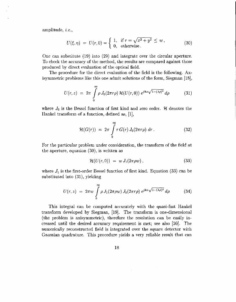
The procedure for the direct evaluation of the field is the following. Ax- isymmetric problems like this one admit solutions of the form, Siegman [18],

00

where JO is the Bessel function of first kind and zero order. X denotes the Hankel transform of a function, defined as, [l],

For the particular problem under consideration, the transform of the field at the aperture, equation (30), is written as

where J1 is the first-order Bessel function of first kind. Equation (33) can be substituted into (31), yielding

00

This integral can be computed accurately with the quasi-fast Hankel transform developed by Siegman, [19]. The transform is one-dimensional (the problem is axisymmetric) , therefore the resolution can be easily in- creased until the desired accuracy requirement is met; see also [20]. The numerically reconstructed field is integrated over the square detector with Gaussian quadrature. This procedure yields a very reliable result that can

18

be used as a reference to check the accuracy of the proposed method based on equation (29).

Results of numerical tests with parameters from cases A and B above are given below. The beam at the circular aperture has uniform intensity and phase. For the proposed method, 2048 x 2048 equispaced points were used in the integration over the aperture. On the other hand, the quasi-fast Hankel transform was performed on a grid of 32768 points, and the field was evaluated at 8192 x 8192 points inside the square detector.

These tests indicate that the accuracy of the proposed method is satis- factory. Figure 11 contains plot of the phase error in the phase for a beam coming off a circular element. The parameters of the problem were the same as in case A above. The error peak was just 4pm at x = 9 m . Figure 12 contains plot of the phase error when the parameters were chosen from case B. The error peak was 23.14pm at x = 12m. It is worth mentioning that the proposed algorithm is sufficiently fast. This is because it relies on simple solutions of the field which are computed very rapidly. Further, it is quite robust and powerful because equation (29) is exact; no approximations have been made for its derivation.

Conclusions

Fourier-based algorithms for computing the average phase of a beam over an element in the near field have been examined in the present study. Typi- cally, this is a two-step procedure. First, the field is computed numerically, and then it is integrated over the area of the element. For large Fresnel numbers (larger than about 20), the most accurate result can be obtained with the angular spectrum method. For smaller Fresnel numbers it can be obtained with direct evaluation of the Fresnel diffraction integral (11) via the Goertzel-Reinsch algorithm.

The numerical integration of the field can be best performed with Gaus- sian quadrature. However, the field is typically evaluated on equispaced grids and, therefore, gaussian quadrature can not be employed. Nonetheless, the two-dimensional version of Simpson’s rule provides sufficient accuracy. In all cases tested, the error in the average phase was smaller than 15 picometers if the appropriate algorithm was used.

Additionally, a new method to compute the average phase was introduced. It relies on a reciprocity property of the average phase and it requires the partioning of the optical element of interest to rectangles (for which closed-

19

form solutions of the field exist). Preliminary numerical tests showed that this method yields satisfactory results and, therefore, can be considered as a viable alternative to two-step procedures. Finally, for over-sized elements, analytical expressions for the average phase were presented that do not re- quire any numerical integration.

Acknowledgments

This work was prepared at the Jet Propulsion Laboratory, California Institute of Technology, under a contract with NASA. The authors would like to extend their thanks to Dr. R. Benson of Lockheed Martin Missiles and Space, for recommending the Goertzel-Reinsch algorithm and providing its subroutine. They would also like to thank Dr. M. Milman, Dr. M. Vaez- Iravani, and Dr. P. Dumont of JPL, for many fruitful discussions.

References

1. GOODMAN, J.W., Introduction to Fourier Optics, McGraw-Hill, (1996).

2. SAMNES, J.J., SPJELKAVIC, B., and PEDERSEN, H.M., “Evaluation of diffraction integrals using local phase and amplitude approxima- tions,” Opt. Acta, (1983), Vol. 30, pp. 207-222.

3. D’ARCIO, L.A., BRAAT, J. J.M., and FRANKENA, H. J., “Numerical evaluation of diffraction integrals for apertures of complicated shape,” J . Opt. SOC. Am. A, (1994), Vol. 11, pp. 2664-2674.

4. SOUTHWELL, W.H., ‘Validity of the Fresnel approximation in the near field,” J . Opt. SOC. Am., (1981), Vol. 71, pp. 7-14.

5 . KRAUS, H.G., “Finite element area and line integral transforms for generalization of aperture functions and geometry in Kirchhoff scalar diffraction theory,” Opt. Eng., (1993), Vol. 32, pp. 368-383.

6. HORWITZ, P., “Modes in missaligned unstable resonators,” Appl. Opt., (1976), Vol. 15, pp. 167-178.

7. CARCOLE, E., BOSCH, S., and CAMPOS, J., “Analytical and numer- ical approximations in Fresnel diffraction. Procedures based on the geometry of the Cornu Spiral.” J . Mod. Opt., (1993), Vol. 40, pp. 1091-1106.

20

8. SZICLAS, E., and SIEGMAN, A.E., “Mode calculations in unstable resonators with flowing saturable gain. 2: Fast Fourier Transform method,” Appl. Opt., (1975), Vol. 14, pp. 1874-1889.

9. MANSURIPUR, M., “Certain computational aspects of vector diffrac- tion problems,” J . Opt. Soc. Am. A, (1989), Vol. 6, pp. 786-805.

10. MENDLOVIC, D., ZALEVSKY, Z . , and KONFORTI, N., “Computation considerations and fast algorithms for calculating the diffraction inte- gral,” J . Mod. Opt., (1997), Vol. 44, pp. 407-414.

11. MAS, D., GARCIA, J., FERREIRA, C., BERNADO, L.M., and MAR- INHO, F., “Fast algorithms for free-space diffraction patterns calcula- tion,” Opt. Comm., (1999), Vol. 164, pp. 233-245.

12. STOER, J., and BULIRSCH, R., Introduction to Numerical Analysis, Springer-Verlag, (1 980).

13. CLENSHAW, C.W., and CURTIS, A.R., “A method for numerical in- tegration on an automatic computer,” Numerishe Mathematik, (1960), Vol. 2, pp. 197-205.

14. LITTLEWOOD, R.K., and ZAKIAN, V., “Numerical evaluation of Fourier integrals,” J . Inst. Math. Appl., (1976), Vol. 18, pp. 331-339.

15. LEVIN, D . , “Procedures for computing one- and two- dimensional in- tegrals of functions with rapid irregular oscillations,” Math. Comp., (1982), Vol. 38, pp. 531-538.

16. GRADSHTEYN, I.S., AND RYZHIK, I.M., Tables o fh tegral , series, and Products, Academic Press, (1992).

17. KRESS, R., Linear Integral Equations, Springer Verlag, (1989).

18. SIEGMAN, A.E., Lasers, University Science Books, (1977).

19. SIEGMAN, A.E., “Quasi-fast Hankel Transform,” Opt. Lett., (1977), Vol. 1, pp. 13-15.

20. VAEZ-IRAVANI, M., and WICKRAMASINGHE, H.K., “Scattering ma- trix approach of thermal wave propagation in layered structures,” J. A p ~ l . Ph., (1983), Vol. 58, pp. 122-132.

21

Figure Captions

Figure 1: Schematic of the test cases.

Figure 2: Case A.

Figure 3: Case A.

Figure 4: Case A.

Figure 5: Case B.

Figure 6: Case B.

Figure 7: Case B.

Figure 8: Case B.

Plot of the optical field at y = 0, z = 7 m.

Average-phase error of the angular spectrum method.

Average-phase error of the direct method.

Plot of the optical field at y = 0, x = 10 m.

Average-phase error of the angular spectrum method.

Average-phase error of the direct method.

Average-phase error of the two methods as a function of Fresnel number. x = 0.1, . . . ,2.2 m.

Figure 9: Case C. Plot of the optical field at y = 0, z = 10 m.

Figure 10: Case C. Average-phase error of the angular spectrum method.

Figure 11: Case C. Average-phase error of the direct method.

Figure 11: Case C. Numerical convergence of the two methods. N is the number of grid points at each direction, in the aperture plane. x = 11.65 m.

Figure 13: Case A; circular aperture, diameter 3 cm. Average-phase error of the proposed alternative method.

Figure 14: Case B; circular aperture, diameter 5 mm. Average-phase error of the proposed alternative method.

22

23

1.4 I I I I I I I

1.2

0 -

- 0.2

- 0.4

- E 0.6

- 5 0.8

1 -

- -

-

>.

c -

a - - -

-

I I I I I

-3 -2 -1 0 1 2 3 x (cm)

-4 ' I I I I I I -3 -2 -1 0 1 2 3

x (cm)

24

15

10

5

h

v k g o ti L

E

-5

-1 c

-1 E

ANGULAR SPECTRUM METHOD I I I I I I I I

A

A

I

A . . . .

A

A

A

A

A :' 'A

A

A

a

A

h A Y . .

h

d

.. A

A

A

A

A

A, : 'A

A . . . . : A

A 1,

A

4

A

A

5 I I I I I I I I I

7.2 7.4 7.6 7.8 8 8.2 8.4 8.6 8.8 9 I

(m)

25

26

I I I I I I I

-20 -1 5 -1 0 -5 0 5 10 15 20 x (mm)

27

800

600

400

h

v k L

2 & 200 8 m .K Q

0

-200

ANGULAR SPECTRUM METHOD I I I I I I I I I

A

A A

. . _ .

. .

A A A

A , ,' A

. . . . . . . .

A : . .

. .

A I I I I I I I I I

28

DIRECT METHOD 0.5

0.45

0.4

0.35 h

v E

8

L

2 $ 0.3

.c a. 0.25

0.2

0.1 5

I I I I I

A A'

A ' A'

A ' A

n A

A A'

n a

A

A

A

A

I -

I -

-

I -

-

-

1 -

. .

0.1 I I I I I I I I I 1 10 10.2 10.4 10.6 10.8 1 1 1 1.2 11.4 11.6 11.8 12

(m)

29

Fresnel number

DIRECT METHOD 300 I I I t I

h 2oo[ 5 100

0 10 20 30 40 50 60 Fresnel number

30

1.4

1.2

1

p0 .8

E 0.6

0.4

0.2

0

c a -

-3 -2 -1 0 1 2 3 x (cm)

" " I -4 ' I 1 1 1 1 1

-3 -2 -1 0 1 2 3 x (cm)

31

32

DIRECT METHOD 10 I I I I I I I I I

a 8 -

A . . . . A

: : A A 6 - :. . .

. .

. . . .

. . . . . . . . . . . . . .

4 - : : : : . . . . . . . . . . : . A 4 a

. . . .

. .

. . . .

. . . .

. . . . A _ . A . . ' A : : - A : : : : ; ,

. . . . . . .

. . . .

. . . . . . . 2 - : 1 : : . . . . . . . . . . . . . . . . . . . . . . . . .

. . . . . . . . . .

E

D

. . . . . . . . . . . . . . . . . . . . . . . .

Y L

2 5 O - : A : : :

. . . . A : . . . . . .

. . . . . .

. . . . . . . . . . . . . . . . . . . . . . . . . . . . . . . . .

. . . . . . . . . . . . . . . .

. . . . . . . .

. . . . . .

c . . . .

- 2 - . . . . . . . . . . . .

. . . . . . . .

. . . . . . . .

-4 - : A A A L I A

'4 . . A A : ; . . . . . h ' : : ;

: ' . A '.

: A . ;

. . . . . . . . . .

.' A . . . .

. . . . . . . . . .

. . . . , . . .

. . . . _ .

. . . . . . . . A _ . . . _ . . .

A d A

33

200

150 h

E v b

Q

100 a, a v)

r 0-

50

ANGULAR SPECTRUM METHOD I 1 . . . . . . . . . . . , . . _ . I . . .

' ' " . . . . A .

DIRECT METHOD 1000 I I I I I

800 - -

h

E A , . , .

600 - I .

( . ' .A

2 % 2 400

-

-

a,

c -

a

200 - -

O5 I I I m I

6 7 8 9 10 1 1 -

log2(N)

34

PROPOSED ALTERNATIVE METHOD

35

36