Business cycles, monetary transmission and shocks to ... · BUSINESS CYCLES, MONETARY ... Based on a range of quarterly business cycle indicators this paper ... quarterly national

WORKING PAPER SERIESNO 1458 / AUGUST 2012

BUSINESS CYCLES, MONETARYTRANSMISSION AND SHOCKS

TO FINANCIAL STABILITY

EMPIRICAL EVIDENCE FROM A NEW SET OF DANISH QUARTERLY NATIONAL ACCOUNTS 1948-2010

Kim Abildgren

NOTE: This Working Paper should not be reported as representing the views of the European Central Bank (ECB). The views expressed are

those of the authors and do not necessarily reflect those of the ECB.

MACROPRUDENTIAL RESEARCH NETWORK

© European Central Bank, 2012

AddressKaiserstrasse 29, 60311 Frankfurt am Main, Germany

Postal addressPostfach 16 03 19, 60066 Frankfurt am Main, Germany

Telephone+49 69 1344 0

Internethttp://www.ecb.europa.eu

Fax+49 69 1344 6000

All rights reserved.

ISSN 1725-2806 (online)

Any reproduction, publication and reprint in the form of a different publication, whether printed or produced electronically, in whole or in part, is permitted only with the explicit written authorisation of the ECB or the authors.

This paper can be downloaded without charge from http://www.ecb.europa.eu or from the Social Science Research Network electronic library at http://ssrn.com/abstract_id=2128479.

Information on all of the papers published in the ECB Working Paper Series can be found on the ECB’s website, http://www.ecb.europa.eu/pub/scientific/wps/date/html/index.en.html

Macroprudential Research NetworkThis paper presents research conducted within the Macroprudential Research Network (MaRs). The network is composed of econo-mists from the European System of Central Banks (ESCB), i.e. the 27 national central banks of the European Union (EU) and the Euro-pean Central Bank. The objective of MaRs is to develop core conceptual frameworks, models and/or tools supporting macro-prudential supervision in the EU.

The research is carried out in three work streams:1) Macro-financialmodelslinkingfinancialstabilityandtheperformanceoftheeconomy;2) Earlywarningsystemsandsystemicriskindicators;3) Assessing contagion risks.

MaRs is chaired by Philipp Hartmann (ECB). Paolo Angelini (Banca d’Italia), Laurent Clerc (Banque de France), Carsten Detken (ECB), Cornelia Holthausen (ECB) and Katerina Šmídková (Czech National Bank) are workstream coordinators. Xavier Freixas (Universitat Pompeu Fabra) and Hans Degryse (Katholieke Universiteit Leuven and Tilburg University) act as external consultant. Angela Maddaloni (ECB) and Kalin Nikolov (ECB) share responsibility for the MaRs Secretariat. The refereeing process of this paper has been coordinated by a team composed of Cornelia Holthausen, Kalin Nikolov and Bernd Schwaab (all ECB). The paper is released in order to make the research of MaRs generally available, in preliminary form, to encourage comments and sug-gestionspriortofinalpublication.Theviewsexpressedinthepaperaretheonesoftheauthor(s)anddonotnecessarilyreflectthoseof the ECB or of the ESCB.

AcknowledgementsThe author wishes to thank colleagues from Danmarks Nationalbank for useful comments on preliminary versions of this paper. The author alone is responsible for any remaining errors. The content of this Working Paper was presented at the 1st Conference of the European System of Central Banks Macro-Prudential Research (MaRs) Network held at the premises of the European Central Bank, Frankfurt, 5-6 October 2011. A journal article based on the work in the paper was recently published (cf. Abildgren, Kim, Business Cycles and Shocks to Financial Stability - Empirical evidence from a new set of Danish quarterly national accounts 1948-2010, Scan-dinavian Economic History Review, Vol. 60(1), 2012, pp. 50-78). Views and conclusions expressed in the paper are those of the author and do not necessarily represent those of Danmarks Nationalbank.

Kim AbildgrenatDanmarksNationalbank,Havnegade5,DK-1093CopenhagenK,Denmark;e-mail:[email protected]

Abstract

In Denmark official quarterly national accounts are only available for the period since 1977.

The paper constructs a set of summary non-seasonally adjusted quarterly national accounts

for Denmark for 1948-2010 in current and constant prices as well as a set of other key

quarterly macroeconomic indicators covering the Danish economy since 1948. As a first

exploratory analysis of these two new data sets the paper reviews some of the stylised

empirical evidence on the business cycle, the monetary transmission mechanism and shocks

to financial stability that can be uncovered using filtering techniques and reduced-form vector

autoregressive (VAR) models. The long-span data sets make it possible to estimate VAR

models of a higher dimension than is usually found in the literature due to degrees-of-freedom

problems. The results from the VAR analysis indicate a significant and long-lasting negative

impact on real GDP following an exogenous shock to the banking sector’s write-down ratio.

Key words: Quarterly national accounts; Danish economic history; business cycles; monetary

transmission; financial stability; band-pass filters; VAR analysis.

JEL Classification: C32; C82; E01; E32; E44; E52; N14.

Resumé (Danish summary)

I Danmark foreligger kun officielle kvartalsvise nationalregnskaber for perioden siden 1977. I

papiret konstrueres et sæt summariske ikke-sæsonkorrigerede kvartalsvise nationalregnskaber

for Danmark i såvel løbende som faste priser for perioden 1948-2010. Endvidere konstrueres

et supplerende datasæt, som indeholder en række øvrige kvartalsvise makroøkonomiske

indikatorer for den danske økonomi dækkende samme periode. Som en første eksplorativ

analyse af disse to nye datasæt gennemgås de empiriske stiliserede fakta omkring

konjunkturcykler, den pengepolitiske transmissionsmekanisme og finansiel stabilitet, som kan

udledes på basis af filtreringsteknikker og vektorautoregressive (VAR) modeller. De nye

lange tidsserier gør det muligt at estimere VAR modeller af en højere dimension, end der

normalt ses i litteraturen som følge af problemer med manglende frihedsgrader. VAR

analyserne indikerer, at der kan være en signifikant og langvarig negativ påvirkning af det

reale bruttonationalprodukt efter et eksogent stød til bankernes nedskrivningsprocenter.

1

Non-technical summary In Denmark official time series of quarterly national accounts are only available for the period since

1977. Based on a range of quarterly business cycle indicators this paper constructs a set of summary

non-seasonally adjusted quarterly national accounts for Denmark 1948-2010 in current and constant

prices as well as a set of other key quarterly macroeconomic indicators covering the Danish

economy since 1948. Based on these new data sets the paper reviews the empirical evidence on

shocks to financial stability and the linkages between the financial sector and the real economy in

the Danish post-war period that can be uncovered using structural vector autoregressive (VAR)

models.

VAR models have found extensive use in relation to studies on monetary transmission and have

more recently also found use in relation to studies on the robustness of the banking system to

adverse macroeconomic shocks and on the feedback effects on the macroeconomy of shocks to

financial stability. The new long-span data sets presented in the paper make it possible to estimate

VAR models of higher dimensions than usually found in studies covering not only Denmark but

also many other countries due to lack of degrees of freedom.

The standard VAR model used in the literature for analysing monetary transmission usually

includes three endogenous variables: Real GDP, CPI, and the short-term interest rate. In addition to

these three variables the VAR models estimated in this paper includes six more endogenous

variables commonly known to be of interest in relation to financial stability. The additional six

variables are the yield on long-term central-government bonds, share prices, broad money, domestic

credit, house prices and the banks’ write-down ratio (i.e. loan impairment charges in per cent of

loans and guarantees).

In the VAR models the banks’ write-down ratio is used as an indicator of the robustness of the

banking sector, and widespread financial instability can be represented in the model via an

exogenous shock to the banks’ write-down ratio. Such a shock might be interpreted as a financial

stability shock originating from within the banking sector, for instance a sudden reassessment of the

credit quality of the banks’ loan portfolio or a sudden extraordinarily increase in the banking

sectors’ risk aversion. However, the model allows for other interpretations as well. An

extraordinarily large increase in the banking sector’s write-down ratio could for instance reflect

weakened confidence in the banking sector, which increases the saving behaviour of households

and firms and generates a deep recession. The banks’ write-downs express the banks’ expected

2

future losses and historically write-downs have been booked 1-2 years before the losses are realised.

The banks’ write-down ratio is therefore also a useful indicator of current systemic stress or

instability.

The results of the VAR analysis in the paper indicate that an exogenous increase in the banking

sector’s write-down ratio is related to a significant and long-lasting decline in domestic credit,

house prices and real GDP. This finding is consistent with recent economic-historical research,

which indicates that the economic recovery after a banking crisis tends to be slower than normal.

The VAR model estimated in the paper has found use as a tool to quantify the real effects of

banking crises in Danish post-World War II economic history, cf. Abildgren, Kim, Birgitte Vølund

Buchholst, Atef Qureshi and Jonas Staghøj, Real Economic Consequences of Financial Crises,

Danmarks Nationalbank Monetary Review, Vol. 50(3:2), 2011, pp. 1-49. In this study the authors

estimated the development in real GDP five years ahead, corresponding to the extraordinary

increases in the Danish banking sector’s write-downs in 1991-93 and 2008. The extraordinary

increase in the banks’ write-downs in 2008 was equivalent to real GDP in the 1st half of 2010 being

around 3 per cent lower than in a baseline scenario without a financial crisis. Similarly, the

extraordinary increases in the banking sector’s write-downs in 1991-93 became – over a few years –

equivalent to a level of real GDP that was around 3 per cent lower than in the baseline scenario.

3

1. Introduction

In the wake of the international financial crisis 2008/2009, the interactions between the

banking system and the macro economy have once again been among the issues at the top of

the research agenda. A deeper empirical understanding of these issues requires a careful

analysis of the rich and complicated dynamic interactions between a range of macroeconomic

variables and could therefore benefit from access to long-span consistent time series of

national accounts and other key macroeconomic indicators at a quarterly frequency.

Unfortunately, researchers often have to rely on either long annual time series or quarterly

data covering only the most recent decades.

The expansion of the official statistics with quarterly national accounts occurred rather late

in Denmark compared to other countries. In the USA quarterly national accounts were

introduced already in the 1940s, UK and Canada followed in the 1950s and Sweden and

Finland in the 1960s. Statistics Denmark – the central bureau of statistics in Denmark – only

introduced quarterly national accounts for Denmark in 1988 and the first release covered just

6 quarters of data (Berner & Thage, 1989; Graversen et al., 2008). At a later stage Statistics

Denmark released series back to 1977 (Sørensen, 1994a, 1994b, 1994c).

No official quarterly national accounts are available for Denmark prior to 1977. For

selected pre-1977 periods other authors have previously published quarterly national-account

data for Denmark following different compilation methods. However, the lack of a consistent

set of long-span quarterly national-account aggregates prior to 1977 limits the scope for

business cycle analysis and short-term dynamic modelling of the Danish economy.

The paper at hand presents and documents a set of summary non-seasonally adjusted

quarterly national accounts for Denmark in current and constant prices for the period since

1948. The data set contains a breakdown of GDP into private consumption, government

consumption, gross investments, exports of goods and services and imports of goods and

services. In order to facilitate the analytical application of the new historical quarterly

national-account data, the author has also compiled a collection of seventeen other key

quarterly macroeconomic indicators for the Danish economy covering the period since 1948.

Furthermore, as a first exploratory analysis of these two new data sets the paper reviews

some of the stylised empirical evidence on the business cycle, monetary transmission and

financial stability that can be uncovered from the data using filtering techniques and reduced-

form VAR models. The two new long-span data sets make it possible to estimate VAR

models of higher dimensions than usually found in studies covering not only Denmark but

also many other countries due to lack of degrees of freedom. The VAR models presented in

this paper contain nine endogenous variables. They are therefore able to add new empirical

evidence on the influence of macroeconomic shocks on the banking sectors’ write down ratio.

4

Furthermore, the models can also throw some new light on the output effects of shocks to

financial stability.

2. Previous works on pre-1977 quarterly national accounts in Denmark

Danmarks Nationalbank – the central bank of Denmark – has compiled a rather detailed set of

quarterly national-account statistics for the period since 1971 in relation to the construction of

a macroeconometric model for Denmark (Christensen, 1989; Christensen & Knudsen, 1992;

Danmarks Nationalbank, 2003). The work on quarterly national accounts at the Nationalbank

is still going on. Each quarter the Nationalbank converts a large number of short-term

business cycle indicators into a set of quarterly national-account figures in order to have a

comprehensive and consistent picture of the latest economic development prior to the release

of the official quarterly national-account data from Statistics Denmark.

Thygesen (1971) presents estimates of quarterly GDP in current prices 1951-1968 in

relation to an econometric study on monetary transmission in Denmark. These GDP estimates

are based on only three business cycle indicators (retail sales, exports and constructions

started in a quarter).

Hansen & Paldam (1973) document a more detailed set of quarterly national-account

indicators that served as the basis for a macroeconometric model at the Danish Council of

Economic Advisors. However, the longest time series in the data set covers only the period

1960-1969, and many of the time series are even shorter. Furthermore, the data set is not

tabulated in Hansen & Paldam, op.cit., and is not available in the archives of the Danish

Council of Economic Advisors.

3. Summary quarterly national accounts for Denmark 1948-2010 - compilation

approach

In the quarterly national accounts 1948-2010 presented in this paper GDP is broken down into

the following five expenditure items:

[E.1] Private consumption [E.2] Government consumption [E.3] Gross investments [E.4] Exports of goods and services [E.5] Imports of goods and services

The data set consists of non-seasonally adjusted data in current and constant prices. The

description of data sources and compilation methods applied for the construction of the data

set can be divided into three parts covering respectively the periods 1948-1971, 1971-1977,

and 1977-2010. The series for the three sub-periods were subsequently chained together to the

overall series.

5

Compilation approach 1977-2010

For the period 1977-2010 the data set builds directly on the non-seasonally adjusted quarterly

national account data in current and constant prices published by Statistics Denmark.

Adjustments have been made for breaks in the series in 1988 and 1990.


Danmarks Nationalbank has compiled seasonally adjusted data in current and constant prices

covering the period 1971-1977. These series were converted into non-seasonally adjusted data

using seasonal factors from 19772 based on the quarterly national accounts from Statistics

Denmark.


The compilation approach for the pre-1971 period has to a high degree been determined by

data availability. An important design criterion was to be able to base the quarterly national

accounts series on a fairly consistent set of key business cycle indicators published on a

quarterly basis without (or nearly without) gaps.

For the pre-1971 calculations the five expenditure items of GDP were disaggregated further

into a total of twelve expenditure items, cf. Table 1.

Table 1: Quarterly indicators used in the compilation procedure 1948-1971 Quarterly indicator National accounts expenditure

component [a] Current prices [b] Constant prices [c] Price index [E.1a] Retail goods Value index for retail sales Accounting identity (a/c) Consumer price index

[E.1b] Purchase of vehicles

Accounting identity (b*c) Number of new registrations of personal vehicles

Consumer price index

[E.1] Private consumption

[E.1c] Other private consumption

NO INDICATOR NO INDICATOR NO INDICATOR

[E.2] Government consumption NO INDICATOR NO INDICATOR NO INDICATOR [E.3a] New construction of residential buildings

Accounting identity (b*c) Number of dwellings started (lagged 1 quarter)

Index for building costs

[E.3b] New construction of other buildings and civil engineering works

Accounting identity (b*c) Gross floor space (m2) of new buildings started excluding dwellings started (lagged 1 quarter)

Index for building costs

[E.3c] Other gross fixed business investments

Accounting identity (b*c) Number of new registrations of commercial vehicles

Wholesale price index

[E.3] Gross investments

[E.3d] Changes in inventories

NO INDICATOR NO INDICATOR NO INDICATOR

[E.4a] Goods Value of exports of goods Accounting identity (a/c) Export unit values for goods

[E.4] Exports of goods and services [E.4b] Services Value of exports of

services Accounting identity (a/c) Export unit values for

goods [E.5a] Goods Value of imports of goods Accounting identity (a/c) Import unit values for

goods [E.5] Imports of goods and services [E.5b] Services Value of imports of

services Accounting identity (a/c) Import unit values for

goods

2 The seasonal factors for 1977 and the nearest following years in the quarterly national accounts from Statistics Denmark are relatively stable.

6

For nine of the twelve expenditure items ([E.1a], [E.1b], [E.3a], [E.3b], [E.3c], [E.4a],

[E.4b], [E.5a] and [E.5b]) the quarterly national-account data were compiled via a two-step

procedure: In step 1 a quarterly indicator in both current as well as constant prices was

constructed for each of the nine expenditure components, cf. Table 1. In step 2 figures for the

nine expenditure components in current and constant prices from the annual national-account

statistics released by Statistics Denmark for the years 1948-1971 were interpolated on

quarters utilising the indicators constructed in step 1 as distributions keys.

One simple approach would have been to distribute the observations from the annual

national-account statistics proportionally over the four quarters of the year using the quarterly

indicator series as distribution keys. However, such a procedure would lead to discontinuities

around each year turn in the quarterly national-account series (in the literature known as the

“step problem”). The technique used for the interpolation in step 2 was therefore based on the

so-called “Proportional Denton Least Square Method”, cf. Denton (1971).3 This method

minimises the least-squares differences in the quarter-on-quarter development in the ratio

between the quarterly interpolated national-account series and the quarterly indicator series

subject to the constraint that the sum of the quarterly interpolated national-account series over

the four quarter within a year should be equal to the annual national-account figure.

Mathematically the Proportional Denton Method can be formulated as follows:

[ ] ∑ ==∑

−

−==−

−4y

34yt

y

t

2

T

2t1t

1t

t

t

)QNAT,...,(QNA1

A,...1,y,ANAQNAtosubjectI

QNA

I

QNAminimise1

where:

QNAt = the observation in quarter t in the interpolated quarterly national account series. ANAy = the observation in year y in the annual national account series. It = the observation in quarter t in the quarterly indicator series. T = the last quarter for which the quarterly indicator series is available and the last

quarter for which the quarterly national account series is to be interpolated. A = the last year for which the annual national account series is available.

As shown in Table 1 no indicator series were available for three of the twelve expenditure

components ([E.1c], [E.2] and [E.3d]). For these components the quarterly national account

series had to be based solely on the annual national account statistics in current and constant

prices. The quarterly national-account data for these three items were therefore constructed

3 The Proportional Denton Least Square Method is recommended as the preferred method to compile quarterly national-account data on the basis of annual national accounts and a quarterly indicator series in the IMF manual on quarterly national accounts, cf. chapter 6 in Bloem et al. (2001).

7

using the mechanical least-squares-based technique described in Boot et al. (1967).4 This

method - which ensures a smooth quarterly interpolated national-account series - minimises

the squared first differences of the quarterly interpolated national-account series subject to the

constraint that the sum over the four quarters within a year is equal to the correspondent

annual national-account figure. The method can be formulated as follows:

[ ] ( ) ∑ ==∑ −−==

−

4y

34yt

y

t

2T

2t 1tt)QNAT

,...,QNA1(

A,...1,y,ANAQNAtosubjectQNAQNAminimise2

where:

QNAt = the observation in quarter t in the interpolated quarterly national account series. ANAy = the observation in year y in the annual national account series. T = the last quarter for which the quarterly national account series is to be

interpolated. A = the last year for which the annual national account series is available.

A first look on the data set

Annex A contains a more detailed documentation of the data sources used to construct the

quarterly national accounts 1948-2010 whereas annex B lists the data set. This data set is also

available in electronic form on request from the author.

Nominal and real year-on-year growth rates of the quarterly national-account aggregates are

shown in Chart 1-7. These charts put the recent great recession in a clear historical

perspective. Measured by real GDP year-on-year growth rates the recession in 2008/2009

following the international financial crisis has been the deepest downturn in the post–1948

period, cf. Chart 7. This recession in 2008/2009 was mainly characterised by significant drops

in the private consumption and in the exports of goods and services, cf. Chart 1 and 5. The

decline in total domestic demand in 2008/2009 was by and large at the same level as the

decline experienced following the first and second oil-price shocks in the 1970s and early

1980s, cf. Chart 4.

4 The least-squares technique presented in Boot et al. (1967) is one of the methods recommended in the IMF manual on quarterly national accounts when one has to compile quarterly national-account data on the basis of annual national accounts and no relevant quarterly indicators are available, cf. chapter 7 in Bloem et al. (2001). In case of gross investment in stock building the procedure in Boot et al. (1967) was only applied to the figures in current prices. Here the quarterly figures in constant prices were calculated on the basis of the figures in current prices deflated by the consumer price index. It would have been possible to incorporate seasonal variation into the quarterly interpolated national-account series for [E.1c] Other private consumption and [E.2] Government consumption based on seasonal factors from the year 1977 in Statistics Denmark’s quarterly national-account statistics. However, there is almost no seasonal pattern in these two series.

8

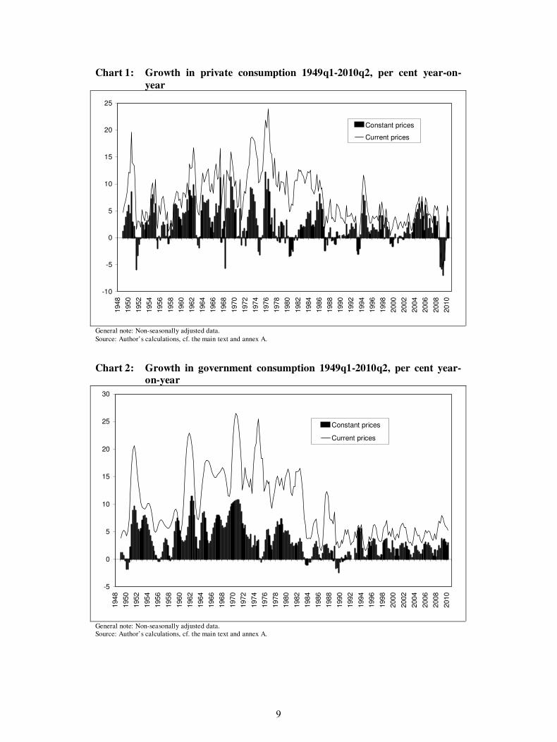
Chart 1: Growth in private consumption 1949q1-2010q2, per cent year-on-

year

-10

-5

0

5

10

15

20

25

1948

1950

1952

1954

1956

1958

1960

1962

1964

1966

1968

1970

1972

1974

1976

1978

1980

1982

1984

1986

1988

1990

1992

1994

1996

1998

2000

2002

2004

2006

2008

2010

Constant prices

Current prices

General note: Non-seasonally adjusted data. Source: Author’s calculations, cf. the main text and annex A.

Chart 2: Growth in government consumption 1949q1-2010q2, per cent year-on-year

-5

0

5

10

15

20

25

30

1948

1950

1952

1954

1956

1958

1960

1962

1964

1966

1968

1970

1972

1974

1976

1978

1980

1982

1984

1986

1988

1990

1992

1994

1996

1998

2000

2002

2004

2006

2008

2010

Constant prices

Current prices


9

Chart 3: Growth in gross investments 1949q1-2010q2, per cent year-on-year

-40

-30

-20

-10

0

10

20

30

40

50

60

1948

1950

1952

1954

1956

1958

1960

1962

1964

1966

1968

1970

1972

1974

1976

1978

1980

1982

1984

1986

1988

1990

1992

1994

1996

1998

2000

2002

2004

2006

2008

2010

Constant prices

Current prices


Chart 4: Growth in total domestic demand 1949q1-2010q2, per cent year-on-

year

-10

-5

0

5

10

15

20

25

30

1948

1950

1952

1954

1956

1958

1960

1962

1964

1966

1968

1970

1972

1974

1976

1978

1980

1982

1984

1986

1988

1990

1992

1994

1996

1998

2000

2002

2004

2006

2008

2010

Constant prices

Current prices


10

Chart 5: Growth in exports of goods and services 1949q1-2010q2, per cent

year-on-year

-30

-20

-10

0

10

20

30

40

50

1948

1950

1952

1954

1956

1958

1960

1962

1964

1966

1968

1970

1972

1974

1976

1978

1980

1982

1984

1986

1988

1990

1992

1994

1996

1998

2000

2002

2004

2006

2008

2010

Constant prices

Current prices


Chart 6: Growth in imports of goods and services 1949q1-2010q2, per cent year-on-year

-30

-20

-10

0

10

20

30

40

50

60

1948

1950

1952

1954

1956

1958

1960

1962

1964

1966

1968

1970

1972

1974

1976

1978

1980

1982

1984

1986

1988

1990

1992

1994

1996

1998

2000

2002

2004

2006

2008

2010

Constant prices

Current prices


11

Chart 7: Growth in gross domestic product 1949q1-2010q2, per cent year-on-

year

-10

-5

0

5

10

15

20

25

1948

1950

1952

1954

1956

1958

1960

1962

1964

1966

1968

1970

1972

1974

1976

1978

1980

1982

1984

1986

1988

1990

1992

1994

1996

1998

2000

2002

2004

2006

2008

2010

Constant prices

Current prices


During the 1930s and the World War II the international economy had developed into a

system characterised by a complex net of bilateral clearing and payment arrangements. The

very high growth rates of imports and exports during the late 1940s and early 1950s, cf. Chart

5 and 6, reflect the deregulation of quantitative trade restrictions within the framework of the

Organisation for European Economic Co-operation (OEEC). The process was facilitated by

the Marshall Aid 1948-1953 and the establishment of the European Payment Union (EPU) in

1950 which ensured a high degree of de facto internal current-account convertibility among

the participating European currencies – including Danish kroner – through a monthly

multilateral clearing system for current payments, cf. Mikkelsen (1999). The export and

import ratios for the Danish economy increased from around 20-25 per cent of GDP in 1948

to around 35-40 per cent in the early 1950s, cf. Chart 8.

12

Chart 8: Exports and imports of goods and services in current prices 1948q1-

2010q2, per cent of GDP

15

20

25

30

35

40

45

50

55

60

19

48

19

50

19

52

19

54

19

56

19

58

19

60

19

62

19

64

19

66

19

68

19

70

19

72

19

74

19

76

19

78

19

80

19

82

19

84

19

86

19

88

19

90

19

92

19

94

19

96

19

98

20

00

20

02

20

04

20

06

20

08

20

10

Exports

Imports


The growth pattern of the Danish economy during the 1950s, cf. Chart 7, reflects the stop-

go policy adopted during this period in order to trade-off the desire for full employment and

the need to keep the balance of payments close to zero. At the end of the 1950s the scope for

Danish foreign borrowing improved significantly and the 1960s and early 1970s were most of

the period characterised by solid growth. The 1960s also saw the build up of a large tax-

financed welfare state, which is reflected in the substantial real growth rates in government

consumption, cf. Chart 2. The expansion of the domestic economy during the 1960s resulted

in a significant deficit on the trade balance, cf. Chart 9. The negative growth rate in real GDP

in 1963 in Chart 7 reflects a tightening of economic policies with the introduction of a general

sales tax in 1962 and a number of income policy measures (“the package solution”) in 1963 in

order to address the weakening of the trade balance. The negative growth rate in real GDP in

the first half of 1966 also reflects a tightening of economic policies (the general sales tax was

increased in 1965) combined with a long winter in 1965/1966.

13

Chart 9: Net exports of goods and services in current prices 1948q1-2010q2,

per cent of GDP

-10

-8

-6

-4

-2

0

2

4

6

8

10

1948

1950

1952

1954

1956

1958

1960

1962

1964

1966

1968

1970

1972

1974

1976

1978

1980

1982

1984

1986

1988

1990

1992

1994

1996

1998

2000

2002

2004

2006

2008

2010


A more detailed description of the economic development in Denmark 1948-1971 is found

in Johansen (1987); Hansen et al. (1988); Pedersen, P. J. (1996) and Økonomiministeriet

(1997). The period since 1971 is e.g. covered by Danmarks Nationalbank (2003) and

Johansen & Trier (2010). Some of the stylised facts and empirical regularities of the post-

1948 Danish business cycles will be further reviewed in section 5 below.

As a robustness check on the pre-1971 data construction Chart 10 and 11 compare the

development in the series for the nominal gross domestic product 1951-1968 constructed in

the paper at hand with the series presented in Thygesen (1971). Taking into account that the

two data series are based on rather different data sources and compilation procedures the two

series seem in broad terms to paint the same picture of the economic development in

Denmark 1951-1968.5

5 The correlation coefficient between the to series in Chart 10 (11) is 1.00 (0.62).

14

Chart 10: Gross domestic product, current prices 1951q1-1968q4, million

kroner

0

5000

10000

15000

20000

25000

30000

1951

1952

1953

1954

1955

1956

1957

1958

1959

1960

1961

1962

1963

1964

1965

1966

1967

1968

This study

Thygesen (1971)

General note: Non-seasonally adjusted data. Source: Annex B and Thygesen (1971).

Chart 11: Year-on-year growth in gross domestic product, current prices 1952q1-1968q4, per cent

-2

0

2

4

6

8

10

12

14

16

18

20

1952

1953

1954

1955

1956

1957

1958

1959

1960

1961

1962

1963

1964

1965

1966

1967

1968

This study

Thygesen (1971)

General note: Non-seasonally adjusted data. Source: Annex B and Thygesen (1971).

15

4. A supplementary data set on key quarterly macroeconomic indicators 1948-

2010

In order to enhance the analytical application of the new historical quarterly national-account

data the author also compiled a collection of seventeen other non-seasonally key quarterly

economic indicators for the Danish economy covering the period 1948-2010, cf. Table 2.

Table 2: Key quarterly macroeconomic indicators 1948-2010 Indicator Notes [I.1] Unemployment rate Unemployed persons in per cent of the total labour force. Quarterly

averages. [I.2] Index of average hourly earnings in manufacturing industries

Quarterly averages.

[I.3] Official discount rate of Danmarks Nationalbank

Quarterly averages.

[I.4] Yield on long-term Danish government bonds

Quarterly averages.

[I.5] Private banks’ average lending rate Weighted average lending interest rate of savings banks and commercial banks.

[I.6] Private banks’ average deposit rate Weighted average deposit interest rate of savings banks and commercial banks.

[I.7] Nominal effective krone-rate index Trade-weighted average of the development in the bilateral nominal krone-rate vis-à-vis the currencies of a range of Denmark’s main trading partners. An increase in the index describes an overall nominal appreciation of the Danish krone vis-à-vis the currencies of Denmark’s main trading partners. Quarterly averages.

[I.8] Consumer price index, Denmark Quarterly averages. [I.9] Consumer price index, abroad Trade-weighted average of the consumer price development in Denmark’s

main trading partners. Quarterly averages. [I.10] Real effective krone-rate index with consumer prices as deflator

Trade-weighted average of the development in the bilateral real krone-rate vis-à-vis the currencies of a range of Denmark’s main trading partners. CPIs are used as deflators. An increase in the index describes an overall real appreciation of the Danish krone vis-à-vis the currencies of Denmark’s main trading partners. Quarterly averages.

[I.11] Price index for sale of one-family houses Quarterly averages. [I.12] Share price index End of quarter. [I.13] Broad money stock (M2) End of quarter. [I.14] Credit to the domestic non-bank sector extended by resident commercial banks and savings banks

End of quarter.

[I.15] Credit to the domestic non-bank sector extended by resident mortgage banks

End of quarter.

[I.16] Credit to the domestic non-bank sector extended by all resident banks

[I.16] = [I.14] + [I.15]. End of quarter.

[I.17] Bank’s write-downs ratio Quarterly write-downs on loans and guaranties in per cent of end-quarter outstanding loans and guaranties. The write-down ratio is not annualised and covers write-downs in commercial banks and savings banks only.

A number of adjustments have been made in order to transform the background data into a

set of reasonable consistent set of economic indicators. Furthermore, it should be mentioned

that most of the quarterly data on bank’s write-down ratio have been interpolated from semi-

annual or annual data. It should also be noted, that for long periods the discount rate has not

been directly related to any of Danmark Nationalbank’s monetary-policy instruments.

However, for most of the post-1948 period the discount rate has served as a signal rate

indicating the general level of monetary-policy interest rates in Denmark.

The supplementary data set on key quarterly macroeconomic indicators 1948-2010 is shown

in Chart 12-19. During the solid growth in the Danish economy in the 1960s and early 1970s

the unemployment rate was at a very low level, cf. Chart 12. The seasonal volatility in the

16

unemployment figures seems to be relatively high in the period until the early 1970s

compared to the post-1970 period. This might be related to data issues but could also reflect

improved utilisation of the work force over the seasons during the last four decades, i.e.

within the building sector (pre-cast building).

The macroeconomic performance of the Danish economy deteriorated significantly during

the 1970s, particularly in the second half of the decade. The oil price shocks of the 1970s and

the devaluations of the krone caused a continuous upward pressure on price and wage

inflation and on nominal interest rates, cf. Chart 13 and 15. Furthermore, unemployment

increased rapidly. Due to worse inflationary performance than its main trading partners

Denmark experienced a marked appreciation of the real effective exchange rate from the late

1940s to the late 1970s, cf. Chart 14.

The post-1980 period witnessed significant improvements in the macroeconomic

performance of the Danish economy. Consumer price inflation declined from two digit-

figures in the early 1980s to a level around 2 per cent in the early 1990s. The unemployment

rate stayed at a high level until the middle of the 1990s but has since declined significantly.

Chart 12: Unemployment rate 1948q1-2010q2, per cent of the labour force

0

2

4

6

8

10

12

14

1948

1950

1952

1954

1956

1958

1960

1962

1964

1966

1968

1970

1972

1974

1976

1978

1980

1982

1984

1986

1988

1990

1992

1994

1996

1998

2000

2002

2004

2006

2008

2010

General notes: Non-seasonally adjusted data. Source: Author’s calculations, cf. the main text and annex A.

17

Chart 13: Interest rates 1948q1-2010q2, per cent per annum

0

2

4

6

8

10

12

14

16

18

20

22

24

26

1948

1950

1952

1954

1956

1958

1960

1962

1964

1966

1968

1970

1972

1974

1976

1978

1980

1982

1984

1986

1988

1990

1992

1994

1996

1998

2000

2002

2004

2006

2008

2010

Official discount rate of the Nationalbank

Yield on long-term government bonds

Banks’ average lending rate

Banks’ average deposit rate


Chart 14: Effective exchange rates 1948q1-2010q2, 1980=100

70

75

80

85

90

95

100

105

110

115

120

1948

1950

1952

1954

1956

1958

1960

1962

1964

1966

1968

1970

1972

1974

1976

1978

1980

1982

1984

1986

1988

1990

1992

1994

1996

1998

2000

2002

2004

2006

2008

2010

Nominal Real (based on CPI)


18

Chart 15: Growth in consumer prices and hourly earnings 1949q1-2010q2, per

cent year-on-year

-2

0

2

4

6

8

10

12

14

16

18

20

22

24

26

28

1948

1950

1952

1954

1956

1958

1960

1962

1964

1966

1968

1970

1972

1974

1976

1978

1980

1982

1984

1986

1988

1990

1992

1994

1996

1998

2000

2002

2004

2006

2008

2010

CPI Denmark

CPI abroad

Hourly earnings


Chart 16: Growth in asset prices 1949q1-2010q2, per cent year-on-year

-60

-40

-20

0

20

40

60

80

100

120

1948

1950

1952

1954

1956

1958

1960

1962

1964

1966

1968

1970

1972

1974

1976

1978

1980

1982

1984

1986

1988

1990

1992

1994

1996

1998

2000

2002

2004

2006

2008

2010

Houses

Shares


19

Chart 17: Growth in broad money stock (M2) 1949q1-2010q2, per cent year-on-

year

-10

-5

0

5

10

15

20

25

30

1948

1950

1952

1954

1956

1958

1960

1962

1964

1966

1968

1970

1972

1974

1976

1978

1980

1982

1984

1986

1988

1990

1992

1994

1996

1998

2000

2002

2004

2006

2008

2010


Chart 18: Growth in credit to the domestic non-bank sector 1949q1-2010q2, per cent year-on-year

-15

-10

-5

0

5

10

15

20

25

30

35

40

1948

1950

1952

1954

1956

1958

1960

1962

1964

1966

1968

1970

1972

1974

1976

1978

1980

1982

1984

1986

1988

1990

1992

1994

1996

1998

2000

2002

2004

2006

2008

2010

From resident commercial banks and savings banks

From resident mortgage banks

Total


20

Chart 19: Bank’s write-down ratio 1948q1-2010q2, per cent

-0,1

0,0

0,1

0,2

0,3

0,4

0,5

0,6

0,7

0,8

0,9

1948

1950

1952

1954

1956

1958

1960

1962

1964

1966

1968

1970

1972

1974

1976

1978

1980

1982

1984

1986

1988

1990

1992

1994

1996

1998

2000

2002

2004

2006

2008

2010


In the decades from the end of the Second World War and until the early 1980s, credit

rationing and exchange controls served as important economic-policy instruments. The post-

1980 period saw an increased influence from market forces due to financial liberalisation and

internationalisation. In post-1980 period the swings in real credit growth have been

substantial relative to the economic growth compared to the pre-1980 period, cf. Chart 18 and

Abildgren (2009). Furthermore, the post-1980 period has seen more substantial swings in the

growth rate of asset prices compared to the pre-1980 period, cf. Chart 16.

During the early 1980s, the beginning of the 1990s and again in the late 2000s a number of

banks came into financial distress and those periods were been characterised by significant

increased in the write-down ratio of the banking sector, cf. Chart 19.

Annex A contains a more detailed documentation of the data sources and methods used to

construct the indicators in Chart 12-19 whereas annex C lists the data set. This data set is also

available in electronic form on request from the author.

5. Some stylised facts on the Danish business cycle from band-pass filters

During the last couple of decades filtering methods have become the standard tools used in

the literature for uncovering the more or less “pure” stylised facts and empirical regularities in

the cyclical movement and comovement of macroeconomic time series, cf. e.g. Stock &

Watson (1999) and Agresti & Mojon (2003). Filters repack economic time series so a clearer

view of their periodic oscillations is obtained.

21

This section briefly reviews the post-1948 short-term cyclical cross-correlation pattern of

the new historical time series presented in section 3 and 4 using filtering methods. The

analysis complements the studies by Hansen & Knudsen (2004) and Hansen (2005) that cover

the business cycles in Denmark 1974-2000.

The business cycle component of the time series will be isolated using the Baxter & King

(1999) approximate band-pass filter. A band-pass filter eliminates the very high and very low

frequencies from the time series in order to isolate the frequencies in the middle range that

can be interpreted as the business cycle fluctuations. The Baxter-King filter converts an input

series yt into another (filtered) output series ytF via a finite centred linear moving average of

the following form:

[ ] ∑−=

+⋅=

K

Kiiti

Ft ywy3

The filter is based on results from the spectral analysis where a time series is regarded as the

composed of a number of components with different frequencies. If one wishes to extract the

cyclical component with a duration from a to b quarters, the filter coefficients (wi) used in the

Baxter-King filter are found as:

[ ] ( ) ∑−=

−⋅+⋅−=

K

Kj

*j

1*ii w1K2ww4

where:

[ ]

( )

±±±=

⋅

⋅−

⋅

⋅⋅⋅

=

⋅−

⋅⋅

=

−

−

K,...2,1,iforib

π2sini

a

π2sinπi

0iforb

π2

a

π2π

w5

1

1

*i

The Baxter-King filter ensures that the filtered time series becomes de-trended and stationary

in order to avoid spurious cycles.6 Furthermore, since the filter coefficients are symmetric the

filtered series have no phase shifts compared to the input series.

The number of filter coefficients (determined by the cut-off parameter K) influences the

degree to which the filter approximates an ideal band-pass filter. The higher K the better

approximation, but a high K also means loss of observations.

Following Baxter & King (1999) the business cycles frequencies in the paper at hand are

delimited to 6-32 quarters. Naturally, such a limitation is more or less arbitrary, but the

chosen definition has become more or less standard in the literature. The reason for 6 quarters

6 The Baxter-King filter has been designed so that it will make the filtered time series stationary if the input series is integrated of order one or two, cf. Baxter & King (1999).

22

as the lower limit (and not zero) is the wish to exclude seasonality and very short-term

random fluctuations from the business cycle component. The filter will be based on a

symmetric moving average with 12 observations on each side, i.e. K=12.

By transforming a trended input series by natural logarithms before filtering, the cyclical

component extracted from the data can7 be interpreted as the deviation from the trend

measured in per cent. This facilitates the economic interpretation of the filtered time series

data. In this section all the time series - except interest rates, the unemployment rate, price-

and wage-inflation rates and the bank’s write-down ratio - have been transformed by natural

logarithms before filtering.

Like most – if not all filters – the Baxter & King filter has its strengths and weaknesses, and

different filters with different choices of parameters can produce different results.8 However,

the Baxter & King filter still belongs to the group of popular filtering methods in applied

economics.

Chart 20: The business cycle component of real GDP in Denmark

-5

-4

-3

-2

-1

0

1

2

3

4

1951

1953

1955

1957

1959

1961

1963

1965

1967

1969

1971

1973

1975

1977

1979

1981

1983

1985

1987

1989

1991

1993

1995

1997

1999

2001

2003

2005

2007

General notes: Derivation from trend measured in per cent. Based on quarterly data 1948q1-2010q2. Source: Author’s calculations, cf. the main text.

The cyclical component of real GDP is shown in Chart 20. Measured by the percentage

derivation from the trend the deepest recession occurred in 1975 following the first oil-price

shock. However, it should be noted that due to the compilation method of the cyclical

7 When multiplied by 100. 8 Cf. e.g. Gencay, Selcuk & Whitcher (2002) and Mills (2003) for an overview of a broad range of filtering methods applied in economics and finance.

23

component there is a loss of 12 observations at the beginning and at the end of the time series.

The recession in 2008/2009 is therefore not visible in Chart 20.

Apparently the business cycle component became substantial less volatile in the decades

from the mid-1970s to the mid-2000s prior to the outbreak of the recent financial crisis, cf.

Chart 21 which shows the 10-year rolling standard deviations of the business cycle

component of real GDP. Similar findings have been found for other countries and the

reduction in volatility has been termed “the Great Moderation”, cf. Blanchard & Simon

(2001) and Stock & Watson (2003). The proposed explanations range from good practices

(better inventory management, improved possibilities for consumption and investment

smoothing due to new information technology combined with broader and deeper financial

markets, more flexible labour markets) over good policy (more skilful macroeconomic

stabilisation policy) to good luck (a reduction in the frequency and severity of exogenous

economic shocks). Furthermore, the structural transformation of the economy towards

increased production of services might also have contributed to the decline in volatility.

However, the reasons are still debated in the literature, cf. Ćorić (2010).

Chart 21: 10-year rolling standard deviations of the business cycle component of

real GDP

0,0

0,5

1,0

1,5

2,0

2,5

3,0

1960

1962

1964

1966

1968

1970

1972

1974

1976

1978

1980

1982

1984

1986

1988

1990

1992

1994

1996

1998

2000

2002

2004

2006

General notes: Based on quarterly data 1948q1-2010q2. Source: Author’s calculations, cf. the main text.

Table 3 shows the dynamic cross-correlations between the cyclical components of real GDP

and the cyclical components of a range of other macroeconomic variables. While such cross-

correlation coefficients are purely descriptive statistics - and do not indicate the direction of

24

causality of the underlying economic relationships - they offer an alternative way to look at

the time series and may serve as a useful starting point to gain a deeper insight into the

business cycle.

Table 3: Dynamic cross-correlations between the cyclical component of real GDP

and the cyclical components of other macroeconomic variables Cross-correlation between X(t+j) and Y(t), where Y is the business cycle component of real GDP and X is the

business cycle component of the variable in the first column X j=-8 j=-4 j=-3 j=-2 j=-1 j=0 j=1 j=2 j=3 j=4 j=8

-0.122 0.023 0.275 0.600 0.885 1.000 0.885 0.600 0.275 0.023 -0.122 Real GDP (0.071) (0.730) (0.000) (0.000) (0.000) (0.000) (0.000) (0.000) (0.000) (0.730) (0.071) -0.022 -0.029 0.167 0.377 0.528 0.563 0.460 0.279 0.093 -0.040 -0.079 Real privat consumption (0.741) (0.666) (0.013) (0.000) (0.000) (0.000) (0.000) (0.000) (0.164) (0.553) (0.243) -0.126 0.030 0.262 0.553 0.801 0.895 0.784 0.524 0.224 -0.012 -0.155 Real gross investments 0.063 0.654 0.000 0.000 0.000 0.000 0.000 0.000 0.001 0.854 0.022 0.279 0.129 -0.061 -0.267 -0.445 -0.564 -0.606 -0.584 -0.515 -0.419 -0.033 Unemployment rate

(0.000) (0.055) (0.363) (0.000) (0.000) (0.000) (0.000) (0.000) (0.000) (0.000) (0.625) 0.211 -0.276 -0.462 -0.597 -0.647 -0.598 -0.483 -0.346 -0.219 -0.111 0.188 CPI (level)

(0.002) (0.000) (0.000) (0.000) (0.000) (0.000) (0.000) (0.000) (0.001) (0.098) (0.005) -0.038 -0.402 -0.518 -0.552 -0.467 -0.273 -0.009 0.228 0.379 0.431 0.241 CPI (growth y-o-y) (0.585) (0.000) (0.000) (0.000) (0.000) (0.000) (0.889) (0.001) (0.000) (0.000) (0.000) 0.052 -0.298 -0.347 -0.389 -0.417 -0.415 -0.369 -0.288 -0.187 -0.079 0.325 Hourly earnings (level)

(0.444) (0.000) (0.000) (0.000) (0.000) (0.000) (0.000) (0.000) (0.005) (0.241) (0.000) -0.187 -0.325 -0.253 -0.193 -0.147 -0.095 -0.005 0.107 0.219 0.307 0.356 Hourly earnings (growth y-o-y) (0.006) (0.000) (0.000) (0.004) (0.029) (0.160) (0.943) (0.114) (0.001) (0.000) (0.000) -0.021 -0.403 -0.468 -0.443 -0.317 -0.121 0.073 0.219 0.278 0.247 0.001 Official discount rate (0.762) (0.000) (0.000) (0.000) (0.000) (0.069) (0.274) (0.001) (0.000) (0.000) (0.993) -0.038 -0.360 -0.386 -0.337 -0.227 -0.092 0.022 0.088 0.100 0.077 0.054 Yield on long-term government

bonds (0.577) (0.000) (0.000) (0.000) (0.001) (0.170) (0.744) (0.191) (0.135) (0.256) (0.429) 0.056 -0.342 -0.434 -0.438 -0.338 -0.163 0.016 0.140 0.175 0.128 -0.054 Private banks’ average lending

rate (0.413) (0.000) (0.000) (0.000) (0.000) (0.014) (0.816) (0.036) (0.009) (0.058) (0.425) 0.069 -0.325 -0.433 -0.446 -0.345 -0.161 0.025 0.158 0.200 0.157 -0.067 Private banks’ average deposit

rate (0.311) (0.000) (0.000) (0.000) (0.000) (0.015) (0.710) (0.018) (0.003) (0.020) (0.325) -0.011 -0.205 -0.204 -0.178 -0.132 -0.076 -0.019 0.014 0.010 -0.024 0.011 Spread between private bank’s

average lending and deposit rate (0.867) (0.002) (0.002) (0.008) (0.047) (0.256) (0.780) (0.840) (0.878) (0.722) (0.869) -0.046 -0.172 -0.250 -0.295 -0.279 -0.198 -0.090 0.016 0.089 0.122 0.198 Real effective krone-rate based

on CPI (0.498) (0.010) (0.000) (0.000) (0.000) (0.003) (0.180) (0.816) (0.187) (0.069) (0.003) -0.130 0.103 0.221 0.287 0.278 0.206 0.097 0.006 -0.042 -0.048 -0.105 Share prices (0.056) (0.125) (0.001) (0.000) (0.000) (0.002) (0.147) (0.934) (0.529) (0.479) (0.122) -0.221 0.146 0.275 0.367 0.416 0.429 0.416 0.397 0.372 0.338 0.065 House prices (0.001) (0.030) (0.000) (0.000) (0.000) (0.000) (0.000) (0.000) (0.000) (0.000) (0.343) 0.103 0.318 0.376 0.388 0.338 0.226 0.072 -0.083 -0.205 -0.269 -0.173 Broad money stock

(0.128) (0.000) (0.000) (0.000) (0.000) (0.001) (0.280) (0.216) (0.002) (0.000) (0.010) -0.173 -0.144 -0.067 0.043 0.164 0.271 0.329 0.345 0.333 0.311 0.251 Credit to domestic non-bank

sector extended by resident banks (0.011) (0.031) (0.318) (0.525) (0.014) (0.000) (0.000) (0.000) (0.000) (0.000) (0.000) -0.083 -0.354 -0.359 -0.335 -0.292 -0.235 -0.172 -0.112 -0.059 -0.014 0.130 Bank’s write-down ratio (0.222) (0.000) (0.000) (0.000) (0.000) (0.000) (0.010) (0.094) (0.381) (0.840) (0.055)

Notes: The significance probability (stated in brackets) relates to the slope parameter in an OLS-regression between the cyclical components of real GDP and the other macroeconmic variable. A constant is included. The null hypothesis is zero correlation. Bold numbers indicates peak cross-correlations in the table. All the time series - except interest rates, the unemployment rate, price and wage inflation rates and the bank’s write-down ratio - have been transformed by natural logarithms before filtering. Sample: Quarterly data 1948q1-2010q2.

Source: Author’s calculations, cf. the main text.

A positive contemporaneous correlation coefficient indicates that a variable is pro-cyclical

while a negative contemporaneous correlation coefficient suggests that the variable is

counter-cyclical. Measured by the peak correlation coefficients real private consumption and

gross investments are highly pro-cyclical. This reflects the simultaneous nature of output,

consumption and investments. However, the size of the cross-correlation coefficients of the

lagged values of consumption (investment) and GDP are slightly higher than the cross-

correlation coefficients of the leaded values of consumption (investments) and GDP. This

might indicate that output tends to be driven by demand rather than vice versa, cf. also the

discussion in Hansen & Knudsen (2004).

25

The unemployment rate is counter-cyclical and tends to lag output with one quarter

measured by the peak correlation coefficient. This might reflect traditional labour hoarding

effects.

CPI inflation seems to be counter-cyclical and lead output by two quarters. Following the

lines of Real Business Cycle theories the negative contemporaneous correlation between

inflation and output could indicate that business cycle fluctuations are dominated by supply

shocks, cf. Kydland & Prescott (1990). However, the cross-correlation coefficient between

inflation and real GDP becomes positive when a two-quarter lag or more of output is

considered. The pattern of cross-correlations for CPI inflation could therefore also be

interpreted as an indication of price stickiness as suggested by New Keynesian models, cf.

King & Watson (1996).

The signs of the correlation coefficients for wage inflation correspond at all leads and lags

with the signs of the cross-correlation coefficients for CPI inflation but the absolute size of

the coefficients for wage inflation tend to be smaller. This could indicate that the rigidity for

wages is higher than for prices.

All the four nominal interest rates tend to be counter-cyclical and seem to lead output. It is

interesting to note that the official discount rate lead output by three quarters measured by the

peak correlation whereas the lead time for private banks’ lending and deposit rates is only two

quarters. This is consistent with the findings in Carlsen & Fæste (2007) which shows that the

Danish banks normally change their interest rates with a time-lag following an adjustment of

the Nationalbank’s discount rate.

The spread between the private bank’s average lending and deposit rate seems to be

counter-cyclical and leads the cycle with one year measured by the peak correlation. This

reflect that interest-rate margins tend to widen in recessions where the risk of default among

firms and households increases.

Share prices tend to be pro-cyclical and lead the cycle with two quarters. This is consistent

with the forward-looking nature of this variable. House prices are also pro-cyclical but seem

to be more closely aligned with the cycle.

Broad money seems also to be pro-cyclical and tends to lead real GDP by two quarters

measured by the peak correlation. Furthermore, it seems that credit to the domestic non-

financial sector is pro-cyclical and tends to lag output with two quarters. Unfortunately does

the quarterly data set described in section 4 not offers a breakdown of credit by sectors.

However, the lagged nature of credit might reflect that Danish firms tend to finance parts of

their fixed investments in the initial stages of an upturn with own funds from retained

earnings rather than loans from banks, cf. Abildgren (2009).

26

Finally, the bank’s write-down ratio tends to be counter-cyclical and thus fall in periods

with good macroeconomic performance and increase in periods with slowdown in the

economy. It furthermore appears that the write-down ratio leads the cycle with three quarters.

However, one must have in mind that most of the quarterly series on bank’s write-down ratio

is interpolated on the basis of semi-annual or annual data, cf. section 4.

6. VAR evidence on monetary transmission and shocks to financial stability

Vector autoregression (VAR) models can be used to gain further insight into business cycle

dynamics, the monetary transmission mechanism and the interactions between the financial

system and the real economy.

The VAR approach to the study of the monetary transmission mechanism was introduced

by Sims (1972, 1980a, 1980b). Christiano et al. (1999) review and discuss the evidence from

VAR analysis on the monetary transmission mechanism with focus on the USA whereas

Peersman & Smets (2003) cover the euro area. Stock & Watson (2001) and Walsh (2010)

offer non-technical summaries of the literature. The number of endogenous variables in the

VAR studies on monetary transmission has usually been around 3-4.

More recently the VAR approach has also found use in relation to macroeconomic stress

testing of the banking system and other studies of the robustness of the banking system to

adverse macroeconomic shocks, cf. Hoggarth et al. (2005) and Dovern et. al. (2010).

VAR models might also be used to study the feedback effect on the macro economy of

shocks to the robustness of the banking system, cf. Anari et al. (2005), Kupiec & Ramirez

(2008), Marcucci & Quagliariello (2008), Österholm (2010), Monnin & Jokipii (2010),

Berrospide & Edge (2010) and Puddu (2010). The stock of deposits or liabilities in failed

banks, a financial condition index, the bank borrowers’ default rates, the share of non-

performing loans in bank’s loan portfolio, the bank’s write-down ratio, the bank’s solvency

(capital-to-assets) ratio, the return on equity in banks and the banking sector’s probability of

default have been used as indicators of the robustness of the banking sector. Since the

dynamic interactions between the financial sector and the real economy are rich and

complicated a reduced-form VAR approach seems particularly useful for studies of banking

system instability due to the few a priori restrictions imposed on such models. The number of

endogenous variables in the VAR studies mentioned above on the interactions between the

macro economy and banking sector have typically been around 4-6.

This section reviews the evidence on the monetary transmission mechanism and shocks to

financial stability that can be gained via orthogonalised impulse-response functions from a

range of reduced form VAR models with nine endogenous variables estimated on the basis of

the new historical quarterly data sets presented in section 3 and 4. The long-span data sets

make it possible to estimate VAR models of a higher dimension than is usually found in the

27

literature due to degrees-of-freedom problems. The analysis complements a number of earlier

studies on the monetary transmission mechanism in Denmark, in particular the study by Sløk

(1997) using reduced form stationary VAR analysis based on quarterly data 1972-1994. Beier

& Storgaard (2006) contains a more recent and detailed study on the monetary transmission

mechanism in Denmark following a structural stationary VAR approach based on monthly

data 1983-2005. However, none of these Danish studies have included asset prices, credit,

money and the bank’s write down ratio among the endogenous variables.

Model specification issues

An unrestricted reduced form VAR model can in general terms be written as:

[ ] tptp1t1t EYA...YAY6 +++= −−

where Yt is a Kx1vector of endogenous variables, Ai (i=1,...,p) are KxK coefficient matrices

and Et is a Kx1 vector of serially uncorrelated error terms with zero means and a time-

independent variance-covariance matrix V. Exogenous variables and deterministic terms such

as constant terms, linear time trends and seasonal dummy variables can be included on the

right-hand side of equation [6] but has been left out in order to simplify the exposition.

Since the right hand side of [6] only contains predetermined variables, simultaneity is not an

issue. Furthermore, since all the equations have the same explanatory variables, the

coefficients can be estimated efficiently by use of OLS directly to each equation in the VAR.

The variance-covariance matrix V of the reduced form error terms can then be estimated from

the residuals.

Once the Ai coefficients are estimated the marginal effect on the system at time t, t+1, t+2,

... of a shock to one of the endogenous variables at time t can be traced out from [6]. Such

effects are usually termed “impulse responses” since they measure the marginal response of

Yt at time t, t+1, t+2, ... to a unit change at time t in one of the reduced form error terms in Et.

However, if the variance-covariance matrix V is not diagonal a unit change at time t in only

one of the reduced form error terms in Et is implausible. The reduced form error terms can be

seen as linear combinations of “structural” shocks, i.e. shocks that occur to each endogenous

variable in isolation. A common way to identify such “structural” (or “orthogonal”) shocks is

based on a Cholesky decomposition of V. Since V is assumed to be symmetric and positive

definite it can be uniquely decomposed as V = LLT, where T denotes transponation and L is a

KxK lower triangular matrix with zeros above the diagonal. The reduced form error terms in

Et can then be written as Et = LUt, where Ut is a Kx1 vector of structural shocks which are

contemporaneously uncorrelated and have a unit variance, i.e. the variance-covariance matrix

of Ut is an identity matrix. If Uj denotes a Kx1 vector with one in row j and zeros elsewhere,

28

the impulse-responses to a one standard error structural shock to the endogenous variable no. j

can then be traced out from LUj and the estimated Ai coefficients in [6]. These impulse

responses are typically denoted “orthogonalised impulse responses”.

Since L is lower triangular a structural shock to the first endogenous variable at time t will

also have an instantaneous effect on all the other endogenous variables in the system. A

structural shock to the second endogenous variable at time t will not have any effect at time t

on the first endogenous variable but only on the other endogenous variable, etc. The effect of

a structural shock to one of the endogenous variables in the system thus depends on ordering

of the endogenous variables in Yt. This complicates the economic interpretation of the

orthogonalised impulse-responses based on a Cholesky decomposition of V. However, a

reasonable ordering might be based on economic arguments. Furthermore, the robustness of

the ordering can be assessed by estimating models with different ordering of the endogenous

variables.9

A final issue to consider is whether all the variables in the VAR need to be (trend)

stationary or whether non-stationary variables can be included. Sims et al. (1990), Hamilton

(1994: 651-652) and Enders (2004:270) notes that the parameters describing the systems

dynamics and hence impulse responses are still estimated consistently in a VAR in levels

even in the case when some or all of the variables are non-stationarity. Furthermore, many

test statistics still have the same asymptotic distribution as in the stationary case. A VAR in

levels allows for implicit cointegration among the variables and it might be argued that

trending variables or deterministic trends could approximate unit roots with drift. A VAR in

differences could be an alternative option to a VAR in levels. However, differencing throws

away information and a VAR in differences is misspecified if some of the variables in levels

in fact are stationary or cointegrated. A robustness check of the order of integration of the

variables in the VAR can be performed by estimating the system in levels as well as in first

differences.

In the paper at hand a range of reduced-form VAR models are estimated using quarterly

data for the period 1948q1-2010q2.10 All the models contain the same nine endogenous

variables (real GDP, CPI, discount rate, yield on long-term central-government bonds, share

prices, broad money, domestic credit, house prices and the bank’s write-down ratio), and the

estimated impulse-responses are orthogonalised based on a Cholesky decompositions.

Table 4 shows the result of a range of Augmented Dickey Fuller (ADF) unit-root tests for

the nine variables in levels and first differences. All tests include a constant, and for variables

in levels a trend is included as well. Seasonal dummies are included for non-seasonally

9 The econometrics of VAR models and impulse-response analysis is e.g. covered by Hamilton (1994), Krätzig & Lütkepohl (eds.) (2004) and DeJong & Dave (2007).

29

adjusted series with a seasonal pattern.11 ADF tests are known to be sensible to the choice of

lag length for differences included in the test. The lag length in the tests has been chosen with

the aim of ensuring no significant signs of autocorrelation in the residuals at a 5 per cent

significance level.

At a 5 per cent significance level the ADF-tests in Table 4 suggest that all variables in

levels are generated from non-stationary processes whereas all variables in differences are

stationary. ADF test usually serves as the starting point or “benchmark” in unit-root testing.

However, it should be noted that the power of ADF tests against the null hypothesis of a unit

root is not very strong. A null hypothesis is always accepted unless there is strong evidence

against it. One the other hand, if the null hypothesis of non-stationarity in an ADF test is

rejected, there is a strong case for stationarity. Alternative tests with stationarity as the null

hypothesis have been developed. However, in light of the test results in Table 4 it seems

suitable - as a robustness test - to estimate the VAR models both in levels and in first

differences.

Table 4 Univariate unit-root tests Augmented Dickey Fuller tests

Null hypothesis: The presence of a unit root

Constant? Trend? Seasonal dummies ?

Number of lags for differences

Test statistics

Levels: Real GDP (log-level, NSA) yes yes yes 4 -0.63 CPI (log-level, NSA) yes yes yes 4 -0.47 Discount rate (level, NSA) yes yes no 4 -1.73 Yield on long-term central-government bonds (level, NSA) yes yes no 4 -1.09 Share prices (log-level, NSA) yes yes no 1 -3.16 Broad money (log-level, NSA) yes yes yes 5 -0.76 Domestic credit (log-level, NSA) yes yes yes 5 -1.20 House prices (log-level, NSA) yes yes no 5 -1.63 Bank’s write-down ratio (level, NSA) yes yes no 5 -3.19 Differences: Real GDP (dlog_1, SA) yes no no 0 -19.03** CPI (dlog_1, SA) yes no no 5 -3.44* Discount rate (d_1, NSA) yes no no 3 -8.60** Yield on long-term central-government bonds (d_1, NSA) yes no no 3 -8.85** Share prices (dlog_1, NSA) yes no no 0 -11.62** Broad money (dlog_1, SA) yes no no 2 -5.56** Domestic credit (dlog_1, SA) yes no no 1 -3.85* House prices (dlog_1, NSA) yes no no 4 -5.19** Bank’s write-down ratio (d_1, NSA) yes no no 4 -6.67** General notes: Sample: Quarterly data 1948q1-2010q2. NSA denotes no seasonally adjustment whereas SA denotes seasonally adjustment. d_1 denotes first differences whereas dlog_1 denotes first logarithmic differences. * (**) denotes rejection of the null hypothesis at a 5-per-cent (1-per-cent) significance level.

In the following three different reduced-form VAR models are therefore estimated, cf.

Table 5. In model L and model LA all time series are non-seasonally adjusted and are in log-

levels except interest rates and bank’s write-down ratio, which are in levels. Furthermore,

10 All econometric results presented in this section have been obtained via the use of PCGive and JMulTi.

30

constant terms, linear time trends and seasonal dummy variables are included in these two

models.

In model L, the financial and monetary variables as well as the bank’s write-down ratio are

ordered at the end, which implies that these variables are assumed to respond immediately to

shocks to the real economy and to monetary policy. Output and consumer prices are placed at

the beginning, which implies a lagged reaction of these variables to monetary and financial

shocks. The ordering in model L implies e.g. that a shock to the discount rate has no

contemporaneous effect on output and prices but might effect the yield on long-term bonds

and house prices immediately.

Table 5: Specifications of three VAR models. Estimated on the basis of quarterly data 1948q1-2010q2

Model L (Levels) LA (Levels, Alternative ordering) D (Differences) Endogenous variables listed in order

1. Real GDP (log-level, NSA) 2. CPI (log-level, NSA) 3. Discount rate (level, NSA) 4. Yield on long-term central-

government bonds (level, NSA) 5. Share prices (log-level, NSA) 6. Broad money (log-level, NSA) 7. Domestic credit (log-level,

NSA) 8. House prices (log-level, NSA) 9. Bank’s write-down ratio (level,

NSA)

1. Discount rate (level, NSA) 2. Yield on long-term central-

government bonds (level, NSA) 3. Share prices (log-level, NSA) 4. Broad money (log-level, NSA) 5. Domestic credit (log-level, NSA) 6. House prices (log-level, NSA) 7. Bank’s write-down ratio (level,

NSA) 8. Real GDP (log-level, NSA) 9. CPI (log-level, NSA)

1. Real GDP (dlog_1, SA) 2. CPI (dlog_1, SA) 3. Discount rate (d_1, NSA) 4. Yield on long-term central-

government bonds (d_1, NSA) 5. Share prices (dlog_1, NSA) 6. Broad money (dlog_1, SA) 7. Domestic credit (dlog_1, SA) 8. House prices (dlog_1, NSA) 9. Bank’s write-down ratio (d_1,

NSA)

Deterministic terms

Constant terms Linear time trends Seasonal dummies

Constant terms Linear time trends Seasonal dummies

Constant terms

Optimal endogenous lags from AIC (a)

5

5

4

Chosen number of endogenous lags

5

5

6

Vector F-tests for auto-correlation (p-value) (b)

0.2553

0.2580

0.2602

General notes: NSA denotes no seasonally adjustment whereas SA denotes seasonally adjustment. d_1 denotes first differences whereas dlog_1 denotes first logarithmic differences.

(a) Among models with a maximum of 10 endogenous lags. (b) Up to the chosen number of lags in the models. Null hypothesis is no autocorrelation.

Model LA is almost identical to model L but contains an alternative ordering of the

variables. In model LA output and prices are placed at the end whereas the ordering of the

other variables follows the ordering from model L. Model LA serves as a robustness test of

the orthogonalisation in model L.

In model D all time series are seasonally adjusted except interest rates, asset prices and

bank’s write-down ratio, which are non-seasonally adjusted. Furthermore, all time series in

11 No seasonal patterns were found for interest rates, share prices, house prices and the bank’s write-down ratio. The seasonal assessment was carried out with X-12-ARIMA, cf. U.S. Census Bureau (2009).

31

this model are in first logarithmic differences except interest rates and bank’s write-down

ratio, which are in first differences and not transformed by the natural logarithm function.

Constant terms are included in model D and the ordering of the variables in model D

correspond to that in model L. Model D serves as a robustness check on the order of

integration of the variables in model L. The estimated impulse-responses in model D are

accumulated in order to facilitate comparisons of the results with those from the

corresponding model in levels (i.e. model L).

The number of lags in all the three VAR-models has been guided by the Akaike Information

Criterion (AIC) compiled for models with a maximum of 10 endogenous lags. However, the

actual lag length has been chosen based on vector diagnostics for autocorrelation in order to

ensure no signs of autocorrelation in the residuals at a five per cent significance level.

Responses to a monetary-policy shock

The thick lines in Chart 22 shows the estimated responses to an unexpected (exogenous)

shock to the nominal discount rate derived from model L. The shape and direction of the

impulse-response functions seems in general to be in line with what one could expect from

mainstream macroeconomic theory.

After the shock the discount rate gradually converge back to the baseline level. The yield on

long-term central-government bonds rises significantly following the shock but less than the

increase in the discount rate. The pattern of the long-term interest rate is consistent with the

expectation theory of the term structure, according to which the long-term interest rate is an

average of the expected future short-term interest rates (plus a risk premuim).

Asset prices drop significantly during the first couple of years after the interest-rate shock

before they begin a sluggish reversion towards the baseline levels. This is in line with a

discounted dividend model for share prices and a model for house prices based on discounted

future imputed rents.

Real GDP falls after the shock to the discount rate and reaches a minimum after one year

before reverting back towards the baseline level. The initial drop in output may e.g. reflect

intertemporal substitution in consumption and lower investment due to the fall in asset prices

(cf. Tobins Q).

32

Chart 22: Responses to a one standard error shock to the discount rate - Model

L (Levels)

-1,0

-0,5

0,0

0,5

1,0

1,5

0 2 4 6 8 10 12 14 16 18 20Quarter

Per cent Real GDP

-2,0

-1,5

-1,0

-0,5

0,0

0,5

0 2 4 6 8 10 12 14 16 18 20Quarter

Per cent CPI

-20

0

20

40

60

80

100

0 2 4 6 8 10 12 14 16 18 20Quarter

Basis points Discount rate

-40

-20

0

20

40

60

0 2 4 6 8 10 12 14 16 18 20Quarter

Basis points Yield on long-term government bonds

-8

-6

-4

-2

0

2

4

0 2 4 6 8 10 12 14 16 18 20Quarter

Per cent Share prices

-2,5

-2,0

-1,5

-1,0

-0,5

0,0

0,5

1,0

0 2 4 6 8 10 12 14 16 18 20Quarter

Per cent Broad money

-2,5

-2,0

-1,5

-1,0

-0,5

0,0

0,5

1,0

0 2 4 6 8 10 12 14 16 18 20Quarter

Per cent Domestic credit

-4

-3

-2

-1

0

1

0 2 4 6 8 10 12 14 16 18 20Quarter

Per cent House prices

-2

-1

0

1

2

3

4

5

0 2 4 6 8 10 12 14 16 18 20Quarter

Basis points Bank's write-down ratio

General notes: Dashed lines are 95 per cent bootstrapped confidence intervals calculated using 500 repetitions of Hall’s

percentile method. The orthogonalised impulse-response functions show deviations from the underlying baseline in per cent, except for interest rates and the bank’s write-down ratio, which show derivations from the baseline in basis points. Sample: Quarterly data 1948q1-2010q2.

The CPI decline significantly after a couple of years following the shock to the discount

rate. The effect on the price level seems to be very persistent which might indicate price

stickiness. It might also be noted that the so-called “price puzzle” known from the VAR

literature - cf. e.g. Christiano et al. (1999) - where an increase in the short-term interest rate

followed initially by an increase in the price level, seems not to be an issue in Chart 22.

After a couple of years there seems to be a significant and persistent decline in credit

following the shock to the discount rate. This could reflect the persistent reductions in house

prices. Falling house prices are usually followed by a reduction in the demand for loans when

existing houses are traded at new and lower price levels. Furthermore, a decline in house

prices may reduce the borrowing for other purposes than house acquisition by lowering the

equity that potentially can be posed as collateral.

There seems not to be any significant reaction of broad money to shock to the discount rate.

This might reflect a combination of several factors. The higher short-term interest rate makes

money more attractive, but the increase in the long-term interest rate as well as a lower

transaction level indicated by the decline in real GDP reduce the demand for money.

Finally it seems that a shock to the short-term interest rate tend to be followed by a

significant increase in the bank’s write-down ratio up to three years after the shock. This

33

might reflect that the decline in real GDP and asset prices and the increase in the interest rate

level deteriorate the credit quality of the bank’s customers.

Robustness checks

As a robustness test of the ordering and stationarity of the variables in model L, Chart 23-24

reports the estimated responses to a shock to the discount rate derived from model LA and

model D. In broad terms, the responses in the three models are similar in direction, shape and

magnitude.

Chart 23: Responses to a one standard error shock to the discount rate - Model

LA (Levels, Alternative ordering)

-1,0

-0,5

0,0

0,5

1,0

1,5

0 2 4 6 8 10 12 14 16 18 20Quarter

Per cent Real GDP

-2,0

-1,5

-1,0

-0,5

0,0

0,5

0 2 4 6 8 10 12 14 16 18 20Quarter

Per cent CPI

-20

0

20

40

60

80

100

0 2 4 6 8 10 12 14 16 18 20Quarter


-40

-20

0

20

40

60

0 2 4 6 8 10 12 14 16 18 20Quarter


-8

-6

-4

-2

0

2

4

0 2 4 6 8 10 12 14 16 18 20Quarter


-2,5

-2,0

-1,5

-1,0

-0,5

0,0

0,5

1,0

0 2 4 6 8 10 12 14 16 18 20Quarter


-2,5

-2,0

-1,5

-1,0

-0,5

0,0

0,5

1,0

0 2 4 6 8 10 12 14 16 18 20Quarter


-4

-3

-2

-1

0

1

0 2 4 6 8 10 12 14 16 18 20Quarter


-2

-1

0

1

2

3

4

5

0 2 4 6 8 10 12 14 16 18 20Quarter




34

Chart 24: Accumulated responses to a one standard error shock to the discount

rate - Model D (Differences)

-1,0

-0,5

0,0

0,5

1,0

1,5

0 2 4 6 8 10 12 14 16 18 20Quarter

Per cent Real GDP

-2,0

-1,5

-1,0

-0,5

0,0

0,5

0 2 4 6 8 10 12 14 16 18 20Quarter

Per cent CPI

-20

0

20

40

60

80

100

0 2 4 6 8 10 12 14 16 18 20Quarter


-40

-20

0

20

40

60

0 2 4 6 8 10 12 14 16 18 20Quarter


-10

-8

-6

-4

-2

0

2

4

0 2 4 6 8 10 12 14 16 18 20Quarter


-2,5

-2,0

-1,5

-1,0

-0,5

0,0

0,5

1,0

0 2 4 6 8 10 12 14 16 18 20Quarter


-2,5

-2,0

-1,5

-1,0

-0,5

0,0

0,5

1,0

0 2 4 6 8 10 12 14 16 18 20Quarter


-4

-3

-2

-1

0

1

0 2 4 6 8 10 12 14 16 18 20Quarter


-2

-1

0

1

2

3

4

5

0 2 4 6 8 10 12 14 16 18 20Quarter



percentile method. The accumulated orthogonalised impulse-response functions show accumulated deviations from the underlying baseline in per cent, except for interest rates and the bank’s write-down ratio, which show accumulated derivations from the baseline in basis points. Sample: Quarterly data 1948q1-2010q2.

Chart 25 shows one-step-ahead prediction errors (also known as “one-step recursive

residuals”) for the nine equations in model L. The figure shows how the one-quarter-ahead

forecast error in each equation changes when new observations are added recursively to the

estimation sample. Residuals outside the standard error bands can be taken as an indicator of

outliers or parameter instability. For all the equations most of the prediction errors stay inside

the 95 per cent confidence bounds. Overall the prediction errors do not indicate signs of

structural change or parameter instability although a few outliers seem to be present.

35

Chart 25: One-step-ahead prediction errors for the equations in model L

(Levels)

-0,075

-0,050

-0,025

0,000

0,025

0,050

0,075

1978

1980

1982

1984

1986

1988

1990

1992

1994

1996

1998

2000

2002

2004

2006

2008

2010

Real GDP

-0,03

-0,02

-0,01

0,00

0,01

0,02

0,03

1978

1980

1982

1984

1986

1988

1990

1992

1994

1996

1998

2000

2002

2004

2006

2008

2010

CPI

-1,00

-0,75

-0,50

-0,25

0,00

0,25

0,50

0,75

1,00

1978

1980

1982

1984

1986

1988

1990

1992

1994

1996

1998

2000

2002

2004

2006

2008

2010

Discount rate

-2,5

-2,0

-1,5

-1,0

-0,5

0,0

0,5

1,0

1,5

2,0

1978

1980

1982

1984

1986

1988

1990

1992

1994

1996

1998

2000

2002

2004

2006

2008

Yield on long-term government bonds

-0,30

-0,20

-0,10

0,00

0,10

0,20

1978

1980

1982

1984

1986

1988

1990

1992

1994

1996

1998

2000

2002

2004

2006

2008

2010

Share prices

-0,06

-0,04

-0,02

0,00

0,02

0,04

0,061978

1980

1982

1984

1986

1988

1990

1992

1994

1996

1998

2000

2002

2004

2006

2008

2010

Broad money

-0,020

-0,015

-0,010

-0,005

0,000

0,005

0,010

0,015

0,020

0,025

1978

1980

1982

1984

1986

1988

1990

1992

1994

1996

1998

2000

2002

2004

2006

2008

2010

Domestic credit

-0,06

-0,04

-0,02

0,00

0,02

0,04

0,06

1978

1980

1982

1984

1986

1988

1990

1992

1994

1996

1998

2000

2002

2004

2006

2008

2010

House prices

-0,2

-0,1

0,0

0,1

0,2

0,3

0,4

0,5

1978

1980

1982

1984

1986

1988

1990

1992

1994

1996

1998

2000

2002

2004

2006

2008

2010

Bank's write-down ratio

General notes: Dashed lines are 95 per cent confidence intervals. Sample: Quarterly data 1948q1-2010q2. 118 observations have

been used for initialisation.

As mentioned in section 3 the pre-1971 quarterly national-account data were constructed

using least-squares interpolation algorithms and an information set consisting of a range of

quarterly indicator series and annual national account data. Furthermore, as mentioned in

section 4 most of the quarterly data on bank’s write-down ratio have been interpolated from

semi-annual or annual data. As a further robustness test the three models in Table 5 have

therefore also been estimated on annual data 1948-2009, cf. annex D. Overall, the response of

the annual systems to a one-standard-error structural shock to the discount rate are similar in

direction, shape and magnitude to the findings based on the quarterly models described above.

Responses to shocks to house prices and the long-term interest rate

Chart 26 explores the dynamics following a shock to nominal house prises. An increase in

house prices is followed by a significant and rather persistent decline in the banking sector’s

write-down ratio. The jagged response of e.g. real GDP and broad money reflects that the

model is based on non-seasonally adjusted data, cf. Table 5.

36

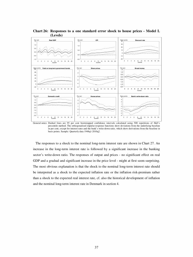
Chart 26: Responses to a one standard error shock to house prices - Model L

(Levels)

-1,0

-0,5

0,0

0,5

1,0

1,5

0 2 4 6 8 10 12 14 16 18 20Quarter

Per cent Real GDP

-0,5

0,0

0,5

1,0

1,5

0 2 4 6 8 10 12 14 16 18 20Quarter

Per cent CPI

-20

-10

0

10

20

30

40

0 2 4 6 8 10 12 14 16 18 20Quarter


-20

0

20

40

60

80

100

0 2 4 6 8 10 12 14 16 18 20Quarter


-6

-4

-2

0

2

4

0 2 4 6 8 10 12 14 16 18 20Quarter


-2,0

-1,5

-1,0

-0,5

0,0

0,5

1,0

1,5

0 2 4 6 8 10 12 14 16 18 20Quarter


-2,0

-1,5

-1,0

-0,5

0,0

0,5

1,0

1,5

0 2 4 6 8 10 12 14 16 18 20Quarter


-2

-1

0

1

2

3

4

0 2 4 6 8 10 12 14 16 18 20Quarter


-4

-3

-2

-1

0

1

2

3

4

0 2 4 6 8 10 12 14 16 18 20Quarter




The responses to a shock to the nominal long-term interest rate are shown in Chart 27. An

increase in the long-term interest rate is followed by a significant increase in the banking

sector’s write-down ratio. The responses of output and prices - no significant effect on real

GDP and a gradual and significant increase in the price level - might at first seem surprising.

The most obvious explanation is that the shock to the nominal long-term interest rate should

be interpreted as a shock to the expected inflation rate or the inflation risk-premium rather

than a shock to the expected real interest rate, cf. also the historical development of inflation

and the nominal long-term interest rate in Denmark in section 4.

37

Chart 27: Responses to a one standard error shock to the yield on long-term

government bonds - Model L (Levels)

-1,0

-0,5

0,0

0,5

1,0

1,5

0 2 4 6 8 10 12 14 16 18 20Quarter

Per cent Real GDP

-0,5

0,0

0,5

1,0

1,5

0 2 4 6 8 10 12 14 16 18 20Quarter

Per cent CPI

-20

-10

0

10

20

30

40

0 2 4 6 8 10 12 14 16 18 20Quarter


-20

0

20

40

60

80

100

0 2 4 6 8 10 12 14 16 18 20Quarter


-6

-4

-2

0

2

4

0 2 4 6 8 10 12 14 16 18 20Quarter


-2,0

-1,5

-1,0

-0,5

0,0

0,5

1,0

1,5

0 2 4 6 8 10 12 14 16 18 20Quarter


-2,0

-1,5

-1,0

-0,5

0,0

0,5

1,0

1,5

0 2 4 6 8 10 12 14 16 18 20Quarter


-2

-1

0

1

2

3

4

0 2 4 6 8 10 12 14 16 18 20Quarter


-4

-3

-2

-1

0

1

2

3

4

0 2 4 6 8 10 12 14 16 18 20Quarter




Responses to a shock to the bank’s write-down ratio

Finally, Chart 28 suggests that there are feedback effects from shocks to the banking sector to

the real economy. A shock to the bank’s write-down ratio - which might be interpreted as a

sudden reassessment of the credit quality of the bank’s loan portfolio or an increase in the

banking sectors’ risk aversion - has a significant and long-lasting negative effect on domestic

credit and real GDP. There thus seems to be a link between financial stability and

macroeconomic performance. The link might indicate the existence of a bank-lending

channel. According to such a line of thinking a shock to the bank’s capital is followed by a

period of reduced loan supply in order to maintain or re-establish a sufficient capital ratio, and

the reduced credit supply affects the other parts of the macroeconomic system. The negative

and persistent impact on real GDP after a shock to the banking sector’s write-down ratio is

consistent with the findings in the literature that economic recoveries after banking and

financial crises are slower than normal, cf. e.g. Bordo et al. (2001) and Reinhart & Reinhart

(2010).

38

Chart 28: Responses to a one standard error shock to bank’s write-down ratio -

Model L (Levels)

-1,5

-1,0

-0,5

0,0

0,5

0 2 4 6 8 10 12 14 16 18 20Quarter

Per cent Real GDP

-0,5

0,0

0,5

1,0

0 2 4 6 8 10 12 14 16 18 20Quarter

Per cent CPI

-40

-20

0

20

40

0 2 4 6 8 10 12 14 16 18 20Quarter


-60

-40

-20

0

20

0 2 4 6 8 10 12 14 16 18 20Quarter


-2

0

2

4

6

0 2 4 6 8 10 12 14 16 18 20Quarter


-2,0

-1,5

-1,0

-0,5

0,0

0,5

1,0

0 2 4 6 8 10 12 14 16 18 20Quarter


-2,5

-2,0

-1,5

-1,0

-0,5

0,0

0,5

1,0

0 2 4 6 8 10 12 14 16 18 20Quarter


-3

-2

-1

0

1

0 2 4 6 8 10 12 14 16 18 20Quarter


-2

0

2

4

6

8

0 2 4 6 8 10 12 14 16 18 20Quarter




7. Final remarks and scope for further research

Official quarterly national accounts for Denmark are only available for the period since 1977.

This paper has presented a first attempt to overcome this data shortage by constructing a set

of summary quarterly national-account data for Denmark covering the period since 1948. The

long-span data sets has made it possible to estimate VAR models of a higher dimension than

is usually found in the literature due to degrees-of-freedom problems. The estimated

responses to the shocks presented in the paper seem plausible and most of the responses are

clearly significant at 5 per cent levels. This illustrates the usefulness of long-span data sets

when the rich and complicated dynamic interactions between the financial sector and the real

economy are subject to study.

However, the quarterly national-account data presented in this paper should only be

considered as a first attempt to close some of the gaps in the existing stock of historical

statistics in Denmark. It could be useful if the data set on quarterly national accounts could be

disaggregated somewhat further, for instance with a breakdown of private consumption into

durables and non-durables and a drill-down of gross investment into sub-categories.

Furthermore, in general it would be preferable if the quarterly data could be based on a larger

39

set of indicators than the figures presented in section 3. Until now projects on historical

national accounts in Denmark have only focused on annual data.12 It would be interesting if

future projects on historical-national accounts statistics in Denmark would make an attempt to

cover quarterly data as well.

Also the supplementary quarterly data set in section 4 could benefit from further work. It

would be useful with quarterly data on employment and time series for public finances, at

least for the central government. It would also be interesting with a drill down of domestic

credit into commercial credit and credit to private individuals. Furthermore, as mentioned in

section 3 most of the quarterly data on the bank’s write-down ratio have been interpolated

from semi-annual or annual data. Even though the bank’s write-down ratio is rather persistent

in nature it could improve the quality of this data series if more quarterly information could

be uncovered.

The analysis of the stylised empirical evidence on the business cycle, the monetary

transmission mechanism and shocks to financial stability presented in this paper have only

been of an explorative nature. The data sets in section 3 and 4 could be subject to further and

more comprehensive studies. In Denmark there is no recognised business cycle dating

committee. The stylised facts on the business cycle in section 5 could therefore be elaborated

by an attempt to identify peaks and troughs in the Danish business cycle since 1948. Another

natural next step could be exploration of the robustness of the findings in section 6 within the

framework of cointegrated or structural VAR models.

8. References

Abildgren, K. (2009), Credit Dynamics in Denmark since World War II, Danish Journal of Economics, Vol. 147(1), pp. 89-119.

Agresti, A. M. & Mojon, B. (2003), Some stylised facts on the euro area business cycle, chapter 1 in: Angeloni, I., Kashyap, A. and Mojon, B. (eds.), Monetary Policy Transmission in the Euro Area, Cambridge: Cambridge University Press.

Anari, A., Kolari, J. & Mason, J. (2005), Bank Asset Liquidation and the Propagation of the U.S. Great Depression. Journal of Money, Credit and Banking, Vol. 37(4), pp. 753-773.

Baxter, M. & King, R. G. (1999), Measuring Business Cycles: Approximate Band-Pass Filters for Economic Time Series, Review of Economics and Statistics, Vol. 81(4), pp. 575-593.

Berner, O. & Thage, B. (1989), Kvartalsvise nationalregnskaber fra Danmarks Statistik – og nogle udenlandske erfaringer, Danish Journal of Economics, Vol. 127(1), pp. 95-109.

Berrospide, J. M. & Edge, R. M. (2010), The Effects of Bank Capital on Lending: What Do We Know, and What Does it Mean?, Federal Reserve Board Finance and Economics Discussion Series, No. 44, August.

Beier, N. C. & Storgaard, P. E. (2006), Identifying monetary policy in a small open economy under fixed exchange rates, Danmarks Nationalbank Working Paper, No. 38, June.

12 For an overview of the available historical national-accounts figures in Denmark, cf. pp. 164-179 in Mogensen (1987), Hyldtoft (1993, 1994), Christensen et al. (1995) and Nilsson (1991, 2004).

40

Blanchard, O. & Simon, J. (2001), The Long and large Decline in US Output Volatility, Brooking Papers on Economic Activity, No. 1, pp.135-164.

Bloem, A. M., Dippelsman, R. J. & Mæhle, N. Ø. (2001), Quarterly National Accounts Manual. Concepts, Data Sources, and Compilation, Washington DC: International Monetary Fund.

Boot, J. C. G., W. Feibes, and J. H. C. Lisman, 1967, Further Methods of Derivation of Quarterly Figures from Annual Data, Applied Statistics, Vol. 16(1), pp. 65–75.

Bordo, M., Eichengreen, B., Klingebiel, D. & Martinez-Peria, M. S. (2001), Is the Crisis Problem Growing More Severe?, Economic Policy, Vol. 16(32), pp. 53-82.

Busk-Nielsen, K., Hammer-Pedersen, K., Jensen, P. E. & Otholm, C. A. (1996), Dansk Bankvæsen i dag i morgen, Copenhagen: Forlaget FSR.

Carlsen, M. & Fæste, C. F. (2007), The Pass-Through from Danmarks Nationalbank's Interest Rates to the Banks' Retail Interest Rates, Danmarks Nationalbank Monetary Review, 2nd Quarter, pp. 23-37.

Christiano, L. J., Eichenbaum, M. and Evans, C. L. (1999), Monetary Policy Shocks: What Have We Learned and to What End?, in: Taylor, J. & Woodford, M. (eds.), Handbook of Macroeconomics, Amsterdam: North-Holland, 1999.

Christensen, A. M. (1989), Kvartalsvise nationalregnskaber i Nationalbanken, Danish Journal of Economics, Vol. 127(1), pp. 110-123.

Christensen, A. M. & Knudsen, D. (1992), MONA: a quarterly model of the Danish economy, Economic Modelling, Vol. 9(1), pp. 10-74.

Christensen, J. P., Hjerppe, R., Krantz, O. & Nilsson, C.-A. (1995), Nordic Historical National Accounts since the 1880s, Scandinavian Economic History Review, Vol. XLIII(1), pp. 30-52.

Ćorić, B. (2010), The Sources of the Great Moderation: A Survey, SSRN Working Paper, No. 1641201, July.

Danmarks Nationalbank (2003), MONA - a quarterly model of the Danish economy, Copenhagen: Danmarks Nationalbank.

Danmarks Nationalbank, Financial Stability, various issues. Danmarks Nationalbank, Monetary Review, various issues. Danmarks Nationalbank, Report and Accounts, various issues. Denton, F. T. (1971), Adjustment of Monthly or Quarterly Series to Annual Totals: An

Approach Based on Quadratic Minimization, Journal of the American Statistical Association, Vol. 66 (333), pp. 99-102.

DeJong, D. N. & Dave, C. (2007), Structurel Macroeconometrics, Princeton, NJ: Princeton University Press.

Dovern, J., Meier, C.-P. & Vilsmeier, J. (2010), How resilient is the German banking system to macroeconomic shocks?, Journal of Banking & Finance, Vol. 34 (8), pp. 1839–1848.

Enders, W. (2004), Applied Econometric Time Series, Second Edition, New Jersey: Wiley. Finanstilsynet, Markedsudviklingen for pengeinstitutter, various issues. Finanstilsynet, Pengeinstitutternes regnskaber, 1. halvår, various issues. Finanstilsynet (2008), Pengeinstitutternes regnskaber for 3. kvartal 2008, Copenhagen:

Finanstilsynet. Gencay, R., Selcuk, F. & Whitcher, B. (2002), An Introduction to Wavelets and Other

Filtering Methods in Finance and Economics, New York: Academic Press. Graversen, T. R., Haugaard, J., Petersen, J. D. & Südel, B. (2008), Quarterly National

Accounts Inventory. Sources and methods of the Quarterly National Accounts for Denmark, Copenhagen: Statistics Denmark.

Hamilton, J. D. (1994), Time Series Analysis, Princeton, NJ: Princeton University Press. Hansen, E. D., Kjærsgaard, K. & Rosted, J. (1988), Dansk økonomisk politik. Teorier og

erfaringer, Copenhagen: Erhvervsøkonomisk Forlag. Hansen, F. Ø. (2005), Samvariation i danske konjunkturcykler, Danmarks Nationalbank

Working Paper, No. 25, April.

41

Hansen, F. Ø. & Knudsen, D. (2004), Korrelationsmønstre i danske konjunkturcykler, Danish Journal of Economics, Vol. 143(3), pp. 257-273.

Hansen, J. & Paldam, M. (1973), SMEC. En kvartalsmodel af den danske økonomi, Copenhagen: Statens Trykningskontor.

Hoggarth, G., Sorensen, S. & Zicchino, L. (2005), Stress tests of UK banks using a VAR approach, Bank of England Working Paper, No. 282, November.

Hyldtoft, O. (1993), Danske historiske nationalindkomstberegninger, Danish Journal of Economics, Vol. 131, pp. 344-353.

Hyldtoft, O. (1994), Uløste problemer i danske historiske nationalregnskaber, Danish Journal of Economics, Vol. 132, pp. 92-102.

IMF, International Financial Statistics, various issues. Johansen, H. C. (1987), The Danish Economy In the Twentieth Century, London: Croom

Helm. Johansen, P. U. & Trier, M. (2010), Danmarks økonomi siden 1980 - en oversigt, 8th edition,

Copenhagen: Handelshøjskolens Forlag. King, R. G. & Watson, M. W. (1996), Money, Prices, Interest Rates and the Business Cycle,

Review of Economics and Statistics, Vol. 78(1), pp. 35-53. Krätzig, M. & Lütkepohl, H. (eds.) (2004), Applied Time Series Econometrics, New York:

Cambridge University Press. Kupiec, P. H. & Ramirez, C. D. (2008), Bank Failures and the Cost of Systemic Risk:

Evidence from 1900-1930, CFR Working Paper, No. 9, July. Kydland, F. E. & Prescott, E. C. (1990), Business Cycles: Real Facts and a Monetary Myth,

Federal Reserve Bank of Minneapolis Quarterly Review, Vol. 14, Spring, pp. 3-18. Marcucci, J. & Quagliariello, M. (2008), Is bank portfolio riskiness procyclical? Evidence

from Italy using a vector autoregression, Journal of International Finanacial Markets, Institutions and Money, Vol. 18, pp. 46–63.

Mikkelsen, R. (1993), Dansk pengehistorie 1960-1990, Copenhagen: Danmarks Nationalbank.

Mikkelsen, R. (1999), Marshall-hjælpen. Den Europæiske Betalingsunion, Copenhagen: Danmarks Nationalbank.

Mills, T. C. (2003), Modelling Trends and Cycles in Economic Time Series, New York: Palgrave.

Mogensen, G. V. (1987), Historie og økonomi, Copenhagen: Akademisk Forlag. Monnin, P. & Jokipii, T. (2010), The Impact of Banking Sector Stability on the Real

Economy, Swiss National Bank Working Paper, No. 5, April. Mordhorst, K. (1968), Dansk pengehistorie. Bilag, Copenhagen: Danmarks Nationalbank. Nilsson, C.-A. (1991), Er der behov for et HND?, Historisk Tidsskrift, Bind 91 Hæfte 1, pp.

218-226. Nilsson, C.-A. (2004), LAMEJSLA. Nye serier for landbrug og landbrugsindustri i de danske

historiske nationalregnskaber 1900-1947, Historisk Tidsskrift, Bind 104 Hæfte 1, pp. 229-241.

Pedersen, E. H. (1996), Real Effective Exchange Rates, Danmarks Nationalbank Monetary Review, May, pp. 33-45.

Pedersen, N. L. (1989), FINDAN. Finansiel sektor til ADAM, Rapport fra Modelgruppen, Danmarks Statistik Arbejdsnotat, No. 26.

Pedersen, P. J. (1996), Post-war growth of the Danish economy, chapter 17 in Crafts, N. & Toniolo, G. (eds.), Economic Growth in Europe Since 1945, Cambridge: Cambridge University Press.

Peersman, G. & Smets, F. (2003), The monetary transmission mechanism in the euro area: evidence from VAR analysis, chapter 2 in: Angeloni, I., Kashyap, A. and Mojon, B. (eds.) (2003), Monetary Policy Transmission in the Euro Area, Cambridge: Cambridge University Press.

Puddu, S. (2010), Real Sector and Banking System: Real and Feedback Effects. A Non-Linear VAR Approach, paper presented at the IEA Annual Conference, 23-25 April.

42

Reinhart, C. M. & Reinhart, V. R. (2010), After the Fall, paper presented at the Federal Reserve Bank of Kansas City Jackson Hole Symposium on “Macroeconomic Challenges: The Decade Ahead”, Wyoming, August 26-28.

Sims, C. A. (1972), Money, Income, and Causality, American Economic Review, Vol. 62(4), pp. 540-552.

Sims, C. A. (1980a), Macroeconomics and Reality, Econometrica, Vol. 48(1), pp. 1-48. Sims, C. A. (1980b), Comparison of Interwar and Postwar Business Cycles: Monetarism

Reconsidered, American Economic Review, Vol. 70(2), pp. 250-257. Sims, C. A., Stock, J. H. & Watson, M. W. (1990), Inference in Linear Time Series Models

with some Unit Roots, Econometrica, Vol. 58(1), pp. 113-144. Sløk, T. (1997), Er transmissionsmekanismen forskellig i Danmark og Tyskland?, Danish

Journal of Economics, Vol. 135(2), pp. 135-143. Statistics Denmark (1966), Nationalregnskabsstatistik 1947-1960, Statistiske Undersøgelser,

No. 7, Copenhagen: Statistics Denmark. Statistics Denmark (1969), Kreditmarkedsstatistik, Statistiske Undersøgelser, No. 24,

Copenhagen: Statistics Denmark. Statistics Denmark (1995), 50-year review, Copenhagen: Statistics Denmark. Statistics Denmark (1996), Arbejdsløshedsserier 1910-1995, Statistiske Efterretninger.

Arbejdsmarked, No. 28, 24 October. Statistics Denmark, Statistiske Efterretninger, various issues. Statistics Denmark, Konjunkturoversigt, various issues. Statistics Denmark, Statistisk Månedsoversigt, various issues. Statistics Denmark, Statistical ten-year review, various issues. Statistics Denmark, Statistical Yearbook, various issues. Statistics Denmark, StatBank Denmark, Statistics Denmark’s website (www.dst.dk). Stock, J. H. & Watson, M. W. (1999), Business Cycle Fluctuations in US Macroeconomic

Time Series, in: Taylor, J. B. and Woodford, M., (eds.) Handbook of Macroeconomics, Volume 1A, Amsterdam: Elsevier.

Stock, J. H. & Watson, M. W. (2001), Vector Autoregressions, Journal of Economic Perspectives, Vol. 15(4), pp. 101–115.

Stock, J. H. & Watson, M. W. (2003), Has the Business Cycle Changed? Evidence and Explanations, paper presented at the Federal Reserve Bank of Kansas City Jackson Hole Symposium on “Monetary Policy and Uncertainty: Adapting to a Changing Economy”, Wyoming, August 28-30.

Sørensen, R. S. (1994a), Kvartalsvise nationalregnskaber 1977-1986 (dokumentation og tabeller), Danmarks Statistik Nationalregnskabsnotat, Arbejdsnotat, nr. 37, September.

Sørensen, R. S. (1994a), Sæsonkorrigering af de kvartalsvise nationalregnskaber, Danmarks Statistik Nationalregnskabsnotat, Arbejdsnotat, nr. 35, April.

Sørensen, R. S. (1994c), Analyse af 80ernes økonomiske udvikling baseret på kvartalsvise nationalregnskaber, Danmarks Statistik Statistiske Undersøgelser, No. 45, September.

Thygesen, N. (1971), The Sources and the Impact of Monetary Changes. An Empirical Study of Danish Experiences 1951-68, Copenhagen: GADs Forlag.

U.S. Census Bureau (2009), X-12-ARIMA Reference Manual. Version 0.3, December. Walsh, C. E. (2010), Monetary Theory and Policy, Third Edition, Cambridge Mass.: MIT

Press. Økonomiministeriet (1994), Den danske pengeinstitutsektor, Copenhagen: Schultz. Økonomiministeriet (1997), Økonomiministeriet i 50 år 1947-1997, Copenhagen: Schultz. Ølgaard, C. (1992), The Effective Krone Rate and Competitiveness, Danmarks Nationalbank

Monetary Review, February, pp. 8-15. Österholm, P. (2010), The effect on the Swedish real economy of the financial crisis, Applied

Financial Exonomics, Vol. 20(4), pp. 265-274.

43

Annex A: Data sources

National accounts statistics, annual data 1948-1971

Sources:

Various issues of Statistics Denmark, Statistiske Efterretninger; and Statistics Denmark,

Statistical ten-year review. Other sources: Statistics Denmark (1966).

Comments:

(1) Figures in constant prices are based on 1955-prices.

National accounts statistics (non-seasonally adjusted), quarterly data 1971q1-1977q4

Sources:

The MONA database (cf. Danmarks Nationalbank, 2003) and Statistics Denmark, StatBank

Denmark.

(1) The non-seasonally adjusted data been compiled on the basis of seasonally adjusted data

and seasonal factors from 1977. (2) Figures in constant prices are based on 2000-prices (chain

figures).

National accounts statistics (non-seasonally adjusted), quarterly data 1977q1-2010q2

Sources:

Statistics Denmark, StatBank Denmark.

Comments:

(1) Adjusted for break in series in 1988 and 1990. (2) Figures in constant prices are based on

1995-prices (1988-1990) and 2000-prices (1991-2010).

Value index for retail sales, quarterly data 1948q1-1971q4

Sources:

Various issues of Statistics Denmark, Statistical Yearbook.

Comments:

(1) Adjusted for break in series in 1955, 1961 and 1968. Consumer price index, Denmark, quarterly data 1948q1-2010q2

Sources:


Statistical Yearbook.

Comments:

(1) Adjusted for break in series in 1956, 1965, 1976, 1981 and 2000.

44

Number of new registrations of passenger cars etc., quarterly data 1948q1-1971q4

Sources:


Konjunkturoversigt;

Comments:

(1) Adjusted for break in series in 1949 and 1955. Number of dwellings started, quarterly data 1948q1-1971q4

Sources:



Comments:

(1) 1969-1971: Quarterly data for the number of dwellings started in all of Denmark. (2) For

the period 1949-1968 are the quarterly data estimated on the basis of semiannual data for the

number of dwellings started in all of Denmark and quarterly data for the number of dwellings

started in towns etc. with more than 1000 inhabitants. During the period 1949-1968 the

number of dwellings started in towns etc. with more than 1000 inhabitants covered 75-87 per

cent of the number of dwellings started in all of Denmark. (3) For 1948 are the quarterly data

estimated on the basis of the development in quarterly data for the number of dwellings

started in town etc. with more than 1000 inhabitants. (4) Adjusted for break in series 1949 and

1969.

Index of building costs, quarterly data 1948q1-1971q4 Sources:


Comments:

(1) 1968-1971: Index of building costs for a single-family house. 1949-1967: Index of

building costs for a residential building. 1948: index of building costs of a 3-storeyed

building.

(2) Adjusted for break in series in 1949, 1955 and 1968.

45

Gross floor space (m2) of new buildings started excluding dwellings started, quarterly data

1948q1-1971q4

Sources:



Comments:

(1) Quarterly figures for gross floor space of new dwellings started is calculated on the basis

of gross floor space of new dwellings started in 1948 and the development in the number of

dwellings started on a quarterly basis in the period 1948-1971. (2) Adjusted for break in series

in 1949, 1963 and 1968.

Number of new registrations of commercial vehicles, quarterly data 1948q1-1971q4

Sources:

Various issues of Statistics Denmark, Statistiske Efterretninger; Statistics Denmark,

Konjunkturoversigt; and Statistics Denmark, Statistical Yearbook.

Wholesale price index, quarterly data 1948q1-1971q4

Sources:

Various issues of Statistics Denmark, Statistical Yearbook; and IMF, International Financial

Statistics.

Comments:

(1) Adjusted for break in series in 1955, 1956 and 1968.

Value of exports and imports of goods, quarterly data 1948q1-1971q4

Sources:


Comments:

(1) 1948-1956: Special trade. 1957-1971: General trade. (2) Adjusted for break in series in

1957.

Index of unit values in exports and imports of goods, quarterly data 1948q1-1971q4

Sources:


Comments:

(1) Excluding ships and aeroplanes. (2) Adjusted for break in series in 1949, 1956, 1966 and

1971.

46

Value of exports and imports of services, quarterly data 1948q1-1971q4 Sources:

Various issues of Danmarks Nationalbank, Annual Report and Accounts; and Statistics

Denmark, Statistical Yearbook. Other sources: Thygesen (1971).

Comments:

(1) Quarterly data for the value of exports and imports of services are only available from

1960. Prior to 1960 the figures are interpolated based on the development in the value of

exports and imports of goods.

Unemployment rate, quarterly data 1948q1-2010q2 Sources:

Various issues of: Statistics Denmark, Statistical ten-year review. Other sources: Statistics

Denmark (1996); and Statistics Denmark, StatBank Denmark.

Comments:

(1) Unemployed persons in per cent of the total labour force. (2) For the period 1966-1972

calculated on the basis of annual data for unemployed persons in per cent of the total labour

force and quarterly data for unemployed persons in per cent of wage earners in the labour

force (3) For the period 1948-1965 calculated on the basis of annual data for unemployed

persons in per cent of the total labour force 1949-1965 and quarterly data for unemployed

members of unemployment insurance funds in per cent of the total number of members of

unemployment insurance funds 1948-1965. (4) Adjusted for break in series in 1949, 1957,

1966, 1973, 1980 and 2000.

Index of average hourly earnings in manufacturing industries, quarterly data 1948q1-

2010q2 Sources:

Various issues of: Statistics Denmark, Statistical Yearbook. Other sources: Statistics

Denmark, StatBank Denmark.

Comments:

(1) Adjusted for break in series in 1970, 1973, 1996 and 2007.

Official discount rate of Danmarks Nationalbank, quarterly data 1948q1-2010q2

Sources:

Various issues of: Danmarks Nationalbank, Report and Accounts. Other sources: Mordhorst

(1968); and Danmarks Nationalbank’s website (www.nationalbanken.dk).

Comments:

(1) Quarterly averages of daily observations.

47

Yield on long-term Danish government bonds, quarterly data 1948q1-2010q2

Sources:

Various issues of: Danmarks Nationalbank, Monetary Review; and Danmarks Nationalbank,

Report and Accounts. Other sources: Danmarks Nationalbank’s website

(www.nationalbanken.dk); Statistics Denmark (1969) and internal material from Danmarks

Nationalbank.

Comments:

(1) 1983q3-2010q2: Yield to maturity on 10-year central government bonds. 1948q1-1983q2:

Yield to maturity on long central government bonds. (2) 1960-2010: Quarterly averages of

daily observations. 1948-1959: The quarterly figures refer to 15 March, 15 June, 15

September and 15 December.

Private banks’ average lending rate, quarterly data 1948q1-2010q2 Sources:

Various issues of: Danmarks Nationalbank, Report and Accounts; and Statistics Denmark,

Statistical Yearbook. Other sources: Carlsen & Fæste (2007); Mikkelsen (1993); Pedersen

(1989); Thygesen (1971); and Danmarks Nationalbank’s website (www.nationalbanken.dk).

Comments:

(1) Quarterly data for the weighted average lending interest rates of savings banks and

commercial banks are only available for the period 1973-2010. For the period 1969-1972 the

quarterly data are based on annual data on the weighted average lending interest rates of

savings banks and commercial banks and quarterly data for the average lending rate charged

by the main commercial banks. For the period 1951-1968 are the quarterly data based on

annual data on the weighted average lending interest rates of savings banks and commercial

banks and quarterly data for the rate charged by commercial banks on cash credits. For the

period 1948-1950 the quarterly data are based on annual data on the weighted average lending

interest rates of savings banks and commercial banks and quarterly data for the average

lending rate charged by the main commercial banks. (2) Adjusted for break in series in 1948,

1951, 1969, 1973, 1976 and 1983.

48

Private banks’ average deposit rate, quarterly data 1948q1-2010q2

Sources:

Various issues of: Danmarks Nationalbank, Report and Accounts; and Statistics Denmark,

Statistical Yearbook. Other sources: Carlsen & Fæste (2007); Mikkelsen (1993); Pedersen

(1989); Thygesen (1971); and Danmarks Nationalbank’s website (www.nationalbanken.dk).

Comments:

(1) Quarterly data for the weighted average deposit interest rates of savings banks and

commercial banks are only available for the period 1973-2010. For the period 1969-1972 the

quarterly data are based on annual data on the marginal between the weighted average lending

and deposits rates of savings banks and commercial banks and quarterly data for the private

banks’ average lending rate. For the period 1951-1968 based on quarterly data on the

marginal between the weighted average lending and deposits rates of commercial banks and

quarterly data for the private banks’ average lending rate. For the period 1948-1950 the

quarterly data are based on annual data on the weighted average deposit interest rates of

savings banks and commercial banks (2) Adjusted for break in series in 1951, 1969, 1976 and

1983.

Nominal effective krone-rate index, quarterly data 1948q1-2010q2

Sources:

Various issues of: Danmarks Nationalbank, Report and Accounts; and Danmarks

Nationalbank, Monetary Review. Other sources: Danmarks Nationalbank’s website

(www.nationalbanken.dk), Pedersen, E. H. (1996), Statistics Denmark (1995) and Ølgaard

(1992).

Comments:

(1) Trade-weighted average of the development in the bilateral nominal krone-rate vis-à-vis

the currencies of a range of Denmark’s main trading partners. An increase in the index

describes an overall nominal appreciation of the Danish krone vis-à-vis the currencies of

Denmark’s main trading partners. (2) Quarterly averages. (3) 1970-2010: Based on the

official nominal effective krone-rate index published by the Nationalbank. The index has been

compiled by weighting (geometrically) the development in indices for the bilateral value of

one krone vis-à-vis the currency range of different countries. The weights used in the index

are based on so-called double-weighted export weights and bilateral import weights. For the

period from 8 April 2010 to June 2010 the official nominal effective krone-rate index is based

on weights calculated from 2009 trade statistics (covering trade with 27 countries). For the

period from 1 October 2004 to 7 April 2010 the official nominal effective krone-rate index is

based on weights calculated from 2002 trade statistics (covering trade with 27 countries). The

49

weights from the period 30 May 1997 to 30 September 2004 are based on 1995 trade statistics

(25 countries). For the period from 1 January 1992 to 29 May 1997 the weights are based on

1989 trade statistics (21 countries). For 1970-1991 the weights are based on 1983 trade

statistics (17 countries). (4) No official quarterly nominal effective krone-rate index has been

published by the Nationalbank for the period prior to 1970. For the period 1948-1969 the

index has been compiled by weighting (geometrically) the development in indices for the

bilateral value of one krone vis-à-vis the currencies of 9 different countries (Germany, U.K.,

Sweden, Norway, U.S.A., France, The Netherlands, Finland and Switzerland) using the 1983-

weights mentioned above. (5) Adjusted for break in series in 1970.

Consumer price index, abroad, quarterly data 1948q1-2010q2 Sources:

Various issues of Statistics Denmark, Statistical Yearbook. Other sources: Danmarks

Nationalbank’s website (www.nationalbanken.dk), Pedersen, E. H. (1996) and Ølgaard

(1992).

Comments:

(1) Trade-weighted average of the consumer price development in Denmark’s main trading

partners. The weights and weighting methodology are identical to those used for the

calculation of the nominal effective krone-rate index, cf. the description above. (2) Quarterly

averages. (3) Adjusted for break in series in 1970.

Consumer price index, West Germany, quarterly data 1948q1-1970q4 Sources:


Comments:

(1) Adjusted for break in series in 1950, 1951, 1952, 1954, 1961, 1962, 1965 and 1968.

Consumer price index, U.K., quarterly data 1948q1-1970q4

Sources:


Comments:


Consumer price index, Sweden, quarterly data 1948q1-1970q4

Sources:


Comments:


50

Consumer price index, Norway, quarterly data 1948q1-1970q4

Sources:


Comments:


Consumer price index, U.S.A., quarterly data 1948q1-1970q4

Sources:


Comments:


Consumer price index, France, quarterly data 1948q1-1970q4

Sources:


Comments:

(1) Adjusted for break in series in 1950, 1955, 1957, 1960, 1962, 1964, 1965 and 1968.

Consumer price index, The Netherlands, quarterly data 1948q1-1970q4

Sources:


Comments:

(1) Adjusted for break in series in 1951, 1953, 1954, 1961, 1962, 1965 and 1968.

Consumer price index, Finland, quarterly data 1948q1-1970q4

Sources:


Comments:


Consumer price index, Switzerland, quarterly data 1948q1-1970q4

Sources:


Comments:


51

Real effective krone-rate index with consumer prices as deflator 1948q1-2010q2

Comments:

(1) The weights and weighting methodology are identical to those used for the calculation of

the nominal effective krone-rate index, cf. the description above.

Price index for sale of one-family houses, quarterly data 1948q1-2010q2

Sources:

Various issues of Statistics Denmark, Statistiske Efterretninger. Other sources: Thygesen

(1971); and Statistics Denmark, StatBank Denmark.

Comments:

(1) 1948-1950: Covers the price development on sales of smallholdings. 1951-1967: Covers

the price development for sale of one-family houses in provincial towns. 1968-2010: Covers

the cash-price development for one-family houses in ordinary free trade in all of Denmark. (2)

Adjusted for break in series 1950 and 1968.

Share price index, quarterly data 1948q1-2010q2

Sources:

Various issues of: Statistics Denmark, Statistics Månedsoversigt and Statistics Denmark,

Statistical Yearbook. Other sources: Danmarks Nationalbank’s website

(www.nationalbanken.dk).

Comments:

(1) End of quarter. (2) 1948-1993: Covers all shares at the Copenhagen Stock Exchange.

1994-2010: OMXC20 (KFX). (3) Adjusted for break in series in 1957, 1959, 1964, 1972,

1982 and 1994.

Broad money stock (M2), quarterly data 1948q1-2010q2 Various issues of: Danmarks Nationalbank, Report and Accounts. Other sources: Thygesen

(1971); and Danmarks Nationalbank’s website (www.nationalbanken.dk).

Comments:

(1) End of quarter. (2) For the period prior to 1993 calculated on the basis of year-to-year

growth rates where adjustments have been made for break in series.

52

Credit to the domestic non-bank sector extended by resident commercial banks and savings

banks, quarterly data 1948q1-2010q2

Various issues of: Danmarks Nationalbank, Report and Accounts. Other sources: Danmarks

Nationalbank’s website (www.nationalbanken.dk).

Comments:

(1) End of quarter. (2) Covers commercial banks and savings banks. (3) For the period prior

to 1981 calculated on the basis of year-to-year growth rates where adjustments have been

made for break in series.

Credit to the domestic non-bank sector extended by resident mortgage banks, quarterly data

1948q1-2010q2 Various issues of: Danmarks Nationalbank, Report and Accounts. Other sources: Danmarks

Nationalbank’s website (www.nationalbanken.dk).

Comments:

(1) End of quarter. (2) For the period 1961-1981 calculated on the basis of accumulated flow-

of-funds figures regarding the net supply of Danish mortgage-credit bonds at market values

(1964-1981) or nominal values (1961-1963). (3) For the period 1948-1956 are the quarterly

figures interpolated from annual data. (4) Adjusted for break in series in 1957, 1961 and

1981.

Bank’s write-downs ratio, quarterly data 1948q1-2010q2

Sources:

Various issues of: Danmarks Nationalbank, Financial Stability; Finanstilsynet,

Markedsudviklingen for pengeinstitutter; Finanstilsynet, Pengeinstitutternes regnskaber, 1.

halvår; and Statistics Denmark, Statistical Yearbook. Other sources: Busk-Nielsen et al.

(1996); Finanstilsynet (2008) and Økonomiministeriet (1994).

Comments:

(1) Quarterly write-downs on loans and guaranties in per cent of end-quarter outstanding

loans and guaranties. The write-down ratios are not annualised and are compiled net of

receipts on relinquished debts. (2) Covers write-downs in commercial banks and savings

banks. (3) For the period 1991-2010 based on quarterly or semi-annual data. For the period

1948-1990 are the quarterly data interpolated from annual data using the least-squares-based

method described in Boot et al. (1967).

53

Annex B: Summary quarterly national accounts for Denmark 1948-2010

Table B.1: Quarterly national accounts data, current prices, non-seasonally adjusted, 1948q1-2010q2 Private

consumption Government consumption

Gross investments Exports of goods and services

Imports of goods and services

Gross Domestic Product

Quarter

million kroner 1948q1 2591 500 959 992 819 4223 1948q2 2765 500 816 877 1021 3937 1948q3 2703 515 1181 990 1216 4173 1948q4 3121 543 1350 1064 1241 4839 1949q1 2713 520 1059 1071 1302 4060 1949q2 2935 524 1002 1182 1355 4288 1949q3 2896 542 1143 1232 1252 4560 1949q4 3392 570 1229 1446 1348 5289 1950q1 3042 542 1195 1353 1750 4381 1950q2 3289 550 1386 1441 1627 5040 1950q3 3463 582 1481 1719 1969 5276 1950q4 3867 636 1548 1812 1916 5948 1951q1 3447 633 1367 1891 1959 5378 1951q2 3632 660 1362 2051 2352 5352 1951q3 3517 702 1554 2043 2251 5565 1951q4 3991 758 1302 2276 2059 6269 1952q1 3552 734 1336 2190 2219 5593 1952q2 3701 748 1383 1915 1992 5755 1952q3 3701 784 1542 2252 2074 6205 1952q4 4140 836 1610 2094 2096 6583 1953q1 3664 804 1475 2180 2168 5954 1953q2 3879 817 1576 2056 1974 6354 1953q3 3874 855 1848 2158 2313 6423 1953q4 4267 915 1853 2299 2246 7087 1954q1 3813 885 1716 2174 2155 6433 1954q2 4224 900 1658 2325 2524 6582 1954q3 4270 936 1953 2393 2657 6895 1954q4 4533 990 1677 2416 2614 7002 1955q1 4230 941 1440 2477 2486 6601 1955q2 4335 947 1331 2505 2453 6664 1955q3 4340 982 1949 2598 2684 7184 1955q4 4803 1042 1864 2743 2634 7818 1956q1 4412 1000 1794 2616 2459 7363 1956q2 4649 1012 1578 2774 2887 7126 1956q3 4672 1052 2166 2854 3001 7742 1956q4 5086 1114 1934 2924 3086 7972 1957q1 4556 1064 1958 2882 3206 7253 1957q2 4875 1073 2218 2996 2850 8311 1957q3 4727 1113 2296 3164 3024 8276 1957q4 5169 1177 1890 3169 2987 8419 1958q1 4705 1125 1704 3039 2794 7778 1958q2 4979 1138 1782 3107 2686 8319 1958q3 5026 1187 2227 3149 3309 8281 1958q4 5556 1267 2155 3293 3096 9175 1959q1 5110 1224 2019 3121 2981 8493 1959q2 5393 1242 2402 3165 3348 8854 1959q3 5374 1288 2821 3664 3599 9548 1959q4 5959 1357 2860 3688 3821 10043 1960q1 5389 1284 2804 3488 3888 9077 1960q2 5848 1301 2958 3652 3679 10080 1960q3 5818 1373 3115 3726 3785 10246 1960q4 6402 1496 2789 3794 4011 10470 1961q1 5937 1487 3099 3584 3898 10209 1961q2 6309 1559 3342 3614 3755 11068 1961q3 6617 1677 3140 3912 4135 11210 1961q4 7221 1838 3108 3990 4311 11846 1962q1 6713 1817 3393 3861 4267 11517 1962q2 7369 1876 3638 3938 4318 12504 1962q3 7518 1971 4264 4089 4954 12889 1962q4 7711 2094 3501 4329 4676 12959 1963q1 7036 1992 3180 4155 4140 12223 1963q2 7680 2016 2907 4625 4587 12640 1963q3 7950 2113 3848 4715 4825 13801 1963q4 8403 2277 4013 4813 4856 14650 1964q1 7887 2228 4071 4728 5035 13879 1964q2 8469 2306 4404 4873 5666 14386 1964q3 8835 2456 4679 5269 5566 15674 1964q4 9427 2673 4941 5698 5928 16812 1965q1 8902 2628 5631 5311 5862 16609 1965q2 9216 2721 4895 5589 6121 16300

54

Table B.1 (continued): Quarterly national accounts data, current prices, non-seasonally adjusted, 1948q1-2010q2 Private





Quarter


55






Quarter


56






Quarter

million kroner 2000q3 151460 81505 61638 156934 132407 319130 2000q4 161550 84029 70692 170498 143813 342956 2001q1 154266 81838 62566 156461 133926 321205 2001q2 157922 85322 69786 157499 137455 333074 2001q3 155069 86600 66784 155949 132951 331451 2001q4 164430 89504 72843 160976 137873 349880 2002q1 158846 86571 68217 154176 139251 328559 2002q2 161401 90280 74583 162437 143129 345572 2002q3 160037 90816 67669 161800 139595 340727 2002q4 171972 92545 69674 169903 146215 357879 2003q1 163052 89145 68692 155344 137393 338840 2003q2 163566 93009 68941 154794 132870 347440 2003q3 162756 93103 63892 159908 133956 345703 2003q4 177568 95979 73439 165068 143347 368707 2004q1 169662 94272 69464 155406 137600 351204 2004q2 173329 97602 74170 166962 146644 365419 2004q3 173137 97058 76318 168217 151313 363417 2004q4 191086 100097 78553 174419 158014 386141 2005q1 177569 97379 72325 167351 152265 362359 2005q2 186752 100467 83449 189616 168583 391701 2005q3 182884 100432 79039 197004 173474 385885 2005q4 197934 104230 86994 203034 186880 405312 2006q1 190787 102448 81639 200479 188238 387115 2006q2 198715 105224 97478 210660 197323 414754 2006q3 190486 105542 94662 216857 198764 408783 2006q4 206594 109390 96836 221606 213420 421006 2007q1 198159 106703 96871 210880 206996 405617 2007q2 204183 108854 98217 216662 206872 421044 2007q3 200195 109157 95723 225113 209391 420797 2007q4 219128 114416 98609 233727 221866 444014 2008q1 208171 110535 93608 227651 221028 418937 2008q2 216255 114684 98933 246369 233641 442600 2008q3 207412 116711 93774 248874 231023 435748 2008q4 213673 121882 95088 233017 223497 440163 2009q1 199433 119270 78141 194073 185215 405702 2009q2 203853 123269 70651 191633 178098 411308 2009q3 200411 124583 69265 198159 177912 414506 2009q4 213885 129260 71644 201357 185293 430853 2010q1 211354 126187 63838 197361 179579 419161 2010q2 213817 129691 75635 222240 198772 442611

57

Table B.2: Quarterly national accounts data, constant prices, non-seasonally adjusted, 1948q1-2010q2 Private





Quarter

million 2000-kroner 1948q1 39307 12935 13565 6624 5413 67018 1948q2 40954 13028 11179 5836 7269 63727 1948q3 40395 13417 16580 6941 8653 68680 1948q4 44239 13770 17694 7492 8455 74741 1949q1 39773 13090 13415 7184 8557 64906 1949q2 41884 13183 13329 7939 9790 66546 1949q3 41917 13510 15758 8410 9360 70236 1949q4 46365 13731 17417 9689 8992 78210 1950q1 42157 12863 14684 8492 10552 67645 1950q2 43727 12944 17589 9291 10670 72882 1950q3 45490 13439 19120 11705 12743 77011 1950q4 47699 14026 19143 11981 12076 80773 1951q1 43025 13670 14855 10852 10551 71852 1951q2 43795 14084 14194 11591 11491 72172 1951q3 42783 14738 18497 12023 11226 76815 1951q4 46141 15273 14730 12198 10159 78182 1952q1 42513 14570 13167 11223 10112 71360 1952q2 43749 14832 13018 10303 10111 71792 1952q3 44004 15475 17033 13318 11582 78248 1952q4 47206 16124 18012 12028 11533 81837 1953q1 43135 15593 15166 12050 11366 74578 1953q2 44931 15989 16374 11657 11275 77676 1953q3 45401 16699 20787 13504 13735 82656 1953q4 48327 17317 19869 14089 12843 86758 1954q1 44886 16573 18092 12481 11615 80418 1954q2 48189 16823 15442 13400 14749 79106 1954q3 49025 17401 21220 14865 15794 86717 1954q4 50506 17873 18832 14489 15139 86561 1955q1 47701 16946 14682 13840 13158 80011 1955q2 48001 17062 12051 14103 14297 76920 1955q3 48025 17523 21573 15818 15809 87130 1955q4 50616 17891 20035 15389 14952 88978 1956q1 47517 16879 18555 13846 12831 83965 1956q2 49046 17000 13974 14822 15858 78983 1956q3 49422 17559 21583 16030 16631 87962 1956q4 51830 18124 18493 16162 16913 87696 1957q1 47620 17376 17225 15061 15859 81423 1957q2 50259 17625 20114 15930 15293 88636 1957q3 48920 18172 21762 17665 16861 89659 1957q4 51964 18561 18134 18240 16349 90551 1958q1 48848 17456 15201 16663 14994 83173 1958q2 50965 17586 15218 17749 15577 85941 1958q3 51918 18228 22182 19038 19523 91842 1958q4 55216 18941 20345 18959 17862 95599 1959q1 51803 18334 17586 16660 16810 87573 1959q2 53681 18788 19401 17908 19776 90002 1959q3 53872 19584 26291 20924 21654 99017 1959q4 57103 20239 26355 21226 22167 102757 1960q1 52958 19278 24427 19027 21328 94361 1960q2 56135 19535 23422 20643 20913 98824 1960q3 56276 20231 27711 21733 22420 103531 1960q4 59751 20867 24351 21974 23114 103828 1961q1 56695 19923 26051 19826 21566 100929 1961q2 58883 20362 28088 19767 21465 105635 1961q3 61177 21392 25167 23036 24154 106618 1961q4 64380 22505 24128 24007 24732 110288 1962q1 60857 22024 25222 20633 23589 105147 1962q2 64680 22686 25487 21257 24559 109551 1962q3 65902 23640 33929 23629 28283 118818 1962q4 64638 24299 27990 24887 27229 114585 1963q1 60060 22902 24619 21670 22650 106600 1963q2 63509 23138 18968 24556 25887 104283 1963q3 65995 24066 29792 26106 27534 118426 1963q4 67821 25110 29650 26134 27000 121715 1964q1 64730 24415 30215 23575 26749 116185 1964q2 67664 25076 29673 24828 31369 115872 1964q3 70199 26144 33297 28318 31164 126794 1964q4 72451 26971 33964 31093 32255 132225 1965q1 69329 25596 38221 26435 30738 128842 1965q2 70128 25912 32060 27892 32866 123125

58

Table B.2 (continued): Quarterly national accounts data, constant prices, non-seasonally adjusted, 1948q1-2010q2 Private





Quarter


59






Quarter


60






Quarter

million 2000-kroner 2000q3 151013 81086 62978 156204 131490 319791 2000q4 160079 83273 69651 164486 139404 338085 2001q1 152339 80885 62293 154249 132250 317516 2001q2 154080 82300 68570 153119 133555 324514 2001q3 151104 83386 64870 153192 130425 322127 2001q4 159662 85662 70862 160680 137938 338928 2002q1 153806 82555 67625 155577 141109 318454 2002q2 155199 84840 72336 162740 145047 330068 2002q3 153928 85292 64998 162399 142292 324325 2002q4 164169 87067 66006 169219 148602 337859 2003q1 154713 83875 68007 157155 141426 322324 2003q2 155286 85563 66431 157779 137434 327625 2003q3 155217 85461 58464 160764 138239 321667 2003q4 168351 87980 70733 166402 148591 344875 2004q1 160219 85856 65651 159028 144929 325825 2004q2 162510 87618 71396 168182 152245 337461 2004q3 163254 86715 72724 165426 154822 333297 2004q4 178966 89078 73142 169740 159657 351269 2005q1 165590 86651 66770 164689 157260 326440 2005q2 173374 88391 77415 184974 174041 350113 2005q3 169632 88132 71475 186820 173810 342249 2005q4 181199 91470 81539 192399 186415 360192 2006q1 175562 89338 75049 185929 185496 340382 2006q2 181061 90663 89319 195795 194101 362737 2006q3 172581 90751 85336 196133 191494 353307 2006q4 187690 93707 87216 204148 203769 368992 2007q1 178815 91124 85292 194295 197845 351681 2007q2 182474 91609 87440 197308 195155 363676 2007q3 179192 91186 83135 203237 196070 360680 2007q4 194964 95326 87909 204919 204164 378954 2008q1 182815 91430 82250 197552 200869 353178 2008q2 187859 93002 85988 210071 208661 368259 2008q3 178754 93357 81254 208273 203278 358360 2008q4 184420 97171 84688 203044 204445 364878 2009q1 172274 94808 69460 182460 180684 338318 2009q2 174892 96047 63740 181900 173585 342994 2009q3 171288 96784 61735 185174 174834 340147 2009q4 183732 100165 65051 186145 180249 354844 2010q1 178987 97143 59199 178319 173343 340305 2010q2 179612 98891 70557 191001 185337 354724

61

Annex C: Other key quarterly macroeconomic indicators for Denmark 1948-

2010

Table C.1: Quarterly key macroeconomic indicators, non-seasonally adjusted, 1948q1-2010q2 Unemployment

rate Index of average

hourly earnings in manufacturing

Official discount rate of Danmarks Nationalbank

Yield on long-term Danish government

bonds

Private banks’ average lending

rate

Private banks’ average deposit rate

Quarter

Per cent of the labour force

2005q1=100 Per cent per annum Per cent per annum Per cent per annum Per cent per annum

1948q1 3.8 1.42 3.50 3.90 3.89 1.59 1948q2 2.1 1.53 3.50 4.00 3.89 1.59 1948q3 1.8 1.51 3.50 4.10 3.89 1.59 1948q4 2.8 1.56 3.50 4.40 3.89 1.59 1949q1 1.9 1.52 3.50 4.50 4.37 1.80 1949q2 4.6 1.60 3.50 4.50 4.37 1.80 1949q3 3.0 1.57 3.50 4.30 4.37 1.80 1949q4 2.5 1.61 3.50 4.40 4.37 1.80 1950q1 3.3 1.55 3.50 4.30 4.22 1.56 1950q2 3.2 1.68 3.50 4.40 4.22 1.56 1950q3 2.3 1.65 4.47 4.60 5.08 2.43 1950q4 2.0 1.71 4.83 4.80 5.41 2.75 1951q1 2.8 1.69 5.00 4.90 5.46 2.40 1951q2 2.7 1.83 5.00 5.10 5.48 2.43 1951q3 3.3 1.82 5.00 5.20 5.51 2.47 1951q4 3.2 1.92 5.00 5.30 5.54 2.50 1952q1 1.6 1.85 5.00 5.30 5.60 2.55 1952q2 5.3 1.98 5.00 5.30 5.63 2.57 1952q3 5.6 1.96 5.00 5.30 5.66 2.58 1952q4 2.7 2.03 5.00 5.20 5.68 2.59 1953q1 3.1 1.95 5.00 5.20 5.74 2.63 1953q2 4.0 2.04 5.00 5.10 5.75 2.64 1953q3 2.9 2.00 4.96 5.10 5.71 2.66 1953q4 2.0 2.05 4.50 5.00 5.38 2.66 1954q1 5.0 1.97 4.50 5.00 5.67 2.89 1954q2 2.3 2.20 4.59 5.10 5.78 2.88 1954q3 1.8 2.07 5.50 5.40 6.37 3.20 1954q4 1.2 2.14 5.50 5.60 6.37 3.22 1955q1 3.9 2.07 5.50 5.40 6.31 3.17 1955q2 2.7 2.26 5.50 5.60 6.32 3.18 1955q3 2.4 2.15 5.50 5.60 6.33 3.19 1955q4 3.3 2.26 5.50 5.60 6.33 3.20 1956q1 5.4 2.19 5.50 5.60 6.37 3.23 1956q2 4.2 2.44 5.50 5.60 6.39 3.24 1956q3 2.9 2.32 5.50 5.70 6.40 3.25 1956q4 1.9 2.47 5.50 5.80 6.42 3.25 1957q1 2.8 2.38 5.50 5.80 6.49 3.33 1957q2 4.5 2.60 5.50 5.80 6.50 3.34 1957q3 3.3 2.43 5.50 5.80 6.51 3.35 1957q4 2.9 2.56 5.50 5.70 6.51 3.38 1958q1 5.1 2.46 5.50 5.40 6.44 3.31 1958q2 4.6 2.70 5.10 5.20 6.35 3.30 1958q3 2.6 2.53 4.74 5.10 6.08 3.25 1958q4 0.5 2.65 4.50 5.20 5.87 3.11 1959q1 4.0 2.63 4.50 5.10 6.09 3.33 1959q2 2.1 2.89 4.50 5.30 6.10 3.34 1959q3 1.4 2.76 4.57 5.40 6.12 3.36 1959q4 0.8 2.89 5.00 5.60 6.35 3.35 1960q1 3.5 2.79 5.36 5.99 6.63 3.43 1960q2 1.1 3.10 5.50 6.06 6.75 3.56 1960q3 0.8 2.96 5.50 6.23 6.76 3.60 1960q4 0.6 3.09 5.50 6.13 6.78 3.64 1961q1 1.7 3.02 5.50 6.11 6.98 3.85 1961q2 1.4 3.50 5.93 6.46 7.34 4.09 1961q3 0.8 3.35 6.50 7.00 7.83 4.38 1961q4 0.9 3.54 6.50 7.14 7.85 4.41 1962q1 2.4 3.45 6.50 7.23 7.73 4.27 1962q2 0.8 3.81 6.50 7.25 7.74 4.28 1962q3 0.5 3.67 6.50 7.21 7.76 4.28 1962q4 0.7 3.88 6.50 7.29 7.78 4.30 1963q1 3.9 3.76 6.50 7.38 7.71 4.24 1963q2 1.1 4.15 6.50 7.40 7.71 4.26 1963q3 0.2 3.97 6.27 7.06 7.51 4.25 1963q4 0.8 4.16 5.73 6.62 7.12 4.27 1964q1 2.7 4.10 5.50 6.51 7.39 4.27 1964q2 0.6 4.45 5.72 7.22 7.58 4.49 1964q3 0.2 4.32 6.50 7.52 8.34 4.98 1964q4 0.1 4.52 6.50 7.65 8.37 5.01 1965q1 1.2 4.47 6.50 7.72 8.26 4.88 1965q2 0.1 4.99 6.50 8.55 8.29 4.89

62

Table C.1 (continued): Quarterly key macroeconomic indicators, non-seasonally adjusted, 1948q1-2010q2 Unemployment





bonds


rate


Quarter




63






bonds


rate


Quarter




64






bonds


rate


Quarter



2000q3 4.7 85.21 4.33 5.71 8.40 3.40 2000q4 4.4 85.81 4.73 5.45 8.80 3.80 2001q1 5.3 86.27 4.75 5.09 8.60 3.70 2001q2 4.5 89.70 4.61 5.27 8.40 3.50 2001q3 4.3 88.96 4.35 5.18 8.20 3.30 2001q4 4.5 89.61 3.48 4.83 7.60 2.70 2002q1 5.2 90.02 3.25 5.21 7.53 2.60 2002q2 4.5 93.03 3.25 5.36 7.48 2.50 2002q3 4.6 92.39 3.25 4.92 7.53 2.60 2002q4 5.0 93.44 3.13 4.74 7.41 2.50 2003q1 6.0 94.02 2.68 4.30 7.00 1.93 2003q2 5.5 96.78 2.36 4.12 6.73 1.71 2003q3 5.5 96.30 2.00 4.31 6.30 1.28 2003q4 6.0 97.22 2.00 4.51 6.15 1.30 2004q1 6.6 97.27 2.00 4.25 6.08 1.33 2004q2 5.6 100.04 2.00 4.43 5.96 1.35 2004q3 5.4 99.26 2.00 4.48 5.94 1.36 2004q4 5.6 99.79 2.00 4.06 5.81 1.40 2005q1 6.0 100.02 2.00 3.73 5.74 1.43 2005q2 5.0 102.54 2.00 3.38 5.59 1.44 2005q3 4.7 101.93 2.00 3.17 5.46 1.46 2005q4 4.6 102.62 2.08 3.34 5.35 1.49 2006q1 4.7 102.92 2.33 3.50 5.39 1.69 2006q2 3.8 105.84 2.57 4.01 5.58 1.95 2006q3 3.6 105.08 2.91 3.93 5.80 2.23 2006q4 3.4 105.92 3.29 3.81 6.05 2.57 2007q1 3.5 106.45 3.56 4.00 6.31 2.96 2007q2 2.8 110.00 3.82 4.39 6.48 3.21 2007q3 2.4 109.49 4.00 4.44 6.71 3.45 2007q4 2.2 110.51 4.00 4.31 6.78 3.50 2008q1 2.2 111.08 4.00 4.09 6.81 3.58 2008q2 1.6 115.00 4.00 4.51 7.02 3.69 2008q3 1.6 114.20 4.24 4.55 7.18 3.81 2008q4 2.0 114.60 4.08 3.98 7.75 4.09 2009q1 3.2 115.30 2.65 3.48 6.78 2.92 2009q2 3.5 118.10 1.50 3.62 5.87 2.05 2009q3 3.5 117.20 1.11 3.66 5.47 1.69 2009q4 4.1 117.40 1.00 3.58 5.13 1.41 2010q1 4.9 118.50 0.79 3.49 4.95 1.22 2010q2 4.0 121.20 0.75 2.99 4.78 1.08

65

Table C.2: Quarterly key macroeconomic indicators, non-seasonally adjusted, 1948q1-2010q2 Nominal

effective krone-rate index

Consumer price index, Denmark

Consumer price index, abroad

Real effective krone-rate index

Price index for sale of one-family

houses,

Share price index Quarter

1980=100 1980=100 1980=100 1980=100 2006=100 End of quarter, 3rd July 1989 = 100


66

Table C.2 (continued): Quarterly key macroeconomic indicators, non-seasonally adjusted, 1948q1-2010q2 Nominal






houses,




67







houses,




68







houses,



2000q3 95.2 219.61 208.62 100.2 57.800 334.88 2000q4 94.8 221.16 209.71 100.0 58.300 313.90 2001q1 97.0 221.99 210.88 102.1 59.400 294.47 2001q2 96.2 225.07 213.29 101.5 60.200 314.62 2001q3 97.0 224.88 213.62 102.1 60.900 255.45 2001q4 97.2 225.77 213.66 102.7 60.400 272.45 2002q1 96.9 227.54 214.96 102.6 61.300 278.64 2002q2 97.3 230.18 216.55 103.4 62.500 245.99 2002q3 98.2 230.14 216.91 104.2 62.900 192.07 2002q4 98.5 231.62 217.65 104.8 62.900 199.49 2003q1 100.1 233.90 219.52 106.6 63.000 186.65 2003q2 101.6 235.45 220.10 108.7 64.300 214.90 2003q3 101.5 234.38 220.45 107.9 65.100 238.19 2003q4 101.7 234.98 221.05 108.1 65.100 244.35 2004q1 102.4 236.09 222.08 108.9 66.900 258.75 2004q2 101.7 238.00 223.98 108.0 69.400 267.43 2004q3 101.9 237.23 224.57 107.7 71.400 281.86 2004q4 102.8 238.27 225.52 108.6 72.800 286.66 2005q1 102.7 239.02 226.12 108.5 75.700 316.66 2005q2 101.8 242.02 228.03 108.0 80.100 343.97 2005q3 101.1 242.49 229.53 106.8 84.700 370.60 2005q4 100.8 243.24 230.41 106.4 89.300 393.52 2006q1 100.9 243.91 230.99 106.5 94.700 395.12 2006q2 101.7 246.85 233.53 107.5 100.600 371.01 2006q3 101.9 246.95 234.32 107.4 103.000 403.39 2006q4 102.0 247.34 234.75 107.5 102.700 441.48 2007q1 102.4 248.52 235.90 107.9 104.100 466.59 2007q2 103.1 250.87 238.59 108.4 105.500 483.69 2007q3 103.3 249.87 239.26 107.8 105.800 499.93 2007q4 104.3 252.67 241.19 109.2 103.900 464.14 2008q1 105.4 256.04 243.74 110.7 102.800 428.10 2008q2 106.5 259.64 247.22 111.8 103.700 424.30 2008q3 105.9 260.25 249.02 110.7 100.900 351.15 2008q4 105.5 260.06 247.47 110.9 93.000 247.72 2009q1 107.4 260.72 245.96 113.8 87.500 228.36 2009q2 107.6 262.93 247.31 114.4 87.900 290.70 2009q3 107.8 262.81 247.61 114.4 88.600 335.03 2009q4 108.3 263.28 248.43 114.8 88.300 336.69 2010q2 106.0 266.05 249.55 113.0 88.800 383.04 2010q2 103.4 268.49 251.55 110.4 90.900 393.02

69

Table C.3: Quarterly key macroeconomic indicators, non-seasonally adjusted, 1948q1-2010q2 Broad money stock (M2)

Credit to the domestic non-bank sector extended by

resident commercial banks and savings banks

Credit to the domestic non-bank sector extended by resident mortgage banks

Credit to the domestic non-bank sector extended

by all resident banks

Bank’s write-downs ratio

Quarter

End of quarter, million kroner




Per cent

1948q1 8759 5690 8676 14366 0.09 1948q2 8297 5832 8715 14546 0.09 1948q3 8135 6223 8814 15037 0.08 1948q4 8119 6440 8873 15312 0.07 1949q1 8519 6774 8862 15636 0.05 1949q2 8188 6778 8910 15687 0.04 1949q3 8112 7009 9021 16030 0.04 1949q4 8326 7115 9095 16210 0.04 1950q1 8956 7365 9101 16467 0.05 1950q2 8706 7478 9171 16649 0.07 1950q3 8553 7708 9312 17020 0.08 1950q4 8638 7879 9422 17301 0.09 1951q1 9180 8210 9419 17630 0.11 1951q2 8843 8312 9480 17792 0.11 1951q3 8510 8404 9611 18016 0.11 1951q4 8845 8450 9707 18156 0.10 1952q1 9696 8605 9706 18310 0.07 1952q2 9393 8644 9771 18415 0.06 1952q3 9411 8682 9910 18593 0.05 1952q4 9574 8831 10013 18844 0.04 1953q1 10413 9108 10029 19137 0.04 1953q2 10130 9196 10116 19312 0.04 1953q3 9817 9361 10286 19648 0.05 1953q4 10174 9512 10426 19938 0.07 1954q1 10824 9744 10466 20210 0.09 1954q2 10662 10009 10585 20594 0.11 1954q3 10056 10119 10799 20918 0.10 1954q4 10132 10214 10991 21205 0.09 1955q1 10771 10255 11032 21287 0.06 1955q2 10457 10247 11157 21404 0.04 1955q3 10114 10283 11381 21664 0.03 1955q4 10515 10428 11582 22009 0.02 1956q1 11598 10558 11615 22173 0.02 1956q2 11180 10673 11734 22407 0.02 1956q3 10847 10784 11954 22738 0.02 1956q4 11260 11048 12145 23193 0.02 1957q1 12122 11410 12230 23639 0.02 1957q2 11683 11427 12413 23840 0.02 1957q3 11457 11552 12713 24265 0.02 1957q4 11893 11741 12991 24731 0.03 1958q1 12930 11884 13142 25027 0.03 1958q2 12751 12010 13418 25429 0.03 1958q3 12703 12102 13862 25964 0.03 1958q4 13701 12645 14344 26990 0.03 1959q1 15066 13115 14725 27840 0.03 1959q2 14838 13696 15183 28879 0.03 1959q3 14690 14190 15683 29873 0.04 1959q4 15402 14941 16077 31017 0.04 1960q1 16391 15651 16425 32076 0.05 1960q2 16112 16186 16832 33018 0.06 1960q3 15677 16516 17440 33956 0.07 1960q4 16235 17117 17975 35093 0.09 1961q1 17918 17885 18425 36310 0.11 1961q2 17370 18274 19045 37320 0.12 1961q3 17158 18448 19938 38385 0.11 1961q4 18029 18973 20643 39617 0.10 1962q1 19589 19766 21234 41000 0.07 1962q2 19540 20072 21880 41952 0.05 1962q3 19002 20428 22938 43366 0.03 1962q4 19623 21330 23963 45293 0.02 1963q1 21038 22046 24844 46891 0.02 1963q2 21295 22431 25732 48163 0.02 1963q3 21210 22433 27110 49544 0.04 1963q4 22264 23063 28329 51392 0.07 1964q1 24264 24013 29176 53189 0.10 1964q2 23700 25071 29977 55048 0.12 1964q3 23590 25577 31300 56877 0.13 1964q4 24939 26445 32338 58784 0.12 1965q1 26630 27845 33163 61008 0.10 1965q2 26649 28254 34490 62745 0.09

70

Table C.3 (continued): Quarterly key macroeconomic indicators, non-seasonally adjusted, 1948q1-2010q2 Broad money stock (M2)







Quarter





Per cent


71








Quarter





Per cent


72








Quarter





Per cent

2000q3 511738 519517 1083102 1602619 0.07 2000q4 495233 526224 1095873 1622097 0.07 2001q1 495912 551958 1115611 1667569 0.10 2001q2 504216 568684 1131920 1700604 0.10 2001q3 527670 578308 1153289 1731597 0.11 2001q4 527377 588011 1191844 1779855 0.11 2002q1 526555 596647 1209207 1805854 0.10 2002q2 544456 606866 1231398 1838264 0.10 2002q3 570283 598289 1268632 1866921 0.07 2002q4 559292 599235 1285139 1884374 0.07 2003q1 574829 655399 1322593 1977992 0.10 2003q2 599042 663357 1352003 2015360 0.10 2003q3 605811 656771 1376082 2032853 0.09 2003q4 600513 662944 1394550 2057494 0.09 2004q1 637179 691738 1426629 2118367 0.05 2004q2 653465 720409 1455051 2175460 0.05 2004q3 670347 723651 1472136 2195787 0.00 2004q4 676715 754760 1489948 2244708 0.00 2005q1 697766 799371 1529586 2328957 0.00 2005q2 763535 859415 1579089 2438504 0.00 2005q3 779694 878575 1629910 2508485 -0.02 2005q4 775991 920088 1664379 2584467 -0.02 2006q1 815132 971040 1709157 2680197 -0.02 2006q2 839990 1030265 1753725 2783990 -0.02 2006q3 842185 1052858 1799246 2852104 -0.03 2006q4 860166 1121922 1834777 2956699 -0.03 2007q1 910330 1181458 1875052 3056510 -0.01 2007q2 932610 1222089 1920876 3142965 -0.01 2007q3 954543 1249075 1967389 3216464 0.00 2007q4 972764 1333638 2015527 3349165 0.01 2008q1 1004802 1374087 2057954 3432041 0.11 2008q2 1001272 1423491 2102403 3525894 0.11 2008q3 992341 1438650 2136823 3575473 0.12 2008q4 1059977 1546256 2164613 3710869 0.67 2009q1 1055207 1506972 2202652 3709624 0.50 2009q2 1045830 1462125 2236800 3698925 0.50 2009q3 1031798 1391200 2265600 3656800 0.59 2009q4 1023080 1359100 2278800 3637900 0.59 2010q1 1013400 1347200 2293300 3640500 0.31 2010q2 1013100 1388300 2315200 3703500 0.31

73

Annex D: VAR models estimated on the basis of annual data 1948-2009

This annex illustrates the response to a one-standard-error structural shock to the discount rate

obtained via an estimation of the three VAR models from section 6 on annual data 1948-

2009.

The annual data has been derived from the quarterly data sets presented in section 3 and 4.

The annual data for real GDP and the bank’s write-down ratio refer to the sum of the

quarterly data within the year. The annual data for the CPI, the discount rate, the yield on

long-term central-government bonds and for house prices refer to the annual averages of the

quarterly data within the year. For the rest of the variables, the annual data are equal to the

observation in the fourth quarter of the year.

Table 5.A: Specifications of three VAR models. Estimated on the basis of annual

data 1948-2009 Model L (Levels) LA (Levels, Alternative ordering) D (Differences) Endogenous variables listed in order

1. Real GDP (log-level) 2. CPI (log-level) 3. Discount rate (level) 4. Yield on long-term central-

government bonds (level) 5. Share prices (log-level) 6. Broad money (log-level) 7. Domestic credit (log-level) 8. House prices (log-level) 9. Bank’s write-down ratio (level)

1. Discount rate (level) 2. Yield on long-term central-

government bonds (level) 3. Share prices (log-level) 4. Broad money (log-level) 5. Domestic credit (log-level) 6. House prices (log-level) 7. Bank’s write-down ratio (level) 8. Real GDP (log-level) 9. CPI (log-level)

1. Real GDP (dlog_1) 2. CPI (dlog_1) 3. Discount rate (d_1) 4. Yield on long-term central-

government bonds (d_1) 5. Share prices (dlog_1) 6. Broad money (dlog_1) 7. Domestic credit (dlog_1) 8. House prices (dlog_1) 9. Bank’s write-down ratio (d_1)

Deterministic terms

Constant terms Linear time trends

Constant terms Linear time trends

Constant terms

Optimal endogenous lags from AIC (a)

5

5

5

Chosen number of endogenous lags

2

2

1

Vector F-tests for auto-correlation (p-value) (b)

0.0238

0.0238

0.2786

General notes: d_1 denotes first differences whereas dlog_1 denotes first logarithmic differences. (a) Among models with a maximum of 10 endogenous lags. (b) Up to the chosen number of lags in the models. Null hypothesis is no autocorrelation.

74

Due to the more limited degrees of freedom in the annual data sets, the models have been

estimated with fewer lags of the endogenous variables than in the quarterly models, cf. table

5.A. However, in all the annual models there are no signs of autocorrelation in the residuals at

a one per cent significance level measured by vector diagnostics for autocorrelation.

The responses to a one standard error shock to the discount rate in the three annual models

are shown in the Charts below.

Chart 22.A: Responses to a one standard error shock to the discount rate -

Model L (Levels). Estimated on the basis of annual observations

1948-2009

-3

-2

-1

0

1

2

3

0 1 2 3 4 5Year

Per cent Real GDP

-4

-3

-2

-1

0

1

2

0 1 2 3 4 5Year

Per cent CPI

-100

-50

0

50

100

150

200

0 1 2 3 4 5Year


-100

-50

0

50

100

150

0 1 2 3 4 5Year


-20

-15

-10

-5

0

5

10

0 1 2 3 4 5Year


-8

-6

-4

-2

0

2

4

0 1 2 3 4 5Year


-8

-6

-4

-2

0

2

0 1 2 3 4 5Year


-12

-10

-8

-6

-4

-2

0

2

4

0 1 2 3 4 5Year


-20

-10

0

10

20

30

40

50

60

0 1 2 3 4 5Year



percentile method. The orthogonalised impulse-response functions show deviations from the underlying baseline in per cent, except for interest rates and the bank’s write-down ratio, which show derivations from the baseline in basis points. Sample: Annual data 1948-2009.

75

Chart 23.A: Responses to a one standard error shock to the discount rate -

Model LA (Levels, Alternative ordering). Estimated on the basis of

annual observations 1948-2009

-3

-2

-1

0

1

2

3

0 1 2 3 4 5Year

Per cent Real GDP

-4

-3

-2

-1

0

1

2

0 1 2 3 4 5Year

Per cent CPI

-100

-50

0

50

100

150

200

0 1 2 3 4 5Year


-100

-50

0

50

100

150

0 1 2 3 4 5Year


-20

-15

-10

-5

0

5

10

0 1 2 3 4 5Year


-8

-6

-4

-2

0

2

4

0 1 2 3 4 5Year


-8

-6

-4

-2

0

2

0 1 2 3 4 5Year


-12

-10

-8

-6

-4

-2

0

2

4

0 1 2 3 4 5Year


-20

-10

0

10

20

30

40

50

60

0 1 2 3 4 5Year



percentile method. The orthogonalised impulse-response functions show deviations from the underlying baseline in per cent, except for interest rates and the bank’s write-down ratio, which show derivations from the baseline in basis points. Sample: Annual data 1948-2009.

76

Chart 24.A: Accumulated responses to a one standard error shock to the

discount rate - Model D (Differences). Estimated on the basis of

annual observations 1948-2009

-3

-2

-1

0

1

2

3

0 1 2 3 4 5Year

Per cent Real GDP

-4

-3

-2

-1

0

1

2

0 1 2 3 4 5Year

Per cent CPI

-100

-50

0

50

100

150

200

0 1 2 3 4 5Year


-100

-50

0

50

100

150

0 1 2 3 4 5Year


-20

-15

-10

-5

0

5

10

0 1 2 3 4 5Year


-8

-6

-4

-2

0

2

4

0 1 2 3 4 5Year


-8

-6

-4

-2

0

2

0 1 2 3 4 5Year


-12

-10

-8

-6

-4

-2

0

2

4

0 1 2 3 4 5Year


-20

-10

0

10

20

30

40

50

60

0 1 2 3 4 5Year



percentile method. The accumulated orthogonalised impulse-response functions show accumulated deviations from the underlying baseline in per cent, except for interest rates and the bank’s write-down ratio, which show accumulated derivations from the baseline in basis points. Sample: Annual data 1948-2009.

77

Documents

Business cycles, monetary transmission and shocks to ... · BUSINESS CYCLES, MONETARY ... Based on a range of quarterly business cycle indicators this paper ... quarterly national