Embed Size (px)
Citation preview

WP/04/136
Caribbean Business Cycles
Paul Cashin

© 2004 International Monetary Fund WP/04/136
IMF Working Paper
Western Hemisphere Department
Caribbean Business Cycles
Prepared by Paul Cashin1
Authorized for distribution by Ratna Sahay
July 2004
Abstract
This Working Paper should not be reported as representing the views of the IMF. The views expressed in this Working Paper are those of the author(s) and do not necessarily represent those of the IMF or IMF policy. Working Papers describe research in progress by the author(s) and are published to elicit comments and to further debate.
This paper identifies and describes key features of Caribbean business cycles during the period 1963-2003. In particular, the chronologies in the Caribbean classical cycle (expansions and contractions in the level of output) and growth cycle (periods of above-trendand below-trend rates of economic growth) are identified. It is found that Caribbean classical cycles are longer-lived than those of developed countries and non-Caribbean developing countries. While there are large asymmetries in the duration and amplitude of phases in the Caribbean classical cycle, on both measures the Caribbean growth cycle is much more symmetric. Further, there is some evidence of synchronization among the classical cycles of Caribbean countries, and stronger evidence of synchronization of Caribbean growth cycles. JEL Classification Numbers: E32, O54 Keywords: Business cycles; growth cycles; cycle synchronization; Caribbean Author’s E-Mail Address: [email protected]
1 The author thanks Sir K. Dwight Venner, Eustace Liburd, Jennifer Nero, Garth Nicholls, Sheila Williams, Ratna Sahay, David O. Robinson, Patrick Njoroge, Sam Ouliaris, Oral Williams, Tobias Rasmussen, Pedro Rodriguez, and seminar participants at the Eastern Caribbean Central Bank, the Ministries of Finance of Antigua and Barbuda, Grenada, Dominica, St. Lucia, St. Kitts and Nevis, and St. Vincent and the Grenadines for helpful comments on earlier versions of the paper. Ping Wang, Cleary Haines, and Kate Jonah provided excellent research assistance.

- 2 -
Contents Page
I. Introduction.......................................................................................................................................... 3 II. Extracting Business Cycles from Nonstationary Data........................................................................ 5 III. Data, Summary Statistics and Cycle Definition................................................................................ 7 A. Chronology of the Caribbean Classical Cycle ....................................................................... 8 B. Chronology of the Caribbean Growth Cycle .......................................................................... 9 IV. Comparison of Classical and Growth Cycles ................................................................................. 11 V. Nonparametric Tests of Features of Caribbean Business Cycles..................................................... 14 A. Rank Correlation and Duration Dependence........................................................................ 14 B. Correlation and Concordance Statistics................................................................................ 15 Comovement in Real GDP (Classical Cycles) .............................................................. 15 Comovement in Real GDP Deviations from Trend (Growth Cycles)........................... 17 Caribbean Links with Industrial Country Business Cycles........................................... 18 VI. Conclusion ...................................................................................................................................... 19 References........................................................................................................................................... . .39 Tables 1. Properties of Output Growth Rates, 1963-2003................................................................................ 21 2. Summary Statistics for Filtered Output, 1963-2003 ......................................................................... 21 3.A. Duration and Amplitude of Phases, Antigua and Barbuda Business Cycles, 1963-2003 ............. 22 3.B. Duration and Amplitude of Phases, Dominica Business Cycles, 1963-2003................................ 23 3.C. Duration and Amplitude of Phases, Grenada Business Cycles, 1963-2003.................................. 24 3.D. Duration and Amplitude of Phases, St. Kitts and Nevis Business Cycles, 1963-2003 ................. 25 3.E. Duration and Amplitude of Phases, St. Lucia Business Cycles, 1963-2003 ................................. 26 3.F. Duration and Amplitude of Phases, St. Vincent and the Grenadines Business Cycles, 1963-2003 ...... 27 4. Features of Growth Cycles, FD-filtered Real GDP, 1963-2003 ...................................................... 285. Nonparametric Tests: Contractions/Expansions in Real GDP Growth, 1963-2003 ........................ 29 6. Correlation Statistics: Annual Log Changes in Real GDP............................................................... 30 7. Concordance Statistics: Log of Real GDP ....................................................................................... 30 8. Correlation Statistics: Filtered Real GDP (Output Gap).................................................................. 31 9. Concordance Statistics: Filtered Real GDP (Output Gap) ............................................................... 31 10. Comovement of Developed Country Output and ECCU Output................................................... 32 Figures 1.A. Chronology of Developed-Country Classical Cycles, 1963-2003............................................... 33 1.B. Chronology of Caribbean Classical Cycles, 1963-2003............................................................... 34 2.A. Chronology of Developed-Country Growth Cycles, FD-filtered Output, 1963-2003.................. 35 2.B. Chronology of Caribbean Growth Cycles, FD-filtered Output, 1963-2003.................................. 36 3. Average Duration of Expansions and Contractions in Real GDP, 1963-2003............................... 37 4. Average Amplitude of Expansions and Contractions in Real GDP, 1963-2003............................ 37 5. Average Duration of Expansions and Contractions in Real GDP Growth, 1963-2003....................38 6. Average Amplitude of Expansions and Contractions in Real GDP Growth, 1963-2003................ 38

- 3 -
I. INTRODUCTION
The study of business cycles or the pattern of fluctuations in economic activity has a long history in economics. Since the seminal work of Burns and Mitchell (1946) and their colleagues at the National Bureau of Economic Research (NBER), work on cyclical instability has traditionally been concerned with analyzing the attributes of expansions and contractions in the level of economic activity, or the so-called “classical cycle”. In more recent decades, spurred by the contribution of Lucas (1977) and the emerging practice of using a measure of the output gap to influence the setting of monetary policy, fluctuations in real output relative to its long-term trend (or the “growth cycle”) have attracted considerable attention.
While a large literature has developed analyzing the features of developed country business
cycles (such as Backus and Kehoe (1992)), there have been few studies of the regularities of macroeconomic fluctuations in developing countries. Two notable exceptions have been Agénor et al. (2000) and Rand and Tarp (2002). Nonetheless, several key questions remain unresolved—do the characteristics of macroeconomic fluctuations in developing countries differ from those of developed countries, and are the features of macroeconomic fluctuations broadly similar across developing countries? From a policy perspective these issues are also of great importance, as use of potentially inappropriate conclusions regarding the stylized facts of macroeconomic fluctuations in developing countries can adversely affect the efficacy of stabilization policy advice. Economic policy is often contingent on whether or not a country is experiencing a cyclical contraction or expansion, and so it is vital that appropriate tools be used to extract the country-specific business cycle from the data.
This paper attempts to identify and describe2 some of the key features of Caribbean business
cycles during the period 1963-2003, and will focus on several questions. What are the key stylized facts of Caribbean business cycles? Do expansions and contractions in the level of real output have similar features, and how do they compare with the business cycle defined as alternating periods of above- and below-average rates of economic growth relative to trend? Is there any relationship between the duration and amplitude of Caribbean business cycles? Is there any support for the notion that expansions and contractions in trend-adjusted output have a fixed duration? Is there a relationship between movements in real output among Caribbean countries and between the Caribbean and developed countries? Is there a relationship between movements in trend-adjusted output among Caribbean countries and between the Caribbean and developed countries?
An economic time series is composed of periodic components that lie in a specific band of
frequencies. In measuring growth (or deviation from trend) cycles, we are seeking to isolate the cyclical component of an economic time series. As such, we are seeking a business cycle filter which will eliminate the slowly-evolving (‘trend’) component and the rapidly-varying (‘irregular’) component of real GDP, leaving behind the intermediate (‘business-cycle’) components of real GDP (Baxter and King (1999)).
2 In describing turning points in Caribbean business cycles, we follow the taxonomy of Mintz (1972). For the classical cycle, turning points in the level of real GDP are described as either “peaks” or “troughs”, with the periods between peaks and troughs (troughs and peaks) denoted as contraction (expansion) phases. For the growth cycle, turning points in filtered real GDP are called “downturns” and “upturns”, with periods between downturns and upturns (upturns and downturns) described as low-rate (high-rate) growth phases.

- 4 -
As the growth cycle is defined in terms of deviations from some long-term trend, it is important to be clear about the type of detrending that is carried out on the output series analyzed in this paper. Existing studies of the Caribbean growth cycle are predicated on the view that it is necessary to start from a stationary series.3 Applied researchers consequently use stationary-inducing transformations, which are known to yield distorted estimates of the growth cycle (see Baxter and King (1999) and Canova (1998)). Specific examples of such growth-cycle distorting transformations include removal of polynomial functions of time, first differencing, and the Hodrick-Prescott filter, among many others.
In a recent paper, Corbae and Ouliaris (2003) propose a new approach to estimating the
growth cycle that starts from the level of a time series. Using frequency domain techniques and recent developments in spectral regression for nonstationary time series, they propose an approximate ‘ideal’ band pass filter for estimating deviations from trend (which need not be linear). Corbae and Ouliaris (2003) demonstrate, using Monte Carlo simulations, that the new filter has superior statistical properties to the popular Baxter and King (1999) and Hodrick-Prescott (1980) filters. In particular, they show that their filter, in contrast to the Baxter-King and Hodrick-Prescott filters, is statistically consistent in the sense that the filtered series asymptotically converges to the true growth cycle.
In this paper the Corbae and Ouliaris (2003) filter is used to calibrate the Caribbean growth
cycle. Baxter and King (1999) define the “growth cycle” of the United States as movements in real GDP over the “classic” business cycle frequencies, namely cycles in GDP between 6 and 32 quarters or 2 to 8 years (see also Burns and Mitchell (1946)).4 However, business cycles in Caribbean countries are likely to be quite different from those existing in developed countries, and so it would be inappropriate to apply such a rule in determining Caribbean growth cycles. Instead, the duration of typical classical business cycles of the each of the Caribbean countries is calculated, and is then used as the measure of the country-specific “classic” business cycle frequencies. The peaks and troughs identified in the Caribbean growth cycle by the Corbae-Ouliaris frequency domain (FD) filter are then compared with turning points of the Caribbean classical cycle.
It is widely recognized that macroeconomic fluctuations are related across countries, and
research on the international transmission of business cycles has found evidence of positive comovement of real output across developed countries (Backus and Kehoe (1992). However, there has been little work examining the synchronization of output among developing countries. This paper will examine the extent to which Caribbean output comoves with output in developed countries, and whether there is synchronization of business cycles across Caribbean countries.
The plan of this paper is as follows. The econometric theory behind the frequency domain
filter proposed in Corbae and Ouliaris (2003) is outlined in Section II. The data are described in Section III, along with rules used to determine classical and growth cycles. In Section IV the FD
3 Earlier studies of aspects of Caribbean growth cycles have included Mamingi (1999), Borda, Manioc and Montauban (2000), and Craigwell and Maurin (2002), among others. See also De Masi (1997) for a summary of approaches taken by the International Monetary Fund in estimating growth cycles.
4 Using high frequency data, NBER researchers specified that business cycles were cyclical components of no less than 6 quarters in duration, and which typically last fewer than 32 quarters (Burns and Mitchell (1946)).

- 5 -
filter is used to identify the growth cycles of Caribbean countries, and a chronology for Caribbean classical and growth cycles is provided. A comparison is also made between Caribbean classical and growth cycles. Section V reports on several nonparametric tests of key features of Caribbean business cycles, while Section VI concludes.
II. EXTRACTING BUSINESS CYCLES FROM NONSTATIONARY DATA
If one accepts the Burns and Mitchell (1946) definition of the business cycle as fluctuations
in the level of a series within a specified range of periodicities, then the ideal filter is simply a band-pass filter that extracts components of the time series with periodic fluctuations between 6 and 32 quarters or 2 to 8 years (see Baxter and King (1999)). It can be shown that the exact band-pass filter is a double-sided moving average of infinite order, and with known weights. It follows that if we want to estimate the filter starting from the time-domain, an approximation to the correct result is needed.5
Many approximations have been suggested in the literature, with perhaps the Hodrick-
Prescott (1980) and Baxter-King (1999) filters being the most popular. In this section we outline an alternative, frequency domain, procedure for approximating the ideal band-pass filter, originally suggested in Corbae and Ouliaris (2003), which overcomes some of the shortcomings of the Hodrick-Prescott (1980) and Baxter-King (1999) time-domain based filters (see below).
Assume that xt (t = 1, …, n) is an observable time series generated by:
,~
2 ttt xzx +Π′= (1) where zt is a p+1-dimensional deterministic sequence and tx~ is a zero mean time series. The series xt therefore has both a deterministic component involving the sequence zt and a stochastic (latent) component .~
tx In developing their approach to estimating ideal band pass filters, Corbae and Ouliaris (2003) make the following assumptions about zt and .~
tx Assumption 1 zt = (1, t,..., t p)' is a pth order polynomial in time. Assumption 2
tx~ is an integrated process of order one (I(1) process) satisfying ∆ tx~ = vt , initialized at t = 0 by
any Op(1) random variable. Assume that vt has a Wold representation ∑∞
= −= 0j jtjt cv ξ where
5 For data measured at annual frequency, Baxter and King (1999) note that using their band-pass filter on developed country data, researchers should isolate cycles with periodicities of eight years and higher. They point out that since the shortest detectable cycle in a time series using annual data is one that lasts two years, the annual business cycle filter passes components with cycle length between two and eight years. In this case, the band-pass filter is equivalent to a high-pass filter, which removes low frequency (or long cycle) components of greater than 8 years, and allows high frequency (or short cycle) components to pass through. That is, the band-pass filter removes the trend components of the data, leaving behind the cycle (or filtered data).

- 6 -
ξt = iid (0, σ²) with finite fourth moments and coefficients cj satisfying ∑∞
= ∞<02/1 .||j jcj The
spectral density of vt is fvv (λ) > 0, ∀λ. Assumption 2 suffices for partial sums of vt to satisfy the functional law [ ]∑ =
− =→nr
td
t BMrBvn1
22/1 ),()( σ a univariate Brownian motion with variance σ2 = 2πfvv(0)
(e.g., Phillips and Solo (1992), theorem 3.4), and where →d is used to denote weak convergence of the associated probability measures as the sample size n → ∞. The result that motivates the new filtering procedure is as follows. Lemma B (Corbae, Ouliaris, and Phillips (2002)) Let tx~ be an I(1) process satisfying Assumption 2. Then, the discrete Fourier transform of tx~ for λs ≠ 0 is given by:
[ ]
2/10
~
~~
1)(
11)(
nxx
eew
ew n
i
i
svisx s
s
s
−−
−−
= λ
λ
λ λλ (2)
where the discrete Fourier transform (dft) of {at ; t = 1, …, n} is written ,1)( 1tin
t ta ean
w λλ ∑ ==
and }1,...,1,0,2{ −== nsn
ss
πλ are the fundamental frequencies.
Equation (2) shows that the discrete Fourier transforms of an I(1) process are not asymptotically independent across fundamental frequencies. They are actually frequency-wise dependent by virtue of the component ,~2/1
nxn− which produces a common leakage into all frequencies λs ≠ 0, even in the limit as n → ∞. Corbae, Ouliaris, and Phillips (2002) also show that the leakage is still manifest when the data are first detrended in the time domain. These results on leakage show that in the presence of I(1) variables, any frequency domain estimate of the “cyclical” component of a time series (e.g., real GDP) will be badly distorted.
Corbae and Ouliaris (2003) suggest a simple “frequency domain fix” to this problem, which
is derived from equation (2). Note that the second expression in equation (2) can be rewritten using
−−
=
s
s
i
i
snt e
en
w λ
λ
λ1
1)(
by Lemma B of Corbae, Ouliaris, and Phillips (2002). Thus, even for the case where there is no deterministic trend in equation (1), it is clear from the second term in equation (2), which is a deterministic trend in the frequency domain with a random coefficient [ ]0
~~ xxn − , that the leakage from the low frequency can be removed by simply detrending in the frequency domain, leaving an
asymptotically unbiased estimate of the first term )(1
1svi w
e sλλ−
over the non-zero frequencies. It
is recommend that this detrending be done before the relevant business cycle frequencies are identified, as this will maximize the number of frequency domain terms available to estimate
- 7 -
[ ]0~~ xxn − .6 An indicator function can then be applied to the unbiased estimate of )(
11
svi we s
λλ− to
annihilate (or zero out) the non-business cycle frequencies. For example, for the Burns and Mitchell (1946) definition of the United States business cycle, all frequencies outside the [6, 32] quarter (or [2, 8] year) range would be set to zero, while those within the range would be kept at their original values.7 The filtered series is then obtained by applying the inverse Fourier transform to the result. It can be shown that the filtered series will be a n consistent estimate of the true business cycle over the included frequencies (see Corbae and Ouliaris (2003)).
III. DATA, SUMMARY STATISTICS AND CYCLE DEFINITION
The Caribbean countries analyzed in this paper are the six Fund members of the Eastern Caribbean Currency Union (Antigua and Barbuda, Dominica, Grenada, St. Kitts and Nevis, St. Lucia, and St. Vincent and the Grenadines). To enable a comparison of Caribbean business cycles with those of key trading partners, business cycles in Canada, Germany, the United Kingdom, and the United States are also examined. To measure real output in each country we use the logarithm of annual real GDP (in millions of local currency, base year typically 1990), which is available for the period 1963 to 2003.8 Real GDP for each of the ten countries during this period are shown in Figure 1.
A key issue relates to the nature of business cycle fluctuations in Caribbean countries. In particular, are aggregate fluctuations in these economies characterized by basic time series properties—such as volatility and persistence—that are similar to those observed for developed economies? To answer this question we examine the summary statistics for the stationary components of real output. The properties of real output growth rates (first differences of logarithms of real output) for each of the ten countries in our sample are reported in Table 1. The mean rate of growth ranges from a low of 2.36 percent for the United Kingdom to a high of 4.91 percent for St. Kitts and Nevis. The volatility of growth rates has typically been higher for the Caribbean countries than the developed countries, reflecting the well-known tendency for greater output variability among developing countries due to the greater incidence of exogenous shocks affecting output (Mendoza 1995, Agénor et al. 2000). Output in Caribbean countries averages about 1.6 times as variable as output of the United States; output of the developed countries is only about 1.05 times as variable as output of the United States. To examine the persistence of output fluctuations, Table 1 also reports the first two autocorrelations of the output growth series. The autocorrelations for the Caribbean countries are typically positive, indicating that output tends to revert to its mean at a reasonably slow rate.
6 This recommendation follows from the fact the true coefficient [ ]0
~~ xxn − in equation (2) does not vary with frequency.
7 The indicator function would have a value of unity for each frequency that needed to be included in the filter, and zero for each frequency that needed to be excluded from the filter. For example, for the classical business cycle ranging between 6 and 32 quarters, the indicator function would have a value of unity for all fundamental frequencies that fall in the range [π/16, π/3].
8 The annual national accounts GDP data are taken from the IMF’s International Financial Statistics and World Economic Outlook databases.

- 8 -
A. Chronology of the Caribbean Classical Cycle Identifying specific cycles in economic time series requires precise definitions of an
expansion and a contraction. For annual time series, an expansion phase is naturally defined as a period when the growth rate is positive; a contraction phase is obviously when the growth rate is negative. For future reference, we introduce the following definitions:
Definition 1: For annual data, an expansion is defined as a sequence of increases in the level of output (classical expansion) and a contraction is defined as a sequence of decreases in the level of output (classical contraction).
Definition 2: A cycle includes one expansion and one contraction.
In addition, and following Cashin and McDermott (2002), to avoid spurious turning points we want to rule out any mild interruptions in expansions or contractions. Accordingly, any potential change of phase that moves the cycle by less than one half of one per cent per year is ruled out as being a turning point.
The duration of phases of the Caribbean classical cycle can be determined with the assistance of these definitions. Accordingly, here we use these rules to determine when real GDP is in an expansionary or a contractionary phase. We also adapt the rules to determine when real GDP is in a relatively high or relatively low phase of economic growth.9 When the peaks and troughs in each of the time series have been dated, key features of these cycles can be measured. In particular, we can measure the duration and amplitude of expansions and contractions in Caribbean output.
Importantly, the duration of classical business cycles in Caribbean countries can be used to
determine the cyclical component of the real output data. In determining the cyclical component of output series for each country, we follow the Burns-Mitchell rule that the minimum cycle length is 2 years, while the upper bound to the cycle length is the average cycle length (that is, the mean duration of expansions and contractions). As a consequence, the duration of classical business cycles is allowed to vary across countries. For Caribbean cycles, this implies that the business cycle frequency is typically wider than that of developed countries.
Contractions (expansions) are then described as periods of absolute decline (rise) in the real
GDP series, not as a period of below-trend (above-trend) growth in the series (see Watson (1994)). Figure 1 presents the peak and trough dates for developed-country and Caribbean real GDP. The dashed lines represent the trough dates and the solid lines the peaks, with contractions (peak to trough movements) denoted by shading and expansions (trough to peak movements) denoted by no shading. Compared with expansions, it is clear that contractions (absolute declines) in Caribbean real GDP are relatively rare, and short-lived, events.
9 The duration of phases of growth cycles (using high frequency data) can also be determined with the assistance of an algorithm traditionally used to date turning points in classical cycles—the Bry and Boschan (1971) algorithm. The rules embodied in the Bry-Boschan algorithm have evolved from the NBER’s dating of cycles in U.S. economic activity. Adaptations of this algorithm have been used previously to automate the dating of business cycles (see King and Plosser (1994), Watson (1994), and Harding and Pagan (2002a)). Pagan (1999) has also applied the algorithm to date bull and bear markets in equity prices, as have Cashin, McDermott and Scott (2002) in dating commodity-price cycles.

- 9 -
Given our definition of the business cycle, we follow the cycle-dating rule set out above in
analyzing Caribbean output data. For example, using this rule we determine that the classical business cycle for Caribbean countries ranges between: Antigua and Barbuda (2 and 13 years); Dominica (2 and 11 years); Grenada (2 and 9 years); St. Kitts and Nevis (2 and 15 years); St. Lucia (2 and 20 years); St. Vincent and the Grenadines (2 and 7 years). In comparison, the classical business cycle for the developed countries ranges between: Canada (2 and 9 years); Germany (2 and 9 years); United Kingdom (2 and 8 years); and the United States (2 and 6 years) (see Table 2).10
B. Chronology of the Caribbean Growth Cycle
The variant of the rule used here to date the Caribbean growth cycle essentially follows the classical cycle-dating rule outlined above. The rule is formally defined as follows:
Definition 3: For annual data, a growth-cycle expansion (or high-rate phase) is defined as a
sequence of increases in the positive deviation of output from trend, and a growth-cycle contraction (or low-rate phase) is defined as a sequence of increases in the negative deviation of output from trend.
Definition 4: A completed growth cycle includes one high-rate phase and one low-rate phase. Again, to avoid spurious turning points we want to rule out mild interruptions in growth-cycle phases. Accordingly, any potential change of phase that moves the growth cycle by less than one-half of one percent is ruled out as being a turning point. Low-rate (high-rate) phases are then described as periods of below-trend (above-trend) growth in real GDP, and so this rule dates “growth cycles”, as described by Mintz (1972).11
We now turn to examine output volatility through the prism of business cycles. As stated above, following Baxter and King (1999), our definition of the growth cycle is all variations in the level of real GDP at classic business cycle frequencies, which may vary across countries. For example, it is generally accepted that for the United States the classic business cycle frequencies lie between 6 and 32 quarters. Note that this corresponds to the frequency domain interval of [π/16, π/3] and thus excludes the zero frequency or long-run component of the data. It follows that the FD filter measures movements in real GDP relative to an unspecified (possibly nonlinear) trend, which
10 It should be noted that following the Burns-Mitchell rule using annual real output data yields a business cycle for the United States (2 to 6 years) which is slightly shorter in duration than that which is generally accepted (2 to 8 years). A reason for the difference could be that the latter cycle duration is typically derived using data observed at high frequency.
11 Although there is a long tradition of viewing classical cycles in terms of turning points, the recent literature on growth cycles has (apart from Canova (1999)) tended to neglect the issue of the timing of deviations from trend, preferring instead to concentrate on the analysis of the variances of filtered time series and on the covariances of movements in selected key series with filtered output.

- 10 -
is often equated to potential output. We also compare the FD filter with the Hodrick-Prescott (HP) filter, so as to provide a comparison with existing approaches in the literature. 12
The quality of a given filter can be assessed in terms of its ability to approximate the ideal
band-pass filter over a predefined interval. For example, in the case of the HP filter with annual data and a cyclical component of [2, 8] years, a smoothing parameter of λ=100 can be shown to produce a reasonable (though not statistically consistent) approximation to the ideal band-pass filter (see Backus and Kehoe (1992)).
To derive the growth cycle, we apply the FD filter to each country’s real output series,
allowing the FD filter to ‘pass through’ each country’s business cycle frequencies. For example, in calculating the growth cycle of Dominica using annual data, the FD filter is akin to a high-pass filter that removes low frequency components of the data (with periodicity greater than 11 years).
Our approach to detrending the real output series using the FD filter differs from the standard practice of using the HP filter and imposing a common value of the smoothing parameter (typically λ=100) on annual data from all countries. Translating the FD approach into a HP setting, the FD approach implicitly allows for the choosing of an optimal value of λ for each output series. A virtue of the FD approach is that a priori assumptions about the smoothing parameter are not required, and the parameter does not have to be held constant across all series. Simulations seeking to approximate the FD-filtered output by applying the HP filter indicate that for Caribbean countries, the optimal value of the smoothing parameter typically exceeds 100. Such high values of the smoothing parameter would also be consistent with allowing to pass through components of the data with cycles greater than eight years—this is consistent with the typical duration of Caribbean classical business cycles as measured in this paper. For the developed countries, the value of the smoothing parameter was much closer to the ‘traditional’ value. Marcet and Ravn (2001) analyze the issue of cross-country comparisons of HP-filtered output data. Both Canova (1999) and Agénor et al. (2000) undertake analyses of the differing deviation-from-trend cycles that are implied by the application of various filters used to decompose macroeconomic series into nonstationary (trend) and stationary (cyclical) components.
The standard deviation, skewness, and kurtosis of each of the HP and FD filters applied to real GDP are given in Table 2.13 Irrespective of the filtering method used, for the six Caribbean countries there is typically evidence of negative skewness in the real GDP growth cycle, indicating larger downward spikes in real GDP growth than upward spikes. For the Caribbean countries the FD filter typically displays positive kurtosis, implying an empirical distribution that has tails thinner than the normal distribution (leptokurtic). That is, large movements in Caribbean (filtered) output are relatively common. 12 Filters, such as Hodrick-Prescott, Baxter-King and frequency domain extract the permanent component of a series that is nonstationary (for example, follows a unit root process), leaving behind the stationary (or cyclical) component of a series. The frequency domain filter aims to eliminate both the high-frequency irregular components and the zero- to low-frequency components of the data. The filter thereby allows to ‘pass through’ business cycle frequencies, in the traditional range 6 to 32 quarters (2 to 8 years) for the United States.
13 These are the same moments considered by Canova (1998). Difference filters assume that the underlying trend of a series follows a random walk. Such a filter is also a poor match to conventional preconceptions of what constitute business cycle frequencies—the difference filter emphasizes (the less persistent) high frequencies and downplays the (more persistent) low and business cycle frequencies.

- 11 -
Figure 2 presents for each of the ten countries the filtered (or detrended) real GDP derived
from the FD filter. Given that we are measuring the real GDP series in logs, the figure reflects smoothed deviations of actual GDP from potential output or trend, expressed in percentage terms. For each country there are several downswings and upswings in this series, with the period between these turning points being described as the low-rate and high-rate phases of each country’s growth cycle. Clearly, for many countries there are several phases which are rather short-lived, and it is unlikely that an upturn in economic growth, for example, would be declared on the basis of only one or two years of above-trend growth (and likewise for a downturn). In order to formally identify the duration of low-rate and high-rate phases of the developed country and Caribbean growth cycles, we use the cycle-dating rules set out in Section III.B to identifying turning points in annual growth cycle data (as measured by the FD filter). The dashed lines represent the upturn dates and the solid lines the downturns, with low-rate phases (periods of downturn to upturn movement) denoted by shading and high-rate phases (periods of upturn to downturn movement) denoted by no shading. In contrast to the classical cycle, low-rate phases are relatively frequent, and often long-lived, events.
IV. COMPARISON OF CLASSICAL AND GROWTH CYCLES
In a growing economy high-rate phases must coincide with expansion phases in the classical cycle, yet low-rate phases may be associated with either phase of the classical cycle. However, classical contraction phases must be associated with low-rate phases in the growth cycle. While growth-cycle downturns tend to lead classical-cycle peaks, growth-cycle upturns tend to coincide with or lag classical-cycle troughs. Accordingly, we should expect that high-rate phases will tend to be shorter-lived than expansion phases, and that low-rate phases will tend to be longer-lived than contraction phases.
Table 3 sets out the results of applying the abovementioned rules to provide a chronology
for completed cycles in Caribbean real GDP and real GDP growth relative to trend. It also presents the statistical properties of the classical and growth cycles, in particular the duration and amplitude characteristics of their phase movements.
There are clearly more turning points in the Caribbean growth cycle than in the Caribbean
classical cycle. For example, St. Lucia has only one completed (peak-to-peak) classical cycle and 5 completed (downturn-to-downturn) growth cycles over the sample period. For St. Lucia, since 1963 there have been two contractionary phases of the classical cycle, with many more (six) periods of low-rate (below-trend) phases of the growth cycle. On four occasions, low-rate phases of the growth cycle interrupted classical expansions, but did not terminate them. As shown in Table 3, downturns in the growth cycle tend to lead peaks in the classical cycle, while upturns in the growth cycle tend to be coincident with (or slightly lag) troughs in the classical cycle. Interestingly, while real GDP for St. Lucia was in a contractionary phase only about 5 percent of the time between 1963-2003, its real GDP growth was below trend about 44 percent of the time during the same period.
In addition to information on the attributes of real GDP and GDP growth cycles, Table 3
also reports on the salient features of movements in real GDP and real GDP growth between these turning points. For each of the two series, the table splits the data into two phases: expansion and contraction phases (for the classical cycle) and high-rate and low-rate phases (for the growth cycle). For each phase, we present results for: the average duration of the phase measured in years; the average amplitude of the aggregate phase movement in output (in percent change)—a measure of
- 12 -
the deepness of the phase movement; and the average annual amplitude (amplitude divided by the duration)—a measure of the steepness of the phase movement.
The results in Table 3 imply that an important stylized fact of classical cycles is that they are
asymmetric: contractions in real GDP are considerably shorter in duration than real GDP expansions. For Antigua and Barbuda, the typical length of contractions (about 1 year) is about one-twelfth as long as the typical length of expansions, giving an average cycle (peak-trough-peak movement) of about 13 years. The amplitude (percent change) measure shows that the average decline in real GDP during contractions (about 3 percent) is considerably smaller than the average rise during expansions (about 50 percent). This differing relative amplitude obviously results in an overall upward trend in Antigua and Barbuda’s real GDP. The speed with which real GDP changes in contractions in comparison with expansions can be determined by examining the relative annual amplitude. For Antigua and Barbuda, the average annual amplitude of real GDP rises in expansions (about 4 percent a year) is slightly faster than the annual amplitude of real GDP declines in contractions (3 percent a year).
In contrast to the classical cycle, the Caribbean growth cycle is typically much more symmetric. For example, Grenada’s low-rate phases typically last about 3½ years, while its high-rate phases are typically slightly longer at about 4¼ years. The average amplitude of its high-rate phases (about 6¾ percent) is slightly larger than the average amplitude of its low-rate phases (about 5½ percent). For Grenada, the speed of change of its growth-cycle phases is typically faster for low-rate phases than for high-rate phases (Table 3).
In comparing phases of classical and growth cycles, the average Caribbean classical cycle is
about 2½ times longer in duration than the average Caribbean growth cycle (see Table 3). We also find that high-rate phases (of the Caribbean growth cycle) tend to be considerably shorter-lived than classical expansion phases, and low-rate phases tend to be longer-lived than classical contraction phases. For most Caribbean countries, the duration of classical contraction phases has also varied more about its mean than has the duration of low-rate phases of the growth cycle. In addition, the speed of change of Caribbean growth-cycle phases is typically faster for low-rate phases than for high-rate phases.
The results in Table 3 imply that an important stylized fact of Caribbean business cycles is
that they are asymmetric—output rises are longer in duration than falls. Averaging across all six Caribbean countries, the typical length of expansions is about 11½ years, which is about 10½ years longer than the typical length of contractions, giving an average Caribbean classical cycle length (peak-trough-peak movement) of about 12½ years.
This asymmetry in duration can be more clearly seen in Figure 3, which orders the ten countries by the (decreasing) duration of output expansions. The duration of the phases varies quite dramatically across the ten countries, ranging from an average expansion of 20 years for St. Lucia to an average expansion of just over 4 years for the United States. The ECCU average duration of expansions (contractions) is about 12 years. Similarly, the amplitude (percent change) measure shows that the average ECCU output decline during contractions is in most cases considerably smaller than the average ECCU output rise during expansions. This differing amplitude can be seen in Figure 4, which orders the countries by the (decreasing) amplitude of expansions. The average output decline across all six Caribbean countries is about 3 percent during contractions, while the average output rise across all six Caribbean countries is about 42 percent during expansions. This differing relative amplitude results in a large overall upward trend in real output, and indicates that existing trends are caused by the differing relative amplitude of expansions and contractions.

- 13 -
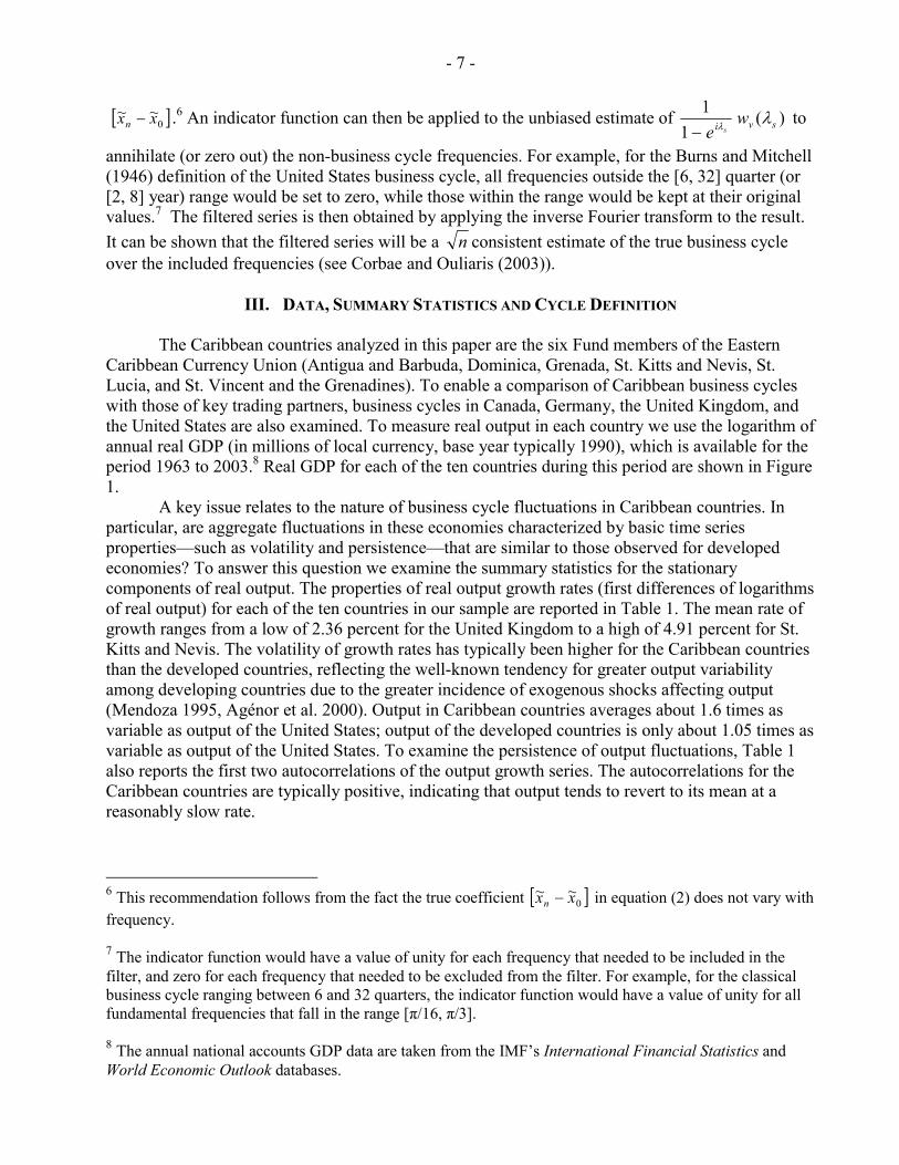
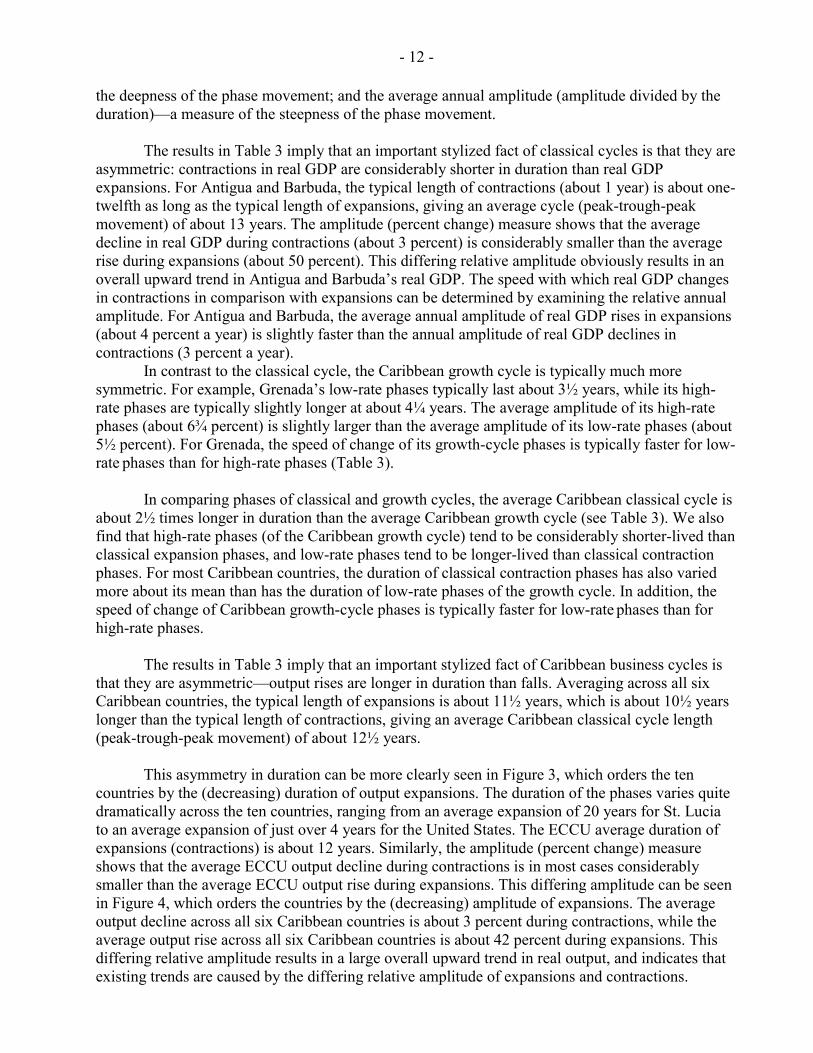
The results in Table 3 also imply that an important stylized fact that Caribbean growth cycles share with developed country growth cycles is that they are rather symmetric—positive deviations from trend output are of similar duration to negative deviations from trend output. Figures 5 and 6 present the duration and amplitude of high-rate and low-rate phases, again ordered by the decreasing duration and amplitude of high-rate phases, respectively. For the six Caribbean countries, the average duration of rises in trend-adjusted output in high-rate phases of growth cycles (about 2¾ years) is slightly longer than the average duration of declines in trend-adjusted output in low-rate phases (about 2½ years). Similarly, the average rise in trend-adjusted output in high-rate phases of growth cycles (about 5¾ percent) is slightly larger than the average fall in trend-adjusted output in low-rate phases (about 5¼ percent). Our results for classical and growth cycles in Caribbean output can be compared with those in the existing literature on developed-country and developing-country business cycles. While the length of the Caribbean classical cycle is longer than earlier findings on the duration of business cycles in developed countries (Baxter and King (1999)), the duration of Caribbean classical cycles is typically much longer than previously measured for developing-country business cycles. The mean duration of Caribbean classical cycles measured here (at between 2 and 12½ years) is longer than those derived by Rand and Tarp (2002) using the Bry-Boschan (1971) cycle-dating algorithm and quarterly output data for a range of middle-income developing countries. Rand and Tarp (2002) conclude that developing-country business cycles range in length between about 2 and 5 years; this contrasts with the accepted business cycle duration for the U.S. economy of between 2 and 8 years (Burns and Mitchell 1946). An implication of our results is that classical business cycles in Caribbean countries are much longer-lived than those of other (middle-income) developing countries, and generally slightly longer in duration than those of developed countries.14 According to the standard deviations of FD-filtered output, volatility in Caribbean countries is considerably higher than that of developed countries (Table 4). Caribbean output volatility ranges from St. Vincent and the Grenadines’ low of thirty percent greater than the United States, to St. Lucia’s high of over four times greater than that of the United States. On average, Caribbean output volatility is about 2.8 times greater than that of the United States. Using the largest of the ECCU economies (Antigua and Barbuda) as the base, Caribbean output volatility ranges from about half as variable (St. Vincent and the Grenadines) to thirty percent greater in variability (Dominica). In addition, the percentage of the sample period spent in a low-rate phase ranges from a low of 41 percent (Dominica, Grenada and St. Kitts and Nevis) to a high of 63 percent (United Kingdom).15
14 Canova (1999) finds that among many commonly used filters, frequency domain filters of the type used in this paper, applied to U.S. real GDP, are best able to replicate the properties of NBER growth cycles. He argues that such filters, due to their ability to extract both deterministic and stochastic trends from the data, are consistent with Pagan’s (1997) finding that a random walk with drift (without drift) is the best representation of the data-generating process that yields the typical duration and symmetry properties of the phases of classical (growth) cycles.
15 In contrast, the percentage of time Caribbean countries spent in contraction phase of the classical cycle was much smaller (Antigua and Barbuda 5 percent, Dominica 12, Grenada 7, St. Kitts and Nevis 5, St. Lucia 5, and St. Vincent and the Grenadines 5).

- 14 -
V. NONPARAMETRIC TESTS OF FEATURES OF CARIBBEAN BUSINESS CYCLES We also use some formal nonparametric tests to provide additional information on the nature
of the high-rate and low-rate phases in real GDP growth relative to trend. In particular, we use the Spearman rank correlation test, the Brain-Shapiro (1983) test of duration dependence, and Harding and Pagan’s (2002a) concordance statistic to examine whether there are similarities in the phases of Caribbean business cycles.16
A. Rank Correlation and Duration Dependence
Do Caribbean growth cycles have a similar ‘shape’? The Spearman rank correlation statistic provides a measure of whether there is a significant relationship between the severity (absolute amplitude) of high-rate phases and their duration, and the severity of low-rate phases and their duration. The null hypothesis of the Spearman rank correlation test is that there is no rank correlation between the amplitude of a high-rate phase (low-rate phase) and the duration of that high-rate phase (low-rate phase). Following Harding and Pagan (2002a), if we consider the duration and amplitude of a phase as two sides of a right-angled triangle, where the height of the triangle is the amplitude and the base of the triangle is the duration, then we can view this as a test of whether the phases of the growth cycle consistently have the same ‘shape’ (that is, the same angle of the hypotenuse).
We also examine whether there is any tendency for high-rate and low-rate phases of
deviation-from-trend growth in real GDP to maintain a fixed duration. If true, this would imply duration dependence—the longer any high-rate or low-rate phase continues, the more likely it is to switch to the other phase. Accordingly, we follow Diebold and Rudebusch (1992) and calculate the Brain-Shapiro statistic for duration dependence, which tests whether the probability of ending an high-rate or low-rate phase in a series is dependent on how long the series has been in that high-rate or low-rate phase. The null hypothesis of the Brain-Shapiro statistic is that the probability of exiting a phase is independent of the length of time a series has been in that phase. The two possible alternatives are that either: (i) the longer a high-rate or low-rate phase persists, the greater the likelihood that the phase will terminate (positive duration dependence); or (ii) the longer a high-rate or low-rate phase persists, the greater the likelihood that the phase will be self-perpetuating, and hence the lower the likelihood that the phase will terminate (negative duration dependence). The distribution of the Brain-Shapiro statistic is asymptotically N(0,1), which it quickly approaches even in small samples.17 The results of both the rank correlation and duration dependence tests are reported in Table 5.
For the growth cycle, the Spearman rank correlation statistic indicates that for half the
Caribbean countries (St. Kitts and Nevis, St. Lucia, and St. Vincent and the Grenadines) there is a relationship between the severity (absolute amplitude) of low-rate phases and their duration, and so there is some evidence of a consistent shape to low-rate phases. Apart from Antigua and Barbuda, this feature is not found for high-rate phases of the growth cycle.
16 Unfortunately, the limited number of completed classical cycles for Caribbean countries and several developed countries precluded use of the rank correlation and Brain-Shapiro statistics.
17 A negative (positive) Brain-Shapiro statistic is associated with positive (negative) duration dependence (see Diebold and Rudebusch (1992)).

- 15 -
For most Caribbean countries, the Brain-Shapiro statistic indicates that probability of a low-
rate or high-rate phase of real GDP growth ending is independent of its duration. That is, for most Caribbean countries there is no evidence from past history that the duration of positive (negative) output gaps increases the probability of switching to a low-rate (high-rate) phase. However, for Dominica the negative duration dependence in low-rate phases (given the significantly positive Brain-Shapiro statistic) indicates that the longer low-rate phases of real GDP growth continued, the lower was the probability of switching to a high-rate phase. Similarly, the negative duration dependence in high-rate phases of the St. Vincent and the Grenadines growth cycle indicates that the termination probability of its high-rate phases shrank the longer the phase lasted.
B. Correlation and Concordance Statistics Comovement in Real GDP (Classical Cycles)
We are interested in the question as to whether expansions and contractions in the level of real GDP move together, both among Caribbean countries and between individual Caribbean countries and non-Caribbean countries. That is, we are interested whether the turning points in classical business cycles are similar across countries. To analyze this question we use two measures of comovement: the correlation of growth rates of real output, and the concordance between real output series.
The correlation matrix is presented in Table 6.18 Many of the country pairs are significant at the five percent level or greater. On this basis, there appears to be evidence that the real output series of three of the six Caribbean countries tend to comove with cycles in Canadian output. For two of the Caribbean countries (Antigua and Barbuda and Grenada), output appears to comove with cycles in U.S. output. The results suggest that the level of activity in industrial countries typically has a positive, yet often weak association with Caribbean output. Among the Caribbean islands, comovement in real output appears strongest between St. Vincent and the Grenadines and St. Lucia, with Antigua and Barbuda and Grenada, Dominica and St. Vincent and the Grenadines, St. Lucia and St. Kitts and Nevis also displaying evidence of synchronized output.
Most previous analyses have used correlation statistics as their measure of comovement of economic time series. However, bivariate correlation measures are based on covariance, which is affected by amplitude changes (shifts in the level of the two series) as well as by the fraction of time that any two series are rising together and falling together. It is possible for a large, one-time shift in the level of two series (for example, those induced by the oil shock of 1974) to induce significant correlation in otherwise unrelated series. In contrast, such a shock will only be important under a concordance test to the extent that the comovement lasts for a lengthy period of time. McDermott and Scott (2000) demonstrate that the covariance of two series may be dominated by the amplitude
18 The output correlations reported are contemporaneous correlations. We also examined leads and lags in the relationship between output growth, yet found that for most countries the correlations peak at or near lag zero, suggesting that output fluctuations are transmitted fairly quickly (within one year) across countries.

- 16 -
of a particularly long swing which is common to both series.19 Accordingly, it may be more relevant to know the degree of synchronization of national business cycles, and so examine the proportion of time that two output series are expanding together and contracting together.
For this purpose, we make use of the concordance statistic originally proposed by Harding and Pagan (2002a). Concordance is measured by a simple non-parametric statistic that describes the proportion of time two series, ix and jx , are in the same phase (Harding and Pagan 2002a, 2002b). Specifically, let { Si,t } be a series taking the value unity when the series ix (real GDP in country i) is in an expansion state, and zero when it is in a contraction state; and let { Sj,t } be a series taking the value unity when the series jx (real GDP in country j) is in an expansion state, and zero when it is in a contraction state. The degree of concordance is then
( ) ( ) ( ){ },1.1
1 1 ,,,,1 ∑ ∑= =− −−+⋅=
T
t
T
t tjtitjtiij SSSSTC (3) where Si and Sj are as defined above, T is the sample size and Cij measure the proportion of time the two series are in the same state. To interpret Cij, a value of say 0.7 for the index indicates that ix and jx are in the same phase (that is, expanding or contracting together) 70 percent of the time. The series ix is exactly pro-cyclical (counter-cyclical) with jx if Cij = 1 (Cij = 0).
As a proportion, the values that Cij may take are clearly bounded between zero and one. Faced with a realized concordance index of, for example, 0.7, it is natural to assume that this is large relative to zero. However, even for two unrelated series the expected value of the concordance index may be 0.5 or higher. For example, consider the case of two fair coins being tossed. The probability that both coins are in the same phase—that is, both heads or both tails—is 0.5.
More generally, a disadvantage of Cij is that it does not provide a means of determining if
the extent of comovement (or synchronization) between cycles in the two series is statistically significant. To do so we need a concordance test statistic. If the expected value of Cij is evaluated under the assumption of mean independence, then, following Harding and Pagan (2002b), the t-statistics examining the null hypothesis of no concordance between the two series can be computed from the regression coefficient estimate attached to Si,t in the regression of Sj,t against a constant term and Si,t .20 21
19 McDermott and Scott (2000) consider an example with two independent random walks of 100 observations each, with variances chosen so as to generate series that look like ‘typical’ economic time series. A jump point is added halfway through both series. As expected, the concordance index measures 0.5. However, the correlation of the first-differenced series is large and significant, even though the two series are otherwise random. This result reflects the fact that correlation, as scaled covariance, mixes the concepts of duration and amplitude into one measure. The correlation statistic is therefore not easily interpreted—a high number may be the result of significant comovement through time, or, as here, the result of a single large event that is common to the two series. 20 In addition, given that the errors from such a regression are unlikely to be i.i.d., due to the strong likelihood of serial correlation or heteroscedasticity in Si,t , the t-ratio for the regression coefficient has been made robust to higher-order serial correlation and heteroscedasticity. Positive serial correlation in Si,t biases hypothesis tests toward rejecting the null of no concordance (see Harding and Pagan 2002b).

- 17 -
The results of the concordance statistic (shown in Table 7) reveal that the association
between real GDP within the ECCU countries and between developed country–ECCU country pairs appears to be very strong. For example, real output in Canada and Antigua and Barbuda are highly synchronized—they move in the direction 93 percent of the time. This suggests that real output in these 10 countries spends much of the time in the same phase of the classical cycle. However, the pairwise correlations of phase states are typically rather small (and often negative), which suggests that it is the very high values of the mean value of Si , rather than a strong correlation between phase states, which underpins the high measured value of concordance (see the bottom row of Table 7). That is, the fact that most countries spend a very large proportion of the sample in an expansion phase has biased upward the measured value of concordance. This effect is important for Canada, which has a mean value of its phase state indicator of 0.93 and shows concordance with the Caribbean economies in the range of 0.80 to 0.93, yet only shows correlations of phase states with Caribbean economies in the range of -0.10 to 0.37. Once the concordance statistic is mean corrected (which is essentially what occurs when using the correlation of phase states), there is only evidence of significant synchronization of classical cycles (involving rejection of the null hypothesis of no concordance) for the United Kingdom and the United States, which are in the same state of the classical cycle 95 percent of the time. This result highlights the need to use hypothesis testing procedures rather than relying on point estimates of concordance. In summary, evidence for the null hypothesis of no association between the classical cycles of the ten countries is quite strong.
Comovement in Real GDP Deviations from Trend (Growth Cycles)
Similarly, we may be interested in the question as to whether output deviations from trend move with each other—that is, how synchronized across countries are output gaps? To analyze this question we follow Scott (2000) and examine the cross-correlation and concordance statistics for filtered output.
The correlation matrix presented in Table 8 looks at the cross-correlation of FD-filtered
output in one country and a similarly-transformed output series for another country. On this basis, there appears to be strong evidence that filtered output (output gap) series of all but two of the six Caribbean countries tend to comove with cycles in Canadian filtered output. In contrast, there is no evidence that output gaps in Caribbean countries comove with either the United States or United Kingdom output gaps. Among the Caribbean islands, comovement in filtered output appears strongest between St. Lucia and St. Kitts and Nevis, with Antigua and Barbuda and Grenada, and St. Lucia and Grenada also having evidence of synchronized output gaps.
As previously, we also use the concordance statistic to examine whether Caribbean
economies are above or below potential at the same time or not. Here the formula for the concordance statistic is as given above in equation (3), with { Si,t } a series taking the value unity when the series ix (deviation of output from trend in country i) is in a high-rate phase, and zero when it is in a low-rate phase; and { Sj,t } a series taking the value unity when the series jx (deviation of output from trend in country j) is in a high-rate phase, and zero when it is in a low-rate phase.
21 See also Cashin and McDermott (2002) and Artis et al. (2002) for earlier uses of the concordance statistic to examine comovement of cycles in economic time series.

- 18 -
The concordance results examining the synchronization of output gaps are given in Table 9.
There is strong evidence of an association between the growth cycles of Canada and Grenada and Canada and St. Kitts and Nevis, which expand (and contract) together 66 percent of the time. Importantly, while the United States and the United Kingdom have synchronized growth cycles, there is little evidence of synchronization between the growth cycles of the United States and the Caribbean, or the growth cycles of the United Kingdom and the Caribbean. Among the Caribbean islands, evidence of comovement in growth cycles appears strongest for the pairs Antigua and Barbuda and Dominica, Grenada and St. Kitts and Nevis, and St. Lucia and St. Vincent and the Grenadines. Interestingly, growth cycles in Antigua and Barbuda and St. Vincent and the Grenadines are countercyclical, in that they move together only 34 percent of the time.
Caribbean Links with Industrial Country Business Cycles
In this section we examine further the relationship between output (GDP) fluctuations in each of j industrial countries (yj,t) and output in each of i ECCU countries (xi,t). The degree of comovement of output series is measured by the magnitude of the cross-correlation coefficients at (annual) lag k, ρ(k), where k ∈ {0, ±1, ±2, ±3}. These correlations (as reported in Table 10) are between the stationary components of the output series (yt and xt), with both components derived using the FD filter. The cross-correlation indexes indicate the shift in time of xt+k (the cycle in Caribbean country output) in comparison with yt (the cycle in industrial country output). In line with the existing literature, we say that xt leads the industrial output cycle (that is, xi,t+k leads yj,t) by k periods (years) if |ρ(k)| is maximum for a negative k; the Caribbean output cycle is synchronous with the industrial country output cycle (that is, xi,t+k is synchronized with yj,t) if |ρ(k)| is maximum for k = 0; and the Caribbean output cycle lags the industrial country output cycle (that is, xi,t+k lags yj,t) by k periods (years) if |ρ(k)| is maximum for a positive k.22 Possible shifts (leads and lags) in the cyclical movements of each series are identified by how early or late with respect to the contemporaneous period the highest statistically significant correlation occurs.
Business cycle fluctuations in Caribbean countries tend to be correlated with cycles in
industrial country output. As reported in Table 6, the contemporaneous correlations between industrial country output and Caribbean output are positive for a majority of Caribbean countries. However, there is little evidence of Caribbean output being correlated with either United States or United Kingdom cycles, even when allowing for leads and lags in cycles (Table 10). Germany’s output is positively contemporaneously correlated with Grenada, with some indication that German output appears to have a negative effect on Grenada (and St. Lucia) output with a lag of about two years.
Consistent with the earlier results, the strongest business cycles links are between Canadian
output and Caribbean output. Canadian output appears to have a positive (synchronous) effect on the output of four of the six Caribbean countries at or near lag zero, suggesting that Canadian output fluctuations are transmitted fairly rapidly to Caribbean countries (Table 10).
Another measure of the comovement of growth cycles is given by the magnitude of the
concordance index at (annual) lag k, Cij(k), where k ∈ {0, ±1, ±2, ±3} and concordance measures 22 For an earlier study which examines bivariate correlations in detrended macroeconomic time series, see Agénor, McDermott and Prasad (2000).

- 19 -
the proportion of time that Si,t , the phase indicator of series i (the real output of country i), and Sj,t , the phase indicator of series j (the real output of country j), move in the same direction. In particular, the cross-concordance indexes Cij(k) indicate the shift in time of Sj,t+k (the cycle in real output of country i) in comparison with Si,t (the cycle in real output of country j). In line with the results of Table 9, which examined contemporaneous concordance among country pairs, no significant concordance is found between Caribbean countries and United States or United Kingdom growth cycles, at any lead or lag. There is strong evidence of synchronized (contemporaneous) growth cycles between Canada and St. Kitts and Nevis and Canada and Grenada, and evidence of an association between Canadian growth cycles and the growth cycles of Antigua and Barbuda and St. Lucia (both with a lag of three years). There is also some evidence of an association between German growth cycles and the St. Lucian growth cycle (lagged one year). In summary, the null hypothesis of no association between the Canadian growth cycle and Caribbean growth cycles is strongly rejected for four of the six Caribbean countries—the null is never rejected for the Caribbean-United States and Caribbean-United Kingdom cyclical relationship. Clearly, links between the business cycles of Canada and the Caribbean are the strongest among the developed countries examined in this study.23
VI. CONCLUSION The relative mildness of economic fluctuations in many developed economies since the
1950s, in tandem with recent developments in time series analysis, has led to a renewed interest in growth cycles (cyclical movements in trend-adjusted output) in comparison with classical cycles (cyclical movements in trend-unadjusted output). In this study we have examined the key stylized facts of Caribbean business cycles over the period 1963-2003, and calculated a chronology for the classical cycle (involving expansions and contractions in the level of real output) and the growth cycle (involving alternating periods of above- and below-trend economic growth). In obtaining new measures of classical and growth cycles, we applied simple rules to date turning points in the classical business cycle, and used a recently developed frequency domain filter to estimate the growth cycle.
In examining the stylized features of Caribbean business cycles, we have several key findings. First, Caribbean growth cycles are relatively symmetric in both duration and amplitude. This is unlike the Caribbean classical cycle, which typically exhibits long-lived expansions and much shorter-lived contractions, and much greater amplitude of output movement in expansions than contractions. Second, for about half the Caribbean countries there is evidence of a relationship between below-trend movements in real GDP and their duration; for all but one of the Caribbean countries there is no evidence of a similar relationship for above-trend movements in real GDP. Third, for most Caribbean countries there is little evidence that either below- or above-trend phases in real GDP growth are duration dependent. Accordingly, while there are some similarities in the ups and downs of Caribbean growth cycles, no two business cycles are exactly alike. Fourth, while movements in the Canadian classical cycle appear to be reasonably synchronized with movements
23 There are several important links between Canada and the countries of the Eastern Caribbean. First, Canada is a major provider of bilateral overseas development assistance flows to the countries of the Eastern Caribbean (OECD (2004)). Second, Canadian-licensed banks are active in all ECCU countries. Third, Canada has traditionally been an important emigrant destination for Caribbean nationals, and accounts for a large share of remittance flows into the Caribbean.

- 20 -
in the classical cycle of Caribbean countries, there is less synchronization of Caribbean movements in real output with those of the United States and the United Kingdom. Fifth, there is little synchronization of Caribbean output deviations from trend (growth cycles) with growth cycles of the United States and the United Kingdom, and some comovement between Canadian and Caribbean growth cycles. While there is some evidence of synchronization among the classical business cycles of Caribbean countries, there is stronger evidence of synchronization of Caribbean growth cycles.

- 21 -
Table 1. Properties of Output Growth Rates, 1963-2003
Mean (percentage)
Standard deviation
(percentage)
Coefficient of variation
Autocorrelation coefficient
(1 year) (2 years)
Canada (CAN) 3.86 2.21 0.57 0.32 0.10 Germany (GER) 2.70 2.60 0.96 0.33 -0.13 United Kingdom (UNK) 2.36 1.90 0.81 0.29 -0.19 United States of America (USA) 3.20 2.10 0.66 0.22 -0.19 Antigua and Barbuda (ATG) 4.70 2.79 0.59 0.23 0.01 Dominica (DMA) 3.54 5.11 1.44 -0.11 0.07 Grenada (GRD) 4.38 2.88 0.66 0.43 0.08 St. Kitts and Nevis (KNA) 4.91 2.42 0.49 0.12 0.15 St. Lucia (LCA) 4.41 4.21 0.95 0.38 0.32 St. Vincent and the Grenadines (VCT) 4.25 3.14 0.74 -0.14 0.23
Sources: Author’s calculations. Notes: Sample moments were computed from log-differences of real output. Coefficient of variation is the ratio of the standard deviation to the arithmetic mean. Autocorrelations of one and two years are the first- and second-order autocorrelation coefficients, respectively.
Table 2. Summary Statistics for Filtered Output, 1963-2003
HP Standard deviation
HP Skewness
HP Kurtosis
FD Standard deviation
FD Skewness
FD Kurtosis
FD Business cycle
frequency (years)
CAN 2.18 -0.53 -0.06 2.14 -0.42 -0.55 [2, 9] GER 2.58 0.71 0.91 2.13 0.47 0.49 [2, 9] UNK 2.03 0.42 0.64 1.38 0.91 2.22 [2, 8] USA 2.04 -0.42 -0.22 1.16 0.22 0.54 [2, 6] ATG 2.81 -0.45 0.47 2.88 -0.55 0.04 [2, 13] DMA 3.66 -1.20 4.90 3.75 -1.22 4.82 [2, 11] GRD 3.28 0.15 -0.65 2.64 0.55 0.62 [2, 9] KNA 2.26 -0.40 2.50 3.34 -0.76 0.75 [2, 15] LCA 3.99 -0.04 -0.11 5.14 -0.18 -0.46 [2, 20] VCT 2.55 0.30 -0.40 1.53 -0.25 0.08 [2, 7]
Sources: Author’s calculations. Notes: HP denotes the Hodrick–Prescott (1980) filtered output (with smoothing parameter λ=100); FD denotes the Corbae–Ouliaris (2003) filtered output. The business cycle frequencies used to derive FD-filtered output are given in the last column of the table, and were determined using the rule set out in Section III.A—for annual data, minimum cycle length is 2 years while the upper bound on cycle length is the average duration of each country’s classical business cycle (see Table 3). The skewness measure is µ3/(µ2)1.5 and the kurtosis measure is µ4/(µ2)2 – 3, where µr is the rth (central) moment. The skewness of a symmetrical distribution, such as the normal, is zero; similarly, the kurtosis (as previously defined) of the normal distribution is zero.

- 22 -
Table 3.A. Duration and Amplitude of Phases, Antigua and Barbuda Business Cycles, 1963-2003
Antigua and Barbuda Classical Cycles Turning Duration Amplitude Annual Turning Duration Amplitude Annual Duration of Point Date Amplitude Point Date Amplitude Classical Cycle (year) (year) (P to P) (T to T) Peak Trough Trough Peak (P) (T) (T) (P) (1) (2) (3) (4) (5) (6) (7) (8) (9) (10) (11) (12)
Contraction Phase ______ Expansion Phase __ _______ 1981 1982 1 -0.95 -0.95 1982 1994 12 49.66 4.14 1994 1995 1 -4.94 -4.94 1995 13 13 Average 1.00 -2.95 -2.95 12.00 49.66 4.14 13 13 Std. Deviation 0 2.82 2.82 … … … … … Coeff. of Variation 0 0.96 0.96 … … … … …
Antigua and Barbuda Growth Cycles Turning Duration Amplitude Annual Turning Duration Amplitude Annual Duration of Point Date Amplitude Point Date Amplitude Growth Cycle (year) (year) (D to D) (U to U) Downturn Upturn Upturn Downturn (D) (U) (U) (D) (1) (2) (3) (4) (5) (6) (7) (8) (9) (10) (11) (12)
Low-rate Phase ________ High-rate Phase __ ________ 1967 1969 2 1.80 0.90 3 1969 1970 1 -1.61 -1.61 1970 1974 4 6.54 1.63 3 1974 1978 4 -4.97 -1.24 1978 1980 2 3.64 1.82 5 8 1980 1983 3 -8.29 -2.76 1983 1989 6 10.67 1.78 6 5 1989 1992 3 -7.73 -2.58 1992 1994 2 3.82 1.91 9 9 1994 1995 1 -7.75 -7.75 1995 2000 5 9.96 1.99 5 3 Average 2.40 -6.07 -3.19 3.50 6.07 1.67 6.25 5.60 Std. Deviation 1.34 2.81 2.63 1.76 3.63 0.40 1.89 2.79 Coeff. of Variation 0.56 0.46 0.82 0.50 0.60 0.24 0.30 0.50 Source: Author’s calculations. Notes: For each of the two cycles (classical and growth), and for each of two phases (expansion and contraction for the classical cycle; high-rate and low-rate for the growth cycle), five results are presented. First, the dates of each peak-to-trough (downturn-to-upturn) movement and trough-to-peak (upturn-to-downturn) movement. Second, the duration (in years) of each phase. Third, the amplitude of the aggregate phase movement in output (in percent change) for each phase. Fourth, the annual amplitude (amplitude divided by the duration) for each phase. Fifth, the average duration (in years) of each cycle.

- 23 -
Table 3.B. Duration and Amplitude of Phases, Dominica Business Cycles, 1963-2003
Dominica Classical Cycles Turning Duration Amplitude Annual Turning Duration Amplitude Annual Duration of Point Date Amplitude Point Date Amplitude Classical Cycle (year) (year) (P to P) (T to T) Peak Trough Trough Peak (P) (T) (T) (P) (1) (2) (3) (4) (5) (6) (7) (8) (9) (10) (11) (12)
Contraction Phase ______ Expansion Phase __ _______ 1978 1979 1 -17.09 -17.09 1979 1988 9 44.89 4.99 1988 1989 1 -1.14 -1.14 1989 2000 11 23.85 2.17 10 10 2000 12 Average 1.00 -9.12 -9.12 10.00 34.37 3.58 11.00 10.00 Std. Deviation 0 11.28 11.28 1.41 14.88 1.99 1.41 … Coeff. of Variation 0 1.23 1.23 1.41 0.43 0.56 0.13 …
Dominica Growth Cycles Turning Duration Amplitude Annual Turning Duration Amplitude Annual Duration of Point Date Amplitude Point Date Amplitude Growth Cycle (year) (year) (D to D) (U to U) Downturn Upturn Upturn Downturn (D) (U) (U) (D) (1) (2) (3) (4) (5) (6) (7) (8) (9) (10) (11) (12)
Low-rate Phase ________ High-rate Phase __ ________ 1965 1967 2 -1.81 -0.90 1967 1969 2 1.89 0.95 1969 1970 1 -2.01 -2.01 1970 1974 4 4.75 1.19 4 3 1974 1977 3 -3.07 -1.02 1977 1978 1 7.48 7.48 5 7 1978 1979 1 -20.10 -20.10 1979 1982 3 14.81 4.94 4 2 1982 1983 1 -1.08 -1.08 1983 1984 1 0.84 0.84 4 4 1984 1985 1 -1.56 -1.56 1985 1988 3 5.12 1.71 2 2 1988 1989 1 -5.84 -5.84 1989 1990 1 1.55 1.55 4 4 1990 1994 4 -3.84 -0.96 1994 2000 6 9.47 1.58 2 5 Average 1.75 -4.91 -4.18 2.63 5.74 2.53 3.57 3.86 Std. Deviation 1.16 6.33 6.64 1.77 4.74 2.39 1.13 1.77 Coeff. of Variation 0.67 1.29 1.59 0.67 0.83 0.94 0.32 0.46 Source: Author’s calculations. Notes: For each of the two cycles (classical and growth), and for each of two phases (expansion and contraction for the classical cycle; high-rate and low-rate for the growth cycle), five results are presented. First, the dates of each peak-to-trough (downturn-to-upturn) movement and trough-to-peak (upturn-to-downturn) movement. Second, the duration (in years) of each phase. Third, the amplitude of the aggregate phase movement in output (in percent change) for each phase. Fourth, the annual amplitude (amplitude divided by the duration) for each phase. Fifth, the average duration (in years) of each cycle.

- 24 -
Table 3.C. Duration and Amplitude of Phases, Grenada Business Cycles, 1963-2003
Grenada Classical Cycles Turning Duration Amplitude Annual Turning Duration Amplitude Annual Duration of Point Date Amplitude Point Date Amplitude Classical Cycle (year) (year) (P to P) (T to T) Peak Trough Trough Peak (P) (T) (T) (P) (1) (2) (3) (4) (5) (6) (7) (8) (9) (10) (11) (12)
Contraction Phase ______ Expansion Phase __ _______ 1992 1993 1 -1.40 -1.40 1993 2000 7 28.72 4.10 2000 2002 2 -3.61 -1.80 2002 8 9 Average 1.50 -2.50 -1.60 7.00 28.72 4.10 8.00 9.00 Std. Deviation 0.71 1.56 0.28 … … … … … Coeff. of Variation 0.47 0.62 0.18 … … … … …
Grenada Growth Cycles Turning Duration Amplitude Annual Turning Duration Amplitude Annual Duration of Point Date Amplitude Point Date Amplitude Growth Cycle (year) (year) (D to D) (U to U) Downturn Upturn Upturn Downturn (D) (U) (U) (D) (1) (2) (3) (4) (5) (6) (7) (8) (9) (10) (11) (12)
Low-rate Phase ________ High-rate Phase __ ________ 1969 1975 6 -6.89 -1.15 1975 1979 4 7.85 1.96 1979 1984 5 -7.14 -1.43 1984 1987 3 6.58 2.19 10 9 1987 1988 1 -2.97 -2.97 1988 1991 3 2.12 0.71 8 4 1991 1993 2 -5.43 -2.71 1993 2000 7 10.41 1.49 4 5 Average 3.50 -5.61 -2.07 4.25 6.74 1.59 7.33 6.00 Std. Deviation 2.38 1.91 0.91 1.89 3.47 0.65 3.06 2.65 Coeff. of Variation 0.68 0.34 0.44 0.45 0.51 0.41 0.42 0.44 Source: Author’s calculations. Notes: For each of the two cycles (classical and growth), and for each of two phases (expansion and contraction for the classical cycle; high-rate and low-rate for the growth cycle), five results are presented. First, the dates of each peak-to-trough (downturn-to-upturn) movement and trough-to-peak (upturn-to-downturn) movement. Second, the duration (in years) of each phase. Third, the amplitude of the aggregate phase movement in output (in percent change) for each phase. Fourth, the annual amplitude (amplitude divided by the duration) for each phase. Fifth, the average duration (in years) of each cycle.

- 25 -
Table 3.D. Duration and Amplitude of Phases, St. Kitts and Nevis Business Cycles, 1963-2003
St. Kitts and Nevis Classical Cycles Turning Duration Amplitude Annual Turning Duration Amplitude Annual Duration of Point Date Amplitude Point Date Amplitude Classical Cycle (year) (year) (P to P) (T to T) Peak Trough Trough Peak (P) (T) (T) (P) (1) (2) (3) (4) (5) (6) (7) (8) (9) (10) (11) (12)
Contraction Phase ______ Expansion Phase __ _______ 1982 1983 1 -2.25 -2.25 1983 1997 14 56.25 4.02 1997 1998 1 -0.20 -0.20 1998 15 15 Average 1.00 -1.23 -1.23 14.00 56.25 4.02 15.00 15.00 Std. Deviation 0 1.45 1.45 … … … … … Coeff. of Variation 0 1.18 1.18 … … … … …
St. Kitts and Nevis Growth Cycles Turning Duration Amplitude Annual Turning Duration Amplitude Annual Duration of Point Date Amplitude Point Date Amplitude Growth Cycle (year) (year) (D to D) (U to U) Downturn Upturn Upturn Downturn (D) (U) (U) (D) (1) (2) (3) (4) (5) (6) (7) (8) (9) (10) (11) (12)
Low-rate Phase ________ High-rate Phase __ ________ 1971 1975 4 -4.08 -1.02 1975 1977 2 0.78 0.39 1977 1978 1 -1.99 -1.99 1978 1980 2 2.02 1.01 6 3 1980 1983 3 -9.69 -3.23 1983 1989 6 14.41 2.40 3 5 1989 1992 3 -6.20 -2.07 1992 1994 2 1.21 0.60 9 9 1994 1995 1 -1.12 -1.12 1995 1997 2 3.91 1.96 5 3 1997 1999 2 -3.81 -1.91 1999 2000 1 1.76 1.76 3 4 Average 2.33 -4.48 -1.89 2.50 4.02 1.35 5.20 4.80 Std. Deviation 1.21 3.10 0.80 1.76 5.21 0.81 2.49 2.49 Coeff. of Variation 0.52 0.69 0.42 0.70 1.30 0.60 0.48 0.52 Source: Author’s calculations. Notes: For each of the two cycles (classical and growth), and for each of two phases (expansion and contraction for the classical cycle; high-rate and low-rate for the growth cycle), five results are presented. First, the dates of each peak-to-trough (downturn-to-upturn) movement and trough-to-peak (upturn-to-downturn) movement. Second, the duration (in years) of each phase. Third, the amplitude of the aggregate phase movement in output (in percent change) for each phase. Fourth, the annual amplitude (amplitude divided by the duration) for each phase. Fifth, the average duration (in years) of each cycle.

- 26 -
Table 3.E. Duration and Amplitude of Phases, St. Lucia Business Cycles, 1963-2003
St. Lucia Classical Cycles Turning Duration Amplitude Annual Turning Duration Amplitude Annual Duration of Point Date Amplitude Point Date Amplitude Classical Cycle (year) (year) (P to P) (T to T) Peak Trough Trough Peak (P) (T) (T) (P) (1) (2) (3) (4) (5) (6) (7) (8) (9) (10) (11) (12)
Contraction Phase ______ Expansion Phase __ _______ 1979 1980 1 -0.43 -0.43 1980 2000 20 59.78 2.99 2000 2001 1 -4.57 -4.57 21 21 Average 1.00 -2.50 -2.50 20.00 59.78 2.99 21.00 21.00 Std. Deviation 0 2.93 2.93 … … … … … Coeff. of Variation 0 1.17 1.17 … … … … …
St. Lucia Growth Cycles Turning Duration Amplitude Annual Turning Duration Amplitude Annual Duration of Point Date Amplitude Point Date Amplitude Growth Cycle (year) (year) (D to D) (U to U) Downturn Upturn Upturn Downturn (D) (U) (U) (D) (1) (2) (3) (4) (5) (6) (7) (8) (9) (10) (11) (12)
Low-rate Phase ________ High-rate Phase __ ________ 1967 1968 1 -1.65 -1.65 1968 1971 3 3.14 1.05 1971 1975 4 -8.39 -2.10 1975 1978 3 14.22 4.74 4 7 1978 1984 6 -19.04 -3.17 1984 1986 2 8.86 4.43 7 9 1986 1987 1 -4.12 -4.12 1987 1990 3 12.56 4.19 8 3 1990 1991 1 -4.22 -4.22 1991 1992 1 3.19 3.19 4 4 1992 1997 5 -6.60 -1.32 2 6 Average 3.00 -7.34 -2.76 2.40 8.39 3.52 5.00 5.80 Std. Deviation 2.28 6.18 1.26 0.89 5.15 1.50 2.45 2.39 Coeff. of Variation 0.76 0.84 0.45 0.37 0.61 0.43 0.49 0.41 Source: Author’s calculations. Notes: For each of the two cycles (classical and growth), and for each of two phases (expansion and contraction for the classical cycle; high-rate and low-rate for the growth cycle), five results are presented. First, the dates of each peak-to-trough (downturn-to-upturn) movement and trough-to-peak (upturn-to-downturn) movement. Second, the duration (in years) of each phase. Third, the amplitude of the aggregate phase movement in output (in percent change) for each phase. Fourth, the annual amplitude (amplitude divided by the duration) for each phase. Fifth, the average duration (in years) of each cycle.

- 27 -
Table 3.F. Duration and Amplitude of Phases, St. Vincent and the Grenadines Business Cycles, 1963-2003
St. Vincent and the Grenadines Classical Cycles Turning Duration Amplitude Annual Turning Duration Amplitude Annual Duration of Point Date Amplitude Point Date Amplitude Classical Cycle (year) (year) (P to P) (T to T) Peak Trough Trough Peak (P) (T) (T) (P) (1) (2) (3) (4) (5) (6) (7) (8) (9) (10) (11) (12)
Contraction Phase ______ Expansion Phase __ _______ 1993 1994 1 -3.00 -3.00 1994 2000 6 20.88 3.48 2000 2001 1 -0.16 -0.16 7 7 Average 1.00 -1.58 -1.58 6.00 20.88 3.48 7.00 7.00 Std. Deviation 0 2.01 2.01 … … … … … Coeff. of Variation 0 1.27 1.27 … … … … …
St. Vincent and the Grenadines Growth Cycles Turning Duration Amplitude Annual Turning Duration Amplitude Annual Duration of Point Date Amplitude Point Date Amplitude Growth Cycle (year) (year) (D to D) (U to U) Downturn Upturn Upturn Downturn (D) (U) (U) (D) (1) (2) (3) (4) (5) (6) (7) (8) (9) (10) (11) (12)
Low-rate Phase ________ High-rate Phase __ ________ 1966 1968 2 -3.37 -1.69 1968 1971 3 4.16 1.39 1971 1973 2 -2.97 -1.48 1973 1974 1 0.80 0.80 5 5 1974 1975 1 -0.92 -0.92 1975 1976 1 2.93 2.93 3 2 1976 1977 1 -3.65 -3.65 1977 1978 1 5.10 5.10 2 2 1978 1980 2 -5.64 -2.82 1980 1981 1 3.25 3.25 2 3 1981 1983 2 -1.06 -0.53 1983 1984 1 1.94 1.94 3 3 1984 1987 3 -4.79 -1.60 1987 1988 1 6.10 6.10 3 4 1988 1989 1 -3.61 -3.61 1989 1990 1 1.13 1.13 4 2 1990 1991 1 -2.44 -2.44 1991 1992 1 3.93 3.93 2 2 1992 1994 2 -5.31 -2.66 1994 1995 1 5.13 5.13 2 3 1995 1997 2 -2.85 -1.42 1997 1999 2 2.03 1.01 3 3 1999 2001 2 -2.02 -1.01 2001 4 4 Average 1.75 -3.22 -1.99 1.27 3.32 2.97 3.00 3.00 Std. Deviation 0.62 1.52 1.04 0.65 1.74 1.88 1.00 1.00 Coeff. of Variation 0.36 0.47 0.52 0.51 0.52 0.63 0.33 0.33 Source: Author’s calculations. Notes: For each of the two cycles (classical and growth), and for each of two phases (expansion and contraction for the classical cycle; high-rate and low-rate for the growth cycle), five results are presented. First, the dates of each peak-to-trough (downturn-to-upturn) movement and trough-to-peak (upturn-to-downturn) movement. Second, the duration (in years) of each phase. Third, the amplitude of the aggregate phase movement in output (in percent change) for each phase. Fourth, the annual amplitude (amplitude divided by the duration) for each phase. Fifth, the average duration (in years) of each cycle.

- 28 -
Tabl
e 4.
Fea
ture
s of G
row
th C
ycle
s, FD
-filt
ered
Rea
l GD
P, 1
963-
2003
CA
N
GE
R
UN
K
USA
A
TG
D
MA
G
RD
K
NA
L
CA
V
CT
N
umbe
r of d
ownt
urns
7
6 6
8 5
8 4
6 6
12
Num
ber o
f upt
urns
7
6 6
9 6
8 4
6 5
11
Tim
e sp
ent i
n lo
w-r
ate
phas
e (p
erce
nt)
46
49
63
54
49
41
41
41
44
51
Ave
rage
dur
atio
n of
hig
h-ra
te p
hase
(yea
rs)
2.57
3.
00
2.17
2.
11
3.50
2.
63
4.25
2.
50
2.40
1.
27
Ave
rage
dur
atio
n of
low
-rat
e ph
ase
(yea
rs)
2.29
2.
83
2.83
2.
00
2.40
1.
75
3.50
2.
33
3.00
1.
75
Ave
rage
am
plitu
de o
f hig
h-ra
te p
hase
(per
cent
cha
nge)
3.
19
4.78
3.
34
2.67
6.
07
5.74
6.
74
4.01
8.
39
3.32
A
vera
ge a
mpl
itude
of l
ow-r
ate
phas
e (p
erce
nt c
hang
e)
-3.3
9 -4
.70
-3.3
6 -2
.84
-6.0
7 -4
.91
-5.6
1 -4
.48
-7.3
4 -3
.22
V
olat
ility
(sta
ndar
d de
viat
ion
of g
row
th c
ycle
) 2.
14
2.13
1.
38
1.62
2.
88
3.75
2.
64
3.34
5.
14
1.53
R
atio
of v
olat
ility
to U
SA v
olat
ility
1.
84
1.84
1.
19
1.00
2.
48
3.23
2.
27
2.87
4.
42
1.32
R
atio
of v
olat
ility
to A
TG v
olat
ility
0.
74
0.74
0.
48
0.40
1.
00
1.30
0.
92
1.16
1.
79
0.53
So
urce
s: A
utho
r’s c
alcu
latio
ns.
N
otes
: FD
den
otes
the
Cor
bae–
Oul
iaris
(200
3) fi
ltere
d G
DP
serie
s.

- 29 -
Tabl
e 5.
Non
para
met
ric T
ests
: Con
tract
ions
/Exp
ansi
ons i
n R
eal G
DP
Gro
wth
, 196
3-20
03
R
eal G
DP
Gro
wth
Low
-rate
Pha
se
H
igh-
rate
Pha
se
-
Num
ber o
f Pha
ses
B
rain
-Sha
piro
Spe
arm
an
Bra
in-S
hapi
ro
Spe
arm
an
Low
-rate
H
igh-
rate
C
AN
1.
30
0.79
* 0.
39
0.93
* 7
7
G
ER
-0.3
0 0.
49
-0.2
8 0.
26
6 6
U
NK
0.
00
-0.4
3 -0
.22
0.83
* 6
6 U
SA
0.90
0.
07
-1.2
9 0.
52
8 9
ATG
-0
.06
0.00
0.
83
0.77
* 5
6 D
MA
2.
32*
-0.1
2 1.
04
0.57
8
8
GR
D
-0.1
5 0.
80
1.07
0.
80
4 4
KN
A
0.00
0.
77*
0.74
0.
26
6 6
LCA
0.
64
0.77
* -1
.56
0.00
6
5 V
CT
-0.4
0 0.
27*
4.28
* 0.
40
12
11
Sour
ce: A
utho
r’s c
alcu
latio
ns.
Not
es: T
here
are
two
type
s of p
hase
s for
gro
wth
(dev
iatio
n fr
om tr
end)
cyc
les:
per
iods
of l
ow-ra
te (t
hat i
s, be
low
tren
d) a
nd h
igh-
rate
(abo
ve tr
end)
ph
ases
in th
e gr
owth
of r
eal G
DP.
The
Bra
in-S
hapi
ro st
atis
tic is
an
exam
inat
ion
of d
urat
ion
depe
nden
ce in
the
phas
es o
f rea
l GD
P gr
owth
. The
nul
l hy
poth
esis
of t
he B
rain
-Sha
piro
stat
istic
is th
at th
e pr
obab
ility
of t
erm
inat
ing
a ph
ase
is in
depe
nden
t of t
he le
ngth
of t
ime
a se
ries h
as b
een
in th
at
phas
e. A
n as
teris
k de
note
s tha
t the
nul
l hyp
othe
sis i
s rej
ecte
d (u
sing
a 5
per
cent
crit
ical
val
ue fo
r a tw
o-ta
iled
test
)—an
y re
sult
grea
ter t
han
the
criti
cal v
alue
of 1
.96
(in a
bsol
ute
valu
e) in
dica
tes d
urat
ion
depe
nden
ce in
the
serie
s. Th
e Sp
earm
an ra
nk c
orre
latio
n co
effic
ient
exa
min
es w
heth
er
ther
e is
any
rela
tions
hip
betw
een
the
dura
tion
and
ampl
itude
of a
pha
se. T
he n
ull h
ypot
hesi
s is n
o ra
nk c
orre
latio
n be
twee
n th
e am
plitu
de o
f a p
hase
an
d its
dur
atio
n. A
n as
teris
k de
note
s tha
t the
nul
l hyp
othe
sis i
s rej
ecte
d (u
sing
a o
ne-ta
iled
test
) at t
he 5
per
cent
leve
l of s
igni
fican
ce, w
here
1.6
5/N
½
give
s the
five
per
cent
crit
ical
val
ue fo
r sig
nific
ant c
orre
latio
ns, w
here
N is
the
num
ber o
f hig
h-ra
te o
r low
-rate
pha
ses i
n th
e sa
mpl
e pe
riod.

- 30 -
Table 6. Correlation Statistics: Annual Log Changes in Real GDP
CAN GER UNK USA ATG DMA GRD KNA LCA VCT CAN 1.00 0.07 0.53* 0.78* 0.40* 0.11 0.34* 0.31* 0.12 0.14 GER 1.00 0.12 0.22 0.15 0.05 0.36* 0.11 0.16 0.04 UNK 1.00 0.63* 0.26 -0.05 0.32* 0.27 0.08 -0.02 USA 1.00 0.37* 0.09 0.35* 0.25 0.30 0.20 ATG 1.00 0.18 0.51* 0.45* 0.21 -0.10 DMA 1.00 0.24 0.11 0.21 0.38* GRD 1.00 0.40* 0.44* 0.20 KNA 1.00 0.33* 0.20 LCA 1.00 0.72* VCT 1.00
Source: Author’s calculations. Notes: Each series is the correlation between bivariate pairs of the first difference of the logarithm of real GDP. The 5 percent critical value for significant correlations is calculated as 1.96/T½, where T is the number of observations. Accordingly, for the period 1963-2003, T=40, then individual cross-correlations exceeding (in absolute value) 0.309 will be significant at the 5 percent level. The bolded cell (with an asterisk) indicates significance at the 5 percent level. Table 7. Concordance Statistics: Log of Real GDP
CAN GER UNK USA ATG DMA GRD KNA LCA VCT CAN 0.85 0.85 0.90 0.93 0.80 0.85 0.88 0.88 0.88 GER 0.18 0.80 0.85 0.88 0.80 0.85 0.83 0.83 0.83 UNK 0.18 0.09 0.95* 0.83 0.76 0.80 0.83 0.88 0.83 USA 0.47 0.32 0.77* 0.88 0.76 0.80 0.83 0.88 0.83 ATG 0.37 0.26 -0.08 0.26 0.83 0.88 0.90 0.90 0.90 DMA -0.10 0.09 -0.14 -0.14 -0.08 0.90 0.83 0.88 0.88 GRD -0.08 0.18 -0.10 -0.10 -0.06 0.47 0.88 0.93 0.93 KNA -0.06 -0.08 -0.08 -0.08 -0.05 -0.08 -0.06 0.90 0.90 LCA -0.06 -0.08 0.26 0.26 -0.05 0.26 0.37 -0.05 0.95 VCT -0.06 -0.08 -0.08 -0.08 -0.05 0.26 0.37 -0.05 0.47 Mean Si 0.93 0.88 0.88 0.88 0.95 0.88 0.93 0.95 0.95 0.95
Source: Author’s calculations. Notes: Concordance measures the extent to which the cycles in two series are synchronized, and is the proportion of time that the output of two countries are concurrently in the same phase (that is, concurrently in a boom (expansion) period or concurrently in a slump (contraction) period). The concordance statistic Cij is above the diagonal, while the correlation statistic is below the diagonal and the mean value of Si is in the bottom row of the table. Following Harding and Pagan (2002b), the t-statistics testing the null of no association were computed from the least squares regression of Sj,t = a + bSi,t + ut, where: a is a constant term, ut is the error term, Si,t is a series taking the value unity when real output in the ith country is in an expansion phase and zero when real output in the ith country is in a contraction phase, and Sj,t is a series similarly defined for real output in the jth country. The t-statistic tests the null hypothesis of no synchronization (that is, H0: b=0 in the above regression) between series Si,t and series Sj,t , and the t-statistics were computed using the Newey-West heteroskedastic autocorrelated consistent standard errors. The bolded cell (with an asterisk) indicates significance at the 5 percent level.

- 31 -
Table 8. Correlation Statistics: Filtered Real GDP (Output Gap)
CAN GER UNK USA ATG DMA GRD KNA LCA VCT CAN 1.00 -0.16 0.38* 0.37* 0.41* 0.14 0.51* 0.49* 0.36* 0.03 GER 1.00 0.10 0.08 0.08 -0.06 0.35* -0.01 0.08 0.01 UNK 1.00 0.56* 0.13 -0.18 0.07 0.16 0.02 -0.09 USA 1.00 0.12 0.02 0.05 -0.01 0.07 0.10 ATG 1.00 0.24 0.38* 0.35* 0.09 -0.24 DMA 1.00 0.20 0.12 -0.12 0.22 GRD 1.00 0.45* 0.49* -0.08 KNA 1.00 0.62* -0.05 LCA 1.00 0.20 VCT 1.00
Source: Author’s calculations. Notes: Each series is the correlation between bivariate pairs of FD-filtered output (in percent). The 5 percent critical value for significant correlations is calculated as 1.96/T½, where T is the number of observations. Accordingly, for the period 1963-2003, T=40, then individual cross-correlations exceeding (in absolute value) 0.309 will be significant at the 5 percent level. The bolded cell (with an asterisk) indicates significance at the 5 percent level. Table 9. Concordance Statistics: Filtered Real GDP (Output Gap)
CAN GER UNK USA ATG DMA GRD KNA LCA VCT CAN 0.63 0.68* 0.63 0.59 0.61 0.66* 0.66* 0.49 0.51 GER 0.27 0.61 0.61 0.51 0.59 0.68* 0.54 0.56 0.54 UNK 0.40* 0.23 0.66* 0.51 0.49 0.49 0.54 0.37 0.39 USA 0.28 0.22 0.31* 0.56 0.49 0.49 0.49 0.51 0.54 ATG 0.17 0.02 0.03 0.12 0.68* 0.54 0.68* 0.37 0.34* DMA 0.21 0.17 0.02 -0.01 0.37* 0.56 0.51 0.44 0.61 GRD 0.31* 0.37* 0.02 -0.01 0.04 0.10 0.71* 0.63 0.46 KNA 0.31* 0.07 0.12 -0.01 0.37* -0.01 0.40* 0.59 0.41 LCA -0.03 0.12 -0.24 0.03 -0.27 -0.15 0.25 0.15 0.73* VCT 0.03 0.07 -0.23 0.07 -0.31* 0.23 -0.07 -0.17 0.47* Mean Si 0.54 0.51 0.37 0.46 0.51 0.59 0.59 0.59 0.56 0.49
Source: Author’s calculations. Notes: Concordance measures the extent to which the cycles in two series are synchronized, and is the proportion of time that the deviation of output from trend (filtered output or the growth cycle) of two countries are concurrently in the same phase (that is, concurrently in a high-rate growth period or concurrently in a low-rate growth period). The concordance statistic Cij is above the diagonal, while the correlation statistic is below the diagonal and the mean value of Si is in the bottom row of the table. Following Harding and Pagan (2002b), the t-statistics testing the null of no association were computed from the least squares regression of Sj,t = a + bSi,t + ut, where: a is a constant term, ut is the error term, Si,t is a series taking the value unity when the growth cycle in the ith country is in a high-rate phase and zero when the growth cycle in the ith country is in a low-rate phase, and Sj,t is a series similarly defined for the growth cycle of the jth country. The t-statistic tests the null hypothesis of no synchronization (that is, H0: b=0 in the above regression) between series Si,t and series Sj,t , and the t-statistics were computed using the Newey-West heteroskedastic autocorrelated consistent standard errors. The bolded cell (with an asterisk) indicates significance at the 5 percent level.

- 32 -
Table 10. Comovement of Developed Country Output and ECCU Output
k (-3) k (-2) k (-1) k (0) k (1) k (2) k (3)
Cross-Correlation of United States Output (at time t ) with
Output of Country (at time t +k )
Antigua and Barbuda 0.05 -0.20 -0.11 0.12 0.04 -0.01 0.01Dominica 0.23 -0.01 0.06 0.02 -0.17 -0.08 -0.05Grenada 0.01 -0.02 -0.11 0.05 0.05 -0.01 0.03
St. Kitts and Nevis -0.02 0.06 -0.02 -0.01 0.03 -0.10 0.04
St. Lucia -0.03 0.07 -0.01 0.07 -0.05 -0.06 -0.02
St. Vincent and the Grenadines -0.04 0.26 0.06 0.10 -0.23 -0.15 0.13
Cross-Correlation of United Kingdom Output (at time t ) with
Output of Country (at time t +k )
Antigua and Barbuda -0.10 -0.10 -0.01 0.13 0.19 0.04 -0.07
Dominica -0.10 0.07 0.06 -0.17 -0.19 0.03 0.18Grenada 0.01 -0.01 -0.04 0.07 0.04 -0.06 0.04
St. Kitts and Nevis -0.11 -0.03 0.03 0.16 0.16 0.05 -0.04St. Lucia 0.07 0.19 0.11 0.02 -0.13 -0.17 -0.04St. Vincent and the Grenadines -0.09 0.22 0.15 -0.09 -0.15 -0.04 0.01
Cross-Correlation of Canadian Output (at time t ) with
Output of Country (at time t +k )
Antigua and Barbuda -0.19 -0.05 0.27 0.41* 0.25 0.05 -0.08Dominica 0.23 0.04 0.10 0.15 0.02 0.00 -0.08
Grenada -0.51* -0.20 0.16 0.51* 0.52* 0.38* 0.21St. Kitts and Nevis -0.44* -0.22 0.11 0.49* 0.48* 0.19 0.01St. Lucia -0.29* -0.05 0.11 0.36* 0.31* 0.20 0.08
St. Vincent and the Grenadines 0.03 0.17 -0.01 0.03 -0.16 -0.15 0.08
Cross-Correlation of German Output (at time t ) withOutput of Country (at time t +k )
Antigua and Barbuda -0.02 0.01 0.06 0.08 -0.03 -0.04 -0.12
Dominica 0.13 -0.01 0.01 -0.06 -0.13 -0.12 -0.11Grenada 0.04 0.19 0.37* 0.35* -0.11 -0.45* -0.40*St. Kitts and Nevis 0.29 0.14 -0.01 -0.01 -0.11 -0.18 -0.17
St. Lucia 0.20 0.33 0.24 0.08 -0.17 -0.34* -0.34*
St. Vincent and the Grenadines 0.14 0.12 0.02 0.01 0.12 -0.04 -0.29
Source: Author’s calculations.
Notes: Each series is the correlation between bivariate pairs of FD-filtered output (in percent). Entries are cross-correlation coefficients, calculatedas set out in Section IV. The central column displays the contemporaneous cross-correlations. Columns on the left (right) are correlationsbetween the contemporaneous growth cycle of industrial country output (y j,t ) and the growth cycle in each of the ECCU countries (x i,t +k ) shifted backward (forward) by one, two and three years. Lag k indicates the correlation between contemporaneous values of the growth cycle of a developed country and the k th lag of the growth cycle of an ECCU country, where k <0 (k >0) denotes a lead (lag).
The 5 percent critical value for significant correlations is calculated as 1.96/T ½, where T is the number of observations. Accordingly, for the period 1963–2003, T =40, then individual cross-correlations exceeding (in absolute value) 0.309 will be significant at the 5 percent level. A bolded cell (with an asterisk) indicates significance at the five percent level.

- 33 -
Figure 1A. Chronology of Developed-Country Classical Cycles, 1963-2003(Real GDP in billions of 1995 local currency)
Source: IMF, IFS and WEO; author's calculations.Notes: Peaks in real GDP are denoted by solid lines; troughs are denoted by dashed lines. Contractions (periods of peak to trough movement) are denoted by shading; expansions (periods of trough to peak movement) are denoted by no shading.
Canada
0
200
400
600
800
1000
1200
1963 1968 1973 1978 1983 1988 1993 1998 2003
Germany
0
500
1000
1500
2000
2500
3000
3500
4000
1963 1968 1973 1978 1983 1988 1993 1998 2003
United Kingdom
0
100
200
300
400
500
600
700
800
900
1963 1968 1973 1978 1983 1988 1993 1998 2003
United States
0
1000
2000
3000
4000
5000
6000
7000
8000
9000
10000
1963 1968 1973 1978 1983 1988 1993 1998 2003

- 34 -
Figure 1B. Chronology of Caribbean Classical Cycles, 1963-2003(Real GDP in billions of 1990 EC dollars)
Source: IMF, IFS and WEO; author's calculations.Notes: Peaks in Caribbean real GDP are denoted by solid lines; troughs are denoted by dashed lines. Contractions (periods of peak to trough movement) are denoted by shading; expansions (periods of trough to peak movement) are denoted by no shading.
Antigua and Barbuda
0.0
0.5
1.0
1.5
1963 1968 1973 1978 1983 1988 1993 1998 2003
Dominica
0.0
0.1
0.2
0.3
0.4
0.5
1963 1968 1973 1978 1983 1988 1993 1998 2003
Grenada
0.0
0.3
0.5
0.8
1963 1968 1973 1978 1983 1988 1993 1998 2003
St. Kitts and Nevis
0.0
0.1
0.2
0.3
0.4
0.5
0.6
1963 1968 1973 1978 1983 1988 1993 1998 2003
St. Lucia
0.0
0.2
0.4
0.6
0.8
1.0
1.2
1963 1968 1973 1978 1983 1988 1993 1998 2003
St. Vincent and the Grenadines
0.0
0.1
0.2
0.3
0.4
0.5
0.6
0.7
1963 1968 1973 1978 1983 1988 1993 1998 2003

- 35 -
Figure 2A. Chronology of Developed-Country Growth Cycles, FD-filtered output, 1963-2003(Percentage deviation from trend)
Source: Author's calculations.Notes: FD denotes Corbae-Ouliaris (2003) filtered real GDP. Turning points in filtered real GDP are described as downturns (denoted by solid lines) and upturns (denoted by dashed lines). Low-rate growth phases (periods of downturn to upturn movement) are denoted by shading; high-rate growth phases (periods of upturn to downturn movement) are denoted by no shading.
-5
-4
-3
-2
-1
0
1
2
3
4
1963 1968 1973 1978 1983 1988 1993 1998 2003
Canada
-6
-4
-2
0
2
4
6
8
1963 1968 1973 1978 1983 1988 1993 1998 2003
Germany
-4
-3
-2
-1
0
1
2
3
4
5
1963 1968 1973 1978 1983 1988 1993 1998 2003
United Kingdom
-3
-2
-1
0
1
2
3
4
1963 1968 1973 1978 1983 1988 1993 1998 2003
United States

- 36 -
Figure 2B. Chronology of Caribbean Growth Cycles, FD filtered output, 1963-2003(Percentage deviation from trend)
Source: Author's calculations.Notes: FD denotes Corbae-Ouliaris (2003) filtered real GDP. Turning points in filtered Caribbean real GDP are described as downturns (denoted by solid lines) and upturns (denoted by dashed lines). Low-rate growth phases (periods of downturn to upturn movement) are denoted by shading; high-rate growth phases (periods of upturn to downturn movement) are denoted by no shading.
-8
-6
-4
-2
0
2
4
6
1963 1968 1973 1978 1983 1988 1993 1998 2003
Antigua and Barbuda
-15
-10
-5
0
5
10
1963 1968 1973 1978 1983 1988 1993 1998 2003
Dominica
-6
-4
-2
0
2
4
6
8
10
1963 1968 1973 1978 1983 1988 1993 1998 2003
Grenada
-10
-8
-6
-4
-2
0
2
4
6
8
1963 1968 1973 1978 1983 1988 1993 1998 2003
St. Kitts and Nevis
-12
-8
-4
0
4
8
12
1963 1968 1973 1978 1983 1988 1993 1998 2003
St. Lucia
-3
-2
-1
0
1
2
3
4
1963 1968 1973 1978 1983 1988 1993 1998 2003
St. Vincent and the Grenadines

- 37 -
Source: Author's calculations.
0 3 6 9 12 15 18 21
United States
St. Vincent and the Grenadines
United Kingdom
Grenada
Canada
Germany
Dominica
ECCU Average
Antigua and Barbuda
St. Kitts and Nevis
St. Lucia
Duration in years
ExpansionContraction
Figure 3. Average Duration of Expansions and Contractions in Real GDP, 1963-2003
0 10 20 30 40 50 60
United States
United Kingdom
St. Vincent and the Grenadines
Germany
Canada
Grenada
Dominica
ECCU Average
Antigua and Barbuda
St. Kitts and Nevis
St. Lucia
In percentage change
ExpansionContraction
Figure 4. Average Amplitude of Expansions and Contractions in Real GDP, 1963-2003
- 38 -
Source: Author's calculations.
0 1 2 3 4 5
St. Vincent and the Grenadines
United States
United Kingdom
St. Lucia
St. Kitts and Nevis
Canada
Dominica
ECCU Average
Germany
Antigua and Barbuda
Grenada
Duration in years
ExpansionContraction
Figure 5. Average Duration of Expansions and Contractions in Real GDP Growth, 1963-2003
0 2 4 6 8 10
United States
Canada
St. Vincent and the Grenadines
United Kingdom
St. Kitts and Nevis
Germany
ECCU Average
Dominica
Antigua and Barbuda
Grenada
St. Lucia
In percentage change
ExpansionContraction
Figure 6. Average Amplitude of Expansions and Contractions in Real GDP Growth, 1963-2003

- 39 -
References Agénor, P.-R., McDermott, C.J. and Prasad, E., 2000, ‘Macroeconomic Fluctuations in Developing
Countries: Some Stylized Facts,’ World Bank Economic Review, No. 14, pp. 251-285. Artis, M., Marcellino, M. and Proietti, T., 2002, ‘Dating the Euro Area Business Cycle,’ mimeo,
European University Institute, Florence. Backus, D. and Kehoe, P., 1992, ‘International Evidence on the Historical Properties of Business
Cycles’, American Economic Review, No. 82, pp. 864-888. Baxter, M. and King, R., 1999, ‘Measuring Business Cycles: Approximate Band-Pass Filters for
Economic Time Series’, Review of Economics and Statistics, No. 81, pp. 575-593. Borda, P., Manioc, O. and Montauban, J., 2000, ‘The Contribution of U.S. Monetary Policy to
Caribbean Business Cycles,’ Social and Economic Studies, No. 49, pp. 225-250. Brain, C.W. and Shapiro, S.S., 1983, ‘A Regression Test for Exponentiality: Censored and
Complete Samples’, Technometrics, No. 25, pp. 69-76. Bry, G. and Boschan, C., 1971, Cyclical Analysis of Time Series: Selected Procedures and
Computer Programs, National Bureau of Economic Research, New York. Burns, A. and Mitchell, W., 1946, Measuring Business Cycles, National Bureau of Economic
Research, New York. Canova, F., 1998, ‘Detrending and Business Cycle Facts’, Journal of Monetary Economics, No. 41,
pp. 475-512. Canova, F., 1999, ‘Does Detrending Matter for the Determination of the Reference Cycle and the
Selection of Turning Points?’, Economic Journal, No. 109, pp. 126-150. Cashin, P., McDermott, C.J. and Scott, A., 2002, ‘Booms and Slumps in World Commodity Prices’,
Journal of Development Economics, No. 69, pp. 277-296. Cashin, P. and McDermott, C.J., 2002, ‘′Riding on the Sheep’s Back′: Examining Australia’s
Dependence on Wool Exports’, Economic Record, No. 78, pp. 249-263. Cashin, P. and Ouliaris, S., 2004, ‘Key Features of Australian Business Cycles’, Australian
Economic Papers, No. 43, pp. 39-58. Corbae, P.D., Ouliaris, S. and Phillips, P.C.B., 2002, ‘Band Spectral Regression with Trending
Data’, Econometrica, No. 70, pp.1067-1109. Corbae, P.D. and Ouliaris, S., 2003, ‘Extracting Cycles from Non-Stationary Data,’ forthcoming,
Econometric Theory and Practice: Frontiers of Analysis and Applied Research, Essays in Honor of Peter C. B. Phillips, edited by P.D. Corbae, B. Hansen, and S. Durlauf.

- 40 -
Craigwell, R. and Maurin, A., 2002, ‘Production and Unemployment Cycles in the Caribbean: The Case of Barbados and Trinidad and Tobago,’ mimeo, Research Department, Central Bank of Barbados.
De Masi, P., 1997, ‘IMF Estimates of Potential Output: Theory and Practice’, Staff Studies for the
World Economic Outlook, International Monetary Fund: Washington DC, pp. 40-46. Diebold, F.X. and Rudebusch, G.D., 1992, ‘Have Postwar Economic Fluctuations Been
Stabilized?’, American Economic Review, No. 82, pp. 993-1005. Harding, D. and Pagan, A.R., 2002a, ‘Dissecting the Cycle: A Methodological Investigation’,
Journal of Monetary Economics, No. 49, pp. 365-381. Harding, D. and Pagan, A.R., 2002b, ‘Synchronisation of Cycles,’ mimeo, University of Melbourne
(available from http://wff2.ecom.unimelb.edu.au/iaesrwww/people/dharding/synchje.pdf). Hodrick, R. J. and Prescott, E.C., 1980, ‘Post-War U.S. Business Cycles: An Empirical
Investigation’, Discussion Paper No. 451, Carnegie-Mellon University, Pennsylvania. King, R.G. and Plosser, C.I., 1994, ‘Real Business Cycles and the Test of the Adelmans’, Journal of
Monetary Economics, No. 33, pp. 405-438. Kydland, F. and Prescott, E.C., 1990, ‘Business Cycles: Real Facts and a Monetary Myth’,
Quarterly Review, Federal Reserve Bank of Minneapolis, pp. 3-18. Lucas, R.E., 1977, ‘Understanding Business Cycles’, Carnegie-Rochester Conference Series on
Public Policy, No. 5, pp. 7-29. McDermott, C.J. and Scott, A., 2000, ‘Concordance in Business Cycles’, IMF Working Paper
WP/00/37, Washington: International Monetary Fund. Mamingi, N., 1999, ‘Testing for Convergence and Common Features in International Output: The
Case of the Eastern Caribbean Countries,’ Journal of Eastern Caribbean Studies, No. 24, pp. 15-40.
Marcet, A. and Ravn, M., 2001, ‘The HP-Filter in Cross-Country Comparisons’, mimeo, Universitat
Pompeu Fabra. Mendoza, E., 1995, ‘The Terms of Trade, the Real Exchange Rate, and Economic Fluctuations’,
International Economic Review, No. 36, pp. 101-137. Mintz, I., 1972, ‘Dating American Growth Cycles’, in The Business Cycle Today, edited by Victor
Zarnowitz, National Bureau of Economic Research, New York, pp. 39-88. Organisation for Economic Co-operation and Development, 2004, International Development
Statistics 2004, (Paris: Organisation for Economic Co-operation and Development). Pagan, A.R., 1997, ‘Towards An Understanding of Some Business Cycle Characteristics’,
Australian Economic Review, No. 30, pp. 1-15.

- 41 -
Pagan, A.R., 1999, ‘Bulls and Bears: A Tale of Two States’, The Walbow-Bowley Lecture, presented at the North American Meeting of the Econometric Society, Montreal, June 1998.
Phillips, P.C.B. and Solo, V., 1992, ‘Asymptotics for Linear Processes’, Annals of Statistics,
No. 20, pp. 971-1001. Rand, J. and Tarp, F., 2002, ‘Business Cycles in Developing Countries: Are They Different?’,
World Development, No. 30, pp. 2071-2088. Scott, A., 2000, ‘Stylised Facts from Output Gap Measures’, Discussion Paper 2000/07, Reserve
Bank of New Zealand, Wellington. Watson, M.W., 1994, ‘Business Cycle Durations and Postwar Stabilization of the U.S. Economy’,
American Economic Review, No. 84, pp. 24-46.