Liquidity, Business Cycles, and MonetaryPolicy�

Nobuhiro Kiyotaki and John Moorey

First version, June 2001This version, February 2012

Abstract

The paper presents a model of a monetary economy where thereare di¤erences in liquidity across assets. Money circulates because it ismore liquid than other assets, not because it has any special function.There is a spectrum of returns on assets, re�ecting their di¤erencesin liquidity. The model is used, �rst, to investigate how aggregateactivity and asset prices �uctuate with shocks to productivity andliquidity; second, to examine what role government policy might havethrough open market operations that change the mix of assets held bythe private sector. With its emphasis on liquidity rather than stickyprices, the model harks back to an earlier interpretation of Keynes(1936), following Tobin (1969).JEL Classi�cation: E10, E44, E50

�The �rst version of this paper was presented in June 2001 as a plenary address tothe Annual Meeting of the Society for Economic Dynamics held in Stockholm; then inNovember 2001 as a Clarendon Lecture at the University of Oxford (Kiyotaki and Moore,2001). We are grateful for feedback from many conference and seminar participants. Wewould like to express our special gratitude to Wei Cui for his excellent research assistance.

yKiyotaki: Princeton University. Moore: Edinburgh University and London School ofEconomics.

1

1 Introduction

This paper presents a model of a monetary economy where there are di¤er-ences in liquidity across assets. Our aim is to study how aggregate activityand asset prices �uctuate with recurrent shocks to productivity and liquidity.In doing so, we examine what role government policy might have throughopen market operations that change the mix of assets held by the privatesector.Part of our purpose is to construct a workhorse model of money and

liquidity that does not stray too far from the other workhorse of modernmacroeconomics, the real business cycle model. We thus maintain the as-sumption of competitive markets. In a standard competitive framework,money has no role unless endowed with a special function, for example thatthe purchase of goods requires cash in advance. In our model, the rea-son why money can improve resource allocation is not because money hasa special function but because, crucially, we assume that other assets arepartially illiquid, less liquid than money. Ours might be thought of as aliquidity-in-advance framework.Iliquidity has to do with some impediment to the resale of assets. With

this in mind, we construct a model in which the resale of assets is a centralfeature of the economy. We consider a group of entrepreneurs, who each useshis or her own capital stock and skill to produce output from labor (which issupplied by workers). Capital depreciates and is restocked through invest-ment, but the investment technology, for producing new capital from output,is not commonly available: in each period only some of the entrepreneurs areable to invest, and the arrival of investment opportunities is randomly dis-tributed across entrepreneurs through time. Hence in each period there isa need to channel output from those entrepreneurs who don�t have an in-vestment opportunity (that period�s savers) to those who do (that period�sinvestors).To acquire output for the production of new capital, an investing entre-

preneur issues equity claims to the capital�s future returns. However, weassume that because the investing entrepreneur�s skill will be needed to pro-duce these future returns and he cannot precommit to work, at the time ofinvestment he can credibly pledge only a fraction � say � �of the futurereturns from the new capital. Unless � is high enough, he faces a borrowingconstraint: he must �nance part of the cost of investment from his availableresources. The lower is �; the tighter is the borrowing constraint: the larger

2

is the downpayment per unit of investment that he must make out of his ownfunds.He will typically have on his balance sheet two kinds of asset that can

be resold to raise funds. He may have money. And he may have equitypreviously issued by other entrepreneurs. Both of these will have beenacquired by him at some point in the past, when he himself was a saver.Crucially, we suppose that equity is less liquid than money. We parame-

terize the degree to which equity is illiquid by making a stylized assumption:in each period only a proportion �say � �of an agent�s equity holding canbe resold. Think of peeling an onion slowly, layer by layer, a fraction �per period. Although the entrepreneur with an investment opportunity thisperiod can readily divest � of his equity holding, to divest any more he willhave to wait until next period, by which time the opportunity may have dis-appeared. The lower is �; the tighter is the resaleability constraint. Unlikehis equity holding, the entrepreneur�s money holding is perfectly liquid: itcan all be used to buy goods straightaway.In practice, of course, there are wide di¤erences in resaleability across dif-

ferent kinds of equity: compare the stock of publicly-traded companies withshares in privately-held businesses. Indeed there are many �nancial assetsthat are hardly any less liquid than money, e.g., government bonds. Thus inour stylized model, "money" should be interpreted very broadly to includeall �nancial assets that are essentially as liquid as money. Under the head-ing of "equity" come all �nancial assets that are less than perfectly liquid.By assumption, all these non-monetary assets are subject to the commonresaleability constraint parameterized by �.To understand how �at money can lubricate this economy, notice that

the task of channelling goods from those entrepreneurs who don�t have aninvestment opportunity into the hands of those who do is thwarted by thefact that investors are unable to o¤er savers adequate compensation: theborrowing constraint (�) means that new capital investment cannot be en-tirely self-�nanced by issuing new equity, and the resaleability constraint (�)means that su¢ cient of the old equity cannot change hands quickly. Fiatmoney can help alleviated this problem. Our analysis shows that if � and� aren�t high enough �if (and only if) a particular combination of � and �lies below a certain threshold �then the circulation of �at money, passingeach period from investors to savers in exchange for goods, serves to boostaggregate activity. Whenever �at money plays this essential role we say thatthe economy is a monetary economy. Whether or not agents use �at money

3

�whether or not the economy is monetary �is determined endogenously.We show that in a monetary economy, the expected rate of return on

money is very low, less than the expected rate of return on equity. (Thesteady-state of an economy where the stock of �at money is �xed wouldnecessarily have a zero net return on money.) Nevertheless, a saver choosesto hold some money in his portfolio, because in the event that he has anopportunity to invest in the future he will be liquidity constrained, and moneyis more liquid than equity. The gap between the return on money and thereturn on equity is a liquidity premium.We also show that both the returns on equity and money are lower than

the rate of time preference. This is because borrowing constraints starve theeconomy of means of saving �too little equity can be credibly pledged �whichraises asset prices and lowers yields. As a consequence, agents who neverhave investment opportunities, such as the workers, choose to hold neitherequity nor money. Assuming workers cannot borrow against their futurelabor income, they simply consume their wage, period by period. This mayhelp explain why certain households neither save nor participate in assetmarkets. It isn�t that they don�t have access to those markets, or that theyare particularly impatient, but rather that the return on assets isn�t enoughto attract them. (The model can be extended to show that if workers facetheir own liquidity shocks then they may save, but only use money to do so.)In our �-� framework, � and � are exogenous parameters. Although

the borrowing constraint (�) and the resaleability constraint (�) might bothbe thought of as varieties of liquidity constraint,1 in this paper we will beespecially concerned with the e¤ects of shocks to �, which we identify asliquidity shocks. We are motivated here by the fact that in the recent �nancialturmoil many assets �such as asset-backed securities and auction-rate bonds�that used to be highly liquid became much less resaleable.2 Even though wewill focus on shocks to �, it is important to recognize that � is an essential

1Brunnermeier and Pedersen (2009) use "funding liquidity" to refer to the borrowingconstraint and "market liquidity" to refer to the resaleability constraint.

2In our �rst presentations of this research (see, for example, Kiyotaki and Moore, 2001),although we separately identi�ed the borrowing and resaleability constraints, for analyticalconvenience we set � = �. However, it helps to keep � distinct from �, as we do in thecurrent paper, because we are thus able to pin down the e¤ects of shocks to � and identifya monetary policy that can be used in response.We made use of the �-� framework in other papers, though sometimes with di¤erent

notation: Kiyotaki and Moore (2002, 2003, 2005a and 2005b).

4

component of the model. Were � to be su¢ ciently close to 1, then newcapital investment could be self-�nanced by issuing new equity and therewould be no need for old equity to circulate (reminiscent of the idea thatin the Arrow-Debreu framework markets need open only once, at an initialdate); liquidity shocks, shocks to �, would have no e¤ect.The mechanism by which liquidity shocks a¤ect our monetary economy

is absent from most real business cycle models. In our model, there is acritical feedback from asset prices to aggregate activity. Consider a persistentliquidity shock: suppose � falls and is anticipated to recover only slowly. Theimpact of this fall in resaleability is to shrink the funds available to investorsto use as downpayment. Further, anticipating lower future resaleability, theprice of equity falls relative to the value of money �think of this as a "�ightto liquidity" �which tends to raise the size of the required downpaymentper unit of investment. All in all, via this feedback mechanism, investmentfalls as � falls. Asset prices and aggregate activity are vulnerable to liquidityshocks, unlike in a standard general equilibrium asset pricing model.Our basic model, presented in Sections 2 and 3, has a �xed stock of �at

money. Government is introduced in the full model of Section 4, which ex-amines monetary policy. This model bears some resemblance to a KeynesianIS-LM model, except that in our model prices and wages are fully �exible,and agents are maximizing.How might government, through interventions by the central bank, ame-

liorate the e¤ects of liquidity shocks? Speci�cally, how might policy changebehavior in the private economy?The central bank can costlessly change the supply of �at money. However,

in our framework with �exible prices, a once-and-for-all change in the moneysupply by means of a lump-sum transfer to the entrepreneurs �a helicopterdrop �wouldn�t have any e¤ect on aggregate real variables.The central bank can also buy and hold private equity �albeit that we

impose the same upper bound (�) on the rate at which it can divest. Unlikea helicopter drop, an open-market operation to purchase equity by issuing�at money will a¤ect aggregate activity. We show that the policy works byshifting up the ratio of the values of money to equity held by the privatesector; cf. Metzler (1951). Investing entrepreneurs are in a position toinvest more when their portfolios are more liquid. In e¤ect, the governmentimproves liquidity in the private economy by taking relatively illiquid assetsonto its own books. This unconventional form of monetary policy has beenemployed by central banks around the world in recent years to ease the

5

�nancial crisis, and appears to have met with some success. Interventions bythe central bank have real e¤ects in our economy because they operate acrossa liquidity margin - the di¤erence in liquidity between money and equity; cf.Tobin (1969).It is revealing to contrast this countercyclical policy, used to o¤set liquid-

ity shocks, with the procyclical policy our model prescribes for dealing withproductivity shocks. We �nd that a central bank should issue money tobuy equity in high productivity states because it is precisely in those statesthat bottlenecks in the �nancial market between savers and investors �thebinding borrowing and resaleability constraints �matter most.Before we come to this policy analysis, it helps to start with the basic

model without government. We will relate our paper to the literature andmake some �nal remarks in Section 5. Proofs are contained in the Appendix.

2 The Basic Model without Government

Consider an in�nite-horizon, discrete-time economy with four objects traded:a nondurable output, labor, equity and �at money. Fiat money is intrinsicallyuseless, and is in �xed supply M in the basic model of this and the nextsection.There are two populations of agents, entrepreneurs and workers, each with

unit measure. Let us start with the entrepreneurs, who are the central actorsin the drama. At date t, a typical entrepreneur has expected discountedutility

Et

1Xs=t

�s�tu(cs) (1)

of consumption path fct; ct+1; ct+2; :::g, where u(c) = log c and 0 < � < 1.He has no labor endowment. All entrepreneurs have access to a constant-returns-to-scale technology for producing output from capital and labor. Anentrepreneur holding kt capital at the start of period t can employ `t laborto produce

yt = At(kt) (`t)

1� (2)

output, where 0 < < 1. Production is completed within the period t,during which time capital depreciates to �kt, 0 < � < 1. We assume thatthe productivity parameter, At > 0 which is common to all entrepreneurs,follows a stationary stochastic process. Given that each entrepreneur can

6

employ labor at a competitive real wage rate, wt, gross pro�t is proportionalto the capital stock:

yt � wt`t = rtkt; (3)

where, as we will see, gross pro�t per unit of capital, rt, depends uponproductivity, aggregate capital stock and labor supply.The entrepreneur may also have an opportunity to produce new cap-

ital. Speci�cally, at each date t, with probability � he has access to aconstant-returns technology that produces it units of capital from it unitsof output. The arrival of such an investment opportunity is independentlydistributed across entrepreneurs and through time, and is independent ofaggregate shocks. Again, investment is completed within the period t �al-though newly-produced capital does not become available as an input to theproduction of output until the following period t+1:

kt+1 = �kt + it: (4)

We assume there is no insurance market against having an investmentopportunity.3 We also make a regularity assumption that the subjectivediscount factor is larger than the fraction of capital left after production(one minus the depreciation rate):

Asssumption 1 : � > �:

This mild restriction is not essential, but will make the distribution of capitaland asset holdings across of individual entrepreneurs well-behaved.In order to �nance the cost of investment, the entrepreneur who has an

investment opportunity can issue equity claims to the future returns fromnewly produced capital. Normalize one unit of equity at date t to be a claimto the future returns from the one unit of investment of date t: it pays rt+1output at date t+1, �rt+2 at date t+2, �

2rt+3 at date t+3, and so on.We make two critical assumptions. First, the entrepreneur who produces

new capital cannot fully precommit to work with it, even though his speci�c3This assumption can be justi�ed in a variety of ways. For example, it may not be

possible to verify that someone has an investment opportunity; or veri�cation may takeso long that the opportunity has gone by the time the claim is paid out. A long-terminsurance contract based on self-reporting does not work here because the people are ableto trade assets covertly. Each of these justi�cations warrants formal modelling. But weare reasonably con�dent that even if partial insurance were possible our broad conclusionswould still hold. So rather than clutter up the model, we simply assume that no insurancescheme is feasible.

7

skills will be needed for it to produce output. To capture this lack of commit-ment power in a simple way, we assume that an investing entrepreneur cancredibly pledge at most a fraction � < 1 of the future returns.4 Loosely put,we are assuming that only a fraction � of the new capital can be mortgaged.We take � to be an exogenous parameter: the fraction of new capital

returns that can be issued as equity at the time of investment. The smalleris �, the tighter is the borrowing constraint that an investing entrepreneurfaces. To meet the cost of investment, he has to use any money that he mayhold, and raise further funds by �as far as possible �reselling any holdingof other entrepreneurs�equity that he may have accumulated through pastpurchases.The second critical assumption is that entrepreneurs cannot dispose of

their equity holdings as quickly as money. Again to capture this idea in asimple way, we assume that, before the investment opportunity disappears,the investing entrepreneur can resell only a fraction �t < 1 of his holding ofother entrepreneurs�equity. (He can use all his money.) This is tantamountto assuming a peculiar transaction cost per period: zero for the �rst fraction�t of equity sold, and then in�nite.Like �, we take �t to be an exogenous parameter: the fraction of equity

holdings that can be resold in each period. The smaller is �t, the less liquidis equity; the tighter is the resaleability constraint.We suppose that the aggregate productivity At and the liquidity of equity

�t jointly follow a stationary Markov process in the neighborhood of theconstant unconditional mean (A; �). A shock to At is a productivity shock,and a shock to �t is a liquidity shock. (We do not shock �, which is why itdoes not have a subscript.)In general, an entrepreneur has three kinds of asset in his portfolio:

money; his holding of other entrepreneurs� equity; and the uncommittedfraction, 1 � �, of the returns from his own capital, which might loosely betermed "unmortgaged capital stock" - own capital stock minus own equityissued.

4Cf. Hart and Moore (1994), where the borrowing constraint is shown to be a conse-quence of the fact that the human capital of the agent who is raising funds �here, theinvesting entrepreneur �is inalienable.

8

Balance sheetmoney holding own equity issued

holding of other entrepreneurs�equityown capital stock net worth

It turns out to be in general hard to analyze aggregate �uctuations ofthe economy with these three assets, because there is a complex dynamic in-teraction between the distribution of asset holdings across the entrepreneursand their choices of consumption, investment and portfolio. Thus, we makea simplifying assumption: in every period, we suppose that an entrepreneurcan issue new equity against a fraction �t of any uncommitted returns fromhis old capital � in loose terms, he can mortgage a fraction �t of any as-yet-unmortaged capital stock. Think of mortgaging old capital stock �orreselling equity �as akin to peeling an onion slowly, layer by layer, a fraction�t in each period t.The upshot of this assumption is that an entrepreneur�s holding of others�

equity and his unmortgaged capital stock are perfect substitutes as means ofsaving for him: both pay the same return stream per unit (rt+1 at date t+1,�rt+2 at date t+2, �

2rt+3 at date t+3, ...); and up to a fraction �t of bothcan be resold/mortgaged per period. In e¤ect, by making the simplifyingassumption we have reduced down to two the number of assets that we needkeep track of: besides money, the holdings of other entrepreneurs� equity("outside equity") and the unmortgaged capital stock ("inside equity") canbe lumped together simply as "equity".Let nt be the equity andmt the money held by an individual entrepreneur

at the start of period t. He faces two "liquidity constraints":

nt+1 � (1� �)it + (1� �t)�nt; and (5)

mt+1 � 0: (6)

During the period, the entrepreneur who invests it can issue at most �itequity against the new capital. And he can dispose of at most a fraction �t ofhis equity holding, after depreciation. Inequality (5) brings these constraintstogether: his equity holding at the start of period t+1 must be at least 1� �times investment plus 1 � �t times depreciated equity. Inequality (6) saysthat his money holding cannot be negative.

9

Let qt be the price of equity in terms of output, the numeraire. qt is alsoequal to Tobin�s q: the ratio of the market value of capital to the replacementcost. Let pt be the price of money. (Warning! pt is customarily de�ned asthe inverse: the price of general output in terms of money. But, a priori,money may not have value, so better not to make it the numeraire.) Theentrepreneur�s �ow of funds constraint at date t is then given by

ct + it + qt(nt+1 � it � �nt) + pt(mt+1 �mt) = rtnt: (7)

The left-hand side (LHS) is his expenditure on consumption, investmentand net purchases of equity and money. The right-hand side (RHS) is hisdividend income, which is proportional to his holding of equity at the startof this period.Turn now to the workers. At date t, a typical worker has expected dis-

counted utility

Et

1Xs=t

�s�tU

�c0s �

!

1 + �(`0s)

1+�

�; (8)

of consumption path�c0t; c

0t+1; c

0t+2; ::

given his labor supply path f`0t; `0t; `0t; ::g,

where ! > 0; � > 0 and U [�] is increasing and strictly concave. The �ow-of-funds constraint of the worker is

c0t + qt(n0t+1 � �n0t) + pt(m

0t+1 �m0

t) = wt`0t + rtn

0t: (9)

The consumption expenditure and net purchase of equity and money in theLHS is �nanced by wage and dividend income. Workers do not have invest-ment opportunities, and cannot borrow against their future labor income.

n0t+1 � 0; and m0t+1 � 0: (10)

An equilibrium process of prices fpt; qt; wtg is such that: entrepreneurschoose labor demand `t to maximize gross pro�t (3) subject to the produc-tion function (2) for a given start-of-period capital stock, and they chooseconsumption, investment, capital stock and start-of-next-period equity andmoney holdings fct; it; kt+1; nt+1;mt+1g, to maximize (1) subject to (4) -(7); workers choose consumption, labor supply, equity and money holding�c0t; `

0t; n

0t+1;m

0t+1

to maximize (8) subject to (9) and (10); and the markets

for general output, labor, equity and money all clear.Before we characterize equilibrium, it helps to clear the decks a little by

suppressing reference to the workers. Given that their population has unit

10

measure, it follows from (8) and (9) that their aggregate labor supply equals(wt=!)

1=� . Maximizing the gross pro�t of a typical entrepreneur with capitalkt, we �nd his labor demand, kt [(1� )At=wt]

1= which is proportional to kt:So if the aggregate stock of capital at the start of date t is Kt, labor-marketclearing requires that

(wt=!)1=� = Kt [(1� )At=wt]

1= :

Substituting back the equilibrium wage wt into the LHS of (3), we �nd thatthe individual entrepreneur�s maximized gross pro�t equals rtkt where

rt = at (Kt)��1 ; (11)

and the parameters at and � are derived from At; ; ! and �:

at =

�1�

!

� 1� +�

(At)1+� +� (12)

� = (1 + �)

+ �:

Note from (12) that � lies between 0 and 1, so that rt �which is parametricfor the individual entrepreneur �declines with the aggregate stock of capitalKt, because the wage increases with Kt. But for the entrepreneurial sectoras a whole, gross pro�t rtKt increases with Kt. Also note from (12) that rt isincreasing in the productivity parameter At through at. Later we will showthat in the neighborhood of the steady state monetary equilibrium, a workerwill choose to hold neither equity nor money. That is, the worker simplyconsumes his labor income at each date:

c0t = wt`0t: (13)

We are now in a position to characterize the equilibrium behavior of theentrepreneurs. Consider an entrepreneur holding equity nt and money mt atthe start of period t. First, suppose he has an investment opportunity: letthis be denoted by a superscript i on his choice of consumption, and start-of-next-period equity and money holdings,

�cit; n

it+1;m

it+1

�. He has two ways

of acquiring equity nit+1: either produce it at unit cost 1, or buy it in themarket at price qt. (See the LHS of the �ow-of-funds constraint (7), where,recall, it corresponds to investment). If qt is less than 1, the agent will not

11

invest. If qt equals 1, he will be indi¤erent. If qt is greater than 1, he willinvest by selling as much equity as he can subject to the constraint (5). Theentrepreneur�s production choice is similar to Tobin�s q theory of investment.As the aggregate productivity and liquidity of equity (At; �t) follow a sto-

chastic process in the neighborhood of constant (A; �), we have the followingclaim in the neighborhood of the steady state equilibrium (all the proofs arein the Appendix):

Claim 1 Suppose that � and � satisfy

Condition 1 : (1� �)� + ��� > (1� �)(1� �):

Then in the neighborhood of the steady state:(i) the allocation of resources is �rst best;(ii) Tobin�s q is equal to unity: qt = 1;(iii) money has no value: pt = 0;(iv) the gross dividend is roughly equal to the time preference rate plus

the depreciation rate: rt ' 1�� �.

If the investing entrepreneurs can issue new equity relatively freely and/orexisting equity is relatively liquid �Condition 1 is satis�ed �then the equitymarket transfers enough resources from the savers to the investing entrepre-neurs to achieve the �rst best allocation.5 There is no advantage to havinginvestment opportunity; Tobin�s q is equal to 1 (the market value of capitalis equal to the replacement cost) and both investing entrepreneurs and saversearn the same net rate of return on equity �approximately equal to the timepreference rate. (Note that the usual risk premium is almost negligible inthe �rst best with our logarithmic utility function). Because the economyachieves the �rst best allocation without money, money has no value.In the following we want to restrict attention to an equilibrium in which

qt is greater than 1. We also want money to have value in equilibrium. Let

5In steady state, aggregate saving (which equals aggregate investment) is equal to thedepreciation of capital. The RHS of Condition 1 is the ratio of the aggregate saving of the(fraction 1 � �) non-investing entrepreneurs to the aggregate capital stock in �rst best.The LHS is the ratio of the equity issued/resold by the investing entrepreneurs to theaggregate capital stock: � (1� �) corresponds to new equity issued and ��� correspondsto old equity resold by the (fraction �) investing entrepreneurs. Thus Condition 1 says thatthe equity issued/resold by the investing entrepreneurs is enough to shift the aggregatesaving of the non-investing entrepreneurs.

12

us assume that � and � satisfy:

Assumption 2 : 0 < �(�; �), where

�(�; �) � ���2(1� �)(1� �)[(1� �)(1� �)� (1� �)� � ���]

+[(� � �)(1� �)� (1� �)� � ���] [1� �+ ��� (1� �)� � ���]

�[�(1� �)(1� �) + (1� �)� + �(� + � � ��)�]:

Observe all the terms in the RHS are positive, except for the terms (1 ��)(1 � �) � (1 � �)� � ��� and (� � �)(1 � �) � (1 � �)� � ���. Thus asu¢ cient condition for Assumption 2 is

(1� �)� + ��� < (� � �)(1� �);

and a necessary condition is

(1� �)� + ��� < (1� �)(1� �):

Notice that if Condition 1 in Claim 1 were satis�ed, then this necessarycondition would not satis�ed and there could be no equilibrium with valued�at money. Under Assumption 2, however, the upper bound on � and � istight enough to ensure that the following claim holds.

Claim 2 Under Assumption 2, in the neighborhood of the steady state:(i) the price of money, pt, is strictly positive;(ii) the price of capital, qt, is strictly greater than 1;(iii) an entrepreneur with an investment opportunity faces the binding

liquidity constraints and will not choose to hold money: mit+1 = 0.

We will be in a position to prove the claim once we have laid out theequilibrium conditions �we use a method of guess-and-verify in the following.For completeness, it should be pointed out that for intermediate values of �and � which satisfy neither Assumption 2 nor Condition 1, we can show thatmoney has no value even though the liquidity constraint (5) still binds. Tostreamline the paper, we have chosen not to give an exhaustive account ofthe equilibria throughout the parameter space.There is a caveat to Claim 2(i). Fiat money can only be valuable to some-

one if other people �nd it valuable, hence there is always a non-monetaryequilibrium in which the price of �at money is zero. Thus when there is a

13

monetary equilibrium in addition to the non-monetary equilibrium, we re-strict attention to the monetary equilibrium: pt > 0. Claim 2(iii) says thatthe entrepreneur prefers investment with the maximum leverage to holdingmoney, even though the return is in the form of equity which at date t+1is less liquid than money. (Incidentally, even though the investing entre-preneurs don�t want to hold money for liquidity purposes, the non-investingentrepreneurs do �see below. This is why Claim 2(i) holds).Thus, for an investing entrepreneur, the liquidity constraints (5) and (6)

are both binding. His �ow of funds constraint (7) can be rewritten

cit + (1� �qt) it = (rt + ��tqt)nt + ptmt: (14)

In order to �nance investment it, the entrepreneur issues equity � it at priceqt. Thus the second term in the LHS is the investment cost that has to be�nanced internally: the downpayment for investment. The LHS equals thetotal liquidity needs of the investing entrepreneur. The RHS correspondsto the maximum liquidity supplied from dividends, sales of the resaleablefraction of equity after depreciation and the value of money. Solving this�ow-of-funds constraint with respect to the equity of the next period, weobtain

cit + qRt nit+1 = rtnt + [�tqt + (1� �t)q

Rt ]�nt + ptmt; (15)

where qRt � 1� �qt1� �

< 1, as qt > 1: (16)

The value of qRt is the e¤ective replacement cost of equity to the investingentrepreneur: because he needs a downpayment 1 � �qt for every unit ofinvestment of which he retains 1� � inside equity, he needs (1� �qt)=(1� �)to acquire one unit of inside equity. The RHS of (15) is his net worth: grossdividend plus the value of his depreciated equity �nt �of which the resaleablefraction �t is valued at market price and the non-resaleable fraction 1��t isvalued by the e¤ective replacement cost �plus the value of money.Given the discounted logarithmic preferences (1), the entrepreneur saves

a fraction � of his net worth, and consumes a fraction 1� �:6

cit = (1� �)�rtnt + [�tqt + (1� �t)q

Rt ]�nt + ptmt

: (17)

6Compare (1) to a Cobb-Douglas utility function, where the expenditure share ofpresent consumption out of total wealth is constant and equal to 1=

�1 + � + �2 + :::

�=

1� �.

14

And so, from (14), we obtain an expression for his investment in period t:

it =(rt + ��tqt)nt + ptmt � cit

1� �qt: (18)

Investment is equal to the ratio of liquidity available after consumption tothe required downpayment per unit of investment.Next, suppose the entrepreneur does not have an investment opportu-

nity: denote this by a superscript s to stand for a saver. The �ow-of-fundsconstraint (7) reduces to

cst + qtnst+1 + ptm

st+1 = rtnt + qt�nt + ptmt: (19)

For the moment, let us assume that constraints (5) and (6) do not bind.Then the RHS of (19) corresponds to the entrepreneur�s net worth. It is thesame as the RHS of (15), except that now his depreciated equity is valued atthe market price, qt . From this net worth he consumes a fraction 1� �:

cst = (1� �)(rtnt + qt�nt + ptmt): (20)

Note that consumption of an entrepreneur who does not have investmentopportunity is larger than consumption of an investing entrepreneur if bothhold the same equity and money at the start of period. The remainder issplit across a savings portfolio of mt+1 and nt+1.To determine the optimal portfolio, consider the choice of sacri�cing one

unit of consumption ct to purchase either 1=pt units of money or 1=qt unitsof equity, which are then used to augment consumption at date t+1. The�rst-order condition is

u0(ct) = Et

�pt+1pt

��(1� �)u0

�cst+1

�+ �u0(cit+1)

��(21)

= (1� �)Et

�rt+1 + �qt+1

qt�u0�cst+1

��+�Et

(rt+1 + ��t+1qt+1 + �

�1� �t+1

�qRt+1

qt�u0�cit+1

�):

The RHS of the �rst line of (21) is the expected gain from holding 1=ptadditional units of money at date t+1: money always yields pt+1 which, pro-portionately, will increase utility by u0

�cst+1

�when he does not have a date

15

t+1 investment opportunity (probability 1��) and by u0(cit+1) when he does(probability �). The second line is the expected gain from holding 1=qt ad-ditional units of equity at date t+1. Per unit, this additional equity yieldsrt+1 dividend plus its depreciated value. With probability 1� � the entre-preneur does not have a date t+1 investment opportunity, the depreciatedequity is valued at the market price, qt+1, and these yields increase utility inproportion to u0

�cst+1

�. With probability � the entrepreneur does have an

investment opportunity at date t+1, in which case he will value depreciatedequity by the market price qt+1 for the resaleable fraction and by the e¤ec-tive replacement cost qRt+1 for the non-resaleable fraction, and these yieldsincrease utility in proportion to u0

�cit+1

�.

Notice that because the e¤ective replacement cost is lower than the mar-ket price, the e¤ective return on equity is lower just when the entrepreneuris more in need of funds, viz. when an investment opportunity arises and hismarginal utility of consumption is higher (cit+1 < cst+1). That is, over andabove aggregate risk, equity carries an idiosyncratic risk: its e¤ective returnis negatively correlated with the idiosyncratic variations in marginal utilitythat stem from the stochastic investment opportunities. Money is free fromsuch idiosyncratic risk.We are now in a position to consider the aggregate economy. The great

merit of the expressions for an investing entrepreneur�s consumption andinvestment choices, cit and it, and a non-investing entrepreneurs�consumptionand savings choices, cst , nt+1 and mt+1, is that they are all linear in start-of-period equity and money holdings nt and mt.7 Hence aggregation is easy: wedo not need to keep track of the distributions. Notice that, because workersdo not choose to save, the aggregate holdings of equity and money of theentrepreneurs are equal to aggregate capital stock Kt and money supply M .At the start of date t, a fraction � of Kt and M is held by entrepreneurswho have an investment opportunity. From (18), total investment, It, in newcapital therefore satis�es

(1� �qt) It = ��� [(rt + ��tqt)Kt + ptM ]� (1� �)(1� �t)�q

Rt Kt

: (22)

Goods market clearing requires that total output (net of labor costs,which equal the consumption of workers), rtKt , equals investment plus the

7From (19) and (20), the value of savings, qtnst+1+ ptmst+1, is linear in nt and mt, and

(the reciprocal of) the portfolio equation (21) is homogeneous in�nnt+1;m

nt+1

�, noting that

u0(c) = 1=c given the logarithmic utility function:

16

consumption of entrepreneurs. Using (17) and (20), we therefore have

rtKt = atK�t = It + (1� �) � (23)�

[rt + (1� � + ��t)�qt + � (1� �t)�qRt ]Kt + ptM

:

It remains to �nd the aggregate counterpart to the portfolio equation(21). During period t, the investing entrepreneurs sell a fraction � of theirinvestment It, together with a fraction �t of their depreciated equity holdings��Kt, to the non-investing entrepreneurs. So the stock of equity held by thegroup of non-investing entrepreneurs at the end of the period is given by�It + �t��Kt + (1� �)�Kt � N s

t+1. And, by claim 2(iii), we know that thisgroup also hold all the money stock,M . The group�s savings portfolio (N s

t+1,M) satis�es (21), which can be simpli�ed to:

(1� �)Et

�(rt+1 + �qt+1)=qt � pt+1=pt(rt+1 + qt+1�)N s

t+1 + pt+1M

�(24)

= �Et

�pt+1=pt � [rt+1 + �t+1�qt+1 + (1� �t+1)�q

Rt+1]=qt

[rt+1 + �t+1�qt+1 + (1� �t+1)�qRt+1]N

st+1 + pt+1M

�:

Equation (24) lies at the heart of the model. When there is no investmentopportunity at date t+1, so that the partial liquidity of equity doesn�t mat-ter, the return on equity, (rt+1 + �qt+1)=qt; exceeds the return on money,pt+1=pt : the LHS of (24) is positive. However, when there is an investmentopportunity, the e¤ective rate of return on equity, [rt+1 + �t+1�qt+1 + (1 ��t+1)�q

Rt+1]=qt; is less than the return on money: the RHS of (24) is positive.

These return di¤erentials have to be weighted by the respective probabilitiesand marginal utilities. Note that, because of the impact of idiosyncratic riskon the RHS, the liquidity premium of equity over money in the LHS may besubstantial and may vary through time.Aside from the liquidity shock �t and the technology parameter At which

follow an exogenous stationary Markov process, the only state variable inthis system is Kt , which evolves according to

Kt+1 = �Kt + It: (25)

Restricting attention to a stationary price process, the competitive equilib-rium can be de�ned recursively as a function (It; pt; qt; Kt+1) of the aggregatestate (Kt; At; �t) that satis�es (11) ; (22)� (25), together with the law of mo-tion of At and �t.

17

From these equations it can be seen that there are rich interactions be-tween quantities (It; Kt+1) and asset prices (pt; qt). In this sense, our economyis similar to Keynes (1936): (23) and (24) are akin to IS and LM equations.In steady state, when at = a (the RHS of (12) with At = A) and �t = �,

capital stock K, investment I, and prices p and q, satisfy I = (1� �)K and

��r + ��l =

�1� �+ �� (1� �)

1� �

1� �

�(1� �q)� ����q (26)

�r � (1� �)l =

�1� �+ �� (1� �)

1� �

1� �

�(27)

+(1� �)

�1� �

1� �

1� �

��q

r � (1� �)q = ��1� �

1� �(q � 1) q + (l=�)

r + �1��1�� + ����

1�� q + (l=�); (28)

where r = aK��1; l = pM=K; and � � �(1��)+ (1��+��)� (the steady-state fraction of equity held by non-investing entrepreneurs at the end of aperiod).Equations (26), (27) and (28) can be viewed as a simultaneous system

in three unknowns: the price of capital, q; the gross pro�t rate on capital,r; and the value of the money stock as a fraction of total capital, l. (26)and (27) can be solved for a r and l, each as a¢ ne functions of q, whichwhen substituted into (28) yield a quadratic equation in q with a uniquepositive solution. Assumption 2 is su¢ cient to ensure that this solution liesstrictly above 1 (but below 1=�). We can also show that Assumption 2 is thenecessary and su¢ cient condition for money to have value: p > 0.As a prelude to the dynamic analysis that we undertake later on, notice

that the technology parameter A only a¤ects the steady-state system throughthe gross pro�t term r = aK��1. That is, a rise in the steady state value ofA increases the capital stock, K, but does not a¤ect q, the price of capital.The price of money, p, increases to leave l = pM=K unchanged.It is interesting to compare our economy, in which the liquidity constraints

(5) and (6) bind for investing entrepreneurs, to a "�rst-best" economy with-out such constraints. Consider steady states. In the �rst-best economy, theprice of capital would equal its cost, 1; and the capital stock, K� say, wouldequate the return on capital, aK��1 + �, to the agents�common subjective

18

return, 1=�. (See Claim 1.) We show below that in our constrained economy,the level of activity �measured by the capital stock K �is strictly belowK�. Because of the partial liquidity of equity, the economy fails to transferenough resources to the investing entrepreneurs to achieve the �rst-best levelof investment.On account of the liquidity constraint, there is a wedge between the mar-

ginal product of capital and the expected rate(s) of return on equity. It turnsout that the expected rate(s) of return on equity and the rate of return onmoney all lie below the time preference. Intuitively, because the rates of re-turn on assets to savers are below their time preference rate, they do not saveenough to escape the liquidity constraint when they have an opportunity toinvest in future.

Claim 3 In the neighborhood of the steady state monetary economy,(i) the stock of capital, Kt+1 is less than in the �rst-best (unconstrained)

economy:

Kt+1 < K� , Et�at+1K

��1t+1 + �

�>1

�;

(ii) the expected rate of return on equity (assuming the saver does nothave investment opportunity at date t+1) is lower the time preference rate:

Etat+1K

��1t+1 + �qt+1qt

<1

�;

(iii) the expected rate of return on money is yet lower:

Etpt+1pt

< Etat+1K

��1t+1 + �qt+1qt

;

(iv) the expected rate of return on equity contingent on having an invest-ment opportunity in the next period is lower still:

Etat+1K

��1t+1 + �t+1�qt+1 + (1� �t+1)�q

Rt+1

qt<pt+1pt

:

Claim 3(iii) follows directly from (28), given that in steady state q > 1.This di¤erence between the expected return on equity and money, re�ecting

19

the liquidity premium, equals the nominal interest rate on equity.8

In our monetary economy, there are a spectrum of interest rates. Indescending order: the expected marginal product of capital, the time prefer-ence rate, the expected rate of return on equity, the expected rate of returnon money, and the expected rate of return on equity contingent on the saverhaving an investment opportunity in the next period. Thus in our economythe impact of asset markets on aggregate production cannot be summarizedby a single real interest rate as in some popular models such as Woodford(2003). Equally, it would be misleading to use the rates of returns on moneyor equity to calibrate the time preference rate.The fact that the expected rates of return on equity and money are both

lower than the time preference rate justi�es our earlier assertion that workerswill not choose to save by holding capital or money.9 (Of course, if workerscould borrow against their future labor income they would do so. But wehave ruled this out.) In steady state, workers enjoy a constant consumptionequal to their wages.The reason why an entrepreneur saves, and workers do not, is because

the entrepreneur is preparing for his next investment opportunity. And theentrepreneur saves using money as well as equity, despite money�s particularlylow return, because he anticipates that he will be liquidity constrained atthe time of investment. Along a typical time path, he experiences episodeswithout investment, during which he consumes part of his saving. As thereturn on saving �on both equity and money �is less than his time preference

8By the Fisher equation, the nominal interest rate on equity equals the net real returnon equity plus the in�ation rate. But minus the in�ation rate equals the net real return onmoney. Hence the nominal interest rate on equity equals the real return on equity minusthe return on money, i.e. the liquidity premium. Because our money is broad money (allassets that are as liquid as �at money), our nominal interest rate is akin to the interestrate in Keynes (1936): the di¤erence in the rate of return on partially liquid assets versusthat on fully liquid assets.

9Workers may save if they faced their own investment opportunity shocks. Suppose,for example, that each worker randomly faces a "health shock" which entails immediatelyspending some �xed amount � in order to maintain his human capital. (Health insurancemay cover some of the cost, but the patient has to make a co-payment from his ownpocket). Then, if the resaleability of equity is low, a worker may choose to save entirelyin money enough to cover the amount �. The point is that even though the rate of returnon equity is higher than money, on account of the resaleability constraint he would needto save more in equity than money, which may be less attractive given that the rate ofreturn on equity is lower than his time preference rate. See Kiyotaki and Moore (2005a)for details.

20

rate, the value of his net worth gradually shrinks, as does his consumption.He only expands again at the time of investment. In the aggregate picture,we do not see all this �ne grain. But it is important to realize that, even insteady state, the economy is made up of a myriad of such individual histories.

3 Dynamics and Numerical Examples

In order to examine the dynamics of our economy, let us present numeri-cal examples by specifying a law of motion for productivity and liquidity(At; �t) : Suppose that (At; �t) follows independent AR(1) processes so that

at = �1� !

� 1� +� (At)

1+� +� (in (12)) and �t follow AR(1) as

at � a = �a (at�1 � a) + "at; (29)

�t � � = ����t�1 � �

�+ "�t; (30)

where �a and �� 2 (0; 1) and we set �a = �� = 0:95 for calibration. Thevariables "at and "�t are iid innovations of the levels of productivity andliquidity, which have mean zero and are mutually independent. We presentour numerical examples to illustrate mainly qualitative features of our model.We follow Del Negro et. al. (2011) for choosing parameters. In particular, weconsider one period is quarterly and use � = 0:05 (arrival rate of investmentopportunity), � = 0:19 (mortgageable fraction of new investment), � = 0:19(resaleable fraction of equity in the steady state), = 0:4 (share of capital),� = 1 (inverse of Frisch elasticity of labor supply), � = 0:99 (utility discountfactor), � = 0:975 (one minus depreciation rate). Figure 1 shows the impulseresponse function to a 1% increase in At, which increases at by 1+�

+�= 1:43%:

21

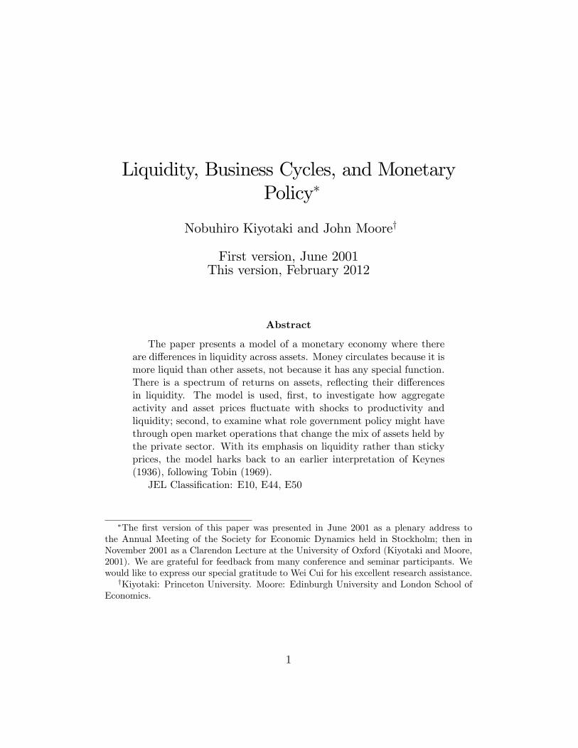
Figure 1. Impulse Responses of Basic Economy to Productivity Shock

0 2 0 4 0 6 0 8 0 1 0 00

0 .5

1

1 .5

%

a

0 2 0 4 0 6 0 8 0 1 0 00

0 .5

1

1 .5

2

%

I

0 2 0 4 0 6 0 8 0 1 0 00

0 .5

1

1 .5

%

C

0 2 0 4 0 6 0 8 0 1 0 00

0 .2

0 .4

0 .6

0 .8

%

K

0 2 0 4 0 6 0 8 0 1 0 00

0 .5

1

1 .5

%

Y

0 2 0 4 0 6 0 8 0 1 0 00

0 .5

1

1 .5

2

%

p

0 2 0 4 0 6 0 8 0 1 0 0­0 . 5

0

0 .5

1

%

q

Because capital stock is pre-determined, and the labor market clears, out-put increases by 1:43% (the same proportion as at). Then from the goodsmarket equilibrium condition (23) ; we observe the asset prices (pt; qt) haveto increase together with productivity in order to increase consumption andinvestment in line with the larger output. Although investment is moresensitive to the asset prices and thus increases proportionately more thanconsumption, the aggregate consumption of both entrepreneurs and workersincrease substantially (especially because workers�consumption is equal totheir wage income). This is di¤erent from the �rst best allocation underCondition 1, in which consumption would be much smoother than invest-

22

ment because, without the binding liquidity constraints, consumption woulddepend upon permanent rather than current income. The co-movement ofquantities and asset prices is also a unique features of the monetary equilib-rium with binding liquidity constraints. In contrast, in the �rst best Tobin�sq would always equal 1 and the value of money would always be zero.Now let us consider liquidity shocks. Figure 2 shows the impulse response

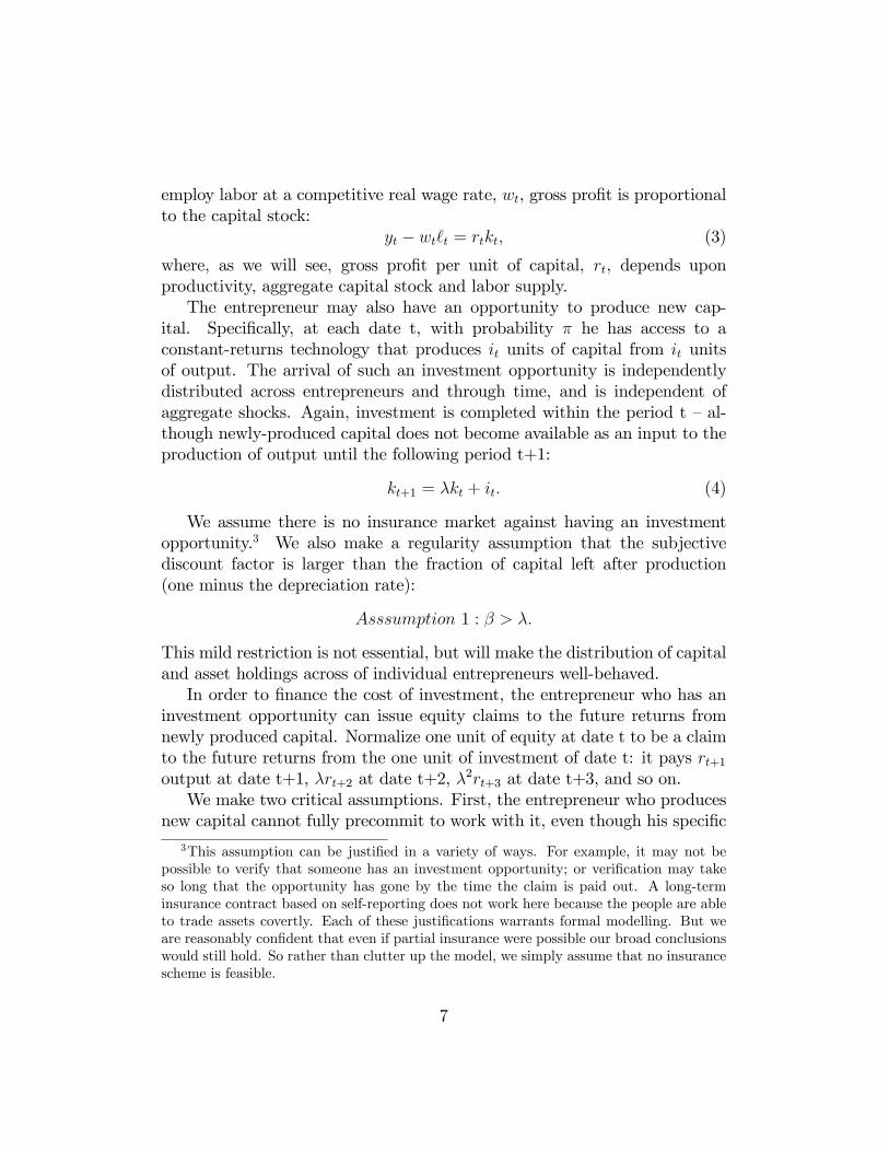
of quantities and asset prices against a 50% fall in the resaleability of theequity.

Figure 2. Impulse Responses of Basic Economy to Liquidity Shock

0 2 0 4 0 6 0 8 0 1 0 0­6 0

­4 0

­2 0

0

%

φ

0 2 0 4 0 6 0 8 0 1 0 0­8

­6

­4

­2

0

%

I

0 2 0 4 0 6 0 8 0 1 0 0­2

­1

0

1

2

3

%

C

0 2 0 4 0 6 0 8 0 1 0 0­2 . 5

­2

­1 . 5

­1

­0 . 5

0

%

K

0 2 0 4 0 6 0 8 0 1 0 0­1 . 5

­1

­0 . 5

0

%

Y

0 2 0 4 0 6 0 8 0 1 0 00

1 0

2 0

3 0

4 0%

p

0 2 0 4 0 6 0 8 0 1 0 00

5

1 0

1 5

%

q

When the resaleability of equity falls, and only slowly recovers, the in-vesting entrepreneurs are less able to �nance downpayment from selling theirequity holdings, and so investment decreases substantially. Capital stock and

23

output gradually decrease with persistently lower investment. Also the entre-preneurs without investment opportunities now �nd money more attractivethan equity as a means of saving (holding the rates of return unchanged),given that they can resale a smaller fraction of their equity holding whenfuture investment opportunities arise (see (24)). Thus, the value of moneyincreases compared to the equity price in order to restore asset market equi-librium. This can be thought of as a "�ight to liquidity": a �ight from equityto money.Notwithstanding this �ight from equity, the equity price tends to rise

with the fall in the liquidity. One way to understand why is to think ofthe gap between Tobin�s q and unity as a measure of the tightness of theliquidity constraint, which increases when the resaleability of equity falls.Another way is to observe that, because output is not a¤ected initially (givenfull employment), consumption must increase to maintain equilibrium in thegoods market; and consumption rises through the wealth e¤ect of a risein asset prices. This negative co-movement between investment, asset pricesand consumption is a shortcoming of our basic model �a shortcoming sharedby many macroeconomic model with �exible prices.10 We address this in thenext section.Note that, in contrast to our monetary equilibrium, the �rst best alloca-

tion would not react to the liquidity shock as the liquidity constraint wouldnot be binding.

4 Full Model with Storage and Government

We now present the full model. The negative co-movement in the basicmodel between investment, asset prices and consumption can be reversedby expanding the model to include an alternative liquid means of saving:storage. Speci�cally, suppose that an agent can store �tzt+1 units of goodsat date t to obtain zt+1 units of goods at date t+1, where zt+1 must benonnegative. Although the storage technology has constant returns to scaleat the individual level, it is decreasing returns to scale at the society level:�t is an increasing function of the aggregate quantity of storage Zt+1;

10Shi (2011) points out that in our basic model it is di¢ cult for a liquidity shock togenerate a positive co-movement in aggregate investment and the price of equity.

24

�t = � (Zt+1) =

�Zt+1�0

��; where �0; � > 0:

Storage represents all the various means of short-term saving besides money,such as consumer durables or net foreign asset (domestic residents can savein foreign assets but cannot borrow from foreigners).To complete the model, we also introduce government. Our goal here is

simply to explore the e¤ects on equilibrium of an exogenous government pol-icy rule. We make no attempt to explain government behavior. At the startof date t, suppose the government holds N g

t equity. Unlike entrepreneurs,the government cannot produce new capital. However, it can engage in openmarket operations, to buy (sell) equity by issuing (taking in) money �it hassole access to a costless money-printing technology. Any sale of equity issubject to the same constraint as (5).11 Finally, the government can pur-chase goods, or transfer goods to the workers (a negative would correspondto a lump-sum tax of the workers). Let Gt denote the total governmentpurchases. Assume that Gt does not a¤ect the entrepreneurs, which leavesintact our analysis of their behavior. We assume that N g

t and Gt are not solarge that the private economy switches regimes. That is, we are still in anequilibrium where the liquidity constraints bind for investing entrepreneursand money is valuable.If Mt is the stock of money privately held by entrepreneurs at the start

of date t, then the government�s �ow-of-funds constraint is given by

Gt + qt�N gt+1 � �N g

t

�= rtN

gt + pt(Mt+1 �Mt) = rtN

gt + (�t � 1)Lt; (31)

where Lt � ptMt are real balances, and �t �Mt+1

Mtis the money supply growth

rate. That is, cost of the government�s purchases of output and equity mustbe met by the dividends from its equity holding plus seigniorage revenues.Since government is a large agent, at least relative to each of the privateagents, open market operations will a¤ect the prices pt and qt.We will suppose that the government follows a rule for its open market

operations and �scal policy:

N gt+1

K= a

at � a

a+ �

�t � �

�(32)

11The government also is subject to the same resaleability constraint as the entrepreneur:Ngt+1 � (1� �t)�N

gt .

25

Gt = � [(rt + �qt)Ngt � (Lt � L)] ; (33)

where a; � and � are policy parameters, andK and L are capital stock andreal money balances in the non-stochastic steady state. The �rst equationis government�s feedback rule for its open market operations: it chooses thesize of open market operation (ratio of government equity holding to totalequity supply in the steady state) as a function of the proportional deviationsof productivity and liquidity from the steady state levels. This rule impliesthat the government�s equity holding is zero in the steady state. The secondequation is the �scal policy rule: the government adjusts its goods purchasesto be proportional to the deviation of its net asset holdings from steady stateat the beginning of each period. To limit the length of our discussion, wewill here report only on simulations with � = 0 so that Gt = 0; i.e. where allthe �scal adjustment is done through the money supply growth rate �t.The earlier analysis carries through, with obvious modi�cations. The

total supply of equity (which by construction is equal to the aggregate capitalstock) equals the sum of the government�s holding and the aggregate holdingof the entrepreneurs (denoted by Nt+1):

Kt+1 = N gt+1 +Nt+1: (34)

Workers consume all their disposable income, and, given the form of theirpreferences in (8), government policy does not a¤ect their labor supply.Equations (22) ; (23) and (24) are modi�ed to:

(1� �qt) It = ��� [(rt + ��tqt)Nt + Lt + Zt]� (1� �)(1� �t)�q

Rt Nt

(35)

atK�t + Zt = It + � (Zt+1)Zt+1 +Gt + (1� �) ��

[rt + (1� � + ��t)�qt + � (1� �t)�qRt ]Nt + Lt + Zt

(36)

(1� �)Et

�(rt+1 + �qt+1)=qt � Lt+1=(�tLt)

(rt+1 + qt+1�)N st+1 + Lt+1 + Zt+1

�= �Et

�Lt+1=(�tLt)� [rt+1 + �t+1�qt+1 + (1� �t+1)�q

Rt+1]=qt

[rt+1 + �t+1�qt+1 + (1� �t+1)�qRt+1]N

st+1 + Lt+1 + Zt+1

�(37)

(1� �)Et

�(rt+1 + �qt+1)=qt � (1=�(Zt+1))(rt+1 + qt+1�)N s

t+1 + Lt+1 + Zt+1

�

26

= �Et

�(1=�(Zt+1))� [rt+1 + �t+1�qt+1 + (1� �t+1)�q

Rt+1]=qt

[rt+1 + �t+1�qt+1 + (1� �t+1)�qRt+1]N

st+1 + Lt+1 + Zt+1

�; (38)

whereN st+1 = �It+�t��Nt+(1��)�Nt+�N

gt �N g

t+1. In the investment equa-tion, (35), entrepreneurs use their money, storage and the resaleable portionof their equity �net of their consumption �to �nance the downpayment. Inthe goods market equilibrium, (36) ; output (net of the worker�s consumption)plus storage return equals the sum of investment, new storage, governmentpurchases and entrepreneurs�consumption. (If storage were considered a netforeign asset, then the accumulation of net foreign assets, Zt+1�Zt; would bethe current account.) The portfolio equation (37) gives the trade-o¤ betweenholding equity and money. And the new portfolio equation (38) gives thetrade-o¤ between holding equity and storage.Restricting attention to a stable price process, competitive equilibrium is

de�ned recursively as functions�It; rt; Lt; qt; Zt+1; Kt+1; Nt+1; N

gt+1; Gt; �t+1

�of the aggregate state (Kt; Zt; N

gt ; at; �t) that satisfy (11),(25),(31) � (38)

together with the exogenous law of motion of (at; �t) :12

How does the presence of storage as alternative means of liquid savingstorage alter the impulse responses? Figure 3 compares the impulse re-sponses to a liquidity shock in the model without storage (taken from Figure2) and in the model with storage. We choose a storage technology that hasvery close to constant returns to scale (� = 0:0001), and is such that thesteady-state level of storage (�0 = 0:5) is modest compared to the steady-state capital stock (K = 9:49).In response to the fall in the resaleability of equity, storage increases

sharply, and investment falls more signi�cantly than the economy withoutstorage, leading to a more signi�cant fall in output.13 Importantly, consump-tion can now also fall along with investment, as output is soaked up by thesharp rise in storage.Also, because money and storage are very close substitutes �with a rate

12If there were a lump-sum transfer of money to the entrepreneurs (a helicopter drop),then aggregate quantities would not change in our economy given that prices and wages are�exible. The consumption and investment of individual entrepreneurs would be a¤ected,however, because there would be some redistribution.13In Bernanke and Gertler (1989), this is called "disintermediation": with greater fric-

tion in �nancial markets, more funds bypass those markets and are instead channelleddirectly into alternative investments �here, into storage �that may be productively infe-rior.

27

of return very close to one �the price of money is stable. Real balances hardlyincrease. As a consequence, the "�ight to liquidity" induces the equity priceto fall a little, at least initially.Taking these �ndings together, we see that the presence of an alternative

liquid means of saving has overcome the shortcomings of our basic model.Quantities (investment and consumption) and asset prices move together, asstorage serves as a bu¤er stock to absorb output and stabilize the value ofmoney.

Figure 3. Impulse Responses of Economy with Storage to Liquidity Shock

0 2 0 4 0 6 0 8 0 1 0 0­6 0

­4 0

­2 0

0

%

φ

0 2 0 4 0 6 0 8 0 1 0 0­3 0

­2 0

­1 0

0

1 0

%

I

0 2 0 4 0 6 0 8 0 1 0 0­4

­2

0

2

4

%

C

0 2 0 4 0 6 0 8 0 1 0 0­6

­4

­2

0

2

%

K

0 2 0 4 0 6 0 8 0 1 0 0­3

­2

­1

0

1

%

Y

0 2 0 4 0 6 0 8 0 1 0 00

2 0

4 0

6 0

8 0

1 0 0

%Z

0 2 0 4 0 6 0 8 0 1 0 00

1 0

2 0

3 0

4 0

%

L

0 2 0 4 0 6 0 8 0 1 0 00

5

1 0

1 5

%

q   w i t h o u t   s t o ra g e

0 2 0 4 0 6 0 8 0 1 0 0­0 .2

0

0 . 2

0 . 4

0 . 6

%

q   w i t h   s to ra g e

P u re   M o n e y

M o n e y   &   S t o ra g e

How might the government, through its central bank, conduct open mar-ket operations in response to the liquidity shock? A �rst-best allocation

28

would not be a¤ected by a liquidity shock. With this benchmark in mind, inour monetary economy the central bank should use open market operationsto o¤set the e¤ects of the liquidity shock, by setting the feedback rule coe¢ -cient � to be negative in (32). That is, the central bank should counteractthe negative shock by purchasing equity with money, in order to �at leastpartially �restore the liquidity of investing entrepreneurs. Figure 4 com-pares the impulse responses of the economy without this policy rule ( � = 0and � = 0, taken from Figure 3) and with the rule ( � = �0:1).

Figure 4. Impulse Responses of Full Model to Liquidity Shock

0 5 0 1 0 0­ 6 0

­ 4 0

­ 2 0

0

%

p h i

0 5 0 1 0 0­ 3 0

­ 2 0

­ 1 0

0

1 0

%

I

0 5 0 1 0 0­ 3

­ 2

­ 1

0

1

%

C

0 5 0 1 0 0­ 6

­ 4

­ 2

0

2

%

K

0 5 0 1 0 0­ 3

­ 2

­ 1

0

1

%

Y

0 5 0 1 0 00

5 0

1 0 0

%

Z

0 5 0 1 0 00

2 0

4 0

6 0

8 0

%

L

0 5 0 1 0 0­ 0 .5

0

0 .5

%

q

0 5 0 1 0 00

0 .2

0 .4

0 .6

0 .8

Diff

Ng/K

s t e a d y

0 5 0 1 0 0­ 5 0

0

5 0

1 0 0

%

µ

0 5 0 1 0 0­ 1

­ 0 .5

0

0 .5

1

Diff

G

N o  P o l i c y

W i th  P o l i c y

29

The central bank�s purchases of equity with money causes real balanceto increase sharply, notwithstanding the relatively stable price of money.Storage increases less than in the economy without the policy intervention.Investment falls initially by 30% �almost as much as in the case of no policy,because at the time of the shock the investing entrepreneurs�portfolios arepredetermined. However, in the following period, investing entrepreneurs(most of whom were savers in previous period) have a larger proportion ofliquid assets thanks to the policy intervention, and investment recovers to alevel of 10% below the steady state. Thus capital stock and output do notfall as much as in the economy without intervention.After the initial purchase of equity, government runs a surplus because

equity yields a higher return. It uses this surplus to reduce the moneysupply by setting �t < 1 (assuming no adjustment to government purchases).Because this de�ationary policy rewards money holders, the �ight to liquidityis more pronounced: the equity price falls as a result.In contrast, how might the central bank use open market operations in

response to a productivity shock? Once more taking the �rst-best allocationas a benchmark, the problem of our laissez-faire monetary economy is thatinvestment does not react enough to productivity shocks and consumption isnot smooth enough. Here the central bank should provide liquidity procycli-cally to accommodate productivity shocks, by setting the feedback coe¢ cientof a to be positive in (32). Figure 5 compares the impulse response func-tions of the laissez-faire monetary economy with an accommodating mone-tary policy ( a = 0:2 and � = 0). As productivity rises by 1:43%, the centralbank buys equity with money to provide an additional 4% liquidity (again,notwithstanding the relatively stable price of money). Entrepreneurs holdmore money and less illiquid equity, and thus investment more. Investmentincreases by 1:3% in the periods immediately following the shock, ratherthan increasing gradually as in the economy without the intervention. Butwhereas investment, and hence capital stock and output, all increase morebecause of the policy, storage and consumption increase less.

30

Figure 5, Impulse Responses of the Full Model to Productivity Shock

0 5 0 1 0 00

0 .5

1

1 .5

%

a

0 5 0 1 0 00

0 .5

1

1 .5

%

I

0 5 0 1 0 00

0 .5

1

1 .5

%

C

0 5 0 1 0 00

0 .2

0 .4

0 .6

0 .8

%

K

0 5 0 1 0 00

0 .5

1

1 .5

%

Y

0 5 0 1 0 00

2

4

6

%

Z

0 5 0 1 0 00

2

4

6

%

L

0 5 0 1 0 0­0 .2

0

0 .2

0 .4

0 .6

%

q

0 5 0 1 0 00

1

2

3x 1 0

­ 3

Diff

Ng/K

s t e a d y

0 5 0 1 0 0­2

0

2

4

%

µ

0 5 0 1 0 0­1

­0 .5

0

0 .5

1

Diff

G

N o  P o l i c y

W i th  P o l i c y

The e¢ cacy of these open market operations relies on the purchase of anasset �here, equity �which is only partially resaleable and hence earns a non-trivial liquidity premium. If the liquidity premium of short-term governmentbonds is very low (as in Japan since the late 1990s), then traditional openmarket operations will only serve to change the composition of broad moneyand will have limited e¤ects. The recent unorthodox policy of the FederalReserve Bank (and the Bank of England), such as the Term Security LendingFacility, is an attempt to increase liquidity by supplying treasury bills againstonly partially resaleable securities, such as mortgage backed securities.

31

5 Related Literature and Final Remarks

We hope to have succeeded in constructing a model of money and liquidityin the tradition of Keynes (1936) and Tobin (1969). The two key equationsof our model, (23) and (24) �which are generalized in (36) ; (37) and (38) �have the �avor of the Keynesian IS-LM system. We follow Tobin in placingemphasis on the spectrum of liquidity across di¤erent classes of asset. Also,Tobin�s q-theory �nds echo in our model through the central role played bythe equity price q: driving the feedback from asset markets to the rest of theeconomy. Our policy prescriptions �use open market operations to changethe liquidity mix of the private sector�s asset holdings � parallel those inMetzler (1951). Perhaps, with its focus on liquidity, our framework harksback to an earlier tradition of interpreting Keynes, and has less in commonwith the formal Keynesian literature, with its emphasis on sticky prices, thathas been dominant in the past few decades.This paper is part of the recent literature on macroeconomics with �nan-

cial frictions, that includes Bernanke and Gertler (1989), Kiyotaki and Moore(1997), Holmstrom and Tirole (1998).14 Naturally, the common thread ofthis literature has been some form of borrowing constraint, akin to our �-constraint. Our innovation here is to combine it with the �-constraint, theresaleability constraint. We have shown that the presence of these two con-straints opens up the possibility for �at money to circulate, to lubricate thetransfer of goods from savers to investors. There is a wedge between moneyand other assets, that arises out of the assumed di¤erence in their resaleabil-ity.Wedges between assets can be generated in other ways. In limited partic-

ipation models, agents may have di¤erent access to asset markets.15 Modelswith spatially separated markets �island models �assume that agents can-not visit all markets within the period, which limits trade across assets.Some models combine geographical separation with asynchronization, whereagents have access to asset markets at di¤erent times.16 If the assumptionof competitive markets is dropped, as in matching models, assets can ex-

14Surveys can be found in Bernanke, Gertler and Gilchrist (1999), Gertler and Kiyotaki(2010), Brunnermeier, Eisenbach and Sannikov (2011).15See, for example, Allen and Gale (1994, 2007).16See, for example, Townsend (1987), Townsend and Wallace (1987), Freeman (1996a,

1996b), and Green (1999).

32

hibit di¤erent degrees of resaleability.17 And there is a long tradition in thebanking and �nance literature that, implicitly or explicitly, has to do withthe limited resaleability of securities, dating back at least to Diamond andDybvig (1983).18

We should end by stressing that if, in particular, our model is to be usedfor proper policy analysis then considerably more research is still needed.While it might be argued that our �-� framework has the virtue of simplic-ity, as they stand the borrowing and resaleability constraints are too stylizedin nature, too reduced-form. The borrowing constraint can be rationalizedby invoking a moral hazard argument, viz., to produce future output fromnew capital requires the speci�c skill of the investing entrepreneur, and he canrenege on his promises. But the resaleability constraint requires more mod-elling, not least because we need to understand where the liquidity shocks,the shocks to �, come from.19 Can policies be devised that directly dampenthese shocks (or even raise the average value of �), rather than merely dealingwith their e¤ects?To analyze the e¤ects of open market operations over the business cycle,

we assumed that the government can commit to a policy. But can it? Thisquestion calls for further modelling too, because if the government couldcommit to, say, a de�ationary monetary policy that followed the Friedmanrule (set the real return on money to equal agents�subjective discount rate),then it would in e¤ect be using its taxation powers to substitute perfectpublic commitment for imperfect private commitment. In the long run, canthe government be trusted more than the private sector? And to what extentdo future tax liabilities crowd out a private agent�s ability to issue crediblepromises to others?20 These thorny issues warrant much careful thinking.

17Matching models that can be easily used for policy analysis include Shi (1997), Lagosand Wright (2005), and Nosal and Rocheteau (2011).18For attempts to incorporate banking into standard business cycle models, see, for

example, Wiiliamson (1987), Gertler and Kiyotaki (2010), Gertler and Karadi (2011).19Kiyotaki and Moore (2003) shows how the resaleability constraint can arise endoge-

nously due to adverse selection and how securitization may mitigate the adverse selection.Other macroeconomic models of adverse selection in asset markets inclde Eisfeldt (2004),

Moore (2010), Kurlat (2011).20A related question would be: If the government has a superior power to force private

agents to pay, why doesn�t it provide them with �nance directly?

33

6 References

Allen, Franklin, and Douglas Gale. 1994. "Limited Market Participationand Volatility of Asset Prices." American Economic Review 84(4): 933-955._______ and ______ 2007. Understanding Financial Crises. Ox-

ford: Oxford University Press.Bernanke, Ben, and Mark Gertler. 1989. "Agency Costs, Net Worth and

Business Fluctuations," American Economic Review 79(1): 14-31.Bernanke, Ben, Mark Gertler and Simon Gilchrist. 1999. "The Financial

Accelerator in a Quantitative Business Cycle Framework." In Handbook ofMacroeconomics, edited by John Taylor and Michael Woodford. Amsterdam,Netherlands: Elsevier.Brunnermeier, Markus, and Lasse Pedersen. 2009. "Market Liquidity

and Funding Liquidity." Review of Financial Studies 22(6): 2201-2238._______, Thomas Eisenbach and Yuliy Sannikov. 2011. "Macroeco-

nomics with Financial Frictions: A Survey." Manuscript for 2010 Economet-ric Society World Congress Monograph.Del Negro, Marco, Gauti Eggertsson, Andrea Ferrero and Nobuhiro Kiy-

otaki. 2011. "The Great Escape?: A Quantitative Evaluation of the Fed�sLiquidity Facilities." Sta¤ Reports 520. Federal Reserve Bank of New York.Diamond, Douglas, and Philip Dybvig. 1983. "Bank Runs, Deposit In-

surance, and Liquidity." Journal of Political Economy 91(3): 401-419.Eisfeldt, Andrea. 2004. "Endogenous Liquidity in Asset Markets." Jour-

nal of Finance 59(1): 1-30.Freeman, Scott. 1996a. "Clearinghouse Banks and Banknote Over-issue."

Journal of Monetary Economics 38(1): 101-115._______. 1996b. "Payment System, Liquidity, and Rediscounting."

American Economic Review 86(5): 1126-38.Gertler, Mark, and Peter Karadi. 2011. "A Model of Unconventional

Monetary Policy." Journal of Monetary Economics 58(1): 17-34.Gertler, Mark and Nobuhiro Kiyotaki. 2010. "Financial Intermediation

and Credit Policy in Business Cycle Analysis." InHandbook of Monetary Eco-nomics, edited by Benjamin Friedman and Michael Woodford. Amsterdam,Netherlands: Elsevier.Green, Edward. 1999. "Money and Debt in the Structure of Payments."

Federal Reserve Bank of Minneapolis, Quarterly Review 23: 13-29.Hart, Oliver, and John Moore. 1994. "A Theory of Debt Based on the

Inalienability of Human Capital." Quarterly Journal of Economics 109(4):

34

841-879.Holmstrom, Bengt. and Jean Tirole. 1998. "Private and Public Supply

of Liquidity." Journal of Political Economy 106(1): 1-40.Keynes, John Maynard. 1936. The General Theory of Employment, In-

terest, and Money. London: Macmillan.Kiyotaki, Nobuhiro, and John Moore. 1997. "Credit Cycles." Journal of

Political Economy 105(2): 211-248._______ and _______. 2001. "Liquidity, Business Cycles and

Monetary Policy: Manuscript of Clarendon Lecture 2." Mimeo. LondonSchool of Economics._______ and _______. 2002. "Evil is the Root of All Money."

American Economic Review: Papers and Proceedings 92(2): 62-66._______ and _______. 2003. "Inside Money and Liquidity."

Mimeo. London School of Economics._______ and _______. 2005a. "Liquidity and Asset Prices."

International Economic Review 46(2): 317-349._______ and _______. 2005b. "Financial Deepening." Journal

of European Economic Association: Papers and Proceedings 3(2-3): 701-713.Kurlat, Pablo. 2011. "Lemons Markets and the Transmission of Aggre-

gate Shocks." Mimeo. Stanford University.Lagos, Ricardo and Randalll Wright. 2005. "A Uni�ed Framework for

Monetary Theory and Policy Analysis." Journal of Political Economy 113(3):463-484.Metzler, Loyd A. 1951. "Wealth, Saving, and the Rate of Interest." Jour-

nal of Political Economy 59(2): 93-116.Moore, John. 2010. "Contagious Iliquidity." Technical Handout of Hur-

wicz Lecture at Latin American Society, Edinburgh University and LondonSchool of Economics.Nosal, Ed, and Guillaume Rocheteau. 2011. Money, Payments, and

Liquidity. Cambridge: MA. MIT Press.Shi, Shouyong. 1997. "A Divisible Search Model of Fiat Money," Econo-

metrica 65(1), 75-102._______. 2011. "Liquidity, Assets and Business Cycles." Mimeo,

University of Toronto.Tobin, James. 1969. "A General Equilibrium Approach to Monetary

Theory." Journal of Money, Credit, and Banking 1(1): 15-29.Townsend, Robert. 1987. "Asset Return Anomalies in a Monetary Econ-

omy." Journal of Economic Theory 41(5): 219-247.

35

_______ and Neil Wallace. 1987. "A Model of Circulating PrivateDebt: An Example with a Coordination Problem." In Contractural Arrange-ments for Intertemporal Trade, edited by Edward Prescott and Neil Wallace.Minneapolis, MN: University of Minnesota Press.Williamson, Stephen. 1987. "Financial Intermediation, Business Failures,

and Real Business Cycles." Journal of Political Economy 95(6): 1196-1216.Woodford, Michael. 2003. Interest and Prices. Princeton, NJ: Princeton

University Press.

36

7 Appendix

7.1 Proof of Claim 1

We construct a competitive equilibrium which satis�es Claim 1 under Con-dition 1. Suppose that inequalities (5) ; (6) and (10) are not binding. Thenfrom (7) ; we need qt = 1: (If qt were strictly larger than one, investing entre-preneurs would invest arbitrary large amount and (5) would be binding. If qtwere strictly smaller than one, investing entrepreneurs would not invest at all,which is not consistent with the equilibrium with positive gross investmentin the neighborhood of the steady state). Then the choice of entrepreneursand workers in the competitive equilibrium imply:

1 = Et

��ctct+1

(rt+1 + �)

�= Et

��c0tc0t+1

(rt+1 + �)

�; (A1)

rt = At

�`tKt

�1� wt = (1� )At

�Kt

`t

� = !(`t)

�

At(Kt) (`t)

1� = Ct + c0t +Kt+1 � �Kt;

where Kt is aggregate capital stock, `t is aggregate labor, and Ct and c0t areaggregate consumption of entrepreneurs and workers. Because these are theconditions for the �rst best allocation, the competitive equilibrium achievesthe �rst best allocation if (5) ; (6) and (10) are not binding. In this competi-tive equilibrium, we get pt = 0: (If pt were strictly positive with non-binding

(6) ; we would have 1 = Et

�� ctct+1

pt+1pt

�which would not be satis�ed in the

neighborhood of the steady state).Consider this competitive economy in which workers do not save so that

c0t = wt`t and aggregate investment is equal to aggregate saving of entrepre-neurs:

It = Kt+1 � �Kt = rtKt � Ct:

Using (7) with qt = 1 and pt = 0; the inequality (5) for the investing entre-preneur becomes

rtnt � ct = nt+1 � �nt � (1� �)it � �t�nt:

37

Aggregating this inequality for all the investing entrepreneurs, observing thearrival of the investment opportunity is iid. across entrepreneurs and overtime, we have

� (rtKt � Ct) = �It � (1� �)It � �t��Kt: (A2)

In the steady state, Condition 1 implies

�(1� �)K > (1� �)(1� �)K � ���K:

Then in the neighborhood of the steady state (in which I = (1 � �)K),inequality (A2) is satis�ed. Because pt = 0; (6) and the second inequality of(10) are not binding. Therefore under Condition 1, we can �nd a competitiveequilibrium in which the inequalities (5) ; (6) and (10) are not binding andc0t ' wt`t and n0t ' 0 in the neighborhood of the steady state. Claim 1(iv)follows from (A1). QED:

7.2 Derivation of Consumption and Portfolio Equa-tions

Let Vt(mt; nt) be the value function of the entrepreneur who holds money andequity (mt; nt) at the beginning of the period t before meeting an opportunityto invest with probability �. The Bellman equation can be written as

Vt(mt; nt) = � � Maxcit; it;m

it+1; n

it+1

st:(5)(6)(7)

�ln cit + �Et

�Vt(m

it+1; n

it+1)�

+(1� �) � Maxcst ;m

st+1; n

st+1

st:(5)(6)(7), it = 0

�ln cst + �Et

�Vt(m

st+1; n

st+1)�:

Solving the �ow-of-funds condition (14) and (15) for consumption cst and cit,

the Bellman equation is

Vt(mt; nt)

= � � Maxmit+1;n

it+1

�ln�[rt + �t�qt + (1� �t)�q

Rt ]nt + ptmt � qRt n

it+1 � ptm

it+1

�+�Et

�Vt(m

it+1; n

it+1)� �

+(1� �) � Maxmst+1;n

st+1

�ln�(rt + �qt)nt + ptmt � qtn

st+1 � ptm

st+1

�+�Et

�Vt(m

st+1; n

st+1)� �

:

38

Let Rmt+1 be the rate of return on money from date t to date t+1 andlet Rhh

0t+1 be the implied rate of returns on equity for the entrepreneur when

her type is h (h = i for investing and h = s for saving or non-investing) atdate t and h0 at date t+1, i.e.,

Rmt+1 =pt+1pt

;

Rsst+1 =rt+1 + �qt+1

qt; Rsit+1 =

rt+1 + ��t+1qt+1 + ��1� �t+1

�qRt+1

qt;

Rist+1 =rt+1 + �qt+1

qRt; Riit+1 =

rt+1 + ��t+1qt+1 + ��1� �t+1

�qRt+1

qRt:

Then the �rst order conditions are

1 = Et

���citciit+1

Riit+1 + (1� �)�citcist+1

Rist+1

�(A3)

1 > Et

���citciit+1

Rmt+1 + (1� �)�citcist+1

Rmt+1

�(A4)

1 = Et

���cstcsit+1

Rsit+1 + (1� �)�cstcsst+1

Rsst+1

�(A5)

1 = Et

���cstcsit+1

Rmt+1 + (1� �)�cstcsst+1

Rmt+1

�(A6)

where cht is date-t consumption of the entrepreneur of type h and chh0

t+1 isdate t+1 consumption of entrepreneur when her type is h at date t and h0

at date t+1.We guess that

cit = (1� �)�[rt + �t�qt + (1� �t)�q

Rt ]nt + ptmt

;

cst = (1� �) f(rt + �qt)nt + ptmtg ;nit+1 = �

�[rt + �t�qt + (1� �t)�q

Rt ]nt + ptmt

=qRt ;

mit+1 = 0;

nst+1 = �ft�[rt + �t�qt + (1� �t)�q

Rt ]nt + ptmt

=qt;

mst+1 = �(1� ft)

�[rt + �t�qt + (1� �t)�q

Rt ]nt + ptmt

=pt

39

ciit+1 = (1� �) [rt+1 + �t+1�qt+1 + (1� �t+1)�qRt ]n

it+1;

cist+1 = (1� �) (rt+1 + �qt+1)nit+1;

csit+1 = (1� �)�[rt+1 + �t+1�qt+1 + (1� �t+1)�q

Rt ]n

st+1 + pt+1m

st+1

;

csst+1 = (1� �)�(rt+1 + �qt+1)n

st+1 + pt+1m

st+1

:

where ft � qtnst+1=(ptm

st+1+qtn

st+1) 2 (0; 1) is the share of equity in portfolio

of the non-investing entrepreneur. Under this guess we learn

ciit+1cit

= �Riit+1; andcist+1cit

= �Rist+1;

and thus (A3) is always satis�ed. (A4) can be written as

1 > Et

��Rmt+1Riit+1

+ (1� �)Rmt+1Rist+1

�: (A7)

We also learn that

csit+1cst

= ��ftR

sit+1 + (1� ft)Rmt+1

�;

csst+1cst

= ��ftR

sst+1 + (1� ft)Rmt+1

�:

Thus (A5) and (A6) become

1 = Et

��

Rsit+1ftRsit+1 + (1� ft)Rmt+1

+ (1� �)Rsst+1

ftRsst+1 + (1� ft)Rmt+1

�;(A8)

1 = Et

��

Rmt+1ftRsit+1 + (1� ft)Rmt+1

+ (1� �)Rmt+1

ftRsst+1 + (1� ft)Rmt+1

�:(A9)

Then ft times the RHS of (A8) plus 1�ft times RHS of (A9) is always equalto 1, and one of (A8) and (A9) is not independent. Subtracting (A9) from(A8) side by side and arranging, we get

�Et

�Rmt+1 �Rsint+1

ftRsit+1 + (1� ft)Rmt+1

�= (1� �)

�Rsst+1 �Rmt+1

ftRsst+1 + (1� ft)Rmt+1

�: (A10)

This is equivalent to (24) in the text. Because qt > 1 > qRt in our equilibrium,we always have

Riit+1 > Rsit+1 and Rist+1 > Rsst+1:

40

In the neighborhood of the steady state equilibrium, we have

Riit+1 > Rsst+1 > Rmt+1:

Thus, comparing (A9) and (A7) ; we learn the inequality (A7) holds in theneighborhood of the steady state.

7.3 Proof of Claim 2

Let l be the ratio of real money balance to capital stock in the steady state.From (26; 27; 28) in the text, the steady state value of (r; q; l) solves

r = 1� �+ (1� �)�r + � (1� � + ��) q + �� (1� �) qR + l

�; (A11)

(1� �) (1� �q) = �[� (r + ��q)� �(1� �) (1� �) qR + �l]; (A12)

(1� �)

rq+ �� 1

(r + �q)�+ l= �

1� r+��q+�(1��)qRq

[r + ��q + �(1� �)qR]�+ l(A13)

where � = � (1� �) + (1� � + ��)� and qR = 1��q1�� as in the text.

From (A11) and (A12) ; we have�1 � (1� �)� ��

���rl

�=

�11

��+

�(1� �)(1� ��)

�hb� + ��� (1� �)

i !q

where � = 1��1�� , � = 1� �+ ��(1� �)� and b� = (1� �+ ���)�: Thus

��r = (1� � + ��)�+ (1� �)h���(1� �)� � b�i q (A14)

�l = (1� �)��h�� � ��(� + � � ��)� + b�i q: (A15)

Because �����(�+����)�+b� = ��(1��)(1��)�+���+� (1� �) > 0;we have

l > 0; i¤ q <(1� �)�

�� � ��(� + � � ��)� + b� � bq: (A16)

Then there is a monetary equilibrium with �nancing constraint only if bq > 1;or

(1� �) � + ��� < (1� �) (1� �) ;

41

i.e., Condition 1 in the text for the �rst best allocation is violated.(A13) can be written as

[r � (1� �)q]

�r � (1� �)q + q +

l

�

�= ��(q�1)

�r � (1� �)q + �

�q +

l

�

��(A17)

Together with (A14) and (A15) ; we have the condition for steady state q as

0 = (q)

� ���(q � 1)

0@ n(1� � + ��)�+ q

h(1� �)

����� � b��� ���

io h� (1� ��) + b�i

+��(1� �)h�+ q

����� � b��i

1A�n(1� � + ��)�+ q

h(1� �)

����� � b��� ���

io�0@ n

(1� � + ��)�+ qh(1� �)

����� � b��� ���

io h� (1� ��) + b�i

+�(1� �)h�+ q

����� � b��i

1A : (A18)

Then we learn

(1) = �(1��)��+ ���� � b��2 f(1� �) [�(1� ��)(1� �) + �] + � (1� �)g < 0:

Therefore the necessary and su¢ cient condition for the existence of mon-etary equilibrium with q 2 (1; bq) is

0 < (bq) : (A19)

Using (A16), (A19) becomes

0 < ��� (1� � � �) [�� � (1� �) + �� (1� �)]� [�� � (1� �)]��

= ��2��(1� �) (1� � � �)� [�� � (1� �)] (1� �+ ���) [�� �� (1� �) (1� �)] :

Multiplying both sides with 1� �; we get the condition

0 < ��2�(1� �)(1� �)[(1� �)(1� �)� (1� �)� � ���]

+[(� � �)(1� �)� (1� �)� � ���] [(1� �)(1� �) + ��(1� �)]

� [� (1� �) (1� �) + �(1� �) + ��(� + � � ��)] :

42

This is equivalent to Assumption 2 in the text. Therefore, under Assumption2, we have a competitive equilibrium in which �at money has a positive value(Claim 3(i) pt > 0) and qt > 1 (Claim 2(ii)). Claim 2(iii) directly followsfrom inequality (A4) or (A7) which we proved above given that qt > 1 in theneighborhood of the steady state. QED:

7.4 Proof of Claim 3

Claim 3(i):Under Assumption 2, we have (1� �) �+ ��� < (1� �)(1� �): Thus we

have

@ RHS of (A11)@q

= � (1� �)

�1� � + ��� �

1� �

1� ��

�> � (1� �)

��

(1� �)(1� �)> 0:

Given q > 1 and l � 0; we have from (A11)

r > 1� �+ (1� �)(r + �); or

r + � >1

�: QED:

Claim 3(iv):Suppose that 3(iv) is not true. From (A13) and (A11) respectively, we

haver

q� 1� �

andr

q� (1� �) � (1� �)

�r

q(1� �) + �(1� �) + �

�+1� �

ql:

Together these imply l < 0: This is contradiction. QED:

Claim 3(iii):From equation (A13), Claim 3(iv) implies r

q+ � > 1: QED:

Claim 3(ii):

43

Using qR < 1 < q in (A13) ; we have

(1� �) [r � (1� �)q] > ��q � r � ��q � � (1� �) qR

�; or

r � (1� �)q > ��� (q � 1) > 0:Hence, given l > 0; from (A17) it follows that

�(� + 1)

� + �< ��

�1� 1

q

�;

where � � rq+ �� 1 > 0 by Claim 3(iii). But from (A14) ;

1

q=

1

(1� � + ��)�

n��(� + 1� �)� (1� �)[��� (1� �) � � b�]o :

Substituting this to the above inequality, we get

�(� + 1)

��(� + �)+

���

(1� � + ��)�

< 1� 1

(1� � + ��)�

n��(1� �)� (1� �)[��� (1� �) � � b�]o :

The LHS of this inequality is increasing in �:Suppose Claim 3(ii) is not true, i.e., � � 1��

�: Then

1� �

���(1� � + ��)+

�(1� �)

(1� � + ��)�

< 1� 1

(1� � + ��)�

n��(1� �)� (1� �)[��� (1� �) � � b�]o :

Multiplying this inequality through by ���(1� � + ��)�; we have

(1� �) [1� �+ ��(1� �)�] + ���� (1� �)

< ���(1� � + ��) [1� �+ ��(1� �)�]� ���2�(1� �)

+�2�2�2�(1� �)(1� �)� ���(1� �)(1� �+ ���)�:

Cancel the two terms which do not have factor 1 � �; and divide by 1 � �;we get

(1� �+ ���) [1� ��� (1� �)] < 0; or

(1� �+ ���) [1� �� (1� �)] < 0:

This is contradiction. QED:

44