Inequality, Business Cycles, and Monetary-Fiscal

Policy∗

Anmol BhandariU of Minnesota

David EvansU of Oregon

Mikhail GolosovU of Chicago

Thomas J. SargentNYU

February 13, 2020

Abstract

We study optimal monetary and fiscal policy in a model with heterogeneous agents, in-complete markets, and nominal rigidities. We show that functional derivative techniquescan be applied to approximate equilibria in such economies quickly and efficiently. Oursolution method does not require approximating policy functions around some fixedpoint in the state-space and is not limited to first-order approximations. We apply ourmethod to study Ramsey policies in a textbook New Keynesian economy augmentedwith incomplete markets and heterogeneous agents. Responses differ qualitatively fromthose in a representative agent economy and are an order of magnitude larger. Con-ventional price stabilization motives are swamped by an across person insurance motivethat arises from heterogeneity and incomplete markets.

Key words: Sticky prices, heterogeneity, business cycles, monetary policy, fiscal policy

∗We thank Adrien Auclert, Benjamin Moll, and seminar participants at numerous seminars and confer-ences for helpful comments

1

1 Introduction

We compute optimal monetary and fiscal policies in a New Keynesian economy populated byagents who face aggregate and idiosyncratic risks. Agents differ in their wage, exposure toaggregate shocks, holdings of financial assets, and ability to trade assets. Incomplete finan-cial markets prevent agents from fully insuring risks. Firms are monopolistically competitive.Price adjustments are costly. We examine how a Ramsey planner’s choices of nominal in-terest rates, transfers, and flat-rate taxes on labor earnings, dividends, and interest incomerespond to aggregate shocks.

Analysis of Ramsey policies in settings like ours faces substantial computational chal-lenges. The aggregate state in a recursive formulation of the Ramsey problem includes thejoint distribution of individual asset holdings and auxiliary promise-keeping variables thathad been previously chosen by the planner. The law of motion for that high-dimensionalobject must be determined together with the optimal policies, and the distributions alongthe transition path differ substantially from the invariant distribution without aggregateshocks. These aspects render inapplicable common computational strategies that eitherapproximate policy functions after summarizing cross-sectional distributions with a smallnumber of moments or linearize around some time-invariant distribution.

To overcome this challenge, we develop a new computational approach that can beapplied to economies with substantial heterogeneity and does not require knowing their long-run properties in advance. Our approach builds on a perturbation theory that uses smallnoise expansions with respect to a one-dimensional parameterization of uncertainty. Eachperiod, along a sample path, we approximate policy functions by applying a perturbationalgorithm evaluated at the current cross-sectional distribution. We use approximate decisionrules for the current period to determine outcomes, including the cross-sectional distributionnext period. Then we obtain approximations of next period’s decision rules by perturbingaround that new distribution. In this way, we sequentially update points around whichpolicy functions are approximated along the equilibrium path.

Our perturbation approach requires repeatedly computing derivatives of policy func-tions with respect to all state variables. One state variable is a distribution over a multi-dimensional space of agents’ characteristics. Except for very simple models of heterogeneity,it is impractical to compute the derivative with respect to this distribution (i.e., the Frechetderivative). We prove that in a large class of heterogeneous agent competitive equilibriummodels this computationally-intensive step can be avoided and the problem of finding param-eters of the approximated policy functions can be written as a collection of low-dimensionalsystems of linear equations that are independent of each other. This property emerges be-cause in standard competitive environments, conditional on prices and aggregate quantities,

2

each agent’s optimal choices can be solved separately from those of others. These choicescan then be aggregated into feasibility constraints to solve a low-dimensional fixed pointproblem that determines prices and aggregate quantities. Because these systems of linearequations are independent across agents, they are easily parallelizable. This lets us handlethe ample heterogeneity present in our model. We go on to show that an analogous, com-putationally convenient, linear structure prevails for second- and higher-order expansions,making our approach applicable to many optimal policy problems in which aggregate riskshave important effects on equilibrium dynamics.

We apply our approach to a textbook New Keynesian sticky price model (see, e.g.,Galí (2015)) augmented with heterogeneous agents in the spirit of Bewley-Hugget-Aiyagari.Financial markets are incomplete and agents can trade only non-state-contingent nominaldebt. Agents’ wages are subject to idiosyncratic and aggregate shocks that we calibrate tomatch the U.S. business cycle and cross-sectional properties of labor earnings. We choose theinitial joint distribution of nominal claims, real claims, and wages to match cross-sectionalmoments in the Survey of Consumer Finances. We posit two types of aggregate shocks:a productivity shock and a shock to the elasticity of substitution between differentiatedintermediate goods that affects firms’ optimal markups. We study two types of Ramseypolicies. First, a “purely monetary policy” planner is required to keep all tax rates fixed,an assumption commonly used with New Keynesian models. In this case, the planner canadjust only nominal interest rates and a uniform lump-sum transfer. Second, a more powerful“monetary-fiscal” Ramsey planner can adjust tax rates on all sources of income in additionto interest rates and transfers.

In conventional representative agent New Keynesian models, the role for policy is inher-ited from a motive to stabilize inflation and the “output gap,” i.e., the difference betweenactual output and the first-best level of output. In our setting, households differ in theirshares of labor, dividend, and bond income and, therefore, in their exposures to aggregateshocks. Without a complete set of Arrow securities agents cannot hedge risk, so aggregateshocks affect agents differentially. While the planner uses the expected path of taxes andtransfers to redistribute and provide insurance with respect to idiosyncratic risk, how opti-mal policy deviates from this path is governed by a necessity to provide insurance againstaggregate shocks. In the calibrated economy, the welfare gains from providing insurance aremuch larger than the benefits of price stability, and the optimal monetary responses in ourheterogeneous agent economy are both quantitatively larger and qualitatively different fromthose in its representative agent counterpart.

To understand how insurance concerns shape policy responses, consider the optimal mon-etary response to a one-time positive markup shock. One effect of this shock, traditionallyemphasized by the New Keynesian literature, is that firms want to increase their prices.

3

To maintain price stability, the planner can increase nominal interest rates which lowersaggregate demand and, hence, firm’s marginal costs. This response forms the basis for theclassical prescription of “leaning against the wind” and raising interest rates when firms’desired markups are high (Galí (2015)). The markup shock also changes the relative sharesof payments that go to labor and equity. Such movements in factor shares have no welfareconsequences when firm owners and wage earners are the same people, but has importantinsurance implications when agents are heterogeneous. When agents cannot trade Arrowsecurities, the planner can use monetary and fiscal policy to substitute for missing insurancemarkets. Since a positive markup shock creates an unexpected drop in wage income (and awindfall in profits), the planner provides insurance by lowering nominal rates to boost wages.A negative markup shock reverses insurance needs, and therefore the optimal response is amirror image of the response to a positive markup shock.

Quantitatively, the strength of the insurance motive depends on the correlation of laborand capital income, with smaller correlations calling for higher insurance needs. In thedata the distribution of stock ownership is much more skewed than the distribution of laborearnings, which implies large welfare gains from insurance. As a result, in our calibratedeconomy optimal monetary responses to markup shocks are an order of magnitude largerand go in the opposite direction from those in the representative agent economy.

The insurance motive also shapes Ramsey responses to TFP shocks. While TFP shocksaffect profits and wages in the same way, the effects of TFP shocks are not shared equallyacross borrowers and lenders. When borrowing is not state contingent, a TFP shock changestotal output while keeping nominal obligations unchanged. A negative TFP shock hurtsborrowers while a positive TFP shock hurts lenders. The planner can provide insuranceand improve welfare by lowering (raising) the real return on debt in response to a negative(positive) TFP shock. Such a policy contrasts with the standard New Keynesian prescriptionof adjusting the nominal rate one-for-one with the “natural” rate of interest in the flexibleprice economy. Since there is a large dispersion of nominal claims in the data, the insurancemotive is strong in the calibrated economy. We find that the optimal response to a mean-reverting negative TFP shock is to lower nominal as well as real rates of interest despite thefact that the “natural” rate increases.

We also show that, in providing insurance, there exists a trade-off between the on-impactmagnitude and the overall duration of the monetary response to a shock. The New KeynesianPhillips curve implies that current inflation is equal to the present value of all future wages.When all agents can freely borrow and lend, their utilities depend only on the present valueof their income. Therefore, an efficient monetary response minimizes costs of future inflationby front-loading all insurance: monetary policy responds aggressively to the shock at thetime of the impact but this response is short lived. When some agents face trading frictions,

4

the planner also needs to smooth the insurance provision over time. Monetary responsesbecome smaller in magnitude but longer lasting.

The role of monetary policy is diminished when the planner can also use fiscal instrumentsto respond to aggregate shocks. In the representative agent economy, the planner can fullyoffset the effect of markup shocks by changing labor taxes, financed through lump sumtransfers, making monetary policy redundant. This response is no longer optimal whenagents are heterogeneous, because it increases the volatility of the after-tax income of lowwage earners relative to high wage earners. We show that it is more efficient to use dividendor corporate profit taxes in response to markup shocks when agents are heterogeneous. Forsimilar reasons, adjusting taxes on interest income is an efficient fiscal response to TFPshocks.

1.1 Related literature

Our paper contributes to two literatures, one that approximates equilibria of incompletemarkets economies with heterogeneous agents, and another that computes Ramsey plans forfiscal and monetary policies.

We use small noise expansions around transition paths like those deployed by Fleming(1971), Fleming and Souganidis (1986), and Anderson et al. (2012). Those authors applythis approach only to problems with low-dimensional states. The state in our model includesa joint distribution over a multi-dimensional domain, a feature that gives us a much largerstate space and makes direct application of the approaches taken in those earlier papers com-putationally infeasible. To meet these challenges, we introduce functional derivatives tech-niques1 to cope with the most computationally intensive step and reformulate the problemof computing approximate policy functions as a manageable collection of small-dimensionallinear equations. We also show how our techniques can be used to construct second- andhigher-order approximations via a convenient set of recursions.

There are trade-offs in applying our method as compared to other popular approachessuch as Krusell and Smith (1998) or Reiter (2009). Relative to Krusell and Smith (1998),our method is not restricted to problems in which a small number of moments are enoughto summarize how policy functions depend on the distribution of agents’ characteristics. Ina Reiter-type approach, policy functions are accurate with respect to idiosyncratic shocks,but are approximated only to the first order with respect to aggregate shocks around theinvariant distribution of the no-aggregate-shock economy. In comparison, our method isnot restricted to linear approximations, and we repeatedly update the coefficients of the

1Childers (2018) combines related functional derivative techniques with a Reiter (2009) method, butunlike our approach, his still requires that distributions remain close to the invariant distribution of ano-aggregate-shock economy. We build on and extend Evans (2015).

5

approximation as the state of the economy moves along the equilibrium path. Our methodis particularly well suited when the economy features non-trivial or even non-stationarytransition dynamics; when impulse responses depend on past realizations of shocks; or whenhigher-order moments of aggregate variables, such as risk premium, play an important role.It comes at a cost that we approximate less well the dependence of policy functions onidiosyncratic shocks.

We study the numerical accuracy of our method by computing the competitive equi-librium given fixed government policies for a special case of our model, which correspondsto the economy studied by Acharya and Dogra (2018). The advantage of this economy isthat it is possible to compute the equilibrium analytically without requiring approximations.This allows us to compare both our approximation and Reiter’s to the true solution. UnderAcharya and Dogra (2018) calibration, the maximum numerical errors in our approximatedpolicy functions are less than 0.05%. Moreover, the approximation errors in policy functionsfor aggregate variables are two orders of magnitude smaller than the ones obtained underReiter’s method. While our method is less accurate with respect to idiosyncratic shocks,those errors wash out in the aggregate; on the other hand, the second-order errors fromthe aggregate shocks under Reiter’s method do not. Moreover, we also show how theseerrors from aggregate shocks compound over time under Reiter’s approach, affecting thedistribution in the long run. Finally, we also illustrate how the drift of the distribution ofassets away from the point of approximation leads to errors in impulse responses under theReiter-based method which do not exist in our method.

A substantial literature on optimal monetary and fiscal policies in the Ramsey traditionhas mostly studied economies with limited or no sources of heterogeneity. For a textbooklevel treatment of optimal monetary policies in representative agent New Keynesian modelssee Galí (2015) and Woodford (2003).2 Papers such as Bilbiie and Ragot (2017), Challe(2017), Bilbiie (2019), and Debortoli and Gali (2017) study optimal monetary policy ineconomies with very limited heterogeneity and in which a cross-sectional distribution dis-appears from the formulation of the Ramsey problem and the analysis can be done usingtraditional techniques. Like us, those papers emphasize that uninsurable aggregate shockscreate reasons for the planner to compromise price stability. Recent papers by Legrandand Ragot (2017) and Nuno and Thomas (2016) develop alternative methods different fromours to approximate Ramsey allocations in incomplete market economies with heterogene-ity. Legrand and Ragot (2017) apply their method to a neoclassical economy and Nuno andThomas (2016) study transition dynamics of a Ramsey allocation in an small open economysetting.

2There are several papers that study optimal monetary and fiscal policies in calibrated representativeagent settings. For instance, see Chari and Kehoe (1999) for a neoclassical setup, Schmitt-Grohe and Uribe(2004a) and Siu (2004) for optimal responses to government spending shocks in setups with nominal rigidities.

6

2 Environment

Our economy is inhabited by a continuum of infinitely lived households. Individual i’spreferences over final consumption good ci,tt and hours ni,tt are ordered by

E0

∞∑t=0

βtu (ci,t, ni,t) , (1)

where Et is a mathematical expectation operator conditioned on time t information, β ∈(0, 1) is a time discount factor, and u is an infinitely differentiable utility function thatis concave in c and −n and satisfies the Inada conditions. We denote its derivatives byuc,i,t ≡ uc (ci,t, ni,t), un,i,t ≡ un (ci,t, ni,t), and so on. A random variable with subscript t ismeasurable with time t information.

Agent i who works ni,t hours supplies εi,tni,t units of effective labor, where εi,t is anexogenous productivity process. Effective labor receives nominal wage PtWt, where Pt isthe nominal price of the final consumption good at time t. Agents trade a one-period risk-free nominal bond with price Qt in units of the final consumption good. We use Ptbi,t todenote face value of nominal bonds owned by agent i and Ptdi,t to denote nominal dividendsfrom intermediate goods producers. Let Πt = Pt

Pt−1− 1 denote the net inflation rate. The

budget constraint of household i at date t in units of final goods is

ci,t +Qtbi,t = (1−Υnt )Wtεi,tni,t + Tt +

(1−Υd

t

)di,t +

(1−Υb

t

) bi,t−1

1 + Πt. (2)

All agents receive the same uniform lump-sum transfer Tt, and face a linear tax Υnt on their

labor earnings, a tax Υdt on their dividends, and a tax Υb

t on their bond income.3 Thegovernment’s budget constraint at time t is

G+ Tt +Bt−1

1 + Πt=

∫i

[ΥntWtεi,tni,t + Υd

t di,t +Υbtbi,t−1

1 + Πt

]di+QtBt,

where G is a time-invariant level of non-transfer government expenditures.A final good Yt is produced by competitive firms that use a continuum of intermediate

goods yt(j)j∈[0,1] in a production function

Yt =

[∫ 1

0yt(j)

Φt−1Φt dj

] ΦtΦt−1

,

3Although Υbt multiplies bi,t−1, we refer to it as a tax on the bond income because it is equivalent to a

tax on the return on a one-period bond. To see this, rewrite the budget constraint using the market valueof nominal debt bi,t = Qtbi,t, and notice that the term

(1−Υb

t

) bi,t−1

1+Πt=(1−Υb

t

)(Rt−1,t) bi,t−1, where

Rt−1,t =(

1Qt−1

)(1

1+Πt

)is the real return from holding a nominal bond from t− 1 to t.

7

where the elasticity of substitution Φt is stochastic. Final good producers take the finalgood price Pt and the intermediate goods prices pt(j)j as given and solve

maxyt(j)j∈[0,1]

Pt

[∫ 1

0yt(j)

Φt−1Φt dj

] ΦtΦt−1

−∫ 1

0pt(j)yt(j)dj. (3)

Outcomes of optimization problem (3) are a demand function for intermediate goods

yt(j) =

(pt(j)

Pt

)−Φt

Yt, (4)

and a final goods price satisfying

Pt =

(∫ 1

0pt(j)

1−Φt

) 11−Φt

.

Intermediate goods yt(j) are produced by monopolists with production functions

yt(j) =[nDt (j)

]α[ht (j)]1−α , (5)

where nDt (j) is effective labor hired by firm j and ht (j) is an intermediate input measuredin units of the final good. Intermediate goods monopolists face downward sloping demand

curves(pt(j)Pt

)−ΦtYt and choose prices pt(j) while bearing quadratic Rotemberg (1982) price

adjustment costs ψ2

(pt(j)pt−1(j) − 1

)2measured in units of the final consumption good. Inter-

mediate goods producing firm j chooses prices pt(j)t and factor inputsht(j), n

Dt (j)

t

that solve

maxpt(j),nD

t (j),ht(j)t

E0

∑t

St(1−Υdt )

pt(j)

Ptyt(j)−Wtn

Dt (j)− ht (j)− ψ

2

(pt(j)

pt−1(j)− 1

)2

(6)

subject to (4) and (5), where Wt is the real wage per unit of effective labor and St is thestochastic discount factor (SDF) defined recursively via

St = St−1Qt−1(1 + Πt)/(

1−Υbt

), (7)

with S−1 = 1.4 In a symmetric equilibrium, pt(j) = Pt, yt(j) = Yt, ht (j) = Ht, nDt (j) = Nt

4In economies with heterogeneous agents and incomplete markets, a stand must be taken on how firmsare valued. To explain our numerical methods most transparently we chose a simple specification of theSDF that discounts future profits at the after-tax real risk-free rate. Our quantitative results are virtuallyidentical when we use other popular choices of SDFs.

8

for all j. Market clearing conditions in labor, goods, and bond markets are

Ct =

∫ci,tdi, Nt =

∫εi,tni,tdi, Dt = Yt −Ht −WtNt −

ψ

2Π2t , (8)

Yt = Nαt H

1−αt , Πt = Pt/Pt−1 − 1 (9)

Ct + G = Yt −Ht −ψ

2Π2t , (10)∫

ibi,tdi = Bt. (11)

There are aggregate and idiosyncratic shocks. Aggregate shocks are a “markup” shockΦt and an aggregate productivity Θt that follow AR(1) processes

ln Φt =ρΦ ln Φt−1 + (1− ρΦ) ln Φ + EΦ,t,

ln Θt =ρΘ ln Θt−1 + (1− ρΘ) ln Θ + EΘ,t,

where EΦ,t and EΘ,t are mean-zero random variables that are i.i.d. over time.Individual productivity εi,t follows a stochastic process described by

ln εi,t = ln Θt + ln θi,t + εε,i,t, (12)

ln θi,t = ρθ ln θi,t−1 + εθ,i,t, (13)

where innovations εε,i,t and εθ,i,t are mean-zero, uncorrelated with each other, and i.i.d. overtime.

We set the initial price level P−1 = 1. Agent i in period 0 is characterized by a triple(θi,−1, bi,−1, si), where θi,−1 is agent i’s persistent component of productivity, bi,−1 denotesthe bonds that agent i initially owns, and si denotes agent i’s initial ownership of equity. Inwhat will serve as our baseline specification, we assume that agent i’s dividends in period tare di,t = siDt. This imposes that agents do not trade equity and that si is a permanentcharacteristic. We denote the collection θi,−1, bi,−1, sii as an initial condition.

Definition 1. Given an initial condition and a monetary-fiscal policy Qt,Υt, Ttt, a com-petitive equilibrium is a sequence

ci,t, ni,t, bi,ti , Ct, Nt, Bt,Wt, Pt, Yt, Ht, Dt,Πt, St

tsuch

that: (i) ci,t, ni,t, bi,ti,t maximize (1) subject to (2) and natural debt limits;5 (ii) final goodsfirms choose yt(j)j to maximize (3); (iii) intermediate goods producers’ prices and factor

5Natural debt limits are enforced by requiring a transversality condition

lims→∞

Et

(s∏

k=1

Qt+k

)bi,t+s = 0.

9

inputs solve (6) and satisfy pt(j) = Pt, yt(j) = Yt, ht (j) = Ht, nDt (j) = Nt for all j; and

(iv) market clearing conditions (8)-(11) are satisfied.

A Ramsey planner orders allocations by

E0

∫ ∞∑t=0

βtϑiu (ci,t, ni,t) di, (14)

where ϑi ≥ 0 is a Pareto weight attached to agent i with∫ϑidi = 1.

Definition 2. Given an initial condition and a time-invariant tax policy satisfying Υt = Υ

for some Υ, an optimal monetary policy is a sequence Qt, Tt t that implements a com-petitive equilibrium allocation that maximizes (14). Given an initial condition, an optimalmonetary-fiscal policy is a sequence Qt,Υt, Ttt that implements a competitive equilibriumallocation that maximizes (14). A maximizing monetary or monetary-fiscal policy is calleda Ramsey plan; an associated allocation is called a Ramsey allocation.

We characterize competitive equilibria by the feasibility constraints (7), (8), (9), and(10); the consumer and firm optimality conditions

(1−Υnt )Wtεi,tuc,i,t = −un,i,t, (15)

Qtuc,i,t = βEtuc,i,t+1

(1−Υb

t+1

)/ (1 + Πt+1)−1 , (16)

1

ψYt

[1− Φt

(1− 1

1− α

(1− αα

Wt

)α)]−Πt(1+Πt)+Et

St+1

St

(1−Υd

t+1

1−Υdt

)Πt+1(1+Πt+1)2 = 0,

(17)

1− αα

Wt =Ht

Nt, (18)

and agents’ budget constraints that, by using equation (15) to eliminate Wt and Υnt+1, we

can represent as

ci,t−Tt− (1−Υdt )siDt−

(1−Υbt)bi,t−1

1 + Πt=

(un,i,tuc,i,t

)ni,t+Et

(uc,i,t+1

uc,i,t

)(1−Υb

t+1)bi,t

1 + Πt+1. (19)

We can construct an optimal monetary-fiscal policy and an associated competitive equi-librium to maximize the welfare criterion (14) subject to these constraints. Choice of anoptimal monetary policy is subject to the additional constraints Υt = Υ for all t ≥ 0.

10

2.1 Discussion of the environment

We want to understand how optimal policies respond to aggregate shocks and what economicforces motivate those responses. To help us do so, we use two baselines that differ in whetheror not the Ramsey can adjust tax rates. In what we call our optimal monetary-fiscal policybaseline, in response to aggregate shocks, the Ramsey planner can freely adjust both thenominal interest rate and all tax rates. In what we call our optimal monetary policy baseline,the Ramsey planner can adjust only the nominal interest rate. Our use of a pure monetarypolicy baseline follows a New Keynesian tradition that, in our notation, assumes time-invariant tax rates Υt = Υ and that only the nominal interest rateQ−1

t can respond to shockswith Tt adjusting to satisfy the government’s budget constraint. A popular justification forthis restriction is that central banks adjust interest rates fast enough to react to shocks atbusiness cycle frequencies, while institutional constraints prevent adjusting tax rates quicklyand often. In principle, one can study optimal monetary policy for any arbitrary Υ, but inthe spirit of the New Keynesian literature, in our section 4 quantitative application, we focuson the level of Υ that maximizes welfare (14) under the optimal monetary policy associatedwith that Υ.

Our environment extends a textbook New Keynesian model along the lines of Galí (2015,ch. 3) to allow for incomplete markets and heterogeneous agents in the tradition of Bewley-Hugget-Aiyagari. An advantage of using this canonical New Keynesian setup is that norma-tive prescriptions for the representative agent economy are widely understood. That allowsus to isolate modifications of those prescriptions that heterogeneity and incomplete mar-kets bring. In our baseline environment, we model heterogeneity using a standard processfor wage dynamics from the macro labor literature, for instance as in Low et al. (2010) orStoresletten et al. (2001). In section 6.3, we enrich the baseline process for wage dynamics toallow for diverse responses of labor earnings to recessions that are documented by Guvenenet al. (2014).

In our two baseline models, we assume that all agents can freely trade bonds subjectto natural debt limits. This means Ricardian equivalence holds and timing of transfersis undetermined.6 This is a natural baseline as economies with ad hoc debt limits oftenprescribe ad hoc non-stationary optimal fiscal policy by front-loading transfers to undo thoseconstraints.7 We relax this assumption in section 6.1 when we prevent a subset of agents

6In the general formulation of the Ramsey problem, we do not restrict lump-sum transfers Tt to bepositive. However, in our section 4 quantitative application, transfer are always positive since householdsare unequal and planner cares about redistribution.

7In Bhandari et al. (2017) we provide a comprehensive treatment of a Ramsey problem with ad hoc debtlimits. In the economy with ad hoc debt limits the planner can simply choose the timing of transfers to undosuch ad hoc debt limits. If the planner enforces debt and tax liabilities equally then welfare in the economieswith ad hoc and natural debt limits coincides. Welfare can sometimes be improved in the economy withad hoc debt limits if the planner commits not to enforce private debt contracts (see also Yared (2013) for a

11

from trading the risk-free bond or other assets.In our baseline models, we also assume that agents can trade debt but not equity. This

specification yields several insightful special cases that we find useful for explaining ournumerical methods and economic forces in the model. We relax the nontradability of claimsto dividends in section 6.2 when we introduce mutual funds that hold corporate equity andgovernment debt and that issue mutual fund shares to households who trade them in acompetitive market.

3 Approximation method

We approximate Ramsey plans for heterogeneous agents (HA) economies that by their verynature have state vectors that include joint distributions of agents’ characteristics. Forreasons anticipated in section 1.1, this feature impelled us to depart from approximationmethods used by earlier authors such as the projection method of Krusell and Smith (1998)and the perturbation-around-a-no-aggregate-shock-economy method used by Reiter (2009).

The Krusell-Smith approach works well when the dimension of the state is low (e.g.,a univariate distribution), and policy functions admit approximate aggregation. Even inthe simplest versions of our problem, the state variable is a multivariate distribution, andapplication of a Krusell-Smith strategy would require tracking higher-order moments and becomputationally very expensive. The Reiter approach was designed for situations in whicha no-aggregate-shock invariant distribution is easy to compute and when it is known thatthe state in an economy with aggregate shocks always remains close to the no-aggregateshock invariant distribution. This condition might prevail in competitive equilibria underarbitrarily fixed government policies, but it is not in our setting.8

In this section, we propose an alternative method of solving HA economies. The keystep in our analysis is to demonstrate how functional derivative techniques can be used tocharacterize the dependence of policy functions on a high-dimensional state that changesover time in response to aggregate shocks. These computational techniques are fast andwork at any order of approximation.9

related result).8The long-run behavior of the state variables even in the simplest Ramsey problems can differ dramatically

with and without aggregate shocks in otherwise identical economies. One can easily see this from the classictax-smoothing paper by Barro (1979). In his economy, government debt is the only state variable. It staysalways at its initial level in the economy without aggregate shocks and follows a random walk with aggregateshocks. This law of motion has very different implications for the long-run distribution of debt in these twocases. Similarly, Aiyagari et al. (2002), Farhi (2010), Bhandari et al. (2017) all study Ramsey policies andfind that the invariant distribution of the state variables, while being well defined in all cases they consider,is discontinuous with respect to the size of aggregate shocks around the no-aggregate-shock level.

9We extensively discuss the comparison of our techniques to alternatives in section 3.3, but a readermay find the following informal summary helpful at this point. Perturbation methods of Reiter (2009)and Kaplan et al. (2018) are exact with respect to the dependence of policy functions on idiosyncratic

12

Section 3.1 considers a special case of our environment by setting parameters so that thesole state variable in a recursive formulation of a continuation Ramsey problem is a jointdistribution of agents’ characteristics. This case allows us to describe our techniques in afairly transparent way. Section 3.2 then tells how to extend our approach to the generalenvironment. Section 3.3 discusses numerical accuracy and computational speed and makescomparisons with earlier methods for approximating equilibria of HA economies.

3.1 An informative special case

To obtain a case that explains our methods in a transparent manner, we focus on optimalmonetary-fiscal policy for a utilitairan planner and impose: (i) equity holdings si are uniformacross households; (ii) α = 1 so that no intermediate goods are used as inputs; (iii) allshocks are i.i.d. These three restrictions are designed to make the state space as small aspossible while keeping it large enough to preserve the essence of our technique. The first twoassumptions imply that the Phillips curve constraint (17) is slack in all periods and so can beomitted from the Ramsey planner’s maximization problem. The third assumption impliesthat past shocks do not appear as arguments in optimal policy functions. Therefore, thestate becomes just a distribution of individual endogenous characteristics that summarizeindividual optimality conditions (15), (16), and (19).

Our focus in this section will be on characterizing how policy functions depend on thatdistributional state. There are several mathematically equivalent ways to choose the statespace to formulate our problem recursively. Our approach works best when a state spacesatisfies an independence property that we formally define below. In the simple economythat we consider in this section, most commonly used choices for state variables satisfy thisproperty. For clarity of exposition and consistency, we adopt a recursive formulation of aRamsey problem that preserves the independence property in more general settings.

Let Mt ≡∫uc,i,tdi be the average marginal utility of consumption at time t, and let

mi,t ≡ uc,i,t/Mt be scaled marginal utility of consumption of agent i at time t. We caninterpret mi,t as (an inverse of) a Pareto-Negishi weight that the planner attaches to agent

shocks but only first-order approximate with respect to aggregate shocks, all around a fixed distributionΩ. The approximation errors in this approach are thus on the order of O

(σ2agg, ‖Ω− Ω‖2

), where σagg is a

measure of the size of aggregate shocks. Childers (2018) provides a formal treatment. Our approach usesexpansions with respect to both aggregate and idiosyncratic shocks around the time t distribution Ωt inthat period, and can be done to an arbitrary order of approximation. Approximation errors are of the orderO(σn+1agg , σ

n+1idiosync

)for arbitrary n. The two approaches are therefore complementary and have advantages

and disadvantages that depend on specific applications.

13

i in time t. Replace (16) with

QtMtmi,t = βEtuc,i,t+1

(1−Υb

t+1

)/ (1 + Πt+1)−1 , mi,t = uc,i,t+1/Mt, Mt =

∫uc,i,t+1di.

(20)Let βtµi,t be a Lagrange multiplier on constraint (19) for agent i. Following Marcet andMarimon (2019), the monetary-fiscal Ramsey planner’s Lagrangian is

inf sup E0

∞∑t=0

βt∫ [

ϑiu (ci,t, ni,t) +(uc,i,tci,t + un,i,tni,t − uc,i,t(Tt +

(1−Υd

t

)Dt))µi,t

+(

1−Υbt

) bi,t−1

1 + Πtuc,i,t (µi,t−1 − µi,t)

]di (21)

subject to µi,−1 = 0 and where the infimum is taken with respect to µi,t, and the supremumis taken with respect to the sequence

ci,t, ni,t, bi,t,mi,t, Ct, Nt, Dt, Tt,Mt, Qt,Πt,Υti,t

subject to constraints (8)-(10), (15), and (20).It can be verified that a time t > 0 continuation Ramsey problem associated with

problem (21) is recursive in an aggregate state that consists of a bivariate distributionover zi,t−1 ≡ (mi,t−1, µi,t−1). We denote this distribution by Ω, and use z to denote atypical value in the support of Ω. We solve (21) in two steps. First, we solve continuationRamsey planners’ problems for t > 0. Second, we solve a time t = 0 Ramsey problem toobtain the t = 0 allocation ci,0, ni,0t as well as Ω0 as functions of an initial conditionθi,−1, si,−1, bi,−1i.

We use tildes to denote policy functions for the t > 0 continuation Ramsey plan. Theaggregate policy functions determine the time t values of all upper-case choice variablesin problem (21). We denote the nX dimensional vector of these functions by X (Ω,E),where E are aggregate shocks. Individual policy functions determine all lower-case time tchoice variables for the planner in problem (21). We denote individual policy functions byx (z,Ω, ε,E), where ε are idiosyncratic shocks. Policy functions for individual states z arecomponents of x. We define p to be a selection matrix that returns z from x, i.e., z = px.The law of motion for the aggregate state variable is denoted by Ω (Ω,E).

Consider the full set of t ≥ 1 first-order optimality conditions for problem (21). Theseconditions can be split into two groups. The first group consists of optimality conditions forindividual choices that connect current period individual and aggregate policy functions x,X, current period realizations of shocks ε, E, and expectations of current and next periodpolicy functions, E [x|z,Ω] and E

[x(z(z,Ω, ε,E), Ω(Ω,E), ·, ·)|z,Ω, ε,E

]. To economize on

14

notation, we denote these two mathematical expectations by E−x and E+x, respectively.The first group of conditions can be written as

F(E−x, x,E+x, X, ε,E, z

)= 0 (22)

for a collection of functions.10 The second group of optimality conditions for a continuationRamsey problem are various aggregate feasibility constraints and first-order conditions withrespect to X that connect aggregate functions and integrals of individual policy functions.These conditions can be written as

R

(∫xdΩ, X,E

)= 0 (23)

for some mapping R. The law of motion for measure Ω is

Ω (Ω,E) (z) =

∫ι (z (y,Ω, ε,E) ≤ z) dPr (ε) dΩ (y) ∀z (24)

where ι (z ≤ z) is 1 if all elements of z are less than or equal to all elements of z, and zerootherwise.

We use perturbation methods to approximate the dependence of continuation Ramseypolicy functions on ε,E shocks around the cross-section distribution Ωt of individual char-acteristics at each time t along a simulated history. From these approximations, we candeduce how the aggregate shock Et+1 affects the time t+ 1 measure Ωt+1.

To construct our small noise approximations of policy functions, we consider a familyof economies parameterized by a positive scalar σ that scales all shocks ε,E , so that policyfunctions are X(Ω, σE;σ) and x(z,Ω, σε, σE;σ). Let X (Ω) and x(z,Ω) denote these func-tions evaluated at σ = 0. We will often suppress dependence on Ω when it is clear from thecontext.11 We assume that policy functions are smooth enough to justify the derivatives thatwe compute and let XE , xE(z), xε(z) denote gradients of policy functions with respect toaggregate and idiosyncratic shocks, and Xσ and xσ(z) denote their derivatives with respectto σ, all evaluated at σ = 0. Similarly, ΩE refers to the gradient of Ω (Ω, σE;σ) with respectto aggregate shocks at σ = 0. First-order small noise expansions of policy functions are

X(Ω, σE;σ) = X + σ(XEE + Xσ

)+O(σ2) (25)

10Strictly speaking, if x consists of all lower-case choice variables and multipliers in problem (21) thenthe relevant objects are E−f(x) and E+g(x) for some transformations f and g. Our exposition is withoutloss of generality after we extend the definition of x to include variables f (x) and g (x), for example, byincluding variable uc in vector x and its definition uc = uc (c, n) in mapping F .

11For instance, X would refer to the function X(Ω) ≡ X(Ω,0, 0), x(z) would refer to the function x(z,Ω) ≡x(z,Ω,0,0, 0), and so on.

15

andx(z,Ω, σε, σE;σ) = x(z) + σ (xε(z)ε+ xE(z)E + xσ(z)) +O(σ2). (26)

3.1.1 Zeroth-order expansions

Because higher-order approximations of policy functions use inputs from lower-order ap-proximations, we start with zeroth-order approximations. To do this, we must study theeconomy without shocks.

Lemma 1. For any Ω, policy functions satisfy z(z,Ω) = z for any z and therefore Ω(Ω) =

Ω.

Proof. The first-order condition with respect to bi,t−1 in (21) is

E[uc (z,Ω, ·, ·)1 + Π (Ω, ·, )

(µ− µ (z,Ω, ·, ·))]

= 0,

which implies µ (z,Ω) = µ for all z,Ω. Equation (20) to the zeroth-order is

Q(Ω)M(Ω)m = βm (z,Ω) M(Ω(Ω)

) (1 + Π

(Ω(Ω)

))−1.

Since Pareto-Negishi weights m(z,Ω) integrate to one, this equation implies

Q(Ω)M(Ω) = βM(Ω(Ω)

) (1 + Π

(Ω(Ω)

))−1,

and therefore that m (z,Ω) = m for all z,Ω.

That the cross-sectional distribution of characteristics Ω stays constant reflects the factthat in the σ = 0 economy the planner would want to keep agents’ Pareto-Negishi weightsand associated multipliers on agents’ budget constraints constant over time. This makessense because the σ = 0 economy is deterministic and in effect has complete markets.

Lemma 1 implies that x(z (z,Ω) , Ω (Ω)) = x (z,Ω). Therefore, we can compute X andx(z) by solving a system of non-linear equations

F (z) ≡ F(x(z), x(z), x(z), X,0,0, z

)= 0, R ≡ R

(∫x(z)dΩ(z), X,0

)= 0. (27)

From zeroth-order terms X and x(z), we construct several objects to be used in comput-ing higher-order terms. Let Rx be the derivative of the mapping R with respect to its firstargument, that is, the value of

∫xdΩ, RX and RE be the derivatives of R with respect to

its second and third arguments, respectively, all evaluated at σ = 0. Similarly, let subscriptsx−,x, x+, X, ε, E and z of F denote the corresponding derivatives of F with respect

16

to each of its arguments evaluated at σ = 0. From the implicit function theorem we havexz(z) =

[Fx−(z) + Fx(z) + Fx+(z)

]−1Fz(z). All of these objects can be constructed from

X, x(z).Finally, we use ∂x(z,Ω), ∂X(Ω) to denote Frechet derivatives of x(z,Ω) and X(Ω)

with respect to the measure Ω.12 Frechet derivatives generalize the notion of gradients toinfinite-dimensional variables. They capture how changes in the aggregate distribution Ω

affect policy functions. In principle, these Frechet derivatives could be calculated from (27),but unfortunately that approach is impractical except for very simple cases because thenumber of unknowns in the operators ∂x(·,Ω) and ∂X(Ω) grows exponentially with the sizeof Ω. An important part of our contributions is a way to overcome this problem by imposingwhat we will call the independence property. We conclude this subsection with a corollaryto lemma 1 that asserts this property that helps us cope with the curse of dimensionality.

Corollary 1. (The independence property) ∂z(z,Ω) = 0 for all z,Ω.

Corollary 1 asserts that at σ = 0 the Frechet derivative of policy functions for individualstates equals zero. The benefit of this property is that it provides tractability in calculating∂Ω, which is a key intermediate term for the constructing our expansions. In the case studiedin this section, corollary 1 and lemma 1 imply ∂Ω = I, but more generally, we show that aslong as the independence property is satisfied, ∂Ω can be expressed in terms of zz(z) whichare easy to compute.

3.1.2 First-order expansions

We can now use the first-order Taylor expansion of equations (22)-(24). As a preliminarystep, observe that expansions of E−x and E+x are, using lemma 1,

E+x = x(z) +[xz(z)pxE(z) + ∂x(z) · ΩE

]σE + [xz(z)pxε(z)]σε+ xσ(z)σ +O(σ2),

E−x = x(z) + xσ(z)σ +O(σ2).

12A Frechet derivative of some variable X(Ω) is a linear operator from the space of distributions Ω to Rwith a property that lim‖∆‖→0

‖X(Ω+∆)−X(Ω)−∂X(Ω)·∆‖‖∆‖ = 0. It can be found by fixing a feasible direction

∆ and calculating a directional (Gateaux) derivative, since, when both derivatives exists, they coincide,∂X(Ω) · ∆ = limα→0

X(Ω+α∆)−X(Ω)α

. Following Luenberger (1997), we refer to ∂X(Ω) · ∆ as a Frechetderivative of X at a point Ω with increment ∆. Roughly speaking, ∂X(Ω) is a measure and ∂X(Ω) ·∆ isthe value of the integral of function ∆ with respect to ∂X(Ω).

17

This implies that the Ramsey planner’s optimality conditions equations (22) and (23) satisfy,up to O(σ2),

F (z) +[(Fx (z) + Fx+ (z) xz(z)p

)xE(z) + Fx+ (z) ∂x(z) · ΩE + FX (z) XE + FE (z)

]σE

+[(Fx (z) + Fx+ (z) xz(z)p

)xε(z) + Fε (z)

]σε

+[(Fx− (z) + Fx (z) + Fx+ (z)

)xσ(z) + FXXσ

]σ = 0,

(28)

and

R+

[Rx

∫xE(z)dΩ + RXXE + RE

]σE +

[Rx

∫xσ(z)dΩ + RXXσ

]σ = 0. (29)

The system of equations (28) and (29) must hold for all ε, E and σ and characterizesxε(z), xσ(z), Xσ, xE(z), XE

. Let’s consider each of these objects in turn. From (28), we

immediately getxε(z) = −

(Fx (z) + Fx+ (z) xz(z)p

)−1Fε (z) .

All the terms on the right-hand side are known from the zeroth-order expansion, so wecan compute xε(z) via matrix inversion. This step is easily parallelizable because thecomputation is to be done independently for all z. Terms xσ(z) and Xσ can be computedin a similar way but it is straightforward to verify that they are equal to zero.

Calculating xE(z) and XE is more difficult. The aggregate shock E changes the nextperiod state by ΩE and that alters expectations of next period policies by ∂x(z) · ΩE , ascan be seen from the first square bracket in (28). Neither ∂x(z) nor ΩE are known at thisstage. The next theorem and its proof show how to use functional derivative techniques toconstruct ∂x(z) · ΩE .

Theorem 1. From the zeroth-order expansion we can construct matrices A(z) and C(z)

that satisfy

∂x(z) = C(z)∂X, (30a)

∂x(z) · ΩE = C(z)∂X · ΩE = C(z)

∫A(y)xE(y)dΩ (y) . (30b)

Proof. Lemma 1 implies ∂Ω = 1. The Frechet derivatives of (22) and (23) with arbitraryincrement ∆ satisfy

(Fx−(z) + Fx(z) + Fx+(z) + Fx+xz(z)p

)∂x(z) ·∆ + FX(z)∂X ·∆ = 0, (31a)

Rx∂

(∫x (y) dΩ (y)

)·∆ + RX∂X ·∆ = 0. (31b)

18

The first equation yields (30a) with C(z) = −(Fx−(z) + Fx(z) + Fx+(z) + Fx+xz(z)p

)−1FX(z).

Since directional and Frechet derivatives coincide, by fixing any direction ∆ and com-puting the directional derivative (see footnote 12) we obtain

∂

(∫x (y) dΩ (y)

)·∆ =

∫(∂x (y) ·∆) dΩ (y) +

∫x (y) d∆ (y) . (32)

We want to evaluate the integral on the right side at ∆ = ΩE . Differentiating (24) at anyz = (m,µ) and applying lemma 1 we get

ΩE (m,µ) = −∫y2≤µ

mE (m, y2)ω (m, y2) dy2 −∫y1≤m

µE (y1, µ)ω (y1, µ) dy1,

where ω is the density of Ω. The density of ΩE (m,µ), which we denote with ωE (m,µ), isthen

ωE (m,µ) = − d

dm[mE (m,µ)ω (m,µ)]− d

dµ[µE (m,µ)ω (m,µ)] .

Substitute this equation and (30a) into (32) to get

∂

(∫x (y) dΩ (y)

)· ΩE =

∫C(y)∂X · ΩEdΩ (y)−

∫x (y)

d

dm[mE (y)ω (y)] dy

−∫x (y)

d

dµ[µE (y)ω (y)] dy

=(∂X · ΩE

) ∫C(y)dΩ (y) +

∫xz (y) pxE (y) dΩ (y) ,

where the second equality is obtained via integration by parts. Substitute this expressioninto (31b) and solve for ∂X · ΩE to obtain

X ′E ≡ ∂X · ΩE =

∫A(y)xE(y)dΩ (y) , (33)

where A(z) = −(Rx∫

C(y)dΩ (y) + RX)−1

Rxxz(z)p. Together with (30a) we get (30b).

Economic forces underlie the proof of theorem 1. In a competitive equilibrium, agentscare about the distribution Ω only because it helps them predict aggregate prices and income.That means that effects from a perturbation of distribution Ω on individual variables, ∂xcan be factored into its effects on aggregate variables, ∂X, and a known loading matrixC(z) that captures how individual variables respond to changes in the aggregates. Equation(30a) captures this.

Feasibility and market clearing impose a tight relationship between how individual policy

19

functions respond to aggregate shocks in the current period, xE(z), and how aggregates canbe expected to change next period, X ′E . This relationship sets up a fixed point problem thatwe represent in equation (33). Together with (30a), this equation allows us to express theFrechet derivative ∂x · ΩE as a linear function of xE (z).

These calculations put us in a position to compute the coefficients xE and XE . Settingthe first square brackets in (28) and (29) to zero and using the definition of X ′E from (33)we obtain the following system of linear equations in the unknowns XE , xE(z) for all z.

(Fx(z) + Fx+(z)xz(z)p

)xE(z) + Fx+(z)C(z)X ′E + FX(z)XE + FE(z) = 0, (34a)

Rx

∫xE(y)dΩ (y) + RXXE + RE = 0. (34b)

This linear system has a computationally convenient structure because it allows us to splitone large problem of simultaneously finding xE(z) for all z into a large number of smallproblems that independently characterize xE(z) for each z. Thus, we use equation (34a) tocalculate matrices D0(z) and D1(z) that define the affine function

xE(z) = D0(z) + D1(z) ·[XE X ′E

]T.

Substitute this function into equations (33) and (34b) to compute XE and X ′E . Values ofxE(z) can be found either by substituting back into the previous equation or from (30a).This completes the calculations necessary for the first-order terms.

3.1.3 Second- and higher-order expansions

Our approach extends to second- and higher-order expansions while preserving computa-tionally convenient linear and parallelizable structure. The key observation is that theorem1 generalizes to higher-order expansions. The independence property, ∂z(z,Ω) = 0, allowsa counterpart to equation (30a) to hold for any order of perturbation of Ω. This allowsus to solve for higher order analogs of ∂x · ΩE explicitly as weighted sums of higher-ordercoefficients xEE , xEσ, xσσ . . ., with weights known from lower-order expansions. We thencan form higher-order analogs of the system of equations (34). As before, the mathematicalstructure of these equations allows us to split one large system of equations into a largenumber of low-dimensional linear problems that can be solved fast and simultaneously. For-mal proofs and constructions are notation intensive, but the steps mirror those in section3.1.2. We provide details in the online appendix.

20

3.2 Approximations in the general case

We now apply our small noise approximation method to the economy described in section2. Our recursive formulation of the problem for the section 2 model adds two features tocomputations described in section 3.1. First, the optimality condition (17) generally bindsand cannot be omitted. We add this constraint to our Lagrangian formulation (21), so itsmultiplier, Λ, now becomes an additional aggregate state variable. Second, since shocksare persistent, policy functions also depend on previous period values of aggregate shocksΘ = (Θ,Φ) as well as idiosyncratic shocks θ. Thus, in the general case, z = (m,µ, s, θ, ϑ) isthe individual state, Ω is a measure over z, and the aggregate and individual policy functionsare functions X (Ω,Λ,Θ,E) and x (z,Ω,Λ,Θ,E, ε), respectively. The zeroth-order termshave non-trivial (deterministic) transition paths which can be computed using a shootingalgorithm.

With persistent shocks, there are two ways to perturb policy functions that result inapproximation errors of the same order of magnitude. One is to scale σE, σε, and ex-pand with respect to σ around current values of (Θ, θ), and Ω. Since to the zeroth-orderθ (z,Ω) 6= θ, it is no longer the case that Ω(Ω) = Ω, and so lemma 1 does not hold.13

However, functional derivative techniques used in the proof of theorem 1 still apply andwe can construct the relevant Frechet derivatives along the transition path. Tractability ispreserved because policy functions still satisfy the independence property, i.e., ∂z(z,Ω) = 0

for all z,Ω. The law of motion for exogenous variables does not depend on distribution Ω

and thus adding those variables to vector z leaves the independence property unaffected.An alternative approach is to scale σE, σε, σΘ, σθ and then expand around σ = 0.

Since θ is a part of z, this means that z and therefore Ω are now also functions of thescaling parameter σ. The zeroth-order approximation satisfies lemma 1, but now expansionsof policy functions require computing additional Frechet derivatives such as ∂X · Ωσ and∂x (z) · Ωσ. These derivatives are easy to compute using the same techniques as in the proofof theorem 1.

Although the two approaches imply errors of the same order of approximation, one canbe better than the other depending on circumstances. For example, in some cases, thesecond approach may not require computing a transition path and therefore can be faster toimplement. In the online appendix, we provide explicit formulas and extensions of theorem1 for both approaches.

13When persistence of the idiosyncratic shocks ρθ is close to one, we can recover lemma 1 if we approximateρθ by ρθ (σ) = 1− σρ for some ρ ≥ 0 and expand ρθ (σ) with respect to σ.

21

3.3 Accuracy and comparison to other methods

Our approach builds on the perturbation techniques widely used in computational economics(see, for example, Judd and Guu (1993), Judd and Guu (1997), Schmitt-Grohe and Uribe(2004b)). Our particular implementation of perturbations “around the current state” isclosely related to earlier work by Fleming (1971), Fleming and Souganidis (1986), Andersonet al. (2012), Bhandari et al. (2017), and Phillips (2017). In all of those applications,the state space is simple, and approximations do not require computing high-dimensionalFrechet derivatives. In contrast, our approach applies even when the underlying state is acomplicated, high-dimensional object, as is frequently encountered in HA economies. Tothe best of our knowledge, ours is the first method that fully incorporates effects of thecomplete current state on policy rules and thereby can approximate equilibrium dynamicsof such economies well.14 Our approach can be applied to a large class of HA economies forwhich equilibrium dynamics can be written in the form given by equations (22)-(24).15

To verify the accuracy of our method, we study a simpler problem of computing acompetitive equilibrium for a given monetary-fiscal policy. We proceed by simplifying ourgeneral environment in a way that allows us to compute an equilibrium analytically andexactly without using approximations. We then compare that analytical solution to ourapproximation by varying key parameters that would a priori affect approximation errors.

Specifically, we follow Acharya and Dogra (2018), and assume that labor is suppliedinelastically at ni,t = 1; preferences are given by U(ct, nt) = − exp(−γct); equity holdingsare uniform across consumers; there are no aggregate shocks; idiosyncratic shocks εi,t arei.i.d. normally distributed; government spending and all tax rates equal zero; and interestrates are set according to a Taylor rule Q−1

t − 1 = a0 (1 + Πt)a1 for coefficients a0 and a1

chosen so that steady state inflation is zero.Under these assumptions, household income Wtεi,t + Tt + Dt is normally distributed.

This property, together with the CARA assumption on the utility function, means that theconsumption-saving problem has an analytically tractable solution. One can then derive ex-plicit expressions for both the steady-state aggregate quantities and deterministic transitionpaths from given initial conditions.

Acharya and Dogra (2018) call this a Pseudo Representative Agent New Keynesian econ-omy (abbreviated as PRANK) and used it to illustrate many insights that emerge in morecomplicated HANK models. They showed that their PRANK economy has a unique steady

14Methods used here were first explored in the Ph.D. thesis Evans (2015).15Note that HA economies with inequality constraints, such as ones with additional ad-hoc debt limits,

can also be written in this form by including appropriate complementary slackness conditions. Inequalityconstraints often imply that policy functions have kinks. These kinks violate the smoothness assumptionthat we imposed on equations (25) and (26). However, we foresee no impediments to extending our methodto such cases. We hope to explore such possibilities in future work.

22

state in which all the aggregate variables, such as output, inflation, and real interest rates,are constant. In a steady state, individual assets follow a random walk, so the dispersionof asset holdings across agents grows without limit. Since explicit expressions are availablefor policy functions along the transition path, there are explicit expressions for how thisPRANK economy is affected by one-time, fully unanticipated aggregate shock.

We list all the equilibrium conditions and calibrated values for the parameters in theonline appendix. We start at the steady state, and study equilibrium responses to a one-time, unanticipated, 1.23% shock to aggregate productivity in period t which then decaysdeterministically.16 We compare our second-order approximation to the exact solution. Wereport two versions of this comparison: one in which the shock occurs in period t = 1 andanother one in which it occurs in t = 250. In both versions, shocks arrive when all aggregatevariables are at the same steady state values; the two cases differ only in the degree of assetinequality at the time of the shock.

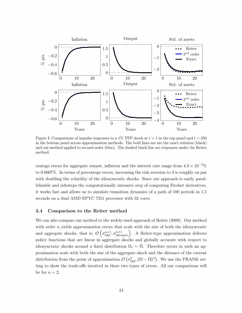
Blue and black solid lines in figure I show the exact and approximate impulse responsesof output, inflation, and asset inequality measured by the standard deviation of individualwealth. They are almost identical in both experiments. The PRANK economy is engineeredin such a way that impulse responses of output and inflation are independent of the assetdistribution, so dynamics of output and inflation are the same in the top and bottom rowsof figure I. This is not the case for other potential variables of interest, such as the dynamicsof asset inequality, as can be seen in the rightmost panels in figure I.

By comparing the two experiments, we can evaluate the precision of our approximationand how the errors deteriorate with the time horizon. In the PRANK economy, we can calcu-late distribution Ωt exactly for all t and the corresponding impulse responses. Our approachcomputes sequential approximations of policy functions and distributions for t = 1, 2, ....Thus, computational errors potentially accumulate over time as we compute responses farinto the future. Because individual wealth follows a random walk process, making any ap-proximation errors accrued by our method permanent, this environment might be a worstcase for testing our approximation method. Despite that, we find that our approximatedistribution is very close to the exact distribution at t = 250 (see online appendix), and wecapture responses of asset inequality to aggregate shock in that period very well.

To document the accuracy and computational speed of our approach we compute ap-proximation errors of our policy functions relative to the true solution and report the resultsin Table I.17 All the errors are reported for a quadratic approximation. The percent errorsrelative to the true solution for the individual consumption policies are less than 0.05% andvary between 0.004%-0.033% as we double volatility of idiosyncratic shocks, while the per-

16This corresponds to a one standard deviation shock to productivity in our baseline economy.17See the online appendix for details of how the approximation errors are computed. Following Den Haan

(2010), we also provide Euler Equation and Dynamic Euler Equation errors.

23

0 10 20−0.6

−0.4

−0.2

0%

pts

Inflation

0 10 20

0

0.5

1

1.5

Output

0 10 20

−2

−1

0

Std. of assets

Reiter2nd orderExact

0 10 20−0.6

−0.4

−0.2

0

Years

%pts

Inflation

0 10 20

0

0.5

1

1.5

Years

Output

0 10 20−4

−3

−2

−1

0

Years

Std. of assets

Reiter2nd orderExact

Figure I: Comparisons of impulse responses to a 1% TFP shock at t = 1 in the top panel and t = 250in the bottom panel across approximation methods. The bold lines are are the exact solution (black)and our method applied to second-order (blue). The dashed black line are responses under the Reitermethod.

centage errors for aggregate output, inflation and the interest rate range from 4.3× 10−5%

to 0.0007%. In terms of percentage errors, increasing the risk aversion to 3 is roughly on parwith doubling the volatility of the idiosyncratic shocks. Since our approach is easily paral-lelizable and sidesteps the computationally intensive step of computing Frechet derivatives,it works fast and allows us to simulate transition dynamics of a path of 100 periods in 1.5seconds on a dual AMD EPYC 7351 processor with 32 cores.

3.4 Comparison to the Reiter method

We can also compare our method to the widely-used approach of Reiter (2009). Our methodwith order n yields approximation errors that scale with the size of both the idiosyncraticand aggregate shocks, that is, O

(σn+1agg , σ

n+1idiosync

). A Reiter-type approximation delivers

policy functions that are linear in aggregate shocks and globally accurate with respect toidiosyncratic shocks around a fixed distribution Ωt = Ω. Therefore errors in such an ap-proximation scale with both the size of the aggregate shock and the distance of the currentdistribution from the point of approximation O

(σ2agg, ‖Ω− Ω‖2

). We use the PRANK set-

ting to show the trade-offs involved in these two types of errors. All our comparisons willbe for n = 2.

24

Maximum Errors (%) Ind. Consumption Agg. Output Inflation Interest Rate

2nd Order

γ = 1, σε = 0.50 0.0039 4.2e-6 3.1e-5 4.3e-5γ = 1, σε = 0.75 0.0134 2.6e-5 1.5e-4 2.2e-4γ = 1, σε = 1.00 0.0328 8.2e-5 4.9e-4 6.9e-4γ = 3, σε = 0.5 0.0453 0.0011 0.0024 0.0034

Reiter-based

γ = 1, σε = 0.50 0.0374 0.0616 0.0337 0.0505γ = 1, σε = 0.75 0.0466 0.0610 0.0335 0.0501γ = 1, σε = 1.00 0.0492 0.0602 0.0329 0.0493γ = 3, σε = 0.5 0.0896 0.2252 0.1327 0.1991

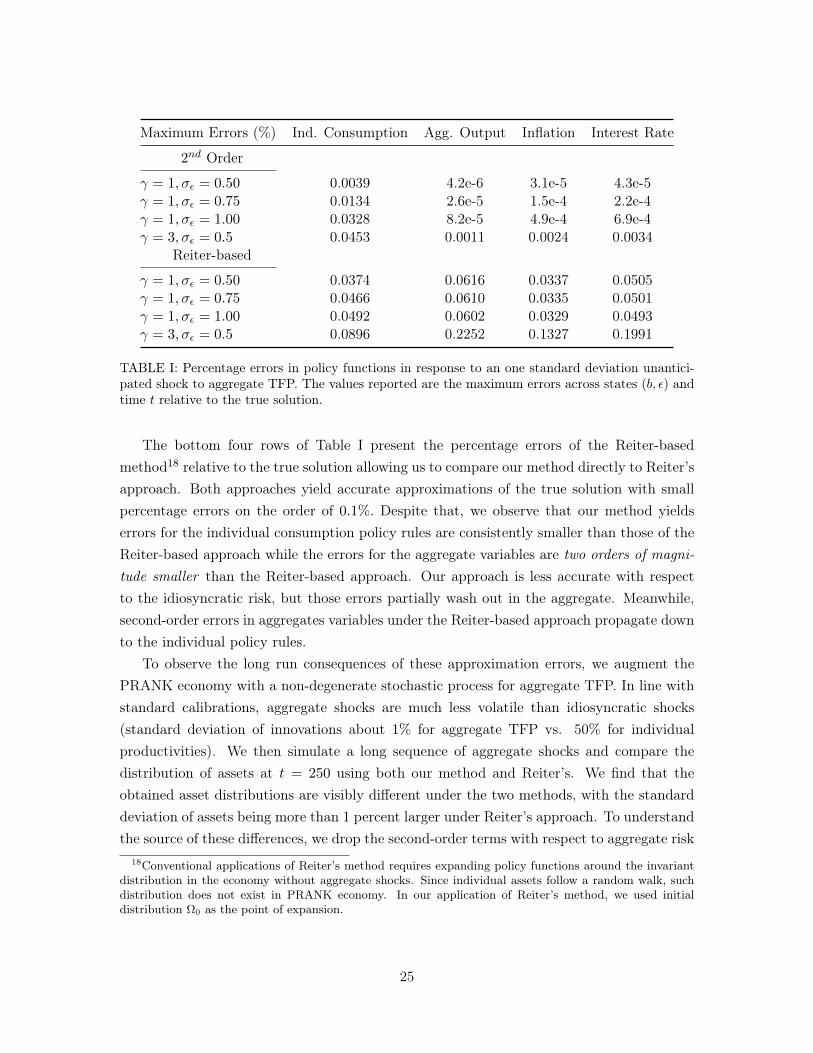
TABLE I: Percentage errors in policy functions in response to an one standard deviation unantici-pated shock to aggregate TFP. The values reported are the maximum errors across states (b, ε) andtime t relative to the true solution.

The bottom four rows of Table I present the percentage errors of the Reiter-basedmethod18 relative to the true solution allowing us to compare our method directly to Reiter’sapproach. Both approaches yield accurate approximations of the true solution with smallpercentage errors on the order of 0.1%. Despite that, we observe that our method yieldserrors for the individual consumption policy rules are consistently smaller than those of theReiter-based approach while the errors for the aggregate variables are two orders of magni-tude smaller than the Reiter-based approach. Our approach is less accurate with respectto the idiosyncratic risk, but those errors partially wash out in the aggregate. Meanwhile,second-order errors in aggregates variables under the Reiter-based approach propagate downto the individual policy rules.

To observe the long run consequences of these approximation errors, we augment thePRANK economy with a non-degenerate stochastic process for aggregate TFP. In line withstandard calibrations, aggregate shocks are much less volatile than idiosyncratic shocks(standard deviation of innovations about 1% for aggregate TFP vs. 50% for individualproductivities). We then simulate a long sequence of aggregate shocks and compare thedistribution of assets at t = 250 using both our method and Reiter’s. We find that theobtained asset distributions are visibly different under the two methods, with the standarddeviation of assets being more than 1 percent larger under Reiter’s approach. To understandthe source of these differences, we drop the second-order terms with respect to aggregate risk

18Conventional applications of Reiter’s method requires expanding policy functions around the invariantdistribution in the economy without aggregate shocks. Since individual assets follow a random walk, suchdistribution does not exist in PRANK economy. In our application of Reiter’s method, we used initialdistribution Ω0 as the point of expansion.

25

from our expansions and re-compute the long run distribution using this inferior approxi-mation. This distribution (which has error of the order O

(σ2agg, σ

3agg

)) is almost identical to

the distribution generated by the Reiter method, which allows us to conclude that ignoringhigher-order effects of aggregate shocks can inject long-run drifts into approximation errors.We report details about this and other related experiments in the online appendix.

The consequences of ignoring movements of Ωt away from Ω can be seen in the responsesof the standard deviation of assets in figure I. While the PRANK economy is constructedso that responses of output and inflation do not depend on the asset distribution at all, theresponses of other moments, such as asset inequality, do depend on it. This implies thatReiter’s approximation of these impulse responses becomes progressively poorer when thedistribution of assets drifts away from the point of approximation. In this example, themovement of the distribution away from the point of approximation is due to idiosyncraticincome risk but similar issues would emerge in economies where aggregate shocks follownon-degenerate stochastic processes for which nonlinear impulse responses would generallydepend on the past history of aggregate shocks or on the current state.

4 Calibration

Our model builds on two literatures – New Keynesian monetary models and Bewely-Huggert-Aiyagari heterogeneous agent models. To focus on the key trade-offs that our Ramseyplanner faces, we keep the baseline economy close to commonly used specifications. Ourinitial calibration ignores some features such as ample heterogeneity in marginal propensitiesto consume and heterogeneous labor earning responses in recessions. We incorporate themas extensions in section 6.

Preferences and technology parameters

We assume that preferences are isoelastic u (c, l) = c1−ν

1−ν −n1+γ

1+γ and set ν = 3, γ = 2. Wecalibrate to annual data and set discount factor β = 0.96. We set Θ = 1 and Φ = 6 toattain average markups of 20%. We abstract from the use of intermediates in productionand set α = 1. We choose the cost of nominal price changes ψ to match the slope of theaggregate Phillips curve. Sbordone (2002) estimates the slope of the U.S. Phillips curveusing quarterly data to be about 0.05. To convert that to an annual frequency we multiplyher number by 4. To a first order approximation the slope of the Phillips curve in our modelis(Φ− 1

)/ψ, which implies ψ = 20.

26

Idiosyncratic and aggregate uncertainty

We assume that all shocks are Gaussian and set the standard deviations of εε,i,t and εθ,i,t to8.7% and 10.3%, and the autocorrelation ρθ =0.992 to match evidence on individual wagedynamics from Low et al. (2010).

The stochastic process for the markup shocks is calibrated so that movements in thelabor share of output are consistent with movements in the U.S. corporate sector’s laborshare (Table 1.14, NIPA) over the period 1947-2016. Calibrated values for (ρΦ, σΦ) are(0.85, 4.6%).19 The stochastic process for aggregate labor productivity, log Θt, is calibratedso that output per hour is consistent with detrended U.S. non-farm real output per hour(BLS) over the period 1947-2016. Calibrated values for (ρΘ, σΘ) are (0.73, 1.23%).

Initial conditions

A common approach in the heterogeneous agent macro-labor literature is to specify gov-ernment policy

(G,Υt, Qt

)and study long-run allocations in an associated competitive

equilibrium. A well-known property of several models in this class is that the invariantdistribution underpredicts the amount of wealth inequality. As we shall see, asset inequal-ity has important implications for optimal policy responses. We calibrate initial conditionsθi,−1, bi,−1, sii to be consistent with empirical distributions of wages, nominal claims, andclaims to real firm profits. In section 5.1.1, we show that the drift from this distribution isslow and its presence matters very little for the optimal policy responses.20

We use the 2007 wave of the Survey of Consumer Finances (SCF) as our benchmark forearnings and asset inequality. We follow the procedure proposed by Doepke and Schneider(2006) to map household-level direct and indirect holdings of financial assets to the jointdistribution of claims to nominal debt and claims to equity.21 Table II reports summarystatistics for our sample. Of particular relevance to results presented in section 5 is thatearnings and assets are positively correlated and that assets inequality is much larger thanearnings inequality.

The final parameter is the level of government expenditures G, which we calibrate tobe consistent with the ratio of non-transfer government expenditures to tax revenues. To

19There is large range of choices for how markup shocks are modeled and calibrated. In the DSGEliterature, for instance, Smets and Wouters (2007), Justiniano et al. (2010), Gali et al. (2007) use ARMA(1,1)processes and estimate the quarterly persistence to be in the range of 0.90–0.95. In the finance literature,for instance, Greenwald et al. (2014) estimate factor share shocks with a monthly persistence of 0.995. Ourcalibrated value for ρΦ = 0.85 lies within the range of these estimates.

20Incorporating proposed “fixes” in the literature to obtain a sufficiently skewed invariant distributionof wealth, for instance allowing persistent shocks to discount factors (Krusell and Smith (1998)), bequests(De Nardi (2004)), entrepreneurial choice (Cagetti and De Nardi (2006)), or persistent idiosyncratic differ-ences in returns to financial assets (Benhabib et al. (2019)), and then computing a Ramsey allocation forsuch an economy is interesting but beyond the scope of this paper.

21The online appendix contains details about how we apply the Doepke and Schneider (2006) procedure.

27

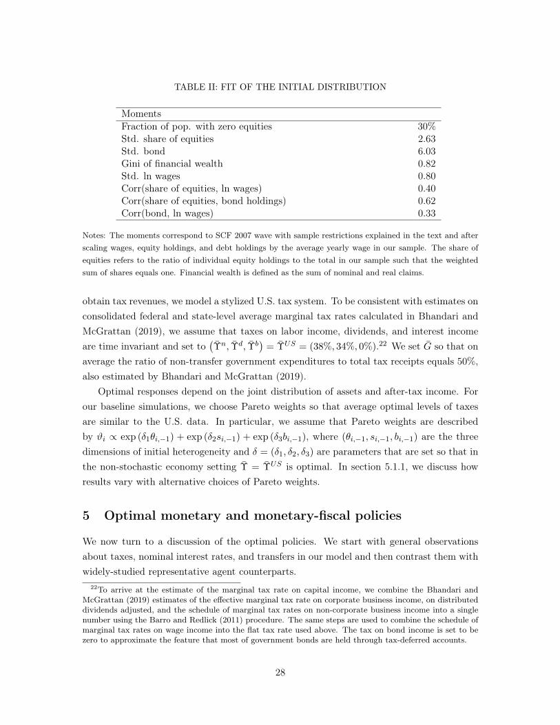
TABLE II: FIT OF THE INITIAL DISTRIBUTION

MomentsFraction of pop. with zero equities 30%Std. share of equities 2.63Std. bond 6.03Gini of financial wealth 0.82Std. ln wages 0.80Corr(share of equities, ln wages) 0.40Corr(share of equities, bond holdings) 0.62Corr(bond, ln wages) 0.33

Notes: The moments correspond to SCF 2007 wave with sample restrictions explained in the text and afterscaling wages, equity holdings, and debt holdings by the average yearly wage in our sample. The share ofequities refers to the ratio of individual equity holdings to the total in our sample such that the weightedsum of shares equals one. Financial wealth is defined as the sum of nominal and real claims.

obtain tax revenues, we model a stylized U.S. tax system. To be consistent with estimates onconsolidated federal and state-level average marginal tax rates calculated in Bhandari andMcGrattan (2019), we assume that taxes on labor income, dividends, and interest incomeare time invariant and set to

(Υn, Υd, Υb

)= ΥUS = (38%, 34%, 0%).22 We set G so that on

average the ratio of non-transfer government expenditures to total tax receipts equals 50%,also estimated by Bhandari and McGrattan (2019).

Optimal responses depend on the joint distribution of assets and after-tax income. Forour baseline simulations, we choose Pareto weights so that average optimal levels of taxesare similar to the U.S. data. In particular, we assume that Pareto weights are describedby ϑi ∝ exp (δ1θi,−1) + exp (δ2si,−1) + exp (δ3bi,−1), where (θi,−1, si,−1, bi,−1) are the threedimensions of initial heterogeneity and δ = (δ1, δ2, δ3) are parameters that are set so that inthe non-stochastic economy setting Υ = ΥUS is optimal. In section 5.1.1, we discuss howresults vary with alternative choices of Pareto weights.

5 Optimal monetary and monetary-fiscal policies

We now turn to a discussion of the optimal policies. We start with general observationsabout taxes, nominal interest rates, and transfers in our model and then contrast them withwidely-studied representative agent counterparts.

22To arrive at the estimate of the marginal tax rate on capital income, we combine the Bhandari andMcGrattan (2019) estimates of the effective marginal tax rate on corporate business income, on distributeddividends adjusted, and the schedule of marginal tax rates on non-corporate business income into a singlenumber using the Barro and Redlick (2011) procedure. The same steps are used to combine the schedule ofmarginal tax rates on wage income into the flat tax rate used above. The tax on bond income is set to bezero to approximate the feature that most of government bonds are held through tax-deferred accounts.

28

The Ramsey planner in our economy has several instruments at their disposal: thenominal interest rates, tax rates on labor income, dividends, and bond income as well aslump-sum transfers. Revenues are raised directly through taxes and indirectly throughnominal interest rates and inflation. These revenues are spent on servicing governmentdebt, paying exogenous expenditures G, and financing transfers. The timing of transfersis undetermined since Ricardian equivalence holds.23 Taxes and inflation that raise theserevenues generate dead-weight losses. Average levels of taxes and transfers depend on theunderlying inequality and on the Pareto weights that appear in the planner’s objectivefunction.

We compare optimal allocations in our baseline setting (to be abbreviated as HANK)to optimal responses in a representative agent version of our model (to be abbreviated asRANK). In RANK, welfare considerations arise from concerns for price stabilization whichare summarized by fluctuations in the rate of inflation, and concerns for output stabilizationwhich are summarized by fluctuations in output relative to its first-best level. To achievethe first best, the planner can set nominal rates equal to the natural rate of interest (thereal rate that prevails in the absence of nominal rigidities), and then implement a subsidyon labor income, Υn

t = −1/Φt to eliminate time-varying markups, financed by a reductionin lump-sum transfers. Such a policy sets the inflation and output gap to zero at all dates,leaving no role for taxes on dividends or bond income.

With heterogeneous agents, such a policy is not optimal. For example, the burdenof transfers falls disproportionately on poor households who finance a large portion of theirconsumption using these transfers. Our HANK setting is designed to match across-householddifferences in shares of labor, dividend, and bond income and, therefore, generates differentialexposures to aggregate shocks. By setting the average level of taxes optimally, the plannerprovides redistribution and some insurance against idiosyncratic risks. However, due toincomplete asset markets, there is also a role for the planner to vary policy with shocks inorder to ensure relative consumption shares are smooth across states and time. Providingthis within-person insurance in response to aggregate shocks is a new force that is absent inRANK.

Adjusting the tax rates on bond and dividend income allows the planner, with minimaldistortions, to influence after-tax real returns and helps in replacing the missing Arrowsecurities. When taxes are fixed, monetary policy has to take up the insurance role. Byvarying nominal rates in response to shocks, the planner can affect real wages, real returns,and therefore provide imperfect insurance.

These optimal responses are conveniently represented in terms of impulse response func-23We explore the optimal timing of transfers in section 6.1 where we extend the model to incorporate

heterogeneity in the marginal propensity to consume.

29

tions, which will be our focus for the rest of the paper. An impulse response of variable Xt

to unexpected shock Ek of size δ in period k is defined as E0 [Xt| Ek = δ] − E0 [Xt| Ek = 0].For simulations, we set size δ to be one standard deviation of E . The responses are time-and state-dependent, and non-linear in the size of the shock.

We begin with the monetary responses to markup shocks and build several insights thatcarry over to the rest of the experiments.

5.1 Monetary policy responses to a markup shock

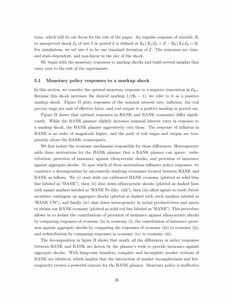
In this section, we consider the optimal monetary response to a negative innovation in EΦ,t.Because this shock increases the desired markup 1/(Φt − 1), we refer to it as a positivemarkup shock. Figure II plots responses of the nominal interest rate, inflation, the realpre-tax wage per unit of effective labor, and real output to a positive markup in period one.

Figure II shows that optimal responses in HANK and RANK economies differ signifi-cantly. While the RANK planner slightly increases nominal interest rates in response toa markup shock, the HANK planner aggressively cuts them. The response of inflation inHANK is an order of magnitude higher, and the path of real wages and output are tem-porarily above the RANK counterparts.

We first isolate the economic mechanism responsible for those differences. Heterogeneityadds three motivations for the HANK planner that a RANK planner can ignore: redis-tribution, provision of insurance against idiosyncratic shocks, and provision of insuranceagainst aggregate shocks. To spot which of these motivations influence policy responses, weconstruct a decomposition by successively studying economies located between HANK andRANK as follows. We (i) start with our calibrated HANK economy (plotted as solid blueline labeled as “HANK”), then (ii) shut down idiosyncratic shocks (plotted as dashed lineswith square markers labeled as “HANK No Idio. risk”), then (iii) allow agents to trade Arrowsecurities contingent on aggregate shocks (plotted as dashed with circle markers labeled as“HANK CM”), and finally (iv) shut down heterogeneity in initial productivities and assetsto obtain our RANK economy (plotted as solid red line labeled as “RANK”). This procedureallows us to isolate the contributions of provision of insurance against idiosyncratic shocksby comparing responses of economy (ii) to economy (i); the contribution of insurance provi-sion against aggregate shocks by comparing the responses of economy (iii) to economy (ii);and redistribution by comparing responses in economy (iv) to economy (iii).

The decomposition in figure II shows that nearly all the differences in policy responsesbetween HANK and RANK are driven by the planner’s wish to provide insurance againstaggregate shocks. With lump-sum transfers, complete and incomplete market versions ofRANK are identical, which implies that the interaction of market incompleteness and het-erogeneity creates a powerful concern for the HANK planner. Monetary policy is ineffective

30

in providing redistribution or insurance against idiosyncratic shocks beyond what can beachieved through taxes Υ. In contrast, monetary policy can provide insurance against ag-gregate shocks because it can act as an imperfect substitute for the missing Arrow securities.

It is easiest to understand the provision of insurance and the differences between RANKand HANK economies by considering a one-time, fully transient positive markup shock.The textbook effect of this shock is an increase in inflationary pressure. Monetary policycan offset that force by depressing marginal costs. Since marginal costs are proportionalto aggregate demand, a contractionary increase in nominal rates is optimal in the RANKeconomy. Galí (2015) dubs this mechanism “leaning against the wind.”

This one-time markup shock also changes the mix of factor payments: it increases div-idends and lowers wages. When household are homogeneous as in the RANK economy, orcan all trade Arrow securities ex-ante, the change in the composition of firms’ payments doesnot affect welfare: agents who mainly receive wage income will hold the portfolio of Arrowsecurities that provide a payoff that offsets the drop in wage income. When the appropriateArrow securities are missing, monetary policy can improve welfare by providing insuranceagainst aggregate shocks. To offset the drop in labor income, the Ramsey planner sets inter-est rates to stimulate real wages. Since real wages are firms’ marginal costs, the monetarypolicy action that provides insurance is opposite to one that promotes price stability.

The net effect of a markup shock on optimal monetary policy depends on the relativestrengths of planner’s price stability and insurance provision motives. The cost of inflationis set by the price adjustment cost parameter ψ while insurance provision motives dependon inequalities in stock ownership relative to inequalities in wage income. If stock holdingsare perfectly aligned with labor earnings, that is, if the share of stocks that each personowns equals his or her share of aggregate labor compensation, then the insurance provisionmotive vanishes; a positive effect on dividends exactly offsets the negative effect on laborearnings. In such a case, optimal responses are similar to those in RANK.24 The reason thatHANK responses in figure II differ so much from what would support price stability is thatstock holdings are much more skewed than labor earnings in U.S. data, making insuranceconcerns strong in our calibration.

Figure II also shows that the most efficient way to provide insurance is to front-loadit: virtually all differences in HANK and RANK optimal outcomes are driven by policies inperiod t = 1. Agents can borrow and lend freely, and as a result, their utility depends on thepresent value of factor payments but not their exact timing. The first-order approximation

24The RANK economy is a special case, where both shares are equal to one, but the same result will holdin the economy with arbitrary heterogeneity so long as shares of dividends and earnings are aligned. Seeonline appendix for an illustration.

31

0 2 4 6 8 10

0

−0.5

%pts

Nominal rate

HANK

HANK No Idio. risk

HANK CM

RANK

0 2 4 6 8 10

0

0.2

Inflation

0 2 4 6 8 10−0.2

0

0.1

Years

%pts

Log output

0 2 4 6 8 10

−0.8

−0.4

0

Years

Wage per unit effective labor

Figure II: Optimal monetary response to a markup shock. The bold blue and red lines are thecalibrated HANK and RANK responses respectively. The dashed black lines with squares andcircles are responses under HANK with idiosyncratic shocks shutdown and with complete markets,respectively.

of firm’s optimality condition (17) can be written as

πt = βEtπt+1 + const · wt + const · (− ln Φt) , (35)

where πt is log inflation, wt is the log deviation of the wage per unit of effective labor fromits average level. Equation (35) shows that inflation in period t is proportional to the presentdiscounted value of future wages. As a consequence, an increase in wage in some period k,increases inflation in all t ≤ k. Therefore, to minimize costs of inflation it is optimal todeliver all the adjustment in the present discounted value of wages at the time of the shock.

The optimal response to a negative markup shock is virtually a mirror image of anoptimal response to a positive markup shock. Averaged over time, the net expected flow ofresources to each agent generated by the monetary policy response is approximately zero; anoutcome consistent with optimal responses driven mainly by the planner’s insurance ratherthan the redistribution motives.

32

5.1.1 Role of key parameters

Optimal responses vary with parameters that change the trade-off between price stabilizationand insurance motives. The magnitude of the price stabilization motive is driven by the valueof the price adjustment cost parameter ψ. The strength of the planner’s insurance motivedepends on the relative post-tax inequality in dividends and labor earnings. The inequality,in turn, depends on the distribution of assets and labor productivities, and on the levels oftaxes Υ that are determined by the choice of Pareto weights. In this section, we study howoptimal monetary policy responses vary with these objects. We report the main findingshere and relegate details to the online appendix.

We set the value for ψ following estimates of Sbordone (2002). In a staggered priceadjustment model, such an estimate would correspond to firms changing prices every ninemonths. Studies using micro evidence on price changes (see Nakamura and Steinsson (2013))recover estimates that range from around 6.8 to 12 months. In the online appendix, we varyψ between half to twice of our baseline value to study the sensitivity of our results withrespect to ψ. We find that that the on-impact change in the nominal rates is fairly similarto the baseline, while the peak response of inflation varies roughly linearly in ψ for thisrange. In addition, we also report a case where we set ψ ≈ 0 to study a benchmark withfully flexible prices.

Next we study sensitivity with respect to Pareto weights. For a wide range of weights,we repeat our decomposition in figure II and show that virtually all the difference betweenHANK and RANK responses are driven by insurance needs. Quantitatively, insurance needsdepend on correlation between individual shares of after-tax labor and dividend incomes.Lower correlations generally imply larger differences between HANK and RANK responses.For Pareto weights that correspond to a fairly large range of taxes around the baseline U.S.levels, impulse responses are quantitatively similar to the baseline responses in figure II.25

Since inequality drifts over time in our economy, optimal responses depend, in principle,on the time t. In our calibrated economy, we found the drift to be slow and thereforeresponses in t = 25 and t = 50 appear very similar to those at t = 1.

25Eliminating inequality in assets, say by a 100% tax on dividends, does not eliminate the need forinsurance. An economy with unequal stock ownership and a 100% tax on dividends is isomorphic to aneconomy without dividend taxes and equal stock ownership. In such an economy, a positive markup shockbenefits agents with low labor earnings (since windfall from profits is greater than their drop in earnings) andhurts high-earners. All households, however, would still prefer to eliminate this risk. In the online appendixwe show that optimal responses of a Utilitarian planner look very similar to those in figure II, although theidentities of the agents who benefit from a positive mark up shock differs from our baseline calibration.

33

5.2 Monetary-fiscal response to a markup shock

We now turn to studying a Ramsey planner who chooses both monetary and fiscal policyactions. Figure III shows optimal responses to a markup shock when the planner choosestax rates in addition to nominal interest rates. The planner offsets the impact of the shockusing a combination of a labor subsidy and a dividend tax while the nominal interest rateis unchanged.

In the RANK economy, lump-sum taxes are non-distortionary, and taxes on dividendand interest income are redundant. Under the optimal monetary-fiscal policy, the plannerachieves the first best by setting Υn

t = −1/Φt to offset monopoly distortions, choosing thepath of nominal rates that delivers a constant price level and setting lump-sum taxes tosatisfy the government’s budget constraint.

In the HANK economy, the burden of lump-sum taxes falls disproportionately on poorhouseholds. The RANK prescription of a proportional labor subsidy financed by reducinglump-sum transfers is therefore not optimal. Instead, the planner finances the labor incomesubsidy using a one-time tax on dividends. This tax exactly offsets the gains to stockowners from the higher markups and thus the policy response provides complete insuranceto all agents with respect to the markup shock. Finally, the flat nominal rate implements aconstant price level.

5.3 Optimal responses to productivity shocks

Figure IV shows optimal monetary response to a negative TFP shock. The monetary re-sponses in HANK differ significantly from RANK, and the decomposition reveals that thedifference is once again driven by the lack of insurance against aggregate shocks.

To understand why the planner wants to provide insurance, first observe that a TFPshock leads to the same reduction in both profits and labor earnings. Thus, firm owners andworkers suffer equally from the shock. The impact of a TFP shock has different effects ondifferent agents because agents are heterogeneous in their bond holdings: agents who holda lot of bonds suffer less from the TFP shock than otherwise identical agents who are indebt. Market incompleteness is the necessary friction that prevents borrowers and saversfrom structuring contracts to provide an effective hedge against TFP shocks. Monetarypolicy fills in this gap by lowering returns on debt which transfers resources from the saversto borrowers and keeps the relative consumption shares smooth.

The optimal policy response departs conceptually from RANK, and more generally, fromthe prescription that monetary policy should aim to minimize fluctuations in inflation andthe New Keynesian concept of an “output gap.” In response to TFP shocks, setting theinterest rate to the “natural level” (a level that would prevail in a flexible price economy)

34

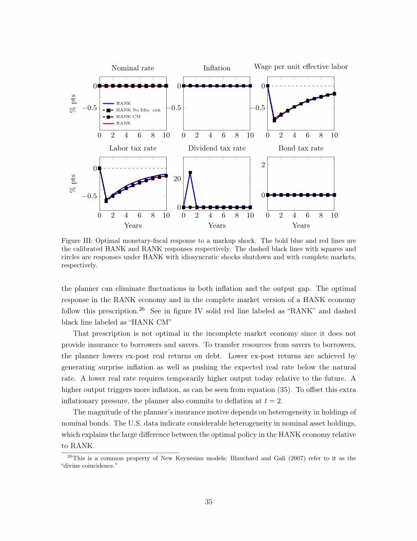
0 2 4 6 8 10

−0.5

0

%pts

Nominal rate

HANK

HANK No Idio. risk

HANK CM

RANK

0 2 4 6 8 10

−0.5

0

Inflation

0 2 4 6 8 10

−0.5

0

Wage per unit effective labor

0 2 4 6 8 10

−0.5

0

Years

%pts

Labor tax rate

0 2 4 6 8 100

20

Years

Dividend tax rate

0 2 4 6 8 10

0

2

Years

Bond tax rate

Figure III: Optimal monetary-fiscal response to a markup shock. The bold blue and red lines arethe calibrated HANK and RANK responses respectively. The dashed black lines with squares andcircles are responses under HANK with idiosyncratic shocks shutdown and with complete markets,respectively.

the planner can eliminate fluctuations in both inflation and the output gap. The optimalresponse in the RANK economy and in the complete market version of a HANK economyfollow this prescription.26 See in figure IV solid red line labeled as “RANK” and dashedblack line labeled as “HANK CM”

That prescription is not optimal in the incomplete market economy since it does notprovide insurance to borrowers and savers. To transfer resources from savers to borrowers,the planner lowers ex-post real returns on debt. Lower ex-post returns are achieved bygenerating surprise inflation as well as pushing the expected real rate below the naturalrate. A lower real rate requires temporarily higher output today relative to the future. Ahigher output triggers more inflation, as can be seen from equation (35). To offset this extrainflationary pressure, the planner also commits to deflation at t = 2.

The magnitude of the planner’s insurance motive depends on heterogeneity in holdings ofnominal bonds. The U.S. data indicate considerable heterogeneity in nominal asset holdings,which explains the large difference between the optimal policy in the HANK economy relativeto RANK.

26This is a common property of New Keynesian models; Blanchard and Gali (2007) refer to it as the“divine coincidence.”

35

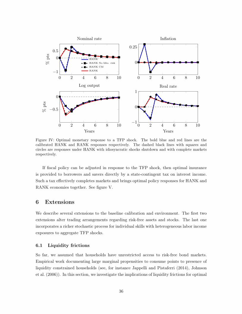
0 2 4 6 8 10

−1

0

0.5%

pts

Nominal rate

HANK

HANK No Idio. risk

HANK CM

RANK

0 2 4 6 8 10

0

0.25

Inflation

0 2 4 6 8 10

−0.5

0

Years

%pts

Log output

0 2 4 6 8 10−1

0

1

Years

Real rate

Figure IV: Optimal monetary response to a TFP shock. The bold blue and red lines are thecalibrated HANK and RANK responses respectively. The dashed black lines with squares andcircles are responses under HANK with idiosyncratic shocks shutdown and with complete marketsrespectively.

If fiscal policy can be adjusted in response to the TFP shock, then optimal insuranceis provided to borrowers and savers directly by a state-contingent tax on interest income.Such a tax effectively completes markets and brings optimal policy responses for HANK andRANK economies together. See figure V.

6 Extensions

We describe several extensions to the baseline calibration and environment. The first twoextensions alter trading arrangements regarding risk-free assets and stocks. The last oneincorporates a richer stochastic process for individual skills with heterogeneous labor incomeexposures to aggregate TFP shocks.

6.1 Liquidity frictions

So far, we assumed that households have unrestricted access to risk-free bond markets.Empirical work documenting large marginal propensities to consume points to presence ofliquidity constrained households (see, for instance Jappelli and Pistaferri (2014), Johnsonet al. (2006)). In this section, we investigate the implications of liquidity frictions for optimal

36

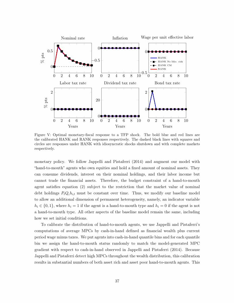
0 2 4 6 8 10

0

0.5

%pts

Nominal rate

0 2 4 6 8 10

−0.5

0

Inflation

0 2 4 6 8 10−0.5

0

Wage per unit effective labor

HANK

HANK No Idio. risk

HANK CM

RANK

0 2 4 6 8 10

0

2

Years

%pts

Labor tax rate

0 2 4 6 8 100

20

Years

Dividend tax rate

0 2 4 6 8 10

0

2

Years

Bond tax rate

Figure V: Optimal monetary-fiscal response to a TFP shock. The bold blue and red lines arethe calibrated HANK and RANK responses respectively. The dashed black lines with squares andcircles are responses under HANK with idiosyncratic shocks shutdown and with complete marketsrespectively.

monetary policy. We follow Jappelli and Pistaferri (2014) and augment our model with“hand-to-mouth” agents who own equities and hold a fixed amount of nominal assets. Theycan consume dividends, interest on their nominal holdings, and their labor income butcannot trade the financial assets. Therefore, the budget constraint of a hand-to-mouthagent satisfies equation (2) subject to the restriction that the market value of nominaldebt holdings PtQtbi,t must be constant over time. Thus, we modify our baseline modelto allow an additional dimension of permanent heterogeneity, namely, an indicator variablehi ∈ 0, 1, where hi = 1 if the agent is a hand-to-mouth type and hi = 0 if the agent is nota hand-to-mouth type. All other aspects of the baseline model remain the same, includinghow we set initial conditions.

To calibrate the distribution of hand-to-mouth agents, we use Jappelli and Pistaferri’scomputations of average MPCs by cash-in-hand defined as financial wealth plus currentperiod wage minus taxes. We put agents into cash-in-hand quantile bins and for each quantilebin we assign the hand-to-mouth status randomly to match the model-generated MPCgradient with respect to cash-in-hand observed in Jappelli and Pistaferri (2014). BecauseJappelli and Pistaferri detect high MPCs throughout the wealth distribution, this calibrationresults in substantial numbers of both asset rich and asset poor hand-to-mouth agents. This

37

approach also preserves the distribution of real and nominal claims of the baseline modelwhich results in the same insurance motives and, therefore, allows us to distinguish effectscoming from the ‘liquidity frictions’ of the hand-to-mouth agents.27

Figures VI and VII show optimal monetary responses to markup and aggregate TFPshocks for the calibration with hand-to-mouth agents and compares them to optimal re-sponses in the baseline calibration. Evidently, the trading frictions that give rise to the het-erogeneities in MPCs make the paths for nominal rates, real wages, and inflation smootherthan they are in the baseline model. Since Ricardian equivalence no longer holds, the opti-mal path of transfers is now uniquely pinned down. We show next that the deviation of theoptimal policy responses from those in our baseline model are driven by the inability of thehand-to-mouth agents to borrow and save to smooth their consumption over time as well asthe substantial heterogeneity within the set of liquidity constrained households.

We start with optimal monetary policy responses to a markup shock in figure VI. In thebaseline calibration (solid blue line), the planner provides insurance against the shock byfront-loading higher wages and avoiding additional future inflation from firms anticipatinghigher future marginal costs. That front-loading policy would be costly for hand-to-mouthagents – they would have too much income in the short run relative to future which theycannot smooth over time. Thus, in addition to providing insurance, the planner must alsoensure that the consumption paths of the hand-to-mouth agents are smooth over time.

A natural way to both achieve insurance and to allow for smoother consumption after theshock would be to set the timing of lump-sum transfers appropriately. However, the planneris confronted with the problem that hand-to-mouth agents are not homogeneous. A path oftransfers that would smooth the consumption of poor hand-to-mouth agents reliant on wageincome would exacerbate the volatility of consumption of rich hand-to-mouth agents whorely mostly on dividend income. Thus, heterogeneity among liquidity constrained agentsmakes transfers a less effective tool.28

In addition to picking an appropriate path for transfers, the planner distorts allocationsto induce a smoother path (dashed black line) for the real wage. A smoother path of real

27Our specification and calibration is also in line with Kaplan et al. (2014) and Kaplan et al. (2018) whoemphasize that data indicate substantial heterogeneity among liquidity constrained agents. Their baselinecalibration assigns higher MPCs to agents having low liquid wealth. In their calibration, about two thirds ofagents who have zero liquid wealth nevertheless have positive illiquid wealth. Our specification captures bothfeatures of their calibration because our high-s hand-to-mouth agents behave like the wealthy hand-to-mouthagents in Kaplan et al. (2018).

28To highlight this point and isolate the role of wealthy hand-to-mouth, in the online appendix, we consideran alternative calibration in which the bottom 15% of the cash-in-hand distribution is set to be hand-to-mouth. This example captures the flavor of typical calibrations of a one-asset-Aiyagari model becausethe constrained hand-to-mouth agents are more homogeneous and depend almost entirely on their laborincomes. We show that the dynamics of interest rates, inflation, output and wages is almost identical to thatof the baseline economy with no liquidity frictions. When liquidity-constrained agents are homogeneous, theplanner can effectively borrow on their behalf and use transfers to smooth their consumption.

38

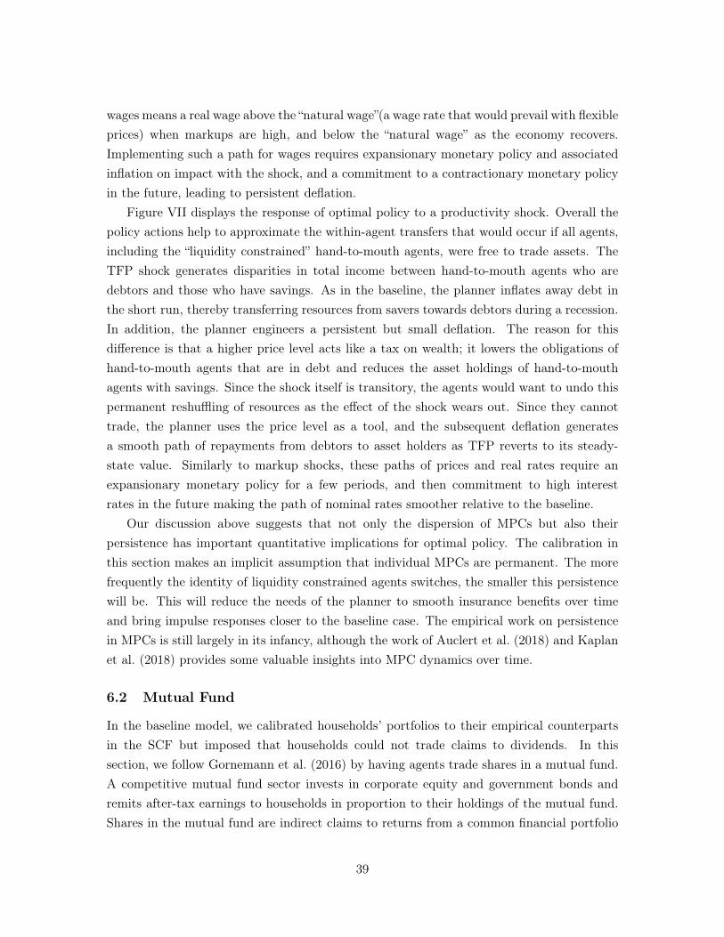
wages means a real wage above the “natural wage”(a wage rate that would prevail with flexibleprices) when markups are high, and below the “natural wage” as the economy recovers.Implementing such a path for wages requires expansionary monetary policy and associatedinflation on impact with the shock, and a commitment to a contractionary monetary policyin the future, leading to persistent deflation.

Figure VII displays the response of optimal policy to a productivity shock. Overall thepolicy actions help to approximate the within-agent transfers that would occur if all agents,including the “liquidity constrained” hand-to-mouth agents, were free to trade assets. TheTFP shock generates disparities in total income between hand-to-mouth agents who aredebtors and those who have savings. As in the baseline, the planner inflates away debt inthe short run, thereby transferring resources from savers towards debtors during a recession.In addition, the planner engineers a persistent but small deflation. The reason for thisdifference is that a higher price level acts like a tax on wealth; it lowers the obligations ofhand-to-mouth agents that are in debt and reduces the asset holdings of hand-to-mouthagents with savings. Since the shock itself is transitory, the agents would want to undo thispermanent reshuffling of resources as the effect of the shock wears out. Since they cannottrade, the planner uses the price level as a tool, and the subsequent deflation generatesa smooth path of repayments from debtors to asset holders as TFP reverts to its steady-state value. Similarly to markup shocks, these paths of prices and real rates require anexpansionary monetary policy for a few periods, and then commitment to high interestrates in the future making the path of nominal rates smoother relative to the baseline.

Our discussion above suggests that not only the dispersion of MPCs but also theirpersistence has important quantitative implications for optimal policy. The calibration inthis section makes an implicit assumption that individual MPCs are permanent. The morefrequently the identity of liquidity constrained agents switches, the smaller this persistencewill be. This will reduce the needs of the planner to smooth insurance benefits over timeand bring impulse responses closer to the baseline case. The empirical work on persistencein MPCs is still largely in its infancy, although the work of Auclert et al. (2018) and Kaplanet al. (2018) provides some valuable insights into MPC dynamics over time.

6.2 Mutual Fund

In the baseline model, we calibrated households’ portfolios to their empirical counterpartsin the SCF but imposed that households could not trade claims to dividends. In thissection, we follow Gornemann et al. (2016) by having agents trade shares in a mutual fund.A competitive mutual fund sector invests in corporate equity and government bonds andremits after-tax earnings to households in proportion to their holdings of the mutual fund.Shares in the mutual fund are indirect claims to returns from a common financial portfolio

39

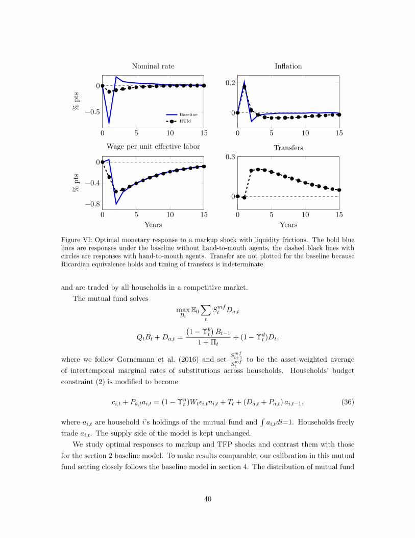
0 5 10 15

−0.5

0

%pts

Nominal rate

Baseline

HTM

0 5 10 15

0

0.2

Inflation

0 5 10 15

−0.8

−0.4

0

Years

%pts

Wage per unit effective labor

0 5 10 15

0

0.3

Years

Transfers

Figure VI: Optimal monetary response to a markup shock with liquidity frictions. The bold bluelines are responses under the baseline without hand-to-mouth agents, the dashed black lines withcircles are responses with hand-to-mouth agents. Transfer are not plotted for the baseline becauseRicardian equivalence holds and timing of transfers is indeterminate.

and are traded by all households in a competitive market.The mutual fund solves

maxBt

E0

∑t

Smft Da,t

QtBt +Da,t =

(1−Υb

t

)Bt−1

1 + Πt+ (1−Υd

t )Dt,

where we follow Gornemann et al. (2016) and set Smft+1

Smftto be the asset-weighted average

of intertemporal marginal rates of substitutions across households. Households’ budgetconstraint (2) is modified to become

ci,t + Pa,tai,t = (1−Υnt )Wtεi,tni,t + Tt + (Da,t + Pa,t) ai,t−1, (36)

where ai,t are household i’s holdings of the mutual fund and∫ai,tdi=1. Households freely

trade ai,t. The supply side of the model is kept unchanged.We study optimal responses to markup and TFP shocks and contrast them with those

for the section 2 baseline model. To make results comparable, our calibration in this mutualfund setting closely follows the baseline model in section 4. The distribution of mutual fund

40

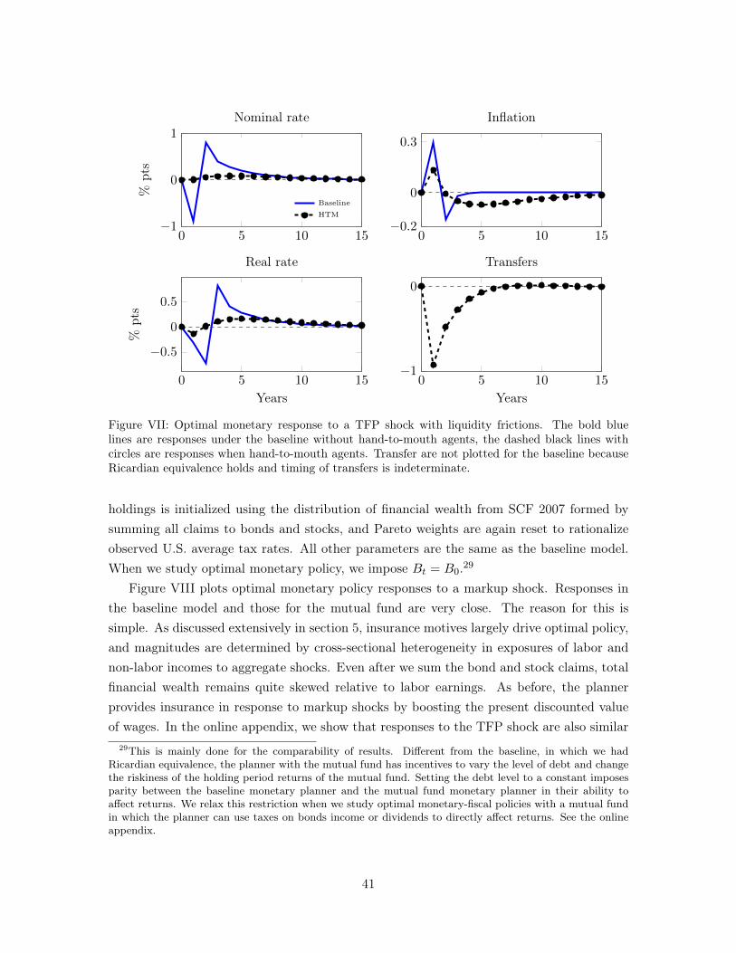
0 5 10 15−1

0

1%

pts

Nominal rate

Baseline

HTM

0 5 10 15−0.2

0

0.3

Inflation

0 5 10 15

−0.5

0

0.5

Years

%pts

Real rate

0 5 10 15−1

0

Years

Transfers

Figure VII: Optimal monetary response to a TFP shock with liquidity frictions. The bold bluelines are responses under the baseline without hand-to-mouth agents, the dashed black lines withcircles are responses when hand-to-mouth agents. Transfer are not plotted for the baseline becauseRicardian equivalence holds and timing of transfers is indeterminate.

holdings is initialized using the distribution of financial wealth from SCF 2007 formed bysumming all claims to bonds and stocks, and Pareto weights are again reset to rationalizeobserved U.S. average tax rates. All other parameters are the same as the baseline model.When we study optimal monetary policy, we impose Bt = B0.29

Figure VIII plots optimal monetary policy responses to a markup shock. Responses inthe baseline model and those for the mutual fund are very close. The reason for this issimple. As discussed extensively in section 5, insurance motives largely drive optimal policy,and magnitudes are determined by cross-sectional heterogeneity in exposures of labor andnon-labor incomes to aggregate shocks. Even after we sum the bond and stock claims, totalfinancial wealth remains quite skewed relative to labor earnings. As before, the plannerprovides insurance in response to markup shocks by boosting the present discounted valueof wages. In the online appendix, we show that responses to the TFP shock are also similar

29This is mainly done for the comparability of results. Different from the baseline, in which we hadRicardian equivalence, the planner with the mutual fund has incentives to vary the level of debt and changethe riskiness of the holding period returns of the mutual fund. Setting the debt level to a constant imposesparity between the baseline monetary planner and the mutual fund monetary planner in their ability toaffect returns. We relax this restriction when we study optimal monetary-fiscal policies with a mutual fundin which the planner can use taxes on bonds income or dividends to directly affect returns. See the onlineappendix.

41

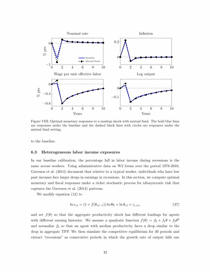
0 2 4 6 8 10

0

−1

%pts

Nominal rate

Baseline

Mutual Fund

0 2 4 6 8 10

0

0.2

Inflation

0 2 4 6 8 10

−0.8

−0.4

0

Years

%pts

Wage per unit effective labor

0 2 4 6 8 10

−0.1

0

Years

Log output

Figure VIII: Optimal monetary responses to a markup shock with mutual fund. The bold blue linesare responses under the baseline and the dashed black lines with circles are responses under themutual fund setting.

to the baseline.

6.3 Heterogeneous labor income exposures

In our baseline calibration, the percentage fall in labor income during recessions is thesame across workers. Using administrative data on W2 forms over the period 1978-2010,Guvenen et al. (2014) document that relative to a typical worker, individuals who have lowpast incomes face larger drops in earnings in recessions. In this section, we compute optimalmonetary and fiscal responses under a richer stochastic process for idiosyncratic risk thatcaptures the Guvenen et al. (2014) patterns.

We modify equation (12) to

ln εi,t = (1 + f(θi,t−1)) ln Θt + ln θi,t + εε,i,t, (37)

and set f(θ) so that the aggregate productivity shock has different loadings for agentswith different earning histories. We assume a quadratic function f(θ) = f0 + f1θ + f2θ

2

and normalize f0 so that an agent with median productivity faces a drop similar to thedrop in aggregate TFP. We then simulate the competitive equilibrium for 30 periods andextract “recessions” as consecutive periods in which the growth rate of output falls one

42

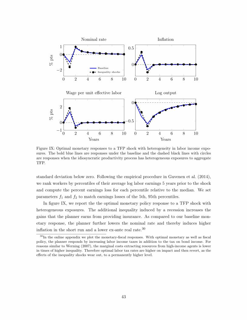
0 2 4 6 8 10

−2

0

1%

pts

Nominal rate

Baseline

Inequality shocks

0 2 4 6 8 10

0

0.5

Inflation

0 2 4 6 8 10−1

0

2

Years

%pts

Wage per unit effective labor

0 2 4 6 8 10

−0.5

0

Years

Log output

Figure IX: Optimal monetary responses to a TFP shock with heterogeneity in labor income expo-sures. The bold blue lines are responses under the baseline and the dashed black lines with circlesare responses when the idiosyncratic productivity process has heterogeneous exposures to aggregateTFP.

standard deviation below zero. Following the empirical procedure in Guvenen et al. (2014),we rank workers by percentiles of their average log labor earnings 5 years prior to the shockand compute the percent earnings loss for each percentile relative to the median. We setparameters f1 and f2 to match earnings losses of the 5th, 95th percentiles.

In figure IX, we report the the optimal monetary policy response to a TFP shock withheterogeneous exposures. The additional inequality induced by a recession increases thegains that the planner earns from providing insurance. As compared to our baseline mon-etary response, the planner further lowers the nominal rate and thereby induces higherinflation in the short run and a lower ex-ante real rate.30

30In the online appendix we plot the monetary-fiscal responses. With optimal monetary as well as fiscalpolicy, the planner responds by increasing labor income taxes in addition to the tax on bond income. Forreasons similar to Werning (2007), the marginal costs extracting resources from high-income agents is lowerin times of higher inequality. Therefore optimal labor tax rates are higher on impact and then revert, as theeffects of the inequality shocks wear out, to a permanently higher level.

43

7 Concluding Remarks

Our paper makes two contributions. It develops a way to approximate optimal plans ineconomies with heterogeneous agents, and reevaluates lessons for monetary and fiscal policydrawn from New Keynesian economies. Relative to price stability motives that typicallydrive policy prescriptions, heterogeneity adds a quantitatively important insurance motive.We developed these insights using a fairly canonical setting that combined the most basicversions of the new Keynesian model and the incomplete market models. Our methods canbe extended to environments that feature a more detailed modeling of household balancesheets, richer labor market dynamics including realistic wage-setting frictions, and richerasset markets formulations that are consistent with the observed returns and monetarytransmission channels. We suspect that insurance concerns with respect to aggregate shocksand determinants of heterogeneous income exposures in the cross section will still be key inunderstanding policy responses. What will change with these features are the details of howthis insurance is implemented. Cataloging this is left for future work.

44

References

Acharya, Sushant, and Keshav Dogra. 2018. “Understanding HANK: Insights from aPRANK.” FRB of New York Staff Report(835): .

Aiyagari, S. Rao, Albert Marcet, Thomas J. Sargent, and Juha Seppala. 2002.“Optimal Taxation without State-Contingent Debt.” Journal of Political Economy, 110(6):1220–1254.

Anderson, Evan W, Lars Peter Hansen, and Thomas J Sargent. 2012. “Smallnoise methods for risk-sensitive/robust economies.” Journal of Economic Dynamics andControl, 36(4): 468–500.

Auclert, Adrien, Matthew Rognlie, and Ludwig Straub. 2018. “The IntertemporalKeynesian Cross.” Working Paper 25020, National Bureau of Economic Research.

Barro, Robert J. 1979. “On the Determination of the Public Debt.” Journal of PoliticalEconomy, 87(5): 940–971.

Barro, Robert J., and Charles J. Redlick. 2011. “Macroeconomic Effects From Gov-ernment Purchases and Taxes.” Quarterly Journal of Economics, 126(1): 51–102.

Benhabib, Jess, Alberto Bisin, and Mi Luo. 2019. “Wealth Distribution and SocialMobility in the US: A Quantitative Approach.” American Economic Review, 109(5): 1623–47.

Bhandari, Anmol, David Evans, Mikhail Golosov, and Thomas Sargent. 2017.“Fiscal Policy and Debt Management with Incomplete Markets.” Quarterly Journal ofEconomics, 132(2): 617–663.

Bhandari, Anmol, and Ellen McGrattan. 2019. “Sweat Equity in U.S. Private Busi-ness.”

Bilbiie, Florin O. 2019. “Monetary Policy and Heterogeneity: An Analytical Framework.”Unpublished manuscript.

Bilbiie, Florin Ovidiu, and Xavier Ragot. 2017. “Optimal Monetary Policy and Liquid-ity with Heterogeneous Households.” CEPR Discussion Papers 11814, C.E.P.R. DiscussionPapers.

Blanchard, Olivier, and Jordi Gali. 2007. “Real Wage Rigidities and the New KeynesianModel.” Journal of Money, Credit and Banking, 39 35–65.

45

Cagetti, Marco, and Mariacristina De Nardi. 2006. “Entrepreneurship, Frictions, andWealth.” Journal of Political Economy, 114(5): 835–870.

Challe, Edouard. 2017. “Uninsured Unemployment Risk and Optimal Monetary Policy.”Working Papers 2017-54, Center for Research in Economics and Statistics.

Chari, V. V., and Patrick J. Kehoe. 1999. “Chapter 26 Optimal fiscal and monetarypolicy.” In Handbook of macroeconomics. eds. by John B Taylor of Macroeconomics, andMichael Woodford B T Handbook, Volume 1,: Elsevier, 1671–1745.

Childers, David. 2018. “On the Solution and Application of Rational Expectations Modelswith Function-Valued States.” Unpublished manuscript.

De Nardi, Mariacristina. 2004. “Wealth Inequality and Intergenerational Links.” TheReview of Economic Studies, 71(3): 743–768.

Debortoli, Davide, and Jordi Gali. 2017. “Monetary Policy with Heterogeneous Agents:Insights from TANK models.” working papers, Department of Economics and Business,Universitat Pompeu Fabra.

Den Haan, Wouter J. 2010. “Comparison of solutions to the incomplete markets modelwith aggregate uncertainty.” Journal of Economic Dynamics and Control, 34(1): 4 – 27,Computational Suite of Models with Heterogeneous Agents: Incomplete Markets andAggregate Uncertainty.

Doepke, Matthias, and Martin Schneider. 2006. “Inflation and the Redistribution ofNominal Wealth.” Journal of Political Economy, 114(6): 1069–1097.

Evans, David. 2015. “Perturbation Theory with Heterogeneous Agents: Theory and Ap-plications.” Ph.D. dissertation, New York University.

Farhi, Emmanuel. 2010. “Capital Taxation and Ownership When Markets Are Incom-plete.” Journal of Political Economy, 118(5): 908–948.

Fleming, Wendell H. 1971. “Stochastic Control for Small Noise Intensities.” SIAM Journalon Control, 9(3): 473–517.

Fleming, Wendell H, and PE Souganidis. 1986. “Asymptotic series and the method ofvanishing viscosity.” Indiana University Mathematics Journal, 35(2): 425–447.

Galí, Jordi. 2015. Monetary policy, inflation, and the business cycle: an introduction tothe new Keynesian framework and its applications.: Princeton University Press.

46

Gali, Jordi, Mark Gertler, and J. David Lopez-Salido. 2007. “Markups, Gaps, andthe Welfare Costs of Business Fluctuations.” The Review of Economics and Statistics,89(1): 44–59.

Gornemann, Nils, Keith Kuester, and Makoto Nakajima. 2016. “Doves for the Rich,Hawks for the Poor? Distributional Consequences of Monetary Policy.” InternationalFinance Discussion Papers 1167, Board of Governors of the Federal Reserve System (U.S.).

Greenwald, Daniel L, Martin Lettau, and Sydney C Ludvigson. 2014. “Origins ofStock Market Fluctuations.” Working Paper 19818, National Bureau of Economic Re-search.

Guvenen, Fatih, Serdar Ozkan, and Jae Song. 2014. “The Nature of CountercyclicalIncome Risk.” Journal of Political Economy, 122(3): 621–660.

Huggett, Mark. 1993. “The risk-free rate in heterogeneous-agent incomplete-insuranceeconomies.” Journal of Economic Dynamics and Control, 17(5): 953–969.

Jappelli, Tullio, and Luigi Pistaferri. 2014. “Fiscal Policy and MPC Heterogeneity.”American Economic Journal: Macroeconomics, 6(4): 107–36.

Johnson, David S., Jonathan A. Parker, and Nicholas S. Souleles. 2006. “HouseholdExpenditure and the Income Tax Rebates of 2001.” American Economic Review, 96(5):1589–1610.

Judd, Kenneth L, and Sy-Ming Guu. 1993. “Perturbation solution methods foreconomic growth models.” In Economic and Financial Modeling with Mathematica R©.:Springer, 80–103.

Judd, Kenneth L, and Sy-Ming Guu. 1997. “Asymptotic methods for aggregate growthmodels.” Journal of Economic Dynamics and Control, 21(6): 1025–1042.

Justiniano, Alejandro, Giorgio E. Primiceri, and Andrea Tambalotti. 2010. “In-vestment shocks and business cycles.” Journal of Monetary Economics, 57(2): 132 – 145.

Kaplan, Greg, Benjamin Moll, and Giovanni L. Violante. 2018. “Monetary PolicyAccording to HANK.” American Economic Review, 108(3): 697–743.

Kaplan, Greg, Giovanni L Violante, and Justin Weidner. 2014. “The Wealthy Hand-to-Mouth.” Working Paper 20073, National Bureau of Economic Research.

Krusell, Per, and Anthony A Smith, Jr. 1998. “Income and wealth heterogeneity inthe macroeconomy.” Journal of Political Economy, 106(5): 867–896.

47

Legrand, Francois, and Xavier Ragot. 2017. “Optimal policy with heterogeneous agentsand aggregate shocks : An application to optimal public debt dynamics.”Technical report.

Low, Hamish, Costas Meghir, and Luigi Pistaferri. 2010. “Wage risk and employmentrisk over the life cycle.” American Economic Review, 100(4): 1432–1467.

Luenberger, David G. 1997. Optimization by Vector Space Methods. New York, NY, USA:John Wiley & Sons, Inc., , 1st edition.

Marcet, Albert, and Ramon Marimon. 2019. “Recursive Contracts.” Econometrica,87(5): 1589–1631.

Nakamura, Emi, and Jon Steinsson. 2013. “Price Rigidity: Microeconomic Evidenceand Macroeconomic Implications.” Annual Review of Economics, 5(1): 133–163.

Nuno, Galo, and Carlos Thomas. 2016. “Optimal monetary policy with heterogeneousagents.” Working Papers 1624.

Phillips, Kerk L. 2017. “Solving and simulating unbalanced growth models using lineariza-tion about the current state.” Economics Letters, 151 35–38.

Reiter, Michael. 2009. “Solving heterogeneous-agent models by projection and perturba-tion.” Journal of Economic Dynamics and Control, 33(3): 649–665.

Rotemberg, Julio J. 1982. “Monopolistic Price Adjustment and Aggregate Output.” Re-view of Economic Studies, 49(4): 517–531.

Sbordone, Argia M. 2002. “Prices and unit labor costs: a new test of price stickiness.”Journal of Monetary Economics, 49(2): 265–292.

Schmitt-Grohe, Stephanie, and Martin Uribe. 2004a. “Optimal fiscal and monetarypolicy under sticky prices.” Journal of Economic Theory, 114(2): 198–230.

Schmitt-Grohe, Stephanie, and Martin Uribe. 2004b. “Solving dynamic general equi-librium models using a second-order approximation to the policy function.” Journal ofEconomic Dynamics and Control, 28(4): 755–775.

Siu, Henry E. 2004. “Optimal Fiscal and Monetary Policy with Sticky Prices.” Journal ofMonetary Economics, 51(3): 575–607.

Smets, Frank, and Rafael Wouters. 2007. “Shocks and frictions in US business cycles:A Bayesian DSGE approach.” American Economic Review, 97(3): 586–606.

48

Storesletten, Kjetil, Chris I Telmer, and Amir Yaron. 2001. “How important areidiosyncratic shocks? Evidence from labor supply.” American Economic Review, 91(2):413–417.

Werning, Ivan. 2007. “Optimal Fiscal Policy with Redistribution,.” Quarterly Journal ofEconomics, 122(August): 925–967.

Woodford, Michael. 2003. Interest and prices.: Princeton University Press.

49

Online Appendix

A Additional details for section 3

In this section, we fill in the missing steps for section 3. First we show, in the context ofthe section 3.1 economy, how our method extends to higher-order approximations. Second,we show how to generalize the expansions so that we can deal with persistent aggregate andidiosyncratic shocks as well as additional state variables, as discussed in section 3.2.

A.1 Higher order approximations for section 3.1

We start with a second-order approximation to the model presented in section 3.1. Theseare given by

X(Ω, σE;σ) =X + σ(XEE + Xσ

)+

1

2σ2(XEE .(E,E) + 2XEσE + Xσσ

)+O(σ3),

where the symbol a · (b, c) denotes a bilinear map.31 A similar expansion can be written forx(z,Ω, σε, σE;σ).

To obtain the necessary terms, we proceed in two steps: section A.1.1 computes inter-mediate terms including higher-order Frechet derivatives for individual and aggregate policyfunctions, and section A.1.2 uses these terms to compute the second-order expansion. Al-though the second-order expansion requires additional notation, the steps below highlightways in which the same fundamental insights presented in section 3 maintain the tractabilityof the problem.

31Specifically, if a is a n1 × n2 × n3 tensor, b is a n2 × n4 matrix and c is a n3 × n5 matrix thend = a · (b, c) is n1 × n4 × n5 tensor defined by

dilm =∑j,k

aijkbjlckm.

This definition generalizes to when a, b, or c is infinite dimensional, such as with ∂xz.

1

A.1.1 Intermediate terms for second-order expansions

Differentiating equation (22) twice with respect to z we find

0 =Fx−xzz + Fxxzz + Fx+ (xzz + xzpxzz)

+ Fzz + Fzx− · (I, xz) + Fzx · (I, xz) + Fzx+ · (I,xz)

+ Fx−z · (xz, I) + Fx−x− · (xz, xz) + Fx−x · (xz, xz) + Fx−x+ · (xz,xz)

+ Fxz · (xz, I) + Fxx− · (xz, xz) + Fxx · (xz, xz) + Fxx+ · (xz,xz)

+ Fx+z · (xz, I) + Fx+x− · (xz, xz) + Fx+x · (xz, xz) + Fx+x+ · (xz,xz),

where I represents the identity matrix and we use a · (b, c) to denote a bilinear map. Lines 2-5appear complicated but are actually simply combining all of the already known derivatives of xwith cross derivatives of F. It will prove convenient to combine all of these terms into a single term:∑α,β∈z,x−,x,x+ Fαβ · (αz, βz) with the knowledge that zz ≡ I, x−z ≡ xz, and x+

z ≡ xz. In doingthis xzz can be represented by a simple linear equation

xzz = −[Fx− + Fx + Fx+ (I + xzp)

]−1

∑α,β∈z,x−,x,x+

Fαβ · (αz, βz)

.

In a similar manner one can show that

∂xz ·∆ = −[Fx− + Fx + Fx+ (I + xzp)

]−1

∑

α ∈ z,x−,x,x+β ∈ x−,x,x+,X

Fαβ ·(αz, ∂β ·∆

),

where we use ∂x− ·∆ ≡ ∂x+ ·∆ ≡ ∂x ·∆.The last of the derivatives with respect to the state variables that are required for the second

order expansion is ∂2x·(∆1,∆2).We will use the pre computed expressions for ∂x and ∂X evaluating

them in the directions ∆1 and ∆2. Differentiating (22) we find

0 =Fx−∂2x · (∆1,∆2) + Fx∂

2x · (∆1,∆2) + Fx+

(∂2x · (∆1,∆2) + xzp∂2x · (∆1,∆2)

)+ FX∂

2X · (∆1,∆2)

+∑

α,β ∈ x−,x,x+,X

Fαβ ·(∂α ·∆1, ∂β ·∆2

).

In solving this equation for ∂2x · (∆1,∆2) we find

∂2x · (∆1,∆2) = A(z,∆1,∆2) + C(z)∂2X · (∆1,∆2)

2

where

A(z,∆1,∆2) = −[Fx− + Fx + Fx+ (I + xzp)

]−1

∑α,β ∈ x−,x,x+,X

Fαβ ·(∂α ·∆1, ∂β ·∆2

)from terms already known and C(z) is the same term computed in section 3.1. To find∂2X · (∆1,∆2) we differentiate (23) to find

0 =Rx

∫∂2x(y) · (∆1,∆2)dΩ(y) + RX∂

2X · (∆1,∆2) +

∫ ∑α,β∈x(y),X

Rαβ · (∂α ·∆1, ∂β ·∆2) dΩ(y)

+ Rx

∫∂x(y) ·∆1d∆2(y) + Rx

∫∂x(y) ·∆2d∆1(y).

Plugging in for ∂2x · (∆1,∆2) yields a linear equation which can be easily solved for ∂2X ·(∆1,∆2).

A.1.2 Second-order expansions

We can use these derivatives to compute the second-order terms. To find xεε, differentiateF twice with respect to ε to get the linear equation32

0 = Fxxεε + Fx+xzpxεε +∑

α,β∈x,x+,ε

Fαβ ·(αε, βε

),

where x+ε ≡ xzpxε and εε ≡ I. Similarly, xεE solves the following linear equation

0 = FxxεE + Fx+xzpxεE +∑

α∈x,x+,εβ∈x,x+,X,E

Fαβ ·(αε, βE

),

with the understanding that EE ≡ I and x+E ≡ xzpxE + ∂x · ΩE .

Differentiating twice with respect to E yields

0 =FxxEE + Fx+

(xzpxEE + ∂x · ΩEE

)+ FXXEE

+ Fx+

(xzz · (pxE , pxE) + ∂xz · (pxE , ΩE) + ∂xz · (ΩE , pxE) + ∂2x · (ΩE , ΩE)

)(38)

+∑

α,β∈x,x+,X,E

Fαβ · (αE , βE)

32For parsimony we have dropped the dependence on z when not necessary.

3

and ∫RxxEE(y) + RXXEE +

∑α,β∈x(y),X

Rαβ · (αE , βE)dΩ(y). (39)

All the terms in the second line can be computed from our analysis of the previous sectionand all the terms in the third line are known. What remains is to find xEE and XEE . Thisrequires us extend the steps we used in the proof of theorem 1.

Differentiating (24) twice with respect to E , evaluated at σ = 0, yields

ΩEE(y) =−∫ ∑

i

δ(zi − yi)∏j 6=i

ι(zj − yj)ziEE(z)dΩ(z)

−∫ ∑

i

δ′(zi − yi)∏j 6=i

ι(zj − yj)[ziE(z)

]2dΩ(z)

+

∫ ∑i

δ(zi − yi)∑j 6=i

δ(zj − yj)∏k 6=i,j

ι(zk − yk)zjE(z)ziE(z)dΩ(z).

The density is then

ωEE(y) =∂nz

∂y1∂y2 · · · ∂ynzΩEE(y) = −

∑i

∂

∂yi(ziEE(y)ωE(y)

)+∑i

∑j

∂2

∂yi∂yj

(ziE(y)zjE(y)ωE(y)

).

The identical steps to (1) then show that

∂x(z) · ΩEE = C(z)∂X · ΩEE ≡ C(z)X ′EE

with

X ′EE = −(Rx

∫C(y)dΩ(y) + RX

)−1

Rx

(∫xz(y)pxEE(y) + xzz(y) · (pxE , pxE) dΩ(y)

).

(40)As with XE , rather than solving for xEE(z) and XEE jointly, we substitute for ∂x(z) · ΩEEin (38) and solve for xEE(z) yielding the linear relationship

xEE(z) = D1(z) ·[XEE X ′EE

]ᵀ+ D2(z)

where D1(z) is identical to the D1 in section 3.1. We then use this relationship to substituteinto equations (39) and (40) to find XEE and X ′EE .

A key part of the second-order approximations is capturing the effect of risk via theterms xσσ(z) and Xσσ(z).33 Let Cε ≡ Eεᵀε and CE ≡ EEᵀE be the variance-covariancematrix of the idiosyncratic and aggregate shocks respectively. Differentiating (22) and (23)

33It is easy to verify that the cross derivatives with shocks and σ are zero.

4

yields34

0 = Fx− (xεε · Cε + xEE · CE)+Fxxσσ+FXXσσ+Fx+

(xεε·Cε+xEE ·CE+xzpxσσ+∂x·Ωσσ

)(41)

and0 = Rx

∫xσσ(y) + xεε(y) · CεdΩ(y) + RXXσσ. (42)

Before this set of equations can be solved for xσσ, we must evaluate Ωσσ. Differentiating(24) and evaluating at σ = 0 yields

Ωσσ(y) =−∫ ∑

i

δ(zi − yi)∏j 6=i

ι(zj − yj)(ziσσ(z) + ziεε · Cε

)dΩ(z)

−∫ ∑

i

δ′(zi − yi)∏j 6=i

ι(zj − yj)[ziε(z)

]2 · CεdΩ(z)

+

∫ ∑i

δ(zi − yi)∑j 6=i

δ(zj − yj)∏k 6=i,j

ι(zk − yk)(zjε(z)ziε(z)

)· CεdΩ(z)

which gives

ωσσ(y) =−∑i

∂

∂yi((ziσσ(y) + ziεε(y) · Cε

)ω(y)

)+∑i

∑j

∂2

∂yi∂yj((ziε(y)zjε(y)

)· Cεω(y)

).

Following the identical steps as theorem (1) to show that show that

∂x(z) · Ωσσ = C(z)∂X · Ωσσ ≡ C(z)X ′σσ

with

X ′σσ =−(Rx

∫C(y)dΩ(y) + RX

)−1

Rx

∫ (xz(y)p (xσσ(y) + xεε(y) · Cε)

+ xzz(y) · (pxε, pxε) · Cε

)dΩ(y). (43)

We then substitute for ∂x · Ωσσ = C(z)X ′σσ in (41) to and solve for xσσ(z) to find the34If a is a n1 × n2 × n2 tensor and C is a n2 × n2 matrix then d = a ·C is length n1 vector defined

bydi =

∑j,k

aijkCjk.

5

linear relationshipxσσ(z) = E0(z) + E1(z)

[Xσσ X ′σσ

]ᵀ.

This relationship can then be plugged into (42) and (43) to yield a linear equation for Xσσ

and X ′σσ.

A.2 Expansions in the general case of section 3.2

We extend our method to handle persistent shocks and other endogenous persistent statevariables besides the distributional state Ω. To do so, we extend the equilibrium conditionsin the following manner

F(E−x, x,E+x, X,Λ,Θ, ε,E, z

)= 0, (44)

which must hold for all z in the support of Ω,

R

(∫xdΩdPr(ε), X,E+X,Λ,Θ,E

)= 0, (45)

and a first-order vector autoregression model Θ′ = ρΘΘ + (1− ρΘ)Θ +E for the exogenousshocks. The law of motion of the distribution is given by

Ω (Ω,Λ,Θ,E) (z) =

∫ι (z (y,Ω,Λ,Θ, ε,E) ≤ z) dPr (ε) dΩ (y) ∀z. (46)

We consider a family of perturbations indexed by a positive scalar σ that scales all shocksε,E so that the policy functions are X(Ω,Λ,Θ, σE;σ) and x(z,Ω,Λ,Θ, σε, σE;σ). We willuse · to denote these functions evaluated at σ = 0.

Unlike section 3.1, we cannot assume that Ω(Ω,Λ,Θ) is stationary but we recover theindependence property

Lemma 2. For any Ω,Λ,Θ, the policy functions z(z,Ω,Λ,Θ) satisfy ∂z(z,Ω,Λ,Θ) = 0

for all z and zz(z,Ω,Λ,Θ) independent of z.

Proof. We proceed similar to the proof of Lemma 1 in the main text. The first ordercondition with respect to bi,t−1 yields

E[

[c (z,Ω,Λ,Θ, ·, ·)]−ν

1 + Π (Ω,Λ,Θ, ·, )(µ− µ (z,Ω,Λ,Θ, ·, ·))

]= 0.

When σ = 0, this yields µ(z,Ω,Λ,Θ) = µ for all z. While equation (20) to the zeroth order

6

is

Q(Ω,Λ,Θ)M(Ω,Λ,Θ)m = m (z,Ω,Λ,Θ) M(Ω(Ω,Λ,Θ)

) (1 + Π

(Ω(Ω,Λ,Θ)

))−1.

By construction, the Pareto-Negishi weights integrate to one which implies m (z,Ω,Λ,Θ) =

m for all z. Finally, the law of motion for θ implies

θ (z,Ω,Λ,Θ) = ρθθ.

Together they imply ∂z(z,Ω,Λ,Θ) = 0 for all z and zz(z,Ω,Λ,Θ) independent of z.

A by product of 2 is that zz is diagonal. Although we exploit this property in the nextsection it is not essential.

We start by showing how our expansion extends to the transition path. We assumefor a given Ω,Λ,Θ we have solved for the σ = 0 transition dynamics Ωn, Λn, ΘnNn=0

with (Ω0, Λ0, Θ0) = Ω,Λ,Θ and (ΩN , ΛN , ΘN ) = (Ω, Λ, Θ) at a non-stochastic steadystate. Solving the the transition dynamics is eased by the fact that we know, a priori, thetransition dynamics of Ω. For the remainder of this appendix we use ·n to denote derivativesevaluated at (Ωn, Λn, Θn) and, to save on notation, and use · to denote derivatives evaluatedat the steady state (ΩN , ΛN , ΘN ). We’ll start by showing how to compute derivatives atthe steady state and then show how to evaluate derivatives along the path.

The policy rules for X and x can then be approximated via Taylor expansion. The firstorder expansions for these variables are given by

X(Ω,Λ,Θ, σE;σ) = X0 + σ(X0EE + X0

σ) +O(σ2)

andx(z,Ω,Λ,Θ, σε, σE;σ) = x0(z) + σ

(x0ε(z)ε+ x0

E(z)E + x0σ(z)

)+O(σ2).

For brevity, we present the necessary derivatives for the first order expansions. Higher orderterms extend analogously to section A.1 .

A.2.1 Derivatives at the steady state

The derivatives of the policy functions with respect to Λ and Θ as well as the Frechetderivative with respect to the distribution Ω are used repeatedly in what follows.

Differentiating (44) with respect to Λ yields (lemma 2 implies that ΩΛ = 0).

Fx−(z)xΛ(z) + Fx(z)xΛ(z) + Fx+(z)(xΛ(z)ΛΛ

)+ FX(z)XΛ = 0

7

andRx

∫xΛ(z)dΩ(z) + RXXΛ + RX+XΛΛΛ + RΛ = 0.

The object ΛΛ is unknown. It requires solving a nonlinear equation which we show belowcan be expressed using operations that involve matrices of small dimension. First note that

xΛ(z) = −(Fx−(z) + Fx(z) + ΛΛFx+(z))−1FX(z)XΛ

Let A(z) = −(Fx−(z) + Fx(z) + ΛΛFx+(z))−1FX(z), then

XΛ = −(Rx

∫A(z)dΩ(z) + RX + ΛΛRX+

)−1

RΛ.

Let P be such that Λ = PX. Therefore, ΛΛ must solve

ΛΛ = −P

(Rx

∫A(z)dΩ(z) + RX + ΛΛRX+

)−1

RΛ.

This can be found easily with a 1-dimensional root solver as all the matrices that need tobe inverted are small dimensional.

Next differentiating (44) with respect to Θ yields (lemma 2 implies that ΩΘ = 0).

Fx−(z)xΘ(z) + Fx(z)xΘ(z) + Fx+(z)(xΘ(z)ρΘ + xΛ(z)PXΘ

)+ FX(z)XΘ + FΘ(z) = 0.

This yields a linear equation in xΘ and XΘ which we can solve for xΘ.35 Plugging in forthe linear relationship between xΘ and XΘ in

Rx

∫xΘ(z)dΩ(z) + RXXΘ + RX+XΘρΘ + RX+XΛPXΘ + RΘ = 0.

yields a linear equation for XΘ.

Finally to determine the Frechet derivative, we differentiate (44) along the direction ∆.Doing so yields

(Fx−(z) + Fx(z)

)∂x(z)·∆+Fx+(z)∂x(z)·∂Ω·∆+Fx+(z)xΛ(z)P∂X ·∆+FX(z)∂X ·∆ = 0.

We first derive an analogue of the property ∂Ω ·∆ = ∆. This holds in the simple section 3.1economy but fails in the more general case. We proceed by showing that we can evaluate∂Ω along a direction ∆j that satisfies the property that there exists a function a(·) such

35Easiest to exploit ρΘ =

(ρΘ 00 ρΦ

)and solve for each column of xΘ separately.

8

that the density of ∆j takes the form

∂

∂yj(a(y)ω(y))

Begin by differentiating the law of motion for Ω at σ = 0. Since ∂z = 0, we get

(∂Ω ·∆j)(y) =

∫ ∏i

ι(zi(z) ≤ yi) ∂

∂zj(a(z)ω(z)) dz

=

∫ ∑i

δ(zi(z)− yi)∏k 6=i

ι(zk(z) ≤ yk)∂zi

∂zj(z)a(z)ω(z)dz.

= zjz

∫δ(zj − yj)

∏k 6=j

ι(zk ≤ yk)a(z)ω(z)dz

where the second line was achieved through integration by parts. The third line was achievedby noting that ω is the density of the steady state so z(z) = z for all z in its support andexploiting that ∂zi

∂zj(z) is both independent of z and diagonal. We can also compute the

density of (∂Ω ·∆j)(y) by applying the derivative ∂nz

∂y1∂y2···∂ynz which gives

zjz∂

∂yj

∫ ∏k

δ(zk − yk)a(z)ω(z)dz = zjz∂

∂yj(a(y)ω(y)) .

We conclude that ∂Ω ·∆j = zjz∆j .

Evaluating the Frechet derivative of (44) in this particular direction ∆j we find

(Fx−(z) + Fx(z) + Fx+(z)xzp + zjzFx+(z)

)∂x(z)·∆j+Fx+(z)xΛ(z)P∂X·∆j+FX(z)∂X·∆j = 0.

Solving for ∂x(z) ·∆j we conclude that36

∂x(z) ·∆j = −(Fx−(z) + Fx(z) + Fx+(z)xzp + zjzFx+(z)

)−1 (Fx+(z)xΛ(z)P + FX(z)

)∂X ·∆j

≡ Cj(z)∂X ·∆j .

Taking the derivative of R along this direction we get

∂X ·∆j = −(Rx

∫Cj(z)dΩ(z) + RX+(zjzI + XΛP) + RX

)−1

Rx

∫x(z)d∆j(z)

≡(Dj)−1

Rx

∫x(z)d∆j(z).

36For generality we have written this as one value of C for each individual state, i.e. Cj . In fact, one onlyneeds one value for each level of zjz which in our case is two: 1 and ρθ.

9

From the definition of ∆j , we can use integration by parts to find that

∂X ·∆j =(Dj)−1

Rx

∫xzj (z)a(z)dΩ(z).

A.2.2 Expansion along the path

We will use the derivatives of the state variables at the end of the transition path to evaluateour expansion along the path using backward induction. This approach is recursive, so we’llcompute the derivatives at (Ωn, Λn, Θn) assuming derivatives at period n+1 of the transitionare known.

Differentiating (44) and (45) with respect to Λ we obtain

Fnx−(z)xnΛ(z) + Fnx (z)xnΛ(z) + Fnx+(z)xn+1Λ (z)PXn

Λ + FX(z)XnΛ = 0

andRnx

∫xnΛ(z)dΩ(z) + RnXX

nΛ + RnX+X

n+1Λ PXn

Λ + RnΛ = 0.

As both xn+1Λ (z) and Xn+1

Λ are already known we can solve for xnΛ(z) to find

xnΛ(z) = −(Fnx−(z) + Fnx(z)

)−1(Fnx+(z)xn+1

Λ (z)P + FnX(z))Xn

Λ,

and, therefore, XnΛ equals

−(−Rnx

∫ (Fnx−(z) + Fnx(z)

)−1(Fnx+(z)xn+1

Λ (z)P + FnX(z))dΩ(z) + RnX + RnX+X

n+1Λ P

)−1

RnΛ

Differentiating with respect to Θ we find

Fnx−(z)xnΘ(z)+Fnx (z)xnΘ(z)+Fnx+(z)(xn+1

Θ (z)ρΘ + xn+1Λ (z)PXn

Θ

)+FnX(z)Xn

Θ+FnΘ(z) = 0.

This yields a linear equation in xnΘ and XnΘ which we can solve for xnΘ as a linear function

of XnΘ. Plugging in for the linear relationship between xnΘ and Xn

Θ in

Rnx

∫xnΘ(z)dΩ(z) + RnXX

nΘ + RnX+X

n+1Θ ρΘ + RX+X

n+1Λ PXn

Θ + RnΘ = 0

yields a linear equation that can be solved for XnΘ.

To compute the Frechet derivative, we’ll evaluate the derivative in direction ∆j,n withdensity of the form

∂

∂yj(an(y)ωn(y))

where ωn is the density of Ωn and an(y) is some arbitrary function. For this derivative we

10

find

(∂Ωn ·∆j,n)(y) =

∫ ∏i

ι(zi(z) ≤ yi) ∂

∂zj(an(z)ωn(z)) dz

=

∫ ∑i

δ(zi(z)− yi)∏k 6=i

ι(zk(z) ≤ yk)∂zi,n

∂zj(z)an(z)ωn(z)dz.

= zjz

∫δ(zi(z)− yj)

∏k 6=j

ι(zi(z) ≤ yk)an(z)ωn(z)dz.

The density of (∂Ωn ·∆j,n)(y) is found by applying the derivative ∂nz

∂y1∂y2···∂ynz to get

zjz∂

∂yj

∫ ∏k

δ(zk − yk)an(z)ωn(z)dz = zjz∂

∂yj(an+1(y)ωn+1(y)

),

where an+1(y) = an(z−1(y)).We conclude therefore that ∂Ωn ·∆j,n = zjz∆j,n+1 were we ac-knowledge the implicit relationship between ∆j,n and ∆j,n+1 through an+1(y) = an(z−1(y)).

The Frechet derivative of F then is

(Fnx−(z) + Fnx (z)

)∂xn(z) ·∆j,n + zjzFx+(z)∂xn+1(z) ·∆j,n+1

+Fnx+(z)xn+1Λ (z)P∂Xn ·∆j,n + FX(z)∂X ·∆j,n = 0.

Since the previous equation is recursive in ∂xn(z) ·∆j,n, we can solve it forward to obtain

∂xn(z) ·∆j,n =

N−n∑k=0

Cj,nk (z)∂Xn+k ·∆j,n+k

with Cj,N0 defined from Cj in the previous section and

Cj,n0 (z) = −(Fnx−(z) + Fnx (z)

)−1 (Fnx+(z)xn+1

Λ (z)P + FX(z))

Cj,nk (z) = −zjz(Fnx−(z) + Fnx (z)

)−1Cj,n+1k−1 (z).

Similarly, differentiating R generates

Rnx

∫∂xn(z) ·∆j,ndΩn(z) + zjzR

nX+∂X

n+1 ·∆j,n+1 + Xn+1Λ P∂Xn ·∆j,n)

+RnX(z)∂Xn ·∆j,n + Rnx

∫xn(z)d∆j,n(z) = 0

11

Substituting for ∂xn(z) ·∆j,n yields a recursive equation with solution

∂Xn ·∆j,n = −(Dj,n

)−1

(Rnx

∫xn(z)d∆j,n +

N−n∑k=1

Ej,nk ∂Xn+k ·∆j,n+k

)

with Dj,N defined by Dj in the previous section and

Dj,n = Rnx(z)

∫Cj,n0 (z)dΩn(z) + RnX+X

n+1Λ P + RnX

andEj,nk = Rnx

∫Cj,nk (z)dΩn(z) + 1k=1z

jzR

nX+.

Finally we can use this knowledge to solve for XE . We’ll give expressions for X0E all

others are analogous. Differentiating with respect to E yields

F0x(z)x0

E(z)+ F0x+(z)

(x1

Θ(z) + x1z(z)px0

E(z) + ∂x1(z) · Ω0E + x1

Λ(z)PX0E)

+ F0X(z)X0

E + F0E(z) = 0.

(47)In order to proceed, we need to determine Ω0

E . Differentiating the law of motion of Ω gives

Ω0E = −

∑j

∫δ(zj(z)− yj)

∏i

ι(zi(z) ≤ yi)zj,0E (z)ω0(z)dz.

The density of Ω0E is therefore

−∑j

∂

∂yj

∫ ∏i

δ(zi(z)− yi)zj,0E (z)ω0(z)dz = −∑j

∂

∂yj

(zj,0E

(z−1(y)

)ω1(y)

)≡∑j

ω0,j,1E ,

where 1 here represents that the objects are evaluated using the density of the transition path attime 1, ω1(y). If we define Ω0,j,n

E as the measure with density

ω0,j,nE (y) = − ∂

∂yj

zj,0E

z−1(. . . z−1(y)

)︸ ︷︷ ︸n times

ωn(y)

,

then

∂x1(z) · Ω0,j,1E =

N−1∑k=0

Cj,1k (z)∂X1+k · Ω0,j,1+kE ≡

N−1∑k=0

Cj,1k X′j,1+kE .

Combined with (47) gives a linear system

M0(z)x0E(z) = N0(z)

[I X ′

1,1E X ′

2,1E . . . X ′

nz,NE

]ᵀ

12

and which can be solved for x0E(z). To find X ′j,nE , we note that they satisfy the equation

X ′j,nE = −

(Dj,n

)−1

Rnzj + Rnx

∫ xnzj (z)zj,0E

z−1(. . . z−1(z)

)︸ ︷︷ ︸n times

dΩn(z) +

N−n∑k=1

Ej,nk X ′j,n+kE

.

Combining the previous equation with

R0x

∫x0E(z)dΩ0(z) + R0

XX0E + R0

X+

(X1

Θ + X1E + X1

ΛPX0E)

+ R0E = 0

yields a linear system

O ·[X0

E X ′1,1E X ′

2,1E . . . X ′

nz,NE

]ᵀ= P

which can be solved for X0E .

The term x0ε(z) satisfies

x0ε(z) =

(F 0x(z) + F 0

x+(z)x1z(z(z))p

)−1F 0ε (z).

A.2.3 An Alternative Approximation

In this section we present the alternative approach highlighted in section 3.2 where we scaleσE, σε, σΘ, σθ and expand with respect to σ instead of just σE, σε.

For this approach, the full policy function forX can be written as X(Ω(σ),Λ, σΘ, σE;σ)

where Ω(y;σ) incorporates the fact that we are scaling θ with σ and therefore also scalingΩ. Formally, we have (assuming the simplest case where m,µ and θ are the only individualstate variables for our problem)

Ω(y;σ) =

∫ι(m ≤ y1)ι(µ ≤ y2)ι(σθ ≤ y3)dΩ(m,µ, θ). (48)

The same proof can be used toshow that Lemma 2 holds for this approximation as well.There still may be transition dynamics with respect to Λ, at which point it will be necessaryto follow sections A.2.1 and A.2.2 to compute the relevant derivatives for the expansion.37

X and x can then be approximated using Taylor expansions with respect to σ. Forbrevity we only report the first order expansion of X which given by

X(Ω(σ),Λ, σΘ, σE;σ) = X0 + σ(∂X0 · Ωσ + X0ΘΘ + X0

EE + X0σ) +O(σ2).

37In the case where there is no endogenous aggregate sate variable only section A.2.1 is required.

13

To obtain ∂X · Ωσ, we differentiate (48) with respect to σ to obtain

Ωσ(y) = −∫ι(m ≤ y1)ι(µ ≤ y2)δ(0− y3)θdΩ(m,µ, θ).

The density of this object is constructed by applying the derivative ∂3

∂y1∂y2∂y3to get

ωσ(y) =− ∂

∂y3

(∫δ(m− y1)δ(µ− y2)δ(0− y3)θdΩ(m,µ, θ)

)=− ∂

∂y3

(δ(0− y3)

∫ω(y1, y2, θ)θdθ

)=− ∂

∂y3(Eθ(y1, y2)ω(y))

where in the last equality we defined Eθ(y1, y2) =∫ω(y1,y2,θ)θdθ∫ω(y1,y2,θ)dθ

as the cross-sectional meanof θ conditional on (m,µ) = (y1,y2). From this expression, we know that ∂X0 · Ωσ can besolved for in the same manner as ∂X0 · Ω0

E using the tools in section (A.2.2).

A.2.4 Simulation and Clustering

To simulate an optimal policy at each date with N agents, we discretize the distributionacross agents with K grid points that we find each period using a k-means clustering al-gorithm. Let ziNi=1 represent the current distribution of agents. The k-means algorithmgenerates K points zkKk=1 with each agent i assigned to a cluster k(i) to minimize thesquared error

∑i ‖zi − zk(i)‖2. We let Ω represent the distribution of N agents and Ω

represent our approximating distribution of clusters.38 At each history, we compute Ω andthen apply our algorithm to approximate the optimal policies around Ω.39 When K = N

we exactly approximate around Ω, but for K < N we can speed up the computations by afactor of NK .

A.2.5 Solving the t = 0 problem

For the Ramsey problem (21), optimality conditions at t = 0 are different from t ≥ 1.The full set of optimality conditions are represented by expanding equations (22)–(24). Wedescribe how to apply our procedure for the section 3.1 simple case. The extension to thegeneral problem in section 2 is straightforward.

We start with some notation. Let ΩB be a measure over the claims to risk-free debt.Denote the t = 0 aggregate policy functions as X0

(ΩB,E0

)and individual policy functions

38Formally Ω(z) has density∑i

1Nδ(z − zi) while Ω(z) has density

∑i

1Nδ(z − zk(i)).

39Similar to section (A.2.3) this is done by constructing a distribution Ω(σ) with density∑i

1Nδ(z−zk(i)−

σ(zi − zk(i))) and then computing ∂X0 · Ωσin the same manner as section (A.2.3).

14

as x0

(b,ΩB, ε0,E0

). Augment the system (22)–(24) with mappings F0 and R0, capturing

the time 0 first order conditions, such that

F0

(x0,E+x, X0, ε0,E0, b0

)= 0 (49)

R0

(∫x0dΩB, X0,E0

)= 0 (50)

Policy functions for t ≥ 1 individual states z0 = (m0, µ0) are components of x0. Let functionΩ0

(ΩB,E0

)map the initial condition ΩB and aggregate shock E0 to a measure Ω over z

using

Ω0

(ΩB,E0

)(z) =

∫ι(z0

(y,ΩB, ε0,E0

)≤ z

)dPr (ε0) dΩB (y) ∀z (51)

Section 3.1 characterizes the small-noise approximations of the t ≥ 1 policy functionsaround an arbitrary Ω. We update Ω along the path by iterating between an approximationand a simulation step. At some t ≥ 1, taking as input Ωt−1, we draw idiosyncratic shocksε for each agent as well as aggregate shocks E , and use the policy functions approximatedaround Ωt−1 to move to the next period Ωt. All that remains to be specified is how thet = 1 state, Ω0, is obtained. We do that below by constructing small-noise approximationsto t = 0 policy functions: X0(ΩB, σE0;σ) and x0(b,ΩB, σε0, σE0;σ). We present a firstorder expansion. Higher order expansions along the lines of A.1 are analogous.

1. Zeroth-order: For some choice of ΩB, the σ = 0 allocation consists of x0(b), x(b) forb in support of ΩB as well as

X0, X

such that

F0

(x0, x, X0, 0, 0, b0

)= 0, R0

(∫x0(b)dΩB(b), X0,E0

)= 0

F(x, x, x, X, 0, 0, z

)= 0, R

(∫x(b)dΩB(b), X, 0

)= 0

2. To compute derivativesx0,ε(b), x0,E(b), x0,σ(b), X0,E , X0,σ

, we use the formulas

from section (A.2.2). The expressions that appear in section (A.2.2) use superscriptn to denote the period of transition path for the σ = 0 allocation. We can obtainx0,ε(b), x0,E(b), x0,σ(b), X0,E , X0,σ

by using those formulas after replacing F 0

• withF0,• , Fn• with F• for n ≥ 1 and similarly for R0

• and Rn• .

3. Simulation: Draw idiosyncratic shocks ε0 for each agent as well as aggregate shocksE0 and use the approximations to policy functions

X0(ΩB, σE0;σ) = X0 + σ(X0,EE0 + X0,σ

)+O(σ2)

15

and

x(b,ΩB, σε0, σE0;σ) = x0(b) + σ (x0,ε(b)ε0 + x0,E(b)E0 + x0,σ(b)) +O(σ2)

to obtain the Ω0(z0) for t = 1.

A.3 Additional details for section 3.3

In this section, we provide more details concerning Acharya and Dogra (2018) “PRANK”economy, which we use as a laboratory to test the accuracy of our algorithm and compare it toalternative methods. We start with equilibrium conditions, next we discuss the calibration,and report the accuracy tests for our method. Finally, we present a simplified version ofthis economy for which we can solve for all gradients in closed form.

Equilibrium in the PRANK economy To obtain the PRANK setting we imposethe following assumptions: (i) labor is supplied inelastically, and period utility functionU(ct, nt) = − exp(−γct), (ii) the distribution of shares is uniform, (iii) Idiosyncratic produc-tivity shocks are i.i.d, and (iv) All tax rates are constant and the monetary policy follows aTaylor rule given by

Q−1t − 1 = a0 (1 + Πt)

a1 (52)

In the PRANK economy, a perfect foresight equilibrium is constructed as follows. For asequence of innovations to TFP EΘ,sTs=0, Agent is consumption ci,t satisfies

ci,t = Ct + µt

(bi,t−1

1 + Πt+ yi,t

), (53)

where yi,t = (1 − Υt)Wtεi,tni,t + Tt + di,t is the households income at date t. The twoparameters Ct and µt that are common to all agents are given by

µt =µt+1

(Qt

1+Πt+1

)1 + µt+1

(Qt

1+Πt+1

) (54)

Ct[1 + µt+1

(Qt

1 + Πt+1

)]= −1

γlnβ

(Qt

1 + Πt+1

)+ Ct+1 + µt+1yt+1 −

γµ2t+1σ

2y,t+1

2(55)

where yt+1 =∫yi,t+1di is the average household income, and σ2

y,t+1 is the variance inhousehold level income. A perfect foresight equilibrium can by solving equations (52)–(55)along with equations (8), (10),(17), and (18).

We check the accuracy of our approximations using an exact solution to the perfectforesight equilibrium. Section (A.3) discusses how we calibrate the PRANK economy, section

16

(A.3) and (A.3) compare approximation errors using several diagnostics.

Calibration We study several cases. For the parameters that are common across thesecases we use Acharya and Dogra (2018) targets which are are quite standard in the repre-sentative agent New Keynesian literature. The discount rate β to 0.96 to get a real rate of4% per year, the elasticity of substitution parameter, Φ, to 6 to target an average markup of20%. The share of intermediate inputs α, is set to 0.6 to target a labor income share of 2/3,and we set the adjustment cost parameter ψ to 41.6 to target a slope of the Phillips curveof 0.06. Aggregate productivity follows an AR(1) process with a decay parameter 0.73, andthe standard deviation of the innovation is set to 1.23% to be consistent with de trendedoutput per hour and we turn off the markup shocks. For the Taylor rule parameters, we seta1 = 1.5 and choose a0 to target 0% inflation rate in absence of aggregate risk. We vary thestandard deviation of idiosyncratic risk, σε ∈0.5, 0.75, 1, and the risk aversion parameter,γ ∈ 1, 3. Our calibrationscover a range that includes Acharya and Dogra (2018) as well aswhat we use in our baseline section 4. Since the distribution of assets is non-stationary, weset Ω0(b) to be Gaussian and calibrate the parameters to be consistent with the distributionof wealth in the SCF. For simulation, we approximate the distribution with 150 points andthe idiosyncratic shocks with 10 point Gaussian quadrature.

Diagnostics In this section, we compare the accuracy of our policy functions in twosettings. We start with a stationary environment with no aggregate risk and study the policyfunction for individual consumption as well as values for the aggregate variables. Then, westudy impulse responses of several aggregate variables to a TFP shock. As mentioned before,the advantage of PRANK is that in both cases, the true solution can be solved for exactly.

We report three types of approximation errors for the individual policy functions: (i)% gap in the approximated and true policies (ii) % gap in the approximated and policyrules implied by the Euler equation (or the Euler equation errors) and (iii) dynamic EulerEquation errors from Den Haan (2010). The first two errors are acquired from the formulas40

Epolc,t (b, ε) ≡ 100× |cTruet (b, ε)− capprxt (b, ε)|

Ct(56)

EEEc,t (b, ε) ≡ 100× |cimpt (b, ε)− capprxt (b, ε)|

Ct, (57)

40As CARA preference feature an aversion to absolute risk and, possibly, negative consumption we reportthe absolute errors scaled by average consumption.

17

where cTruet (b, ε) are constructed using the exact solution and cimpt (b, ε) is defined as

cimpt (b, ε) = − 1

αlog

(β

QtEt[

1

1 + πt+1exp(−αcapproxt+1 (b′, ε′))

]).

The dynamic Euler equation errors are constructed by simulating an alternative series bt andct, for a group of agents, derived using the budget constraint and cimpt evaluated at bt−1. Wethen compare to ct simulated using capprxt and the same sequence of shocks. These errorshave the advantage of allowing for the possibility of small errors accumulating into largeerrors over time. We denote them as EdynEEc,t (b, ε). For aggregate variable Xt we simplyreport

EX,t = 100× |XTruet −Xapprx

t |XTruet

.

We will often report maximum errors where the max is taken over state space (b, ε) as wellas t.

For all the experiments we use a second-order approximation of our method. As a pointof comparison, we report the errors when policy functions are approximated using the Reiter-approach (also used in Acharya and Dogra (2018)) in which the no-aggregate risk economy issolved exactly and then the policy functions are linearized with respect to aggregate shocks.In all our plots, our method will be represented by a bold blue line, the Reiter approximationwill be represented by a dashed black line and the exact solution will be a bold black line.

We begin with the approximation errors turning off aggregate risk. By construction,the errors for the Retier-method are zero and so we report the error diagnostics just forour method for several values of σε, γ in table 1. The maximum percent errors in theindividual policy rules for consumption relative to the exact solution are small starting at0.0039% for our baseline calibration and raising to only 0.0328% when we double the size ofthe idiosyncratic risk. The Euler equation errors are comparable. We see a similar pattern inthe errors for the aggregate variables, though the errors for those are an order of magnitudesmaller.

Next we compare the errors in the policy functions in response to an one time onestandard deviation unanticipated shock to aggregate productivity. We report these errorsin table 2. For the individual consumption policy functions, the maximum errors (acrossthe state space (b, ε) and across time t) for our second-order approach are comparable tothe Reiter-based method. In fact, while the Euler equation errors EEEc,t (b, ε) for the Reitermethod are generally smaller than our second-order approximation, the errors relative tothe exact solution Epolc,t (b, ε) are an order of magnitude larger (0.0039% vs 0.0404%). Thediagnostic errors Epolc,t (b, ε) clearly captures errors coming from aggregate shocks that are notreflected in the Euler equation errors. We also see that the dynamic Euler equation errors

18

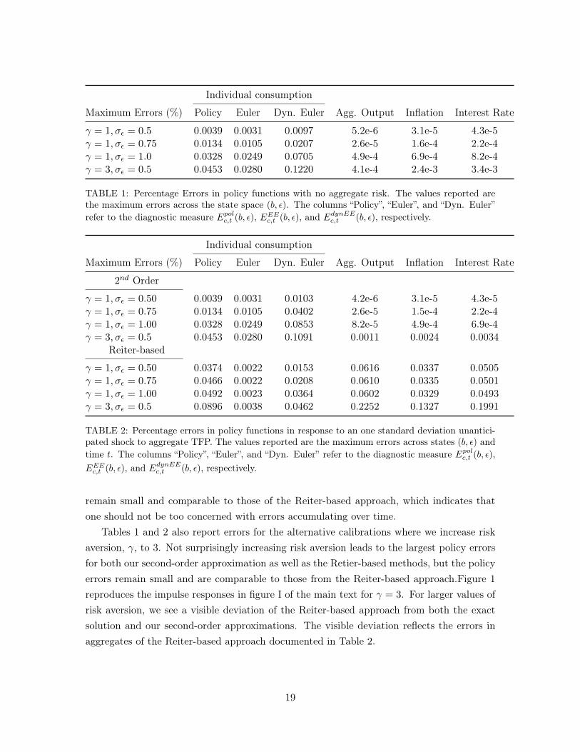
Individual consumption

Maximum Errors (%) Policy Euler Dyn. Euler Agg. Output Inflation Interest Rate

γ = 1, σε = 0.5 0.0039 0.0031 0.0097 5.2e-6 3.1e-5 4.3e-5γ = 1, σε = 0.75 0.0134 0.0105 0.0207 2.6e-5 1.6e-4 2.2e-4γ = 1, σε = 1.0 0.0328 0.0249 0.0705 4.9e-4 6.9e-4 8.2e-4γ = 3, σε = 0.5 0.0453 0.0280 0.1220 4.1e-4 2.4e-3 3.4e-3

TABLE 1: Percentage Errors in policy functions with no aggregate risk. The values reported arethe maximum errors across the state space (b, ε). The columns “Policy”, “Euler”, and “Dyn. Euler”refer to the diagnostic measure Epolc,t (b, ε), EEEc,t (b, ε), and EdynEEc,t (b, ε), respectively.

Individual consumption

Maximum Errors (%) Policy Euler Dyn. Euler Agg. Output Inflation Interest Rate

2nd Order

γ = 1, σε = 0.50 0.0039 0.0031 0.0103 4.2e-6 3.1e-5 4.3e-5γ = 1, σε = 0.75 0.0134 0.0105 0.0402 2.6e-5 1.5e-4 2.2e-4γ = 1, σε = 1.00 0.0328 0.0249 0.0853 8.2e-5 4.9e-4 6.9e-4γ = 3, σε = 0.5 0.0453 0.0280 0.1091 0.0011 0.0024 0.0034

Reiter-based

γ = 1, σε = 0.50 0.0374 0.0022 0.0153 0.0616 0.0337 0.0505γ = 1, σε = 0.75 0.0466 0.0022 0.0208 0.0610 0.0335 0.0501γ = 1, σε = 1.00 0.0492 0.0023 0.0364 0.0602 0.0329 0.0493γ = 3, σε = 0.5 0.0896 0.0038 0.0462 0.2252 0.1327 0.1991

TABLE 2: Percentage errors in policy functions in response to an one standard deviation unantici-pated shock to aggregate TFP. The values reported are the maximum errors across states (b, ε) andtime t. The columns “Policy”, “Euler”, and “Dyn. Euler” refer to the diagnostic measure Epolc,t (b, ε),EEEc,t (b, ε), and EdynEEc,t (b, ε), respectively.

remain small and comparable to those of the Reiter-based approach, which indicates thatone should not be too concerned with errors accumulating over time.

Tables 1 and 2 also report errors for the alternative calibrations where we increase riskaversion, γ, to 3. Not surprisingly increasing risk aversion leads to the largest policy errorsfor both our second-order approximation as well as the Retier-based methods, but the policyerrors remain small and are comparable to those from the Reiter-based approach.Figure 1reproduces the impulse responses in figure I of the main text for γ = 3. For larger values ofrisk aversion, we see a visible deviation of the Reiter-based approach from both the exactsolution and our second-order approximations. The visible deviation reflects the errors inaggregates of the Reiter-based approach documented in Table 2.

19

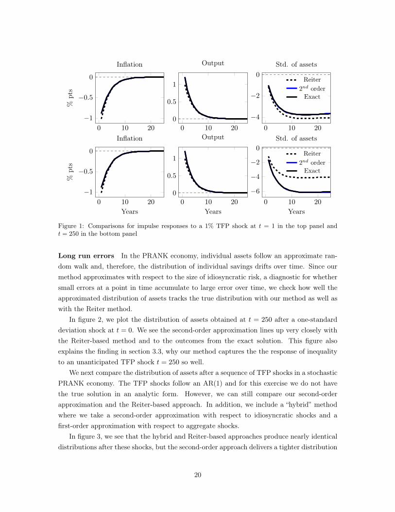
0 10 20

−1

−0.5

0%

pts

Inflation

0 10 20

0

0.5

1

Output

0 10 20

−4

−2

0

Std. of assets

Reiter2nd orderExact

0 10 20

−1

−0.5

0

Years

%pts

Inflation

0 10 20

0

0.5

1

Years

Output

0 10 20

−6

−4

−2

0

Years

Std. of assets

Reiter2nd orderExact

Figure 1: Comparisons for impulse responses to a 1% TFP shock at t = 1 in the top panel andt = 250 in the bottom panel

Long run errors In the PRANK economy, individual assets follow an approximate ran-dom walk and, therefore, the distribution of individual savings drifts over time. Since ourmethod approximates with respect to the size of idiosyncratic risk, a diagnostic for whethersmall errors at a point in time accumulate to large error over time, we check how well theapproximated distribution of assets tracks the true distribution with our method as well aswith the Reiter method.

In figure 2, we plot the distribution of assets obtained at t = 250 after a one-standarddeviation shock at t = 0. We see the second-order approximation lines up very closely withthe Reiter-based method and to the outcomes from the exact solution. This figure alsoexplains the finding in section 3.3, why our method captures the the response of inequalityto an unanticipated TFP shock t = 250 so well.

We next compare the distribution of assets after a sequence of TFP shocks in a stochasticPRANK economy. The TFP shocks follow an AR(1) and for this exercise we do not havethe true solution in an analytic form. However, we can still compare our second-orderapproximation and the Reiter-based approach. In addition, we include a “hybrid” methodwhere we take a second-order approximation with respect to idiosyncratic shocks and afirst-order approximation with respect to aggregate shocks.

In figure 3, we see that the hybrid and Reiter-based approaches produce nearly identicaldistributions after these shocks, but the second-order approach delivers a tighter distribution

20

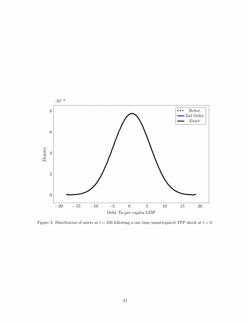
−20 −15 −10 −5 0 5 10 15 20

0

2

4

6

8

·10−2

Debt To per capita GDP

Den

sity

Reiter2nd OrderExact

Figure 2: Distribution of assets at t = 250 following a one time unanticipated TFP shock at t = 0.

21

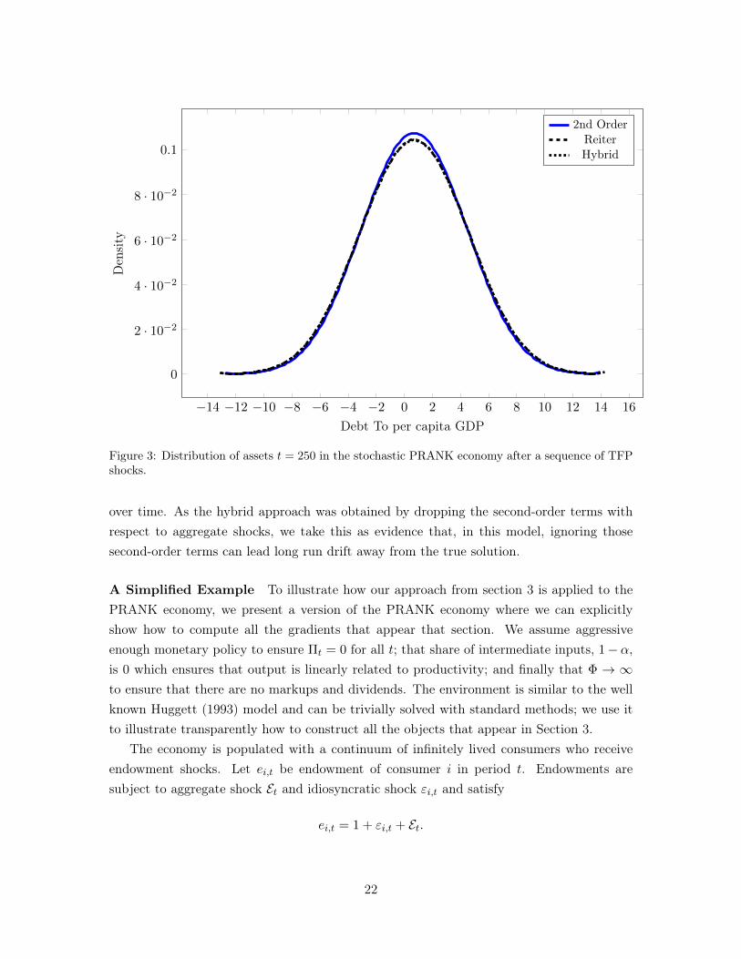
−14 −12 −10 −8 −6 −4 −2 0 2 4 6 8 10 12 14 16

0

2 · 10−2

4 · 10−2

6 · 10−2

8 · 10−2

0.1

Debt To per capita GDP

Den

sity

2nd OrderReiterHybrid

Figure 3: Distribution of assets t = 250 in the stochastic PRANK economy after a sequence of TFPshocks.

over time. As the hybrid approach was obtained by dropping the second-order terms withrespect to aggregate shocks, we take this as evidence that, in this model, ignoring thosesecond-order terms can lead long run drift away from the true solution.

A Simplified Example To illustrate how our approach from section 3 is applied to thePRANK economy, we present a version of the PRANK economy where we can explicitlyshow how to compute all the gradients that appear that section. We assume aggressiveenough monetary policy to ensure Πt = 0 for all t; that share of intermediate inputs, 1− α,is 0 which ensures that output is linearly related to productivity; and finally that Φ → ∞to ensure that there are no markups and dividends. The environment is similar to the wellknown Huggett (1993) model and can be trivially solved with standard methods; we use itto illustrate transparently how to construct all the objects that appear in Section 3.

The economy is populated with a continuum of infinitely lived consumers who receiveendowment shocks. Let ei,t be endowment of consumer i in period t. Endowments aresubject to aggregate shock Et and idiosyncratic shock εi,t and satisfy

ei,t = 1 + εi,t + Et.

22

Shocks Et and εi,t are mean zero and i.i.d. over time.Competitive equilibrium in this economy is fully characterized by consumer budget con-

straint and the Euler equation

ci,t +Qtbi,t − 1− εi,t − Et − bi,t−1 = 0

Qt exp(−γci,t)− βEi,t exp(−γci,t) = 0

as well as the feasibility ∫ci,tdi− 1− Et = 0.

We now show how to use our approximation techniques in this simple example to findcompetitive equilibrium. To make it similar to our notation in Section 3, let y = exp(−γc)and re-write this problem as

ci,t +Qtbi,t − 1− εi,t − Et − bi,t−1 = 0

Qtyi,t − βEi,tyi,t+1 = 0

yi,t − exp(−γci,t) = 0

The first pair of equations correspond to (22) and define mapping F , the last equationcorresponds to (23) and define R. This problem is recursive in the distribution of agents’assets. In our notation of Section 3 we have z = b and Ω is the distribution of b suchthat

∫bdΩ = 0. Vector x of individual policy functions is given by three policy functions[

b c y]T

, and Q is the only aggregate policy function in vector X. Selection matrix p

is simply[

1 0 0].

It is immediate to verify that without shocks consumption smoothing implies that b (b) =

b for all b, so that Lemma 1 holds and equation (27) become

c (b) + Qb (b)− 1− b = 0

Qy (b)− βy(b (b)

)= 0

y (b)− exp (−γc (b)) = 0

and ∫c (b) dΩ− 1 = 0,

which immediately gives Q = β and c (b) = 1 + (1− β) b, y (b) = exp (−γc (b)). From these

23

we construct mappings Rx =[

1 0 0], RX = 0, RE = −1, and Fx−(b) = 0,

Fx (b) =

Q 1 0

0 0 Q

0 −γ exp (−γc(b)) 1

, Fx+ (b) =

0 0 0

0 0 −β0 0 0

, FX (b) =

b

y (b)

0

,

Fε (b) =

−1

0

0

, FE (b) =

−1

0

0

, Fz(z) =

−1

0

0

.All elements of these matrices are know from the zeroth order expansion. Using them, weconstruct first order approximations of policy functions as described in the text.

B Additional details for section 4

In this section we provide details of how we calibrate the initial distribution of nominal andreal claims using the Doepke and Schneider (2006) procedure. Then we show the dynamicsof the calibrated competitive equilibrium using simulations.

Initial distribution of nominal and real claims We combine the rich house-level dataon financial assets from the Survey of Consumer Finances (SCF) and the aggregated Flowof Funds for intermediate investors to obtain nominal and real exposures. We start withthe 2007 Wave of the SCF and restrict our sample to married households who work atleast 100 hours. We drop observations where equity or bond holdings are more than 100times the average yearly wage. These turned out to be about 0.5% of the total sample. Weextract household-level data on their financial holdings and categorize them into (i) deposits,government bonds, liquid assets (net of unsecured credit), (ii) direct holdings of claims tocorporate equities and corporate bonds, and (iii) indirect holdings of (i) and (ii) throughmutual funds and retirement accounts.

We then use Flow of Funds data to obtain balance sheet information for private pensions(Table L.118), for state and local pensions (Table L.119) and mutual funds (Table L.122).Since pension funds have a nontrivial exposure to mutual funds and not vice versa, westart with the aggregated mutual fund balance sheet and map it into broad categories thatrepresent deposits, corporate bonds, government bonds, corporate equities. In the year 2007,mutual funds invested 84 percent of their assets in corporate equities and bonds, 16 percentin government bonds, and other liquid claims.

We next turn pension funds and after aggregating private and public pension funds cate-gorize the combined assets into deposits, government-issued debt, corporate debt, corporate

24

equities, and mutual funds. For the year 2007, the pension funds assets were invested 22percent in mutual funds, 63 percent in corporate equities and bonds, and rest 15 percent ingovernment bonds and other liquid claims.

We define nominal claims as money-like assets plus government issued bonds and claimsto real profits as corporate bonds plus corporate equities. Using the information above, wefirst consolidate the mutual funds into these two categories and then reassign the mutualfunds to pension funds, and finally the mutual funds and pensions funds to the individualsin the SCF.

To fit initial states, we sample directly from the SCF log wages, nominal claims, andclaims to real profits that we constructed. The SCF provides population weights for eachobservation. Given these weights, we set the initial condition by drawing with replacementa random sample of 100000 agents from a discrete distribution.

Properties of the competitive equilibrium In this section, we report several momentsfrom our calibrated competitive equilibrium along a transition path. We draw a sequenceof markup and TFP shocks of length 100 and simulate the competitive equilibrium policiesusing 100000 agents. When we simulate the competitive equilibria, we keep the tax ratesΥt = Υ and use a Taylor rule with Q−1

t = 1βΠ2.5

t .In figure 4, we plot the time series for aggregate output and labor share. We see that

the aggregates are quite stationary and exhibit small fluctuations due to productivity andmarkup shocks. In the table 3 we report cross-sectional moments at dates t ∈ 10, 25, 50, 75.Here we notice a small drift in the distribution of the risk-free assets. The more significantdrifts are in the correlations of of log wages and dividend shares as well as risk-free assetsand dividend shares which steadily declines over time and the correlation between bondsand log wages that increase over time. These patterns are the outcomes of the features inthe baseline that claims to equity are not traded and households are subject to natural debtlimits.

C Additional details for section 5

In the main body, we focused on the results under the baseline calibration and briefly discusssensitivity checks and special cases. In this section, we provide all the omitted details.

C.1 Sensitivity with respect to price adjustment costs

In this section, we present the impulse responses under alternative choices for the priceadjustment cost parameter ψ. As mentioned in section 5.1.1, we vary ψ from twice thebaseline calibration to half of the baseline calibration, and also when ψ is approximately

25

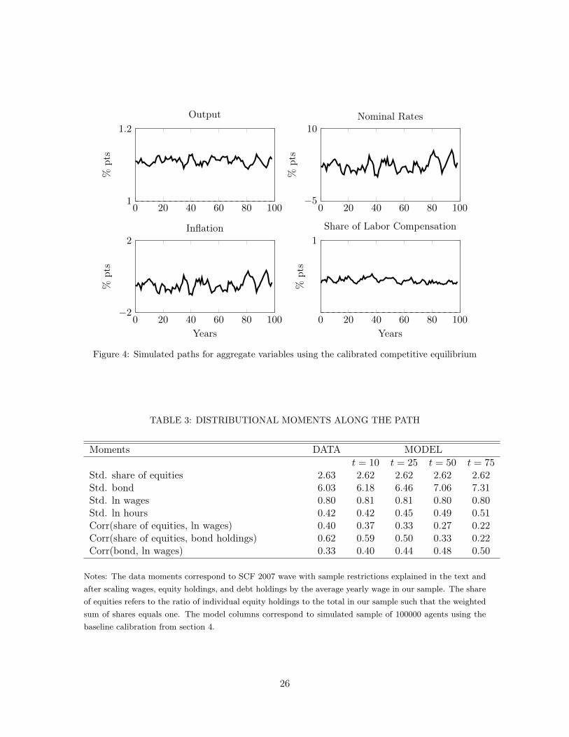
0 20 40 60 80 1001

1.2

%pts

Output

0 20 40 60 80 100−5

10

%pts

Nominal Rates

0 20 40 60 80 100−2

2

Years

%pts

Inflation

0 20 40 60 80 100

1

Years

%pts

Share of Labor Compensation

Figure 4: Simulated paths for aggregate variables using the calibrated competitive equilibrium

TABLE 3: DISTRIBUTIONAL MOMENTS ALONG THE PATH

Moments DATA MODELt = 10 t = 25 t = 50 t = 75

Std. share of equities 2.63 2.62 2.62 2.62 2.62Std. bond 6.03 6.18 6.46 7.06 7.31Std. ln wages 0.80 0.81 0.81 0.80 0.80Std. ln hours 0.42 0.42 0.45 0.49 0.51Corr(share of equities, ln wages) 0.40 0.37 0.33 0.27 0.22Corr(share of equities, bond holdings) 0.62 0.59 0.50 0.33 0.22Corr(bond, ln wages) 0.33 0.40 0.44 0.48 0.50

Notes: The data moments correspond to SCF 2007 wave with sample restrictions explained in the text andafter scaling wages, equity holdings, and debt holdings by the average yearly wage in our sample. The shareof equities refers to the ratio of individual equity holdings to the total in our sample such that the weightedsum of shares equals one. The model columns correspond to simulated sample of 100000 agents using thebaseline calibration from section 4.

26

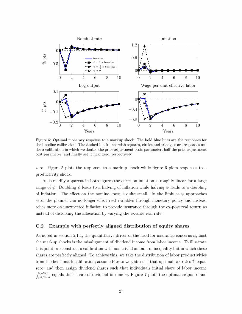
0 2 4 6 8 10

0

−0.5%pts

Nominal rate

baseline

ψ = 2× baseline

ψ = 12× baseline

ψ ≈ 0

0 2 4 6 8 10

0

0.6

1.2

Inflation

0 2 4 6 8 10−0.2

−0.1

0

0.1

Years

%pts

Log output

0 2 4 6 8 10

−0.8

−0.4

0

Years

Wage per unit effective labor

Figure 5: Optimal monetary response to a markup shock. The bold blue lines are the responses forthe baseline calibration. The dashed black lines with squares, circles and triangles are responses un-der a calibration in which we double the price adjustment costs parameter, half the price adjustmentcost parameter, and finally set it near zero, respectively.

zero. Figure 5 plots the responses to a markup shock while figure 6 plots responses to aproductivity shock.

As is readily apparent in both figures the effect on inflation is roughly linear for a largerange of ψ. Doubling ψ leads to a halving of inflation while halving ψ leads to a doublingof inflation. The effect on the nominal rate is quite small. In the limit as ψ approacheszero, the planner can no longer effect real variables through monetary policy and insteadrelies more on unexpected inflation to provide insurance through the ex-post real return asinstead of distorting the allocation by varying the ex-ante real rate.

C.2 Example with perfectly aligned distribution of equity shares

As noted in section 5.1.1, the quantitative driver of the need for insurance concerns againstthe markup shocks is the misalignment of dividend income from labor income. To illustratethis point, we construct a calibration with non trivial amount of inequality but in which theseshares are perfectly aligned. To achieve this, we take the distribution of labor productivitiesfrom the benchmark calibration; assume Pareto weights such that optimal tax rates Υ equalzero; and then assign dividend shares such that individuals initial share of labor incomeεi,oni,0∫i εi,0ni,0

equals their share of dividend income si. Figure 7 plots the optimal response and

27

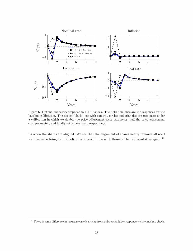
0 2 4 6 8 10

1

0

−1

%pts

Nominal rate

baseline

ψ = 2× baseline

ψ = 12× baseline

ψ ≈ 0

0 2 4 6 8 10

0

1

2

Inflation

0 2 4 6 8 10−0.8

−0.4

0

Years

%pts

Log output

0 2 4 6 8 10

−2

−1

0

1

Years

Real rate

Figure 6: Optimal monetary response to a TFP shock. The bold blue lines are the responses for thebaseline calibration. The dashed black lines with squares, circles and triangles are responses undera calibration in which we double the price adjustment costs parameter, half the price adjustmentcost parameter, and finally set it near zero, respectively.

its when the shares are aligned. We see that the alignment of shares nearly removes all needfor insurance bringing the policy responses in line with those of the representative agent.41

41There is some difference in insurance needs arising from differential labor responses to the markup shock.

28

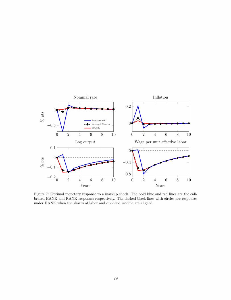
0 2 4 6 8 10

0

−0.5

%pts

Nominal rate

Benchmark

Aligned Shares

RANK

0 2 4 6 8 10

0

0.2

Inflation

0 2 4 6 8 10−0.2

−0.1

0

0.1

Years

%pts

Log output

0 2 4 6 8 10

−0.8

−0.4

0

Years

Wage per unit effective labor

Figure 7: Optimal monetary response to a markup shock. The bold blue and red lines are the cali-brated HANK and RANK responses respectively. The dashed black lines with circles are responsesunder HANK when the shares of labor and dividend income are aligned.

29

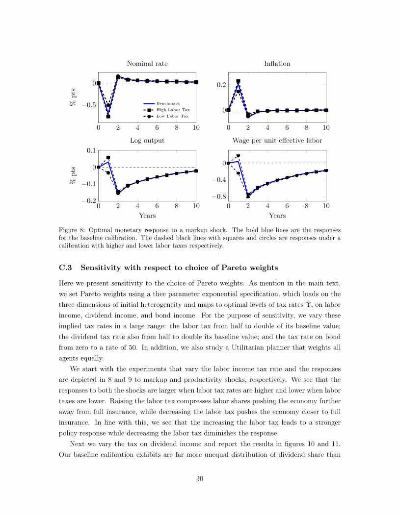
0 2 4 6 8 10

0

−0.5%pts

Nominal rate

Benchmark

High Labor Tax

Low Labor Tax

0 2 4 6 8 10

0

0.2

Inflation

0 2 4 6 8 10−0.2

−0.1

0

0.1

Years

%pts

Log output

0 2 4 6 8 10

−0.8

−0.4

0

Years

Wage per unit effective labor

Figure 8: Optimal monetary response to a markup shock. The bold blue lines are the responsesfor the baseline calibration. The dashed black lines with squares and circles are responses under acalibration with higher and lower labor taxes respectively.

C.3 Sensitivity with respect to choice of Pareto weights

Here we present sensitivity to the choice of Pareto weights. As mention in the main text,we set Pareto weights using a thee parameter exponential specification, which loads on thethree dimensions of initial heterogeneity and maps to optimal levels of tax rates Υ, on laborincome, dividend income, and bond income. For the purpose of sensitivity, we vary theseimplied tax rates in a large range: the labor tax from half to double of its baseline value;the dividend tax rate also from half to double its baseline value; and the tax rate on bondfrom zero to a rate of 50. In addition, we also study a Utilitarian planner that weights allagents equally.

We start with the experiments that vary the labor income tax rate and the responsesare depicted in 8 and 9 to markup and productivity shocks, respectively. We see that theresponses to both the shocks are larger when labor tax rates are higher and lower when labortaxes are lower. Raising the labor tax compresses labor shares pushing the economy furtheraway from full insurance, while decreasing the labor tax pushes the economy closer to fullinsurance. In line with this, we see that the increasing the labor tax leads to a strongerpolicy response while decreasing the labor tax diminishes the response.

Next we vary the tax on dividend income and report the results in figures 10 and 11.Our baseline calibration exhibits are far more unequal distribution of dividend share than

30

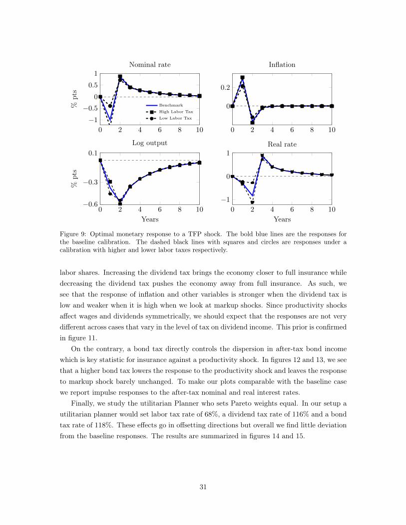
0 2 4 6 8 10

1

0.5

0

−0.5

−1

%pts

Nominal rate

Benchmark

High Labor Tax

Low Labor Tax

0 2 4 6 8 10

0

0.2

Inflation

0 2 4 6 8 10−0.6

−0.3

0.1

Years

%pts

Log output

0 2 4 6 8 10

−1

0

1

Years

Real rate

Figure 9: Optimal monetary response to a TFP shock. The bold blue lines are the responses forthe baseline calibration. The dashed black lines with squares and circles are responses under acalibration with higher and lower labor taxes respectively.

labor shares. Increasing the dividend tax brings the economy closer to full insurance whiledecreasing the dividend tax pushes the economy away from full insurance. As such, wesee that the response of inflation and other variables is stronger when the dividend tax islow and weaker when it is high when we look at markup shocks. Since productivity shocksaffect wages and dividends symmetrically, we should expect that the responses are not verydifferent across cases that vary in the level of tax on dividend income. This prior is confirmedin figure 11.

On the contrary, a bond tax directly controls the dispersion in after-tax bond incomewhich is key statistic for insurance against a productivity shock. In figures 12 and 13, we seethat a higher bond tax lowers the response to the productivity shock and leaves the responseto markup shock barely unchanged. To make our plots comparable with the baseline casewe report impulse responses to the after-tax nominal and real interest rates.

Finally, we study the utilitarian Planner who sets Pareto weights equal. In our setup autilitarian planner would set labor tax rate of 68%, a dividend tax rate of 116% and a bondtax rate of 118%. These effects go in offsetting directions but overall we find little deviationfrom the baseline responses. The results are summarized in figures 14 and 15.

31

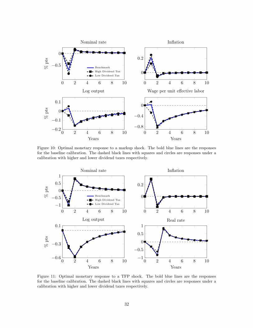
0 2 4 6 8 10

0

−0.5

%pts

Nominal rate

Benchmark

High Dividend Tax

Low Dividend Tax

0 2 4 6 8 10

0

0.2

Inflation

0 2 4 6 8 10−0.2

−0.1

0

0.1

Years

%pts

Log output

0 2 4 6 8 10

−0.8

−0.4

0

Years

Wage per unit effective labor

Figure 10: Optimal monetary response to a markup shock. The bold blue lines are the responsesfor the baseline calibration. The dashed black lines with squares and circles are responses under acalibration with higher and lower dividend taxes respectively.

0 2 4 6 8 10

1

0.5

0

−0.5

−1

%pts

Nominal rate

Benchmark

High Dividend Tax

Low Dividend Tax

0 2 4 6 8 10

0

0.2

Inflation

0 2 4 6 8 10−0.6

−0.3

0.1

Years

%pts

Log output

0 2 4 6 8 10−1

−0.5

0

0.5

1

Years

Real rate

Figure 11: Optimal monetary response to a TFP shock. The bold blue lines are the responsesfor the baseline calibration. The dashed black lines with squares and circles are responses under acalibration with higher and lower dividend taxes respectively.

32

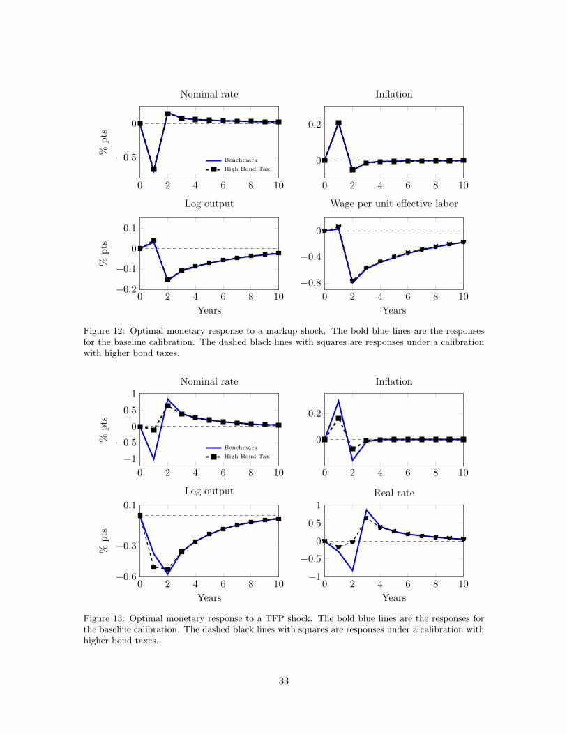
0 2 4 6 8 10

0

−0.5

%pts

Nominal rate

Benchmark

High Bond Tax

0 2 4 6 8 10

0

0.2

Inflation

0 2 4 6 8 10−0.2

−0.1

0

0.1

Years

%pts

Log output

0 2 4 6 8 10

−0.8

−0.4

0

Years

Wage per unit effective labor

Figure 12: Optimal monetary response to a markup shock. The bold blue lines are the responsesfor the baseline calibration. The dashed black lines with squares are responses under a calibrationwith higher bond taxes.

0 2 4 6 8 10

1

0.5

0

−0.5

−1

%pts

Nominal rate

Benchmark

High Bond Tax

0 2 4 6 8 10

0

0.2

Inflation

0 2 4 6 8 10−0.6

−0.3

0.1

Years

%pts

Log output

0 2 4 6 8 10−1

−0.5

0

0.5

1

Years

Real rate

Figure 13: Optimal monetary response to a TFP shock. The bold blue lines are the responses forthe baseline calibration. The dashed black lines with squares are responses under a calibration withhigher bond taxes.

33

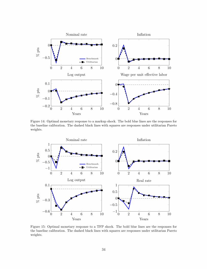
0 2 4 6 8 10

0

−0.5

%pts

Nominal rate

Benchmark

Utilitarian

0 2 4 6 8 10

0

0.2

Inflation

0 2 4 6 8 10−0.2

−0.1

0

0.1

Years

%pts

Log output

0 2 4 6 8 10

−0.8

−0.4

0

Years

Wage per unit effective labor

Figure 14: Optimal monetary response to a markup shock. The bold blue lines are the responses forthe baseline calibration. The dashed black lines with squares are responses under utilitarian Paretoweights.

0 2 4 6 8 10

1

0.5

0

−0.5

−1

%pts

Nominal rate

Benchmark

Utilitarian

0 2 4 6 8 10

0

0.2

Inflation

0 2 4 6 8 10−0.6

−0.3

0.1

Years

%pts

Log output

0 2 4 6 8 10−1

−0.5

0

0.5

1

Years

Real rate

Figure 15: Optimal monetary response to a TFP shock. The bold blue lines are the responses forthe baseline calibration. The dashed black lines with squares are responses under utilitarian Paretoweights.

34

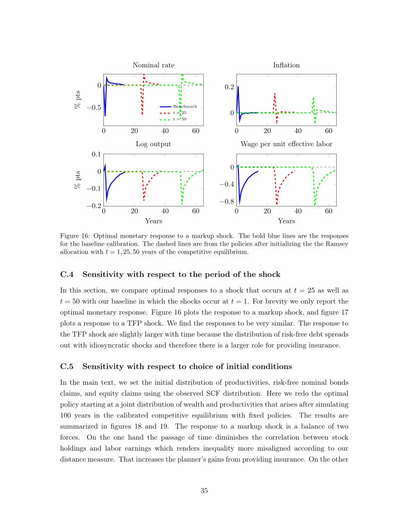
0 20 40 60

0

−0.5%pts

Nominal rate

Benchmark

t = 25

t = 50

0 20 40 60

0

0.2

Inflation

0 20 40 60−0.2

−0.1

0

0.1

Years

%pts

Log output

0 20 40 60

−0.8

−0.4

0

Years

Wage per unit effective labor

Figure 16: Optimal monetary response to a markup shock. The bold blue lines are the responsesfor the baseline calibration. The dashed lines are from the policies after initializing the the Ramseyallocation with t = 1, 25, 50 years of the competitive equilibrium.

C.4 Sensitivity with respect to the period of the shock

In this section, we compare optimal responses to a shock that occurs at t = 25 as well ast = 50 with our baseline in which the shocks occur at t = 1. For brevity we only report theoptimal monetary response. Figure 16 plots the response to a markup shock, and figure 17plots a response to a TFP shock. We find the responses to be very similar. The response tothe TFP shock are slightly larger with time because the distribution of risk-free debt spreadsout with idiosyncratic shocks and therefore there is a larger role for providing insurance.

C.5 Sensitivity with respect to choice of initial conditions

In the main text, we set the initial distribution of productivities, risk-free nominal bondsclaims, and equity claims using the observed SCF distribution. Here we redo the optimalpolicy starting at a joint distribution of wealth and productivities that arises after simulating100 years in the calibrated competitive equilibrium with fixed policies. The results aresummarized in figures 18 and 19. The response to a markup shock is a balance of twoforces. On the one hand the passage of time diminishes the correlation between stockholdings and labor earnings which renders inequality more misaligned according to ourdistance measure. That increases the planner’s gains from providing insurance. On the other

35

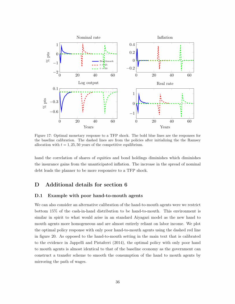
0 20 40 60

1

0

−1

−2

%pts

Nominal rate

Benchmark

t = 25

t = 50

0 20 40 60

−0.2

0

0.2

0.4

Inflation

0 20 40 60

−0.6

−0.3

0.1

Years

%pts

Log output

0 20 40 60

−1

0

1

Years

Real rate

Figure 17: Optimal monetary response to a TFP shock. The bold blue lines are the responses forthe baseline calibration. The dashed lines are from the policies after initializing the the Ramseyallocation with t = 1, 25, 50 years of the competitive equilibrium.

hand the correlation of shares of equities and bond holdings diminishes which diminishesthe insurance gains from the unanticipated inflation. The increase in the spread of nominaldebt leads the planner to be more responsive to a TFP shock.

D Additional details for section 6

D.1 Example with poor hand-to-mouth agents

We can also consider an alternative calibration of the hand-to-mouth agents were we restrictbottom 15% of the cash-in-hand distribution to be hand-to-mouth. This environment issimilar in spirit to what would arise in an standard Aiyagari model as the new hand tomouth agents more homogeneous and are almost entirely reliant on labor income. We plotthe optimal policy response with only poor hand-to-mouth agents using the dashed red linein figure 20. As opposed to the hand-to-mouth setting in the main text that is calibratedto the evidence in Jappelli and Pistaferri (2014), the optimal policy with only poor handto mouth agents is almost identical to that of the baseline economy as the government canconstruct a transfer scheme to smooth the consumption of the hand to mouth agents bymirroring the path of wages.

36

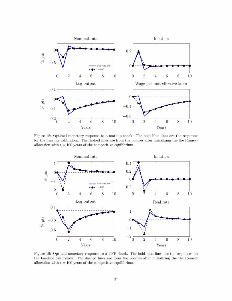
0 2 4 6 8 10

0

−0.5%pts

Nominal rate

Benchmark

t=100

0 2 4 6 8 10

0

0.2

Inflation

0 2 4 6 8 10−0.2

−0.1

0

0.1

Years

%pts

Log output

0 2 4 6 8 10

−0.8

−0.4

0

Years

Wage per unit effective labor

Figure 18: Optimal monetary response to a markup shock. The bold blue lines are the responsesfor the baseline calibration. The dashed lines are from the policies after initializing the the Ramseyallocation with t = 100 years of the competitive equilibrium.

0 2 4 6 8 10

1

0

−1

−2

%pts

Nominal rate

Benchmark

t=100

0 2 4 6 8 10

−0.2

0

0.2

0.4

Inflation

0 2 4 6 8 10

−0.6

−0.3

0.1

Years

%pts

Log output

0 2 4 6 8 10−2

−1

0

1

Years

Real rate

Figure 19: Optimal monetary response to a TFP shock. The bold blue lines are the responses forthe baseline calibration. The dashed lines are from the policies after initializing the the Ramseyallocation with t = 100 years of the competitive equilibrium.

37

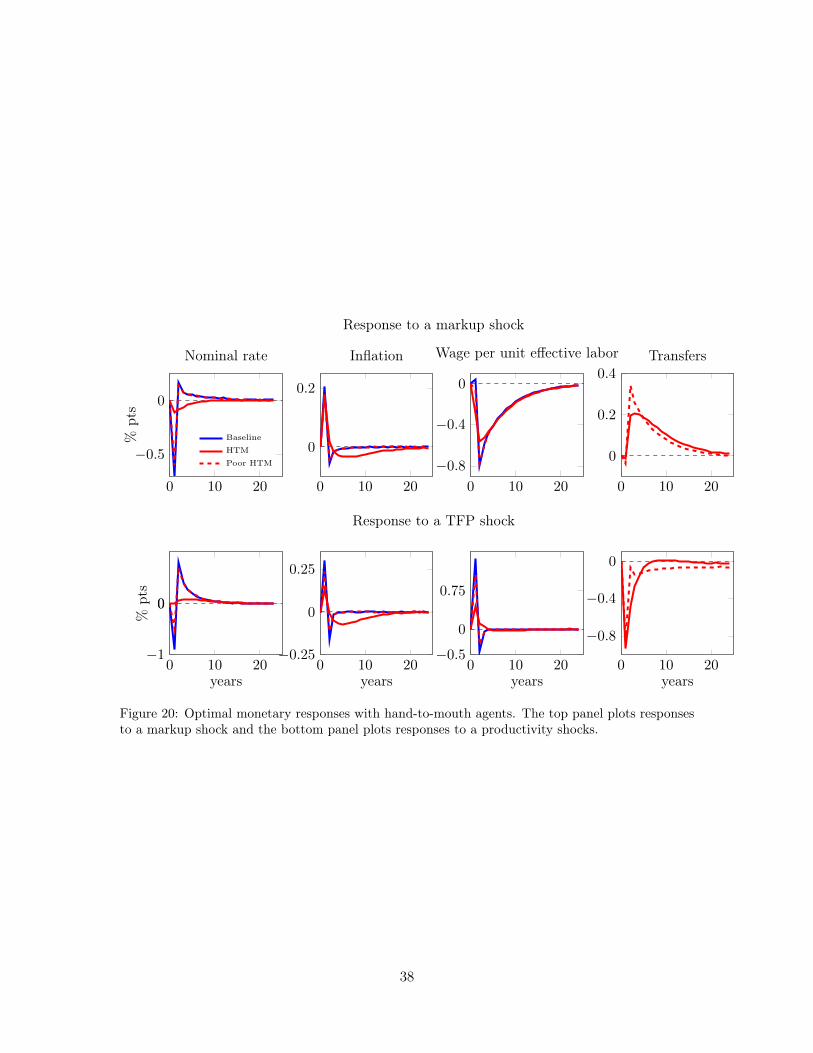
Response to a markup shock

Response to a TFP shock

0 10 20

0

−0.5

%pts

Nominal rate

Baseline

HTM

Poor HTM

0 10 20

0

0.2

Inflation

0 10 20

−0.8

−0.4

0

Wage per unit effective labor

0 10 20

0

0.2

0.4Transfers

0 10 20−1

00

years

%pts

0 10 20−0.25

0

0.25

years0 10 20

−0.5

0

0.75

years0 10 20

−0.8

−0.4

0

years

Figure 20: Optimal monetary responses with hand-to-mouth agents. The top panel plots responsesto a markup shock and the bottom panel plots responses to a productivity shocks.

38

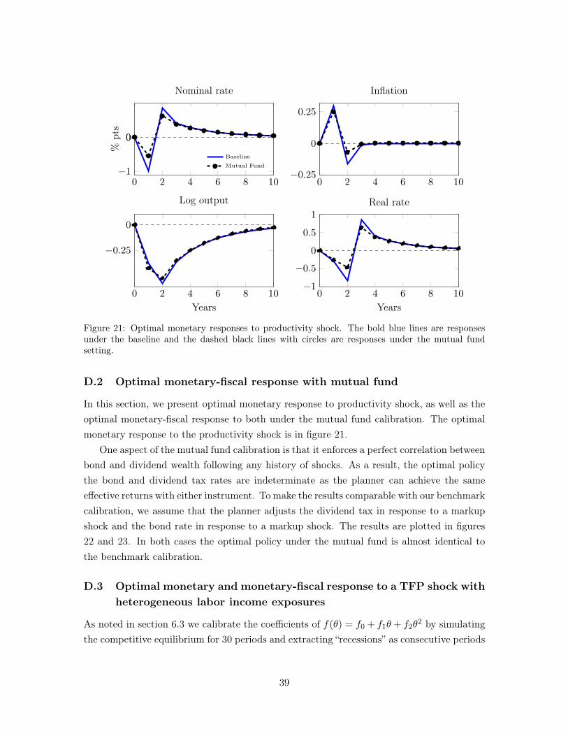
0 2 4 6 8 10−1

00

%pts

Nominal rate

Baseline

Mutual Fund

0 2 4 6 8 10−0.25

0

0.25

Inflation

0 2 4 6 8 10

−0.25

0

Years

Log output

0 2 4 6 8 10−1

−0.5

0

0.5

1

Years

Real rate

Figure 21: Optimal monetary responses to productivity shock. The bold blue lines are responsesunder the baseline and the dashed black lines with circles are responses under the mutual fundsetting.

D.2 Optimal monetary-fiscal response with mutual fund

In this section, we present optimal monetary response to productivity shock, as well as theoptimal monetary-fiscal response to both under the mutual fund calibration. The optimalmonetary response to the productivity shock is in figure 21.

One aspect of the mutual fund calibration is that it enforces a perfect correlation betweenbond and dividend wealth following any history of shocks. As a result, the optimal policythe bond and dividend tax rates are indeterminate as the planner can achieve the sameeffective returns with either instrument. To make the results comparable with our benchmarkcalibration, we assume that the planner adjusts the dividend tax in response to a markupshock and the bond rate in response to a markup shock. The results are plotted in figures22 and 23. In both cases the optimal policy under the mutual fund is almost identical tothe benchmark calibration.

D.3 Optimal monetary and monetary-fiscal response to a TFP shock withheterogeneous labor income exposures

As noted in section 6.3 we calibrate the coefficients of f(θ) = f0 + f1θ+ f2θ2 by simulating

the competitive equilibrium for 30 periods and extracting “recessions” as consecutive periods

39

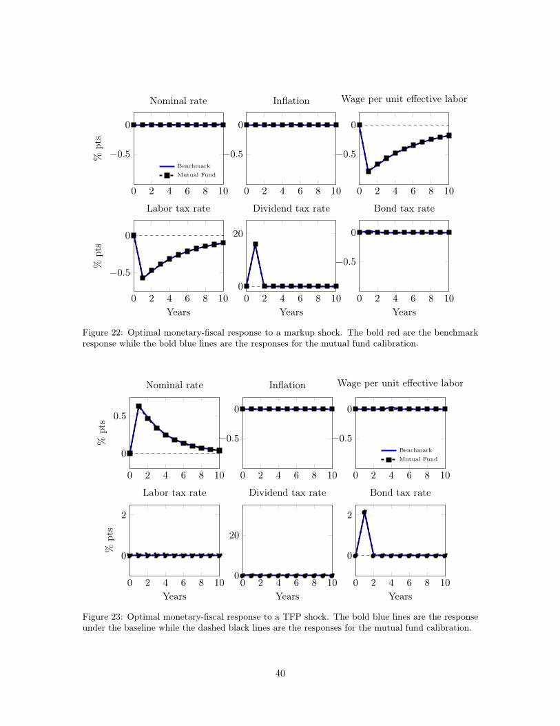
0 2 4 6 8 10

−0.5

0

%pts

Nominal rate

Benchmark

Mutual Fund

0 2 4 6 8 10

−0.5

0

Inflation

0 2 4 6 8 10

−0.5

0

Wage per unit effective labor

0 2 4 6 8 10

−0.5

0

Years

%pts

Labor tax rate

0 2 4 6 8 100

20

Years

Dividend tax rate

0 2 4 6 8 10

−0.5

0

Years

Bond tax rate

Figure 22: Optimal monetary-fiscal response to a markup shock. The bold red are the benchmarkresponse while the bold blue lines are the responses for the mutual fund calibration.

0 2 4 6 8 10

0

0.5

%pts

Nominal rate

0 2 4 6 8 10

−0.5

0

Inflation

0 2 4 6 8 10

−0.5

0

Wage per unit effective labor

Benchmark

Mutual Fund

0 2 4 6 8 10

0

2

Years

%pts

Labor tax rate

0 2 4 6 8 100

20

Years

Dividend tax rate

0 2 4 6 8 10

0

2

Years

Bond tax rate

Figure 23: Optimal monetary-fiscal response to a TFP shock. The bold blue lines are the responseunder the baseline while the dashed black lines are the responses for the mutual fund calibration.

40

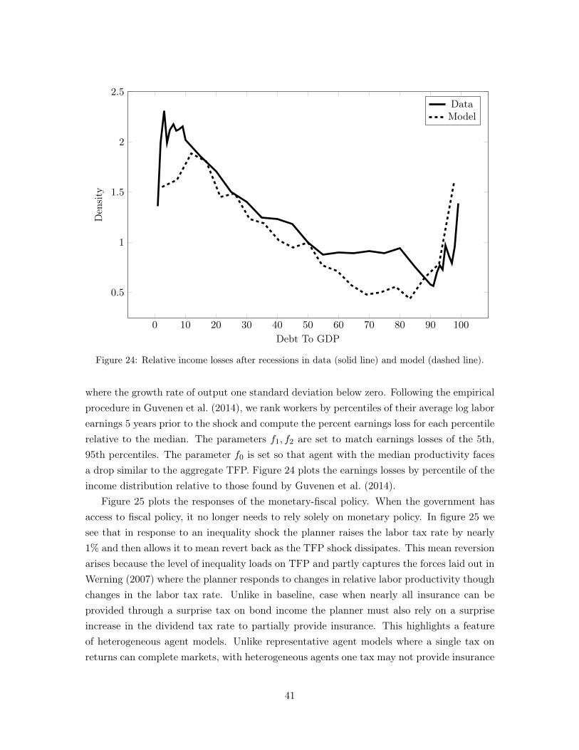
0 10 20 30 40 50 60 70 80 90 100

0.5

1

1.5

2

2.5

Debt To GDP

Den

sity

DataModel

Figure 24: Relative income losses after recessions in data (solid line) and model (dashed line).

where the growth rate of output one standard deviation below zero. Following the empiricalprocedure in Guvenen et al. (2014), we rank workers by percentiles of their average log laborearnings 5 years prior to the shock and compute the percent earnings loss for each percentilerelative to the median. The parameters f1, f2 are set to match earnings losses of the 5th,95th percentiles. The parameter f0 is set so that agent with the median productivity facesa drop similar to the aggregate TFP. Figure 24 plots the earnings losses by percentile of theincome distribution relative to those found by Guvenen et al. (2014).

Figure 25 plots the responses of the monetary-fiscal policy. When the government hasaccess to fiscal policy, it no longer needs to rely solely on monetary policy. In figure 25 wesee that in response to an inequality shock the planner raises the labor tax rate by nearly1% and then allows it to mean revert back as the TFP shock dissipates. This mean reversionarises because the level of inequality loads on TFP and partly captures the forces laid out inWerning (2007) where the planner responds to changes in relative labor productivity thoughchanges in the labor tax rate. Unlike in baseline, case when nearly all insurance can beprovided through a surprise tax on bond income the planner must also rely on a surpriseincrease in the dividend tax rate to partially provide insurance. This highlights a featureof heterogeneous agent models. Unlike representative agent models where a single tax onreturns can complete markets, with heterogeneous agents one tax may not provide insurance

41

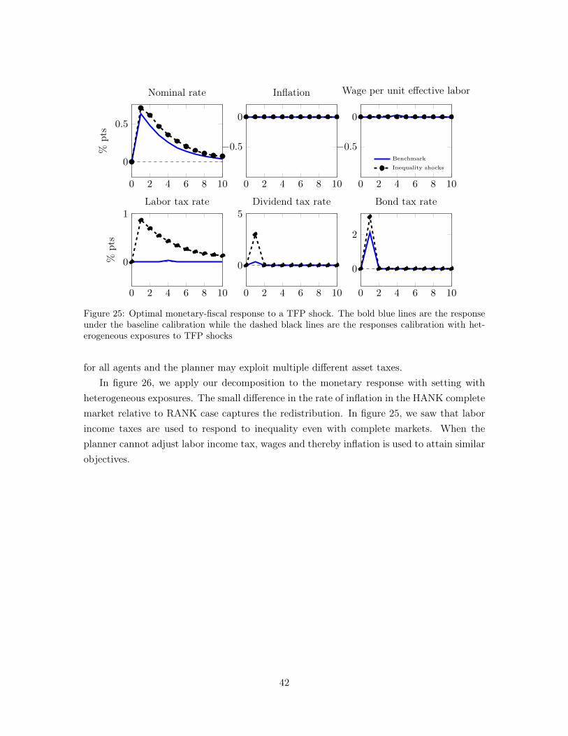
0 2 4 6 8 10

0

0.5

%pts

Nominal rate

0 2 4 6 8 10

−0.5

0

Inflation

0 2 4 6 8 10

−0.5

0

Wage per unit effective labor

Benchmark

Inequality shocks

0 2 4 6 8 10

0

1

%pts

Labor tax rate

0 2 4 6 8 10

0

5Dividend tax rate

0 2 4 6 8 10

0

2

Bond tax rate

Figure 25: Optimal monetary-fiscal response to a TFP shock. The bold blue lines are the responseunder the baseline calibration while the dashed black lines are the responses calibration with het-erogeneous exposures to TFP shocks

for all agents and the planner may exploit multiple different asset taxes.In figure 26, we apply our decomposition to the monetary response with setting with

heterogeneous exposures. The small difference in the rate of inflation in the HANK completemarket relative to RANK case captures the redistribution. In figure 25, we saw that laborincome taxes are used to respond to inequality even with complete markets. When theplanner cannot adjust labor income tax, wages and thereby inflation is used to attain similarobjectives.

42

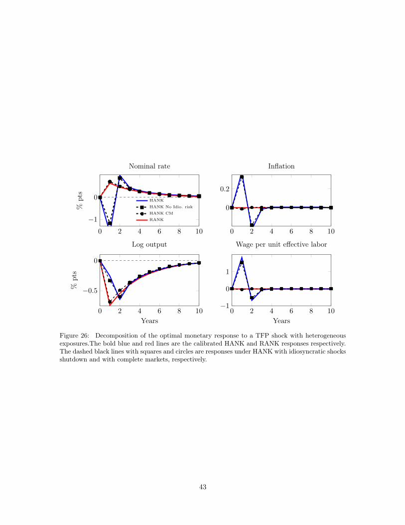
0 2 4 6 8 10

−1

0

%pts

Nominal rate

HANK

HANK No Idio. risk

HANK CM

RANK

0 2 4 6 8 10

0

0.2

Inflation

0 2 4 6 8 10

−0.5

0

Years

%pts

Log output

0 2 4 6 8 10−1

0

1

Years

Wage per unit effective labor

Figure 26: Decomposition of the optimal monetary response to a TFP shock with heterogeneousexposures.The bold blue and red lines are the calibrated HANK and RANK responses respectively.The dashed black lines with squares and circles are responses under HANK with idiosyncratic shocksshutdown and with complete markets, respectively.

43