Benthic oxygen consumption rates during hypoxic conditions ... · oxygen consumption rates during hypoxic conditions on the Oregon continental shelf: Evaluation of the eddy correlation

Benthic oxygen consumption rates during hypoxic conditionson the Oregon continental shelf: Evaluation of the eddycorrelation method

Clare E. Reimers,1 H. Tuba Özkan-Haller,1 Peter Berg,2 Allan Devol,3

Kristina McCann-Grosvenor,1 and Rhea D. Sanders1

Received 1 September 2011; revised 6 December 2011; accepted 11 December 2011; published 10 February 2012.

[1] Three stations, at �80 m water depth on the Oregon shelf between 44.7°N and 43.9 N,were studied under hypoxic conditions in late spring and summer of 2009 to determinebenthic oxygen consumption rates. Oxygen fluxes were derived from eddy correlation (EC)measurements made from an autonomous lander deployed for 11–15 h at a time. Averageoxygen consumption rates ranged from 3.2 to 9.8 mmol m�2 d�1 and were highest atthe southernmost station. Methods for separating eddy components and rotating coordinateswere examined for effects on EC fluxes. It was found that oscillations at frequenciesassociated with surface and internal waves made significant contributions, but horizontalcomponent biasing could be minimized by wave-based rotation methods. Additionalmeasurements included benthic boundary layer properties, and sediment permeability andprofiles of sediment organic C, chlorophyll-a, excess 210Pb and % fines. Comparativeflux estimates were determined from benthic chamber measurements and microelectrodeprofiles at two of the stations. The chamber O2 consumption rates exceeded the EC fluxes byfactors of 1.2–1.8, which may reflect enclosure effects, the different spatial and temporalscales of the measurements, and/or inhomogeneous benthic respiration rates. Themagnitudes of the fluxes by either method, however, are low for shelf depths. Thus, forbenthic O2 consumption to contribute to Oregon shelf hypoxia, bottom waters must beslowly renewed and minimally ventilated by along- or across-shelf advection and turbulentmixing. Circulation studies indicate these conditions are favored by increased near-bottomstratification during persistent summer upwelling- relaxation cycles.

Citation: Reimers, C. E., H. T. Özkan-Haller, P. Berg, A. Devol, K. McCann-Grosvenor, and R. D. Sanders (2012), Benthicoxygen consumption rates during hypoxic conditions on the Oregon continental shelf: Evaluation of the eddy correlation method,J. Geophys. Res., 117, C02021, doi:10.1029/2011JC007564.

1. Introduction

[2] In recent years eddy correlation (EC) has gainedacceptance as a valid technique for determining dissolvedoxygen (O2) fluxes between aquatic sediments and overlyingwater masses. To derive an O2 eddy flux, the covariancebetween high-resolution fluctuations of both O2 and verticalvelocity measured above the sediment surface (typically ata height between 10 and 20 cm) is computed. Among EC’sdescribed advantages are that (1) measurements are madeunder natural light and hydrodynamic conditions, (2) thesediments are not enclosed or disturbed, and (3) derivedfluxes reflect benthic O2 exchange processes occurring over

large sediment surface areas (tens of square meters) [Berget al., 2007]. EC aquatic applications are increasing andinclude studies of O2 dynamics in a shallow river bed, twolakes, a variety of nearshore marine environments, and a deepmarine bay [Berg et al., 2003, 2009; Kuwae et al., 2006;McGinnis et al., 2008; Brand et al., 2008; Berg and Huettel,2008; Glud et al., 2010; Hume et al., 2011]. The method isanalogous to the measurement of near-bottom, turbulence-induced heat and momentum fluxes often undertaken byphysical oceanographers [e.g., Shaw and Trowbridge, 2001].However, it also requires many of the same assumptionsabout conditions, mass balance, and data filtering-correctiontechniques that are used by boundary layer meteorologists todiscriminate between good and erroneous gas flux measure-ments at land-atmosphere interfaces [e.g., Finnigan, 1999;Finnigan et al., 2003; Aubinet, 2008]. Thus, these assump-tions should be reevaluated in every new field situation.[3] In this paper, EC measurements are reported that were

made on the central Oregon continental shelf in late springand summer of 2009 during conditions of coastal upwelling,hypoxia, and moderate wave energy. The acquisition ofEC data in this dynamic and challenging environment was

1College of Oceanic and Atmospheric Sciences, Oregon State University,Corvallis, Oregon, USA.

2Department of Environmental Sciences, University of Virginia,Charlottesville, Virginia, USA.

3School of Oceanography, University of Washington, Seattle, Washington,USA.

Copyright 2012 by the American Geophysical Union.0148-0227/12/2011JC007564

JOURNAL OF GEOPHYSICAL RESEARCH, VOL. 117, C02021, doi:10.1029/2011JC007564, 2012

C02021 1 of 18

http://dx.doi.org/10.1029/2011JC007564

enabled by the development of a unique benthic tripoddeployed in a moored mode and equipped with sensors and arotating digital still camera. Simultaneous pressure data areused to evaluate the influences of the wave-induced velocityfield on EC components. Detrending and coordinate rotationapproaches are compared to adopt “best practices” forderiving O2 eddy fluxes at these study sites and understand-ing what they represent in terms of a desired measure of thetotal benthic O2 consumption rate.[4] The central continental shelf of Oregon is part of a

narrow oceanic eastern boundary current margin [Chen et al.,2004; Jahnke, 2010] where equatorward winds intermittentlydrive offshore surface Ekman transport and the upwelling ofcold, nutrient-rich and O2-depleted water during spring andsummer [Barth et al., 2007; Chan et al., 2008]; in contrast,large wind waves associated with North Pacific storm pat-terns dominate water column mixing during winter [Allan andKomar, 2006]. Spatial and temporal changes in phytoplanktonproduction, the alongshore coastal jet, and a particle-enrichedbenthic boundary layer are expected to have an impact onpatterns of organic matter transport and consequently respi-ration in both the water column and sediments [Castelao andBarth, 2005; Perlin et al., 2005; Hales et al., 2006]. Inshoreof the 100 m isobath, the sediments are predominantly finesand that is subject to resuspension and particulate organicmatter entrapment (filtering) by both physical transport(including oscillatory ripple migration) and bioturbation[Komar et al., 1972; Kulm, 1978]. These properties andprocesses, together with a potential for wave pumping ofbottom water into the bed, complicate assessments of the

benthic role in O2 or coupled carbon budgets [Riedl et al.,1972; Shum and Sundby, 1996; Huettel and Webster,2001]. In fact, no measurements of benthic O2 uptake madeby traditional benthic chamber or microprofiling methodshave been reported for sites <100 m on the Oregon shelf.Devol and Christensen [1993] do report chamber fluxes of�5 to �18 mmol O2 m�2 d�1 from the neighboringWashington shelf, with the highest rates occurring at 114 mwater depth associated with a midshelf silt deposit. Similarly,historic deficits of O2 and nitrate that increase along salinitysurfaces led Connolly et al. [2010] to infer that Washingtonshelf sediments are a regular sink for �1 � 0.2 mM O2 d

�1

from the bottom boundary layer. This depletion rate suggestssediment respiration contributes to episodes of severe shelfhypoxia nearly equally with water column respiration[Connolly et al., 2010].[5] Certainly, an understanding of how ecosystem pro-

cesses respond to local forcing or are linked to ocean basin-scale changes requires trusted baseline measurements. TheEC technique produces rich data sets that yield informationon local waves, currents, turbulence, and their impacts onbenthic O2 fluxes. In this paper we examine EC data from theOregon shelf with a focus on three midshelf stations. Watercolumn, sediment, O2 microprofile, and benthic chamberdata are also used to assess the along-shelf variability oforganic carbon respiration and the comparability of ECoxygen fluxes with estimates from traditional methods.

2. Materials and Methods

2.1. Study Sites

[6] The study sites were occupied during cruises of theR/V Wecoma in June and August 2009. The stations aredesignated NH, SH, and HH for their proximity to theNewport (Oregon) hydrographic line and coastal featuresknown as Strawberry Hill and Hecata Head, respectively[Grantham et al., 2004]. They were located near the 80 misobath in low-relief areas of sandy sediments at approxi-mately 44.65°N, 124.30°W; 44.24°N, 124.32°W; and43.93°N, 124.25°W, respectively (Figure 1).

2.2. BOXER: A Lander for Measuring Benthic OxygenExchange Rates by Eddy Correlation Together WithComplementary Benthic Boundary Layer Information

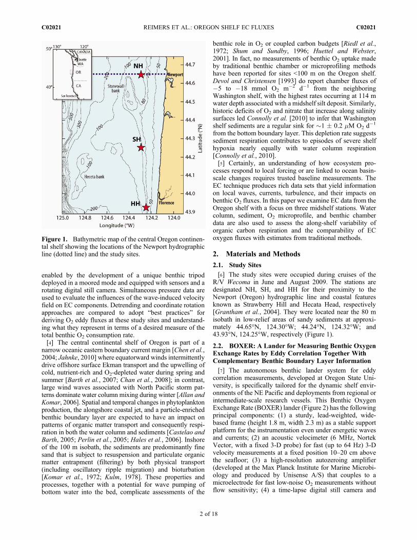
[7] The autonomous benthic lander system for eddycorrelation measurements, developed at Oregon State Uni-versity, is specifically tailored for the dynamic shelf envir-onments of the NE Pacific and deployments from regional orintermediate-scale research vessels. This Benthic OxygenExchange Rate (BOXER) lander (Figure 2) has the followingprincipal components: (1) a sturdy, lead-weighted, wide-based frame (height 1.8 m, width 2.3 m) as a stable supportplatform for the instrumentation even under energetic wavesand currents; (2) an acoustic velocimeter (6 MHz, NortekVector, with a fixed 3-D probe) for fast (up to 64 Hz) 3-Dvelocity measurements at a fixed position 10–20 cm abovethe seafloor; (3) a high-resolution autozeroing amplifier(developed at the Max Planck Institute for Marine Microbi-ology and produced by Unisense A/S) that couples to amicroelectrode for fast low-noise O2 measurements withoutflow sensitivity; (4) a time-lapse digital still camera and

Figure 1. Bathymetric map of the central Oregon continen-tal shelf showing the locations of the Newport hydrographicline (dotted line) and the study sites.

REIMERS ET AL.: OREGON SHELF EC FLUXES C02021C02021

2 of 18

strobe (Insite Pacific, Scorpio) with a counterbalancing vaneon a rotating bearing assembly for observing the seafloorareas contributing to the flux; and (5) a light level andtemperature-depth sensor (Wildlife Computers, MK-9) forindependent near-bottom measurements (mounted on topof the camera vane).[8] A newer ECmeasurement system (used for one of three

deployments) also incorporates (6) a controller unit (devel-oped by Unisense A/S) for deployment programming, power(12V, 18 h capacity by way of a rechargeable Li-ion batterypack), sensor synchronizing, calibration, and data logging(256 MB), and (7) an Aanderaa O2 optode (model 4175) forindependent O2 monitoring.[9] Prior to the introduction of the Unisense controller unit,

the Nortek Vector was used to log all data as originallyconfigured by Berg et al. [2009].[10] BOXER was deployed by lowering with Spectra

synthetic fiber line (5/8″) unwrapped from a winch drum andby releasing spar and surface buoys with an�2:1 ratio of linelength to water depth. Recovery occurred by picking up thebuoys and using the winch to haul in the line and lander.The EC instrumentation was programmed to collect data at64 Hz in 15 min bursts with 5 min between bursts. Initial andfinal bursts (i.e., those that included measurements <15 minbefore or after BOXER touched down or left the bottom)were excluded from reported data sets.

[11] The O2 microelectrode readings were stored by time(t) as counts (cts), which were converted to O2 concentra-tions according to

O2t ¼ ctst–cts0ð Þ * O2BW= ctsBW–cts0ð Þ; ð1Þ

where cts0 represents an average of predeployment readingsof the mounted sensor when dipped in a chilled (�10°C)anoxic 10% solution of 1 M Na ascorbate and 0.5 M NaOH[Andersen et al., 2001] (i.e., the zero calibration), and ctsBWequals an average set of counts recorded simultaneouslywith an independent measurement of the bottom water O2

concentration (O2BW). In this study all O2BW values wereassessed by Winkler titrations of triplicate water samplescollected within 4 m of the bottom using a conductivity-temperature-depth (CTD) probe rosette (Seabird SBE 911Plus), and ctsBW values were calculated from the averagereadings during the 15 min burst coinciding with the timeof bottom water sampling.[12] It is a unique capability of the autozeroing amplifier to

measure the constant (or DC) component of the O2 signalover a preset period at the beginning of each burst, typically30 s, and then for subsequent readings to subtract this signalfrom the total and amplify the difference 10 times, creating afluctuating (or AC) signal. Both the total and amplified ACsignals are recorded as counts. We derived O2t using themore sensitive AC records. All O2 and velocity time serieswere filtered of outliers (representing usually <1% of allmeasurements) using a phase-space method adapted fromGoring and Nikora [2002] and replaced with points based ona spline fit to adjacent data. These “cleaned” velocity and O2

time series were then reduced from 64 to 16 Hz by computingsequential four-point averages to filter out high-frequencynoise.[13] Another parameter measured by the Vector ADV is

near-bottom pressure. Pressure time series were used toextract surface wave characteristics based on finite-depthlinear water wave theory [Dean and Dalrymple, 1992].Computations were carried out in the frequency domain afterapplying a low-pass filter to the pressure spectrum witha cutoff frequency that corresponds to the shortest wavethat can still be observed by the pressure sensor (defined bylinear water wave theory as h/L = 1/2, where h is the depthof the sensor and L is the wavelength associated with awave at the cutoff frequency). All computations describedin this and following sections were executed using MatLab(Mathworks®).

2.3. EC Oxygen Flux Analysis Techniques

[14] The benthic EC oxygen flux method pioneered byBerg et al. [2003, 2009] relies on assumptions of oxygenconservation in a control volume bounded below by theseafloor and above by the intersection of the measurementpoint (zm) with an x-y coordinate plane that is parallel with theseafloor [Hume et al., 2011]. The three-dimensional tracerconservation equation for this volume and the simplifyingassumptions used in the EC technique to derive a represen-tation of the seafloor O2 source or sink are described byLorrai et al. [2010], but can also be formulated from theo-retical considerations given in papers such as those byFinnigan [1999] and Feigenwinter et al. [2004].

Figure 2. (a) Photo of the BOXER lander during deploy-ment, and (b) an enlarged view of the Vector probe posi-tioned with the O2 microelectrode and amplifier.


3 of 18

[15] To evaluate EC data sets, we first remove segments ofclearly anomalous data. These segments may be over a fewminutes up to an entire burst. Targeted anomalies are inter-vals with unusually large vertical velocities or what appear asisolated sharp dips in O2 followed by a slower return tobaseline O2 readings. The depression in the O2 signal may beexplained by marine snow or other suspended material tem-porarily adhering to the microelectrode tip. The third type ofanomaly arises when O2 shifts abruptly from having a levelmean to an increasing or decreasing trend, or vice versa,within a burst. Such shifts suggest short periods of micro-electrode instability or a changing bottom water O2 profile.[16] A following step in the EC analysis is separating the

velocity vectors and concentration measurements into time-average and fluctuating components (Reynolds decomposi-tion) [Lee et al., 2004; Lorrai et al., 2010]. Herein, we definethe time-average component to correspond to the mean overthe entire deployment and further separate the fluctuatingcomponent into a low-frequency variation and higher-frequency variability (which are presumably due to wavesand turbulence). Hence, the total time series for O2 concen-tration, for example, is then expressed as cðtÞ ¼ c þ clf ðtÞ þc′ðtÞ. Velocity components are decomposed in a similar fash-ion with the conventional notation of an overbar to denote thetime average and a prime to denote high-frequency fluctuatingcomponents. The low-frequency component is influenced bythe length and separation of individual data bursts and iden-tified using a detrending method, and the high-frequencyfluctuating component can then be obtained by subtractingthe identified mean and low-frequency components from thetotal signal. Three detrending methods are used to define thelow-frequency fluctuating component and are comparedbelow. These are (1) linear detrending (LD), (2) a centeredrunning average (RA) (see definitions given by Sakai et al.[2001] and Lee et al. [2004]), or (3) a low-pass frequencyfilter (FF) [see Bendat and Piersol, 1971, chapter 9]. Thelatter (FF) filter has some similarities to the RAmethod, but ithas the advantage of allowing for a precise understanding ofthe frequency content of the motions that are considered aspart of the high-frequency components, and it does not havecomputational edge effects at the beginning and ends ofbursts [Bendat and Piersol, 1971]. We note here that, bydefinition, the average values (over the whole deployment) ofthe fluctuating components are zero; hence c lf ¼ c′ = 0holds. Further, the average over individual bursts of the high-frequency fluctuating component also vanishes by definition.[17] The resulting net vertical flux (averaged over the

entire deployment) is

flux ¼ wc ¼ w c þ wlf clf þ w′c′: ð2Þ

When w ≠ 0; it is generally assumed that vertical advec-tion ðwcÞ does not represent a component of the seafloorexchange rate because this transport is balanced simulta-neously by transient horizontal advection events [Finniganet al., 2003]. Unfortunately, this balance cannot be con-strained from the information available from a single point inthe benthic boundary layer. The practice of coordinate rota-tion so that the mean velocity defines the x axis (and there-fore the rotated velocities are such that vR ¼ wR ¼ 0) is usedinstead by some authors to mathematically force verticaladvection terms to zero. This can be appropriate if horizontal

flow is strong and consistently at an angle relative to theseabed. The complication is with complex flow or shortaveraging periods (relative to the periods of all contributingeddies); these rotations may unpredictably fold horizontalcomponents into the eddy flux. Furthermore, rotation pro-cedures may be applied so that vR ¼ wR ¼ 0 for each sam-pling burst, creating multiple coordinate systems, or appliedonce with reference to the full data record. We examinepossible biases generated or removed by different rotationmethods as part of the results.[18] The low-frequency flux ðwlf clf Þ is generally nonzero

and, in our case, is defined to result from variability at thescales of hours to days. For example, tidal variability orchanges in the ocean properties due to upwelling fronts willcontribute to this flux. It is assumed that a sufficiently longdeployment period would capture multiple cycles of theselow-frequency motions and would therefore lead to alow-frequency flux that averages to zero in the long term. Wenote that the deployments that will be discussed herein arenot of such durations, and nonzero low-frequency fluxes areobserved.[19] Finally, the flux ðw′c′Þ in equation (2) represents all

dynamic processes that contribute a net nonzero flux ofoxygen into the seabed where it is consumed. Turbulence inthe water column undoubtedly contributes greatly to this netflux, but recent work [Huettel and Webster, 2001; Prechtet al., 2004] has suggested that processes related to surfacewave motions or flow-induced pressure gradients aroundsmall-scale sediment topography may also contribute. Forexample, wave orbital velocities near a rippled sandy bedmay lead to significant flow velocities through the bed,allowing higher rates of oxygen consumption to occur andwater of lower O2 concentration to be returned to the watercolumn [Reimers et al., 2004].[20] However, net flux computations across wave fre-

quencies can be significantly biased if the observation plat-form is not oriented perfectly in the vertical direction.Any rotation errors will result in components of the largehorizontal velocities associated with surface waves beingmapped onto the vertical velocities [Shaw and Trowbridge,2001]. Methods for removing the wave flux componentshave been under development [e.g., Shaw and Trowbridge,2001], but cannot be applied here because they require thepresence of multiple velocity sensors. Further, these methodsremove the entire wave contribution, not distinguishingbetween the real wave contribution and the apparent wavebias due to rotation errors.[21] Given our interest in the net vertical flux and the

possibility for an actual wave contribution, we instead con-sider utilizing information about the waves from the Vector’scolocated pressure sensor to adjust the orientation of theobservations. In particular, the criteria established were firstto rotate in the horizontal so the horizontal wave signal isprimarily contained in the u velocities. Hence, the x axisis aligned with the general propagation direction of thewaves. Next, a vertical rotation is established, minimizingthe difference between the observed vertical velocity (at thewave frequencies) and the vertical velocity derived via linearwater wave theory from the pressure signal. For our data sets,this amounts to a minimization of the wave signal in thevertical velocity component.


4 of 18

[22] The resulting flux term ðw′c′Þ is herein referred to asthe EC oxygen flux or eddy flux. This net flux will containcontributions from turbulence as well as from wave-inducedprocesses. These are discussed in detail as part of the results.To facilitate some understanding of the contribution of thetwo processes, the EC flux can also be expressed as

w′c′ ¼ ffmax0 Cow′c′ð f Þdf ; ð3Þ

where Cow′c′ is the cospectrum of w′c′, f is the frequency, andfmax is the upper frequency limit constrained by the samplingfrequency [Berg et al., 2003; Lorrai et al., 2010]. The signconvention is that vertical fluxes out of the base of the controlvolume and into the seabed are negative. Generally, in thisstudy we average a series of eddy flux estimates from datarecords of 14 or 14.5 min (individual 15 min bursts minus theautozeroing amplifier adjust time), resulting in a frequencyresolution of either 0.0012 or 0.0011 Hz. Cospectra are cal-culated for each burst using the Fourier transform of thefluctuating components w′ and c′ utilizing a simple Dirichletwindow. The cospectrum is then computed as the product ofthe transformed w′ and the conjugate of the transformed c′with no further band averaging.

2.4. Complementary Bottom Water and SedimentMeasurements

[23] As noted previously, we routinely conducted a CTD-rosette cast during each BOXER deployment. The CTDpackage was equipped with additional sensors, includingprobes for O2 (SBE 43) and transmissometry (Chelsea/Seatech/Wetlab CStar). The CTD was lowered to within 4 mof the seafloor and three 10 L Niskin bottles tripped in a rapidsequence (Table 1). Generally, each of these bottles wassubsampled aboard ship for O2, nutrients, and particulateorganic C and N (POC/PN) concentrations. The CTD sensordata were processed using the Sea-Bird SEASOFT softwareand laboratory calibration files to obtain 1 dbar averagevalues of pressure, temperature, conductivity, salinity, den-sity, dissolved O2 concentration, and beam transmission.Oxygen concentrations were measured by whole bottleWinkler titration of 125 ml samples using an amperometricmethod [Culberson et al., 1991] for detecting the triiodideion reaction end points. Nutrient samples were stored in acid-washed Nalgene™ 60 ml HDPE bottles at �20°C untilanalyzed using standard colorimetric methods as adapted forautoanalyzers [Atlas et al., 1971; Gordon et al., 1995]. ThePOC/PN water samples (1–1.5 L) were immediately filteredthrough precombusted (at 400°C for 4 h) 25 mmWhatman™GF/F filters. These filters were frozen at sea then laterexposed to acid fumes in the laboratory for 24 h to removeinorganic carbon. Dried filters were analyzed using a CarloErba NA-1500 elemental analyzer [Verardo et al., 1990].[24] Sediment cores (�50 cm long) were recovered

with a frame-mounted hydraulically dampened gravity corerdesigned to sample sandy sediment without pore waterdrainage and with little disturbance to the sediment-waterinterface. The acrylic core tubes (ID 10.5 cm) were 94 cm inlength, and sediment cores were retained by a spring-loaded-,“core-catcher-,” PVC disk that supported an O-ring sealagainst the tube walls. A compressed air-powered coreextruder was used in a refrigerated van (8°C� 2°C) to extrudethe sediments. For some cores, samples were collected in 1 cmT

able

1.Characteristicsof

Bottom

Water

Sam

ples

a

Statio

nDateandLocal

Tim

e(hhm

m)

Heigh

tAbo

veBottom

(m)

Oxy

genb

(mM)

POC(mM)

PN

(mM)

OC:N

a

Nitrateand

Nitrite

(mM)

Pho

sphate

(mM)

Silicate

(mM)

Ammon

ia(mM)

Salinity

Tem

perature

(°C)

Sigma-Theta

(kg/m

3)

NH

7Jun20

09,21

082.4

59.0

�0.2

9.45

�0.25

1.28

�0.10

7.4

34.4

�0.1

2.78

�0.00

63.8

�0.0

0.01

�0.01

33.92

7.03

26.57

NHc

8Jun20

09,20

292.4

60.3

�0.6

NDd

ND

ND

34.9

�0.4

2.80

�0.01

62.6

�0.3

0.02

�0.01

33.92

7.04

26.56

NH

20Aug

2009

,20

452.3

44.8

�0.3

4.58

�0.32

0.67

�0.07

6.8

34.8

�0.0

3.01

�0.03

62.8

�0.9

0.00

�0.01

33.84

7.57

26.43

SH

13Jun20

09,18

083.8

40.8

�0.2

55.36�

9.55

7.75

�0.93

7.1

32.7

�0.0

3.15

�0.06

68.2

�0.2

0.91

�0.11

33.84

7.36

26.45

SHc

18Aug

2009

,20

122.6

62.0

�0.3

10.94�

1.76

1.41

�0.23

7.8

32.4

�0.0

3.01

�0.00

63.9

�0.1

1.85

�0.02

33.86

7.71

26.43

SH

21Aug

2009

,19

531.3

62.1

�1.8

6.80

�0.38

0.96

�0.10

7.1

31.5

�0.1

2.96

�0.01

63.1

�0.5

2.23

�0.03

33.84

7.78

26.40

HHc

11Jun20

09,18

062.7

52.8

�0.1

16.58�

0.60

2.07

�0.07

8.0

33.7

�0.0

3.06

�0.05

61.5

�0.2

1.24

�0.35

33.84

7.41

26.45

a Alldiscreteanalyses

arefrom

threeindividu

alNiskinbo

ttles.T

imes

basedon

firstbo

ttlemark.

Uncertaintiesrepresent�1

SD.

bBased

onWinkler

titratio

n.c Castcoincidingwith

BOXERdeploy

ment.

dND,n

otdeterm

ined.


5 of 18

(from 0 to 5 cm) and 2 cm intervals (from 5 to 52 cm) that werethen subdivided for subsequent analyses. For other cores, onlythe top �20 cm was extruded into a 9.5 cm ID, 30 cm longacrylic core tube. This sediment was covered with seawaterfrom the study site and saved for measurements of compositepermeability in a shore-based cold room (T = 10°C � 2°C)using a falling-head permeameter designed after Rocha et al.[2005].[25] Depth profiles of excess 210Pb activity and sediment

organic C (SOC) and total N were measured after sub-sampled sediments were dried at 60°C for approximately48 h and finely ground by mortar and pestle. Approximately20 g of prepared sediment was placed in one of two CanberraGL2020RS LEGe planar (2000 mm2) g ray detectors andcounted for 24 h to determine activities of 210Pb and 214Pb(used to calculate supported 210Pb) from counts at 46.5 and661.6 keV [Wheatcroft and Sommerfield, 2005]. SOC andtotal N concentrations were measured by automated com-bustion (Carlo Erba NA1500 Series 2 elemental analyzer)with acetanilide as the calibration standard after carbonateswere removed from ground and weighed samples by con-centrated HCl fumigation (modified from Verardo et al.[1990]). Chlorophyll and phaeopigment concentrationswere determined fluorometrically after frozen sedimentsamples (2 cm3) were extracted with 90% acetone for 24 h at4°C in the dark (Turner Designs AU10) [Strickland andParsons, 1972]. Estimates of the weight percent of fines (orweight percent of silt and clay) were determined based onStokes law of particle-settling velocity. Subsamples (2 cm3)from each sediment layer were placed in 15 cm3 BD Falconconical centrifuge tubes and covered with 3 cm of filteredseawater from bottom water POC collections. After vigorousshaking, each sample was allowed to stand undisturbed for10 s, the suspension was pipetted off, and suspended particleswere collected on a preweighed filter (25 mm WhatmanGF/C). This process was repeated until the water appearedclear, usually five times per sample. The filter was thenrinsed with deionized water, wrapped securely in foil, andstored in a�80°C freezer. At a later date, filters and the sandfraction remaining in the tubes were dried and weighed.

2.5. Traditional Chamber and Microprofiler Methodsfor Estimating Benthic Oxygen Flux

[26] During each research cruise, the field plan was toassess benthic O2 fluxes by three in situ methods: EC, benthicchambers, and microelectrode profiles. Thus, two additionallanders were used in conjunction with BOXER and thehydrographic measurements. Not all lander deploymentsrecovered useful data. The benthic chamber lander wasdeployed as a free vehicle with releasable ballast. This landerinserted a pair of 20.3 � 20.3 cm box-shaped stainlesssteel chambers into the sediment. Each Teflon-lined benthicchamber was equipped with an Aanderaa model 4330 O2

optode and eight spring-actuated syringes for withdrawingtime series water samples. The optode’s output (0–5 V) wasrecorded every 5 min by the control electronics for the lander.Flux chambers were gently stirred by a 4 cm � 1 cm Teflonstir bar supported under the lid and driven by a magneticallycoupled motor at about 1 Hz. Further, description of the fluxchambers are given by Devol and Christensen [1993] andHolcombe et al. [2001]. Deployment times varied from 12 to

14 h, including delays between landing, chamber implanta-tion, and lid closure.[27] The microprofiler was mounted at the center of a

simple aluminum-frame tripod lander (1.5 m pod centerto pod center by 1.6 m high) which was deployed in the sameway as BOXER. This microprofiler has channels for four O2

microelectrodes and a four-wire resistivity sensor [Reimersand Glud, 2000]. The sensors were mounted in silicone-oil-filled holders screwed down onto a slotted anodizedaluminum ring and connected by cables to a controllingelectronics package. During this study the microprofilerwas programmed to move the sensors vertically in steps of0.125 mm, to wait 4 s at each position, then to record fromeach sensor five readings that were later averaged. Oxygenmicroelectrodes (Unisense Ox-25) were calibrated assuminga linear slope and two calibration points: an average bottomwater reading from 5 to 10 mm above the sediment-waterinterface and an average background reading in anoxic sub-surface sections of the sediment. Only two O2 microelec-trodes were used on most deployments because of a high rateof microelectrode breakage during these cruises (attributed tothe activities of Dungeness crabs seen often in sea bottomphotos). The resistivity sensor was made by embedding afour-conductor copper ribbon cable in epoxy within a plastictube and then beveling the tip into the shape of a wedgeto expose the wires along a 6 mm wide leading edge. Ithad a depth resolution of the order of 2 mm and thus beganto detect a change in resistance before encountering thesediment-water interface [Martin et al., 1991]. Resistivitymeasurements in the sediment were converted to the sedi-ment formation factor F by dividing each measurement by anaverage resistivity reading in the bottom water.

3. Results

3.1. Water Column and Eddy CorrelationMeasurements

[28] Hydrographic measurements made to coincide withthe different lander deployments showed hypoxic conditions(O2 < 64 mM or 1.43 ml/L) in the bottom waters of themidshelf region of the Oregon coast in both June and August2009. These waters were also nutrient and particle rich withT , S, and sq ranges of 7°C–8°C, 33.84–33.92, and 26.4–26.6 kg m�3, respectively, properties characteristic of thebottom mixed layer (Table 1 and Figure 3) [Perlin et al.,2005]. EC measurements were made successfully at the NHand HH sites in June and the SH site in August. These mea-surements occurred over 11–15 h (Figures 4–6). Changes inwater properties on these time scales can be attributed largelyto cross-shelf motion of bottom waters in response to tidalforcing and changes in upwelling conditions [Perlin et al.,2005]. Long-period O2 variations were greatest within theSH record and were measured by both the EC microelectrodeand independent optode (Figure 5). A pronounced bottomnepheloid layer was evident in June at both the SH and HHsites. The layer was detected by beam transmissivity values<60% near the seafloor and elevated concentrations of POCand PN (Table 1). After clipping problematic intervals fromthe EC records of Figures 4–6 (e.g., unusually large verticalvelocities in the SH data set 72 to 75 min into the record),94%, 99.5%, and 91% of the data remained for analysis forNH, SH, and HH, respectively.


6 of 18

3.2. Effects of Detrending Methods on Eddy FluxDeterminations

[29] As noted earlier, different computational and coordi-nate frame rotation methods are in common use in atmo-spheric eddy flux studies, and these same methods areavailable when investigating benthic boundary layer fluxes.Of major concern is how to separate low-frequency oscilla-tions that may bias flux calculations from those that containsignificant flux contributions [Finnigan et al., 2003]. Inaddition, a unique problem in benthic studies is how to con-sider variable surface and internal wave motions that can

dominate the turbulence-induced component of the measuredcovariance [Shaw and Trowbridge, 2001].[30] The impact of detrending methods to isolate eddy

components was first evaluated without any coordinaterotation. In Figure 7a, mean Oregon shelf eddy fluxes cal-culated after applying a RA filter to every burst period arenormalized to the mean flux calculated from the same dataafter LD. The normalized flux is shown as a function of theRA filter period, which was increased from 0.5 to 14 min.The outcome is different between data sets. The normalizedflux curve from site SH flattens near 1.0 when a 3 min or

Figure 3. Water column profiles of (a) temperature, (b) dissolved O2, and (c) percent transmission fromthe three study sites. The casts displayed coincide with BOXER deployments.

Figure 4. The full EC time series from station NH: (a, b) velocity, (c) pressure, and (d) oxygen microelec-trode data are reduced to 16 Hz. Temperature data (also in Figure 4c) from the MK-9 are at 0.067 Hz with aresolution of �0.05°C.


7 of 18

longer RA filter is applied, but the curves from NH and HHgenerally increase. This shows that detrending by LD willoften give larger-magnitude overall flux estimates until theRA period approaches the length of the data burst.[31] Both the RA and FF detrending methods indicate

greater flux contributions at frequencies <0.005 Hz withinthe NH and HH data sets compared with SH (Figures 7aand 7b). Cumulative cospectra of w′c′ examined on a burst-by-burst basis show that contributions to eddy fluxes at

frequencies <0.005 Hz are fairly persistent at HH andNH but arise more intermittently within the record fromSH. Oscillations occurring on time scales of a few minutes totens of minutes are consistent with packets of nonlinearinternal waves that are geographically and temporally vari-able sources of turbulent mixing on the Oregon shelf[D’Asaro et al., 2007]. Nonlinear internal waves have largeamplitudes and may travel long distances across the shelf,causing a net cross-shelf transport of particles [Bogucki and

Figure 6. Same as Figure 4 except the data are for HH.

Figure 5. The full EC time series from station SH. The Unisense controller system with optode was usedduring this deployment. (a, b) Velocity, (c) pressure, and (d) oxygen microelectrode data are reduced to16 Hz. Optode oxygen measurements (in Figure 5d) are at 1 Hz, and temperature readings from theMk-9 sensor (in Figure 5c) are at 0.017 Hz.


8 of 18

Redekopp, 1999]. These phenomena may also explain why insome bursts the lower-frequency portion of cospectra reducesrather than enhances the overall eddy flux estimate of O2

consumption, and this makes the outcome very sensitive todetrending methods. An example is illustrated by data from440.5 to 455 min into the HH time series. The eddy fluxderived from this data segment equals �2.85,�7.8,�8.6, or�9.2 mmol m�2 d�1, depending on whether detrending is byLD, 0.002 Hz FF, 8.33 min RA, or 4 min RA computations,respectively (Figure 8, curve set 1). In contrast, for the burstfrom 280.5 to 295 min, the same series of fluxes equals�22.4, �12.5, �16.8, and �13.1 mmol m�2 d�1, in partbecause oscillatory trends in this data segment appear to havea period greater than the burst duration (Figure 8, curve set 2).

[32] Figure 8 also illustrates the cutoff behavior of the FFin comparison with other detrending methods in nonrotateddata from HH. As frequency contributions approaching0.001 Hz are both negative and positive in these records, itmay be advantageous for there to be a long time series overwhich these effects will tend to average out. This could beaccomplished in the future by having much longer burstsor here by averaging over many bursts. Selecting only a few10–15 min bursts to represent overall eddy fluxes couldmisrepresent the strength of the seafloor sink in this envi-ronment. These points will be returned to below.

3.3. Coordinate Rotation Influences

[33] A consistent pattern in these EC data sets is that w isnonzero and negative (Table 2). Possible causes for this areinstrument leveling errors that introduce horizontal flowcontributions into w [Pond, 1968; Shaw and Trowbridge,2001], complex flow patterns that cause short-term ensem-bles of mean velocity vectors to orient at an angle relative tothe seabed [Finnigan et al., 2003], flow deflection by com-ponents of the BOXER framework or sensor supports, orripple- or other permeable bed form-induced effects on thenear-bed velocity field under waves [Doering and Baryla,2002]. Since the Vector contains a compass and tilt meter,these measurements show that the greatest measure ofinstrument pitch or roll was 4.1° at NH, but these angles were<0.5° at SH and HH. Assuming a nearly level seabed, thisimplicates complex flow, frame interference, and/or bed formeffects at these stations. The practice of rotating coordinatesso that vR ¼ wR ¼ 0 over each burst is arguably best suitedfor cases in which there is an instrument leveling error orsteady flow at an angle relative to the bottom boundary andhas been used by Berg and Huettel [2008] and Berg et al.[2009]. Rotation results from all three sites show that thisrotation method can both increase and decrease apparentfluxes on a burst-by-burst basis. At stations NH and SH, theoverall effect is to decrease the magnitude of the averageeddy flux (e.g., 53%–61% compared with nonrotated withLD), whereas at HH the magnitude is enhanced (52% com-pared with nonrotated with LD) and the range for all bursts isgreatly expanded (Table 3).[34] Finnigan et al. [2003] suggest that in situations with

long-period fluctuations, a complication of rotating coordi-nates every period is an introduction of horizontal compo-nents into w′c′ rather than their removal. This seemsespecially likely if the forced rotation angle in the vertical(i.e., around the horizontal axis) is larger than a few degreesas it became for most individually rotated bursts (e.g., at HHthe range was �28.2° to �2.6° with a mean of �6.6°). Onealso sees an enhanced surface wave signal in wR when suchrotated time series are plotted on top of nonrotated data (notshown). These analyses cause us to reject this method ofrotating coordinates every period as appropriate for benthicEC measurements of this nature.[35] Alternatively, a single rotation defined by the

requirement that vR ¼ wR ¼ 0 only over an entire long-termdata record could be applied to fix a new coordinate frame.Such a rotation scheme is best applied when there is astrong current from one direction. Nonetheless, we havedone this for the three Oregon shelf data sets, and the effectis much the same, with rotation angles in the vertical of

Figure 7. (a) Average fluxes derived after detrending usinga centered running average (RA) with increasing filter periodnormalized to the flux derived after linear detrending (LD).(b) Fluxes after applying a low-pass frequency filter (FF) ofincreasing cutoff frequency normalized to the flux derivedafter LD. Each point represents an average from all databursts after removing some anomalous data segments andwithout rotation of axes (see text).


9 of 18

�10° to 16° and most bursts showing an enhanced wavesignal in wR.[36] Instead, what seems most appropriate is to rotate the

coordinates using information extracted from u, v, w and thepressure signal to minimize any wave bias in wR (asdescribed in section 2.3). The resulting qV angles are small,vary little from burst to burst (�2.1° � 0.7°, �1.5° � 2.9°,and 0.9° � 0.6° for NH, SH, and HH, respectively), and areclose to the compass angles. The highest variability isobserved at SH, where the horizontal rotation angle variesalso, likely because of the turbulent nature of the velocities(also see section 3.4). A comparison of eddy fluxes derivedwith and without this final rotation is presented in Table 3. Asrotation effects are not independent of detrending, fluxespredicted after this rotation are also compared with LD, RA,and FF methods. We highlight the combination of lineardetrending with the rotation to minimize wave biasing as the“preferred” to represent the strength of the seafloor sinkbecause with these �15 min burst segmented data sets thistreatment both retains more low-frequency contributionswithin the eddy flux (i.e., last term of equation (2)) andminimizes wave contamination. In effect, we are making thejudgment that because data bursts were <15 min and sepa-rated by 5 min gaps in time, the best method to retain realwave fluctuations with periods of several minutes to hours iswith linear detrending. If the data had been collected in lon-ger bursts or a long-duration continuous mode instead, a low-

pass frequency filter would probably be preferable because itcould be adjusted to precisely remove very low frequencies(e.g., <�0.0001 Hz; in other words, fluctuations due to long-period exchanges such as tides).[37] Figure 9 shows the burst-to-burst variability of the

preferred flux estimates, reflected as �1 standard deviation(SD) in Table 3. Cumulative averages in Figure 9 illustratethat several hours of measurements are needed to approach aconsistent flux estimate. The drivers of the apparent vari-ability on shorter time scales are discussed in section 4.

3.4. “Real” Surface Wave Contributions toEddy Fluxes

[38] The significant wave heights (Hsig) and average waveperiods (Tp) derived from the pressure records of each ECtime series were typical for late spring and summer condi-tions (Table 2). Surface wave observations from the NationalData Buoy Center (NDBC) buoy off Newport (buoy 46050)indicate that during the HH deployment, waves were small(significant wave height Hsig � 0.8 m), and the waves werecharacterized by swell (peak period Tp � 16 s) from thesouthwest. Similar waves were present during the NHdeployment; however, in addition, NDBC data also give anindication of a secondary sea peak at around an 8 s period.In contrast, during the SH deployment, short-period waves(Tp � 8 s) were dominant, and associated wave heights werelarger (Hsig � 2 m) and approaching from the northwest.

Figure 8. Cumulative cospectra of w′c′ from HH data segments spanning 440.5–455 min (point 1) and280.5–295 min (point 2), computed with df = 0.0011 Hz, no rotation of axes, and with linear, low-pass filter(cutoff = 0.002 Hz), or running average (periods = 4 and 8.33 min) detrending methods.

Table 2. Means �1 SD (Minimum to Maximum) of Vertical and Horizontal Velocities (cm s�1) and Wave Conditions Derived OverEach Data Burst and Averaged Across All Burstsa

Site Number of Bursts Mean Vertical Velocity �w Mean Velocityb (cm/s) Hsig (m) Tp (s)

NH 35 �0.51 � 0.30 (�0.98 to +0.03) 5.8 � 2.7 (0.3 to 10.4) 0.45 � 0.03 13.9 � 1.6SH 44 �0.40 � 0.19 (�0.83 to +0.04) 3.8 � 1.2 (0.8 to 6.7) 0.44 � 0.10 11.1 � 1.2HH 45 �0.39 � 0.17 (�1.05 to �0.12) 4.1 � 2.5 (0.3 to 13.4) 0.60 � 0.08 15.3 � 0.9

aSignificant wave heights (Hsig) and periods (Tp) reflect only those surface waves sensed near the seafloor.bAbsolute value of resultant of u, v, and w at measuring height above bottom of Vector.


10 of 18

Table 3. Comparison of the Effects of Coordinate Frame Rotation (Each Period) and Mean Removal Method on O2 Eddy Fluxes DerivedFrom Measurements in This Studya

Site and Number of Bursts Rotation Mean Removal Total Eddy Flux (w′c′) Wave Frequency Eddy Flux

NH, n = 33 none LD �4.4 � 3.1 �1.26 � 0.99vR ¼ wR ¼ 0 LD �1.7 � 3.5 �0.69 � 1.15

Minimize wave bias LD �3.2 � 3.2 �0.53 � 0.94Minimize wave bias RA (8.33 min) �3.0 � 3.2 �0.53 � 0.95Minimize wave bias RA (4 min) �2.4 � 2.5 �0.53 � 0.95Minimize wave bias FF (0.002 Hz) �2.4 � 3.0 �0.53 � 0.99Minimize wave bias FF (0.005 Hz) �1.9 � 2.5 �0.53 � 0.99

SH, n = 44 none LD �4.3 � 4.1 �0.53 � 0.74vR ¼ wR ¼ 0 LD �2.0 � 6.3 �0.37 � 0..90

Minimize wave bias LD �3.9 � 3.9 �0.52 � 0.65Minimize wave bias RA (8.33 min) �3.8 � 3.6 �0.52 � 0.65Minimize wave bias RA (4 min) �3.7 � 2.9 �0.52 � 0.65Minimize wave bias FF (0.002 Hz) �3.4 � 4.6 �0.53 �0.68Minimize wave bias FF (0.005 Hz) �3.5 � 3.4 �0.53 �0.68

HH, n = 42 none LD �13.0 � 16.2 �4.1 � 4.3vR ¼ wR ¼ 0 LD �19.8 � 32.5 �12.2 � 17.6

Minimize wave bias LD �9.8 � 14.9 �2.3 � 3.8Minimize wave bias RA (8.33 min) �10.0 � 13.5 �2.3 � 3.8Minimize wave bias RA (4 min) �8.7 � 11.6 �2.3 � 3.8Minimize wave bias FF (0.002 Hz) �9.0 � 12.1 �2.3 � 3.8Minimize wave bias FF (0.005 Hz) �8.1 � 10.6 �2.3 � 3.8

aAll fluxes are burst averages in mmol m�2 d�1 (�1 SD to reflect the variability between individual bursts that is due to the flow dynamics). Here 6% of therecord from NH, 0.5% from SH, and 9% from HH were excluded from these analyses for reasons given in the text. Boldface values are preferred for reasonsgiven in the text. LD, linear detrending; RA, running average filter; FF, a low-pass frequency filter.

Figure 9. Eddy fluxes of O2 (mmol m�2 d�1) by burst at (a) NH, (b) SH, and (c) HH. These estimateswere derived after rotating coordinates to minimize wave biasing and using linear detrending. The dashedred lines represent averages accumulated with increasing number of bursts.


11 of 18

However, at the water depth of the EC measurements (80–85 m), waves shorter than approximately 10 s cannot beobserved because of the depth attenuation associated withsurface gravity waves.[39] The EC observations show that during the HH (and

NH) deployments, oscillations transferred from passing sur-face waves are most pronounced in u and v. Horizontalvelocities derived from the pressure observations are con-sistently in good agreement with the measured velocities(r2 values of 0.9 and 0.8 for HH and NH, respectively),indicating that the observed motions are indeed mostlyassociated with surface gravity waves, with the remainingenergy likely due to turbulent motions. Signals associatedwith the surface gravity waves are also visible in O2 timeseries. Oscillations were much less sinusoidal during theSH deployment, and this is apparent in spectral analyses(Figure 10). The observed motions at wave frequencies at SHdo not appear as organized swell with a clear propagationdirection (r2 values between pressure-derived velocities andobservations were only 0.2, with an equally large standarddeviation from burst to burst). Further, frequency spectraderived from the pressure observations clearly indicate thatthe peak wave frequency cannot be captured because thewaves are much shorter during this deployment and hencecannot be observed at these water depths. Instead, themotions measured during the SH deployment are likely pri-marily due to turbulence, leading to relatively large ampli-tude fluctuations in w. Without rotation, contributions to totalfluxes at NH and HH are clearly heightened at wave fre-quencies (Figure 7b). After rotation to remove wave biases,the contributions from the dominant surface wave frequency

bands to the total EC oxygen fluxes are reduced but stillequal to a significant 13%–23% overall (Table 3). Thesewere calculated over a 0.05 Hz frequency band centered at1/Tp (as in Table 2). Mean currents were variable in direc-tion with speeds of <14 cm/s (Table 2).

3.5. Comparability of Eddy Fluxes With Chamberand Microprofile Methods

[40] Confidence in the validity of equating eddy fluxes tothe seafloor sink for O2 can best be obtained by comparisonwith established benthic flux methods and by considering therelative strengths and weakness of all methods. In this studywe were successful in determining alternative estimates ofthe benthic O2 flux by deploying a benthic chamber landerand a microprofiler lander at both NH and SH, althoughcontemporaneous measurements by all three methodswere achieved only at SH in August (Table 4). Results ofside-by-side chamber incubations over 10 h at SH(Figure 11b) show variant trends, but when the sedimentuptake of O2 is estimated from linear fits over the first180 min, the chamber fluxes are equal to �4.6 � 0.5 and�7.2� 0.7 mmol m�2 d�1 in June and August, respectively.NH chamber fluxes measured in August were more consis-tent between chambers (Figure 11a) and equal to �5.8 �0.2 mmol m�2 d�1 (Table 4).[41] Water-sediment profiles measured in situ at NH

and SH with O2 microelectrodes and a resistivity sensor areshown in Figure 12. Although there is only a single O2 pro-file for each deployment (due to either companion sensorbreakage or poor-quality records), we have measured sim-ilar profiles at other Oregon shelf stations (C. E. Reimers,

Figure 10. (a, e) Power spectra of vertical velocity w, (b, f) O2 concentration C with (c, g) cospectra ofw′C′, and (d, h) cumulative cospectra of w′C′ from representative EC data bursts from stations HH andSH. The HH example is from the deployment time interval 740.5–755 min, and the SH example is from300.5 to 315 min.


12 of 18

Table 4. Summary of Lander Deployments and Coring Stations From Which Data and Comparative Oxygen Fluxes Are Reported

SiteCollection Date, Time,

and Typeb

Position

Water Depth (m)Total or Diffusive OxygenFlux (mmol m�2 d�1)Latitude (°N) Longitude (°W)

NH 7 Jun 2009, 1921, IMP 44° 39.042′ 124° 17.722′ 82 �1.1NH 8 Jun 2009, 1959, BOXER 44° 39.097′ 124° 18.005′ 82 �3.2 (see Table 3)HH 11 Jun 2009, 1533, BOXER 43° 55.800′ 124° 14.705′ 80 �9.8 (see Table 3)SH 13 Jun 2009, 1458, Chambers 44° 14.033 124° 18.924 82 �4.6 � 0.5 (n = 2)SH 18 Aug 2009, 1600, BOXER 44° 14.511′ 124° 18.930′ 81 �3.9 (see Table 3)NH 20 Aug 2009, 1843, Chambers 44° 39.398′ 124° 18.006′ 82 �5.8 � 0.2 (n = 2)NH 20 Aug 2009, 2022, IMP 44° 39.099′ 124° 17.750′ 81 �2.7SH 21 Aug 2009, 1700, Chambers 44° 14.701′ 124° 18.896′ 81 �7.2 � 0.7 (n = 2)SH 21Aug 2009, 1922, IMP 44° 14.515′ 124° 18.871′ 81 �2.4

SiteCollection Date, Time,

and Typeb

Position

Water Depth (m)Permeability or Sampling

HistoryLatitude (°N) Longitude (°W)

NH 7 Jun 2009, 1501, Corer 44° 38.940′ 124° 18.000′ 83 sectioned into 1 and 2 cm intervalsNH 7 Jun 2009, 1518, Corer 44° 38.949′ 124° 18.001′ 83 1.74 (�0.09) � 10�11 m2a

SH 18 Aug 2009, 1636, Corer 44° 13.321′ 124° 19.047′ 81 1.76 (�0.08) � 10�10 m2

SH 18 Aug 2009, 1653, Corer 44° 13.321′ 124° 19.049′ 81 sectioned into 1 and 2 cm intervalsHH 11 Jun 2009, 1936, Corer 43° 56.094′ 124° 14.994′ 81 sectioned into 1 and 2 cm intervals

aFour replicate measurements of permeability were made per core. Uncertainties represent �1 SD.bTime given as local time.

Figure 11. Dissolved oxygen concentration versus time in benthic chambers during NH and SHdeployments. C1, chamber 1; C2, chamber 2. Oxygen was measured by optodes mounted in the chamberlids. These records start at the time of chamber closure, which occurred 3–5 h after deployment. Chamberfluxes are derived from linear fits to the O2 consumption over the first 180 min.


13 of 18

unpublished data, 2009), and so have confidence that theseare typical for summer hypoxic conditions. The steep inter-facial gradients do not indicate any deep O2 intrusion due toflow- or wave-induced advection and can be used with Fick’sfirst law as it is often applied to sediments: DOU ¼ � Do

F∂C∂z ,

whereDo is the molecular diffusion coefficient for O2 at in situtemperatures and F is the formation factor of interfacial sedi-ment [Ullman and Aller, 1982; Schulz, 2006] to derive diffu-sive O2 fluxes equal to �1.1, �2.7, and �2.4 mmol m�2 d�1

at NH in June, NH in August, and SH in August 2009,respectively (Table 4). However, we fully expect DOU cal-culations to underestimate the total flux. As demonstrated byGüss [1998], purely hydrodynamic dispersion can enhancethe O2 uptake near the interface of permeable sediments byseveral times molecular diffusion without much deepeningof the O2 penetration. These potential effects, in addition torespiration of macrofauna and biological pore water irriga-tion, imply that both the EC and chamber oxygen fluxes arerealistic representations of total oxygen consumption rates.

3.6. Sediment Properties Driving Variabilityin Eddy Fluxes

[42] The most striking variability in average eddy fluxesderived for the three shelf sites is the greater flux at HHcompared with the two sites further north. As water depth,bottom water O2 concentrations, and temperature werelargely consistent during these three deployments and waveconditions were similar between HH and NH, we look to thesediments for another source of the variability. The collectioninformation for sediment cores that were analyzed for thisstudy is presented in Table 4 with measurements of com-posite permeability (sites NH and SH only). Profiles of sed-iment properties downcore are displayed in Figure 13. Thereis little to distinguish the HH site except for its relativelyhigher percentages of fines and organic carbon content.Concentrations of excess 210Pb are low at all sites (especially

in comparison with shelf muds) and indicate that the top�7 cm of the three sites have comparable histories of win-nowing and bioturbation. Chlorophyll-a is generally enri-ched at the sediment surface, but chlorophyll-to-phaeophytinmolar ratios (averaging 0.31 � 0.12 and not shown) changelittle with sediment depth or between cores.

4. Discussion

4.1. Assessment of Fluxes

[43] Although the derivation of benthic fluxes from ECmeasurements may be described in straightforward steps[e.g., Kuwae et al., 2006; Lorrai et al., 2010], in practice thisstudy shows that not all data sets are simple, and the outcomefrom EC can be sensitive to the methods used to orientcoordinates and split measurements into mean and fluctuat-ing components. On the Oregon continental shelf, becausevelocities were dominated by wave motions rather than bycurrents and because measurements were made in a rela-tively short burst mode, we find that the most defendablefluxes are derived by (1) orienting the coordinate axes tominimize surface wave biasing of the vertical velocity and(2) applying linear detrending methods to retain within theeddy contributions the lowest frequencies sampled per burst(0.0011 Hz in this study). This processing does not removeall the flux contributions at surface wave frequencies (asseen in Figure 10 and Table 3), but what remains is inferredto be due to real wave- or pressure-driven exchange pro-cesses that transport bottom water enriched in oxygen intoat least the uppermost millimeters of a permeable seabedand oxygen-depleted pore water out [Precht et al., 2004].With relatively short data bursts (<15 min), the longest-period oscillations that may be incorporated into the ECoxygen flux are on the time scales of internal waves, whichare known to enhance turbulence on the Oregon continentalshelf [D’Asaro et al., 2007]. Bioirrigation may be anothermechanism to produce low-frequency components in O2

Figure 12. Profiles of O2 and sediment formation factor measured in situ at (a) NH in June, (b) NH inAugust, and (c) SH in August 2009.


14 of 18

spectra (Figure 10). Low-pass frequency filter analyses witha cutoff frequency of 0.005 Hz when compared with LD(Table 3) indicate contributions at frequencies of <0.005 Hzcarried about 41%, 10%, and 17% of total EC oxygenfluxes assessed from the NH, SH, and HH deployments,respectively. In contrast, real contributions at surface wavefrequencies were assessed as equal to 17%, 13%, and 23%,respectively (Table 3). This implies that between 42% and77% of measured eddy fluxes arose from turbulent eddiesat typical near-bottom frequencies [Shaw and Trowbridge,2001].[44] Another important conclusion is that because of low-

frequency oscillations, conservation may in fact hold over thecourse of only a relatively long time series (at least severalhours). This means that only when averaged over such longtime scales can eddy fluxes correctly represent the seafloorsink. Said in other terms, the sometimes large variabilitybetween the eddy fluxes derived for individual bursts(Figure 9) is because internal waves or other low-frequencymixing events cause intermittent advection or flux diver-gence contributions to continuity [see also Brand et al., 2008;McGinnis et al., 2011]. This reasoning is why we cautionreaders to be cognizant that the short-term variability of the

eddy fluxes as reported in Table 3 is not a measure thatshould be used to infer whether fluxes are significantly dif-ferent between sites. In essence, we consider n = 1 for eachBOXER deployment (Table 4), and the results of replicatedeployments are required before statistical tests concerningmean fluxes are attempted.[45] The smaller magnitudes of the eddy flux assessments

of O2 uptake compared with those of chambers, both ofwhich are greater (as expected) than diffusive flux estimatesfrom O2 microelectrode profiles, are results that differ frompast comparison studies in marine environments with sandysediments. For example, Berg and Huettel [2008] found anaverage nighttime O2 uptake assessed by EC to be 3.8 timesthe rate derived from diver-deployed cylindrical chambersin a shallow (�1 m depth) nearshore site in ApalachicolaBay, Florida. In the Florida study, the three velocity com-ponents were rotated so that wR → 0 every burst; however,the resulting eddy flux was not highly sensitive to changes incoordinate orientation. We suspect that shallow sites likeApalachicola Bay, which are under nearly air-saturatedwaters and experience regularly strong tidal currents, exhibita greater degree of advective oxygen flux enhancement thanthe �80 m Oregon shelf sites we have studied under late

Figure 13. Profiles of sediment properties from cores: (a) wt % fines, (b) wt % organic C, (c)chlorophyll-a, and (d) excess 210Pb.


15 of 18

spring and summer conditions. Flux contributions due topore water pumping through a few to tens of centimeters ofhighly permeable sediment are not easily measured by ben-thic chambers [Jahnke et al., 2005]. However, more workwill need to be done to fully understand the effects of fluxmethodology, water depth, and physical variables onexchange processes involving such permeable sediments.[46] In this study, the only contemporaneous comparison

of O2 flux methods was at SH. The observed eddy-to-chamber flux ratio of 0.54 may indicate that the chamberssampled a localized “hot spot” within the Oregon shelf ben-thos such as has been documented on other margins andascribed to an inhomogeneous distribution of decomposingphytodetritus [e.g., as in Glud et al., 2009]. Additionally,chamber methods have their own sources of error and bias-ing. As reviewed by Reimers et al. [2001] and Viollier et al.[2003], among the potential concerns are (1) changes in thehydrodynamic regime, including the diffusive sublayeradjacent to the sediment surface; (2) artificially inducing orblocking advective pore water flow (especially with perme-able sediments); and (3) artifacts caused by chambers dis-turbing the water and sediment layers to be studied. Thechambers used in this study were square and relatively small(0.04 m2), but have yielded O2 and silicate fluxes that agreedwithin a factor of 2 with a wide variety of other designsduring an intercalibration study [Tengberg, 1997]. Glud andBlackburn [2002] argue that insertion of small chambers will,per area of sediment, damage a greater number of fauna andburrows, which could enhance the O2 flux. These effectsshould be proportionally greater when overall O2 fluxes arelow. The nonlinear O2 traces (Figure 11) suggest a changingsediment-water interface gradient as the overlying waterconcentration decreases and (at SH) some divergent behav-ior, probably caused by different irrigation or bioturbationrates of benthic fauna.[47] Our results do show an increase in eddy fluxes at 80 m

moving from north off Newport to south off Hecata Headunder similar late spring and summer conditions. This lati-tudinal trend is probably the best evidence that the eddyfluxes are valid representations of benthic O2 consumptionrates in this region. The water column and sediments to thesouth were observed to be richer in organic carbon, indicat-ing sources of both fresh and buried organic matter tointensify rates of O2 utilization. A pronounced bottomnepheloid layer was also evident at station HH in June.Cross-shelf motion of these near-bottom layers in responseto changes in tides and upwelling-relaxation cycles hasbeen described by Perlin et al. [2005], but it is not knownhow the variable turbulence and particulate loads of theselayers couple to benthic biogeochemical cycling. There isan indication that regions of high turbidity are associatedwith regions of higher turbulence stemming in part frominternal waves generated in areas of rough topography[D’Asaro et al., 2007]. Barth et al. [2005] describe a low-temperature, high-salinity, turbid bottom water pool, sup-plied primarily from the south in the lee region inshoreof Heceta Bank and speculate that this region could be rela-tively important in the generation of low-O2 waters on theshelf through local respiration. Our measurements supportthis possibility and suggest a need for additional flux mea-surements in the vicinity and farther south of HH.

4.2. The Contribution of Benthic Oxygen Consumptionto Hypoxia

[48] Hypoxia at shelf depths in late spring and summer onthe Oregon continental margin is indicated to be a new phe-nomenon that may signal an ecosystem response to changesin upwelling wind stress from climate warming [Granthamet al., 2004; Chan et al., 2008]. It is debated whether moresevere hypoxia has arisen because of a greater contributionof low-O2 source waters to the shelf or instead from greaterin situ drawdown of O2 through respiration in the benthicboundary layer including the sediments [Connolly et al.,2010]. Encompassing our measurements, current meter anddissolved O2 records from a moored platform at 70 m adja-cent to SH showed that hypoxic conditions persisted inthe bottom boundary layer for over two-thirds of the timebetween mid-April and mid-September 2009 (K. Adams andJ. Barth, personal communication, 2011). During the sameperiod, there were four major wind-driven upwelling eventsfollowed by intervals of wind relaxation and downwelling.As a consequence, at midshelf depths, cumulative alongshore currents were relatively weak, which extended the localresidence time of a density-confined bottom boundary layer(K. Adams and J. Barth, personal communication, 2011).Longer residence times of bottom boundary waters on theshelf should facilitate O2 depletion by the sedimentary sink.[49] The measurements reported here provide a baseline

range for total seafloor O2 utilization rates of approximately3 to 10 mmol m�2 d�1. Using these rates, benthic respirationcan be expected to deplete O2 at a rate on the order of 1 mMd�1

from the bottom 5–10 m of the water column, which matchesrates estimated for water column respiration and for sedi-mentary O2 consumption from mass balances of dissolvedO2 and nitrate in near-bottom waters by Connolly et al.[2010] for the Washington shelf. In the future, we hope todocument how sensitive benthic O2 fluxes are to bottomwater O2 concentrations, water depth, and the internal andsurface wave conditions in this region. However, comparedwith other marine environments of similar water depths[Glud, 2008], the benthic O2 consumption rates measuredso far on the Oregon shelf are lower than average (theregression of global data of Glud [2008, Figure 16] predictsa typical total O2 utilization rate = 11 mmol m�2 d�1 fora depth = 80 m). The relatively low rates suggest that(1) hypoxic conditions create a negative feedback (i.e., lowerbottom water O2 leads to a lower O2 consumption rate)[Eldridge and Morse, 2008] and (2) the recent rise in shelfhypoxia along the U.S. West Coast is not because local res-piration rates have increased in response to climate forcing.Rather, shelf hypoxia appears in response to more persistent(but interannually variable) upwelling-relaxation cycles thatcombine to inject O2-depleted source waters onto the shelf,then hold these waters in the bottom boundary in contact withthe benthic sink for O2.

5. Summary and Conclusions

[50] This study presents sediment oxygen uptake ratesdetermined from eddy correlation measurements madeusing a new lander (BOXER) designed for deployments fromresearch vessels and investigations of continental shelfenvironments. When the lander was applied off centralOregon at �80 m depth in June 2009, surface wave (swell


16 of 18

with a peak period Tp � 16 s) impacts on variations invertical velocities and O2 were strongly evident, while inAugust 2009 surface waves were much shorter and hencethe variations measured were primarily due to turbulence.[51] Three detrending methods (linear, centered running

average, and low-pass frequency filter) were compared,leading to the assessment that linear detrending is mosteffective when data bursts are of durations similar to thoseof important nonturbulent motions such as internal waves.However, if longer data bursts or continuous records arecollected in future studies, a low-pass frequency filter set toeliminate long-period fluctuations would have the advantageof more precisely defining the frequencies of dynamic pro-cesses included in EC fluxes. Furthermore, records of pres-sure variations were shown to be useful for establishingcoordinate rotation angles that minimize the contaminationof vertical velocity components with horizontal componentsof wave motion.[52] The EC O2 fluxes determined ranged between �3 and

�10 mmol m�2 d�1 while benthic chamber O2 fluxes mea-sured in duplicate at just two of the stations ranged between�4 and �8 mmol m�2 d�1. All fluxes are too low to impli-cate an intensification of local diagenetic processes for agreater prevalence of hypoxic conditions in the benthicboundary layer of the Oregon shelf during the last decade.However, local depletion rates may be sensitive to a numberof local variables such as water depth, the dynamics ofinternal mixing, bottom water O2, sediment permeability,ripple regime, and sediment organic matter content. It is ourintention to examine these controls more comprehensivelyin future research.

[53] Acknowledgments. We thank the officers and crew of the R/VWecoma for ensuring the successful execution of this research. Oregon StateUniversity Marine Technicians Daryl Swensen and David O’Gorman con-tributed greatly to the deployment strategy and provided critical equipmentrepairs while at sea. We thank Jay Simpkins and Tim Nolan for design andconstruction of the BOXER lander. Lars Damsgaard, from Unisense A/S,provided dedicated support of the EC equipment and its development for thisresearch. Cody Doolan, Joe Jennings, Margaret Sparrow, Yvan Alleau, andSteve Pierce provided invaluable help with collecting and analyzing thewater column and sediment data reported. Wendi Ruef and Bonnie Changprovided technical support of the benthic chambers. Rob Wheatcroft pro-vided use of his lab’s gamma ray detectors. Support for this project was pro-vided by the National Science Foundation under grants OCE 0726984 and1061218 to C. Reimers and is gratefully acknowledged. A. Devol’s partici-pation was supported by NSF grant OCE 0628391. The paper was improvedafter receiving helpful reviews from Richard Dewey, Filip Meysman, CecileCathalot, and an anonymous reviewer.

ReferencesAllan, J. C., and P. D. Komar (2006), Climate controls on US west coasterosion processes, J. Coastal Res., 22, 511–529, doi:10.2112/03-0108.1.

Andersen, K., T. Kjær, and N. P. Revsbech (2001), An oxygen insensitivemicrosensor for nitrous oxide, Sens. Actuators B, 81, 42–48, doi:10.1016/S0925-4005(01)00924-8.

Atlas, E. L., S. Hager, L. Gordon, and P. Park (1971), A practical manual ofuse of the Technicon AutoAnalyzer in seawater nutrient analyses, Rev.Oreg. State Univ. Tech. Rep. 215, Dept. of Oceanogr., Oreg. State Univ.,Corvallis.

Aubinet, M. (2008), Eddy covariance CO2 flux measurements in nocturnalconditions: An analysis of the problem, Ecol. Appl., 18(6), 1368–1378,doi:10.1890/06-1336.1.

Barth, J. A., S. D. Pierce, and R. M. Castelo (2005), Time-dependent, wind-driven flow over a shallow mid-shelf submarine bank, J. Geophys. Res.,110, C10S05, doi:10.1029/2004JC002761.

Barth, J. A., B. A.Menge, J. Lubchenco, F. Chan, J. M. Bane, A. R. Kirinich,M. A. McManus, K. J. Nielsen, S. D. Pierce, and L. Washburn (2007),Delayed upwelling alters nearshore coastal ocean ecosystems in the

northern California current, Proc. Natl. Acad. Sci. U. S. A., 104,3719–3724, doi:10.1073/pnas.0700462104.

Bendat, J. S., and A. G. Piersol (1971), Random Data: Analysis andMeasurement Procedures, 407 pp., Wiley-Interscience, New York.

Berg, P., and M. Huettel (2008), Monitoring the seafloor using the noninva-sive eddy correlation technique: Integrated benthic exchange dynamics,Oceanography, 21, 164–167, doi:10.5670/oceanog.2008.13.

Berg, P., H. Røy, F. Janssen, V. Meyer, B. B. Jørgensen, M. Huettel, andD. de Beer (2003), Oxygen uptake by aquatic sediments measured witha novel non-invasive eddy-correlation technique, Mar. Ecol. Prog. Ser.,261, 75–83, doi:10.3354/meps261075.

Berg, P., H. Røy, and P. Wiberg (2007), Eddy correlation flux measure-ments: The sediment surface area that contributes to the flux, Limnol.Oceanogr., 52, 1672–1684, doi:10.4319/lo.2007.52.4.1672.

Berg, P., R. N. Glud, A. Hume, H. Stahl, K. Oguri, V. Meyer, andH. Kitazato (2009), Eddy correlation measurements of oxygen uptakein deep ocean sediments, Limnol. Oceanogr. Methods, 7, 576–584,doi:10.4319/lom.2009.7.576.

Bogucki, D., and L. G. Redekopp (1999), A mechanism for sedimentresuspension by internal solitary waves, Geophys. Res. Lett., 26(9),1317–1320, doi:10.1029/1999GL900234.

Brand, A., D. F. McGinnis, B. Wehrli, and A. Wüest (2008), Intermittentoxygen flux from the interior into the bottom boundary of lakes asobserved by eddy correlation, Limnol. Oceanogr., 53, 1997–2006,doi:10.4319/lo.2008.53.5.1997.

Castelao, R. M., and J. A. Barth (2005), Coastal ocean response to summerupwelling favorable winds in a region of alongshore bottom topographyvariations off Oregon, J. Geophys. Res., 110, C10S04, doi:10.1029/2004JC002409.

Chan, F., J. A. Barth, J. Lubchenco, A. Kirincich, H. A.Weeks,W. H. Peterson,and B. A. Menge (2008), Emergence of anoxia in the California Currentlarge marine ecosystem, Science, 319, 920, doi:10.1126/science.1149016.

Chen, C.-T. A., A. Andreev, K.-R. Kim, and M. Yamamoto (2004), Rolesof continental shelves and marginal seas in biogeochemical cyclesof the North Pacific Ocean, J. Oceanogr., 60, 17–44, doi:10.1023/B:JOCE.0000038316.56018.d4.

Connolly, T. P., B. M. Hickey, S. L. Geier, and W. P. Cochlan (2010), Pro-cesses influencing seasonal hypoxia in the northern California CurrentSystem, J. Geophys. Res., 115, C03021, doi:10.1029/2009JC005283.

Culberson, C. H., G. Knapp, M. C. Stalcup, R. T. Williams, and F. Zemlyak(1991), A comparison of methods for the determination of dissolved oxy-gen in sea water,WHP Office Rep. WHPO-91–2, World Ocean Circ. Exp.Hydrogr. Prog. Off., La Jolla, Calif.

D’Asaro, E. A., R.-C. Lien, and F. Henyey (2007), High-frequency inter-nal waves on the Oregon continental shelf, J. Phys. Oceanogr., 37,1956–1967, doi:10.1175/JPO3096.1.

Dean, R. G., and R. A. Dalrymple (1992),Water Wave Mechanics for Engi-neers and Scientists, 353 pp., World Sci., Teaneck, N. J.

Devol, A. H., and J. P. Christensen (1993), Benthic fluxes and nitrogencycling in sediments of the continental margin of the eastern NorthPacific, J. Mar. Res., 51, 345–372, doi:10.1357/0022240933223765.

Doering, J. C., and A. J. Baryla (2002), An investigation of the velocityfield under regular and irregular waves over a sand beach, CoastalEng., 44, 275–300, doi:10.1016/S0378-3839(01)00037-0.

Eldridge, P., and J. Morse (2008), Origins and temporal scales of hyp-oxia on the Louisiana shelf: Importance of benthic and sub-pycnoclinewater metabolism, Mar. Chem., 108, 159–171, doi:10.1016/j.marchem.2007.11.009.

Feigenwinter, C., C. Bernhofer, and R. Vogt (2004), The influence ofadvection on the short term CO2-budget in and above a forest canopy,Boundary Layer Meteorol., 113, 201–224, doi:10.1023/B:BOUN.0000039372.86053.ff.

Finnigan, J. J. (1999), A comment on the paper by Lee (1998), “On micro-meteorological observations of surface-air exchange over tall vegeta-tion,” Agric. For. Meteorol., 97, 55–64, doi:10.1016/S0168-1923(99)00049-0.

Finnigan, J. J., R. Clement, Y. Malhi, R. Leuning, and H. A. Cleugh (2003),A re-evaluation of long-term flux measurement techniques. Part I: Aver-aging and coordinate rotation, Boundary Layer Meteorol., 107, 1–48,doi:10.1023/A:1021554900225.

Glud, R. N. (2008), Oxygen dynamics of marine sediments,Mar. Biol. Res.,4, 243–289, doi:10.1080/17451000801888726.

Glud, R. N., and N. Blackburn (2002), The effect of chamber size onbenthic oxygen uptake measurements: A simulation study, Ophelia, 56,23–31.

Glud, R. N., H. Stahl, P. Berg, F. Wenhöfer, K. Oguri, and H. Kitazato(2009), In situ microscale variation in distribution and consumption ofO2: A case study from a deep ocean margin sediment (Sagami Bay,Japan), Limnol. Oceanogr., 54, 1–12, doi:10.4319/lo.2009.54.1.0001.


17 of 18

Glud, R. N., P. Berg, A. Hume, P. Batty, and M. E. Blicher (2010), BenthicO2 exchange rates across hard-bottom substrates quantified by eddycorrelation in a sub-Arctic fjord system, Mar. Ecol. Prog. Ser., 417,1–12, doi:10.3354/meps08795.

Gordon, L. I., J. C. Jennings, A. R. Ross, and J. M. Krest (1995) A sug-gested protocol for continuous flow automated analysis of seawater nutri-ents (phosphate, nitrate, nitrite, and silicic acid) in the WOCEHydrographic Program and the Joint Global Ocean Fluxes Study, Oreg.State Univ. Tech. Rep.93–1, Oreg. State Univ., Corvallis.

Goring, D. G., and V. I. Nikora (2002), Despiking acoustic Doppler velo-cimeter data, J. Hydraul. Eng., 128, 117–126, doi:10.1061/(ASCE)0733-9429(2002)128:1(117).

Grantham, B. A., F. Chan, K. J. Nielsen, D. S. Fox, J. A. Barth, J. Huyer,J. Lubchenco, and B. A. Menge (2004), Upwelling-driven nearshorehypoxia signals ecosystem and oceanographic changes in the northeastPacific, Nature, 429, 749–754, doi:10.1038/nature02605.

Güss, S. (1998), Oxygen uptake at the sediment water interface simulta-neously measured using a flux chamber method and microelectrodes:Must a diffusive boundary layer exist?, Estuarine Coastal Shelf Sci.,46, 143–156, doi:10.1006/ecss.1997.0265.

Hales, B., L. Karp-Boss, A. Perlin, and P. A. Wheeler (2006), Oxygen pro-duction and carbon sequestration in an upwelling coastal margin, GlobalBiogeochem. Cycles, 20, GB3001, doi:10.1029/2005GB002517.

Holcombe, B. L., R. G. Kiel, and A. H. Devol (2001), Determination ofpore-water dissolved organic carbon fluxes from Mexican margin sedi-ments, Limnol. Oceanogr., 46, 298–308, doi:10.4319/lo.2001.46.2.0298.

Huettel, M., and I. T. Webster (2001), Porewater flow in permeable sedi-ments, in The Benthic Boundary Layer: Transport Processes and Biogeo-chemistry, edited by B. P. Boudreau and B. B. Jørgensen, pp. 144–177,Oxford Univ. Press, New York.

Hume, A. C., P. Berg, and K. J. McGlathery (2011), Dissolved oxygenfluxes and ecosystem metabolism in an eelgrass (Zostera marina)meadow measured with the eddy correlation technique, Limnol. Ocea-nogr., 56, 86–96, doi:10.4319/lo.2011.56.1.0086.

Jahnke, R. A. (2010), Global synthesis, in Carbon and Nutrient Fluxes inContinental Margins, Intl. Geosphere-Biosphere Prog. Ser., vol. 28, edi-ted by K. K. Liu et al., chap. 16, pp. 597–616, Springer, Berlin.

Jahnke, R., M. Richards, J. Nelson, C. Robertson, A. Rao, and D. Jahnke(2005), Organic matter remineralization and porewater exchange ratesin permeable South Atlantic Bight continental shelf sediments, Cont.Shelf Res., 25, 1433–1452, doi:10.1016/j.csr.2005.04.002.

Komar, P. D., R. H. Neudeck, and L. D. Kulm (1972), Observations andsignificance of deep-water oscillatory ripple marks on the Oregon conti-nental shelf, in Shelf Sediment Transport: Process and Patterns, editedby D. J. P. Swift, D. B. Duane, and O. H. Pilkey, pp. 601–619, Dowden,Hutchinson and Ross, Stroudsburg, Penn.

Kulm, L. D. (1978), Coastal morphology and geology of the ocean bottom-the Oregon region, in The Marine Plant Biomass of the Pacific NorthwestCoast, edited by R. Krauss, pp. 9–35, Oregon State Univ. Press,Corvallis.

Kuwae, T., K. Kamio, T. Inoue, E. Miyoshi, and Y. Uchiyama (2006), Oxy-gen exchange flux between sediment and water in an intertidal sandflat,measured in situ by the eddy-correlation method, Mar. Ecol. Prog. Ser.,307, 59–68, doi:10.3354/meps307059.

Lee, X., W. Massman, and B. Law (2004), Handbook of Micrometeorology:A Guide for Surface Flux Measurement and Analysis, Kluwer Acad.,Dordrecht, Netherlands.

Lorrai, C., D. F. McGinnis, P. Berg, A. Brand, and A. Wüest (2010), Appli-cation of oxygen eddy correlation in aquatic systems, J. Atmos. OceanicTechnol., 27, 1533–1546, doi:10.1175/2010JTECHO723.1.

Martin, W. R., M. Bender, M. Leinen, and J. Orchard (1991), Benthicorganic carbon degradation and biogenic silica dissolution in the centralequatorial Pacific, Deep Sea Res. Part A, 38, 1481–1516, doi:10.1016/0198-0149(91)90086-U.

McGinnis, D. F., P. Berg, A. Brand, C. Lorrai, T. J. Edmonds, andA. Wüest (2008), Measurements of eddy correlation oxygen fluxes inshallow freshwaters: Towards routine applications and analysis, Geophys.Res. Lett., 35, L04403, doi:10.1029/2007GL032747.

McGinnis, D. F., S. Cherednichenko, S. Sommer, P. Berg, L. Rovelli,R. Schwarz, R. N. Glud, and P. Linke (2011), Simple, robust eddy corre-lation amplifier for aquatic dissolved oxygen and hydrogen sulfide fluxmeasurements, Limnol. Oceanogr. Methods, 9, 340–347, doi:10.4319/lom.2011.9.340.

Perlin, A., J. N. Moum, and J. Klymak (2005), Response of the bottomboundary layer over a sloping shelf to variations in alongshore wind,J. Geophys. Res., 110, C10S09, doi:10.1029/2004JC002500.

Pond, S. (1968), Some effects of buoy motion on measurements of windspeed and stress, J. Geophys. Res., 73(2), 507–512, doi:10.1029/JB073i002p00507.

Precht, E., U. Franke, L. Polarecky, and M. Huettel (2004), Oxygendynamics in permeable sediments with wave-driven pore water exchange,Limnol. Oceanogr., 49, 693–705, doi:10.4319/lo.2004.49.3.0693.

Reimers, C. E., and R. N. Glud (2000), In situ chemical sensor measure-ments at the sediment-water interface, in Chemical Sensors in Oceanog-raphy, edited by M. S. Varney, pp. 249–282, Gordon and Breach,Amsterdam.

Reimers, C. E., R. A. Jahnke, and L. Thomsen (2001), In situ sampling inthe benthic boundary layer, in The Benthic Boundary Layer: TransportProcesses and Biogeochemistry, edited by B. P. Boudreau and B. B.Jørgensen, pp. 245–268, Oxford Univ. Press, New York.

Reimers, C. E., H. A. Stecher III, G. L. Taghon, C. M. Fuller, M. Huettel,A. Rusch, N. Ryckelynck, and C. Wild (2004), In situ measurements ofadvective solute transport in permeable shelf sands, Cont. Shelf Res.,24, 183–201, doi:10.1016/j.csr.2003.10.005.

Riedl, R. J., N. Huang, and R. Machan (1972), The subtidal pump: a mech-anism of interstitial water exchange by wave action,Mar. Biol. Berlin, 13,210–221, doi:10.1007/BF00391379.

Rocha, C., S. Forster, E. Koning, and E. Epping (2005), High-resolutionpermeability determination and two-dimensional porewater flow in sandysediment, Limnol. Oceanogr. Methods, 3, 10–23, doi:10.4319/lom.2005.3.10.

Sakai, R. K., D. R. Fitzjarrald, and K. E. Moore (2001), Importance oflow-frequency contributions to eddy fluxes observed over roughsurfaces, J. Appl. Meteorol., 40, 2178–2192, doi:10.1175/1520-0450(2001)040<2178:IOLFCT>2.0.CO;2.

Schulz, H. D. (2006), Quantification of early diagenesis: Dissolved con-stituents in marine pore water and signals in the solid phase, inMarine Geochemistry, 2nd ed., edited by H. D. Schulz and M. Zabel,pp. 73–124, Springer, Berlin, doi:10.1007/3-540-32144-6_3.

Shaw, W. J., and J. H. Trowbridge (2001), The direct evaluation of near-bottom turbulent fluxes in the presence of energetic wave motions,J. Atmos. Oceanic Technol., 18, 1540–1557, doi:10.1175/1520-0426(2001)018<1540:TDEONB>2.0.CO;2.

Shum, K. T., and B. Sundby (1996), Organic matter processing in conti-nental shelf sediments—The subtidal pump revisited, Mar. Chem., 53,81–87, doi:10.1016/0304-4203(96)00014-X.

Strickland, J. D. H., and T. R. Parsons (1972), A Practical Handbook ofSeawater Analysis, 2nd ed., Fish. Res. Board of Can., Ottawa, Canada.

Tengberg, A. (1997), Free-vehicle benthic lander technology for the studyof biogeochemical processes in marine sediments, PhD thesis, ChalmersUniv. of Technol., Göteborg, Sweden.

Ullman, W. J., and R. C. Aller (1982), Diffusion coefficients in nearshoremarine sediments, Limnol. Oceanogr., 27, 552–556, doi:10.4319/lo.1982.27.3.0552.

Verardo, D. J., P. N. Froelich, and A. McIntyre (1990), Determination oforganic carbon and nitrogen in marine sediments using the Carlo ErbaNA-1500 analyzer, Deep Sea Res. Part A, 37, 157–165, doi:10.1016/0198-0149(90)90034-S.

Viollier, E., et al. (2003), Benthic biogeochemistry: State of the art technol-ogies and guidelines for the future of in situ survey, J. Exp. Mar. Biol.Ecol., 285–286, 5–31, doi:10.1016/S0022-0981(02)00517-8.

Wheatcroft, R. A., and C. K. Sommerfield (2005), River sediment flux andshelf sediment accumulation rates on the Pacific Northwest margin, Cont.Shelf Res., 25, 311–332, doi:10.1016/j.csr.2004.10.001.

P. Berg, Department of Environmental Sciences, University of Virginia,PO Box 400123, Clark Hall, Balcony, Charlottesville, VA 22904, USA.A. Devol, School of Oceanography, University of Washington, PO

Box 355351, Seattle, WA 98195-7940, USA.K. McCann-Grosvenor, H. T. Özkan-Haller, C. E. Reimers, and R. D.

Sanders, College of Oceanic and Atmospheric Sciences, Oregon StateUniversity, 104 COAS Administration Bldg., Corvallis, OR 97331, USA.([email protected])


18 of 18

Documents

Benthic oxygen consumption rates during hypoxic conditions ... · oxygen consumption rates during hypoxic conditions on the Oregon continental shelf: Evaluation of the eddy correlation