Automatic evaluation of FHR recordings fromCTU-UHB CTG database

Jirı Spilka1 George Georgoulas2 Petros Karvelis2 Vangelis P. Oikonomou2

Vaclav Chudacek1 Chrysostomos Stylios2 Lenka Lhotska1 Petr Janku3

1 Dept. of Cybernetics, Czech Technical University in Prague, Czech Republic2 Dept. of Informatics and Communications Technology, TEI of Epirus, Arta, Greece3 Dept. of Gynecology and Obstetrics, Teaching Hospital of Masaryk University in

Brno, Czech Republicspilka.jiri@fel.cvut.cz

Abstract. Fetal heart rate (FHR) provides information about fetal well-being during labor. The FHR is usually the sole direct information chan-nel from the fetus – undergoing the stress of labor – to the clinician whotries to detect possible ongoing hypoxia. For this paper, new CTU-UHBCTG database was used to compute more than 50 features. Featurescame from different domains ranging from classical morphological fea-tures based on FIGO guidelines to frequency-domain and non-linear fea-tures. Features were selected using the RELIEF (RELevance In Estimat-ing Features) technique, and classified after applying Synthetic MinorityOversampling Technique (SMOTE) to the pathological class of the data.Nearest mean classifier with adaboost was used to obtain the final re-sults. In results section besides the direct outcome of classification thetop ten ranked features are presented.

Keywords: fetal heart rate, intrapartum, feature selection, classifica-tion

1 Introduction

Electronic fetal monitoring (EFM) is used for fetal surveillance during preg-nancy and, more importantly, during delivery. The EFM most commonly refersto cardiotocography (CTG) that is a measurement of fetal heart rate (FHR)and uterine contractions (UC). Since its introduction the CTG has served as themain information channel providing obstetricians with insight into fetal well-being. CTG monitoring still plays a role of the most prevalent method in use formonitoring of antepartum as well as intrapartum fetal well-being. The goal offetal monitoring is to prevent fetus of potential adverse outcomes and provide aninformation about his/hers well-being. The main advantage of CTG, when com-pared to previously used auscultation technique, lies in its ability of continuousfetal surveillance though, this advantage is claimed to be insignificant in pre-venting adverse outcomes (with exception of neonatal seizures) as described inmeta-analysis of several clinical trials [1]. The other main controversies of CTG

include: increased rate of cesarean sections [1] and high intra- and inter-observervariability [2, 3].

Nowadays CTG remains the most prevalent method for intrapartum fetalsurveillance [2, 4], often supported by ST-analysis (Neoventa Medical, Sweden)which is based on analysis of fetal electrocardiogram (FECG). The introductionof additional ST-analysis into the clinical practice improved the labor outcomesslightly [5, 6] but its use is not always possible or feasible since it requires invasivemeasurement. Moreover, in order to use ST-analysis the correct interpretationof CTG is still required.

The interpretation of CTG is based on FIGO guidelines [7] introduced in1986, or their newer international alternatives [8]. The main goal of guidelines isto assure lowering of the number of asphyxiated neonates while keeping the num-ber of unnecessary cesarean sections (due to false alarms) at possible minimum.Additional goal of the guidelines was to lower the high inter and intra-observervariability. Despite the efforts made, the variability of clinicians evaluation ofCTG still persists [9]. Three possible ways to lower it were discussed. e.g. [10] i)by extensive training, ii) using the most experienced clinician as an oracle, iii)and/or by computerized system supporting clinicians with the decision process.

The attempts of computerized CTG interpretation are almost as old as theFIGO guideline themselves. Beginning with work of [11] the automatic analy-sis of CTG was aligned with clinical guidelines [12]. Beyond the morphologicalfeatures used in the guidelines, new features were introduced for FHR analysis.These were mostly based on the research in the adult heart rate variability [13].The statistical description (time domain) of CTG tracings was employed in [14]and in [15]. The spectrum of FHR either in antepartum or intrapartum periodoffered insight to fetal physiology, and the short review [16] described recentdevelopment in this area. The joint time-frequency analysis of FHR in the formof wavelet analysis was employed in [17]. Nonlinear methods are widely used forFHR analysis [18, 19] and in our recent work we showed their usefulness in thisfield [20]. Different approaches were used for classification of FHR into differentcategories either based on pH levels, base deficit, or other clinical parameters.These approaches includes: Support Vector Machines ( SVMs) [17, 21, 20], artifi-cial neural networks (ANNs) [22, 23], or a hybrid approach utilizing grammaticalevolution [24].

The contributions of the paper are twofold: First, from the CTG point ofview, the used database will be open access at the time of publication, This isone of the largest databases used for automatic evaluation of the CTG. Second,we provide a promising approach for the automatic classification of CTG usingthe umbilical pH value as a gold standard. The results could serve as a basemethodology for a new algorithm development on clinically sound data. Anoverview of the procedure is shown in Fig. 1.

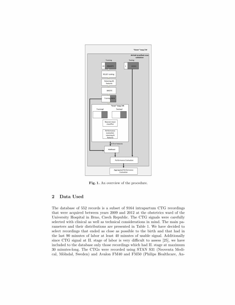
Fig. 1. An overview of the procedure.

2 Data Used

The database of 552 records is a subset of 9164 intrapartum CTG recordingsthat were acquired between years 2009 and 2012 at the obstetrics ward of theUniversity Hospital in Brno, Czech Republic. The CTG signals were carefullyselected with clinical as well as technical considerations in mind. The main pa-rameters and their distributions are presented in Table 1. We have decided toselect recordings that ended as close as possible to the birth and that had inthe last 90 minutes of labor at least 40 minutes of usable signal. Additionallysince CTG signal at II. stage of labor is very difficult to assess [25], we haveincluded to the database only those recordings which had II. stage at maximum30 minutes-long. The CTGs were recorded using STAN S31 (Neoventa Medi-cal, Molndal, Sweden) and Avalon FM40 and FM50 (Philips Healthcare, An-

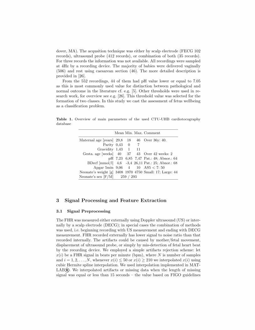
dover, MA). The acqusition technique was either by scalp electrode (FECG 102records), ultrasound probe (412 records), or combination of both (35 records).For three records the information was not available. All recordings were sampledat 4Hz by a recording device. The majority of babies were delivered vaginally(506) and rest using caesarean section (46). The more detailed description isprovided in [26].

From the 552 recordings, 44 of them had pH value lower or equal to 7.05as this is most commonly used value for distinction between pathological andnormal outcome in the literature cf. e.g. [5]. Other thresholds were used in re-search work, for overview see e.g. [26]. This threshold value was selected for theformation of two classes. In this study we cast the assessment of fetus wellbeingas a classification problem.

Table 1. Overview of main parameters of the used CTU-UHB cardiotocographydatabase

Mean Min. Max. Comment

Maternal age [years] 29,8 18 46 Over 36y: 40.Parity 0,43 0 7

Gravidity 1,43 1 11Gesta. age [weeks] 40 37 43 Over 42 weeks: 2

pH 7,23 6,85 7,47 Pat.: 48; Abnor.: 64BDecf [mmol/l] 4,6 -3,4 26,11 Pat.: 25; Abnor.: 68

Apgar 5min 9,06 4 10 AS5 < 7: 50Neonate’s weight [g] 3408 1970 4750 Small: 17; Large: 44Neonate’s sex [F/M] 259 / 293

3 Signal Processing and Feature Extraction

3.1 Signal Preprocessing

The FHR was measured either externally using Doppler ultrasound (US) or inter-nally by a scalp electrode (DECG); in special cases the combination of methodswas used, i.e. beginning recording with US measurement and ending with DECGmeasurement. FHR recorded externally has lower signal to noise ratio than thatrecorded internally. The artifacts could be caused by mother/fetal movement,displacement of ultrasound probe, or simply by mis-detection of fetal heart beatby the recording device. We employed a simple artifacts rejection scheme: letx(i) be a FHR signal in beats per minute (bpm), where N is number of samplesand i = 1, 2, . . . , N , whenever x(i) ≤ 50 or x(i) ≥ 210 we interpolated x(i) usingcubic Hermite spline interpolation. We used interpolation implemented in MAT-LAB®. We interpolated artifacts or missing data when the length of missingsignal was equal or less than 15 seconds – the value based on FIGO guidelines

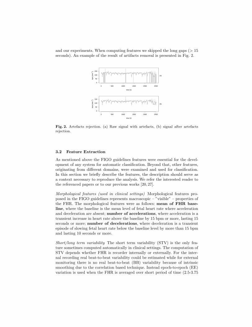
and our experiments. When computing features we skipped the long gaps (> 15seconds). An example of the result of artifacts removal is presented in Fig. 2.

0 500 1000 1500 2000 2500

0

50

100

150

time [s]

bpm

[min

--1]

(a)

0 500 1000 1500 2000 2500

0

50

100

150

time [s]

bpm

[min

--1]

(b)

Fig. 2. Artefacts rejection. (a) Raw signal with artefacts, (b) signal after artefactsrejection.

3.2 Feature Extraction

As mentioned above the FIGO guidelines features were essential for the devel-opment of any system for automatic classification. Beyond that, other features,originating from different domains, were examined and used for classification.In this section we briefly describe the features, the description should serve asa context necessary to reproduce the analysis. We refer the interested reader tothe referenced papers or to our previous works [20, 27].

Morphological features (used in clinical settings) Morphological features pro-posed in the FIGO guidelines represents macroscopic – ”visible” – properties ofthe FHR. The morphological features were as follows: mean of FHR base-line, where the baseline is the mean level of fetal heart rate where accelerationand deceleration are absent; number of accelerations, where acceleration is atransient increase in heart rate above the baseline by 15 bpm or more, lasting 15seconds or more; number of decelerations, where deceleration is a transientepisode of slowing fetal heart rate below the baseline level by more than 15 bpmand lasting 10 seconds or more.

Short/long term variability The short term variability (STV) is the only fea-ture sometimes computed automatically in clinical settings. The computation ofSTV depends whether FHR is recorder internally or externally. For the inter-nal recording real beat-to-beat variability could be estimated while for externalmonitoring there is no real beat-to-beat (BB) variability because of intrinsicsmoothing due to the correlation based technique. Instead epoch-to-epoch (EE)variation is used when the FHR is averaged over short period of time (2.5-3.75

sec.). Recall that x(i) is the i-th FHR sample in beat per minute (bpm), let T (i)a FHR sample in milliseconds i = 1, 2, . . . , N , where N is the length of FHR.As noted in [28] the STV computed using x(i) and T (i) is not always the samebecause of dependence on the value of FHR mean utilized in some variabilitycomputation. The STV is estimated for signals of length 60 sec.; for longer signalsthe 60 sec. estimations are averaged. There exist several methods for comput-ing STV and LTV, a comparison could be found in [28]. Here we present onlya short list: STVavg estimated as the average of successive beat differences:STV = 1

N

∑N−1i=1 |T (i+ 1)− T (i)| [ms], STV-DeHann estimated as the inter

quartile range of angular differences between successive T (i)s [29], SDNN [13],STV-Yeh [30], and Sonicaid 8000 [31]. Long term variability (LTV) featureswere computed over 60 seconds and there was no need of averaging the FHRin 60 seconds. For FHR signals longer than 60 sec. estimations of LTV wereaveraged over each 60 sec. LTV-DeHaan [29] and the Delta value [14]. Manyof the above mentioned features have been used in cases of antepartum signalevaluation and the effectiveness of many of them depends on their performancein the presence of accelerations and decelerations.

Frequency domain features Various spectral methods have been used for the anal-ysis of adult heart rate [13]. In the case of FHR analysis, no standardized use offrequency bands exists. Therefore we used two slightly different partitionings ofthe frequency bands as was previously used in our work [21]. First we divided thefrequency range into 3 bands [13] and calculated the energy of the signal in eachone of them: Very Low Frequency (VLF); Low Frequency (LF) referredto as Mayer waves and High Frequency (HF) corresponding to fetal move-ment. Additionally the ratio of energies in the bands: ratio LF HF = LF

HF wascomputed. It is a standard measure in adults and expresses the balance of be-havior of the two autonomic nervous system branches. The alternative frequencypartitioning followed suggestions of [32]. They proposed the following 4 bands:Very Low Frequency (VLF); Low Frequency (LF) correlated with neuralsympathetic activity; Movement Frequency (MF), related to fetal movementsand maternal breathing; High Frequency (HF), marking the presence of fetalbreathing. Similarly to the previous 3-band division the following ratio of energieswas computed: ratio LF MFHF = LF

MF+HF . This ratio is supposed to quantifythe autonomic balance control mechanism (in accordance with the LF/HF rationormally calculated in adults). The spectrum of FHR was estimated using thefast Fourier transform.

Nonlinear features Almost all nonlinear methods used for FHR analysis havetheir roots in adult HRV research. For nonlinear features we detrened FHRby the estimated baseline and also normalized the signal to have zero meanand unit variance. The Poincare plot is a basic nonlinear feature commonlyused in HRV domain [13]. The plot is a geometric representation of HRV whereeach RR interval is plotted as a function of the previous one. In this work weestimated waveform fractal dimension by several methods. These were: box-counting dimension, which expresses the relationship between the number

of boxes that contain part of a signal and the size of the boxes; the Higuchimethod (FD Hig) [33], where the curve length 〈L(k)〉 is computed for differentsteps k and it is related to the fractal dimension by an exponential formula; thevariance fractal dimension (FD Var) that is based on properties of frac-tional Brownian motion. The variance sigma2 is related to the time increments∆t of a signal X(t) according to the power law [34]; an estimate of the fractal di-mension proposed by Sevcik [35]; Detrend Fluctuations Analysis (DFA) [36] forestimating the fractal dimension, D, via scaling exponent α, D = 3− α. For allmethods, the fractal dimension was estimated as the slope of a fitted regressionto log-log plot of, e.g. for Higuchi method 〈L(k)〉 versus k. Also we estimatedtwo scaling regions corresponding to STV and LTV, respectively [33]. The sep-aration (critical) time was 3s. In addition, in order to estimate both regions byone parameter, we also fitted the log-log plot with a second order polynomialwhich coefficients (first order and second order polynomial coefficient) corre-spond to the both STV and LTV. The Approximate Entropy (ApEn) is ableto distinguish between low-dimensional deterministic systems, chaotic systems,stochastic and mixed systems [37]. ApEn(m,r) approximately equals the averageof a natural logarithm of conditional probabilities that sequences of length m areclose to each other, within a tolerance r, even if a new point is added. A slightlymodified estimation of approximate entropy was proposed by [38] and resulted inSample Entropy (SampEn). This estimation overcame the shortcomings ofthe ApEn mainly because the self-matches were excluded. The used parametersfor ApEn and SampEn estimation are: tolerance r = (0.15; 0.2) ·SD (SD standsfor standard deviation) and the embedding dimension m = 2 [39] The last of thenonlinear features was the Lempel Ziv Complexity (LZC) [40]. This methodexamines reoccurring patterns contained in the time series irrespective of time.A periodic signal has the same reoccurring patterns and low complexity whilein random signals individual patterns are rarely repeated and signal complexityis high.

3.3 Feature Selection

Usually in most pattern recognition applications the feature extraction stage isfollowed by a feature selection stage [41] which reduces the input dimensional-ity, because in real world applications we tend to extract more features thannecessary in an effort to include all possible information. However, sometimessome of the extracted features can be correlated, hence redundant information islikely to be included or sometimes some features are irrelevant to the applicationat hand and may negatively affect the performance of the classifier. The term”performance” refers to the training time required during the construction of theclassification model or, which is the more serious side-effect, the discriminativecapability of the classifier. In feature selection, a search problem of finding asubset of l features from a given set of d features, l < d has to be solved in orderto optimize a specific evaluation measure, i.e the performance of the classifier.There are a number of approaches that try to tackle this problem which can

roughly be divided into three categories: filters, wrappers and embedded meth-ods [42]. The filter approach ranks features based on a performance evaluationmetric calculated directly from the data; the wrapper approach employs a pre-dictive model and uses its output to determine the quality of the selected featuresand the embedded approach integrates the selection of features in model build-ing. In this work a hybrid approach combining a filter and a wrapper approachwas combined. More specifically RELevance In Estimating Features (RELIEF)was employed to rank the features and then based on the ranking the number ofretained features was determined by directly estimating their performance usinga predictive model. In the rest of the section we briefly present RELIEF whereasthe wrapped stage is explained in more detail in Section 4.

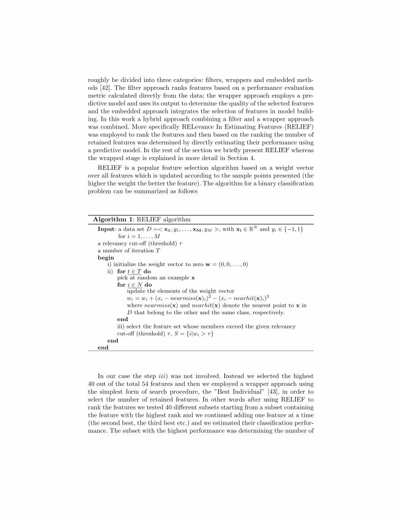
RELIEF is a popular feature selection algorithm based on a weight vectorover all features which is updated according to the sample points presented (thehigher the weight the better the feature). The algorithm for a binary classificationproblem can be summarized as follows

Algorithm 1: RELIEF algorithm

Input: a data set D =< x1, y1, . . . ,xM, yM >, with xi ∈ RN and yi ∈ {−1, 1}for i = 1, . . . ,M

a relevancy cut-off (threshold) τa number of iteration Tbegin

i) initialize the weight vector to zero w = (0, 0, . . . , 0)ii) for t ∈ T do

pick at random an example xfor i ∈ N do

update the elements of the weight vectorwi = wi + (xi − nearmiss(x)i)

2 − (xi − nearhit(x)i)2

where nearmiss(x) and nearhit(x) denote the nearest point to x inD that belong to the other and the same class, respectively.

endiii) select the feature set whose members exceed the given relevancycut-off (threshold) τ , S = {i|wi > τ}

endend

In our case the step iii) was not involved. Instead we selected the highest40 out of the total 54 features and then we employed a wrapper approach usingthe simplest form of search procedure, the ”Best Individual” [43], in order toselect the number of retained features. In other words after using RELIEF torank the features we tested 40 different subsets starting from a subset containingthe feature with the highest rank and we continued adding one feature at a time(the second best, the third best etc.) and we estimated their classification perfor-mance. The subset with the highest performance was determining the number of

features involved in the estimation performance phase as it is will be presentedin more detail in the next Section 4.

4 Classification Procedure

As it was pointed out in section 2, one class, the abnormal one, is heavily under-sampled in comparison to the normal one. This creates an extra challenge tothe already difficult task of fetus well-being diagnosis. The class imbalance isa fundamental problem, arising when pattern recognition methods are dealingwith real life problems, and many approaches have been proposed to overcomethis situation [44]. In order to compensate for this imbalance we employed apopular technique which operates on the minority class creating artificial data,the Synthetic Minority Oversampling TEchnique (SMOTE). SMOTE is basedon real data belonging to the minority class and it operates in the feature spacerather than the data space [45]. The algorithm for each instance (in feature space)of the minority class introduces a synthetic example along any/all of the linesjoining that particular instance with its k nearest neighbors that belong to theminority class. Usually after SMOTE the training set has approximately equalnumbers of the 2 classes. However in this study our preliminary results suggestedthat more synthetic data from the minority class were needed. Therefore weselected to oversample the minority class by a factor of 18 using 27 (k=27)neighbors without trying to further optimize/tune the parameter settings ofSMOTE. For testing the classification performance by making use of as manyof the abnormal instances as possible we applied a 44 fold (stratified) crossvalidation procedure with each fold containing 1 abnormal instance and 12 or11 normal instances. Therefore each time 43 abnormal instances were used fortraining and 496 or 497 normal instances and 1 abnormal instance and 12 (11)normal instances were saved for testing. During each fold we applied SMOTE tothe abnormal instances, with the aforementioned parameters, while the normalinstances remained intact. After the application of SMOTE an ”inner” loopinvolved for the selection of the ”optimal” number of features. During every foldRELIEF used all the training data (not the synthetic ones) to rank the featuresand then an inner loop was executed 4 times during which the data was randomlydivided into training and testing (70/30) and a classifier was tested using 1 to40 features (starting with the best feature and adding one feature at a timebased on its ranking). Based on the average classification accuracy over thesefour repetitions the ”optimal” number of features was selected. After selectingthe number of retained features, the whole training set (with the inclusion of thedata coming from the SMOTE stage) was used to train a classifier to be testedon the reserved testing set. In this work we employed the simplest member of thenearest prototype classifier family, the nearest mean prototype classifier, whichassigns an instance to the class whose mean vector is closest to, during the innerloop procedure, and after that (after the selection of the number of features toretain) we employed the same classifier but within the adaboost framework inorder to come up with a more powerful classification scheme. Adaboost which

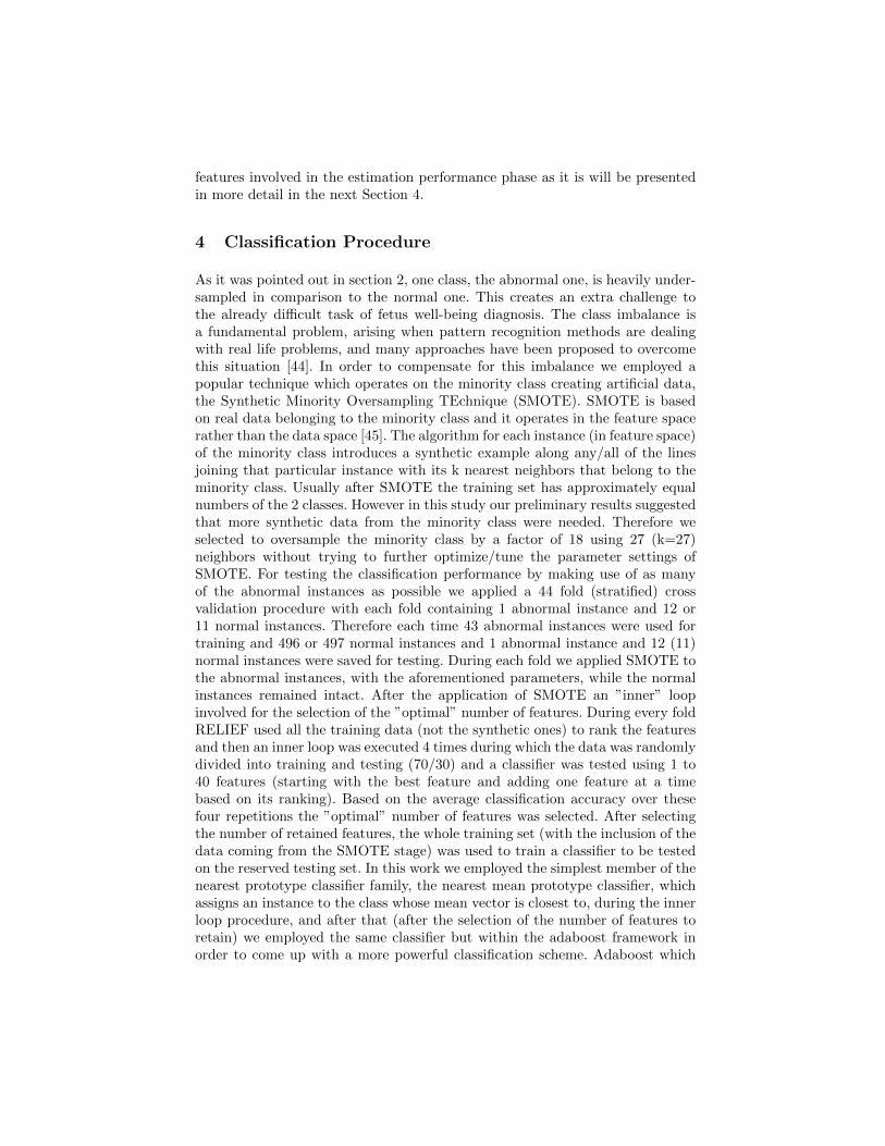
comes from adaptive boosting was first introduced by Freund and Schapire [46] isa general method for improving the performance of a week learner. It is the mostwell-known model guided instance selection for building ensemble classifiers. Thebasic steps of the algorithm are summarized as follows (following mainly thenotation provided in [47]).

Algorithm 2: Adaboost algorithm

Input: a data set D =< x1, y1, . . . ,xM, yM >, with xi ∈ RN and yi ∈ {−1, 1}for i = 1, . . . ,M

kmax – the maximum number of weak learners to be included in the ensembleC – a weak learnerbegin

i) initialize the weight vector W1 = (1/M, 1/M, . . . , 1/M)ii) for k = 1, . . . , kmax do

train weak learner Ck sampling D according to Wk

ek ←∑i:Ck(xi)6=yi

Wk(i), where Ck(x) is the output of the weakclassifier for instance xαk ← 1

2ln(

1−ekek

)Wk+1(i)← Wk(i)

Zk×{e−αk , if Ck(xi) = yie−αk , if Ck(xi) 6= yi

, Zk is normalizing constant

end

iii) classify any new instance x using G(x) = sign(∑kmax

k=1 αkCk(x))

end

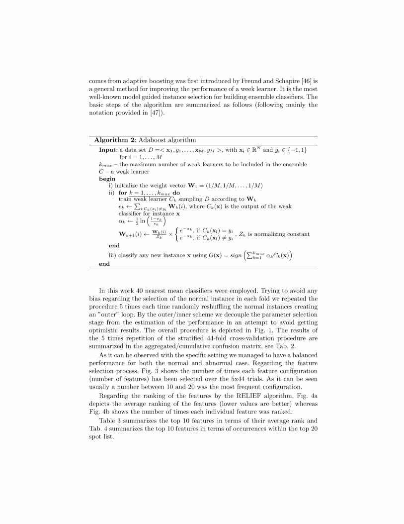
In this work 40 nearest mean classifiers were employed. Trying to avoid anybias regarding the selection of the normal instance in each fold we repeated theprocedure 5 times each time randomly reshuffling the normal instances creatingan ”outer” loop. By the outer/inner scheme we decouple the parameter selectionstage from the estimation of the performance in an attempt to avoid gettingoptimistic results. The overall procedure is depicted in Fig. 1. The results ofthe 5 times repetition of the stratified 44-fold cross-validation procedure aresummarized in the aggregated/cumulative confusion matrix, see Tab. 2.

As it can be observed with the specific setting we managed to have a balancedperformance for both the normal and abnormal case. Regarding the featureselection process, Fig. 3 shows the number of times each feature configuration(number of features) has been selected over the 5x44 trials. As it can be seenusually a number between 10 and 20 was the most frequent configuration.

Regarding the ranking of the features by the RELIEF algorithm, Fig. 4adepicts the average ranking of the features (lower values are better) whereasFig. 4b shows the number of times each individual feature was ranked.

Table 3 summarizes the top 10 features in terms of their average rank andTab. 4 summarizes the top 10 features in terms of occurrences within the top 20spot list.

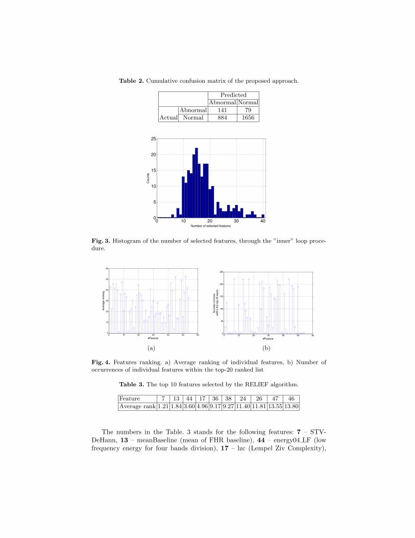
Table 2. Cumulative confusion matrix of the proposed approach.

PredictedAbnormal Normal

Abnormal 141 79Actual Normal 884 1656

Fig. 3. Histogram of the number of selected features, through the ”inner” loop proce-dure.

(a) (b)

Fig. 4. Features ranking. a) Average ranking of individual features, b) Number ofoccurrences of individual features within the top-20 ranked list

Table 3. The top 10 features selected by the RELIEF algorithm.

Feature 7 13 44 17 36 38 24 26 47 46

Average rank 1.21 1.84 3.60 4.96 9.17 9.27 11.40 11.81 13.55 13.80

The numbers in the Table. 3 stands for the following features: 7 – STV-DeHann, 13 – meanBaseline (mean of FHR baseline), 44 – energy04 LF (lowfrequency energy for four bands division), 17 – lzc (Lempel Ziv Complexity),

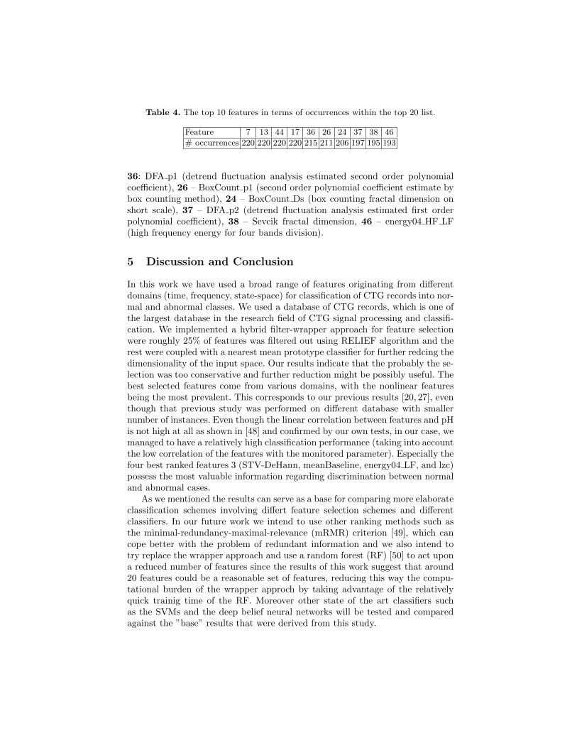
Table 4. The top 10 features in terms of occurrences within the top 20 list.

Feature 7 13 44 17 36 26 24 37 38 46

# occurrences 220 220 220 220 215 211 206 197 195 193

36: DFA p1 (detrend fluctuation analysis estimated second order polynomialcoefficient), 26 – BoxCount p1 (second order polynomial coefficient estimate bybox counting method), 24 – BoxCount Ds (box counting fractal dimension onshort scale), 37 – DFA p2 (detrend fluctuation analysis estimated first orderpolynomial coefficient), 38 – Sevcik fractal dimension, 46 – energy04 HF LF(high frequency energy for four bands division).

5 Discussion and Conclusion

In this work we have used a broad range of features originating from differentdomains (time, frequency, state-space) for classification of CTG records into nor-mal and abnormal classes. We used a database of CTG records, which is one ofthe largest database in the research field of CTG signal processing and classifi-cation. We implemented a hybrid filter-wrapper approach for feature selectionwere roughly 25% of features was filtered out using RELIEF algorithm and therest were coupled with a nearest mean prototype classifier for further redcing thedimensionality of the input space. Our results indicate that the probably the se-lection was too conservative and further reduction might be possibly useful. Thebest selected features come from various domains, with the nonlinear featuresbeing the most prevalent. This corresponds to our previous results [20, 27], eventhough that previous study was performed on different database with smallernumber of instances. Even though the linear correlation between features and pHis not high at all as shown in [48] and confirmed by our own tests, in our case, wemanaged to have a relatively high classification performance (taking into accountthe low correlation of the features with the monitored parameter). Especially thefour best ranked features 3 (STV-DeHann, meanBaseline, energy04 LF, and lzc)possess the most valuable information regarding discrimination between normaland abnormal cases.

As we mentioned the results can serve as a base for comparing more elaborateclassification schemes involving differt feature selection schemes and differentclassifiers. In our future work we intend to use other ranking methods such asthe minimal-redundancy-maximal-relevance (mRMR) criterion [49], which cancope better with the problem of redundant information and we also intend totry replace the wrapper approach and use a random forest (RF) [50] to act upona reduced number of features since the results of this work suggest that around20 features could be a reasonable set of features, reducing this way the compu-tational burden of the wrapper approch by taking advantage of the relativelyquick trainig time of the RF. Moreover other state of the art classifiers suchas the SVMs and the deep belief neural networks will be tested and comparedagainst the ”base” results that were derived from this study.

Acknowledgments

This work was supported by the following research programs: research grantNo.NT11124-6/2010 of the Ministry of Health Care of the Czech Republic,MSMT-11646/2012-36 of the Ministry of Education, Youth and Sports of theCzech Republic, CVUT grant SGS13/203/OHK3/3T/13, and by the joint re-search project ”Intelligent System for Automatic CardioTocoGraphic Data Anal-ysis and Evaluation using State of the Art Computational Intelligence Tech-niques” by the programme ”Greece-Czech Joint Research and Technology projects2011-2013”.

References

1. Alfirevic, Z., Devane, D., Gyte, G.M.L.: Continuous cardiotocography (CTG) asa form of electronic fetal monitoring (EFM) for fetal assessment during labour.Cochrane Database Syst Rev 3(3) (2006) CD006066

2. Bernardes, J., Costa-Pereira, A., de Campos, D.A., van Geijn, H.P., Pereira-Leite,L.: Evaluation of interobserver agreement of cardiotocograms. Int J GynaecolObstet 57(1) (Apr 1997) 33–37

3. Blix, E., Sviggum, O., Koss, K.S., Oian, P.: Inter-observer variation in assessmentof 845 labour admission tests: comparison between midwives and obstetricians inthe clinical setting and two experts. BJOG 110(1) (Jan 2003) 1–5

4. Chen, H.Y., Chauhan, S.P., Ananth, C.V., Vintzileos, A.M., Abuhamad, A.Z.:Electronic fetal heart rate monitoring and its relationship to neonatal and infantmortality in the United States. Am J Obstet Gynecol 204(6) (Jun 2011) 491.e1–491.10

5. Noren, H., Amer-Wahlin, I., Hagberg, H., Herbst, A., Kjellmer, I., Marsal, K.,Olofsson, P., Rosen, K.G.: Fetal electrocardiography in labor and neonatal out-come: data from the Swedish randomized controlled trial on intrapartum fetalmonitoring. Am J Obstet Gynecol 188(1) (Jan 2003) 183–192

6. Amer-Wahlin, I., Marsal, K.: ST analysis of fetal electrocardiography in labor.Seminars in Fetal and Neonatal Medicine 16(1) (2011) 29–35

7. FIGO: Guidelines for the Use of Fetal Monitoring. International Journal of Gyne-cology & Obstetrics 25 (1986) 159–167

8. ACOG: American College of Obstetricians and Gynecologists Practice BulletinNo. 106: Intrapartum fetal heart rate monitoring: nomenclature, interpretation,and general management principles. Obstet Gynecol 114(1) (Jul 2009) 192–202

9. Blackwell, S.C., Grobman, W.A., Antoniewicz, L., Hutchinson, M., Gyamfi Ban-nerman, C.: Interobserver and intraobserver reliability of the NICHD 3-Tier Fe-tal Heart Rate Interpretation System. Am J Obstet Gynecol 205(4) (Oct 2011)378.e1–378.e5

10. de Campos, D.A., Ugwumadu, A., Banfield, P., Lynch, P., Amin, P., Horwell, D.,Costa, A., Santos, C., Bernardes, J., Rosen, K.: A randomised clinical trial ofintrapartum fetal monitoring with computer analysis and alerts versus previouslyavailable monitoring. BMC Pregnancy Childbirth 10 (2010) 71

11. Dawes, G.S., Visser, G.H., Goodman, J.D., Redman, C.W.: Numerical analysisof the human fetal heart rate: the quality of ultrasound records. Am J ObstetGynecol 141(1) (Sep 1981) 43–52

12. de Campos, D.A., Sousa, P., Costa, A., Bernardes, J.: Omniview-SisPorto 3.5 -A central fetal monitoring station with online alerts based on computerized car-diotocogram+ST event analysis. Journal of Perinatal Medicine 36(3) (2008) 260–264

13. Task-Force: Heart rate variability. Standards of measurement, physiological inter-pretation, and clinical use. Task Force of the European Society of Cardiology andthe North American Society of Pacing and Electrophysiology. Eur Heart J 17(3)(Mar 1996) 354–381

14. Magenes, G., Signorini, M.G., Arduini, D.: Classification of cardiotocographicrecords by neural networks. In: Proc. IEEE-INNS-ENNS International Joint Con-ference on Neural Networks IJCNN 2000. Volume 3. (2000) 637–641

15. Goncalves, H., Rocha, A.P., de Campos, D.A., Bernardes, J.: Linear and nonlinearfetal heart rate analysis of normal and acidemic fetuses in the minutes precedingdelivery. Med Biol Eng Comput 44(10) (Oct 2006) 847–855

16. Van Laar, J., Porath, M., Peters, C., Oei, S.: Spectral analysis of fetal heartrate variability for fetal surveillance: Review of the literature. Acta Obstetricia etGynecologica Scandinavica 87(3) (2008) 300–306

17. Georgoulas, G., Stylios, C.D., Groumpos, P.P.: Feature Extraction and Classifica-tion of Fetal Heart Rate Using Wavelet Analysis and Support Vector Machines.International Journal on Artificial Intelligence Tools 15 (2005) 411–432

18. Ferrario, M., Signorini, M.G., Magenes, G., Cerutti, S.: Comparison of entropy-based regularity estimators: application to the fetal heart rate signal for the iden-tification of fetal distress. IEEE Trans Biomed Eng 53(1) (2006) 119–125

19. Goncalves, H., Bernardes, J., Rocha, A.P., de Campos, D.A.: Linear and nonlin-ear analysis of heart rate patterns associated with fetal behavioral states in theantepartum period. Early Hum Dev 83(9) (Sep 2007) 585–591

20. Spilka, J., Chudacek, V., Koucky, M., Lhotska, L., Huptych, M., Janku, P., Geor-goulas, G., Stylios, C.: Using nonlinear features for fetal heart rate classification.Biomedical Signal Processing and Control 7(4) (2012) 350–357

21. Georgoulas, G., Stylios, C.D., Groumpos, P.P.: Predicting the risk of metabolicacidosis for newborns based on fetal heart rate signal classification using supportvector machines. IEEE Trans Biomed Eng 53(5) (May 2006) 875–884

22. Czabanski, R., Jezewski, M., Wrobel, J., Jezewski, J., Horoba, K.: Predictingthe risk of low-fetal birth weight from cardiotocographic signals using ANBLIRsystem with deterministic annealing and epsilon-insensitive learning. IEEE TransInf Technol Biomed 14(4) (Jul 2010) 1062–1074

23. Georgieva, A., Payne, S.J., Moulden, M., Redman, C.W.G.: Artificial neural net-works applied to fetal monitoring in labour. Neural Computing and Applications22(1) (2013) 85–93

24. Georgoulas, G., Gavrilis, D., Tsoulos, I.G., Stylios, C.D., Bernardes, J., Groumpos,P.P.: Novel approach for fetal heart rate classification introducing grammaticalevolution. Biomedical Signal Processing and Control 2 (2007) 69–79

25. Sheiner, E., Hadar, A., Hallak, M., Katz, M., Mazor, M., Shoham-Vardi, I.: Clinicalsignificance of fetal heart rate tracings during the second stage of labor. ObstetGynecol 97(5 Pt 1) (May 2001) 747–752

26. Chudacek, V., Spilka, J., Bursa, M., Janku, P., Hruban, L., Huptych, M., Lhotska,L.: Open access intrapartum CTG database: Stepping stone towards generalizationof technical findings on CTG signals. PLoS ONE Manuscript submitted forpublication (2013)

27. Chudacek, V., Spilka, J., Lhotska, L., Janku, P., Koucky, M., Huptych, M., Bursa,M.: Assessment of features for automatic CTG analysis based on expert annotation.Conf Proc IEEE Eng Med Biol Soc 2011 (2011) 6051–6054

28. Cesarelli, M., Romano, M., Bifulco, P.: Comparison of short term variability in-dexes in cardiotocographic foetal monitoring. Comput Biol Med 39(2) (Feb 2009)106–118

29. de Haan, J., van Bemmel, J., Versteeg, B., Veth, A., Stolte, L., Janssens, J., Eskes,T.: Quantitative evaluation of fetal heart rate patterns. I. Processing methods.European Journal of Obstetrics and Gynecology and Reproductive Biology 1(3)(1971) 95–102 cited By (since 1996) 13.

30. Yeh, S.Y., Forsythe, A., Hon, E.H.: Quantification of fetal heart beat-to-beatinterval differences. Obstet Gynecol 41(3) (Mar 1973) 355–363

31. Pardey, J., Moulden, M., Redman, C.W.G.: A computer system for the numericalanalysis of nonstress tests. Am J Obstet Gynecol 186(5) (May 2002) 1095–1103

32. Signorini, M.G., Magenes, G., Cerutti, S., Arduini, D.: Linear and nonlinear param-eters for the analysis of fetal heart rate signal from cardiotocographic recordings.IEEE Trans Biomed Eng 50(3) (Mar 2003) 365–374

33. Higuchi, T.: Approach to an irregular time series on the basis of the fractal theory.Phys. D 31(2) (1988) 277–283

34. Kinsner, W.: Batch and real-time computation of a fractal dimension based onvariance of a time series. Technical report, Department of Electrical & ComputerEngineering, University of Manitoba, Winnipeg, Canada (1994)

35. Sevcik, C.: A Procedure to Estimate the Fractal Dimension of Waveforms. Com-plexity International 5 (1998) –

36. Peng, C.K., Havlin, S., Stanley, H.E., Goldberger, A.L.: Quantification of scalingexponents and crossover phenomena in nonstationary heartbeat time series. Chaos5(1) (1995) 82–87

37. Pincus, S.: Approximate entropy (ApEn) as a complexity measure. Chaos 5 (1)(1995) 110–117

38. Richman, J.S., Moorman, J.R.: Physiological time-series analysis using approxi-mate entropy and sample entropy. Am J Physiol Heart Circ Physiol 278(6) (Jun2000) H2039–H2049

39. Pincus, S.M., Viscarello, R.R.: Approximate entropy: a regularity measure for fetalheart rate analysis. Obstet Gynecol 79(2) (Feb 1992) 249–255

40. Lempel, A., Ziv, J.: On the complexity of finite sequences. IEEE Transactions onInformation Theory IT-22 (1) (1976) 75–81

41. Theodoridis, S., Koutroumbas, K.: Pattern recognition, 4th Edition (2009)

42. Guyon, I., Gunn, S., Nikravesh, M., Zadeh, L.A.: Feature extraction: foundationsand applications. Volume 207. Springer (2006)

43. Webb, A.R.: Statistical pattern recognition. Wiley (2003)

44. Chawla, N.V., Japkowicz, N., Kotcz, A.: Editorial: special issue on learning fromimbalanced data sets. ACM SIGKDD Explorations Newsletter 6(1) (2004) 1–6

45. Chawla, N.V., Bowyer, K.W., Hall, L.O., Kegelmeyer, W.P.: SMOTE: SyntheticMinority Over-sampling Technique. Journal of Artificial Intelligence Research 16(2002) 321–357

46. Freund, Y., Schapire, R.E.: Experiments with a New Boosting Algorithm. In:International Conference on Machine Learning. (1996) 148–156

47. Duda, R.O., Hart, P.E., Stork, D.G.: Pattern classification. New York: John Wiley,Section 10 (2001) l

48. Fulcher, B., Georgieva, A., Redman, C., Jones, N.: Highly comparative fetal heartrate analysis. In: Engineering in Medicine and Biology Society (EMBC), 2012Annual International Conference of the IEEE. (28 2012-sept. 1 2012) 3135 –3138

49. Peng, H., Long, F., Ding, C.: Feature selection based on mutual informationcriteria of max-dependency, max-relevance, and min-redundancy. Pattern Analysisand Machine Intelligence, IEEE Transactions on 27(8) (2005) 1226–1238

50. Breiman, L.: Random Forests. Machine Learning 45(1) (2001) 5–32