Embed Size (px)
Citation preview
ASYMPTOTICS FOR THE MULTIPLE POLE SOLUTIONS OF
THE NONLINEAR SCHRODINGER EQUATION
Cornelia Schiebold
Department of Natural Sciences, Engineering, and Mathematics
Mid Sweden University, S-851 70 Sundsvall, Sweden
Abstract. Multiple pole solutions consist of groups of weakly bound soli-
tons. For the Nonlinear Schrodinger equation the double pole solution wasconstructed by Zakharov and Shabat. In the sequel particular cases have been
discussed in the literature, but it has remained an open problem to understand
multiple pole solutions in their full complexity.In the present work this problem is solved, in the sense that a rigorous
and complete asymptotic description of the multiple pole solutions is given.
More precisely, the asymptotic paths of the solitons are determined and theirposition- and phase-shifts are computed explicitly. As a corollary we generalize
the conservation law known for the N -solitons. In the special case of one wave
packet, our result confirms a conjecture of Olmedilla.Our method stems from an operator theoretic approach to integrable sys-
tems. To facilitate comparison with the literature, we also establish the link tothe construction of multiple pole solutions via the Inverse Scattering Method.
The work is rounded off by many examples and Mathematica plots and a
detailed discussion of the transition to the next level of degeneracy.
Contents
1. Introduction 12. Construction of MPS’s 33. Main results on asymptotic behavior 64. Geometric interpretation and examples 95. Discussion of the assumptions 106. Link to ISM 147. Algebraic simplification of data 168. Collisions of wave packets 199. Collisions of the solitons within a wave packet 2510. Solutions of higher degeneracy 35Appendix A. Selected computer graphics 41Appendix B. Eigenvalue relations in the solution formula 41Appendix C. Global regularity 48References 50
1. Introduction
One of the most distinctive features of classical integrable systems like theKorteweg-de Vries equation (KdV) or the Nonlinear Schrodinger equation (NLS) isthe existence of N -solitons, i.e. solutions where N localized waves interact in elastic
1
2 CORNELIA SCHIEBOLD
collisions. Finding the formula for N -solitons (N ≥ 2) is nontrivial and was one ofthe motivations for the development of the Inverse Scattering Method (ISM), see[13], [2], [30]. In the framework of ISM, N -solitons are obtained in the reflection-less case if the transmission coefficient has N simple poles in the upper half plane.From an algebraic point of view, the next degree in complexity should correspondto multiple poles.
A priori it is not evident that this idea leads to new solutions. Actually thetransmission coefficient 1/a(k) of the eigenvalue equation (∂2
x−u(x))ψ = λψ (λ = k2)has only simple poles on the upper imaginary axis if the potentia u(x) belongs toL1(R) (see [11] for details). As a consequence one cannot obtain multiple polesolutions (MPS’s) of the KdV by applying the ISM in the usual way for functionsu(x, t) which are integrable w.r.t. x. On the other hand, it was early observed byZakharov and Shabat that multiple poles are possible for the NLS; in [30] theyconstruct solutions with a wave packet of two solitons by ‘coalescence’ of (twosimple) poles. From that time on, multiple pole solutions (MPS’s) for variousequations sporadically appear in the literature, see for example [12], [17], [27], [28],[29], mostly in cases of low complexity. A systematic study of the MPS’s of the NLSwas initiated by Olmedilla. In [15] he derives the formula for MPS’s with a singlewave packet consisting of L solitons by solving the Gelfand-Levitan-Marchenkoequation for the kernel corresponding to a single pole of order L at some pointk0 in the upper half plane (see Section 6 for details). Then he proceeds to anasymptotic analysis which finally reduces to the evaluation of a determinant whosecomplexity increases with L. The evaluation is only performed for L = 2 or 3. ForL ≤ 9, the author refers to computer computations and conjectures a formula for Larbitrary.
The main result of the present article is a complete and rigorous asymptoticanalysis of the MPS’s of the NLS
iqt = qxx + 2q∣q∣2. (1.1)
As a first major step towards this goal, we need formulas which nicely reflect thedecomposition into wave packets. Here we can build on an operator-theoretic ap-proach which can be trace back to Marchenko [14] and was subsequently amplifiedin the framework of advanced Banach space geometry ([4], [8], [23], [25], see [9]for an overview). There are numerous applications relying on analysis in infinitedimensional spaces [6], [7], [22], [25].
For our purposes, the main point is a solution formula depending on a matrixparameter whose Jordan form will give access to the asymptotic of the solution.The solution formula used here was first obtained in [21], see also [25]. For relatedwork we refer to [5], [10], [18]. Returning to a subtlety indicated above, we mentionthat formulas analogous to those used here give a natural access to the MPS’s ofthe KdV. In contrast to the NLS case, these contain pole-shaped antisolitons [9].
The asymptotic analysis is now performed on three levels of precision: First wewill show that MPS’s decompose into several wave packets situated in sectors in(x, t)-space. Second we examine the packets closer and discover that each of themdecomposes into finitely many solitons which logarithmically drift away from a com-mon geometric center, which itself moves with constant velocity. As in the familiarcase of N -solitons, the collision of various entities (transition from asymptotics fort → −∞ to t → ∞) is described by position- and phase-shifts, which are explicitlycomputed in the third step. This computation turns out to be considerably more
3
involved as for other equations ([19], [20]). Fortunately we can massively rely onour earlier results published in [24]. For one single wave packet, our result confirmsthe conjecture of Olmedilla.
The article is organizes as follows. After constructing determinant formulas forMPS’s in Section 2, we formulate our main results on their asymptotic behaviorin Section 3. Section 4 explains the underlying geometry, followed by some plotsindicating the subtle interaction behavior of MPS’s. Section 5 addresses the as-sumptions in the central Theorem 3.3. First we point out why the various technicalassumptions do not restrict generality. A crucial further assumption specifies thetransition to the next level of degeneracy. This happens if there are solitons or wavepackets with the same velocity but corresponding to different poles. We discuss thesimplest example for this phenomenon. As mentioned above, Olmedilla’s point ofdeparture is the ISM. In Section 6 we establish the link between the two approachesand show in particular that all solutions constructed in [15] are covered by Theorem3.3. After a parameter reduction in Section 7, the proof of Theorem 3.3 is givenin Sections 8 and 9. In Section 10 we return to solutions of higher degeneracy andsketch in the first relevant case which of their properties can be captured by asymp-totic analysis. The article is concluded by three appendices with complementingmaterial. Appendix A presents some computer plots of more complicated MPS’s.In Appendix B we verify an invariance property for the eigenvalues. In AppendixC we give a rigorous proof that all solutions in Theorem 2.3 (including those ofhigher degeneracy) are globally regular.
Acknowledgement. Section 6 owes much to enlightening discussions with TuncayAktosun about the ISM.
2. Construction of MPS’s
First we explain the construction of MPS’s as used in the present work. We startwith an analogue of the 1-soliton for the matrix-Nonlinear Schrodinger equation(matrix-NLS)
iQt = Qxx + 2QQQ. (2.1)
Here the unknown Q = Q(x, t) is a function with values in the n × n-matrices, and
Q denotes the matrix obtained from Q by taking complex conjugated entries.As a close variant, the equation (2.1) with Q replaced by Q∗, the adjoint of Q,
is often considered in the literature (see [1], [5], [10] and references therein). Forour needs the two approaches are essentially equivalent since we mainly use themto derive handy solution formulas.
Proposition 2.1. Let A,C ∈ Mn,n(C), and define L(x, t) = exp(Ax − iA2t)C =eAx−iA2tC. Then
Q = (I +LL)−1(AL +LA), (2.2)
where I denotes the identity matrix, is a solution of the matrix-NLS (2.1) on
(x, t) ∈ R2 ∣ I +LL invertible.
Proposition 2.1 is a special case of more general solution formulas for the operator-NLS [22], see also [23] for the operator-AKNS system. For the reader’s convenience,we give a direct proof.
4 CORNELIA SCHIEBOLD
Proof. Using Lt = −iA2L (and thus Lt = iA2L), we calculate
Qt = −(I +LL)−1 ( LL )t(I +LL)−1(AL +LA) + (I +LL)−1 ( AL +LA )
t
= i(I +LL)−1 ( A2L −LA2 ) L(I +LL)−1(AL +LA)−i(I +LL)−1A2 ( AL +LA )
= i(I +LL)−1 ( (A2L −LA2)L −A2(I +LL) ) (I +LL)−1(AL +LA)
= −i(I +LL)−1(A2 +LA2L)Q.
Similarly, one obtains Qx = QQ.Using L(I + LL)−1 = (I + LL)−1L, L(I + LL)−1L = I − (I + LL)−1, (I + LL)−1 =
I −L(I +LL)−1L, and (I +LL)−1L = L(I +LL)−1, we get
QQ = (I +LL)−1((AL +LA)(I +LL)−1(AL +LA))
= (I +LL)−1(A ( L(I +LL)−1 ) AL +A ( L(I +LL)−1L ) A
+LA ( (I +LL)−1 ) AL +LA ( (I +LL)−1L ) A)
= (I +LL)−1(A ( (I +LL)−1L ) AL +A ( I − (I +LL)−1 ) A
+LA ( I −L(I +LL)−1L ) AL +LA ( L(I +LL)−1 ) A)
= (I +LL)−1(A2 +LA2L) − (I +LL)−1(A −LAL)(I +LL)−1(A −LAL)
= (I +LL)−1(A2 +LA2L) − Q2, (2.3)
where Q = (I + LL)−1(A − LAL). Moreover, Qx = −QQ. Thus we get Qxx =(QQ)x = −QQQ + Q2Q, and therefore
Qxx + 2QQQ = (Q2 +QQ)Q (2.3)= (I +LL)−1(A2 +LA2L)Q = iQt.
The solution (2.2) is a matrix generalization of the well-known 1-soliton. In fact,setting n = 1 and A = α, C = exp(ϕ), we get L(x, t) = `(x, t) = exp(αx − iα2t + ϕ)and
q(x, t) = 2Re(α) `(x, t)1 + ∣`(x, t)∣2
= Re(α) ei Im(Γ(x, t)) cosh−1 (Re(Γ(x, t))),
where Γ(x, t) = αx− iα2t+ϕ. Note that Re(Γ) = Re(α)(x+2Im(α)t)+Re(ϕ). Thus∣Re(α)∣ is the height of the soliton and v = −2Im(α) its velocity. Since height andvelocity can be specified independently, we may have superpositions of solitons withthe same velocity but different heights, see also Example 5.1 and the discussion inSection 10.
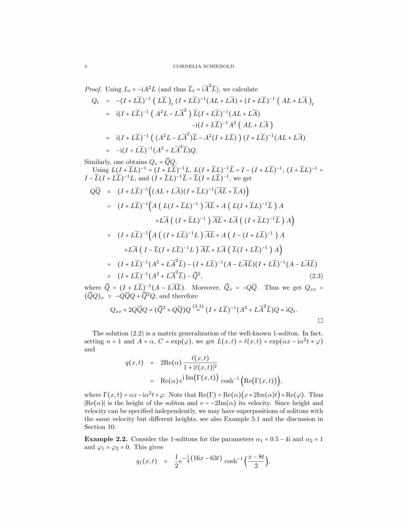
Example 2.2. Consider the 1-solitons for the parameters α1 = 0.5 − 4i and α2 = 1and ϕ1 = ϕ2 = 0. This gives
q1(x, t) = 1
2e−
i4(16x − 63t) cosh−1 (x − 8t
2),
5
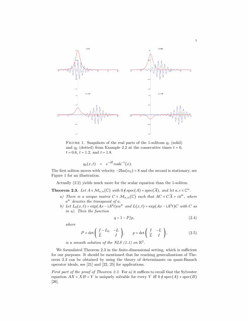
Figure 1. Snapshots of the real parts of the 1-solitons q1 (solid)and q2 (dotted) from Example 2.2 at the consecutive times t = 0,t = 0.6, t = 1.2, and t = 1.8.
q2(x, t) = e−it cosh−1(x).The first soliton moves with velocity −2Im(α2) = 8 and the second is stationary, seeFigure 1 for an illustration.
Actually (2.2) yields much more for the scalar equation than the 1-soliton.
Theorem 2.3. Let A ∈Mn,n(C) with 0 /∈ spec(A) + spec(A), and let a, c ∈ Cn.
a) There is a unique matrix C ∈Mn,n(C) such that AC + CA = catr , whereatr denotes the transposed of a.
b) Let L0(x, t) = exp(Ax − iA2t)catr and L(x, t) = exp(Ax − iA2t)C with C asin a). Then the function
q = 1 − P /p, (2.4)
where
P = det( I −L0 −LL I
) , p = det( I −LL I
) , (2.5)
is a smooth solution of the NLS (1.1) on R2.
We formulated Theorem 2.3 in the finite-dimensional setting, which is sufficientfor our purposes. It should be mentioned that far reaching generalizations of The-orem 2.3 can be obtained by using the theory of determinants on quasi-Banachoperator ideals, see [21] and [22, 25] for applications.
First part of the proof of Theorem 2.3. For a) it suffices to recall that the Sylvesterequation AX +XB = Y is uniquely solvable for every Y iff 0 /∈ spec(A) + spec(B)[26].
6 CORNELIA SCHIEBOLD
Here we prove b) only on the set Ω = (x, t) ∣ I + LL invertible and postponethe proof that Ω = R2 to Appendix C. To this end, we first show that the scalarfunction
q = atr(I +LL)−1Fc, (2.6)
where F = F (x, t) = exp(Ax − iA2t), is a solution of (1.1). Applying Proposition2.1, we find that
Q = (I +LL)−1Fcatr
solves the matrix-NLS (2.1). Abbreviating Q0 = (I +LL)−1F , this means that
iQ0,tcatr = Q0,xxca
tr + 2Q0catr Q0ca
tr Q0catr .
We may assume a /= 0. Choosing some vector d with atrd = 1 and multiplying theabove matrix equation with d from the right, and with atr from the left, we obtain
iqt = i(atrQ0c)t= iatrQ0,tc
= atrQ0,xxc + 2 atr Q0catr Q0ca
tr Q0c
= (atrQ0c)xx + 2(atrQ0c)(atrQ0c)(atrQ0c)= qxx + 2q∣q∣2.
Next we rewrite (2.6) in the form (2.4), (2.5). We start by observing that
q = atrQ0c = tr ( Q0catr ) = 1 − det ( I −Q0ca
tr ),
where we have used the fact that det(I + A) = 1 + tr(A) holds for every rank-1
matrix A. Recall Q0 = (I +LL)−1F and Fcatr = L0. For (x, t) ∈ Ω, this gives
q = 1 − det ( I − (I +LL)−1L0 )= 1 − det ( (I +LL)−1(I +LL −L0) )
= 1 − det(I +LL −L0)det(I +LL)
.
From this, the desired form of the solution is obtained by using
det( A B1
B2 I) = det (( A B1
B2 I)( I 0
−B2 I)) = det( A −B1B2 B1
0 I)
= det ( A −B1B2 ), (2.7)
which holds for every square matrix A.
3. Main results on asymptotic behavior
Now we turn to the asymptotics of the solutions provided by Theorem 2.3.We say that two functions f = f(x, t), g = g(x, t) have the same asymptotic
behavior for t → ∞ (t → −∞) if for every ε > 0 there is a tε such that ∣f(x, t) −g(x, t)∣ < ε for t > tε (t < tε) and x ∈ R. In this case we also write f(x, t) ≈g(x, t) for t ≈∞ (t ≈ −∞).
We will formulate further assumptions, one essential for an asymptotic exami-nation, the others with the mere purpose to simplify notation. Let us start withtwo assumptions of the second type.

7
Assumption 3.1. The matrix A ∈ Mn,n(C) is in Jordan form with N Jordanblocks Aj of size nj × nj corresponding to the eigenvalues αj, i.e.,
A =⎛⎜⎜⎜⎝
A1 0 ⋯ 00 A2 ⋯ 0. . . . . . . . . . . . . . . . .0 0 ⋯ AN
⎞⎟⎟⎟⎠, Aj =
⎛⎜⎝
αj 1 0⋅ ⋅⋅ ⋅⋅ 1
0 αj
⎞⎟⎠∈Mnj ,nj(C).
It is useful to adapt our notation to the given Jordan structure of A: For a vectorc ∈ Cn, we write
c = (cj)Nj=1 with cj = (c(µ)j )njµ=1 ∈ Cnj ,
and, analogously, for a matrix T ∈Mn,n(C),
T = (Tij)Nij=1 with Tij = (t(µν)ij ) µ=1,...,niν=1,...,nj
∈Mni,nj(C).
Assumption 3.2. The vectors a, c ∈ Cn satisfy a(1)j c
(nj)j /= 0.
In Section 5 it is shown that Assumptions 3.1 and 3.2 can be made without lossof generality. Now we are in position to state our main result.
Theorem 3.3. Let Assumptions 3.1 and 3.2 be met and suppose that
a) the Re(αj) are positive,b) the Im(αj) are pairwise different.
To these data we associate the (soliton-like) functions
q±jj′(x, t) = sgn(t)nj−1 Re(αj)ei Im(Γ±jj′(x, t)) cosh−1 (Re(Γ±jj′(x, t)))
for j′ = 0, . . . , nj − 1 with
Γ±jj′(x, t) = αjx − iα2j t ∓ J ′ log ∣t∣ + ϕj + ϕ±j + ϕ±jj′ ,
where we have set J ′ = −(nj − 1) + 2j′. The quantities ϕj, ϕ±j are (up to integer
multiples of 2πi) defined by
exp(ϕj) = ia(1)j c
(nj)j /(2iRe(αj))nj , (3.1)
exp(ϕ±j ) = ∏k∈Λ±
j
[αj − αkαj + αk
]2nk
(3.2)
with the index sets Λ±j = k ∣ Im(αj) ≶ Im(αk), and the quantities ϕ±jj′ are defined
by
ϕ±jj′ = ± log (( 2Re(αj) )−2J ′ j′!
(j′ − J ′)! ) . (3.3)
Then the asymptotic behavior of the solution q(x, t) associated to the data A, a, cby Theorem 2.3 is
q(x, t) ≈N
∑j=1
nj−1
∑j′=0
q±jj′(x, t) for t ≈ ±∞.
8 CORNELIA SCHIEBOLD
The above theorem says that the solitons q±jj′(x, t) travel asymptotically along
the logarithmic curves (x, t) ∈ R2 ∣ Re(Γ±jj′(x, t)) = 0, i.e. the velocity of q±jj′(x, t)is vj = −2Im(αj), up to a logarithmic deviation. Hence, for j′ = 0, . . . , nj − 1 theq±jj′(x, t) can be viewed as a weakly bound group or wave packet. Their oscillation
is encoded by Im(Γ±jj′(x, t)).The initial shift ϕj determines position and phase of the geometric center of
the jth wave packet at a given time. Note that it is a parameter of the solution.The quantities ϕ±j encode position- and phase-shifts in the asymptotic form due tocollisions of wave packets with different velocities. Here the index sets Λ+
j (resp. Λ−j )
stand for those wave packets which move slower (resp. faster) than the jth wavepacket. The ϕ±jj′ encode the positioning of the solitons within the jth wave packet.
Observe that the wave corresponding to j′ = 0 moves the furthest to the left fort ≈ −∞ and the furthest to the right for t ≈∞. This suggests that the solitons flipside during collision, a phenomenon which becomes more transparent for MPS’sof the KdV. Here a packet with two waves comprises a soliton and an antisoliton(with a polar singularity) and their changing of side is manifest [9].
A detailed discussion of the assumptions is postponed to Section 5. Here we justobserve that the main purpose of a) is to simplify formulas. Actually Re(αj) /= 0is enough, see Section 5. In contrast b) is essential, since it ensures that the wavepackets travel with different velocities. However, in Sections 4 and 10 we will lookat examples with eigenvalues α1 /= α2 satisfying Im(α1) = Im(α2). Our observationssuggest a study of such solutions in coarser terms.
For several reasons it is not straightforward to verify that our formulas includethose of [15, 30]. The details are provided in Remark 9.8.
By a direct calculation, we deduce the following conservation law from (3.2).
Corollary 3.4. The sum of all position-shifts vanishes:
N
∑j=1
nj ( Re(ϕ+j ) −Re(ϕ−j ) ) = 0.
Proof. Without loss of generality, Im(α1) < . . . < Im(αN). Then Λ−j = 1, . . . , j −1,
Λ+j = j + 1, . . . ,N, and
ϕ ∶=N
∑j=1
nj ( ϕ+j − ϕ−j ) = 2N
∑j=1
N
∑k=j+1
njnk logAjk − 2N
∑j=1
j−1
∑k=1
njnk logAjk
= 2N
∑j=1
N
∑k=j+1
njnk logAjk − 2N
∑k=1
N
∑j=k+1
njnk logAjk
= 2N
∑j=1
N
∑k=j+1
njnk logAjk
Akj
for Ajk = (αj − αkαj + αk
)2
. SinceAjk
Akj= (αj + αk
αj + αk)
2
has modulus 1, it follows ϕ ∈ iR.
Remark 3.5. It is worth mentioning that the ϕ±jj′ satisfy the following symmetryproperty which concerns the positioning of pairs of solitons which are approximatelyrelated by reflection in the geometric center of the jth wave packet:
∀j′ ∶ ϕ±jj′ = −ϕ±j(nj−1−j′).
9
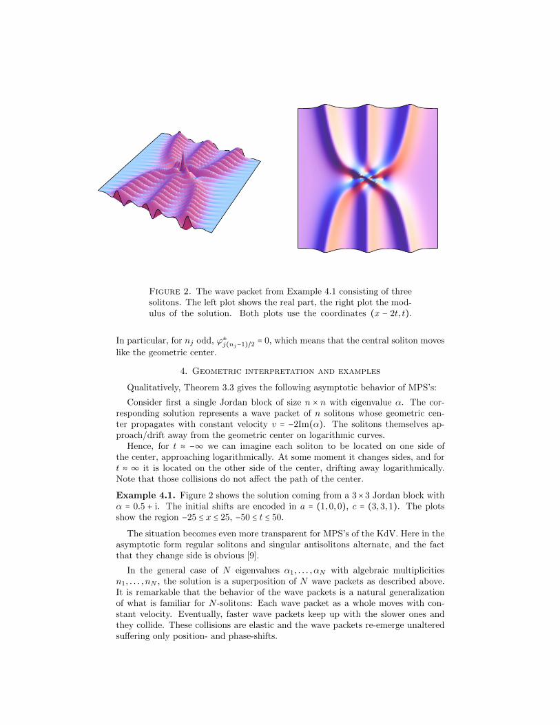
Figure 2. The wave packet from Example 4.1 consisting of threesolitons. The left plot shows the real part, the right plot the mod-ulus of the solution. Both plots use the coordinates (x − 2t, t).
In particular, for nj odd, ϕ±j(nj−1)/2 = 0, which means that the central soliton moves
like the geometric center.
4. Geometric interpretation and examples
Qualitatively, Theorem 3.3 gives the following asymptotic behavior of MPS’s:
Consider first a single Jordan block of size n × n with eigenvalue α. The cor-responding solution represents a wave packet of n solitons whose geometric cen-ter propagates with constant velocity v = −2Im(α). The solitons themselves ap-proach/drift away from the geometric center on logarithmic curves.
Hence, for t ≈ −∞ we can imagine each soliton to be located on one side ofthe center, approaching logarithmically. At some moment it changes sides, and fort ≈ ∞ it is located on the other side of the center, drifting away logarithmically.Note that those collisions do not affect the path of the center.
Example 4.1. Figure 2 shows the solution coming from a 3× 3 Jordan block withα = 0.5 + i. The initial shifts are encoded in a = (1,0,0), c = (3,3,1). The plotsshow the region −25 ≤ x ≤ 25, −50 ≤ t ≤ 50.
The situation becomes even more transparent for MPS’s of the KdV. Here in theasymptotic form regular solitons and singular antisolitons alternate, and the factthat they change side is obvious [9].
In the general case of N eigenvalues α1, . . . , αN with algebraic multiplicitiesn1, . . . , nN , the solution is a superposition of N wave packets as described above.It is remarkable that the behavior of the wave packets is a natural generalizationof what is familiar for N -solitons: Each wave packet as a whole moves with con-stant velocity. Eventually, faster wave packets keep up with the slower ones andthey collide. These collisions are elastic and the wave packets re-emerge unalteredsuffering only position- and phase-shifts.
10 CORNELIA SCHIEBOLD
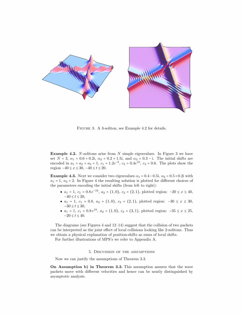
Figure 3. A 3-soliton, see Example 4.2 for details.
Example 4.2. N -solitons arise from N simple eigenvalues. In Figure 3 we haveset N = 3, α1 = 0.6 + 0.2i, α2 = 0.2 + 1.5i, and α3 = 0.3 − i. The initial shifts areencoded in a1 = a2 = a3 = 1, c1 = 1.2e−2, c2 = 0.4e10, c3 = 0.6. The plots show theregion −40 ≤ x ≤ 30, −40 ≤ t ≤ 20.
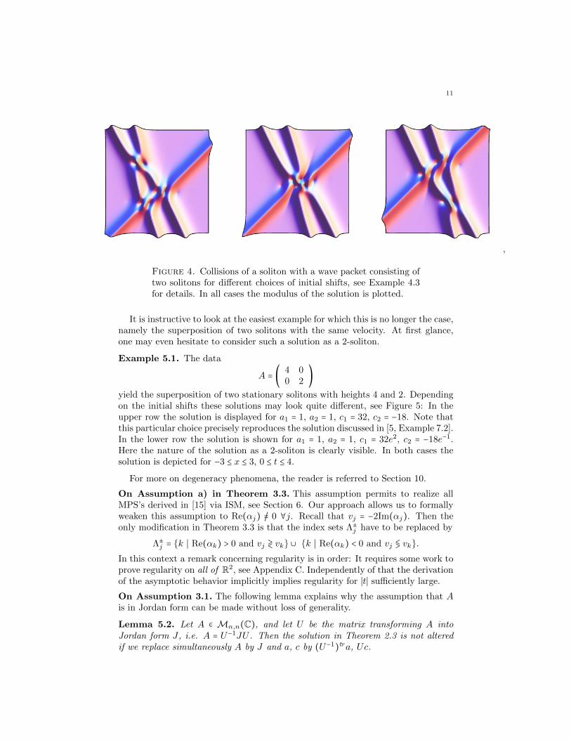
Example 4.3. Next we consider two eigenvalues α1 = 0.4−0.5i, α2 = 0.5+0.2i withn1 = 1, n2 = 2. In Figure 4 the resulting solution is plotted for different choices ofthe parameters encoding the initial shifts (from left to right):
a1 = 1, c1 = 0.8 e−10, a2 = (1,0), c2 = (2,1), plotted region: −20 ≤ x ≤ 40,−40 ≤ t ≤ 20,
a1 = 1, c1 = 0.8, a2 = (1,0), c2 = (2,1), plotted region: −30 ≤ x ≤ 30,−30 ≤ t ≤ 30,
a1 = 1, c1 = 0.8 e10, a2 = (1,0), c2 = (3,1), plotted region: −35 ≤ x ≤ 25,−20 ≤ t ≤ 40.
The diagrams (see Figures 4 and 12–14) suggest that the collision of two packetscan be interpreted as the joint effect of local collisions looking like 2-solitons. Thuswe obtain a physical explanation of position-shifts as sums of local shifts.
For further illustrations of MPS’s we refer to Appendix A.
5. Discussion of the assumptions
Now we can justify the assumptions of Theorem 3.3.
On Assumption b) in Theorem 3.3. This assumption assures that the wavepackets move with different velocities and hence can be neatly distinguished byasymptotic analysis.
11
,
Figure 4. Collisions of a soliton with a wave packet consisting oftwo solitons for different choices of initial shifts, see Example 4.3for details. In all cases the modulus of the solution is plotted.
It is instructive to look at the easiest example for which this is no longer the case,namely the superposition of two solitons with the same velocity. At first glance,one may even hesitate to consider such a solution as a 2-soliton.
Example 5.1. The data
A = ( 4 00 2
)
yield the superposition of two stationary solitons with heights 4 and 2. Dependingon the initial shifts these solutions may look quite different, see Figure 5: In theupper row the solution is displayed for a1 = 1, a2 = 1, c1 = 32, c2 = −18. Note thatthis particular choice precisely reproduces the solution discussed in [5, Example 7.2].In the lower row the solution is shown for a1 = 1, a2 = 1, c1 = 32e2, c2 = −18e−1.Here the nature of the solution as a 2-soliton is clearly visible. In both cases thesolution is depicted for −3 ≤ x ≤ 3, 0 ≤ t ≤ 4.
For more on degeneracy phenomena, the reader is referred to Section 10.
On Assumption a) in Theorem 3.3. This assumption permits to realize allMPS’s derived in [15] via ISM, see Section 6. Our approach allows us to formallyweaken this assumption to Re(αj) /= 0 ∀j. Recall that vj = −2Im(αj). Then theonly modification in Theorem 3.3 is that the index sets Λ±
j have to be replaced by
Λ±j = k ∣ Re(αk) > 0 and vj ≷ vk ∪ k ∣ Re(αk) < 0 and vj ≶ vk.
In this context a remark concerning regularity is in order: It requires some work toprove regularity on all of R2, see Appendix C. Independently of that the derivationof the asymptotic behavior implicitly implies regularity for ∣t∣ sufficiently large.
On Assumption 3.1. The following lemma explains why the assumption that Ais in Jordan form can be made without loss of generality.
Lemma 5.2. Let A ∈ Mn,n(C), and let U be the matrix transforming A intoJordan form J , i.e. A = U−1JU . Then the solution in Theorem 2.3 is not alteredif we replace simultaneously A by J and a, c by (U−1)tra, Uc.

12 CORNELIA SCHIEBOLD
Figure 5. Two stationary solitons with different choices of initialposition-shifts, see Example 5.1 for details. In the upper plotsboth solitons have approximately the same geometric center. Inthe lower plots this is no longer the case, and the solitons are wellseparated. To the left the respective real part, to the right themodulus is plotted.
Proof. Let b = (U tr)−1a, d = Uc, and D = UCU −1. First we observe that, replacing
A by J and a, c by b, d implies replacing C, the (unique) solution of the Sylvester
equation AX +XA = catr , by D. Indeed, since
dbtr = (Uc)((U −1)tra)tr = U(catr)U −1 = U(AC +CA)U −1
= U(U−1JUC +CU −1JU)U −1 = JUCU
−1 +UCU −1J = JD +DJ,
D satisfies JD +DJ = dbtr . Moreover, from the very definition of the exponentialfunction,
exp(Ax − iA2t) = U−1 exp(Jx − iJ2t)U.
13
Abbreviating K = exp(Jx − iJ2t)D and K0 = exp(Jx − iJ2t)dbtr , we thus have
L = exp(Ax − iA2t)C = U−1 exp(Jx − iJ2t)U (U−1DU) = U−1KU,
L0 = exp(Ax − iA2t)(catr) = U−1 exp(Jx − iJ2t)U ((U−1d)(U trb)tr) = U−1K0U,
yielding
P = det ( I + ( −L0 −LL 0
) )
= det ( I + (U−1 0
0 U−1 )( −K0 −K
K 0)( U 0
0 U) )
= det ( I + ( −K0 −KK 0
) ),
showing that the replacements do not change the determinant P . A similar, eveneasier calculation allows to handle p.
On Assumption 3.2. At first glance this assumption on the vectors a, c (namely
a(1)j c
(nj)j /= 0 ∀j) looks artificial. However, the following lemma shows that it can
indeed be made without losing anything.
Lemma 5.3. Let Assumption 3.1 be met and a, c ∈ Cn/0 satisfy c(nk)k = 0 or
a(1)k = 0. Then the solution given in Theorem 2.3 is not altered if we replace simul-
taneously A by A, and a, c by a, c, where
a) A is the matrix obtained from A by reducing the size of the Jordan blockAk by one, more precisely by omitting in A the row/column which containsthe last row/column of Ak,
b) a, c are the vectors obtained from a, c by deleting the entries
a(nk)k , c
(nk)k for c
(nk)k = 0,
a(1)k , c
(1)k for a
(1)k = 0.
Proof. We treat the case c(nk)k = 0, the other being symmetric.
Set d(x, t) = exp(Ax − iA2t)c. Note that L0(x, t) = d(x, t)atr , and that L(x, t)is the unique matrix satisfying the (x, t)-dependent Sylvester equation AX(x, t) +X(x, t)A = d(x, t)atr .
Since A is a block diagonal matrix with upper triangular matrices on the di-agonal, the same holds for exp(Ax − iA2t). More precisely, exp(Ax − iA2t) =diagexp(Ajx − iA2
j t) ∣ j = 1, . . . ,N and hence d(x, t) = (dj(x, t))j with dj(x, t) =exp(Ajx − iA2
j t)cj .Since exp(Akx − iA2
kt) is upper triangular, c(nk)k = 0 implies d
(nk)k = 0, and we
havedk(x, t) = ( exp(Akx − iA2
kt)ck,0 ),where Ak is the block obtained from Ak by reducing the dimension by one andck the vector obtained from ck by deleting the nkth entry. Consequently L0 =d(x, t)atr = (di(x, t)atrj )N
i,j=1has a zero-row, namely the (n1 + . . . + nk)th row.
The fact that the same holds for L can be seen from the factorization of thesolution of the Sylvester equation given in Lemma 7.3. Now the assertion followsfrom expanding the determinants P , p.

14 CORNELIA SCHIEBOLD
Remark 5.4. In the case nk = 1 the above procedure amounts to crossing out Ak,ak, ck completely. If there is only one block left, this leads to the trivial solution.
6. Link to ISM
In this section we establish the link to Olmedilla’a derivation [15] of MPS’s viaISM. This construction starts out from the data of principal parts
rj(k) =rjnj
(k − kj)nj+
rjnj−1
(k − kj)nj−1+ . . . + rj1
k − kj(6.1)
given at N points k1, . . . , kN in the upper half plane H = Im(k) > 0. Following[15], we associate to (6.1) the kernel
Ω(z; t) = −2iN
∑j=1
resk=kj(rj(k)e2ikz−4ik2t). (6.2)
The main goal of this section is to solve the corresponding Gelfand-Levitan-Marchenko(GLM) equation
K(x, y; t)+∫∞
0∫
∞
0K(x, s; t)Ω(x+s+z; t)Ω(x + y + z; t) ds dz = Ω(x + y; t). (6.3)
Step 1: Rewriting the kernel. Since the function `(k) = e2ikz−4ik2t is holomor-phic, its Taylor expansion together with (6.1) give
resk=kj(rj(k)`(k)) =nj
∑ν=1
rjν
(ν − 1)!∂ν−1`
∂kν−1(kj)
= (`1(kj), . . . , `nj(kj))dj ,
where we have set `ν(k) =1
(ν − 1)!∂ν−1`
∂kν−1(k) and dj =
⎛⎜⎝
rj1⋮
rjnj
⎞⎟⎠
.
Let Λj = 2iJj , where Jj is the nj × nj-Jordan block corresponding to the eigen-value kj . By Lemma 7.2,
eΛjz+iΛ2j t =
⎛⎜⎝
`1(kj) `nj(kj)⋱
0 `1(kj)
⎞⎟⎠.
Multiplying with the transposed of the first standard basis vector e(1)nj in Cnj from
the left gives us the first row of this matrix. Thus we find
resk=kj(rj(k)`(k)) = (e(1)nj )treΛjz+iΛ2
j t dj .
Let now Λ = diagΛ1, . . . ,ΛN be the block diagonal matrix with the nj ×nj-blocksΛj on the diagonal. Then
eΛz+iΛ2t = diageΛjz+iΛ2j t ∣ j = 1, . . . ,N,
and henceN
∑j=1
resk=kj(rj(k)`(k)) =N
∑j=1
(e(1)nj )treΛjz+iΛ2
j t dj
= f treΛz+iΛ2td

15
for the vectors f = (e(1)nj )Nj=1 and d = (dj)Nj=1. Hence the kernel (6.2) can be writtenin the form
Ω(z; t) = −2if tr eΛz+iΛ2t d. (6.4)
Observe that the spectrum of the matrix Λ is contained in the left complex half-plane.
Step 2: Solving the GLM equation. Let D be the unique solution of the
Sylvester equation ΛX +XΛ = −2idf tr and set G(x, t) = eΛx+iΛ2tD. In this step weshow that
K(x, y; t) = 2if tr(I +G(x, t) G(x, t))−1eΛ(x+y)−iΛ
2t d (6.5)
solves the GLM equation (6.3) with kernel (6.4) (see Appendix C for the invertibility
of I +G(x, t)G(x, t) on R2).To this end, we first observe that
2i∫∞
0eΛs df treΛs ds = −∫
∞
0eΛs(ΛD +DΛ)eΛs ds = −∫
∞
0
d
ds(eΛsDeΛs) ds =D,
where we have used that the spectra of Λ, Λ are contained in the left complexhalf-plane. Since f has real entries, we also have
− 2i∫∞
0eΛs df treΛs ds =D. (6.6)
Abbreviating M(x, t) = (I +G(x, t)G(x, t))−1, we get
∫∞
0K(x, s; t)Ω(x + s + z; t) ds
= −(2i)2 ∫∞
0(f trM(x, t)eΛ(x+s)−iΛ
2t d) (f treΛ(x+s+z)+iΛ2t d) ds
= 2if trM(x, t) ( − 2i eΛx−iΛ2t ∫
∞
0eΛs df treΛs ds) eΛ(x+z)+iΛ2td
(6.6)= 2if trM(x, t) G(x, t) eΛ(x+z)+iΛ2td.
Now we can verify (6.3):
∫∞
0∫
∞
0K(x, s; t)Ω(x + s + z; t)Ω(x + y + z; t) ds dz
= (2i)2 ∫∞
0(f trM(x, t)G(x, t)eΛ(x+z)+iΛ2t d) (f treΛ(x+z+y)−iΛ
2td) dz
= 2if trM(x, t)G(x, t) ( 2i eΛx+iΛ2t ∫∞
0eΛzdf treΛz dz) eΛ(x+y)−iΛ
2td
= 2if tr (M(x, t)G(x, t)G(x, t) ) eΛ(x+y)−iΛ2td
= 2if tr ( I −M(x, t) ) eΛ(x+y)−iΛ2td
= Ω(x + y; t) −K(x, y; t).
Step 3: Conclusions. From the formalism of the ISM, the corresponding potentialq is obtained via
q(x, t) = −K(x,0; t)
= −2if tr ( I +G(x, t)G(x, t) )−1eΛx−iΛ
2td.
16 CORNELIA SCHIEBOLD
Using the trace representation (2.6), it is easy to check that these potentials areincluded in the solution class of Theorem 2.3 for
A = Λ, a = −2if, c = d.
Let us summarize: The MPS’s considered in [15] are derived as solutions of (6.3)with kernels as in (6.2). In all these cases we have solved (6.3) by functions K whoseassociated potentials are included in the solution class of Theorem 2.3. Because ofknown uniqueness properties of the GLM equation (see [3, page 24]), the results in[15] on asymptotic behavior of MPS’s (only MPS’s consisting of one wave packetwith at most three waves are treated in [15]) are special cases of Theorem 3.3. Notealso that the above reasoning complements the derivation of explicit expressionsfor solutions in [15], where the GLM equation is only solved for N = 1.
7. Algebraic simplification of data
In the following proposition MPS’s are rewritten in a form suitable for asymptoticanalysis.
Proposition 7.1. The determinants P , p in the formula of the solution given inTheorem 2.3 can be expressed as
p(x, t) = det (I + ( M 0
0 M)( 0 −T
T 0)),
P (x, t) = det (I + ( M 0
0 M)( −ff tr −T
T 0)),
where
a) T = (Tij)N
i,j=1with
Tij =⎛⎝(−1)µ+ν(µ + ν − 2
µ − 1)( 1
αi + αj)µ+ν−1⎞
⎠ µ=1,...,niν=1,...,nj
,
b) f ∈ Cn denotes the vector f = (e(1)nj )N
j=1consisting of the first standard basis
vectors e(1)nj ∈ Cnj for j = 1, . . . ,N , and
c) M = diagMj ∣ j = 1, . . . ,N with
Mj =⎛⎜⎝
m(1)j m
(nj)j⋰
m(nj)j 0
⎞⎟⎠∈Mnj ,nj(C),
the entries given by
m(µ)j = m
(µ)j (x, t) =
nj−(µ−1)
∑κ=1
b(µ−1+κ)j
1
(κ − 1)!∂κ−1
∂ακ−1j
exp (αjx − iα2j t)
with constants b(µ)j =
nj−(µ−1)
∑κ=1
a(κ)j c
(µ−1+κ)j for µ = 1, . . . , nj.
We start with the following observation.
17
Lemma 7.2. Let J be a Jordan block of size m×m with eigenvalue α, and let p(α)be a polynomial. Then
ep(J) = Γr((`µ)mµ=1) =⎛⎜⎝
`1(α) `m(α)⋱
0 `1(α)
⎞⎟⎠
is an (α-dependent) upper right band matrix with
`µ(α) =1
(µ − 1)!∂µ−1
∂αµ−1ep(α).
Proof. Note that for f = f(α), g = g(α) the Leibniz rule implies
Γr((1
(µ − 1)!∂µ−1f
∂αµ−1)mµ=1
) Γr((1
(µ − 1)!∂µ−1g
∂αµ−1)mµ=1
) = Γr((1
(µ − 1)!∂µ−1(fg)∂αµ−1
)mµ=1
)
Because of this and the functional equation of the exponential function, it is enoughto show the lemma for a monomial p(α) = cαk. To this end one first verifies byinduction that
Jκ = Γr(((κ
µ − 1)ακ−µ+1)mµ=1) = Γr((
1
(µ − 1)!∂µ−1
∂αµ−1ακ)mµ=1)
for κ ≥ 0. Hence,
ecJk
= ∑κ≥0
cκ
κ!Jkκ
= ∑κ≥0
cκ
κ!Γr((
1
(µ − 1)!∂µ−1
∂αµ−1αkκ)mµ=1)
= Γr((1
(µ − 1)!∂µ−1
∂αµ−1 ∑κ≥0
cκ
κ!αkκ)m
µ=1)
= Γr((1
(µ − 1)!∂µ−1
∂αµ−1ecα
k
)mµ=1
).
which completes the proof.
Lemma 7.3. Let Assumption 3.1 be satisfied, and let C be the unique solution ofthe Sylvester equation AX +XA = catr . Then
C = ( Γl(ci)TijΓr(aj) )Ni,j=1
,
where the Tij are as defined in Theorem 2.3, and Γl(ci), Γr(aj) denote the upperleft and right band matrices given by
Γl(ci) =⎛⎜⎜⎝
c(1)i c
(ni)i
⋰c(ni)i 0
⎞⎟⎟⎠, Γr(aj) =
⎛⎜⎜⎝
a(1)j a
(nj)j
⋱0 a
(1)j
⎞⎟⎟⎠.
Proof. Let us first discuss the case of two Jordan blocks A, B of sizes m×m, n×nwith eigenvalues α, β, respectively. We claim that the matrix
T = ((−1)µ+ν(µ + ν − 2
µ − 1)( 1
α + β )µ+ν−1
)µ=1,...,mν=1,...,n
satisfiesAtr T + TB = Emn ∶= ( δµ1δν1 )µ=1,...,m
ν=1,...,n.

18 CORNELIA SCHIEBOLD
Indeed, from
(Atr T )µν = αt1ν , µ = 1,αtµν + t(µ−1)ν , µ > 1,
(TB)µν = βtµ1, ν = 1,βtµν + tµ(ν−1), ν > 1,
we immediately see that (Atr T + TB)11 = 1, (Atr T + TB)1ν = (Atr T + TB)µ1 = 0for µ, ν > 1. Furthermore, for µ, ν > 1,
(Atr T + TB)µν = (α + β)tµν + t(µ−1)ν + tµ(ν−1)
= (−1)µ+ν [(µ + ν − 2
µ − 1) − (µ + ν − 3
µ − 1) − (µ + ν − 3
µ − 2)]( 1
α + β )µ+ν−2
= 0.
This proves the claim.Next we show that, for c ∈ Cm, b ∈ Cn, the matrix S = Γl(c)TΓr(b) satisfies
AS + SB = cbtr . To this end we observe [Γr(b),B] = 0 and AΓl(c) = Γl(c)Atr .Thus,
AS + SB = A(Γl(c)TΓr(b)) + (Γl(c)TΓr(b))B
= Γl(c)(Atr T + TB)Γr(b) = Γl(c)EmnΓr(b) = cbtr .
From this the assertion follows using Assumption 3.1.
Proof of Proposition 7.1. We focus on P , which is the more involved case. Thearguments for p are similar but easier.
Set F = F (x, t) = exp(Ax − iA2t). Then F = diagFj ∣ j = 1, . . . ,N where,according to Lemma 7.2,
Fj =⎛⎜⎜⎝
`(1)j `
(nj)j
⋱0 `
(1)j
⎞⎟⎟⎠
with `(µ)j = `(µ)j (x, t) = 1
(µ − 1)!∂µ−1
∂αµ−1∣α=αj
eαx−iα2t.
By Lemma 7.3, we have C = ΓcTΓa for Γc = diagΓl(cj) ∣ j = 1, . . . ,N andΓa = diagΓr(aj) ∣ j = 1, . . . ,N. Furthermore, one checks
catr = ( ciatrj )Ni,j=1
= ( Γl(ci)EninjΓr(aj) )Ni,j=1
= Γc ( e(1)ni (e(1)nj )
tr )Ni,j=1
Γa
= Γc(ff tr)Γa.Hence,
P = det (I + ( −F (catr) −FCFC 0
))
= det (I + ( FΓc 0
0 FΓc)( −ff tr −T
T 0)( Γa 0
0 Γa))
= det (I + ( M 0
0 M)( −ff tr −T
T 0)),
where M = ΓaFΓc. Hence M = diagMj ∣ j = 1, . . . ,N with Mj = Γr(aj)FjΓl(cj) =Fj(Γr(aj)Γl(cj)) = FjΓl(bj) = Γl((m(µ)j )njµ=1) as claimed in c).
19
8. Collisions of wave packets
In this section we show that MPS’s corresponding to N Jordan blocks asymp-totically are superpositions of N single wave packets.
We only consider t → −∞, since the case t → +∞ is completely symmetric. Inparticular we may assume t < 0 in the sequel.
Recall that the velocity of the kth wave packet is vk = −2Im(αk). Without lossof generality we may assume v1 > . . . > vN . Then Λ−
k = 1, . . . , k − 1.
Proposition 8.1. For the solution in Theorem 2.3, it holds
q(x, t) ≈N
∑k=1
q(k)(x, t) for t ≈ −∞,
where q(k) = 1 − P (k)/p(k) with
P (k) = det (( J(k) 0
0 J(k)) +
⎛⎝M (k) 0
0 M(k)
⎞⎠⎛⎝−f (k)(f (k))tr −T (k)
T(k)
0
⎞⎠)
p(k) = det (( J(k) 0
0 J(k)) +
⎛⎝M (k) 0
0 M(k)
⎞⎠⎛⎝
0 −T (k)
T(k)
0
⎞⎠).
The blocks of the above matrices are of size (n(k) + nk) × (n(k) + nk) where n(k) =∑k−1j=1 nj and given by
J(k) = ( 0n(k) 00 Ink
) , M (k) = ( In(k) 00 Mk
) ,
T (k) =( Tij )ki,j=1
, f (k) =( e(1)nj )kj=1
with Tij, e(1)nj , and Mk as defined in Proposition 7.1.
For the proof we need the following elementary perturbation lemma. For amatrix S, we denote by ∣S∣ the maximum of the moduli of its entries.
Lemma 8.2. Let δ, δ0 ≥ 0 and c, c0 ≥ 1. Furthermore, let S(t), S0(t) ∈Mm,m(C)be defined for t ≤ t0 and satisfy ∣S0(t)∣ ≤ c0eδ0∣t∣, ∣S(t) − S0(t)∣ ≤ ce−δ∣t∣. Then thereis a constant γ > 0, only depending on m, such that
∣det (S(t)) − det (S0(t))∣ ≤ γ (cc0)me−(δ−mδ0)∣t∣ (8.1)
for all t ≤ t0.
Proof. Let Perm(m) be the set of all permutations of 1, . . . ,m. Set S1 = S − S0.
Then, for S0 = (s0,ij)m
i,j=1, S1 = (s1,ij)
m
i,j=1we have
det(S) = det (S0 + S1) = ∑π∈Perm(m)
sgn(π)m
∏j=1
( s0,jπ(j) + s1,jπ(j) )
= det(S0) + ∑π∈Perm(m)
sgn(π)m
∑µ=1
∑i1<...<iµ
⎡⎢⎢⎢⎢⎣
µ
∏κ=1
s1,iκπ(iκ) ∏j/∈i1,...,iµ
s0,jπ(j)
⎤⎥⎥⎥⎥⎦.
Since
∣µ
∏κ=1
s1,iκπ(iκ) ∏j/=i1,...,iµ
s0,jπ(j)∣ ≤ cme−µδ∣t∣ cm−µ0 e(m−µ)δ0∣t∣ ≤ (cc0)me−(δ−mδ0)∣t∣,
we obtain (8.1) for γ =m!(2m − 1).

20 CORNELIA SCHIEBOLD
Proof of Proposition 8.1. Recall Re(αj) > 0∀j by Assumption a) of Theorem 3.3.
Let δk =1
1 + λkminj=k±1
∣vj − vk ∣ for some λk > max (1,8nRe(αk)minj=k±1
Re(αj)).
Fix k and consider
Ik(t) = (vkt − δk ∣t∣, vkt + δk ∣t∣).This interval has the center vkt, and itsdiameter grows linearly with ∣t∣. Fur-thermore,
Ck = ⋃t<0
Ik(t)
is a cone with vertex in the origin.Actually it is not essential that the
cones have vertices in one point (theorigin). Our choice is technically con-venient since it ensures that the conesare disjoint.
x
t
Ck
Ik(t)
x = vkt
The proof is organized as follows. We may assume that the solution is in reducedform, i.e. q = 1 − P /p with P , p as given in Proposition 7.1. We show that thefollowing properties hold asymptotically:
Step 1: q ≈ q(k) in Ck, i.e. the only contribution comes from the kth wavepacket,
Step 2: q(k) ≈ 0 outside Ck,
Step 3: q ≈ 0 outsideN
⋃k=1Ck.
Step 1. Let us start with some elementary estimates, which hold uniformly onx ∈ Ik(t) for ∣t∣ sufficiently large.
Since, for `k = eαkx−iα2kt, we have ∣`k ∣ = eRe(αk)(x−vkt) ≤ eRe(αk)δk ∣t∣ for all t, we
first obtain that, for all j,
∣MkTkj ∣, ∣Mke(1)nk
(e(1)nj )tr ∣ < e2Re(αk)δk ∣t∣ (8.2)
provided that ∣t∣ is sufficiently large.For i > k, we have vi < vk. Hence (1 + λk)δk = minj=k±1 ∣vj − vk ∣ ≤ vk − vi by
definition of δk. As a consequence,
x − vit = (x − vkt) + (vk − vi)t = (x − vkt) − (vk − vi) ∣t∣< δk ∣t∣ − (1 + λk)δk ∣t∣ = −λkδk ∣t∣.
Thus, ∣`i∣ < e−Re(αi)λkδk ∣t∣ < e−βλkδk ∣t∣ for all t, where we have set β = minj Re(αj).This shows, for i > k and all j,
∣MiTij ∣, ∣Mie(1)ni (e
(1)nj )
tr ∣ < e− 12βλkδk ∣t∣ (8.3)
for ∣t∣ sufficiently large.
For i < k one analogously obtains ∣`−1i ∣ < e−βλkδk ∣t∣ for all t. Note that M−1
i
is of the same structure as Mi with some different constants and the exponentialfunction `−1
i . Hence
∣M−1i ∣ < e− 1
2βλkδk ∣t∣ (8.4)

21
for ∣t∣ sufficiently large.Set D = diagM−1
1 , . . . ,M−1k−1, Ink , . . . , InN . Then the solution q = 1 −P /p is not
changed upon replacing P , p by P , p, where
P = det( D 0
0 D)P, p = det( D 0
0 D)p.
Furthermore,
P = det (( D 0
0 D) ( I + ( M 0
0 M)( −ff tr −T
T 0) ) )
= det(S), where S = ( D −U −VV D
)
with U = DMff tr and V = DMT . In particular, U , V have the following blockstructure
Uij = e(1)ni (e
(1)nj )tr , i < k,
Mi e(1)ni (e
(1)nj )tr , i ≥ k,
Vij = Tij , i < k,MiTij , i ≥ k.
Consider next
P0 = det(S0) for S0 = ( J −U0 −V0
V 0 J) ,
where J = diag0, . . . ,0, Ink , . . . , InN and the blocks of U0, V0 are given by
U0,ij =⎧⎪⎪⎪⎪⎨⎪⎪⎪⎪⎩
e(1)ni (e
(1)nj )tr , i < k,
Mk e(1)nk (e
(1)nj )tr , i = k,
0, i > k,V0,ij =
⎧⎪⎪⎪⎨⎪⎪⎪⎩
Tij , i < k,MkTkj , i = k,
0, i > k.
Observe that S0 is obtained from S by replacing the blocks Mi, M i, i > k, and the
blocks M−1i , M
−1
i , i < k, by zero blocks. From (8.2), (8.3), (8.4), we see that Lemma8.2 can be applied with δ = 1
2βλkδk, δ0 = 2Re(αk)δk and c0 = c = 1. Furthermore,
γ ∶= δ − 2nδ0 = 2δk(λkβ − 8nRe(αk)) > 0 by the choice of λk. Hence,
supx∈Ik(t)
∣P (x, t) − P0(x, t)∣ ≲ e−γ∣t∣
for ∣t∣ sufficiently large.
Finally, inspection of the determinant P0 shows that by deleting all blocks cor-responding to the indices k+1, . . . ,N (which does not change the determinant) one
obtains P (k). As a result,
supx∈Ik(t)
∣P (x, t) − P (k)(x, t)∣Ð→ 0 as t→ −∞
A similar, but easier argument also shows supx∈Ik(t)
∣p(x, t) − p(k)(x, t)∣→ 0.
Observe that p /= 0 on R2 since q is a regular solution (see Appendix C). Hence
the above convergence implies p(k) /= 0 on Ik(t) for sufficiently large ∣t∣, and we can
transfer the convergence from P , p to q = 1 − P /p. In summary, we have shown
1Ck q ≈ 1Ckq(k) for t ≈ −∞,where 1Ck is the characteristic function of Ck, and Step 1 is complete.
22 CORNELIA SCHIEBOLD
Step 2. To discuss the behavior of the kth wave packet q(k) outside of Ik(t), wedistinguish two cases:
Let first x ∈ I−k (t) = ( − ∞, vkt − δk ∣t∣ ]. In this case the entries of Mk decayexponentially motivating to compare the determinants of the matrices S0 and Sgiven by
S0 =⎛⎝J(k) −U (k)0 −V (k)0
V(k)0 J(k)
⎞⎠, S = ( J(k) −U (k) −V (k)
V (k) J(k)) ,
with U(k)0 , V
(k)0 , U (k), V (k) consisting of the blocks
U(k)0,ij = e
(1)ni (e
(1)nj )tr , i < k,
0, i = k, V(k)0,ij = Tij , i < k,
0, i = k,
and
U(k)ij = e
(1)ni (e
(1)nj )tr , i < k,
Mk e(1)nk (e
(1)nj )tr , i = k,
V(k)ij = Tij , i < k,
MkTkj , i = k.
In particular, U (k) = M (k)f (k)(f (k))tr and V (k) = M (k)T (k), which implies that
det(S) = P (k). Note also that S0 is obtained from S by replacing appearances of
Mk, Mk by a zero blocks, and that S0 is a constant matrix. Applying Lemma 8.2with δ = 1
2Re(αk)δk, δ0 = 0, and c = 1, c0 = ∣S0∣, we obtain
supx∈I−
k(t)
∣P (k)(x, t) − det(S0)∣Ð→ 0 as t→ −∞.
Furthermore,
det(S0) = det( −f−(f−)tr −T −(T −) 0
) ,
where T − =( Tij )k−1
i,j=1, f− =( fj )k−1
j=1.
Cauchy-type determinants as det(T −) have been evaluated in [24]. In particu-
lar, [24, Theorem 4.1] implies det(T −) /= 0. Observe also (T −) = (T −)tr . Hence1
det(S0) = det(T −)2.
A similar, but easier argument also shows supx∈I−k(t) ∣p(k)(x, t) − det(T −)2∣ → 0,
and because of det(T −) /= 0, convergence can be transferred from P (k), p(k) to
q(k) = 1 − P (k)/p(k).
Let now x ∈ I+k (t) = [ vkt + δk ∣t∣,∞). In this case we first replace P (k), p(k) by
P (k), p(k), where
P (k) = P (k)/det( M (k) 0
0 M (k) ) , p(k) = p(k)/det( M (k) 0
0 M (k) ) ,
1 For square matrices A, B, C of the same size, B invertible,
det(A −BC 0
) = det ((A −BC 0
)( I 0
B−1A I)) = det(0 −B
C 0) = det(B)det(C).
23
which does not change q(k) = 1 − P (k)/p(k). Setting D(k) = diag0, . . . ,0,M−1k , we
then have achieved
P (k) = det( D(k) − f (k)(f (k))tr −T (k)T (k) D(k)
) .
Now we can proceed similarly as in the first case of Step 2. Using first Lemma 8.2 toreplace D(k) by the zero matrix 0, and then simplifying the resulting determinant,one shows
supx∈I+
k(t)
∣P (k)(x, t) − det(T (k))2∣Ð→ 0, supx∈I+
k(t)
∣p(k)(x, t) − det(T (k))2∣Ð→ 0
as t → −∞, and convergence can be transferred to q(k) = 1 − P (k)/p(k) since
det(T (k)) /= 0. Summing up, we have shown that
(1 − 1Ck)q(k) ≈ 0 for t ≈ −∞,completing Step 2.
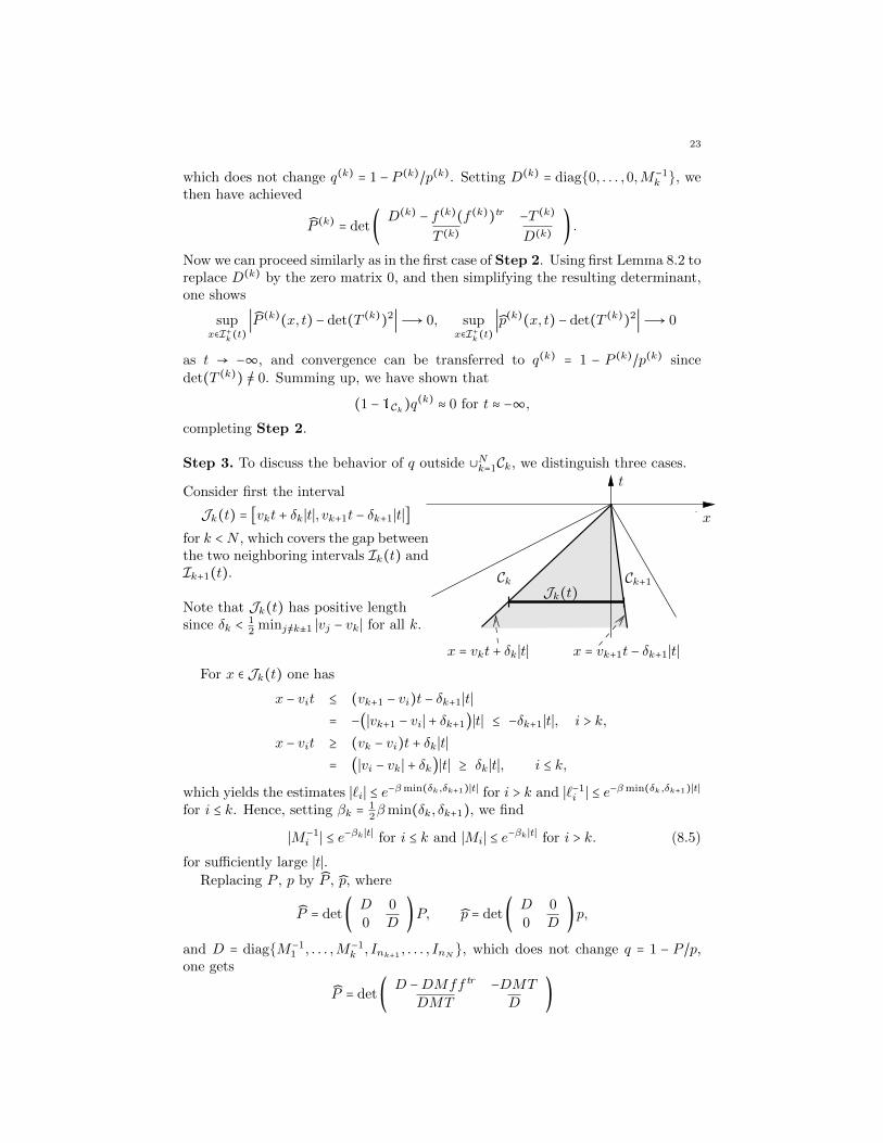
Step 3. To discuss the behavior of q outside ∪Nk=1Ck, we distinguish three cases.
Consider first the interval
Jk(t) = [vkt + δk ∣t∣, vk+1t − δk+1∣t∣]for k < N , which covers the gap betweenthe two neighboring intervals Ik(t) andIk+1(t).
Note that Jk(t) has positive lengthsince δk < 1
2minj/=k±1 ∣vj − vk ∣ for all k.
x
t
CkJk(t)
x = vk+1t − δk+1∣t∣
Ck+1
x = vkt + δk ∣t∣For x ∈ Jk(t) one has
x − vit ≤ (vk+1 − vi)t − δk+1∣t∣= −(∣vk+1 − vi∣ + δk+1)∣t∣ ≤ −δk+1∣t∣, i > k,
x − vit ≥ (vk − vi)t + δk ∣t∣= (∣vi − vk ∣ + δk)∣t∣ ≥ δk ∣t∣, i ≤ k,
which yields the estimates ∣`i∣ ≤ e−βmin(δk,δk+1)∣t∣ for i > k and ∣`−1i ∣ ≤ e−βmin(δk,δk+1)∣t∣
for i ≤ k. Hence, setting βk = 12βmin(δk, δk+1), we find
∣M−1i ∣ ≤ e−βk ∣t∣ for i ≤ k and ∣Mi∣ ≤ e−βk ∣t∣ for i > k. (8.5)
for sufficiently large ∣t∣.Replacing P , p by P , p, where
P = det( D 0
0 D)P, p = det( D 0
0 D)p,
and D = diagM−11 , . . . ,M−1
k , Ink+1 , . . . , InN , which does not change q = 1 − P /p,one gets
P = det( D −DMff tr −DMT
DMT D)

24 CORNELIA SCHIEBOLD
with DM = diagIn1 , . . . , Ink ,Mk+1, . . . ,MN. Similarly as is Step 2 one can nowuse (8.5) and Lemma 8.2 to replace D by J = diag0, . . . ,0, Ink+1 , . . . , InN and DMby I − J . After simplification of the resulting determinants, this results in
supx∈Jk(t)
∣P (x, t) − det(T )2∣Ð→ 0, supx∈Jk(t)
∣p(x, t) − det(T )2∣Ð→ 0
as t→ −∞, where T =( Tij )ki,j=1
.
Referring to [24, Theorem 4.1] for det(T ) /= 0, convergence can be transferred
from P , p to q = 1 − P /p.
Second we consider x ∈ Jmin(t) = ( −∞, v1t − δ1∣t∣ ]. In this case, x − vit ≤ −δ1∣t∣for all i, hence Lemma 8.2 can be applied directly to replace M by 0, which gives
supx∈Jmax(t)
∣P (x, t) − 1∣Ð→ 0, supx∈Jmax(t)
∣p(x, t) − 1∣Ð→ 0,
as t→ −∞, and we are done.
Finally we consider x ∈ Jmax(t) =[ vN t + δN ∣t∣,∞). Here x − vit ≥ δn∣t∣ for all i.
Replacing P , p by P , p with
P = det(M−1 0
0 M−1 )P, p = det(
M−1 0
0 M−1 )p,
which does not change q = 1 − P /p, one finds
P = det(M−1 − ff tr −T
T M−1 )
Using Lemma 8.2 to replace M−1 by 0, one arrives at
supx∈Jmin(t)
∣P (x, t) − det(T )2∣Ð→ 0, supx∈Jmin(t)
∣p(x, t) − det(T )2∣Ð→ 0,
as t→ −∞. Since det(T ) /= 0, see [24, Theorem 4.1], convergence can be transferred.Summing up,
(1 −N
∑k=1
1Ck)q ≈ 0 for t ≈ −∞,
which completes Step 3.
Conclusion.
q ≈N
∑k=1
1Ckq + (1 −N
∑k=1
1Ck)qSteps 1,3≈
N
∑k=1
1Ckq(k) + 0
Step 2≈N
∑k=1
1Ckq(k) +
N
∑k=1
(1 − 1Ck)q(k)
=N
∑k=1
q(k), t ≈ −∞.
This completes the proof of Proposition 8.1.

25
9. Collisions of the solitons within a wave packet
In this section turn to the fine analysis of the kth wave packet q(k) by studyingwhat happens if we deviate from the path x = vkt logarithmically.
Proposition 9.1. For ρ ∈ R, define γρ(t) = vkt + ρ log ∣t∣/Re(αk). Then, for the
determinants P (k), p(k) given in Proposition 8.1, it holds
p(k)(γρ(t), t) = C2(nk
∑κ=0
CκκFκ(t)Fκ(t) ∣t∣2ρκt−2κ2+2nkκ)[1 +O( log ∣t∣∣t∣ )],
P (k)(γρ(t), t) = C2(nk
∑κ=0
CκκFκ(t)Fκ(t) ∣t∣2ρκt−2κ2+2nkκ +
+nk−1
∑κ=0
(−1)κ+1C(κ+1)κFκ+1(t)Fκ(t) ∣t∣2ρκ+ρt−2κ2+2(nk−1)κ+(nk−1))[1 +O( log ∣t∣∣t∣ )]
with
C = det (Tij)k−1
ij=1,
Cκλ = [ 1
αk + αk]2κλ k−1
∏j=1
[αj − αkαj + αk
]2κnj
[αj − αkαj + αk
]2λnj
,
Fκ(t) = ∏κ−1κ′=1 κ
′!
∏κκ′=1(nk − κ′)!
(dnk−κk b(nk)k eiΥk(γρ(t),t))
κ
,
where dk = −2iRe(αk) and Υk(x, t) = Im ( αkx − iα2kt ).
Note that the parameter ρ controls the logarithmic deviation. It enters in theasymptotic via the terms ∣t∣2κρ, κ = 0, . . . , nk, and Υk(γρ(t), t).
The main part of the proof consists in expanding the determinants P (k), p(k).To this end we need some more notation. Consider the matrix
S = ( U VW Z
) ,
where U has the block structure
U =( Uij )kij=1
with Uij =( U (µν)ij ) µ=1,...,niν=1,...,nj
and V , W , Z are built analogously. For index tuples J = (σ1, . . . , σκ), J ′ =(σ′1, . . . , σ′κ), K = (τ1, . . . , τλ), K ′ = (τ ′1, . . . , τ ′λ) with σκ′ , σ
′κ′ , τλ′ , τ
′λ′ ∈ 1, . . . , nk
for 1 ≤ κ′ ≤ κ, 1 ≤ λ′ ≤ λ, we define the matrix S[J,K;J ′,K ′] by
S[J,K;J ′,K ′] = ( U[J, J ′] V [J,K ′]W [K,J ′] Z[K,K ′] ) .
Here U[J, J ′] denotes the matrix with the blocks U[J, J ′]ij , i, j = 1, . . . , k, where
(1) U[J, J ′]ij = Uij if i < k and j < k,(2) U[J, J ′]kj consists of the rows nr. σ1, . . . , σκ from Ukj for j < k,(3) U[J, J ′]ik consists of the columns nr. σ′1, . . . , σ
′κ from Uik for i < k,
(4) U[J, J ′]kk is obtained from Ukk by first selecting the rows nr. σ1, . . . , σκand then, from the resulting matrix, the columns nr. σ′1, . . . , σ
′κ (of course
we get the same result by first selecting columns).

26 CORNELIA SCHIEBOLD
J ′ K′
J
K
1
k − 1
k
1
k − 1
k
kk k − 1k − 11 1
Figure 6. To illustrate S[J,K;J ′,K ′], we indicate the positionof the blocks affected by the modifications.
Note that any ordering of the index tuples J, J ′ and even repetitions of indices areadmitted. V [J,K ′], W [K,J ′], Z[K,K ′] are defined accordingly.
By ∣J ∣ we denote the length of the index tuple J , in the case at hand ∣J ∣ = κ.Note that also the trivial case ∣J ∣ = 0 is admitted, where all rows of the respectiveblocks are eliminated.
Finally, with respect to the expansion in mind, we define I = diagJ(k), J(k) for
J(k) = diag0, . . . ,0, Ink. Routine arguments give:
Lemma 9.2. The following expansion rule holds:
det ( I + S ) =nk
∑κ=0
nk
∑λ=0
∑∣J ∣=κ
′ ∑∣K∣=λ
′det ( S[J,K;J,K] ),
where the inner sums are taken over all index tuples J , K from 1, . . . , nk and theprime means that only tuples with strictly increasing entries are admitted.
Recall that the cases κ = 0, λ = 0 correspond to the appearance of empty index sets.To determine the non-vanishing contributions in the expansion, we need the
following elementary lemma.
Lemma 9.3. Let B ∈ Mm,n(C), C ∈ Mn,m(C) be arbitrary, and b, c ∈ Cm. Ifeither m < n or n + 1 <m, then
det( cbtr BC 0
) = 0.
Proof. If m < n holds, the last n columns are linearly dependent. If n + 1 < m,the space U = d ∈ Cm ∣ Cd = 0 has dimension at least 2. The different ways ofcombining the zero vector from the columns of cbtr are parameterized by the spaceV = d ∈ Cm ∣ btrd = 0, which has codimension at most 1 in Cm. Hence U ∩V /= 0and the first m columns are linearly dependent.
27
The next lemmata (which have already been proved in [21]) are needed for theexplicit evaluation of certain determinants.
Lemma 9.4. For all γ ∈ C,
det (ν−1
∏ν′=1
(γ − µ − ν′ + 1) )m
µ,ν=1= (−1)
m(m+3)2
m−1
∏µ=1
µ!.
Proof. Multiplying the νth column by (γ −m − ν + 1) and subtracting it from the(ν + 1)th column for ν =m − 1, . . . ,1 (in the indicated order) gives
∆ = det (ν−1
∏ν′=1
(γ − µ − ν′ + 1) )m
µ,ν=1
= det (1, (m − µ)ν−2
∏ν′=1
(γ − µ − ν′ + 1) )µ≥1ν>1.
Next we expand the determinant with respect to the mth row, which is zero exceptfor the first entry. Extracting then the factor (m−µ), which is common to the µthrow for µ = 1, . . . ,m − 1, results in
∆ = (−1)m+1(m − 1)! det (ν−1
∏ν′=1
(γ − µ − ν′ + 1) )m−1
µ,ν=1,
and the assertion follows by induction.
Lemma 9.5. Let γ ∈ N with γ ≥ m. Then, for the m ×m matrix F = (fµν)m
µ,ν=1
given by
fµν =⎧⎪⎪⎪⎨⎪⎪⎪⎩
1
(γ − µ − ν + 1)! , µ + ν ≤ γ + 1,
0, µ + ν > γ + 1,
it holds
det(F ) = (−1)m(m+3)
2∏m−1µ=1 µ!
∏mµ=1(γ − µ)!
.
Proof. The identity
(γ − µ)! fµν =(γ − µ)!
(γ − µ − ν + 1)! =ν−1
∏ν′=1
(γ − µ − ν′ + 1)
holds for µ + ν ≤ γ + 1. It also holds for µ + ν > γ + 1 since in the product on theright the factor corresponding to ν′ = γ − µ + 1 < ν vanishes. Hence,
det(F ) = det ( 1
(γ − µ)!ν−1
∏ν′=1
(γ − µ − ν′ + 1))m
µ,ν=1,
and, after extracting the factors 1/(γ − µ)! common to the µth row, the assertionfollows from Lemma 9.4.
Proof of Proposition 9.1. First we provide estimates for the entries m(µ)k of Mk, see
Proposition 7.1 for their definition.
For `(α;x, t) = eαx−iα2t and µ ≥ 0, we define the polynomials qµ(α;x, t) byqµ = `−1∂µ`/∂αµ. Note that they satisfy the recursion relation qµ+1 = qµq1+∂qµ/∂α,where q0 = 1, q1 = x − 2iαt.
28 CORNELIA SCHIEBOLD
Observe that Re(αk)(x − vkt) = ρ log ∣t∣ for x = γρ(t). Hence, `(αk;γρ(t), t) =∣t∣ρeiΥk(γρ(t),t), and an inductive argument shows
qµ(αk;γρ(t), t) = (dkt)µ +O(∣t∣µ−1 log ∣t∣), ∂qµ
∂α(αk;γρ(t), t) = O(∣t∣µ).
As a result,
m(µ)k (γρ(t), t) =
dnk−µk b(nk)k eiΥk(γρ(t),t)
(nk − µ)!tnk−µ∣t∣ρ [1 +O( log ∣t∣
∣t∣ )]. (9.1)
In the proof, we focus on the treatment of P (k), which is the far more involved case.Write P (k) = det (I + S) with
S = ( −M (k)f (k)(f (k))tr −M (k)T (k)
M (k)(T (k))tr 0) ,
where we have used T (k) = (T (k))tr .Applying the expansion rule in Lemma 9.2, we obtain
P (k) =nk−1
∑κ=0
∑∣J ∣=κ+1
′ ∑∣K∣=κ
′det ( S[J,K;J,K] ) +
+nk
∑κ=0
∑∣J ∣=κ
′ ∑∣K∣=κ
′det ( S[J,K;J,K] ), (9.2)
where we have used Lemma 9.3 to see that the principal minors det (S[J,K;J,K])only contribute for ∣K ∣ = ∣J ∣ − 1 and ∣K ∣ = ∣J ∣. Our next aim is to evaluate thoseprincipal minors.
Recall that M (k)T (k) has the blocks Tij for i < k and MkTkj for i = k, where,from the upper left band structure of Mk, one finds
MkTkj = (nk−(µ−1)
∑κ=1
t(κν)kj m
(µ+κ−1)k )
µ=1,...,nkν=1,...,nj
.
Note also that Mke(1)nk (e
(1)nj )tr has a similar structure. Using linearity of the deter-
minant with respect to rows, we observe for J = (σ1, . . . , σκ), K = (τ1, . . . , τλ) withstrictly increasing indices, we have
det (S[J,K;J,K]) =nk−σ1+1
∑σ1=1
m(σ1+σ1−1)k . . .
nk−σκ+1
∑σκ=1
m(σκ+σκ−1)k
nk−τ1+1
∑τ1=1
m(τ1+τ1−1)k . . .
nk−τλ+1
∑τλ=1
m(τλ+τλ−1)k det (R[J , K;J,K]) (9.3)
with J = (σ1, . . . , σκ), K = (τ1, . . . , τλ), and
R = ( −f (k)(f (k))tr −T (k)(T (k))tr 0
) .
Since det (R[J , K;J,K]) = 0 if J or K contains two coinciding indices, J and Kcan be assumed to contain pairwise different indices.
29
We now look for those terms in (9.3) which are of leading order in t. From (9.1)we find that these correspond to the powers
κ
∑κ′=1
(ρ + nk + 1 − (σκ′ + σκ′)) +λ
∑λ′=1
(ρ + nk + 1 − (τλ′ + τλ′))
= (κ + λ)(ρ + nk + 1) −κ
∑κ′=1
(σκ′ + σκ′) −λ
∑λ′=1
(τλ′ + τλ′), (9.4)
with the constraint σκ′ + σκ′ , τλ′ + τλ′ ≤ nk + 1 for 1 ≤ κ′ ≤ κ, 1 ≤ λ′ ≤ λ, due to thelimitations of the summation in (9.3).
Let Perm(κ) denote the group of permutations of 1, . . . , κ and Perm′(κ) thesubset of those of the permutations π ∈ Perm(κ) which satisfy κ′ + π(κ′) ≤ nk + 1for all κ′ = 1, . . . , κ. Observe that ∑κκ′=1 σκ′ is minimal iff σκ′ = κ′ since the σκ′ arestrictly increasing, and since the σκ′ are pairwise different, ∑κκ′=1 σκ′ is minimal iffσκ′ = π(κ′) with π ∈ Perm′(κ).
Hence the expression in (9.4) attains its maximum precisely for J = J0, K =K0,
where J0 = (1, . . . , κ), K0 = (1, . . . , λ), and J = π(J0) = (π(1), . . . , π(κ)) with
π ∈ Perm′(κ), K = χ(K0) = (χ(1), . . . , χ(λ)) with χ ∈ Perm′(λ). To sum up,
det (S[J,K;J,K]) = Hκλ(t) [1 +O( 1
∣t∣ )] (9.5)
with
Hκλ(t) = ∑π∈Perm′(κ)
∑χ∈Perm′(λ)
κ
∏κ′=1
m(κ′+π(κ′)−1)k
λ
∏λ′=1
m(λ′+χ(λ′)−1)k
det (R[π(J0), χ(K0);J0,K0]).(9.6)
Using (9.1) and ∑κκ′=1(nk − (κ′ + π(κ′) − 1)) = (nk + 1)κ − 2∑κκ′=1 κ′ = (nk − κ)κ, we
find that
κ
∏κ′=1
m(κ′+π(κ′)−1)k = Gκ(t) t(nk−κ)κ∣t∣κρ
κ
∏κ′=1
(nk + 1 − (κ′ + π(κ′)))![1 +O( log ∣t∣
∣t∣ )]
with
Gκ(t) = (dnk−κk b(nk)k eiΥk(γρ(t),t))
κ
(note that Gκ(t) does not contribute to the growth in t since ∣Gκ(t)∣ is constant).Inserting this into (9.6), we get
Hκλ(t) =Dκλ Gκ(t)Gλ(t) ∣t∣(κ+λ)ρ tκ(nk−κ)+λ(nk−λ) [1+O( log ∣t∣∣t∣ )], (9.7)
where
Dκλ = ∑π∈Perm′(κ)χ∈Perm′(λ)
κ
∏κ′=1
1
(nk + 1 − (κ′ + π(κ′)))!
λ
∏λ′=1
1
(nk + 1 − (λ′ + χ(λ′)))!
det (R[π(J0), χ(K0);J0,K0]).

30 CORNELIA SCHIEBOLD
We can drop the restriction on the permutations if we pass to the quantities
fµν =⎧⎪⎪⎪⎨⎪⎪⎪⎩
1
(nk + 1 − (µ + ν))! , µ + ν ≤ nk + 1,
0, µ + ν > nk + 1..
Moreover, det(R[π(J0), χ(K0);J0,K0]) = sgn(π)sgn(χ)det(R[J0,K0;J0,K0]) byreordering rows. Hence,
Dκλ = ∑π∈Perm(κ)
sgn(π)κ
∏κ′=1
fκ′π(κ′) ∑χ∈Perm(λ)
sgn(χ)λ
∏λ′=1
fλ′χ(λ′)
det (R[J0,K0;J0,K0])
= det ( fµν )κµ,ν=1
det ( fµν )λµ,ν=1
det (R[J0,K0;J0,K0]).
For the evaluation of the first two determinants see Lemma 9.5. The evaluation ofthe last one is in fact quite involved, and we refer to [24, Theorem 5.1] for the fact2
that det(R[J0,K0;J0,K0]) = (−1)κ+λC2Cκλ for λ = κ − 1, κ. Hence,
Dκλ = (−1)κ(κ+1)
2 (−1)λ(λ+1)
2∏κ−1κ′=1 κ
′!
∏κκ′=1(nk − κ′)!
∏λ−1λ′=1 λ
′!
∏λλ′=1(nk − λ′)!
C2Cκλ. (9.8)
Using (9.7), (9.8) in (9.5), we infer
det (S[J,K;J,K]) = (−1)κ(κ+1)
2 (−1)λ(λ+1)
2 C2CκλFκ(t)Fλ(t)
∣t∣(κ+λ)ρ tκ(nk−κ)+λ(nk−λ) [1+O( log ∣t∣∣t∣ )], (9.9)
and the proof is completed by inserting (9.9) into (9.2).
Now we are in position to give the asymptotic behavior of the kth wave packet.
2 For the reader’s convenience we sketch how to apply [24, Theorem 5.1] in the situation at
hand. First we state
Corollary 9.6. Let li,mj ∈ N, i = 1, . . . , L, j = 1, . . . ,M , and l = ∑Li=1 li, m = ∑M
j=1mj .
For βi, γj ∈ C, i = 1, . . . , L, j = 1, . . . ,M , with βi + γj /= 0 for all i, j, we define the matrixU = (Uij) i=1,...,L
j=1,...M∈Ml,m(C) with the blocks
Uij =⎛⎝(
1
βi + γj)i′+j′−1
(i′ + j′ − 2
i′ − 1)⎞⎠ i′=1,...,lij′=1,...,mj
∈Mli,mj (C).
Furthermore, let g be the vector consisting of the first standard basis vectors e(1)mj ∈ Cmj for
j = 1, . . . ,M . Then, for m ∈ l, l + 1,
det(−ggtr −U
U tr 0) = (−1)l+m
L
∏i,j=1i<j
(βi − βj)2liljM
∏i,j=1i<j
(γi − γj)2mimj/L
∏i=1
M
∏j=1(βi + γj)2limj .
Corollary 9.6 immediately follows from [24, Theorem 5.1] using the fact that U and U tr havethe same structure, and the following identity
(−ggtr −U
U tr 0) = − (0n×m In
Im 0m×n)(0 −U tr
U ggtr)(0n×m In
Im 0m×n) ,
which holds for all g ∈ Cm and U ∈Mm,n(C).To conclude, we apply Corollary 9.6 with L =M = k, βj = αj , γj = αj , lj =mj = nj for all j < k
and lk = κ, mk = λ.
31
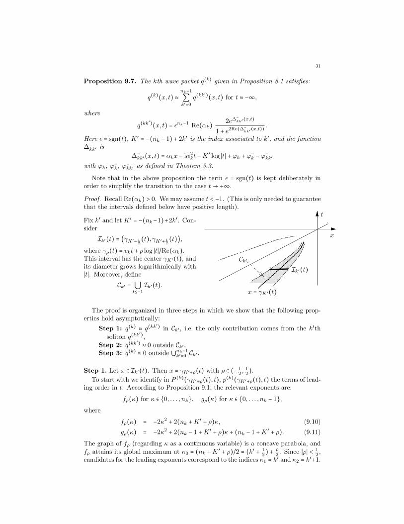
Proposition 9.7. The kth wave packet q(k) given in Proposition 8.1 satisfies:
q(k)(x, t) ≈nk−1
∑k′=0
q(kk′)(x, t) for t ≈ −∞,
where
q(kk′)(x, t) = εnk−1 Re(αk)
2e∆−kk′(x,t)
1 + e2Re(∆−kk′(x,t))
.
Here ε = sgn(t), K ′ = −(nk − 1)+ 2k′ is the index associated to k′, and the function∆−kk′ is
∆−kk′(x, t) = αkx − iα2
kt −K ′ log ∣t∣ + ϕk + ϕ−k − ϕ−kk′with ϕk, ϕ−k, ϕ−kk′ as defined in Theorem 3.3.
Note that in the above proposition the term ε = sgn(t) is kept deliberately inorder to simplify the transition to the case t→ +∞.
Proof. Recall Re(αk) > 0. We may assume t < −1. (This is only needed to guaranteethat the intervals defined below have positive length).
Fix k′ and let K ′ = −(nk−1)+2k′. Con-sider
Ik′(t) = (γK′− 12(t), γK′+ 1
2(t)),
where γρ(t) = vkt + ρ log ∣t∣/Re(αk).This interval has the center γK′(t), andits diameter grows logarithmically with∣t∣. Moreover, define
Ck′ = ⋃t≤−1
Ik′(t).
x
t
Ck′Ik′(t)
x = γK′(t)
The proof is organized in three steps in which we show that the following prop-erties hold asymptotically:
Step 1: q(k) ≈ q(kk′) in Ck′ , i.e. the only contribution comes from the k′th
soliton q(kk′),
Step 2: q(kk′) ≈ 0 outside Ck′ ,
Step 3: q(k) ≈ 0 outside ⋃nk−1k′=0 Ck′ .
Step 1. Let x ∈ Ik′(t). Then x = γK′+ρ(t) with ρ ∈ (− 12, 1
2).
To start with we identify in P (k)(γK′+ρ(t), t), p(k)(γK′+ρ(t), t) the terms of lead-ing order in t. According to Proposition 9.1, the relevant exponents are:
fρ(κ) for κ ∈ 0, . . . , nk, gρ(κ) for κ ∈ 0, . . . , nk − 1,where
fρ(κ) = −2κ2 + 2(nk +K ′ + ρ)κ, (9.10)
gρ(κ) = −2κ2 + 2(nk − 1 +K ′ + ρ)κ + (nk − 1 +K ′ + ρ). (9.11)
The graph of fρ (regarding κ as a continuous variable) is a concave parabola, andfρ attains its global maximum at κ0 = (nk +K ′ + ρ)/2 = (k′ + 1
2) + ρ
2. Since ∣ρ∣ < 1
2,
candidates for the leading exponents correspond to the indices κ1 = k′ and κ2 = k′+1.
32 CORNELIA SCHIEBOLD
Furthermore, we use fρ(k′ + 1) = fρ(k′)+ 2ρ, fρ(k′ + 2) = fρ(k′ − 1)+ 6ρ to estimatethe minimal distance to the other exponents from below by
min (fρ(k′), fρ(k′ + 1)) −max (fρ(k′ − 1), fρ(k′ + 2)) =
= fρ(k′ + 1) − fρ(k′ − 1) for ρ ≤ 0fρ(k′) − fρ(k′ + 2) for ρ ≥ 0
= 4(1 − ∣ρ∣) > 2.
Analogously, gρ has its maximum at κ0 = (nk − 1 +K ′ + ρ)/2 = k′ + ρ2, showing that
the leading exponent corresponds to κ1 = k′, and for the minimal distance to theother exponents we get the estimate gρ(k′) −max (gρ(k′ − 1), gρ(k′ + 1)) > 1.
Keeping only the terms of leading order in t (which correspond to κ = k′, k′ + 1
for p(k) and κ = k′ for p(k)−P (k) in Proposition 9.1), we get for q(k) = 1−P (k)/p(k) =(p(k) − P (k))/p(k),
q(k)(γK′+ρ(t), t) =
=−(−1)k′+1C(k′+1)k′Gk′(t) ∣t∣K′+ρ tnk−2k′−1[1 +O( log ∣t∣
∣t∣ )]
(Ck′k′ +C(k′+1)(k′+1)Gk′(t)Gk′(t) ∣t∣2(K′+ρ) t2(nk−2k′−1))[1 +O( log ∣t∣∣t∣ )]
= εK′(−1)k
′ C(k′+1)k′Gk′(t) ∣t∣ρ
Ck′k′ +C(k′+1)(k′+1)Gk′(t)Gk′(t) ∣t∣2ρ[1 +O( log ∣t∣
∣t∣ )] (9.12)
with
Gk′(t) =Fk′+1(t)Fk′(t)
= k′!
(nk − k′ − 1)!dnk−2k′−1k b
(nk)k eiΥ(k)(γK′+ρ(t),t). (9.13)
Recall b(nk)k = a(1)k c
(nk)k , see Proposition 7.1, dk = −2iRe(αk), see Proposition 9.1,
and K ′ = −(nk −1)+2k′. Using also the definitions of ϕk, ϕ−kk′ , and ϕ−k in Theorem3.3, we find
Gk′(t)e−iΥ(k)(γK′+ρ(t),t) = k′!
(k′ −K ′)!(−i)−K′(2Re(αk))
−K′a(1)k c
(nk)k
= (−1)k′(2Re(αk))
2k′+1 k′!
(k′ −K ′)!(2Re(αk))
−2K′(−i)nk−1 a
(1)k c
(nk)k
(2Re(αk))nk
= (2Re(αk))2k′+1
eϕk−ϕ−kk′ ,
C(k′+1)k′
Ck′k′= eϕ
−k
(2Re(αk))2k′ ,
C(k′+1)(k′+1)
Ck′k′= eϕ
−k+ϕ−k
(2Re(αk))4k′+2
.
Inserting this into (9.12), we get q(k)(γK′+ρ(t), t) = Q(kk′)(t)[1 +O( log ∣t∣
∣t∣ )], where
Q(kk′)(t) = (−1)k
′εK
′2Re(αk)
P(kk′)(t) ∣t∣ρ
1 +P(kk′)(t)P(kk′)(t) ∣t∣2ρ, (9.14)
P(kk′)(t) = exp ( iΥ(k)(γK′+ρ(t), t) + ϕk + ϕ−k − ϕ−kk′ ) . (9.15)
Since Q(kk′)(t) is bounded, it even holds q(k)(γK′+ρ(t), t) = Q(kk′)(t) +O( log ∣t∣
∣t∣ ).
33
On the other hand it is straightforward to check that q(kk′)(γK′+ρ(t), t) = Q(kk
′)(t).Hence we may conclude
supx∈Ik′(t)
∣q(k)(x, t) − q(kk′)(x, t)∣→ 0 as t→ −∞.
In summary,
1Ck′ q(k) ≈ 1Ck′ q
(kk′) for t ≈ −∞,where 1Ck′ is the characteristic function of Ck′ , and Step 1 is complete.
Step 2. To discuss the behavior of q(kk′) outside of Ik′(t), we distinguish two cases:
First, let x ∈ I−k′(t) =( −∞, γK′− 12(t) ]. Then x = γK′+ρ(t) with ρ ≤ − 1
2, and
∣q(kk′)(γK′+ρ(t), t)∣ = ∣Q(kk
′)(t)∣ (9.14)= 2Re(αk)c∣t∣ρ
1 + c2∣t∣2ρ = O(∣t∣ρ),
where we have used (9.15) to see that c = ∣P(kk′)(t)∣ > 0 does not depend on t.
Hence ∣q(kk′)(γK′+ρ(t), t)∣ = O(∣t∣− 12 ) for all ρ ≤ − 1
2.
Second, let x ∈ I+k′(t) =[ γK′+ 12(t),∞ ). Then x = γK′+ρ(t) with ρ ≥ 1
2, and after
rewritingc∣t∣ρ
1 + c2∣t∣2ρ = ∣t∣−ρ/c1 + ∣t∣−2ρ/c2 ,
a similar argument as above shows ∣q(kk′)(γK′+ρ(t), t)∣ = O(∣t∣− 12 ) for all ρ ≥ 1
2.
This completes Step 2 as we have shown
(1 − 1Ck′ )q(kk′) ≈ 0 for t ≈ −∞.
Step 3. To discuss the behavior of q(k) outside ∪nk−1k′=0 Ck′ , we distinguish three cases.
Consider first the interval
Jk′(t) = [γK′+ 12(t), γ(K′+2)− 1
2(t)]
for k′ < nk − 1. Note that, if K ′ is the index associated to k′, then K ′ + 2 is theindex associated to k′ + 1. Thus, Jk′(t) is the interval covering the gap betweenIk′(t) and Ik′+1(t). Let x ∈ Jk′(t), then x = γK′+ρ(t) with ρ ∈ [ 1
2, 3
2].
To find the terms of leading order in t for P (k)(γK′+ρ(t), t), p(k)(γK′+ρ(t), t),recall that the function fρ given in (9.10) has its maximum at κ0 = (k′ + 1
2) + ρ
2.
Since 12≤ ρ ≤ 3
2, the leading exponent corresponds to κ1 = k′ + 1, and its minimal
distance to the other exponents can be estimated from below by
fρ(k′ + 1) −max (fρ(k′), fρ(k′ + 2)) = min (2ρ,4 − 2ρ) ≥ 1.
Since the function gρ given in (9.11) has its maximum at κ0 = k′ + ρ2, candidates for
the leading exponent are κ1 = k′ and κ2 = k′ + 1, and for the minimal distance tothe other exponents we get
mingρ(k′), gρ(k′ + 1) −maxgρ(k′ − 1), gρ(k′ + 2) =
= gρ(k′ + 1) − gρ(k′ − 1) = 4ρ ≥ 2 for ρ ≤ 1,gρ(k′) − gρ(k′ + 2) = 4(2 − ρ) ≥ 2 for ρ ≥ 1.
Keeping only the terms of leading order in t, we get
q(k)(γK′+ρ(t), t) =
34 CORNELIA SCHIEBOLD
=−((−1)k′+1C(k′+1)k′ + (−1)k′+2C(k′+2)(k′+1)Gk′+1(t)Gk′(t) ∣t∣2(K′+ρ) t2(nk−2k′−2))
C(k′+1)(k′+1)Gk′(t) ∣t∣K′+ρ tnk−2k′−1
⋅[1 +O( log ∣t∣∣t∣ )]
= (−1)k′ε−K
′ C(k′+1)k′ −C(k′+2)(k′+1)Gk′+1(t)Gk′(t) ∣t∣2ρ−2
C(k′+1)(k′+1)Gk′(t) ∣t∣ρ[1 +O( log ∣t∣
∣t∣ )]
with Gk′(t) as in (9.13). Observe that ∣Gk′(t)∣ = ck′ does not depend on t. Hence,for all 1
2≤ ρ ≤ 3
2,
∣q(k)(γK′+ρ(t), t)∣
≤ ( 1
ck′
C(k′+1)k′
C(k′+1)(k′+1)∣t∣−ρ + ck′+1
C(k′+2)(k′+1)
C(k′+1)(k′+1)∣t∣ρ−2)[1 +O( log ∣t∣
∣t∣ )]
= O(∣t∣− 12 ).
Second, consider the interval Jmin(t) = (−∞, γ(−(nk−1)− 12 )
(t)]. Note that Jmin(t)covers the gap between −∞ and I0(t). Let x ∈ Jmin(t), then x = γ(−(nk−1)+ρ)(t)with ρ ∈ ( −∞,− 1
2].
In this case the leading exponent both for fρ and gρ corresponds to κ1 = 0, andfor the minimal distance to the other exponents we get fρ(0)− fρ(1) = −2ρ ≥ 1 andgρ(0) − gρ(1) = −2(ρ − 1) ≥ 3. Hence,
q(k)(γ(−(nk−1)+ρ)(t), t) = εnk−1C10
C00G0(t) ∣t∣ρ[1 +O( log ∣t∣
∣t∣ )],
showing ∣q(k)(γ(−(nk−1)+ρ)(t), t)∣ = O(t− 12 ) for all ρ ≤ − 1
2.
Finally consider Jmax(t) = [γ((nk−1)+ 12 )
(t),∞), the interval covering the gap
between Ink−1(t) and +∞. Let x ∈ Jmax(t), then x = γ((nk−1)+ρ)(t) with ρ ∈ [ 12,∞).
Here the leading exponents correspond to κ1 = nk for fρ and κ2 = nk−1 for gρ, andfor the minimal distance to the other exponents we have fρ(nk)−fρ(nk−1) = 2ρ ≥ 1and gρ(nk − 1) − gρ(nk − 2) = 2(ρ + 1) ≥ 3. Hence
q(k)(γ((nk−1)+ρ)(t), t) = (−ε)nk−1Cnk(nk−1)
Cnknk
1
Gnk−1(t)∣t∣−ρ[1 +O( log ∣t∣
∣t∣ )],
showing ∣q(k)(γ((nk−1)+ρ)(t), t)∣ = O(∣t∣− 12 ) for all ρ ≥ 1
2.
As a result,
(1 −nk−1
∑k′=0
1Ck′ )q(k) ≈ 0 for t ≈ −∞.
This completes Step 3 and, by a similar conclusion as in the proof of Proposition8.1, also the proof of Proposition 9.7.
Proof of Theorem 3.3. Theorem 3.3 follows from Propositions 8.1 and 9.7 uponreordering as follows: Set k′′ = (nk − 1) − k′. For the index K ′′ = −(nk − 1) + 2k′′
associated to k′′, we then have
K ′′ = −K ′ and k′′ −K ′′ = k′.In particular, ϕ−kk′′ = −ϕ−kk′ . Geometrically, this replacement reverses the order ofthe solitons within the kth wave packet.
35
Remark 9.8. To see that the asymptotic description in Theorem 3.3 includes whatis proved in [30] (for N -solitons) and [15] (for a single wave packet), one proceedsas follows:
(1) In Section 6, it is shown that the solutions obtained via ISM starting fromthe data (6.1) are realized in Theorem 2.3 for
A = −2iJ, a = −2i ( e(1)nj )Nj=1, c =(( rjj′ )
nj
j′=1)N
j=1,
where J is in Jordan form with N Jordan blocks of sizes nj×nj correspond-ing to eigenvalues kj .
(2) To apply Theorem 3.3, A needs to be brought in Jordan form. This canbe done using the transformation matrix U = diagUj ∣j = 1, . . . ,N with
Uj = diag(−2i)j′−1∣j′ = 1, . . . , nj. Then A = U−1AU is in Jordan form.Now Lemma 5.2 tells that the solution is not changed if we simultane-
ously replace A, a, c by A, a = (U−1)tr a, c = Uc, which gives us as relevantdata
αj = −2ikj , a(1)j = −2i, c
(nj)j = (−2i)nj−1rjnj .
(3) Since αj = −2ikj , we have Re(αj) < 0. As a consequence, in Theorem 3.3the index sets Λ+
j and Λ−j have to be interchanged (see also the paragraph
on Assumption a) in Theorem 3.3 in Section 5).(4) For the asymptotic form in t ≈ −∞, the reordering j′′ = (nj − 1) − j′ can be
used to switch from Γ−jj′(x, t) in Theorem 3.3 to
Γ−jj′′(x, t) = αjx − iα2j t − J ′′ log ∣t∣ + ϕj + ϕ−j + ϕ−jj′′
(compare the proof of Theorem 3.3).(5) Note finally that the transformation t↦ −t (in particular sgn(t)↦ sgn(−t))
is needed to bring the NLS in [15], [30] to the form used in this work.
10. Solutions of higher degeneracy
This section aims at a first understanding of solutions involving solitons, or moregenerally wave packets of the same velocity. Motivated by [5], we start with theheuristic question whether groups of such wave packets should be considered asstable bound states. Then we indicate how our method contributes to the under-standing of solutions of higher degeneracy by performing the asymptotic analysisfor the first relevant case. We conclude with some plots for higher degeneracyphenomena in Figures 8 - 10.
A family of degenerate solutions. Since wave packets which travel with thesame velocity cannot be separated by asymptotic analysis, it is natural to askwhether they constitute stable bound states, so-called formations (see [3, p.34]). Afamous example of such formations are the breather solutions of the sine-Gordonequation. In [19] it has been shown that these formations can be included in theasymptotic analysis.
For the NLS, a solution obtained by superposing two stationary solitons is dis-cussed in [5, Example 7.2], see also Example 5.1. However, the subsequent exampleshows that this solution is not stable under collision with a non-stationary soliton.

36 CORNELIA SCHIEBOLD
Figure 7. The solution discussed in Example 5.1 collides withnon-stationary solitons, see Example 10.1 for details. In both cases,the two stationary solitons of which the solution in Example 5.1consists are separated by the collision, thereby revealing its natureas a true 2-soliton. Note how sensitively the position-shift of thetwo stationary solitons depends on the non-stationary soliton: Inthe first picture the larger stationary soliton ends up on the left,in the second on the right side.
Example 10.1. Let Im(β) /= 0. Starting from the data
A =⎛⎜⎝
4 0 00 2 00 0 β
⎞⎟⎠,
we obtain a solution which superposes two stationary solitons of heights 4 and 2respectively and a non-stationary soliton of height ∣Re(β)∣. Recall that the velocityof the non-stationary soliton is −2Im(β). The corresponding solution is illustratedin Figure 10.1 for the parameters a1 = a2 = 1, c1 = 18, c2 = −32, and
β = 2 + i with a3 = 1, c3 = 4 (for the plot to the left), β = 4 + 0.4i with a3 = 1, c3 = 60 (for the plot to the right).
In both cases the plotted region is −5 ≤ x ≤ 5, −3 ≤ t ≤ 3.For large negative times this solution asymptotically looks like the superposition
of the solution discussed in [5, Example 7.2], see also Example 5.1, and a movingsoliton. But for large positive times, the two stationary solitons constituting thesolution in [5, Example 7.2] appear clearly separated due to the fact that they havesuffered different position-shifts in their collision with the moving soliton.
Asymptotic analysis of the degenerate 3-soliton. To confirm the heuristicsof Example 10.1, we analyze in some detail the asymptotics of a 3-soliton with twosolitons of the same velocity.
To this end, we consider the solution q generated by A = diagα1, α2, α3 withIm(α1) = Im(α2) /= Im(α3) and a = (1,1,1), c = (eϕ1 , eϕ2 , eϕ3) in Theorem 2.3.
37
To avoid cancelation phenomena, let α1 /= α2. As before we will also assumeRe(αj) > 0 for all j (compare the paragraph on Assumption a) in Theorem 3.3 inSection 5). We furthermore assume Im(α3) > Im(α1), the case Im(α3) < Im(α1)being analogous.
Observe that q = 1 − P /p, where P , p are given by (2.5) with
L = ( 1
αi + αj`i)
i,j=1,2,3, L0 = ( `i )
i,j=1,2,3,
and `i(x, t) = exp(αix − iα2i + ϕi).
Behavior for t→ −∞.
Step 1: Moving with the two solitons of equal velocity. Consider curvesx+ 2Im(α1)t = c. On such a curve, ∣`3(x, t)∣→ 0 for t→ −∞. The arguments for P ,p being parallel, we look at P and find
P → det
⎛⎜⎜⎜⎜⎜⎜⎜⎜⎜⎝
−`1 1 − `1 −`1 − 1α1+α1
`1 − 1α1+α2
`1 − 1α1+α3
`1−`2 −`2 1 − `2 − 1
α2+α1`2 − 1
α2+α2`2 − 1
α2+α3`2
0 0 1 0 0 01
α1+α1`1
1α1+α2
`11
α1+α3`1 1 0 0
1α2+α1
`21
α2+α2`2
1α2+α3
`2 0 1 0
0 0 0 0 0 1
⎞⎟⎟⎟⎟⎟⎟⎟⎟⎟⎠
= det
⎛⎜⎜⎜⎜⎝
1 − `1 −`1 − 1α1+α1
`1 − 1α1+α2
`1−`2 1 − `2 − 1
α2+α1`2 − 1
α2+α2`2
1α1+α1
`11
α1+α2`1 1 0
1α2+α1
`21
α2+α2`2 0 1
⎞⎟⎟⎟⎟⎠.
The corresponding solution is the superposition of the first two solitons as obtainedfrom the 2 × 2-matrix A = diagα1, α2 and a = (1,1), c = (eϕ1 , eϕ2) in Theorem2.3. Note that, for α1 = 4, α2 = 2, and c = (18,−32), this is is precisely the solutiondiscussed in Example 5.1.
Step 2: Moving with the remaining soliton. On curves x + 2Im(α3)t = c,we observe ∣1/`1(x, t)∣, ∣1/`2(x, t)∣ → 0 for t → −∞. In this case we divide in both
determinants P , p the first row by `1, the second row by `2, the fourth row by `1,and the fifth row by `2. Note that this does not effect the quotient P /p. Again wefocus on the more complicated determinant P , for which we get P → P0, where
P0 = det
⎛⎜⎜⎜⎜⎜⎜⎜⎜⎜⎝
−1 −1 −1 − 1α1+α1
− 1α1+α2
− 1α1+α3
−1 −1 −1 − 1α2+α1
− 1α2+α2
− 1α2+α3
−`3 −`3 1 − `3 − 1α3+α1
`3 − 1α3+α2
`3 − 1α3+α3
`31
α1+α1
1α1+α2
1α1+α3
0 0 01
α2+α1
1α2+α2
1α2+α3
0 0 01
α3+α1`3
1α3+α2
`31
α3+α3`3 0 0 1
⎞⎟⎟⎟⎟⎟⎟⎟⎟⎟⎠
.
To identify the corresponding solution, we calculate P0. Using the abbreviationγij = (αi − αj)/(αi + αj), we perform the following operations simultaneously forboth determinants:
(1) multiply the first row by (α1+α1)/(α2+α1) and subtract it from the secondrow, extract the factor γ21 from the second row,

38 CORNELIA SCHIEBOLD
(2) multiply the first row by `3(α1 + α1)/(α3 + α1) and subtract it from thethird row, set f3 = γ31`3,
(3) multiply the second row by f3(α2 +α2)/(α3 +α2) and subtract it from thethird row, set g3 = γ32f3,
(4) multiply the first column by (α1 + α1)/(α1 + α2) and subtract it from thesecond column, extract the factor γ21 from the second column,
(5) multiply the first column by (α1 + α1)/(α1 + α3) and subtract it from thethird column,
(6) multiply the second column by γ31(α2 +α2)/(α2 +α3) and subtract it fromthe third column.
After expansion, this results in
P0 = γ det(I + T )with
γ = γ221γ
221
(α1 + α1)2(α2 + α2)2, T = ( −γ31γ32 g3 −γ31γ32
α3+α3g3
γ31γ32α3+α3
g3 0) .
Factorizing T = T1T2, where
T1 = ( −g3 − 1α3+α3
g31
α3+α3g3 0
) , T2 = ( γ31γ32 00 γ31γ32
) ,
and using the identity det(I + T1T2) = det(I + T2T1), we get
P0 = γ det(1 − h3 − 1
α3+α3h3
1α3+α3
h3 1)
for h3 = (γ31γ32)2`3.The factor γ appears also in front of the other determinant and hence cancels
out in the quotient. As a result, we find the third soliton as obtained from A = α3,a = 1, c = eψ3 in Theorem 2.3, with the initial shift
ψ3 = ϕ3 + log((α3 − α1)(α3 − α2)(α3 + α1)(α3 + α2)
)2
.
Step 3: Other velocities. On curves x + βt = c with β ∈ R/Im(α1), Im(α3),one checks q = 1 − P /p → 0 for t → −∞, showing that there is no asymptoticcontribution.
Behavior for t→∞.
Step 1: Moving with the two solitons of equal velocity. On curvesx + 2Im(α1)t = c, we have 1/∣`3(x, t)∣ → 0 for t → ∞. Here we divide in both
determinants P , p the third row by `3 and the sixth row by `3. Focussing on P , weget P → P0, where
P0 = det
⎛⎜⎜⎜⎜⎜⎜⎜⎜⎜⎝
1 − `1 −`1 −`1 − 1α1+α1
`1 − 1α1+α2
`1 − 1α1+α3
`1−`2 1 − `2 −`2 − 1
α2+α1`2 − 1
α2+α2`2 − 1
α2+α3`2
−1 −1 −1 − 1α3+α1
− 1α3+α2
− 1α3+α3
1α1+α1
`11
α1+α2`1
1α1+α3
`1 1 0 01
α2+α1`2
1α2+α2
`21
α2+α3`2 0 1 0
1α3+α1
1α3+α2
1α3+α3
0 0 0
⎞⎟⎟⎟⎟⎟⎟⎟⎟⎟⎠
.
To identify the solution, we
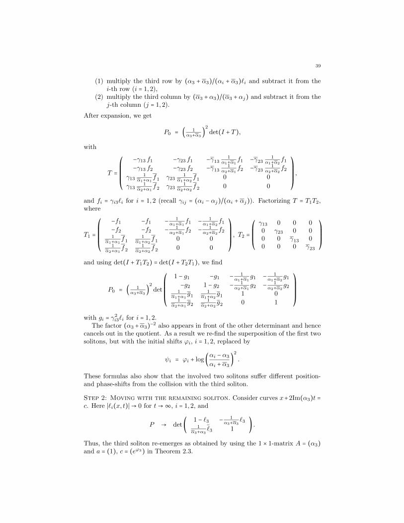
39
(1) multiply the third row by (α3 + α3)/(αi + α3)`i and subtract it from thei-th row (i = 1,2),
(2) multiply the third column by (α3 +α3)/(α3 +αj) and subtract it from thej-th column (j = 1,2).
After expansion, we get
P0 = ( 1α3+α3
)2
det(I + T ),
with
T =⎛⎜⎜⎜⎜⎝
−γ13 f1 −γ23 f1 −γ131
α1+α1f1 −γ23
1α1+α2
f1
−γ13 f2 −γ23 f2 −γ131
α2+α1f2 −γ23
1α2+α2
f2
γ131
α1+α1f1 γ23
1α1+α2
f1 0 0
γ131
α2+α1f2 γ23
1α2+α2
f2 0 0
⎞⎟⎟⎟⎟⎠,
and fi = γi3`i for i = 1,2 (recall γij = (αi − αj)/(αi + αj)). Factorizing T = T1T2,where
T1 =⎛⎜⎜⎜⎜⎝
−f1 −f1 − 1α1+α1
f1 − 1α1+α2
f1
−f2 −f2 − 1α2+α1
f2 − 1α2+α2
f21
α1+α1f1
1α1+α2
f1 0 01
α2+α1f2
1α2+α2
f2 0 0
⎞⎟⎟⎟⎟⎠, T2 =
⎛⎜⎜⎜⎝
γ13 0 0 00 γ23 0 00 0 γ13 00 0 0 γ23
⎞⎟⎟⎟⎠
and using det(I + T1T2) = det(I + T2T1), we find
P0 = ( 1α3+α3
)2
det
⎛⎜⎜⎜⎜⎝
1 − g1 −g1 − 1α1+α1
g1 − 1α1+α2
g1
−g2 1 − g2 − 1α2+α1
g2 − 1α2+α2
g21
α1+α1g1
1α1+α2
g1 1 01
α2+α1g2
1α2+α2
g2 0 1
⎞⎟⎟⎟⎟⎠
with gi = γ2i3`i for i = 1,2.
The factor (α3 +α3)−2 also appears in front of the other determinant and hencecancels out in the quotient. As a result we re-find the superposition of the first twosolitons, but with the initial shifts ϕi, i = 1,2, replaced by
ψi = ϕi + log (αi − α3
αi + α3)
2
.
These formulas also show that the involved two solitons suffer different position-and phase-shifts from the collision with the third soliton.
Step 2: Moving with the remaining soliton. Consider curves x+2Im(α3)t =c. Here ∣`i(x, t)∣→ 0 for t→∞, i = 1,2, and
P → det(1 − `3 − 1
α3+α3`3
1α3+α3
`3 1) .
Thus, the third soliton re-emerges as obtained by using the 1 × 1-matrix A = (α3)and a = (1), c = (eϕ3) in Theorem 2.3.
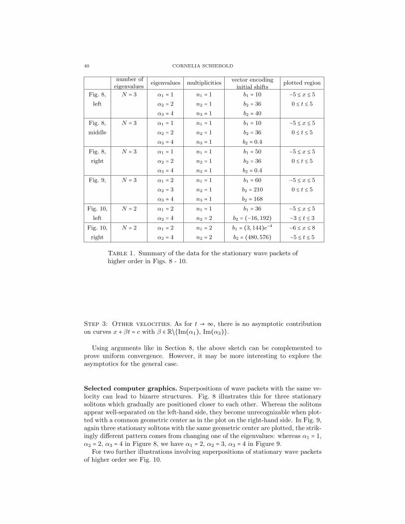
40 CORNELIA SCHIEBOLD
number ofeigenvalues
eigenvalues multiplicitiesvector encodinginitial shifts
plotted region
Fig. 8, N = 3 α1 = 1 n1 = 1 b1 = 10 −5 ≤ x ≤ 5
left α2 = 2 n2 = 1 b2 = 36 0 ≤ t ≤ 5
α3 = 4 n3 = 1 b2 = 40
Fig. 8, N = 3 α1 = 1 n1 = 1 b1 = 10 −5 ≤ x ≤ 5
middle α2 = 2 n2 = 1 b2 = 36 0 ≤ t ≤ 5
α3 = 4 n3 = 1 b2 = 0.4
Fig. 8, N = 3 α1 = 1 n1 = 1 b1 = 50 −5 ≤ x ≤ 5
right α2 = 2 n2 = 1 b2 = 36 0 ≤ t ≤ 5
α3 = 4 n3 = 1 b2 = 0.4
Fig. 9, N = 3 α1 = 2 n1 = 1 b1 = 60 −5 ≤ x ≤ 5
α2 = 3 n2 = 1 b2 = 210 0 ≤ t ≤ 5
α3 = 4 n3 = 1 b2 = 168
Fig. 10, N = 2 α1 = 2 n1 = 1 b1 = 36 −5 ≤ x ≤ 5
left α2 = 4 n2 = 2 b2 = (−16,192) −3 ≤ t ≤ 3
Fig. 10, N = 2 α1 = 2 n1 = 2 b1 = (3,144)e−4 −6 ≤ x ≤ 8
right α2 = 4 n2 = 2 b2 = (480,576) −5 ≤ t ≤ 5
Table 1. Summary of the data for the stationary wave packets ofhigher order in Figs. 8 - 10.
Step 3: Other velocities. As for t → ∞, there is no asymptotic contributionon curves x + βt = c with β ∈ R/Im(α1), Im(α3).
Using arguments like in Section 8, the above sketch can be complemented toprove uniform convergence. However, it may be more interesting to explore theasymptotics for the general case.
Selected computer graphics. Superpositions of wave packets with the same ve-locity can lead to bizarre structures. Fig. 8 illustrates this for three stationarysolitons which gradually are positioned closer to each other. Whereas the solitonsappear well-separated on the left-hand side, they become unrecognizable when plot-ted with a common geometric center as in the plot on the right-hand side. In Fig. 9,again three stationary solitons with the same geometric center are plotted, the strik-ingly different pattern comes from changing one of the eigenvalues: whereas α1 = 1,α2 = 2, α3 = 4 in Figure 8, we have α1 = 2, α2 = 3, α3 = 4 in Figure 9.
For two further illustrations involving superpositions of stationary wave packetsof higher order see Fig. 10.
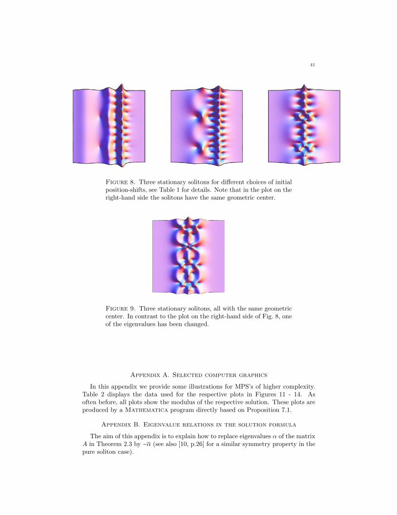
41
Figure 8. Three stationary solitons for different choices of initialposition-shifts, see Table 1 for details. Note that in the plot on theright-hand side the solitons have the same geometric center.
Figure 9. Three stationary solitons, all with the same geometriccenter. In contrast to the plot on the right-hand side of Fig. 8, oneof the eigenvalues has been changed.
Appendix A. Selected computer graphics
In this appendix we provide some illustrations for MPS’s of higher complexity.Table 2 displays the data used for the respective plots in Figures 11 - 14. Asoften before, all plots show the modulus of the respective solution. These plots areproduced by a Mathematica program directly based on Proposition 7.1.
Appendix B. Eigenvalue relations in the solution formula
The aim of this appendix is to explain how to replace eigenvalues α of the matrixA in Theorem 2.3 by −α (see also [10, p.26] for a similar symmetry property in thepure soliton case).
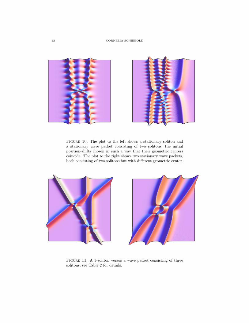
42 CORNELIA SCHIEBOLD
Figure 10. The plot to the left shows a stationary soliton anda stationary wave packet consisting of two solitons, the initialposition-shifts chosen in such a way that their geometric centerscoincide. The plot to the right shows two stationary wave packets,both consisting of two solitons but with different geometric center.
Figure 11. A 3-soliton versus a wave packet consisting of threesolitons, see Table 2 for details.

43
Figure 12. Collisions of two solitons with a wave packet consist-ing of two solitons.
Figure 13. Collisions of two wave packets, both consisting of two solitons.
Lemma B.1. Let Assumptions 3.1 and 3.2 be satisfied, and let Ak1 , Ak2 be Jordanblocks with the same eigenvalue αk1 = αk2 and with size nk1 ≤ nk2 . Then the solution
given in Theorem 2.3 is not altered if we simultaneously replace A by A and a, cby a, c, where
a) A is the matrix obtained from A by deleting the block Ak1 ,

44 CORNELIA SCHIEBOLD
Figure 14. Collisions of a soliton with a wave packet consistingof three solitons.
b) a, c are vectors obtained from a, c by replacing ak2 , ck2 by ak2 , ck2 appro-priately and deleting ak1 , ck1 .
In the proof we will specify how to choose ak2 , ck2 .
Proof. We may assume k1 = 1, k2 = 2, and that the solution is in reduced form, seeProposition 7.1. Define the n1 ×n2-matrix Π, the (n1 +n2)×n2-matrix Φ, and then × (n − n1)-matrix Ψ by
Π = (In1 0) , Φ = ( ΠIn2
) , Ψ = (Φ 00 In−n1
) .
For the Tij as in Proposition 7.1 we observe that T1j = ΠT2j for j ≥ 2, Ti1 = Ti2Πtr
for i ≥ 2, and T11 = ΠT22Πtr . Hence
(T11 T12
T21 T22) = (ΠT22Πtr ΠT22
T22Πtr T22) = ΦT22Φtr
and
(T1j
T2j) = (ΠT2j
T2j) = ΦT2j , (Ti1 Ti2) = (Ti2Πtr
Ti2) = Ti2Φtr
for i, j ≥ 2. This shows T = ΨTΨtr , where T = (Tij)Ni,j=2, and similarly one obtains
ff tr = Ψf f trΨtr , where f = (e(1)nj )Nj=2. As a result,
P = det (I + (M 0
0 M)(Ψ 0
0 Ψ)(−f f
tr −TT 0
)(Ψtr 00 Ψtr))
= det (I + (M 0
0 M)(−f f
tr −TT 0
)),

45
number ofeigenvalues
eigenvalues multiplicitiesvector encodinginitial shifts
plotted region
Fig. 11, N = 3 α1 = 1 n1 = 1 b1 = 2e−1 −20 ≤ x ≤ 20
left α2 = 1.5 + 0.2i n2 = 1 b2 = 3e10 −40 ≤ t ≤ 20
α3 = 0.9 − 0.4i n3 = 1 b3 = 4
Fig. 11, N = 3 α1 = 1 − 0.1i n1 = 3 b1 = (600,12,8) −20 ≤ x ≤ 20
right −50 ≤ t ≤ 50
Fig. 12, N = 3 α1 = 0.7 + 0.7i n1 = 1 b1 = 3e30 −15 ≤ x ≤ 25
left α2 = 0.5 − 0.2i n2 = 1 b2 = e−3 −60 ≤ t ≤ 20
α3 = 1 + 0.1i n3 = 2 b3 = (0,2)Fig. 12, N = 3 α1 = 0.5 − 0.7i n1 = 1 b1 = e20 −20 ≤ x ≤ 20
right α2 = 1.5 + 0.2i n2 = 1 b2 = 3e10 −50 ≤ t ≤ 50
α3 = 1 n3 = 2 b3 = (0,2)Fig. 13 N = 2 α1 = 1 n1 = 2 b1 = (6,1)e6 −25 ≤ x ≤ 35
left α2 = 0.5 − 0.5i n2 = 2 b2 = (−6,1)e−4 −20 ≤ t ≤ 40
Fig. 13 N = 2 α1 = 0.5 + 0.4i n1 = 2 b1 = (−20,1)e−10 −30 ≤ x ≤ 40
right α2 = 0.5 − 0.4i n2 = 2 b2 = (10,1)e5 −30 ≤ t ≤ 40
Fig. 14 N = 2 α1 = 1 − i n2 = 1 b1 = 2e30 −20 ≤ x ≤ 20
left α2 = 0.5 n1 = 3 b2 = (3,3,1) −15 ≤ t ≤ 35
Fig. 14 N = 2 α1 = 1 + 0.5i n2 = 1 b1 = 2e−10 −20 ≤ x ≤ 20
right α2 = 1 − 0.5i n1 = 3 b2 = (6,12,8) −20 ≤ t ≤ 10
Table 2. Summary of the data for the visualizations in Fig. 11-14.
where M = ΨtrMΨ. Furthermore, we get M = diagM2,M3, . . . ,MN, and M2 =ΦtrdiagM1,M2Φ =M2 +ΠtrM1Π.
Setting b(µ)1 = 0 for µ > n1, we can write
M2 =⎛⎜⎜⎝
m(1)2 m
(n2)2
⋰m(n2)2
⎞⎟⎟⎠
for m(µ)2 = ∑n2−(µ−1)
κ=1 (b(µ−1+κ)1 + b(µ−1+κ)
2 ) 1(κ−1)!
∂κ−1∂ακ−1 e
αx−iα2t.
The analogous reformulation holds for p. This shows that q = 1−P /p is not alteredif we delete the rows/columns corresponding to the first block and, simultaneously,
replace b(µ)2 by b
(µ)2 = b(µ)1 + b(µ)2 for µ ≤ n1.
Finally we explain how to choose a2, c2 appropriately. Set a(µ)2 = 1 for µ ≤ n2
and c(µ)2 = b(µ)2 − b(µ+1)
2 for µ < n2, c(n2)2 = b(n2)
2 . Then
n2−µ+1
∑κ=1
a(κ)2 c
(κ+µ−1)2 =
n2
∑λ=µ
c(λ)2 = b(µ)2 ,
in other words a2, c2 are related to b2 as in Proposition 7.1.
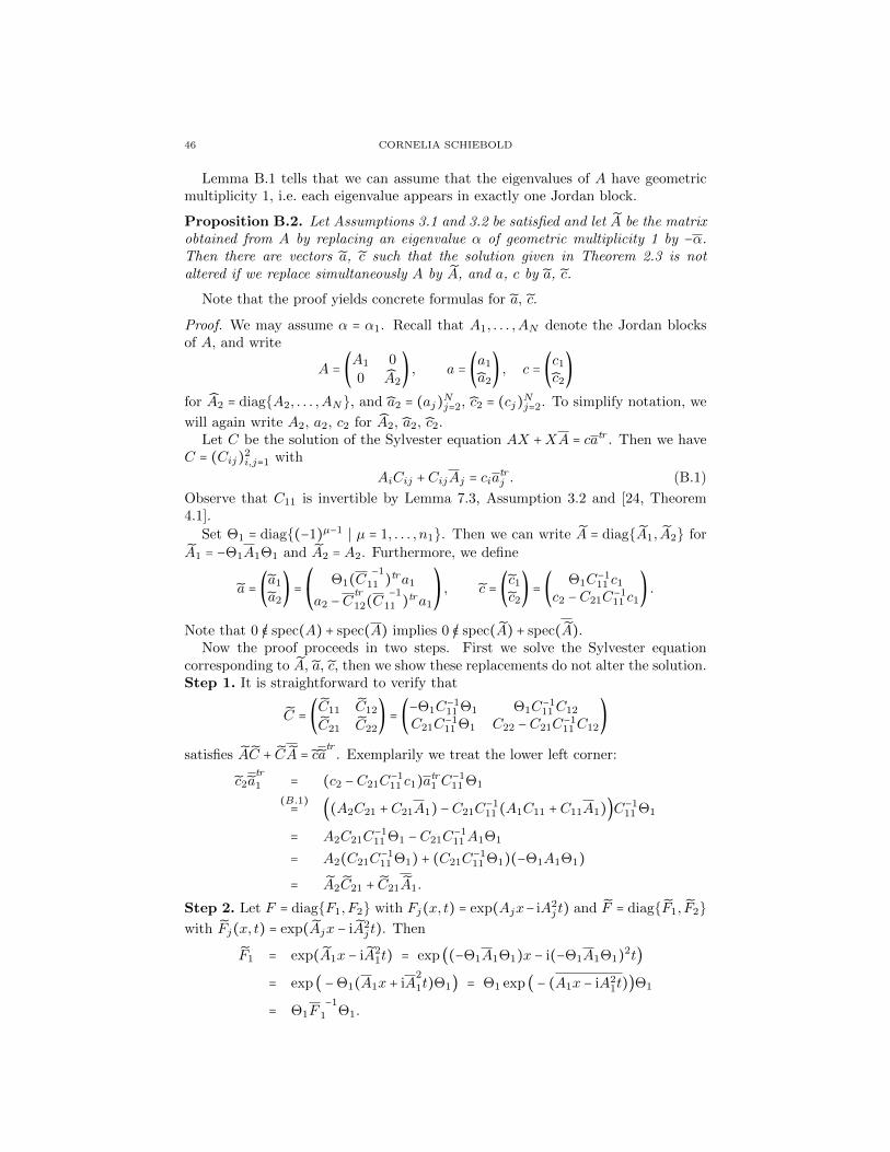
46 CORNELIA SCHIEBOLD
Lemma B.1 tells that we can assume that the eigenvalues of A have geometricmultiplicity 1, i.e. each eigenvalue appears in exactly one Jordan block.
Proposition B.2. Let Assumptions 3.1 and 3.2 be satisfied and let A be the matrixobtained from A by replacing an eigenvalue α of geometric multiplicity 1 by −α.Then there are vectors a, c such that the solution given in Theorem 2.3 is notaltered if we replace simultaneously A by A, and a, c by a, c.
Note that the proof yields concrete formulas for a, c.
Proof. We may assume α = α1. Recall that A1, . . . ,AN denote the Jordan blocksof A, and write
A = (A1 0
0 A2) , a = (a1
a2) , c = (c1
c2)
for A2 = diagA2, . . . ,AN, and a2 = (aj)Nj=2, c2 = (cj)Nj=2. To simplify notation, we
will again write A2, a2, c2 for A2, a2, c2.Let C be the solution of the Sylvester equation AX +XA = catr . Then we have
C = (Cij)2i,j=1 with
AiCij +CijAj = ciatrj . (B.1)
Observe that C11 is invertible by Lemma 7.3, Assumption 3.2 and [24, Theorem4.1].
Set Θ1 = diag(−1)µ−1 ∣ µ = 1, . . . , n1. Then we can write A = diagA1, A2 for
A1 = −Θ1A1Θ1 and A2 = A2. Furthermore, we define
a = (a1
a2) =
⎛⎝
Θ1(C−1
11 )tra1
a2 −Ctr
12(C−1
11 )tra1
⎞⎠, c = (c1
c2) = ( Θ1C
−111 c1
c2 −C21C−111 c1
) .
Note that 0 /∈ spec(A) + spec(A) implies 0 /∈ spec(A) + spec(A).Now the proof proceeds in two steps. First we solve the Sylvester equation
corresponding to A, a, c, then we show these replacements do not alter the solution.Step 1. It is straightforward to verify that
C = (C11 C12
C21 C22) = (−Θ1C
−111 Θ1 Θ1C
−111C12
C21C−111 Θ1 C22 −C21C
−111C12
)
satisfies AC + CA = catr . Exemplarily we treat the lower left corner:
c2atr
1 = (c2 −C21C−111 c1)atr1 C−1
11 Θ1
(B.1)= ((A2C21 +C21A1) −C21C−111 (A1C11 +C11A1))C−1
11 Θ1
= A2C21C−111 Θ1 −C21C
−111A1Θ1
= A2(C21C−111 Θ1) + (C21C
−111 Θ1)(−Θ1A1Θ1)
= A2C21 + C21A1.
Step 2. Let F = diagF1, F2 with Fj(x, t) = exp(Ajx− iA2j t) and F = diagF1, F2
with Fj(x, t) = exp(Ajx − iA2j t). Then
F1 = exp(A1x − iA21t) = exp ((−Θ1A1Θ1)x − i(−Θ1A1Θ1)2t)
= exp ( −Θ1(A1x + iA2
1t)Θ1) = Θ1 exp ( − (A1x − iA21t))Θ1
= Θ1F−1
1 Θ1.
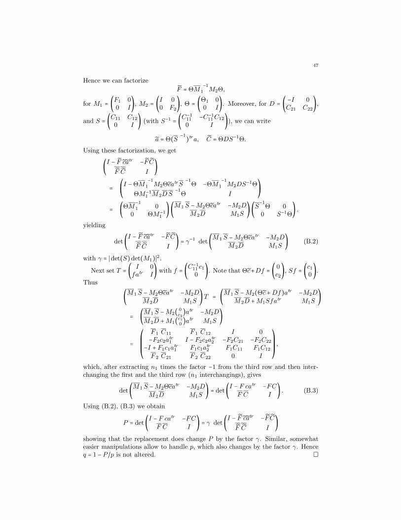
47
Hence we can factorize
F = ΘM−1
1 M2Θ,
for M1 = (F1 00 I
), M2 = (I 00 F2
), Θ = (Θ1 00 I
). Moreover, for D = ( −I 0C21 C22
),
and S = (C11 C12
0 I) (with S−1 = (C
−111 −C−1
11C12
0 I)), we can write
a = Θ(S −1)tra, C = ΘDS−1Θ.
Using these factorization, we get
(I − F catr −F CF C I
)
=⎛⎝I −ΘM
−1
1 M2ΘcatrS−1
Θ −ΘM−1
1 M2DS−1Θ
ΘM−11 M2DS
−1Θ I
⎞⎠
= (ΘM−1
1 00 ΘM−1
1
)(M1 S −M2Θcatr −M2D
M2D M1S)(S
−1Θ 0
0 S−1Θ) .
yielding
det(I − F catr −F CF C I
) = γ−1 det(M1 S −M2Θcatr −M2D
M2D M1S) (B.2)
with γ = ∣det(S)det(M1)∣2.
Next set T = ( I 0fatr I
) with f = (C−111 c10
). Note that Θc+Df = ( 0c2
), Sf = (c10).
Thus
(M1 S −M2Θcatr −M2D
M2D M1S)T = (M1 S −M2(Θc +Df)atr −M2D
M2D +M1Sfatr M1S
)
= (M1 S −M2( 0c2)atr −M2D
M2D +M1(c10 )atr M1S
)
=⎛⎜⎜⎜⎝
F 1 C11 F 1 C12 I 0−F2c2a
tr1 I − F2c2a
tr2 −F2C21 −F2C22
−I + F1c1atr1 F1c1a
tr2 F1C11 F1C12
F 2 C21 F 2 C22 0 I
⎞⎟⎟⎟⎠,
which, after extracting n1 times the factor −1 from the third row and then inter-changing the first and the third row (n1 interchangings), gives
det(M1 S −M2Θcatr −M2D
M2D M1S) = det(I − F ca
tr −FCF C I
) . (B.3)
Using (B.2), (B.3) we obtain
P = det(I − F catr −FC
F C I) = γ det(
I − F catr −F CF C I
)
showing that the replacement does change P by the factor γ. Similar, somewhateasier manipulations allow to handle p, which also changes by the factor γ. Henceq = 1 − P /p is not altered.

48 CORNELIA SCHIEBOLD
Appendix C. Global regularity
In this appendix we complete the proof of Theorem 2.3. Recall that we havealready obtained a solution on Ω = (x, t) ∣ I + LL is invertible. Hence it suffices
to show that det(I +LL) /= 0 holds for every (x, t) ∈ R. The main ingredient of theproof is the following factorization result for solutions of the Sylvester equation.
Proposition C.1. Let Assumptions 3.1 and 3.2 be met, and suppose Re(αj) > 0for all j. Let ϕ, ψ be polynomials of one complex variable z satisfying
1
(ν − 1)!∂ν−1
∂zν−1∣z=αj
eϕ(z) = c(nj−ν+1)j ,
1
(ν − 1)!∂ν−1
∂zν−1∣z=αj
eψ(z) = a(ν)j ,
for ν = 1, . . . , nj, j = 1, . . . ,N . Moreover, set ϕ(z) = ϕ(z), ψ(z) = ψ(z).
Denote by ejν ∈ Cn =⊕Nj=1 Cnj the vector which is the νth standard basis vector
on the component Cnj and the zero-vector on all other components. Define theoperators T ∶ Cn Ð→ L2(−∞,0] and S ∶ L2(−∞,0]Ð→ Cn by
Tejν = fjν , Sf =N
∑j=1
nj
∑ν=1
sjν(f)ejν ,
where
fjν(σ) = 1
(ν − 1)!∂ν−1
∂zν−1∣z=αj
ezσ+ψ(z),
sjν(f) =0
∫−∞
f(s) 1
(nj − ν)!∂nj−ν
∂znj−ν∣z=αj
ezs+ϕ(z)ds,
and the analogous operators S, T which are obtained by replacing ψ, ϕ with ψ, ϕ,respectively, and αj with αj.
Finally, let C ∈ L(Cn) be the solution of the Sylvester equation AX +XA = catr ,and let K ∈ L(L2(−∞,0]) be the integral operator3 with kernel
k(σ, s) =N
∑j=1
1
(nj − 1)!∂nj−1
∂znj−1∣z=αj
e(σ+s)z+ϕ(z)+ψ(z).
Then,
a) K = TS,
b) C = ST ,
c) CC is related4 to the integral operator H with kernel
h(σ, s) = ∫0
−∞k(σ, ρ) k(ρ, s) dρ,
which is self-adjoint and positive.
Note that Assumption 3.2 guarantees the existence of ϕ and ψ.
3 i.e. (Kf)(σ) = ∫0
−∞k(σ, s)f(s)ds
4 Two operators S ∈ L(E), T ∈ L(F ), where E, F are complex Banach spaces, are called relatedif there exist A ∈ L(E,F ) and B ∈ L(F,E) such that S = BA and T = AB.
49
Proof. In the sequel, we will consider variations of the integral kernels with respectto a parameter z close to αj . Since Re(αj) > 0, we may assume Re(z) ≥ ε for someε > 0.
a) Observe that
sjν(f) = ∫0
−∞gjν(s)f(s)ds for gjν(s) =
1
(nj − ν)!∂nj−ν
∂znj−ν∣z=αj
ezs+ϕ(z).
Hence,
(TSf)(σ) =N
∑j=1
nj
∑ν=1
sjν(f)fjν(σ) =0
∫−∞
(N
∑j=1
nj
∑ν=1
gjν(s)fjν(σ))f(s)ds,
showing that TS is the integral operator with kernel
k(σ, s) =N
∑j=1
nj
∑ν=1
gjν(s)fjν(σ)
=N
∑j=1
1
(nj − 1)!
nj
∑ν=1
(nj − 1
ν − 1)( ∂nj−ν
∂znj−ν∣z=αj
ezs+ϕ(z))( ∂ν−1
∂zν−1∣z=αj
ezσ+ψ(z))
=N
∑j=1
1
(nj − 1)!∂nj−1
∂znj−1∣z=αj
e(s+σ)z+ϕ(z)+ψ(z).
b) Let fjν be the analogous function to fjν which is obtained by replacing ψ by
ψ and αj by αj . Then we obtain
⟨ST ejν , eiµ⟩ = siµ(T ejν) = ∫0
−∞giµ(s)fjν(s)ds
= 1
(ni − µ)!∂ni−µ
∂wni−µ∣w=αi
1
(ν − 1)!∂ν−1
∂zν−1∣z=αj
eϕ(w)+ψ(z)
w + z . (C.1)
From the definition of the polynomial ψ, we have 1κ!
∂κ
∂zκ∣z=αj
eψ(z) = a(κ+1)j , hence a
direct application of the Leibnitz rule yields
1
(ν − 1)!∂ν−1
∂zν−1∣z=αj
1
w + z eψ(z) =
ν−1
∑ν′=0
(−1)ν′( 1
w + αj)ν′+1
a(ν−ν′)j . (C.2)
Furthermore, again from the Leibnitz rule,
1
(ni − µ)!∂ni−µ
∂wni−µ∣w=αi
( 1
w + αj)ν′+1
eϕ(w)
=ni−µ∑µ′=0
(−1)µ′(µ
′ + ν′µ′
)( 1
αi + αj)µ′+ν′+1
c(µ+µ′)i , (C.3)
Inserting (C.2), (C.3) into (C.1) and substituting summation indices µ′, ν′ withµ′ + 1, ν′ + 1, respectively, we obtain as result
⟨ST ejν , eiµ⟩ =ni−µ+1
∑µ′=1
ν
∑ν′=1
(−1)µ′+ν′a
(ν−(ν′−1))j c
(µ+(µ′−1))i (µ
′ + ν′ − 2
µ′ − 1)( 1
αi + αj)µ′+ν′−1
.
Finally, comparison with Lemma 7.3 shows that ⟨ST ejν , eiµ⟩ coincides with theµνth entry of Cij .

50 CORNELIA SCHIEBOLD
c) As in b) one shows C = ST . The factorization CC = (ST S)T then tells us
that CC and H = T (ST S) are related operators. As in a), one verifies that T S isthe integral operator with kernel
k(σ, s) =N
∑j=1
1
(nj − 1)!∂nj−1
∂znj−1∣z=αj
e(s+σ)z+ϕ(z)+ψ(z).
Moreover,
k(σ, s) = k(σ, s)from the definitions of ϕ, ψ. Now it is straightforward to check that H = (TS)(T S)is the integral operator with the kernel h(σ, s) as claimed.
Observe k(σ, s) = k(s, σ). Hence h(s, σ) = h(σ, s), implying (Hg, f) = (g,Hf)for all f , g ∈ L2(−∞,0]. Together with the fact that H is bounded, it follows thatH is self-adjoint. To show that H is positive, we finally check
(Hf, f) = ∫0
−∞∫
0
−∞h(σ, s)f(s)ds f(σ)dσ
= ∫0
−∞(∫
0
−∞k(ρ, s)f(s)ds)(∫
0
−∞k(σ, ρ)f(σ)dσ)dρ
= ∫0
−∞∣ ∫
0
−∞k(ρ, s)f(s)ds ∣
2
≥ 0
for all f ∈ L2(−∞,0]. This completes the proof.
Second part of the proof of Theorem 2.3. According to Section 5 we may assumethat Assumptions 3.1 and 3.2 are met. Furthermore, we may assume Re(αj) > 0for all j according to Appendix B.
Observe that L = L(x, t) = eAx−iA2tC satisfies the (x, t)-dependent Sylvester
equation AL(x, t) +L(x, t)A = c(x, t) atr for the vector-function c(x, t) = eAx−iA2tc.
By Proposition C.1 c), LL is related to an integral operator on L2(−∞,0] which ispositive and therefore has non-negative eigenvalues. From the principle of relatedoperators [16] it follows that also LL has only non-negative eigenvalues. Hence
p = det( I −LL I
) (2.7)= det (I +LL) ≥ 1.
References
[1] M.J. Ablowitz, B. Prinari, and A.D. Trubatch. ‘Discrete and Continuous NonlinearSchrodinger Systems.’ Cambridge University Press, Cambridge, 2003.
[2] M.J. Ablowitz, D.J. Kaup, A.C. Newell, and H. Segur. The inverse scattering transform
Fourier analysis for nonlinear problems. Stud. Appl. Math. 53 (1974), 249-315.[3] M.J. Ablowitz and H. Segur. ‘Solitons and the Inverse Scattering Transform.’ SIAM, Philadel-
phia, 1981
[4] H. Aden and B. Carl. On realizations of solutions of the KdV equation by determinants onoperator ideals. J. Math. Phys. 37 (1996), 1833–1857.
[5] T. Aktosun, F. Demontis, and C. van der Mee. Exact solutions to the focusing nonlinearSchrodinger equation Inverse Problems 23 (2007), 2171-2195.
[6] H. Blohm. Solution of nonlinear equations by trace methods. Nonlinearity 13 (2000), 1925–
1964.[7] B. Carl and S.Z. Huang. On realizations of solutions of the KdV equation by the C0-semigroup
method. Amer. J. Math. 122 (2000), 403–438.
51
[8] B. Carl and C. Schiebold. Nonlinear equations in soliton physics and operator ideals. Non-
linearity 12 (1999), 333–364.
[9] B. Carl and C. Schiebold. Ein direkter Ansatz zur Untersuchung von Solitonengleichungen.Jahresber. Deutsch. Math.-Verein. 102 (2000), 102–148.
[10] A. Dimakis and F. Muller-Hoissen Solutions of matrix NLS systems and their discretisations:
A unified treatment Inverse Problems 26 (2010), 095007.[11] W. Eckhaus and A. van Harten. ‘The Inverse Scattering Transformation and The Theory of
Solitons.’ Mathematics Studies 50, North-Holland Publishing Company, Amsterdam 1981.
[12] B. Fuchssteiner and R.N. Aiyer. Multisolitons, or the discrete eigenfunctions of the recursionoperator on non-linear evolution equations: II. Background. J. Phys. A 20 (1987), 375–388.
[13] C.S. Gardner, J.M. Greene, M.D. Kruskal, and R.M. Miura. Method for solving the Korteweg-
de Vries equation. Phys. Rev. Lett. 19 (1967), 1095-1097.[14] V.A. Marchenko. ‘Nonlinear Equations and Operator Algebras.’ Reidel, Dordrecht, 1988.
[15] E. Olmedilla. Multiple pole solutions of the non-linear Schrodinger equation. Physica D 25(1986), 330–346.
[16] A. Pietsch. ‘Eigenvalues and s-Numbers.’ Cambridge University Press, Cambridge 1987.
[17] C. Poppe. Construction of solutions of the sine-Gordon equation by means of Fredholmdeterminants. Physica D 9 (1983), 103–139.
[18] A. L. Sakhnovich Non-self-adjoint Dirac-type systems and related nonlinear equations: wave
functions, solutions, and explicit formulas. Integral Equations Operator Theory 55 (2006),127–143.
[19] C. Schiebold. Solitons of the sine-Gordon equation coming in clusters. Revista Matematica
Complutense 15 (2002), 265–325.[20] C. Schiebold. On negatons of the Toda lattice. J. Nonlin. Math. Phys. 10 (2003), 181–193.
[21] C. Schiebold. ‘Integrable Systems and Operator Equations.’ Habilitation thesis, Jena Univer-
sity, 2004 (http://apachepersonal.miun.se/˜corsch/Habilitation.PDF).[22] C. Schiebold, A non-abelian Nonlinear Schrodinger equation and countable superposition of
solitons. J. Gen. Lie Theory Appl. 2 (2008), 245–250.[23] C. Schiebold. Noncommutative AKNS systems and multisoliton solutions to the matrix sine-
Gordon equation. Discrete and Continuous Dynamical Sytems, Supplement 2009 (2009), 678-
690.[24] C. Schiebold. Cauchy-type determinants and integrable systems. Linear Algebra Appl. 433
(2010), 447–475.
[25] C. Schiebold. The noncommutative AKNS system: projection to matrix systems, countablesuperposition and soliton-like solutions . J. Phys. A 43 (2010), 434030.
[26] J.J. Sylvester. Sur l’equation en matrices px = xq. C. R. Acad. Sci. Paris 99 (1884) 67-71,
115-116.[27] S. Tanaka. Non-linear Schrodinger equation and modified Korteweg-de Vries equation; Con-
struction of solutions in terms of scattering data. Publ. RIMS Kyoto Univ. 10 (1975), 329–
357.[28] H. Tsuru and M. Wadati. The multiple pole solutions of the sine-Gordon equation. J. Phys.
Soc. Japan 9 (1984), 2908–2921.[29] M. Wadati and K. Ohkuma. Multiple pole solutions of the modified Korteweg-de Vries equa-
tion. J. Phys. Soc. Japan 51 (1981), 2029–2035.
[30] V.E. Zakharov and A. Shabat. Exact theory of two-dimensional self-focusing and one-dimensional self-modulation of waves in nonlinear media Sov. Phys. JETP 34 (1972), 62–69.
E-mail address: [email protected]