APPLICATIONS OF COMPRESSED SENSING TO MAGNETIC RESONANCE IMAGING

Speaker: Lingling Pu

Acknowledgements2

Ali Bilgin, Ted Trouard, Maria Altbach, Yookyung Kim, Lee RyanDepartment of Biomedical Engineering, University of Arizona, Tucson, AZ

Department of Radiology, University of Arizona, Tucson, AZ

Department of Electrical and Computer Engineering, University of Arizona, Tucson, AZ

Department of Psychology, University of Arizona, Tucson, AZ

Onur GuleryuzDepartment of Electrical Engineering, Polytechnic Institute of NYU, Brooklyn, NY

Mariappan NadarSiemens Corporation, Corporate Research, Princeton, NJ

Outline

Wavelet Information Assisted Model-based CS Reconstruction

SPArse Reconstruction using a ColLEction of bases (SPARCLE)

Voxel-based Morphometry Study Based on SPARCLE-CS Reconstructed T1-weighted images

3

Compressed Sensing

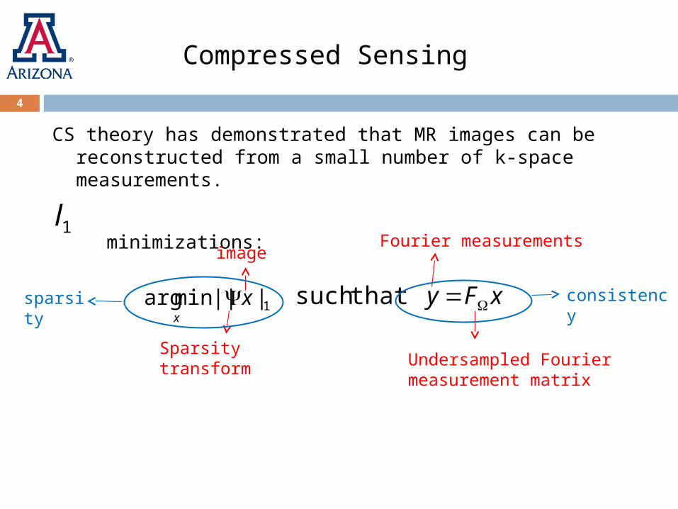
CS theory has demonstrated that MR images can be reconstructed from a small number of k-space measurements.

minimizations:

4

1l

1||||minarg xx

xFy thatsuch

Sparsity transform

image

Undersampled Fouriermeasurement matrix

Fourier measurements

consistencysparsity

Selection of Sparsity Basis

Two considerations for selection of the sparsity transform Ψ

Sparse signal representation

Incoherency with measurement basis

Ex: Orthonormal wavelet transformsUsually no strong preference to select a particular wavelet basis.

Many wavelets yield qualitatively and quantitatively similar reconstructions.

5

Selection of Sparsity Basis

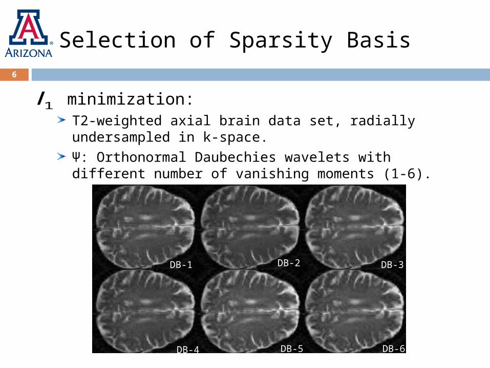
minimization:T2-weighted axial brain data set, radially undersampled in k-space.

Ψ: Orthonormal Daubechies wavelets with different number of vanishing moments (1-6).

DB-1 DB-2 DB-3

DB-4 DB-5 DB-6

1l

6

Selection of Sparsity Basis

Question: Can we somehow benefit from the fact that the reconstruction artifacts are (slightly) different in different bases?

DB-1 DB-2

DB-4 DB-5 DB-6

DB-3 Observations:

•Qualitatively no significant difference between reconstructions.

•Reconstruction artifacts are slightly different.

7

SPArse Reconstruction using a ColLEction of bases (SPARCLE)†

8

Incoherencebetween Ψ and FΩ

Undersampling artifacts accumulate incoherently

in Ψ

Small coefficients

in Ψ

Our approach: Enforce sparsity in a collection of bases Ψi , i=1,…,N

Each basis Ψi provides a sparse representation.

In addition, the undersampling artifacts are different in each basis.

A large coefficient due to undersampling artifacts in one basis is likely to result in small coefficients in the other basis.

By requiring that the result be sparse in multiple bases, a significantly larger portion of the undersampling artifacts can be removed.

†: A. Bilgin et al, “SPArse Reconstruction using a ColLEction of bases (SPARCLE),” in Proc. of 2009 Meeting of ISMRM, 2009.

SPArse Reconstruction using a ColLEction of bases (SPARCLE)†

9

Measurement Space (Fourier)

Sparsity Space Ψ1

Project

ProjectThreshold to remove small coefficients

Assert consistencywith measured data

Sparsity Space Ψ2

Project

Repeat for the next Sparsity basis

Results10

Radial-FSE dataset (TR=4.5s, FOV=26cm and ETL=4, 256x256 acquisition) retrospectively subsampled to 64 radial views

Original l1-min DB6 SPARCLE

Outline

Wavelet Information Assisted Model-based CS Reconstruction

SPArse Reconstruction using a ColLEction of bases (SPARCLE)

Voxel-based Morphometry Study Based on SPARCLE-CS Reconstructed T1-weighted images

11

Motivation

CS assumes that transform coefficients are independent

Correlation between wavelet coefficients

→ We exploit statistical dependencies of the wavelet coefficients by modeling them as Gaussian Scale Mixture (GSM) in the CS framework

12

Statistics in Wavelet Domain

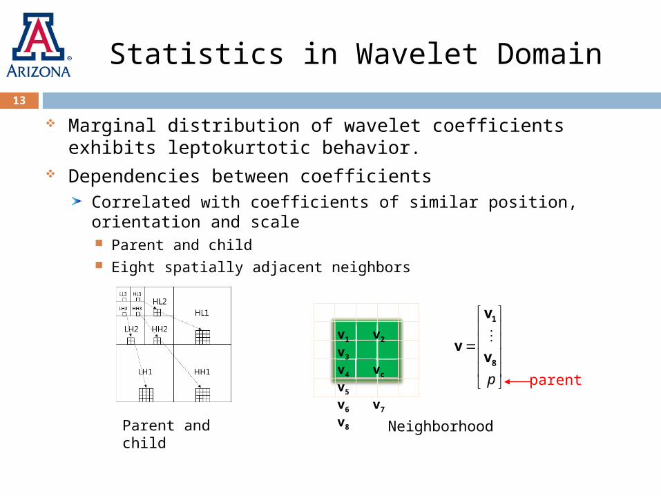
Marginal distribution of wavelet coefficients exhibits leptokurtotic behavior.

Dependencies between coefficientsCorrelated with coefficients of similar position, orientation and scale Parent and child Eight spatially adjacent neighbors

Parent and child

Neighborhood

13

p

1

8

v

vv

parent

v1 v2 v3

v4 vc v5

v6 v7 v8

Bayes Least Squares-Gaussian Scale Mixtures†(BLS-GSM)

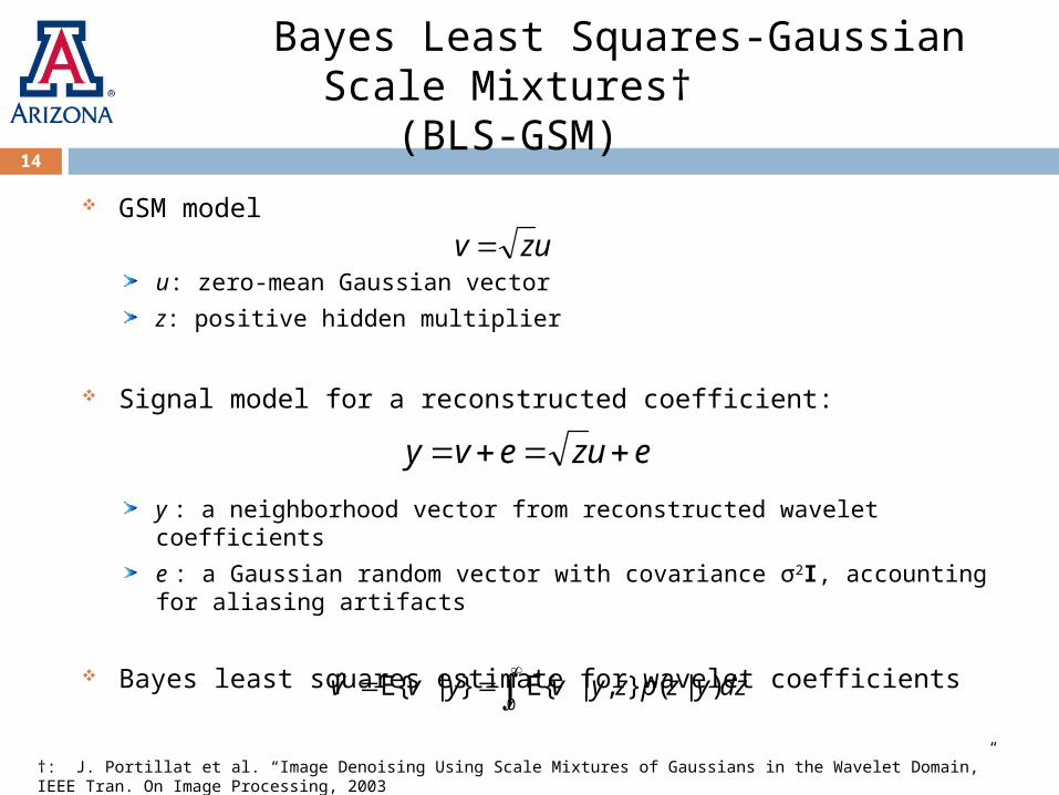
GSM model

u: zero-mean Gaussian vector

z: positive hidden multiplier

Signal model for a reconstructed coefficient:

y : a neighborhood vector from reconstructed wavelet coefficients

e : a Gaussian random vector with covariance σ2I, accounting for aliasing artifacts

Bayes least squares estimate for wavelet coefficients

14

dzyzpzyvyvv )|(},|{E}|{Eˆ0

euzevy

†: J. Portillat et al. “Image Denoising Using Scale Mixtures of Gaussians in the Wavelet Domain,” IEEE Tran. On Image Processing, 2003

uzv

Iterative Hard Thresholding (IHT) †

IHTMo-Sparse problem

Solved by the iterative algorithm

where HMo is the element-wise hard thresholding operator that retains the Mo largest coefficients

BLS-GSM IHTIHT is used to generate signal estimates

BLS-GSM model is imposed to re-estimate the signal

Impose Mo sparsity

2

2 0min s.t. oM xb Ax x

1 ( ( ))o

n n H nMH x x A b Ax

†: T. Blumensath, M. E. Davies, "Normalised Iterative Hard Thresholding; guaranteed stability and performance.” 2009.

15

Results16

Original 100V

BLS-GSM IHT IHT

17.58 dB

20.87 dB23.88 dB

Test images: T2-weighted radial-FSE (256 radial views x 256 points )

Results

2.59 dB improvement on average

60 80 100 120 140 160 180 200 22015

20

25

30

Views

SN

R (

dB)

Brain

IHT

BLS-GSM IHT

17

60 80 100 120 140 160 180 200 2200

100

200

300

400

500

600

Views

Iter

atio

nsBrain

IHT

BLS-GSM IHT

Results18

Outline

Wavelet Information Assisted Model-based CS Reconstruction

SPArse Reconstruction using a ColLEction of bases (SPARCLE)

Voxel-based Morphometry Study Based on SPARCLE-CS Reconstructed T1-weighted images

19

A Voxel-based Morphometry (VBM) Study†

20

VBM Investigates local differences in brain anatomy, after discounting the large-scale anatomical differences

Enables classical inferences about the regionally-specific effects

Participants69 females (ages 52-92 years) living independently, normal memory and executive function.

Two groups: Anti-inflammatory (AI) drug users Control (non-AI drug users)

InvestigateCorrelation between gray matter volume changes and age.

Identify brain regions where age-related volume decreases were significantly greater in one group compared to the other.

†: K. Walther et al, “Anti-inflammatory drugs reduce age-related decreases in brain volume in cognitively normal older adults,” in Neurobiology of Aging, 2009.

A Voxel-based Morphometry (VBM) Study

21

ImagesT1-weighted images of the whole brain with a section thickness of 0.7mm (TR = 5.1 ms, TE = 2 ms, TI = 500 ms; flip angle = 15◦; matrix = 256×256; FOV= 260mm×260 mm).

Image reconstructionsSPARCLE CS

General linear model (GLM) was used to carry out the multiple regression analysis.

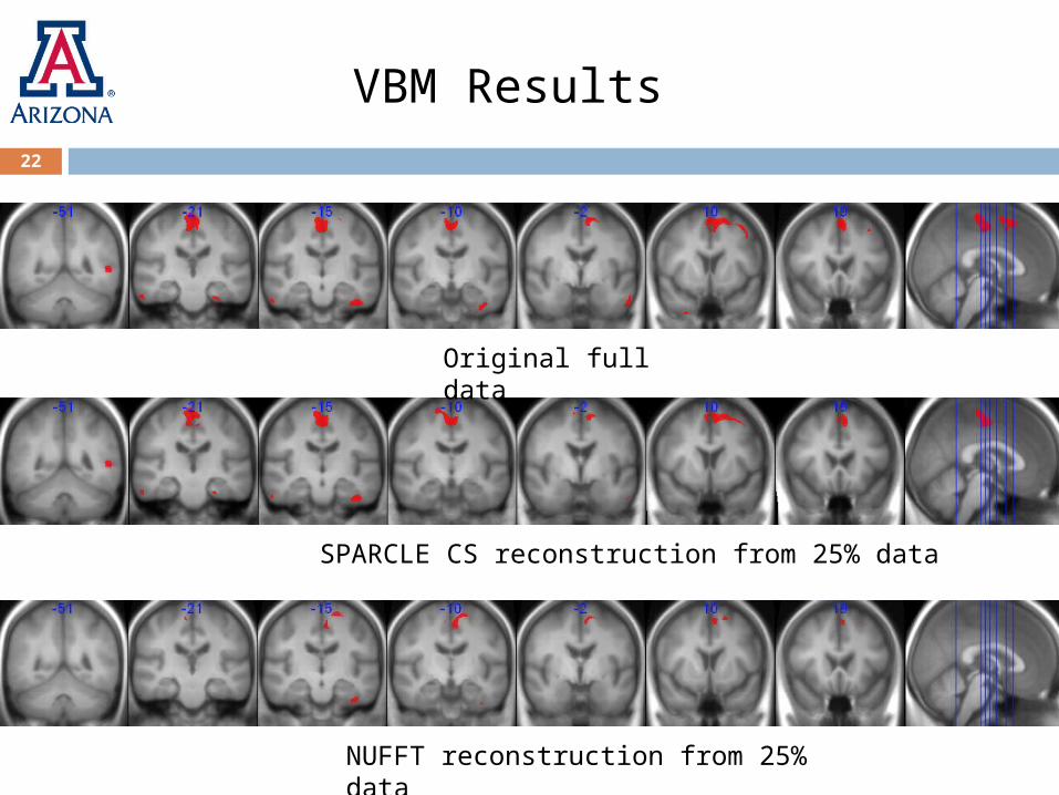
VBM Results22

Original full data

SPARCLE CS reconstruction from 25% data

NUFFT reconstruction from 25% data

VBM Results23

SPM result based on the original data.

Define Region-of-Interest (ROI):- centered at each of the peaked voxel - radius 10 mm sphere

VBM Results24

ROI 1

ROI 2

ROI 3

ROI 4

ROI 5

ROI 6

ROI 7

ROI 8

ROI 9

ROI 10

0.979

0.981

0.973

0.937

0.964

0.971

0.978

0.946

0.959

0.952

ROI 11

ROI 12

ROI 13

ROI 14

ROI 15

ROI 16

ROI 17

ROI 18

ROI 19

mean

0.856

0.954

0.957

0.958

0.918

0.969

0.980

0.963

0.961

0.956

)( 2R Correlation coefficients