Embed Size (px)
Citation preview

Compressed Sensing - beyond the ShannonParadigm
Wolfgang Dahmen
Institut fur Geometrie und Praktische MathematikRWTH Aachen
joint work with Albert Cohen and Ron DeVore
ISWCS-11, Aachen, Nov.8, 2011
W. Dahmen (RWTH Aachen) Compressed Sensing 28.10.2011 1 / 30

Contents
1 Motivation, Background
2 A New Paradigm
3 Back to the 70’s - An Information Theoretic Bound
4 Randomness Helps...
5 An Optimal Decoder
6 Electron-Tomography
W. Dahmen (RWTH Aachen) Compressed Sensing 28.10.2011 2 / 30

Contents
1 Motivation, Background
2 A New Paradigm
3 Back to the 70’s - An Information Theoretic Bound
4 Randomness Helps...
5 An Optimal Decoder
6 Electron-Tomography
W. Dahmen (RWTH Aachen) Compressed Sensing 28.10.2011 2 / 30

Contents
1 Motivation, Background
2 A New Paradigm
3 Back to the 70’s - An Information Theoretic Bound
4 Randomness Helps...
5 An Optimal Decoder
6 Electron-Tomography
W. Dahmen (RWTH Aachen) Compressed Sensing 28.10.2011 2 / 30

Contents
1 Motivation, Background
2 A New Paradigm
3 Back to the 70’s - An Information Theoretic Bound
4 Randomness Helps...
5 An Optimal Decoder
6 Electron-Tomography
W. Dahmen (RWTH Aachen) Compressed Sensing 28.10.2011 2 / 30

Contents
1 Motivation, Background
2 A New Paradigm
3 Back to the 70’s - An Information Theoretic Bound
4 Randomness Helps...
5 An Optimal Decoder
6 Electron-Tomography
W. Dahmen (RWTH Aachen) Compressed Sensing 28.10.2011 2 / 30

Contents
1 Motivation, Background
2 A New Paradigm
3 Back to the 70’s - An Information Theoretic Bound
4 Randomness Helps...
5 An Optimal Decoder
6 Electron-Tomography
W. Dahmen (RWTH Aachen) Compressed Sensing 28.10.2011 2 / 30

The Nyquist-Shannon Theorem
A bandlimited “signal” f (t), t ∈ R, with bandwidth 2B can bereconstructed exactly from the samples f (kτ), τ < 1/2B, ...
X (f )(ω) :=
∫R
f (t)e−i2πtωdt = 0, |ω| > B,
f (t) =∞∑
k=−∞f (kτ)
sinπ(τ−1t − k)
π(τ−1t − k)
W. Dahmen (RWTH Aachen) Compressed Sensing 28.10.2011 3 / 30

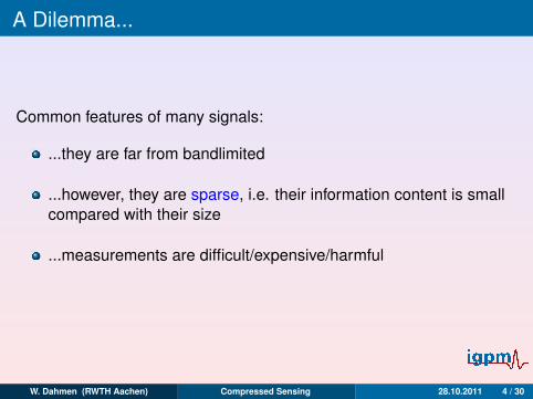
A Dilemma...
Common features of many signals:
...they are far from bandlimited
...however, they are sparse, i.e. their information content is smallcompared with their size
...measurements are difficult/expensive/harmful
W. Dahmen (RWTH Aachen) Compressed Sensing 28.10.2011 4 / 30

A Dilemma...
Common features of many signals:
...they are far from bandlimited
...however, they are sparse, i.e. their information content is smallcompared with their size
...measurements are difficult/expensive/harmful
W. Dahmen (RWTH Aachen) Compressed Sensing 28.10.2011 4 / 30

A Dilemma...
Common features of many signals:
...they are far from bandlimited
...however, they are sparse, i.e. their information content is smallcompared with their size
...measurements are difficult/expensive/harmful
W. Dahmen (RWTH Aachen) Compressed Sensing 28.10.2011 4 / 30
A Dilemma...
Common features of many signals:
...they are far from bandlimited
...however, they are sparse, i.e. their information content is smallcompared with their size
...measurements are difficult/expensive/harmful
W. Dahmen (RWTH Aachen) Compressed Sensing 28.10.2011 4 / 30
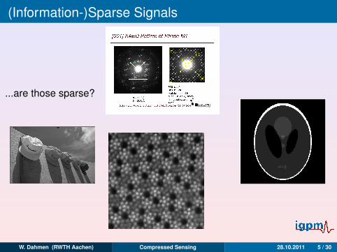
(Information-)Sparse Signals
...are those sparse?
W. Dahmen (RWTH Aachen) Compressed Sensing 28.10.2011 5 / 30

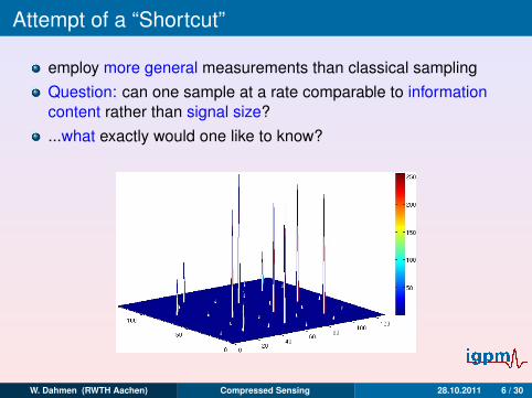
Attempt of a “Shortcut”
employ more general measurements than classical sampling
Question: can one sample at a rate comparable to informationcontent rather than signal size?...what exactly would one like to know?
W. Dahmen (RWTH Aachen) Compressed Sensing 28.10.2011 6 / 30

Attempt of a “Shortcut”
employ more general measurements than classical samplingQuestion: can one sample at a rate comparable to informationcontent rather than signal size?
...what exactly would one like to know?
W. Dahmen (RWTH Aachen) Compressed Sensing 28.10.2011 6 / 30

Attempt of a “Shortcut”
employ more general measurements than classical samplingQuestion: can one sample at a rate comparable to informationcontent rather than signal size?...what exactly would one like to know?
W. Dahmen (RWTH Aachen) Compressed Sensing 28.10.2011 6 / 30
Attempt of a “Shortcut”
employ more general measurements than classical samplingQuestion: can one sample at a rate comparable to informationcontent rather than signal size?...what exactly would one like to know?
W. Dahmen (RWTH Aachen) Compressed Sensing 28.10.2011 6 / 30

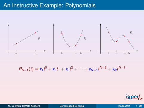
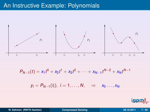
An Instructive Example: Polynomials
t1 t2
P1
t1 t2 t3
P2
t1 t4t2
P3
t3
PN−1(t) = x1t0 + x2t1 + x3t2 + · · ·+ xN−1tN−2 + xN tN−1
yi = PN−1(ti), i = 1, . . . ,N,
⇒ x0 . . . , xN
W. Dahmen (RWTH Aachen) Compressed Sensing 28.10.2011 7 / 30

An Instructive Example: Polynomials
t1 t2
P1
t1 t2 t3
P2
t1 t4t2
P3
t3
PN−1(t) = x1t0 + x2t1 + x3t2 + · · ·+ xN−1tN−2 + xN tN−1
yi = PN−1(ti), i = 1, . . . ,N,
⇒ x0 . . . , xN
W. Dahmen (RWTH Aachen) Compressed Sensing 28.10.2011 7 / 30

An Instructive Example: Polynomials
t1 t2
P1
t1 t2 t3
P2
t1 t4t2
P3
t3
PN−1(t) = x1t0 + x2t1 + x3t2 + · · ·+ xN−1tN−2 + xN tN−1
yi = PN−1(ti), i = 1, . . . ,N, ⇒ x0 . . . , xN
W. Dahmen (RWTH Aachen) Compressed Sensing 28.10.2011 7 / 30
An Instructive Example: Polynomials
t1 t2
P1
t1 t2 t3
P2
t1 t4t2
P3
t3
PN−1(t) = x1t0 + x2t1 + x3t2 + · · ·+ xN−1tN−2 + xN tN−1
yi = PN−1(ti), i = 1, . . . ,N, ⇒ x0 . . . , xN
W. Dahmen (RWTH Aachen) Compressed Sensing 28.10.2011 7 / 30
An Instructive Example: Polynomials
t1 t2
P1
t1 t2 t3
P2
t1 t4t2
P3
t3
PN−1(t) = x1t0 + x2t1 + x3t2 + · · ·+ xN−1tN−2 + xN tN−1
yi = PN−1(ti), i = 1, . . . ,N, ⇒ x0 . . . , xN
W. Dahmen (RWTH Aachen) Compressed Sensing 28.10.2011 7 / 30

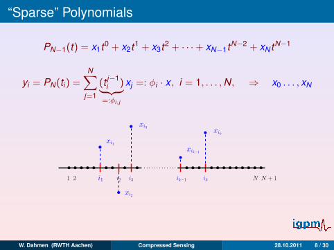
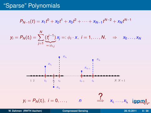
“Sparse” Polynomials
PN−1(t) = x1t0 + x2t1 + x3t2 + · · ·+ xN−1tN−2 + xN tN−1
yi = PN(ti) =N∑
j=1
(t j−1i )︸ ︷︷ ︸
=:φi,j
xj
=: φi · x
, i = 1, . . . ,N,
⇒ x0 . . . , xN
1
xi2
ikik−1i3i2i1
xik
xik−1
xi3
xi1
N + 12 N
yi = PN(ti), i = 0, . . . ,
? =
n
< N
?=⇒ xi1 . . . , xik
W. Dahmen (RWTH Aachen) Compressed Sensing 28.10.2011 8 / 30

“Sparse” Polynomials
PN−1(t) = x1t0 + x2t1 + x3t2 + · · ·+ xN−1tN−2 + xN tN−1
yi = PN(ti) =N∑
j=1
(t j−1i )︸ ︷︷ ︸
=:φi,j
xj =: φi · x , i = 1, . . . ,N,
⇒ x0 . . . , xN
1
xi2
ikik−1i3i2i1
xik
xik−1
xi3
xi1
N + 12 N
yi = PN(ti), i = 0, . . . ,
? =
n
< N
?=⇒ xi1 . . . , xik
W. Dahmen (RWTH Aachen) Compressed Sensing 28.10.2011 8 / 30

“Sparse” Polynomials
PN−1(t) = x1t0 + x2t1 + x3t2 + · · ·+ xN−1tN−2 + xN tN−1
yi = PN(ti) =N∑
j=1
(t j−1i )︸ ︷︷ ︸
=:φi,j
xj =: φi · x , i = 1, . . . ,N, ⇒ x0 . . . , xN
1
xi2
ikik−1i3i2i1
xik
xik−1
xi3
xi1
N + 12 N
yi = PN(ti), i = 0, . . . ,
? =
n
< N
?=⇒ xi1 . . . , xik
W. Dahmen (RWTH Aachen) Compressed Sensing 28.10.2011 8 / 30

“Sparse” Polynomials
PN−1(t) = x1t0 + x2t1 + x3t2 + · · ·+ xN−1tN−2 + xN tN−1
yi = PN(ti) =N∑
j=1
(t j−1i )︸ ︷︷ ︸
=:φi,j
xj =: φi · x , i = 1, . . . ,N, ⇒ x0 . . . , xN
1
xi2
ikik−1i3i2i1
xik
xik−1
xi3
xi1
N + 12 N
yi = PN(ti), i = 0, . . . ,? = n < N ?=⇒ xi1 . . . , xik
W. Dahmen (RWTH Aachen) Compressed Sensing 28.10.2011 8 / 30

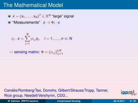
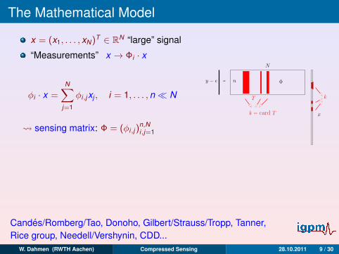
The Mathematical Model
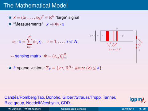
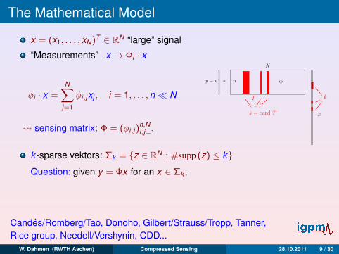
x = (x1, . . . , xN)T ∈ RN “large” signal
“Measurements” x → Φi · x
φi · x =N∑
j=1
φi,jxj , i = 1, . . . ,n N
sensing matrix: Φ = (φi,j )n,Ni,j=1
=
k
x
Φ
N
ny − e
k = card T
T
k -sparse vektors: Σk = z ∈ RN : #supp (z) ≤ kQuestion: given y = Φx for an x ∈ Σk ,
does there exist a decoder
∆ : Rn → RN , such that x = ∆(y),
for n ∼ k N
?
Candes/Romberg/Tao, Donoho, Gilbert/Strauss/Tropp, Tanner,Rice group, Needell/Vershynin, CDD...
W. Dahmen (RWTH Aachen) Compressed Sensing 28.10.2011 9 / 30
The Mathematical Model
x = (x1, . . . , xN)T ∈ RN “large” signal
“Measurements” x → Φi · x
φi · x =N∑
j=1
φi,jxj , i = 1, . . . ,n N
sensing matrix: Φ = (φi,j )n,Ni,j=1
=
k
x
Φ
N
ny − e
k = card T
T
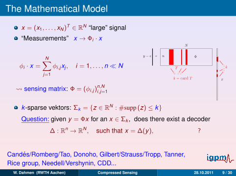
k -sparse vektors: Σk = z ∈ RN : #supp (z) ≤ k
Question: given y = Φx for an x ∈ Σk ,
does there exist a decoder
∆ : Rn → RN , such that x = ∆(y),
for n ∼ k N
?
Candes/Romberg/Tao, Donoho, Gilbert/Strauss/Tropp, Tanner,Rice group, Needell/Vershynin, CDD...
W. Dahmen (RWTH Aachen) Compressed Sensing 28.10.2011 9 / 30
The Mathematical Model
x = (x1, . . . , xN)T ∈ RN “large” signal
“Measurements” x → Φi · x
φi · x =N∑
j=1
φi,jxj , i = 1, . . . ,n N
sensing matrix: Φ = (φi,j )n,Ni,j=1
=
k
x
Φ
N
ny − e
k = card T
T
k -sparse vektors: Σk = z ∈ RN : #supp (z) ≤ kQuestion: given y = Φx for an x ∈ Σk ,
does there exist a decoder
∆ : Rn → RN , such that x = ∆(y),
for n ∼ k N
?
Candes/Romberg/Tao, Donoho, Gilbert/Strauss/Tropp, Tanner,Rice group, Needell/Vershynin, CDD...
W. Dahmen (RWTH Aachen) Compressed Sensing 28.10.2011 9 / 30
The Mathematical Model
x = (x1, . . . , xN)T ∈ RN “large” signal
“Measurements” x → Φi · x
φi · x =N∑
j=1
φi,jxj , i = 1, . . . ,n N
sensing matrix: Φ = (φi,j )n,Ni,j=1
=
k
x
Φ
N
ny − e
k = card T
T
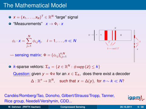
k -sparse vektors: Σk = z ∈ RN : #supp (z) ≤ kQuestion: given y = Φx for an x ∈ Σk , does there exist a decoder
∆ : Rn → RN , such that x = ∆(y),
for n ∼ k N
?
Candes/Romberg/Tao, Donoho, Gilbert/Strauss/Tropp, Tanner,Rice group, Needell/Vershynin, CDD...
W. Dahmen (RWTH Aachen) Compressed Sensing 28.10.2011 9 / 30
The Mathematical Model
x = (x1, . . . , xN)T ∈ RN “large” signal
“Measurements” x → Φi · x
φi · x =N∑
j=1
φi,jxj , i = 1, . . . ,n N
sensing matrix: Φ = (φi,j )n,Ni,j=1
=
k
x
Φ
N
ny − e
k = card T
T
k -sparse vektors: Σk = z ∈ RN : #supp (z) ≤ kQuestion: given y = Φx for an x ∈ Σk , does there exist a decoder
∆ : Rn → RN , such that x = ∆(y), for n ∼ k N?
Candes/Romberg/Tao, Donoho, Gilbert/Strauss/Tropp, Tanner,Rice group, Needell/Vershynin, CDD...
W. Dahmen (RWTH Aachen) Compressed Sensing 28.10.2011 9 / 30
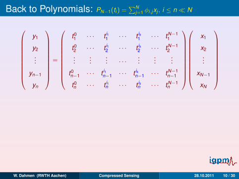
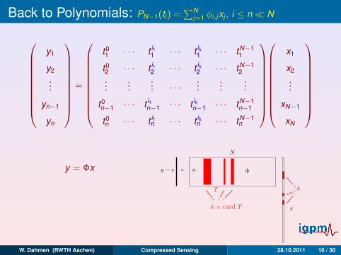
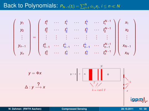
Back to Polynomials: PN−1(ti ) =∑N
j=1 φi,jxj , i ≤ n N
y1
y2
...
yn−1
yn
=
t01 · · · t i1
1 · · · t ik1 · · · tN−1
1
t02 · · · t i1
2 · · · t ik2 · · · tN−1
2...
...... · · ·
......
...
t0n−1 · · · t i1
n−1 · · · t ikn−1 · · · tN−1
n−1
t0n · · · t i1
n · · · t ikn · · · tN−1
n
x1
x2
...
xN−1
xN
y = Φx
∆ : y ?−→ x
=
k
x
Φ
N
ny − e
k = card T
T
W. Dahmen (RWTH Aachen) Compressed Sensing 28.10.2011 10 / 30

Are n ≥ 2k Measurements Sufficient?...
Σk := z ∈ RN : #supp (z) ≤ k,
ker Φ := z ∈ RN : Φz = 0
LEMMA:Let Φ ∈ Rn×N and 2k ≤ n. Then the following are equivalent:
(i) ∃ ∆ so that ∆(Φx) = x , for all x ∈ Σk ,
(ii) Σ2k ∩ ker Φ = 0,(iii) For any set of columns T with #T = 2k , the matrix ΦT has rank
2k .
Proof of: (i)⇒(ii): Suppose x ∈ Σ2k ∩ ker Φ x = x0 − x1 wherex0, x1 ∈ Σk . Since Φx0 = Φx1, (i) =⇒ x0 = x1 =⇒ x = x0 − x1 = 0.
W. Dahmen (RWTH Aachen) Compressed Sensing 28.10.2011 11 / 30

Are n ≥ 2k Measurements Sufficient?...
Σk := z ∈ RN : #supp (z) ≤ k,
ker Φ := z ∈ RN : Φz = 0
LEMMA:Let Φ ∈ Rn×N and 2k ≤ n. Then the following are equivalent:
(i) ∃ ∆ so that ∆(Φx) = x , for all x ∈ Σk ,(ii) Σ2k ∩ ker Φ = 0,
(iii) For any set of columns T with #T = 2k , the matrix ΦT has rank2k .
Proof of: (i)⇒(ii): Suppose x ∈ Σ2k ∩ ker Φ x = x0 − x1 wherex0, x1 ∈ Σk . Since Φx0 = Φx1, (i) =⇒ x0 = x1 =⇒ x = x0 − x1 = 0.
W. Dahmen (RWTH Aachen) Compressed Sensing 28.10.2011 11 / 30

Are n ≥ 2k Measurements Sufficient?...
Σk := z ∈ RN : #supp (z) ≤ k,
ker Φ := z ∈ RN : Φz = 0
LEMMA:Let Φ ∈ Rn×N and 2k ≤ n. Then the following are equivalent:
(i) ∃ ∆ so that ∆(Φx) = x , for all x ∈ Σk ,(ii) Σ2k ∩ ker Φ = 0,(iii) For any set of columns T with #T = 2k , the matrix ΦT has rank
2k .
Proof of: (i)⇒(ii): Suppose x ∈ Σ2k ∩ ker Φ x = x0 − x1 wherex0, x1 ∈ Σk . Since Φx0 = Φx1, (i) =⇒ x0 = x1 =⇒ x = x0 − x1 = 0.
W. Dahmen (RWTH Aachen) Compressed Sensing 28.10.2011 11 / 30

Are n ≥ 2k Measurements Sufficient?...
Σk := z ∈ RN : #supp (z) ≤ k,
ker Φ := z ∈ RN : Φz = 0
LEMMA:Let Φ ∈ Rn×N and 2k ≤ n. Then the following are equivalent:
(i) ∃ ∆ so that ∆(Φx) = x , for all x ∈ Σk ,(ii) Σ2k ∩ ker Φ = 0,(iii) For any set of columns T with #T = 2k , the matrix ΦT has rank
2k .
Proof of: (i)⇒(ii): Suppose x ∈ Σ2k ∩ ker Φ
x = x0 − x1 wherex0, x1 ∈ Σk . Since Φx0 = Φx1, (i) =⇒ x0 = x1 =⇒ x = x0 − x1 = 0.
W. Dahmen (RWTH Aachen) Compressed Sensing 28.10.2011 11 / 30

Are n ≥ 2k Measurements Sufficient?...
Σk := z ∈ RN : #supp (z) ≤ k,
ker Φ := z ∈ RN : Φz = 0
LEMMA:Let Φ ∈ Rn×N and 2k ≤ n. Then the following are equivalent:
(i) ∃ ∆ so that ∆(Φx) = x , for all x ∈ Σk ,(ii) Σ2k ∩ ker Φ = 0,(iii) For any set of columns T with #T = 2k , the matrix ΦT has rank
2k .
Proof of: (i)⇒(ii): Suppose x ∈ Σ2k ∩ ker Φ x = x0 − x1 wherex0, x1 ∈ Σk .
Since Φx0 = Φx1, (i) =⇒ x0 = x1 =⇒ x = x0 − x1 = 0.
W. Dahmen (RWTH Aachen) Compressed Sensing 28.10.2011 11 / 30

Are n ≥ 2k Measurements Sufficient?...
Σk := z ∈ RN : #supp (z) ≤ k,
ker Φ := z ∈ RN : Φz = 0
LEMMA:Let Φ ∈ Rn×N and 2k ≤ n. Then the following are equivalent:
(i) ∃ ∆ so that ∆(Φx) = x , for all x ∈ Σk ,(ii) Σ2k ∩ ker Φ = 0,(iii) For any set of columns T with #T = 2k , the matrix ΦT has rank
2k .
Proof of: (i)⇒(ii): Suppose x ∈ Σ2k ∩ ker Φ x = x0 − x1 wherex0, x1 ∈ Σk . Since Φx0 = Φx1, (i) =⇒ x0 = x1
=⇒ x = x0 − x1 = 0.
W. Dahmen (RWTH Aachen) Compressed Sensing 28.10.2011 11 / 30

Are n ≥ 2k Measurements Sufficient?...
Σk := z ∈ RN : #supp (z) ≤ k,
ker Φ := z ∈ RN : Φz = 0
LEMMA:Let Φ ∈ Rn×N and 2k ≤ n. Then the following are equivalent:
(i) ∃ ∆ so that ∆(Φx) = x , for all x ∈ Σk ,(ii) Σ2k ∩ ker Φ = 0,(iii) For any set of columns T with #T = 2k , the matrix ΦT has rank
2k .
Proof of: (i)⇒(ii): Suppose x ∈ Σ2k ∩ ker Φ x = x0 − x1 wherex0, x1 ∈ Σk . Since Φx0 = Φx1, (i) =⇒ x0 = x1 =⇒ x = x0 − x1 = 0.
W. Dahmen (RWTH Aachen) Compressed Sensing 28.10.2011 11 / 30

Polynomials Form a Descarte System
Are n = 2k measurements sufficient for k -sparse polynomials?
y1
y2...
yn−1
y2k
=
t01 · · · t i1
1 · · · t ik1 · · · tN−1
1
t02 · · · t i1
2 · · · t ik2 · · · tN−1
2...
...... · · · ...
......
t02k−1 · · · t i1
2k−1 · · · t ik2k−1 · · · tN−1
2k−1
t02k · · · t i1
2k · · · t ik2k · · · tN−1
2k
x1
x2...
xN−1
xN
...yes, all submatrices with 2k columns have full rank
BUT...
W. Dahmen (RWTH Aachen) Compressed Sensing 28.10.2011 12 / 30

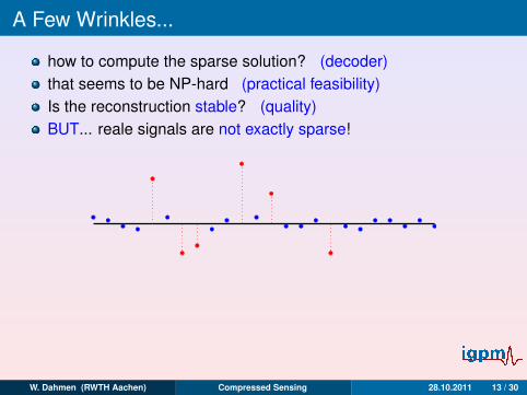
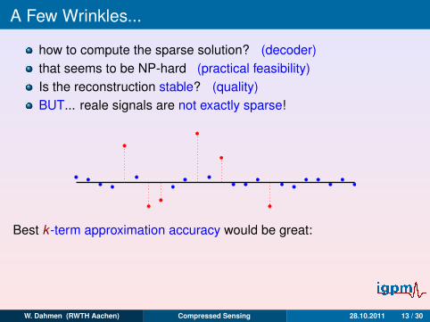
A Few Wrinkles...
how to compute the sparse solution? (decoder)
that seems to be NP-hard (practical feasibility)Is the reconstruction stable? (quality)BUT... reale signals are not exactly sparse!
Best k -term approximation accuracy would be great:
σk (x)`p := infz∈Σk‖x − z‖`p , ‖x‖`p :=
N∑j=1
|xj |p1/p
W. Dahmen (RWTH Aachen) Compressed Sensing 28.10.2011 13 / 30

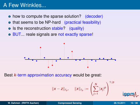
A Few Wrinkles...
how to compute the sparse solution? (decoder)that seems to be NP-hard (practical feasibility)
Is the reconstruction stable? (quality)BUT... reale signals are not exactly sparse!
Best k -term approximation accuracy would be great:
σk (x)`p := infz∈Σk‖x − z‖`p , ‖x‖`p :=
N∑j=1
|xj |p1/p
W. Dahmen (RWTH Aachen) Compressed Sensing 28.10.2011 13 / 30

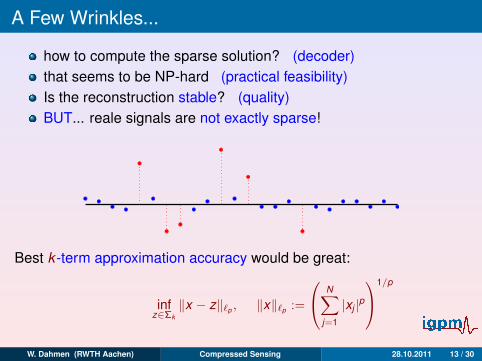
A Few Wrinkles...
how to compute the sparse solution? (decoder)that seems to be NP-hard (practical feasibility)Is the reconstruction stable? (quality)
BUT... reale signals are not exactly sparse!
Best k -term approximation accuracy would be great:
σk (x)`p := infz∈Σk‖x − z‖`p , ‖x‖`p :=
N∑j=1
|xj |p1/p
W. Dahmen (RWTH Aachen) Compressed Sensing 28.10.2011 13 / 30

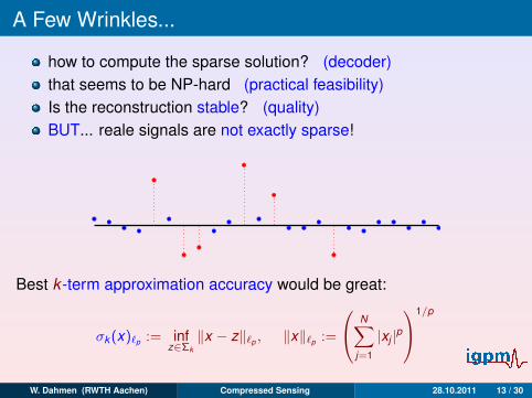
A Few Wrinkles...
how to compute the sparse solution? (decoder)that seems to be NP-hard (practical feasibility)Is the reconstruction stable? (quality)BUT... reale signals are not exactly sparse!
Best k -term approximation accuracy would be great:
σk (x)`p := infz∈Σk‖x − z‖`p , ‖x‖`p :=
N∑j=1
|xj |p1/p
W. Dahmen (RWTH Aachen) Compressed Sensing 28.10.2011 13 / 30
A Few Wrinkles...
how to compute the sparse solution? (decoder)that seems to be NP-hard (practical feasibility)Is the reconstruction stable? (quality)BUT... reale signals are not exactly sparse!
Best k -term approximation accuracy would be great:
σk (x)`p := infz∈Σk
‖x − z‖`p , ‖x‖`p :=
N∑j=1
|xj |p1/p
W. Dahmen (RWTH Aachen) Compressed Sensing 28.10.2011 13 / 30
A Few Wrinkles...
how to compute the sparse solution? (decoder)that seems to be NP-hard (practical feasibility)Is the reconstruction stable? (quality)BUT... reale signals are not exactly sparse!
Best k -term approximation accuracy would be great:
σk (x)`p :=
infz∈Σk‖x − z‖`p , ‖x‖`p :=
N∑j=1
|xj |p1/p
W. Dahmen (RWTH Aachen) Compressed Sensing 28.10.2011 13 / 30
A Few Wrinkles...
how to compute the sparse solution? (decoder)that seems to be NP-hard (practical feasibility)Is the reconstruction stable? (quality)BUT... reale signals are not exactly sparse!
Best k -term approximation accuracy would be great:
σk (x)`p := infz∈Σk‖x − z‖`p , ‖x‖`p :=
N∑j=1
|xj |p1/p
W. Dahmen (RWTH Aachen) Compressed Sensing 28.10.2011 13 / 30

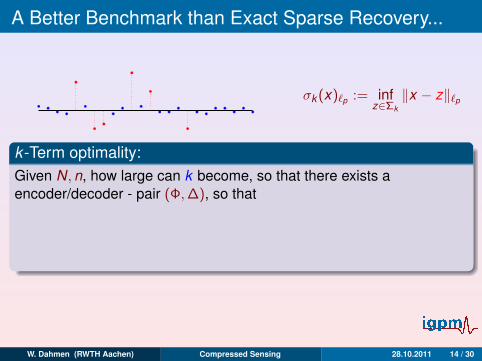
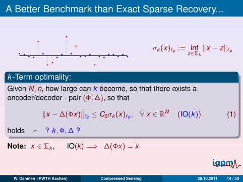
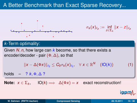
A Better Benchmark than Exact Sparse Recovery...
σk (x)`p := infz∈Σk
‖x − z‖`p
k -Term optimality:Given N,n, how large can k become, so that there exists aencoder/decoder - pair (Φ,∆), so that
‖x −∆(Φx)‖`2 ≤ C0σk (x)`2 , ∀ x ∈ RN
(IO(k)) (1)
holds
– ? k ,Φ,∆ ?
Note: x ∈ Σk , IO(k ) =⇒ ∆(Φx) = x exact reconstruction!
W. Dahmen (RWTH Aachen) Compressed Sensing 28.10.2011 14 / 30
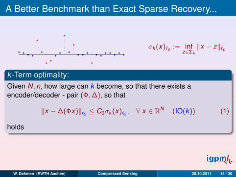
A Better Benchmark than Exact Sparse Recovery...
σk (x)`p := infz∈Σk
‖x − z‖`p
k -Term optimality:Given N,n, how large can k become, so that there exists aencoder/decoder - pair (Φ,∆), so that
‖x −∆(Φx)‖`2 ≤ C0σk (x)`2 , ∀ x ∈ RN (IO(k)) (1)
holds
– ? k ,Φ,∆ ?
Note: x ∈ Σk , IO(k ) =⇒ ∆(Φx) = x exact reconstruction!
W. Dahmen (RWTH Aachen) Compressed Sensing 28.10.2011 14 / 30
A Better Benchmark than Exact Sparse Recovery...
σk (x)`p := infz∈Σk
‖x − z‖`p
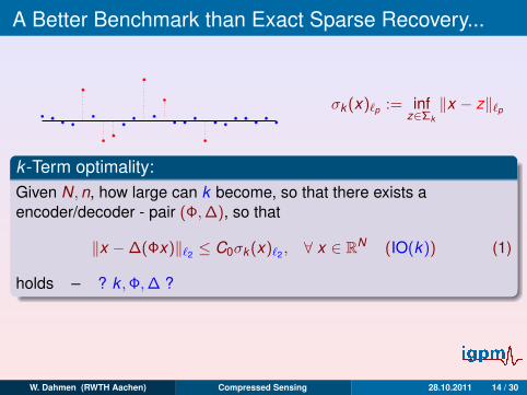
k -Term optimality:Given N,n, how large can k become, so that there exists aencoder/decoder - pair (Φ,∆), so that
‖x −∆(Φx)‖`2 ≤ C0σk (x)`2 , ∀ x ∈ RN (IO(k)) (1)
holds – ? k ,Φ,∆ ?
Note: x ∈ Σk , IO(k ) =⇒ ∆(Φx) = x exact reconstruction!
W. Dahmen (RWTH Aachen) Compressed Sensing 28.10.2011 14 / 30
A Better Benchmark than Exact Sparse Recovery...
σk (x)`p := infz∈Σk
‖x − z‖`p
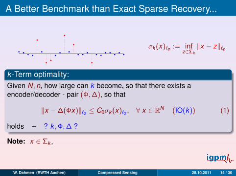
k -Term optimality:Given N,n, how large can k become, so that there exists aencoder/decoder - pair (Φ,∆), so that
‖x −∆(Φx)‖`2 ≤ C0σk (x)`2 , ∀ x ∈ RN (IO(k)) (1)
holds – ? k ,Φ,∆ ?
Note: x ∈ Σk ,
IO(k ) =⇒ ∆(Φx) = x exact reconstruction!
W. Dahmen (RWTH Aachen) Compressed Sensing 28.10.2011 14 / 30
A Better Benchmark than Exact Sparse Recovery...
σk (x)`p := infz∈Σk
‖x − z‖`p
k -Term optimality:Given N,n, how large can k become, so that there exists aencoder/decoder - pair (Φ,∆), so that
‖x −∆(Φx)‖`2 ≤ C0σk (x)`2 , ∀ x ∈ RN (IO(k)) (1)
holds – ? k ,Φ,∆ ?
Note: x ∈ Σk , IO(k ) =⇒ ∆(Φx) = x
exact reconstruction!
W. Dahmen (RWTH Aachen) Compressed Sensing 28.10.2011 14 / 30
A Better Benchmark than Exact Sparse Recovery...
σk (x)`p := infz∈Σk
‖x − z‖`p
k -Term optimality:Given N,n, how large can k become, so that there exists aencoder/decoder - pair (Φ,∆), so that
‖x −∆(Φx)‖`2 ≤ C0σk (x)`2 , ∀ x ∈ RN (IO(k)) (1)
holds – ? k ,Φ,∆ ?
Note: x ∈ Σk , IO(k ) =⇒ ∆(Φx) = x exact reconstruction!
W. Dahmen (RWTH Aachen) Compressed Sensing 28.10.2011 14 / 30

Guiding Questions
What is the maximal optimality range k?
Which sensing matrices Φ achieve the maximal range?
How to develop k -term optimal decoders?
W. Dahmen (RWTH Aachen) Compressed Sensing 28.10.2011 15 / 30

Guiding Questions
What is the maximal optimality range k?
Which sensing matrices Φ achieve the maximal range?
How to develop k -term optimal decoders?
W. Dahmen (RWTH Aachen) Compressed Sensing 28.10.2011 15 / 30

Guiding Questions
What is the maximal optimality range k?
Which sensing matrices Φ achieve the maximal range?
How to develop k -term optimal decoders?
W. Dahmen (RWTH Aachen) Compressed Sensing 28.10.2011 15 / 30

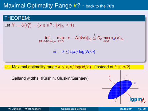
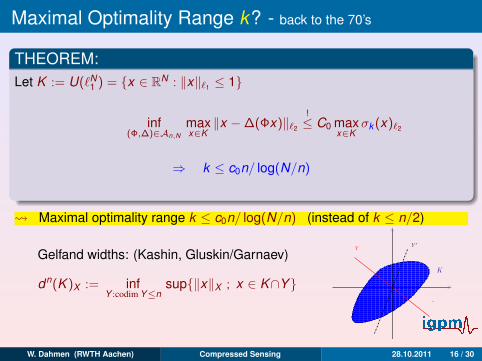
Maximal Optimality Range k? - back to the 70’s
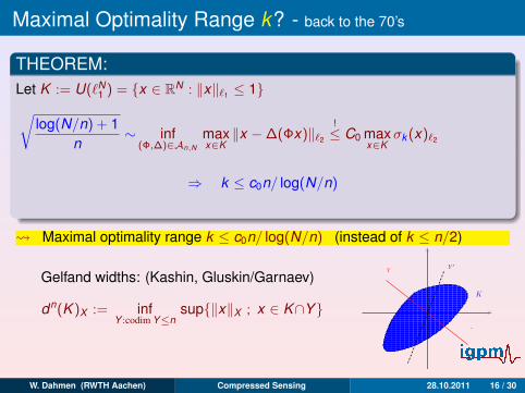
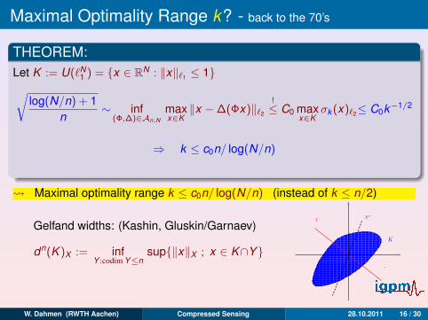
THEOREM:
Let K := U(`N1 ) = x ∈ RN : ‖x‖`1 ≤ 1√
log(N/n) + 1n
∼ inf(Φ,∆)∈An,N
maxx∈K
‖x −∆(Φx)‖`2
!≤ C0
maxx∈K
σk (x)`2
≤ C0k−1/2
⇒ k ≤ c0n/ log(N/n)
Maximal optimality range k ≤ c0n/ log(N/n) (instead of k ≤ n/2)
Gelfand widths: (Kashin, Gluskin/Garnaev)
dn(K )X := infY :codim Y≤n
sup‖x‖X ; x ∈ K∩Y
K
Y ′Y
W. Dahmen (RWTH Aachen) Compressed Sensing 28.10.2011 16 / 30

Maximal Optimality Range k? - back to the 70’s
THEOREM:Let K := U(`N
1 ) = x ∈ RN : ‖x‖`1 ≤ 1
√log(N/n) + 1
n∼ inf
(Φ,∆)∈An,N
maxx∈K‖x −∆(Φx)‖`2
!≤ C0 max
x∈Kσk (x)`2
≤ C0k−1/2
⇒ k ≤ c0n/ log(N/n)
Maximal optimality range k ≤ c0n/ log(N/n) (instead of k ≤ n/2)
Gelfand widths: (Kashin, Gluskin/Garnaev)
dn(K )X := infY :codim Y≤n
sup‖x‖X ; x ∈ K∩Y
K
Y ′Y
W. Dahmen (RWTH Aachen) Compressed Sensing 28.10.2011 16 / 30

Maximal Optimality Range k? - back to the 70’s
THEOREM:Let K := U(`N
1 ) = x ∈ RN : ‖x‖`1 ≤ 1
√log(N/n) + 1
n∼
inf(Φ,∆)∈An,N
maxx∈K‖x −∆(Φx)‖`2
!≤ C0 max
x∈Kσk (x)`2
≤ C0k−1/2
⇒ k ≤ c0n/ log(N/n)
Maximal optimality range k ≤ c0n/ log(N/n) (instead of k ≤ n/2)
Gelfand widths: (Kashin, Gluskin/Garnaev)
dn(K )X := infY :codim Y≤n
sup‖x‖X ; x ∈ K∩Y
K
Y ′Y
W. Dahmen (RWTH Aachen) Compressed Sensing 28.10.2011 16 / 30
Maximal Optimality Range k? - back to the 70’s
THEOREM:Let K := U(`N
1 ) = x ∈ RN : ‖x‖`1 ≤ 1√log(N/n) + 1
n∼ inf
(Φ,∆)∈An,N
maxx∈K‖x −∆(Φx)‖`2
!≤ C0 max
x∈Kσk (x)`2
≤ C0k−1/2
⇒ k ≤ c0n/ log(N/n)
Maximal optimality range k ≤ c0n/ log(N/n) (instead of k ≤ n/2)
Gelfand widths: (Kashin, Gluskin/Garnaev)
dn(K )X := infY :codim Y≤n
sup‖x‖X ; x ∈ K∩Y
K
Y ′Y
W. Dahmen (RWTH Aachen) Compressed Sensing 28.10.2011 16 / 30
Maximal Optimality Range k? - back to the 70’s
THEOREM:Let K := U(`N
1 ) = x ∈ RN : ‖x‖`1 ≤ 1√log(N/n) + 1
n∼ inf
(Φ,∆)∈An,N
maxx∈K‖x −∆(Φx)‖`2
!≤ C0 max
x∈Kσk (x)`2≤ C0k−1/2
⇒ k ≤ c0n/ log(N/n)
Maximal optimality range k ≤ c0n/ log(N/n) (instead of k ≤ n/2)
Gelfand widths: (Kashin, Gluskin/Garnaev)
dn(K )X := infY :codim Y≤n
sup‖x‖X ; x ∈ K∩Y
K
Y ′Y
W. Dahmen (RWTH Aachen) Compressed Sensing 28.10.2011 16 / 30

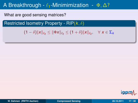
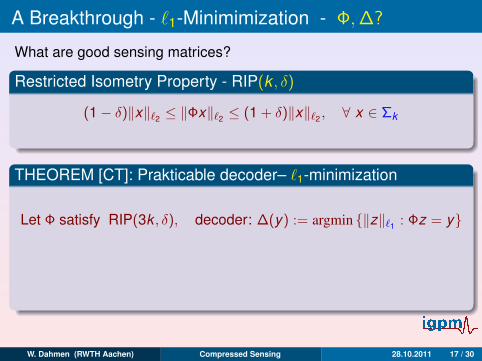
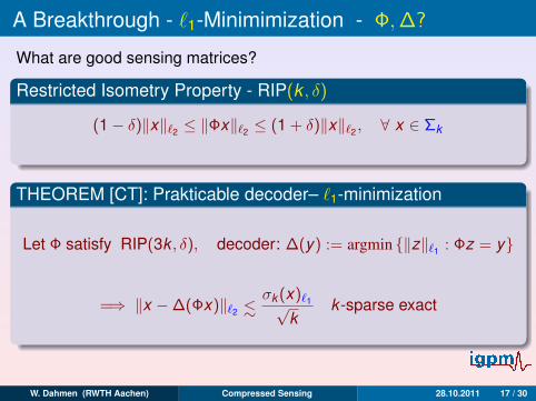
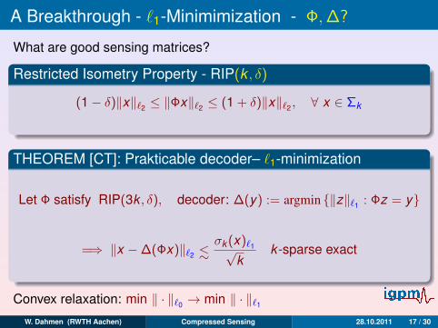
A Breakthrough - `1-Minimimization - Φ,∆?
What are good sensing matrices?
Restricted Isometry Property - RIP(k , δ)
(1− δ)‖x‖`2 ≤ ‖Φx‖`2 ≤ (1 + δ)‖x‖`2 , ∀ x ∈ Σk
THEOREM [CT]: Prakticable decoder– `1-minimization
Let Φ satisfy RIP(3k , δ), decoder: ∆(y) := argmin ‖z‖`1 : Φz = y
=⇒ ‖x −∆(Φx)‖`2 <∼σk (x)`1√
kk -sparse exact
Convex relaxation: min ‖ · ‖`0 → min ‖ · ‖`1
W. Dahmen (RWTH Aachen) Compressed Sensing 28.10.2011 17 / 30
A Breakthrough - `1-Minimimization - Φ,∆?
What are good sensing matrices?
Restricted Isometry Property - RIP(k , δ)
(1− δ)‖x‖`2 ≤ ‖Φx‖`2 ≤ (1 + δ)‖x‖`2 , ∀ x ∈ Σk
THEOREM [CT]: Prakticable decoder– `1-minimization
Let Φ satisfy RIP(3k , δ), decoder: ∆(y) := argmin ‖z‖`1 : Φz = y
=⇒ ‖x −∆(Φx)‖`2 <∼σk (x)`1√
kk -sparse exact
Convex relaxation: min ‖ · ‖`0 → min ‖ · ‖`1W. Dahmen (RWTH Aachen) Compressed Sensing 28.10.2011 17 / 30
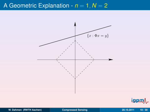
A Geometric Explanation - n = 1,N = 2
x : Φx = y
W. Dahmen (RWTH Aachen) Compressed Sensing 28.10.2011 18 / 30

A Geometric Explanation - n = 1,N = 2
x : Φx = y
W. Dahmen (RWTH Aachen) Compressed Sensing 28.10.2011 19 / 30

Closely Related: TV-Minimization... - ∆?
(Candes/Romberg/Tao)
W. Dahmen (RWTH Aachen) Compressed Sensing 28.10.2011 20 / 30
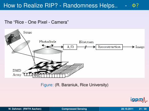
How to Realize RIP? - Randomness Helps.. - Φ?
The “Rice - One Pixel - Camera”
Figure: (R. Baraniuk, Rice University)
W. Dahmen (RWTH Aachen) Compressed Sensing 28.10.2011 21 / 30

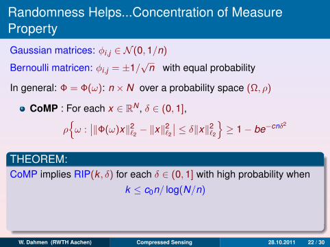
Randomness Helps...Concentration of MeasureProperty
Gaussian matrices: φi,j ∈ N (0,1/n)
Bernoulli matricen: φi,j = ±1/√
n with equal probability
In general: Φ = Φ(ω): n × N over a probability space (Ω, ρ)
CoMP : For each x ∈ RN , δ ∈ (0,1],
ρω :∣∣‖Φ(ω)x‖2`2 − ‖x‖
2`2
∣∣ ≤ δ‖x‖2`2 ≥ 1− be−cnδ2
THEOREM:CoMP implies RIP(k , δ) for each δ ∈ (0,1] with high probability when
k ≤ c0n/ log(N/n)
Gauß-, Bernoulli-, uniformly distributed points on the (n − 1)-spheresatisfy CoMP
W. Dahmen (RWTH Aachen) Compressed Sensing 28.10.2011 22 / 30

Randomness Helps...Concentration of MeasureProperty
Gaussian matrices: φi,j ∈ N (0,1/n)
Bernoulli matricen: φi,j = ±1/√
n with equal probability
In general: Φ = Φ(ω): n × N over a probability space (Ω, ρ)
CoMP : For each x ∈ RN , δ ∈ (0,1],
ρω :
∣∣‖Φ(ω)x‖2`2 − ‖x‖2`2
∣∣ ≤ δ‖x‖2`2
≥ 1− be−cnδ2
THEOREM:CoMP implies RIP(k , δ) for each δ ∈ (0,1] with high probability when
k ≤ c0n/ log(N/n)
Gauß-, Bernoulli-, uniformly distributed points on the (n − 1)-spheresatisfy CoMP
W. Dahmen (RWTH Aachen) Compressed Sensing 28.10.2011 22 / 30

Randomness Helps...Concentration of MeasureProperty
Gaussian matrices: φi,j ∈ N (0,1/n)
Bernoulli matricen: φi,j = ±1/√
n with equal probability
In general: Φ = Φ(ω): n × N over a probability space (Ω, ρ)
CoMP : For each x ∈ RN , δ ∈ (0,1],
ρω :∣∣‖Φ(ω)x‖2`2 − ‖x‖
2`2
∣∣ ≤ δ‖x‖2`2 ≥ 1− be−cnδ2
THEOREM:CoMP implies RIP(k , δ) for each δ ∈ (0,1] with high probability when
k ≤ c0n/ log(N/n)
Gauß-, Bernoulli-, uniformly distributed points on the (n − 1)-spheresatisfy CoMP
W. Dahmen (RWTH Aachen) Compressed Sensing 28.10.2011 22 / 30

Randomness Helps...Concentration of MeasureProperty
Gaussian matrices: φi,j ∈ N (0,1/n)
Bernoulli matricen: φi,j = ±1/√
n with equal probability
In general: Φ = Φ(ω): n × N over a probability space (Ω, ρ)
CoMP : For each x ∈ RN , δ ∈ (0,1],
ρω :∣∣‖Φ(ω)x‖2`2 − ‖x‖
2`2
∣∣ ≤ δ‖x‖2`2 ≥ 1− be−cnδ2
THEOREM:CoMP implies RIP(k , δ) for each δ ∈ (0,1] with high probability when
k ≤ c0n/ log(N/n)
Gauß-, Bernoulli-, uniformly distributed points on the (n − 1)-spheresatisfy CoMP
W. Dahmen (RWTH Aachen) Compressed Sensing 28.10.2011 22 / 30

The Norm Matters...
THEOREM: ‖x‖`1 =∑N
j=1 |xj |:Assume that Φ satisfies RIP(3k , δ) and ∆(y) := argminΦz=y‖z‖`1
=⇒‖x −∆(Φx)‖`1 ≤ C(δ)σk (x)`1
THEOREM: ‖x‖`2 =(∑N
j=1 |xj |2)1/2
:
• For each (Φ,∆) : 1-term optimality ∀ x ∈ RN =⇒ n ≥ aN
• Assume that Φ(ω) satisfies CoMP. Then ∃ ∆ s.t. for each x ∈ RN
with high probability (with respect to .Φ) one has
‖x −∆(Φx)‖`2 ≤ C0σk (x)`2 , k <∼ n/ log(N/n)
W. Dahmen (RWTH Aachen) Compressed Sensing 28.10.2011 23 / 30

The Norm Matters...
THEOREM: ‖x‖`1 =∑N
j=1 |xj |:Assume that Φ satisfies RIP(3k , δ) and ∆(y) := argminΦz=y‖z‖`1=⇒
‖x −∆(Φx)‖`1 ≤ C(δ)σk (x)`1
THEOREM: ‖x‖`2 =(∑N
j=1 |xj |2)1/2
:
• For each (Φ,∆) : 1-term optimality ∀ x ∈ RN =⇒ n ≥ aN
• Assume that Φ(ω) satisfies CoMP. Then ∃ ∆ s.t. for each x ∈ RN
with high probability (with respect to .Φ) one has
‖x −∆(Φx)‖`2 ≤ C0σk (x)`2 , k <∼ n/ log(N/n)
W. Dahmen (RWTH Aachen) Compressed Sensing 28.10.2011 23 / 30
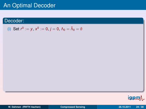
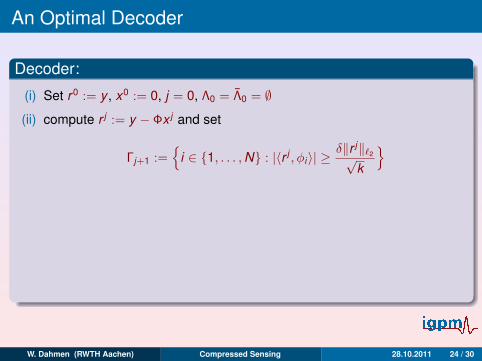
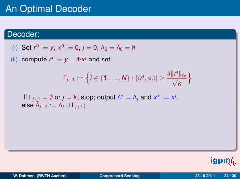
An Optimal Decoder
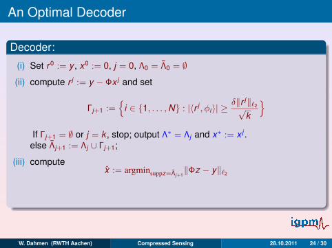
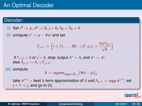
Decoder:
(i) Set r0 := y , x0 := 0, j = 0, Λ0 = Λ0 = ∅
(ii) compute r j := y − Φx j and set
Γj+1 :=
i ∈ 1, . . . ,N : |〈r j , φi〉| ≥δ‖r j‖`2√
k
If Γj+1 = ∅ or j = k , stop; output Λ∗ = Λj and x∗ := x j .else Λj+1 := Λj ∪ Γj+1;
(iii) computex := argminsuppz=Λj+1
‖Φz − y‖`2
take x j+1 = best k -term approximation of x und Λj+1 := supp x j+1, setj + 1→ j , and go to (ii).
W. Dahmen (RWTH Aachen) Compressed Sensing 28.10.2011 24 / 30
An Optimal Decoder
Decoder:
(i) Set r0 := y , x0 := 0, j = 0, Λ0 = Λ0 = ∅(ii) compute r j := y − Φx j and set
Γj+1 :=
i ∈ 1, . . . ,N : |〈r j , φi〉| ≥δ‖r j‖`2√
k
If Γj+1 = ∅ or j = k , stop; output Λ∗ = Λj and x∗ := x j .
else Λj+1 := Λj ∪ Γj+1;
(iii) computex := argminsuppz=Λj+1
‖Φz − y‖`2
take x j+1 = best k -term approximation of x und Λj+1 := supp x j+1, setj + 1→ j , and go to (ii).
W. Dahmen (RWTH Aachen) Compressed Sensing 28.10.2011 24 / 30

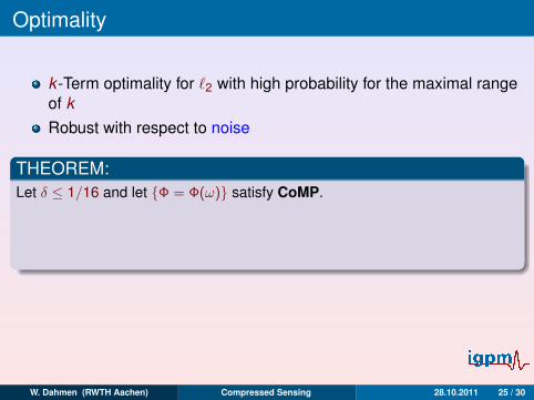
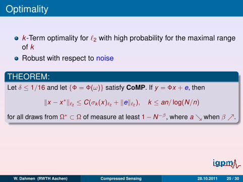
Optimality
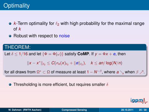
k -Term optimality for `2 with high probability for the maximal rangeof k
Robust with respect to noise
THEOREM:Let δ ≤ 1/16 and let Φ = Φ(ω) satisfy CoMP.
If y = Φx + e, then
‖x − x∗‖`2 ≤ C(σk (x)`2 + ‖e‖`2 ), k ≤ an/ log(N/n)
for all draws from Ω∗ ⊂ Ω of measure at least 1−N−β , where a when β .
Thresholding is more efficient, but requires smaller δ
`1-minimimization/regularization is more robust but more expensive...
W. Dahmen (RWTH Aachen) Compressed Sensing 28.10.2011 25 / 30

Optimality
k -Term optimality for `2 with high probability for the maximal rangeof kRobust with respect to noise
THEOREM:Let δ ≤ 1/16 and let Φ = Φ(ω) satisfy CoMP.
If y = Φx + e, then
‖x − x∗‖`2 ≤ C(σk (x)`2 + ‖e‖`2 ), k ≤ an/ log(N/n)
for all draws from Ω∗ ⊂ Ω of measure at least 1−N−β , where a when β .
Thresholding is more efficient, but requires smaller δ
`1-minimimization/regularization is more robust but more expensive...
W. Dahmen (RWTH Aachen) Compressed Sensing 28.10.2011 25 / 30
Optimality
k -Term optimality for `2 with high probability for the maximal rangeof kRobust with respect to noise
THEOREM:Let δ ≤ 1/16 and let Φ = Φ(ω) satisfy CoMP. If y = Φx + e, then
‖x − x∗‖`2 ≤ C(σk (x)`2 + ‖e‖`2 ), k ≤ an/ log(N/n)
for all draws from Ω∗ ⊂ Ω of measure at least 1−N−β , where a when β .
Thresholding is more efficient, but requires smaller δ
`1-minimimization/regularization is more robust but more expensive...
W. Dahmen (RWTH Aachen) Compressed Sensing 28.10.2011 25 / 30
Optimality
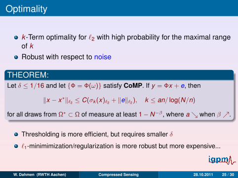
k -Term optimality for `2 with high probability for the maximal rangeof kRobust with respect to noise
THEOREM:Let δ ≤ 1/16 and let Φ = Φ(ω) satisfy CoMP. If y = Φx + e, then
‖x − x∗‖`2 ≤ C(σk (x)`2 + ‖e‖`2 ), k ≤ an/ log(N/n)
for all draws from Ω∗ ⊂ Ω of measure at least 1−N−β , where a when β .
Thresholding is more efficient, but requires smaller δ
`1-minimimization/regularization is more robust but more expensive...
W. Dahmen (RWTH Aachen) Compressed Sensing 28.10.2011 25 / 30

`1-Regularization
x
||e||ℓ2 ≤ ηΦ2
Φ1
n2
n1
y2
y1
=e
+
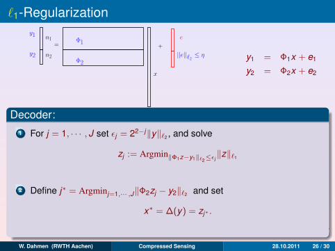
y1 = Φ1x + e1
y2 = Φ2x + e2
Decoder:1 For j = 1, · · · , J set εj = 22−j‖y‖`2 , and solve
zj := Argmin‖Φ1z−y1‖`2≤εj‖z‖`1
2 Define j∗ = Argminj=1,··· ,J‖Φ2zj − y2‖`2 and set
x∗ = ∆(y) = zj∗ .
W. Dahmen (RWTH Aachen) Compressed Sensing 28.10.2011 26 / 30

`1-Regularization
x
||e||ℓ2 ≤ ηΦ2
Φ1
n2
n1
y2
y1
=e
+
y1 = Φ1x + e1
y2 = Φ2x + e2
Decoder:1 For j = 1, · · · , J set εj = 22−j‖y‖`2 , and solve
zj := Argmin‖Φ1z−y1‖`2≤εj‖z‖`1
2 Define j∗ = Argminj=1,··· ,J‖Φ2zj − y2‖`2
and set
x∗ = ∆(y) = zj∗ .
W. Dahmen (RWTH Aachen) Compressed Sensing 28.10.2011 26 / 30
`1-Regularization
x
||e||ℓ2 ≤ ηΦ2
Φ1
n2
n1
y2
y1
=e
+
y1 = Φ1x + e1
y2 = Φ2x + e2
Decoder:1 For j = 1, · · · , J set εj = 22−j‖y‖`2 , and solve
zj := Argmin‖Φ1z−y1‖`2≤εj‖z‖`1
2 Define j∗ = Argminj=1,··· ,J‖Φ2zj − y2‖`2 and set
x∗ = ∆(y) = zj∗ .
W. Dahmen (RWTH Aachen) Compressed Sensing 28.10.2011 26 / 30

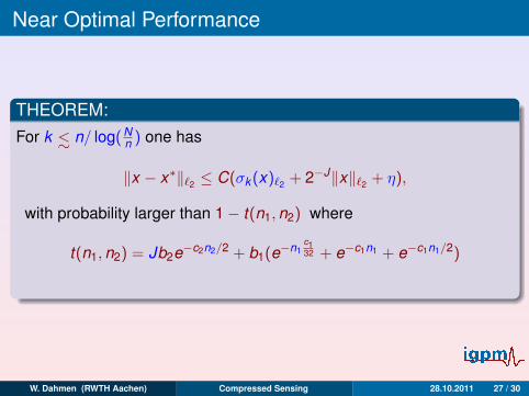
Near Optimal Performance
THEOREM:For k <∼ n/ log(N
n ) one has
‖x − x∗‖`2 ≤ C(σk (x)`2 + 2−J‖x‖`2 + η),
with probability larger than 1− t(n1,n2) where
t(n1,n2) = Jb2e−c2n2/2 + b1(e−n1c132 + e−c1n1 + e−c1n1/2)
W. Dahmen (RWTH Aachen) Compressed Sensing 28.10.2011 27 / 30

Near Optimal Performance
THEOREM:For k <∼ n/ log(N
n ) one has
‖x − x∗‖`2 ≤ C(σk (x)`2 + 2−J‖x‖`2 + η),
with probability larger than 1− t(n1,n2) where
t(n1,n2) = Jb2e−c2n2/2 + b1(e−n1c132 + e−c1n1 + e−c1n1/2)
W. Dahmen (RWTH Aachen) Compressed Sensing 28.10.2011 27 / 30
Near Optimal Performance
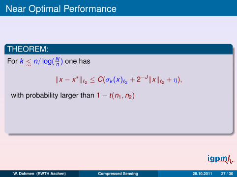
THEOREM:For k <∼ n/ log(N
n ) one has
‖x − x∗‖`2 ≤ C(σk (x)`2 + 2−J‖x‖`2 + η),
with probability larger than 1− t(n1,n2)
where
t(n1,n2) = Jb2e−c2n2/2 + b1(e−n1c132 + e−c1n1 + e−c1n1/2)
W. Dahmen (RWTH Aachen) Compressed Sensing 28.10.2011 27 / 30
Near Optimal Performance
THEOREM:For k <∼ n/ log(N
n ) one has
‖x − x∗‖`2 ≤ C(σk (x)`2 + 2−J‖x‖`2 + η),
with probability larger than 1− t(n1,n2) where
t(n1,n2) = Jb2e−c2n2/2 + b1(e−n1c132 + e−c1n1 + e−c1n1/2)
W. Dahmen (RWTH Aachen) Compressed Sensing 28.10.2011 27 / 30

Electron-Tomography
W. Dahmen (RWTH Aachen) Compressed Sensing 28.10.2011 28 / 30
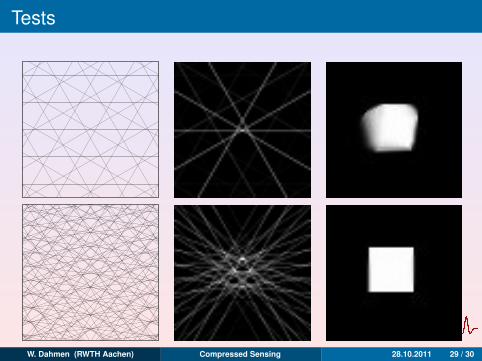
Tests
Figure: Reconstructions from noise free data with a maximum tilt angle of60o. First column: ray trace diagrams of the measurents taken. Secondcolumn: least-squares reconstruction computed with Kaczmarz iterations.Third column: TV-regularized reconstruction. First row: na = 5, H = 1/5.Second row: na = 10, H = 1/10. Third row: na = 20, H = 1/32. Fourth row:na = 20, H = 1/32.
W. Dahmen (RWTH Aachen) Compressed Sensing 28.10.2011 29 / 30
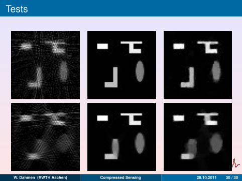
Tests
Figure: Reconstruction of a rotated Phantom 2. Same parameters as inFigure ??: na = 20, H = 1/32. Top row: Θmax = 85o, Bottom Row:Θmax = 60o. First and second column: Kaczmarz and TV-reconstruction fromnoise-free data . Third column: TV-reconstruction from noisy data (σ = 2,erel (d) = 0.077). µopt = 0.07 and 0.12 for Θmax = 85o and Θmax = 60o,respectively.
W. Dahmen (RWTH Aachen) Compressed Sensing 28.10.2011 30 / 30