ANOVA

Comparing the means of more

than two groups

Analysis of variance (ANOVA)

•! Like a t-test, but can compare more

than two groups

•! Asks whether any of two or more means

is different from any other.

•! In other words, is the variance among

groups greater than 0?

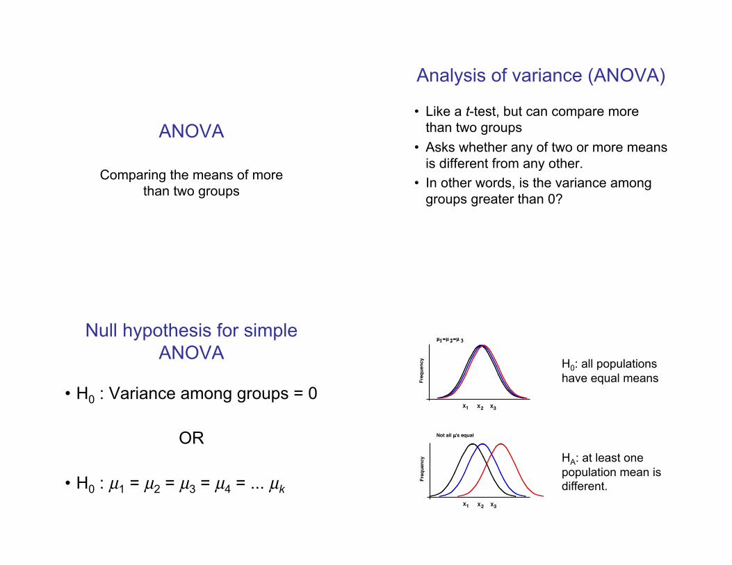
Null hypothesis for simple

ANOVA

•!H0 : Variance among groups = 0

OR

•!H0 : µ1 = µ2 = µ3 = µ4 = ... µk

X1 X2 X3

Fre

qu

en

cy

µ1 = µ 2 = µ 3

X1 X2 X3

Fre

qu

en

cy

Not all µ's equal

H0: all populations

have equal means

HA: at least one

population mean is

different.

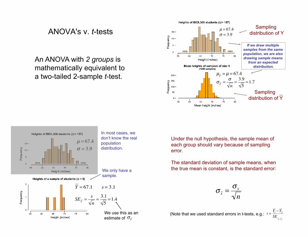
ANOVA's v. t-tests

An ANOVA with 2 groups is

mathematically equivalent to

a two-tailed 2-sample t-test.

µ = 67.4

! = 3.9

µY

= µ = 67.4

!Y

=!

n=3.9

5=1.7

N

Sampling

distribution of Y

Sampling

distribution of Y

If we draw multiple

samples from the same

population, we are also

drawing sample means

from an expected

distribution.

µ = 67.4

! = 3.9

N In most cases, we

don"t know the real

population distribution.#

We only have a

sample.#

SEY

=s

n=3.1

5=1.4

We use this as an

estimate of #

!Y

s = 3.1

Y = 67.1

!x

=!

x

n

Under the null hypothesis, the sample mean of

each group should vary because of sampling

error.

The standard deviation of sample means, when

the true mean is constant, is the standard error:

t =Y 1!Y

2

SEY 1!Y 2

(Note that we used standard errors in t-tests, e.g.:

!x

2=!

x

2

n

Squaring the standard error, the variance

among groups due to sampling error should be:

In ANOVA, we work with variances rather than

standard deviations.

!x

2 =!

x

2

n+ Variance µ

i[ ]

If the null hypothesis is not true, the

variance among groups should be

equal to the variance due to

sampling error plus the real variance

among population means.

With ANOVA, we test whether the

variance among true group means is

greater than zero.

We do this by asking whether the

observed variance among groups is

greater than expected by chance

(assuming the null is true):

!x

2>!

x

2

n?

!x

2>!

x

2

n?

n!x

2> !

x

2?

n!x

2 is estimated by the

“Mean Squares Group”

!x

2 is the variance within groups,

estimated by the

“Mean Squares Error”

MSgroup

MSerror

Population parameters Estimates from sample

n !x

2 + Variance µi[ ]( )

MSgroup

Mean squares group

Abbreviation:

Estimates this parameter:

Formula:

MSgroups =SSgroups

dfgroups

Mean squares group

SSgroup = ni X i ! X ( )2

"

dfgroup = k-1

MSgroups =SSgroups

dfgroups

Mean squares error

Abbreviation:

Estimates this parameter:

Formula:

MSerror =SSerror

dferror

!x

2

MSerror

Mean squares error Error sum of squares =

SSerror = dfisi2

= si2(ni !1)""

Error degrees of freedom =

dferror = dfi = ni !1( )"" = N ! k

MSerror is like the pooled variance in a 2-sample t-test:

MSerror =SSerror

dferror=

si2(ni !1)"

N ! k

sp2

=df1s1

2+ df

2s2

2

df1

+ df2

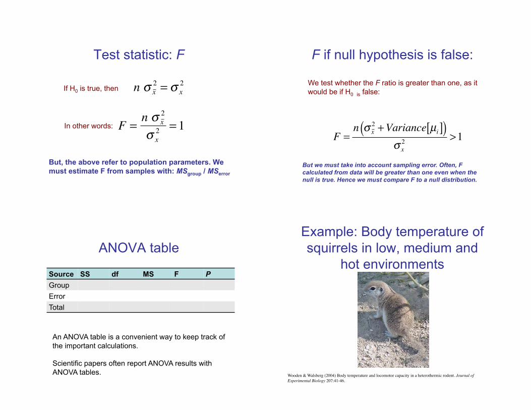
Test statistic: F

If H0 is true, then

n !x

2= !

x

2

In other words:

F =n !

x

2

!x

2= 1

But, the above refer to population parameters. We

must estimate F from samples with: MSgroup / MSerror

F if null hypothesis is false:

We test whether the F ratio is greater than one, as it

would be if H0 is false:

F =n !

x

2 + Variance µi[ ]( )

!x

2>1

But we must take into account sampling error. Often, F

calculated from data will be greater than one even when the

null is true. Hence we must compare F to a null distribution.

ANOVA table

Source SS df MS F P

Group

Error

Total

An ANOVA table is a convenient way to keep track of

the important calculations.

Scientific papers often report ANOVA results with

ANOVA tables.

Example: Body temperature of

squirrels in low, medium and

hot environments

Wooden & Walsberg (2004) Body temperature and locomotor capacity in a heterothermic rodent. Journal of

Experimental Biology 207:41-46.!

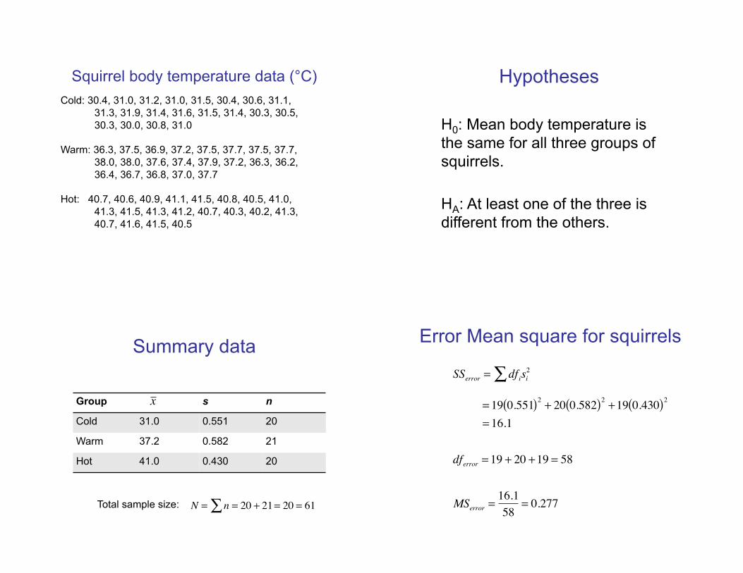
Squirrel body temperature data (°C)

Cold: 30.4, 31.0, 31.2, 31.0, 31.5, 30.4, 30.6, 31.1,

31.3, 31.9, 31.4, 31.6, 31.5, 31.4, 30.3, 30.5,

30.3, 30.0, 30.8, 31.0

Warm: 36.3, 37.5, 36.9, 37.2, 37.5, 37.7, 37.5, 37.7,

38.0, 38.0, 37.6, 37.4, 37.9, 37.2, 36.3, 36.2,

36.4, 36.7, 36.8, 37.0, 37.7

Hot: 40.7, 40.6, 40.9, 41.1, 41.5, 40.8, 40.5, 41.0,

41.3, 41.5, 41.3, 41.2, 40.7, 40.3, 40.2, 41.3,

40.7, 41.6, 41.5, 40.5

Hypotheses

H0: Mean body temperature is

the same for all three groups of

squirrels.

HA: At least one of the three is

different from the others.

Summary data

Group s n

Cold 31.0 0.551 20

Warm 37.2 0.582 21

Hot 41.0 0.430 20

x

Total sample size:

N = n! = 20 + 21= 20 = 61

Error Mean square for squirrels

SSerror = dfisi2!

= 19 0.551( )2

+ 20 0.582( )2

+19 0.430( )2

= 16.1

dferror = 19 + 20 +19 = 58

MSerror =16.1

58= 0.277

Squirrel Mean Squares Group:

X =20 31.0( ) + 21 37.2( ) + 20 41.0( )

20 + 21+ 20= 36.4

SSgroup = 20(31.0-36.4)2 +21(37.2-36.4)2 +20(41.0-36.4)2!

=1015.7!

SSgroup = ni X i ! X ( )2

"

Squirrel Mean Squares Group:

dfgroup= k – 1 = 3-1=2

MSgroups =SSgroups

dfgroups=1015.7

2= 507.9

The test statistic for ANOVA is

F

F =MSgroup

MSerror=507.9

0.277= 1834.7

MSgroupis always in the numerator,

MSerror is always in the denominator

Compare to F!(1),df_group,df_error

F0.05(1),2,58 = 3.15.

Since 1835 > 3.15, we know P < 0.05 and we can

reject the null hypothesis.

The variance in sample group means is bigger than

expected given the variance within sample groups.

Therefore, at least one of the groups has a population

mean different from another group.

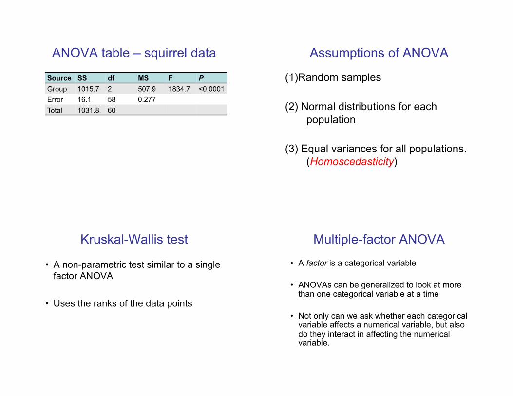
ANOVA table – squirrel data

Source SS df MS F P

Group 1015.7 2 507.9 1834.7 <0.0001

Error 16.1 58 0.277

Total 1031.8 60

Assumptions of ANOVA

(1)!Random samples

(2)! Normal distributions for each

population

(3) Equal variances for all populations.

(Homoscedasticity)

Kruskal-Wallis test

•! A non-parametric test similar to a single

factor ANOVA

•! Uses the ranks of the data points

Multiple-factor ANOVA

•! A factor is a categorical variable

•! ANOVAs can be generalized to look at more than one categorical variable at a time

•! Not only can we ask whether each categorical variable affects a numerical variable, but also do they interact in affecting the numerical variable.

Fixed vs. random effects

1.! Fixed effects: With fixed effects, the treatments are

chosen by the experimenter. They are not a

random subset of all possible treatments. (e.g., specific drug treatments, specific diets,

season...)

2. Random effects: With random effects, the

treatments are a random sample from all possible treatments.

(e.g., family, location, ...)

For single-factor ANOVAs, there is no difference in the statistics for fixed or random effects.

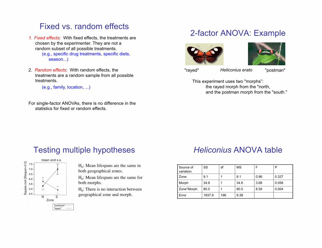
2-factor ANOVA: Example

Heliconius erato

This experiment uses two "morphs”:

the rayed morph from the "north,

and the postman morph from the "south."

"rayed" "postman"

Testing multiple hypotheses

H0: Mean lifespans are the same in

both geographical zones.!

H0: Mean lifespans are the same for

both morphs.!

H0: There is no interaction between

geographical zone and morph.!

Heliconius ANOVA table

Source of

variation

SS df MS F P

Zone 9.1 1 9.1 0.96 0.327

Morph 34.6 1 34.6 3.68 0.056

Zone*Morph 80.5 1 80.5 8.59 0.004

Error 1837.9 196 9.38

Multiple comparisons

Probability of a Type I error in N tests =

1-(1-!)N

For 20 tests, the

probability of at least

one Type I error is

~65%.

"Bonferroni correction" for

multiple comparisons

Uses a smaller ! value:

! " ="

number of tests

Which groups are different?

After finding evidence for differences among

means with ANOVA, sometimes we want to know:

Which groups are different from which others?

One method for this: the Tukey-Kramer test

The Tukey-Kramer test

Done after finding variation among groups

with single-factor ANOVA.

Compares all group means to all other

group means

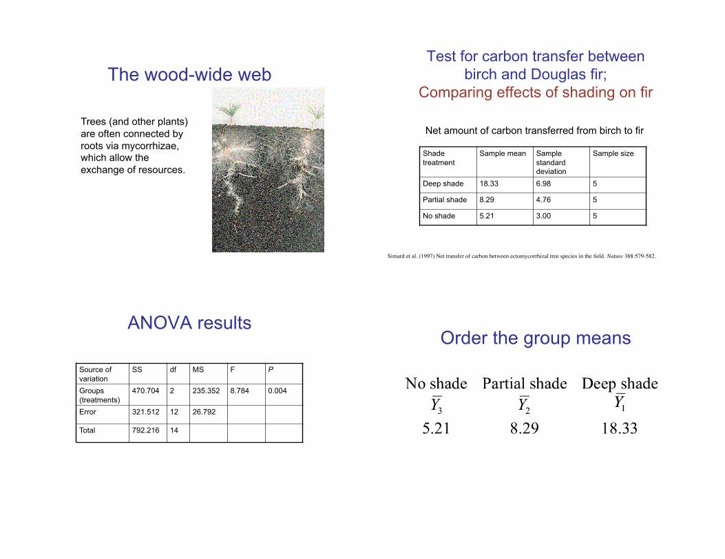
The wood-wide web

Trees (and other plants)

are often connected by

roots via mycorrhizae, which allow the

exchange of resources.

Test for carbon transfer between

birch and Douglas fir;

Comparing effects of shading on fir

Net amount of carbon transferred from birch to fir

Shade

treatment

Sample mean Sample

standard deviation

Sample size

Deep shade 18.33 6.98 5

Partial shade 8.29 4.76 5

No shade 5.21 3.00 5

Simard et al. (1997) Net transfer of carbon between ectomycorrhizal tree species in the field. Nature 388:579-582.!

ANOVA results

Source of

variation

SS df MS F P

Groups

(treatments)

470.704 2 235.352 8.784 0.004

Error 321.512 12 26.792

Total 792.216 14

Order the group means

Null hypotheses for Tukey-Kramer Why not use a series of two-

sample t-tests?

Multiple comparisons would cause the t-tests

to reject too many true null hypotheses.

Tukey-Kramer adjusts for the number of tests.

Tukey-Kramer also uses information about

the variance within groups from all the data,

so it has more power than a t-test with a Bonferroni correction.

Results

Groups which cannot be distinguished share

the same letter.

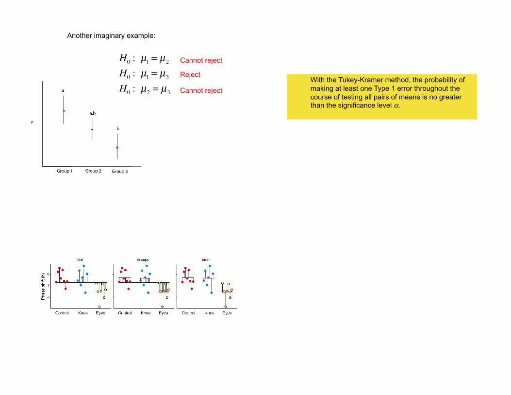
Another imaginary example:

H0: µ

1= µ

2

H0: µ

1= µ

3

H0: µ

2= µ

3

Cannot reject

Cannot reject

Reject With the Tukey-Kramer method, the probability of

making at least one Type 1 error throughout the

course of testing all pairs of means is no greater than the significance level !.