An Integrated PABX/LAN

System Architecture

A thesis submitted to the University of Tasmania in partial fulfilment of the requirement

for the degree of

Master of Technology

bY

Vijayadas Dharmadas Annamalay

Department of Electrical and Electronic Engineering University of Tasmania

Australia December, 1991

ABSTRACT Fast advances in communication engineering especially in the office environment , require an integration of different services and the easy accessibility of these services via smaller and more compact equipment. The integration of voice and data has been the goal of ISDN technology. There is also a high demand for the transfer of high speed data (1.536Mbps e.g. for computer graphics) across different floors and buildings in a typical office environment. One efficient solution for this is to attempt to integrate LAN within an ISDN PABX system. This thesis examines one such design and the proposed design simulation results are also verified here highlighting how the integration of the ISDN PABX & LAN can be achieved succesfully.

Acknowledgements

I would like to extend my sincere gratitude and thanks to the supervisor of my project, Professor DT Nguyen for his immense help and support in enabling me to understand the underlying fundamental concepts involved in the this thesis. I would also like to thank Dr David Lewis for his time and assistance . Finally , I would like to extend my thanks to fellow postgraduate classmates for their support and comments.

Table of Contents

SUMMARY

1. Fundamentals of Digital Transmission

1.1 Standard Telephony 1.2 TDM 1.3 PCM 1.4 Switching Technologies 1.4.1 Circuit Switching 1.4.2 Packet Switching

Page

1-2

3 4 4-5 5 5 6-7

2. ISDN

2.1 ISDN Development 8 2.2 ISDN Services 9-11 2.3 Basic Rate Access 11-13 2.3.1 The Transfer of information 13-15

S/T interface 2.3.2 Synchronization and Frame 15

Alignment (S/T interface)

2.3.3 Frame Alignment U- interface 15-18 2.4 Primary Rate Access 18-20 2.4.1 Frame Alignment 20-21 2.4.2 CRC- Multiframe 21-22 2.5 Micellaneous Functions 23-23 2.6 Layer 2&3 23-24

(Standards V.920 , V.930 series) 2.6.1 Layer 2 24 2.6.2 Transfer of Signalling user-network 24-25 2.6.3 Layer 3 26-27 2.7 Wiring configurations/D channel

monitoring 27

2.7.1 D channel monitoring 27-28 2.8 Point-to-multipoint 28-29 2.9 Point-to-point 29-30

3. LAN

3.1 Standards IEEE 802 31-32 3.2 The connection service

offered by LLC 32-33

3.3 The connectionless service offered by LLC

33

3.4 IBM Token ring 34-37 3.5 Ethernet CSMA/CD 38-42

4. SS7 Signalling system

4.1 Architecture 43-44 4.2 Signalling data link functions 44-45 4.3 Signalling link functions 45-48 4.3.1 Error correction 46 4.3.2 The basic method 46-47 4.3.3 PCR method 47 4.3.4 Error monitoring 47-48 4.3.5 Flow control 48 4.4 Signalling network functions 48--50 4.4.1 Signalling message handling 49 4.4.2 Signalling network management 49-50 4.5 Signalling connection control part 50-51 4.6 ISDN-UP 51-52

5. ISDN PABX & LAN integration

5.1 The PABX 53 5.2 The modern PABX 54-58 5.3 ISDN PABX 58-59 5.4 Integration of ISDN PABX &LAN 59-61

6. Proposed design

6.1 Design onsiderations 62 6.1.1 Terminal communication board 62-63 6.2 The burst switching module 64-67 6.2.1 Line interface circuit(LIF) 65 6.2.2 Polling control circuit(PCC) 65 6.2.3 Module interface circuit 66

6.2.4 Tandem switching unit interface circuit(TIC)

66-67

6.3 Tandem switching unit(TSU) 67-70

7 Simulation and results

7.1 Simulation programs 71 7.1.1 Design for BSM 71-74 7.2 Results for BSM 75-78 7.2.1 Results for BSM 79--82 7.2.2 Simscript program for BSM 83-85 7.3 Design for TSU 86-87 7.3.1 Priority for TSU Traffic 87-88 7.4 Results for TSU 89 7.4.1 90 Acknowledgment packets 7.4.2 Simscript program for TSU 91-94 7.5 Analysis for queuing theory 95-110 7.5.1 Throughput 95 7.5.2 Queuing parameters 96 7.5.3 Balance equations 97-99 7.5.4 Basic equations in queuing theory 99-100 7.5.5 M/M/1 101-105 7.5.6 M/D/1 105-106 7.5.7 M/G/1 107 7.5.8 Verification of simulation results 108-110

8. Discussion

8.1 Number of jobs 111-112 8.2 Design of packet buffer 112--114 8.3 Arrival rates for TSU 114 8.4 Flow control 115-116 8.5 Window control design 116-117 8.5.1 Results for window size

and throughput 118

8.6 Line codes 119 8.7 Delays for BSM and TSU 119 8.8 Transmission delays 120-121

8.9 Proposed addressing scheme 122 8.9.1 Addressing scheme adopted 123 8.10 Application of queuing theory 124-125

Recommendations 126-127

Conclusion 128

References 129-130

SUMMARY This thesis suggests a proposed integrated ISDN PABX/LAN system in accordance with the design specifications in [8]. The concepts of ISDN are developed along with the local area network standards of ethernet and token ring.. The thesis verifies the design results obtained with an emphasis on the use of simulation language simscript version 2.5. The following section will give a breakdown of the contents of the various chapters.

Chapter 1 introduces the fundamentals of digital transmission.. This chapter includes a brief introduction to PCM standard telephony followed by packet and circuit switched technologies.

This is followed by Chapter 2 which gives a summary of the 1.400 standards of both the basic rate and primary rate access standards of ISDN. The descriptions highlight the physical layer, layer 2 and 3 of the ISDN architecture.

Chapter 3, gives some of the essential details in the SS7 signalling system. The descriptions given here are limited to 1-3 MTP levels of the SS7, the SCCP being the 4th level and the ISDN-UP basic and supplementary

services.

Next. Chapter 4 begins with a description of IEEE 802 standards for the token ring and ethernet protocols. The details include the MAC layer set up for different technologies followed by the different services offered by the LLC layer.

Chapter 5, summarizes the design of a modern PABX system. There is then an extension of how a PABX can be upgraded to an ISDN PABX. Some points are also examined as to the integration of an ISDN PABX and

a LAN system.

In Chapter 6, the case-study design used in this thesis [8] is discussed and the new components of the design the 'Burst Switching module' (BSM) and the 'Tandem Switching Unit'(TSU) are discussed here.

Chapter 7 contains information of how the simulation program is written using Simscript version 2.2. Results obtained from the simulation are also attached here. The mathematical analysis which suppports the simulation results is given in section 7.5.

Chapter 8 discusses the results obtained and the delays in the BSM and TSU are also discussed. The transmission delays involved in the overall system are also examined and finally the queuing model is briefly

introduced here for reinforcing the simulation concepts used.

2

Chapter 1: Fundamentals of Digital Transmission

1.1 STANDARD TELEPHONY

The common 'B channel' referred to in the ISDN technology actually refers to a standard digital telephone channel. To fully appreciate the underlying principles of voice transmission, the bit rates for standard digital telephony must be derived.

Voice samples, in a normal telephone conversation , are on average found to reach a maximum frequency in the range of 3400-3800 Hz. Providing extra bandwidth(to prevent aliasing) this value is rounded off to 4KHz. By the sampling theorem, the sampling frequency will then be 4*2 KHz = 8KHz. If voice samples are coded in octets of 8 bits as in pulse code modulation(PCM) techniques, then the bit rate will be 8' 18 = 64kbps .This is the standard bit rate for all voice (B) channels.

Figure 1.2 shows two local exchanges A and B which may belong to towns A and B respectively. In the conventional telephone system, signals from the telephone to the exchange is still in analog form. At the exchange, by a technique using TDM/PCM (which will be explained here) the signals are converted to digital signals and these are then transmitted between the exchanges. One of the challenges of ISDN is to convert the signals from the home to the exchange into digital signals to enhance digital transmission. This can be done by the use of voice codecs, line cards or modems. A more neater solution is to use IVDMs, details of which will be taken up later.

1.2 TDM

The principle of (TDM) or time division multiplexing is commonly used in most digital transmission systems. Bits of information can be packed into fixed 'boxes' referred to as frames and are repeated many times according to the frame time requirement. Referring to the example of the voice 'B' channels, if the sampling frequency is 8KHz, then the frame time will be the reciprocal of the sampling frequency (1 /8kHz) = 0.125ms .If 8 bit sample of consecutive voice channels are contained within this frame, then each bit in the frame takes a timeslot. The principle of timeslots within a frame which repeats itself periodically over a period of time is referred to as 'time division multiplexing'.

1.3 PCM

The (PCM) or pulse code modulation technique is commonly used to convert analog signals into digital signals. In principle, signals are quantized into different levels and the quantized values can then form code words to indicate a digital conversion. Linear quantization is not recommended for voice signals. This is because the signal-to-noise ratio is low for weak signals and high for strong signals. Voice signals are peaky and are weak most of the time. This nature of voice requires the use of log- companding coding technique that provides non-uniform quantization by compressing the signals. This in effect would produce a more desirable signal-to-noise ratio being constant throughout the voice dynamic range.

There are currently two types of compression laws being used for speech signals. The first is the A-law which is more widely used and related to the European standards interface CEPT. The second is the u-law which is related to the North American standards interface Ti.

The techniques described above, produce samples of voice coded in 8 bit sequences. The 8-bit structure can be divided into three sections as shown

4

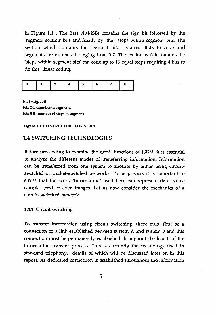
in Figure 1.1 . The first bit(MSB) contains the sign bit followed by the 'segment section' bits and finally by the 'steps within segment' bits. The section which contains the segment bits requires 3bits to code and segments are numbered ranging from 0-7. The section which contains the 'steps within segment bits' can code up to 16 equal steps requiring 4 bits to do this linear coding.

1 I 2 3 4 5 I 6 7 8

bit 1 - sign bit bits 2-4 - number of segments bits 5-8 - number of steps in segments

Figure 1.1: BIT STRUCTURE FOR VOICE

1.4 SWITCHING TECHNOLOGIES

Before proceeding to examine the detail functions of ISDN, it is essential to analyze the different modes of transferring information. Information can be transferred from one system to another by either using circuit-switched or packet-switched networks. To be precise, it is important to stress that the word 'Information' used here can represent data, voice samples ,text or even images. Let us now consider the mechanics of a circuit- switched network.

1.4.1 Circuit switching

To transfer information using circuit switching, there must first be a connection or a link established between system A and system B and this connection must be permanently established throughout the length of the information transfer process. This is currently the technology used in standard telephony, details of which will be discussed later on in this report. As dedicated connection is established throughout the information

5

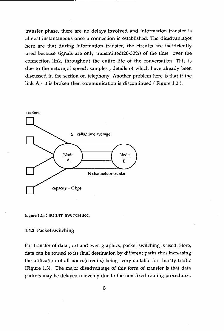
x, calls/time average

N channels or trunks

capacity = C bps

transfer phase, there are no delays involved and information transfer is almost instantaneous once a connection is established. The disadvantages here are that during information transfer, the circuits are inefficiently used because signals are only transmitted(20-30%) of the time over the connection link, throughout the entire life of the conversation. This is due to the nature of speech samples, details of which have already been discussed in the section on telephony. Another problem here is that if the link A - B is broken then communication is discontinued ( Figure 1.2).

stations

Figure 1.2: CIRCUIT SWITCHING

1.4.2 Packet switching

For transfer of data ,text and even graphics, packet switching is used. Here, data can be routed to its final destination by different paths thus increasing the utilization of all nodes(circuits) being very suitable for bursty traffic (Figure 1.3). The major disadvantage of this form of transfer is that data packets may be delayed unevenly due to the non-fixed routing procedures.

6

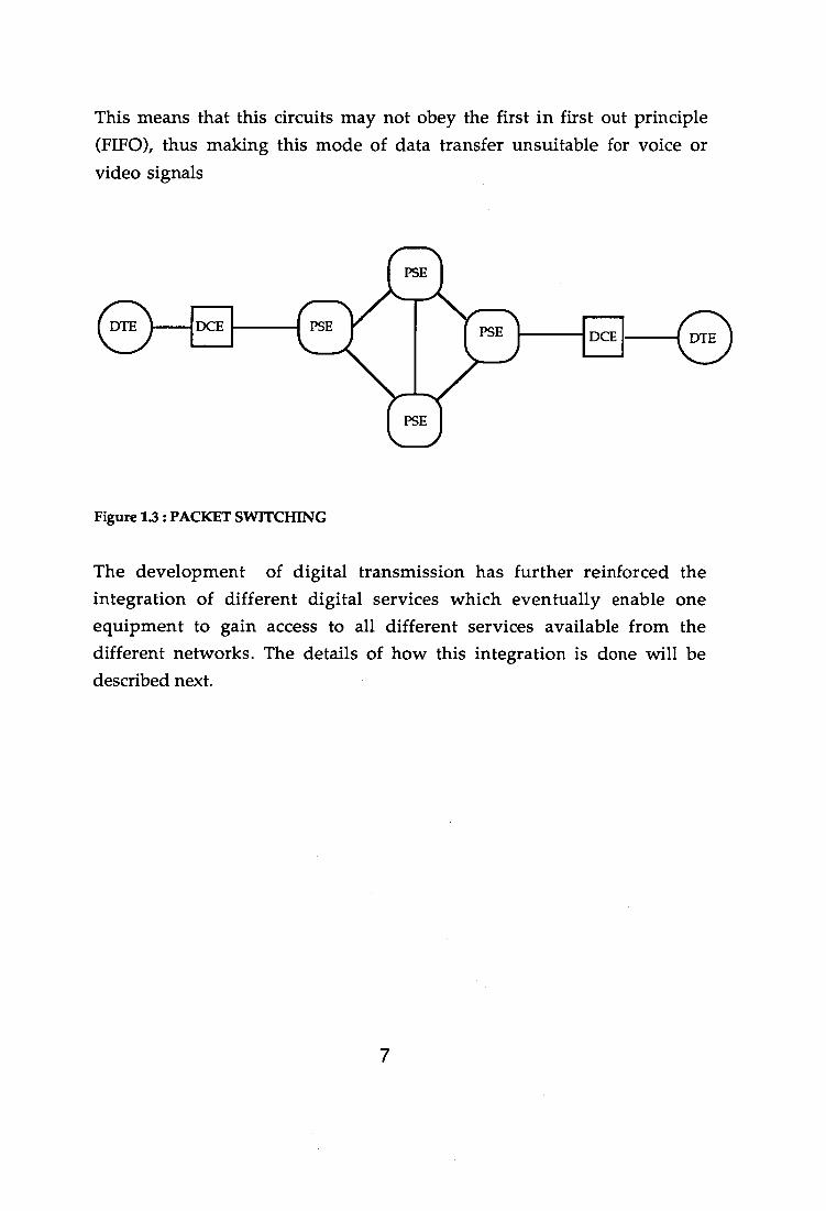
This means that this circuits may not obey the first in first out principle (FIFO), thus making this mode of data transfer unsuitable for voice or video signals

Figure 1.3 : PACKET SWITCHING

The development of digital transmission has further reinforced the integration of different digital services which eventually enable one equipment to gain access to all different services available from the different networks. The details of how this integration is done will be described next.

7

CSN

OTHER

NETWORKS

Chapter 2 : ISDN

2.1 ISDN DEVELOPMENT

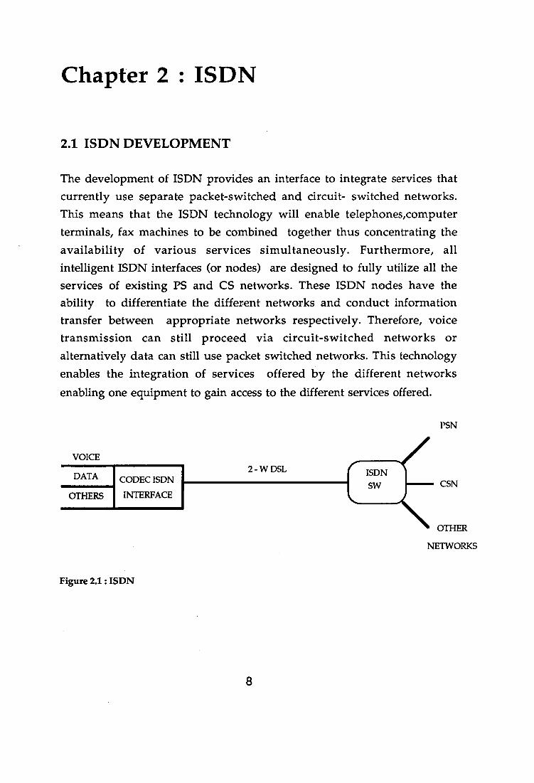
The development of ISDN provides an interface to integrate services that currently use separate packet-switched and circuit- switched networks. This means that the ISDN technology will enable telephones,computer terminals, fax machines to be combined together thus concentrating the availability of various services simultaneously. Furthermore, all intelligent ISDN interfaces (or nodes) are designed to fully utilize all the services of existing PS and CS networks. These ISDN nodes have the ability to differentiate the different networks and conduct information transfer between appropriate networks respectively. Therefore, voice transmission can still proceed via circuit-switched networks or alternatively data can still use packet switched networks. This technology enables the integration of services offered by the different networks

enabling one equipment to gain access to the different services offered.

PSN

VOICE

DATA

OTHERS

CODEC ISDN INTERFACE

2- W DSL

Figure 2.1 : ISDN

2.2 ISDN SERVICES

As explained, ISDN attempts to integrate both packet-switched data and circuit-switched voice services. To efficiently achieve this integration, two media or channels of information transfer are defined in this technology. The first being the 'B' channel which is utilized in circuit switched telephone connections, transferring samples of voice. The bit rate of the voice channels can be calculated (which will be indicated in the section that deals with telephony) to be 64kbps. The B channels can also be used to transfer data packets utilizing the circuit switched circuits at a rate of 64kbps.

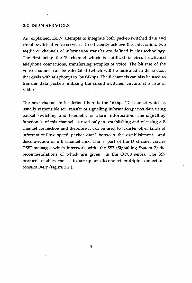
The next channel to be defined here is the 16kbps 'D' channel which is usually responsible for transfer of signalling information,packet data using packet switching and telemetry or alarm information. The signalling function 's' of this channel is used only in establishing and releasing a B channel connection and therefore it can be used to transfer other kinds of information(low speed packet data) between the establishment and disconnection of a B channel link. The 's' part of the D channel carries DSSI messages which interwork with the SS7 (Signalling System 7) the recommendations of which are given in the Q.700 series. The SS7 protocol enables the 's' to set-up or disconnect multiple connections consecutively (Figure 2.2).

9

B1

ISDN

access

ISDN TERM ISDN TERM

Figure 2.2 : ISDN COMMUNICATION SCENARIO

The next function of the D channel is the 'p' sub-section which is responsible for the transfer of data using the packet switching. This sub-section can support low speed data transfer(eg. X.25). The last function of the D channel is the 't' sub-section also utilized for very low speed data(eg. telemetry/alarm information). The overall bit rate of the D channel will be specified according to the different services being offered.

The access offered by ISDN can be characterized into two groups. The first being the basic rate access and the second being the primary rate access.These two access will be discussed separately. For clarity purposes, each of these services is systematically described according to the standards released by CCITT in 1988(Blue Book). For standardization purposes, each access is divided into three layers, according to the OSI model, starting with first layer which is the physical layer, the second layer being data link layer and the final layer being the network layer. The details that follow for the physical layer will be obtained from standards 1.400 series. This will

10

. Isdn access node

B2

B1

be followed by some information for the data link and network layers. All information being taken from the Q.920 and Q.930 series respectively.

2.3 BASIC RATE ACCESS

This service access is the first access available in ISDN and must be clearly understood for the appreciation of different interfaces involved in ISDN. This access offers the use of two B channels each having a bit rate of 64kpbs and a D channel having the bit rate of 16kbps. The net bit rate thus becomes 144kbps. However, another 48kbps is added to this figure for additional synchronization , framing etc to give a value of 192kbps.

Each voice sample is digitized to 8 bits and due to the nature of voice, the sampling frequency is 8kHz giving 64kbps per voice channel. This information will later be used to verify the standard bit rate of 192kbps in the section which deals with the frame structure as specified by the physical layer standard from the V 1.430 series[1,13].

11

TA

TEl ET NT2 LT NT1

4W 4W 2W

1■1•

TA

S INTERFACE T INTERFACE

R INTERFACE

BASIC RATE

ACCESS

U INTERFACE

TEl

V INTERFACE

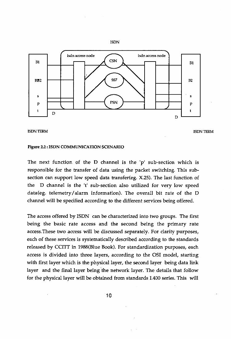
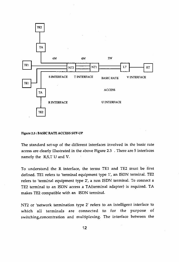
Figure 2.3 : BASIC RATE ACCESS SET-UP

The standard set-up of the different interfaces involved in the basic rate access are clearly illustrated in the above Figure 2.3 . There are 5 interfaces namely the R,S,T U and V.

To understand the R interface, the terms TEl and TE2 must be first defined. TEl refers to 'terminal equipment type 1', an ISDN terminal. TE2 refers to 'terminal equipment type 2', a non ISDN terminal. To connect a TE2 terminal to an ISDN access a TA(terminal adapter) is required. TA makes TE2 compatible with an ISDN terminal.

NT2 or 'network termination type 2' refers to an intelligent interface to which all terminals are connected to for the purpose of switching,concentration and multiplexing. The interface between the

12

terminals and NT2 is referred to as the S interface.

NT1 or 'network termination1 1 refers to the termination of the subscriber(or user) loop and performs the physical and electromagnetic termination. The interface between NT2 and NT1 is referred to as the T interface.

This is followed by LT or 'line termination' which provides the terminations of the subscriber line which carries information in the duplex mode to and from the terminals. ' ET an 'exchange termination' usually refers to the function of the central office providing the network services.The interface between NT1 and LT is referred to as the 'U' interface and between LT and ET, the 'V' interface. This completes the definitions of Figure 2.3 for the basic access interfaces.

In the following sections, the terms TE and NT will be used (according to V 1.400 series) to explain how information transfer takes place between all these interfaces. The term TE will refer to the 'terminal termination layerl' of the physical layer covering all aspects of TEl , TA and NT2 functional groups. The term NT will refer to the 'network termination layer1' of the physical layer covering all aspects of NT1 and NT2 functional groups.

2.3.1 The transfer of information S/T interface

The standards have specified frame formats for the transfer of information across the existing networks. All information for the physical layer will be -packed into a frame containing 48 bits in directions TE-NT or NT-TE for the SIT interface.

13

BITS

1-24

(B1-CHN & B2-CHN) 1ST OCTET + OVERHD

BITS

25-48

(B1-CHN & B2-CHN)

2ND OCTET + OVERHD

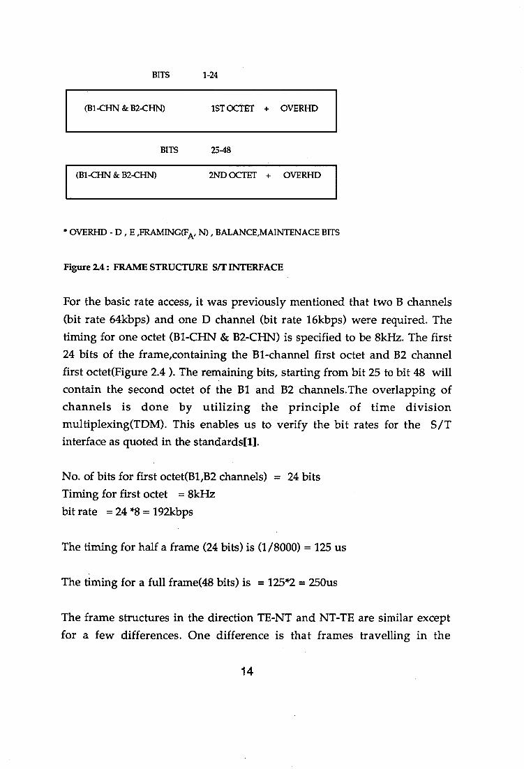
* OVERHD - D, E ,FRAMING(FA, , BALANCE,MAINTENACE BITS

Figure 2.4: FRAME STRUCTURE S/T INTERFACE

For the basic rate access, it was previously mentioned that two B channels (bit rate 64kbps) and one D channel (bit rate 16kbps) were required. The timing for one octet (B1-CHN & B2-CI-IN) is specified to be 8kHz. The first 24 bits of the frame,containing the B1-channel first octet and B2 channel first octet(Figure 2.4). The remaining bits, starting from bit 25 to bit 48 will contain the second octet of the B1 and B2 channels.The overlapping of channels is done by utilizing the principle of time division multiplexing(TDM). This enables us to verify the bit rates for the SIT interface as quoted in the standards[1].

No. of bits for first octet(B1,B2 channels) = 24 bits Timing for first octet = 8kHz bit rate = 24 *8 = 192kbps

The timing for half a frame (24 bits) is (1/8000) = 125 us

The timing for a full frame(48 bits) is = 125 3'2 = 250us

The frame structures in the direction TE-NT and NT-TE are similar except for a few differences. One difference is that frames travelling in the

14

direction NT-TE have a bit referred to as the D-echo channel bit the function of which will be described later.

2.3.2 Synchronization and frame alignment(S/T interface)

It is very essential that frames adhere to their timing requirement. To do this, a network clock times all frames travelling in the NT-TE direction. All outgoing frames from TE-NT are delayed by 2 bits with respect to the incoming frames from NT.

The next important concept is that of frame Alignment. There are different coding systems used for the S,T interfaces and the U interface , details of which will be described later. For the S,T interfaces, the coding used is the psuedo-ternary AMI (Alternate Mark Inversion) coding where a binary zero represents a positive or negative pulse (alternating in polarity) also known as a 'mark' and a binary one represents no pulse condition also known as a 'space'. If the polarity of two consecutive zeros are the same , then a bipolar violation is said to occur. A set of pulses occurring at the beginning of the frame and within the first 14 or 13 bits of the frame will result in a violation.These violations assist in the frame alignment procedure and frame alignment is said to occur when three consecutive pairs of these violations are detected.

2.3.3 Frame alignment U-interface

Amongst the S,T and U interfaces, the U interface is the farthest interface. After much research and discussion, the solution adopted for coding the signal on U interface by ANSI in 1988(later by CCITT) is the 2B1Q standard. This coding enables a reduction in the bandwidth required for transmission providing a better immunity to crosstalk- a very common occurrence in transmission systems. This coding is also favorable for more efficient modes of synchronization.

15

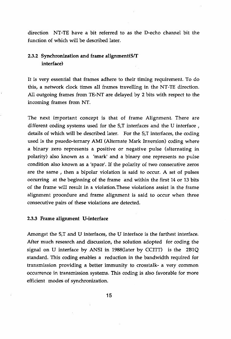
The 2B1Q uses the di-bit concept and combines two consecutive bits of form a symbol(QUAT). There are four possible outcomes in the two bits [00,01,10,11]. To establish a one to one correspondence between the four values and the symbols, the 2 bits are divided into 'bitl' and 'bit2' positions. The first bit is referred to as a sign bit and the second bit the magnitude bit. Using the signs '+' , '-' and numbers '3','1', the following table can be produced.

First bit Second bit Quat Symbol 1 0 +3 1 1 +1 0 1 -1 0 0 -3

The bit rate at this interface with 2B channels(64kpbs each), D channel(16kpbs) and 16kpbs for framing and maintenance, is 160kpbs. Converting this figure to the baud or symbol rate, this becomes 160/2 = 80kbauds/s , since there are two bits to a symbol.

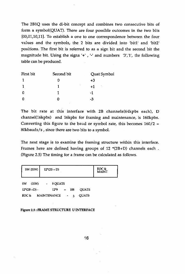
The next stage is to examine the framing structure within this interface. Frames here are defined having groups of 12 *(2B+D) channels each . (Figure 2.5) The timing for a frame can be calculated as follows.

SW (ISW) 12*(2B + D) EOC & MAINT

SW (ISW) - 9 QUATS

12*(2B +D) - 12*9 = 108 QUATS

EOC & MAINTENANCE - 3 QUATS

Figure 2.5 : FRAME STRUCTURE U INTERFACE

16

Timing for one group of (2B + D) channels is 1/8 * 10 = 0.125ms Timing for 12 groups of(2B +D) channels is = 0.125*12 = 1.5ms

To further enhance secure framing, there are SW(or sync word) at the beginning and a maintenance channel at the end of each frame. The SW or syncword (or ISW) is a sequence of 9Quats defined as follows : (+3 +3 -3 -3 -3 +3 -3 +3 +3) and they must appear before each frame as shown in Figure 2.5.

The number of quats within each frame can be calculated as follows:

number of Quats in SW = 9Quats

number of Quats in 12(2B + D)channel = (9*12)Quats = 108 Quats

number of Quats in maintenance channel = 6bits/2 = 3Quats

Total = 9 + 108 + 3 = 120 Quats

There are therefore 120 Quats in each frame structure.

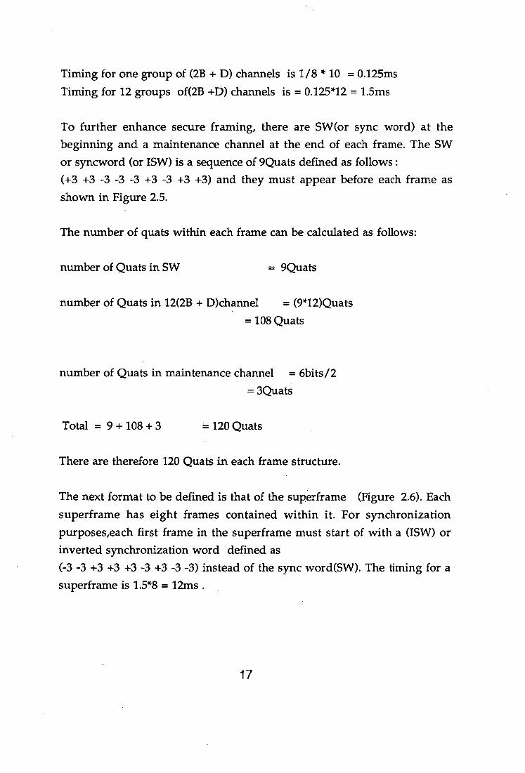
The next format to be defined is that of the superframe (Figure 2.6). Each superframe has eight frames contained within it. For synchronization purposes,each first frame in the superframe must start of with a (ISW) or inverted synchronization word defined as (-3 -3 +3 +3 +3 -3 +3 -3 -3) instead of the sync word(SW). The timing for a superframe is 1.5*8 = 12ms .

17

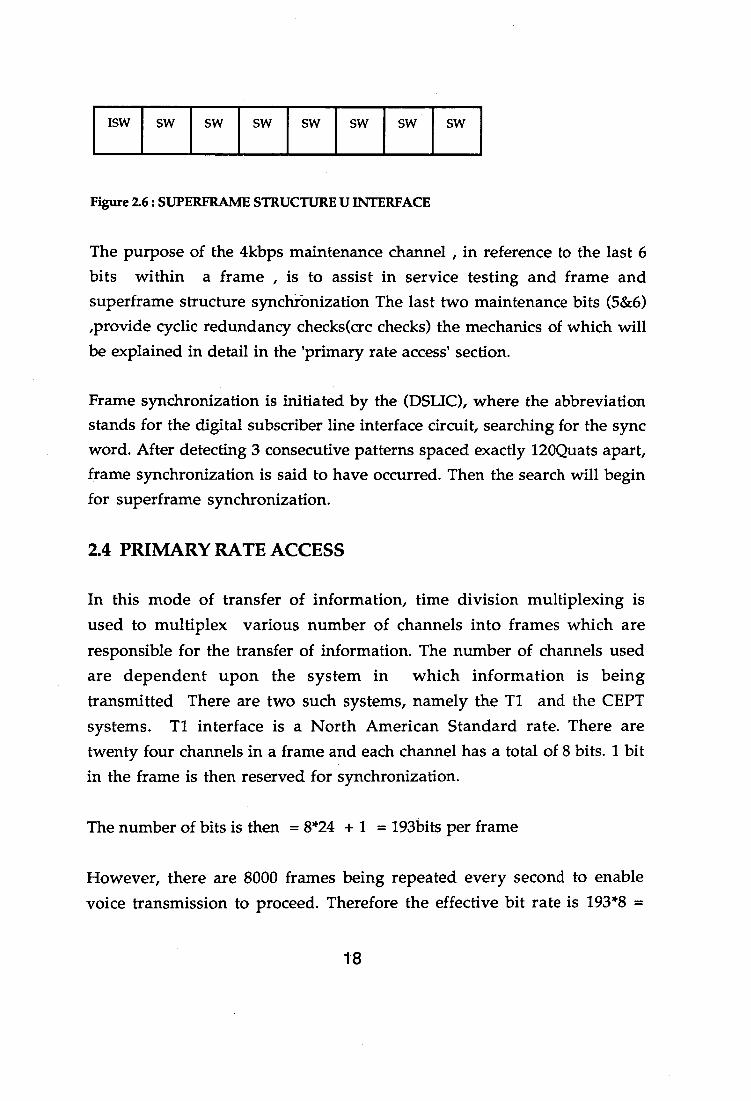
ISW SW SW SW SW SW SW SW

Figure 2.6: SUPERFRAME STRUCTURE U INTERFACE

The purpose of the 4kbps maintenance channel , in reference to the last 6 bits within a frame , is to assist in service testing and frame and superframe structure synchronization The last two maintenance bits (5&6) ,provide cyclic redundancy checks(crc checks) the mechanics of which will be explained in detail in the 'primary rate access' section.

Frame synchronization is initiated by the (DSLIC), where the abbreviation stands for the digital subscriber line interface circuit, searching for the sync word. After detecting 3 consecutive patterns spaced exactly 120Quats apart, frame synchronization is said to have occurred. Then the search will begin for superframe synchronization.

2.4 PRIMARY RATE ACCESS

In this mode of transfer of information, time division multiplexing is used to multiplex various number of channels into frames which are responsible for the transfer of information. The number of channels used are dependent upon the system in which information is being transmitted There are two such systems, namely the Ti and the CEPT systems. Ti interface is a North American Standard rate. There are twenty four channels in a frame and each channel has a total of 8 bits. 1 bit in the frame is then reserved for synchronization.

The number of bits is then = 8*24 + 1 = 193bits per frame

However, there are 8000 frames being repeated every second to enable voice transmission to proceed. Therefore the effective bit rate is 193*8 =

18

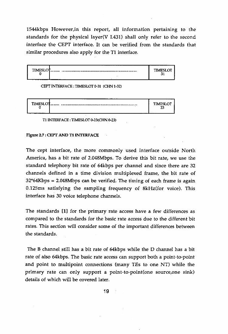
1544kbps However,in this report, all information pertaining to the standards for the physical layer(V 1.431) shall only refer to the second interface the CEPT interface. It can be verified from the standards that similar procedures also apply for the Ti interface.

TIMESLO-

TIMESLOT 31

CEPT INTERFACE : TIMESLOT 0-31 (CHN 1-32)

TIMESLO7 0

TIMESLOT 23

Ti INTERFACE : TIMESLOT 0-23(CHN 0-23)

Figure 2.7 : CEPT AND Ti INTERFACE

The cept interface, the more commonly used interface outside North America, has a bit rate of 2.048Mbps. To derive this bit rate, we use the standard telephony bit rate of 64kbps per channel and since there are 32 channels defined in a time division multiplexed frame, the bit rate of 32*64Kbps = 2.048Mbps can be verified. The timing of each frame is again 0.125ms satisfying the sampling frequency of 8kHz(for voice). This interface has 30 voice telephone channels.

The standards [1] for the primary rate access have a few differences as compared to the standards for the basic rate access due to the different bit rates. This section will consider some of the important differences between the standards.

The B channel still has a bit rate of 64kbps while the D channel has a bit rate of also 64kbps. The basic rate access can support both a point-to-point and point to multipoint connections (many TEs to one NT) while the primary rate can only support a point-to-point(one source,one sink) details of which will be covered later.

19

For the basic rate access, it is possible to deactivate the TE to remain in a low power consumption mode if there is no information transfer. However, for the primary rate access, the user-network interface must be always active because of the continuous flow of data and high bit rates.

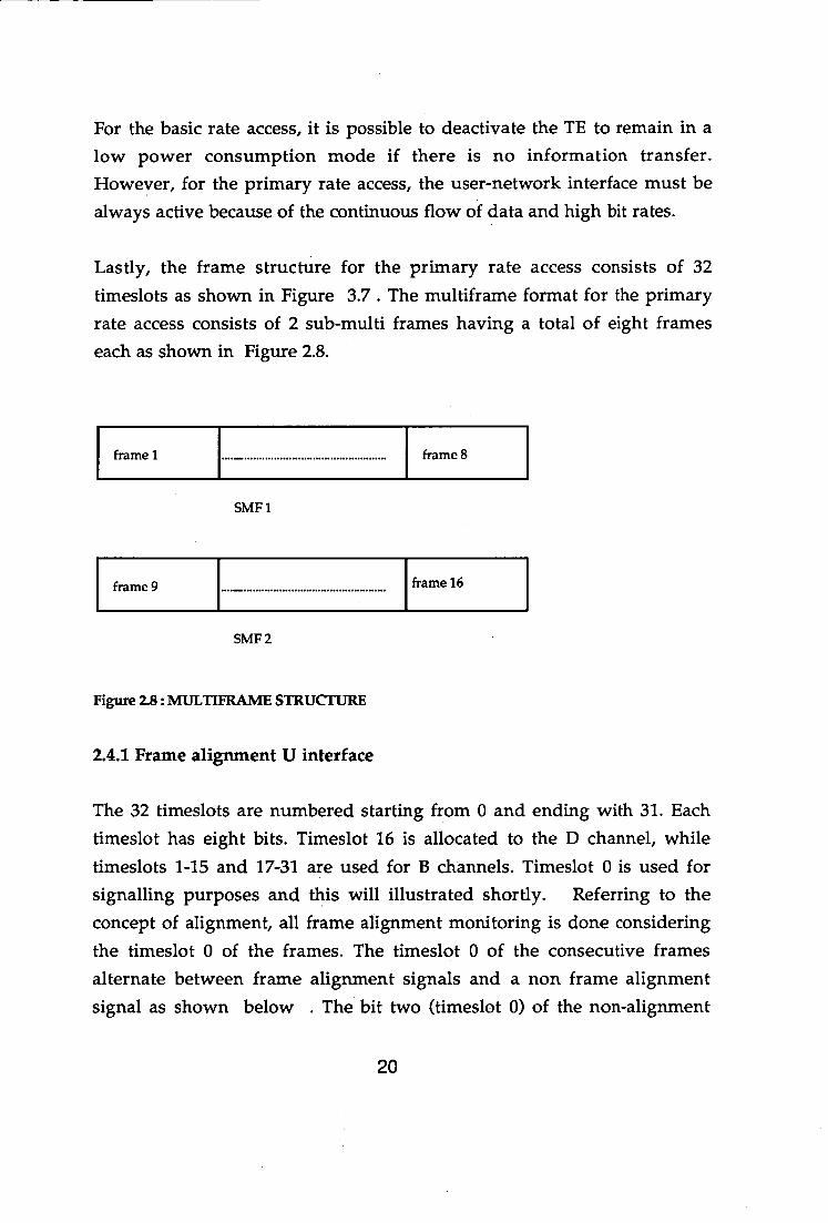
Lastly, the frame structure for the primary rate access consists of 32 timeslots as shown in Figure 3.7. The multiframe format for the primary rate access consists of 2 sub-multi frames having a total of eight frames each as shown in Figure 2.8.

frame 1

frame 8

SMF 1

frame 9

frame 16

SMF 2

Figure 2.8 : MULTIFRAME STRUCTURE

2.4.1 Frame alignment U interface

The 32 timeslots are numbered starting from 0 and ending with 31. Each timeslot has eight bits. Timeslot 16 is allocated to the D channel, while timeslots 1-15 and 17-31 are used for B channels. Timeslot 0 is used for signalling purposes and this will illustrated shortly. Referring to the concept of alignment, all frame alignment monitoring is done considering the timeslot 0 of the frames. The timeslot 0 of the consecutive frames alternate between frame alignment signals and a non frame alignment signal as shown below . The bit two (timeslot 0) of the non-alignment

20

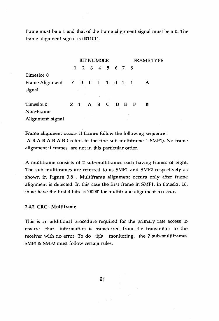
frame must be a 1 and that of the frame alignment signal must be a 0. The frame alignment signal is 0011011.

BIT NUMBER FRAME TYPE 1 2 3 4 5 6 7 8

Timeslot 0 Frame Alignment Y 0 0 1 1 0 1 1 A signal

Timeslot 0

Z 1 ABCDEF B Non-Frame Alignment signal

Frame alignment occurs if frames follow the following sequence : ABABABAB( refers to the first sub multiframe 1 SMF1). No frame

alignment if frames are not in this particular order.

A multiframe consists of 2 sub-multiframes each having frames of eight. The sub multiframes are referred to as SMF1 and SMF2 respectively as shown in Figure 3.8 . Multiframe alignment occurs only after frame alignment is detected. In this case the first frame in SMF1, in timeslot 16, must have the first 4 bits as '0000' for multiframe alignment to occur.

2.4.2 CRC - Multiframe

This is an additional procedure required for the primary rate access to ensure that information is transferred from the transmitter to the receiver with no error. To do this monitoring, the 2 sub-multiframes SMF! & SMF2 must follow certain rules.

21

FRAME NUMBER 0 1 2 3 4 5 6 7 8 9 10 11 12 13 14 15 Y1 Y2 Y3 Y4 Y1 Y2 Y3 Y4

Z1 Z2 Z3 Z4 Z5 Z6 Z7 Z8

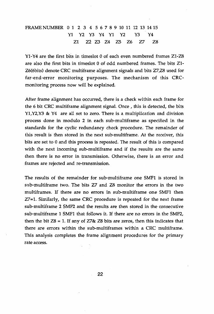
Y1-Y4 are the first bits in timeslot 0 of each even numbered frames Z1-Z8 are also the first bits in timeslot 0 of odd numbered frames. The bits Z1- Z6(6bits) denote CRC multiframe alignment signals and bits Z7,Z8 used for far-end-error monitoring purposes. The mechanism of this CRC-monitoring process now will be explained.

After frame alignment has occurred, there is a check within each frame for the 6 bit CRC multiframe alignment signal. Once , this is detected, the bits Y1,Y2,Y3 & Y4 are all set to zero. There is a multiplication and division process done in modulo 2 in each sub-multiframe as specified in the standards for the cyclic redundancy check procedure. The remainder of this result is then stored in the next sub-multiframe. At the receiver, this bits are set to 0 and this process is repeated. The result of this is compared with the next incoming sub-multiframe and if the results are the same then there is no error in transmission. Otherwise, there is an error and frames are rejected and re-transmission.

The results of the remainder for sub-multiframe one SMF1 is stored in sub-multiframe two. The bits Z7 and Z8 monitor the errors in the two multiframes. If there are no errors in sub-multiframe one SMF1 then Z7=1. Similarly, the same CRC procedure is repeated for the next frame sub-multiframe 2 SMF2 and the results are then stored in the consecutive sub-multiframe 1 SMF1 that follows it. If there are no errors in the SMF2, then the bit Z8 = 1. If any of Z7& Z8 bits are zeros, then this indicates that there are errors within the sub-multiframes within a CRC multiframe. This analysis completes the frame alignment procedures for the primary rate access.

22

2.5 MISCELLANEOUS FUNCTIONS

There are other interface functions defined for both the primary rate and basic rate access in the CCITT standards. There are stipulations for two separate circuits one used for transmission and the other used for receiving signals. The purpose for this is to reduce the distortion of signals due to noise and echoes. Echoes occur in a transmission media due to a non-uniform distribution of impedance along the transmission line ,the theory of which can be obtained from the 'analysis of echoes' in 'transmission lines and circuits'. After much research, the final solution adopted to solve this problem was to add a hybrid and a echo cancellor(linear and non linear) within a terminal equipment.There are also specifications within the standards for loopbacks. Loopbacks are mainly required for testing purposes. There are two kind of loopbacks defined in the standards. They are the transparent and non-transparent loopbacks. When transparent loopbacks are activated, 100% of the transmission information is looped back. In the non-transparent case this is not so. Loopbacks can also be used to check the integrity of the line interface circuits and network interface circuits operating at the various ISDN interfaces.There is also a provision in checking the performance of the higher layers i.e. data link ,network etc.

The other details within the physical layer standards include detailed specifications on the line and power configurations. There are also specifications on the maximum allowable atttenuations along with details of how the effects of 'wander' and 'jitter' can be prevented. This details of the wiring configurations will be covered shortly. Details of the D-channel mechanism will also be dealt with

2.6 LAYER 2 & 3 (STANDARDS V 920 ,V930 SERIES)

The previous sections have briefly covered some of the relevant points pertaining to the CCITT standards of the physical layer for both the basic

23

and primary rate accesses. This section is a follow up, as it will cover the structure and functions of layers 2 and 3 in relation to the OSI architecture.

2.6.1 Layer 2

The layer 2(data link layer) of the ISDN architecture, utilizes the Link Access Protocols for its signalling functions on the D-channel. The abbreviation for this is LAPD and is based on similar recommendations of the LAPB(Balanced Link Access Protocol). The LAPB procedures are defined in detail in the standards for the packet switching user-network interface of the X.25. Both the LAPD and LAPB are subsets of the ABM(Asynchronous Balanced Mode) of transmission. The ABM in turn is a subset of the HDLC(high data level control). Having this common similarities , it becomes much easier to integrate the packet switching standards into the ISDN technology without having to set all list of new standards for the packet mode of transmission within ISDN.

For illustration purposes, the terms user and network interfaces will be used here. The user interface corresponds to the customer premises being the equivalent of the R,S,T interfaces. The network interface will correspond to the U interface.

2.6.2 Transfer of signalling user-network

When a user equipment is introduced at the customer premises, three parameters are defined to enable information flow. The first is the TEl or terminal endpoint identifier. If the user equipment belongs to the automatic TEl assignment category, then the network will assign a TEl value for the user equipment. If the user belongs to the non-automatic category, the TEl value must be entered into the user-equipment.

The second parameter is the SAPI or service access point identifier. The SAPI is used to identify the service access point on the network or the user

24

side of the user-network interface. The third parameter is the CES or connection endpoint suffix established in the layer 3 or management entity to address the data link layer.

Having established these parameters, the data link layer (layer 2) that establishes its own identifier, DLCI or the data link connection identifier defined as the sum of the TEl and the SAFI as indicated;DLCI = TEl + SAPI. This DLCI is only known by the data link layer and remains non-existent to the layer 3 entity.

A corresponding identifier, the CEI or connection endpoint identifier is established in the layer 3 or management entity. The CEI is a sum of the SAFI and the CES : CEI = SAPI + CES .

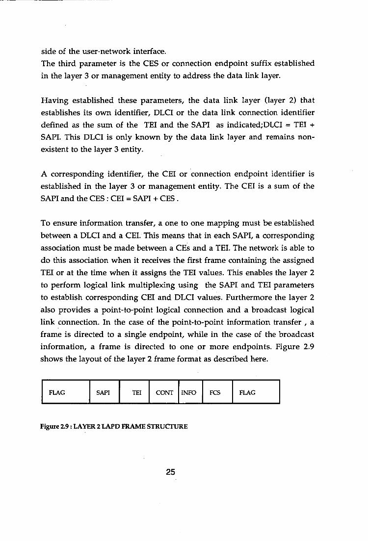
To ensure information transfer, a one to one mapping must be established between a DLCI and a CEI. This means that in each SAPI, a corresponding association must be made between a CEs and a TEI. The network is able to do this association when it receives the first frame containing the assigned TEl or at the time when it assigns the TEl values. This enables the layer 2 to perform logical link multiplexing using the SAFI and TEl parameters to establish corresponding CEI and DLCI values. Furthermore the layer 2 also provides a point-to-point logical connection and a broadcast logical link connection. In the case of the point-to-point information transfer , a frame is directed to a single endpoint, while in the case of the broadcast information, a frame is directed to one or more endpoints. Figure 2.9 shows the layout of the layer 2 frame format as described here.

FLAG SAP! TEl CONT INFO FCS FLAG

Figure 2.9 : LAYER 2 LAPD FRAME STRUCTURE

25

2.6.3 Layer 3

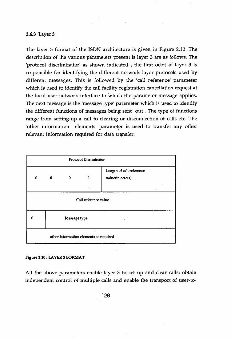
The layer 3 format of the ISDN architecture is given in Figure 2.10 .The description of the various parameters present is layer 3 are as follows. The 'protocol discriminator' as shown indicated , the first octet of layer 3 is responsible for identifying the different network layer protocols used by different messages. This is followed by the 'call reference' parameter which is used to identify the call facility registration cancellation request at the local user-network interface to which the parameter message applies. The next message is the 'message type' parameter which is used to identify the different functions of messages being sent out . The type of functions range from setting-up a call to clearing or disconnection of calls etc. The 'other information elements' parameter is used to transfer any other relevant information required for data transfer.

Protocol Disriminator

0 0 0 0

Length of call reference

value(in octets)

Call reference value

0 Message type

other information elements as required

Figure 2.10 : LAYER 3 FORMAT

All the above parameters enable layer 3 to set up and clear calls; obtain independent control of multiple calls and enable the transport of user-to-

26

user information. Besides theses, the layer 3 functions also include the notification of interworking and the delivery of the calling number. All these facilities are further enhanced by the usage of the SS7 signalling system which will be described chapter 4.

2.7 WIRING CONFIGURATIONS/D CHANNEL MONITORING

This section will examine the different wiring arrangements possible for an ISDN network(i.e. the customer premises).The primary rate access can support the point-to-point configuration while the basic rate access can support both the point-to-point and also a point-to-multipoint configuration.

2.7.1 D- channel monitoring

To understand how the basic rate access can support a point-to-multipoint configuration, it is first important to understand the D-channel procedures inherent here. Referring to the frame formats in the direction from TE-NT , after every B channel octet, there is an D channel bit. Comparing this with the frame format in the direction NT-TE, after every B octet, there is an E bit referred to as the D-echo channel. The D-echo bit also provides a collision detection mechanism. While transmitting information on the D channel,TEs also monitor the received D-echo channel bit and compare the last transmitted bit with the next available D-echo bit. If transmitted bit and echo bit are the same,TEs will continue transmission. If different, TEs will cease transmission immediately and will monitor the D-echo channel bit. If the TEs have no layer 2 frames to send' they will send binary ones on the D channel. If the NT has no layer 2 frames to send, it will send all binary ones or repetitions of the octet 01111110.

This mechanism enables the different TEs connected to gain access to the D channel, in a point-to-multipoint arrangement. To do this , all TEs are

27

assigned different classes for different messages and each class is then assigned either a 'high' or 'low' priority value. All signalling information are given are higher class ranking as compared to other types of information. All TEs must use the facilities of the D channel to transfer information. Before the transfer of data all the priority values are in the 'high' state. The instant a TE gains access and uses the facilities of the D channel, its priority is changed from high to low, within the class that the data was sent in, and remains low until all other TEs have had a chance to use the facilities of the D channel. For example, if there are eight TEs using the services of the D channel and if one terminal equipment uses the D channel, its priority is reduced immediately. to a lower priority value. This is done systematically for all the other TEs until such time that all have had the chance to transmit frames over the D channel. The priority level of the TEs are increased to the high priority level and the pattern is repeated again ensuring that every TE always gets a chance to use the D channel and no blocking prevails.

2.8 POINT-TO-MULTIPOINT

The distances in a point-to-multipoint configuration are controlled by the maximum round trip delay involved due to the E bits being reflected back towards the TEs. Another consideration is that of attenuation of signals. The first factor is more relevant to the point-to-multipoint case as maximum of 8 TEs can be connected in this way and the total round trip delay for the reflected bits would be significant as distances increase..

The above arrangement can either support the short-passive bus or the extended bus configuration. The short passive bus configuration can have a operational distance of 100m with a low impedance of 75 ohms. It can support a maximum of 8 TE having a spacing of 10m between each of them. Another possible arrangement is the extended passive bus arrangement. Figures 2.11 & 2.12 indicate the possible layouts described here.

28

0 0 0 0 0 0 0 TE TE TE TE TE TE TE

Figure 2.11 : SHORT PASSIVE BUS

Figure 2.12 : EXTENDED PASSIVE BUS

2.9 POINT-TO-POINT

For the point-to-point configuration, the distances involved depend on both the maximum round trip delay and also the attenuation.The maximum distance between a source and a sink is kept at lkm. This distance criteria ensures that the maximum round delays are not excessive and signals are not badly attenuated (Figure 2.13 ).

29

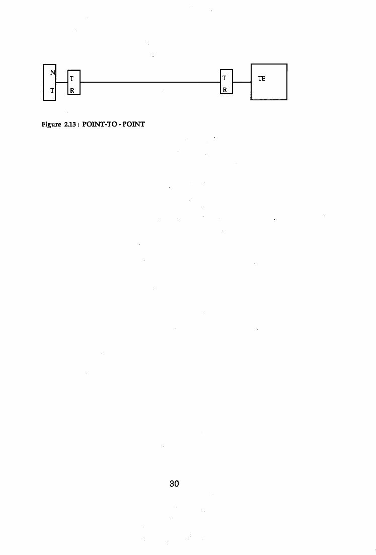
Figure 2.13: POINT-TO - POINT

30

Chapter 3 : LANs

3.1 IEEE 802 STANDARDS

Having obtained a understanding of the ISDN standards, it is now essential to understand some of the underlying principles and standards governing the local area network(LANs). This section will concentrate on the two main kinds of local area networks i.e. the token ring complying with the IEEE 802.5 [16] and the ethernet with the IEEE 802.3 standards[15].

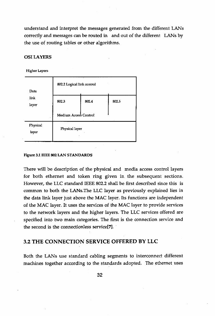
For both the token ring and the ethernet, the IEEE standards specify the requirements for all the OSI equivalent of the physical and data link layers. The data link layer is seen to comprise of two elements, the first being the medium access control or the MAC layer and this is followed by the logical link layer LLC. While the specifications for the physical layer and the MAC layer for both the ethernet and token ring differ, it must be pointed out that the logical link control designs for both the LANs adhere very closely to the IEEE standards 802.2[14]. The reason for this is as follows. The second layer of the OSI forms the data link layer of the OSI architecture. This means that it two systems are to communicate, data will be passed through the link layer from one system to the other. The complication arises if two systems adopt different standards for the physical and the MAC layers. In this case, it becomes essential to define a common standard which would be within the data link layer and be able to accommodate the different protocols utilized by the physical and MAC layers. To enable two different systems like the ethernet and token ring, a common LLC (logical link control) design must be adopted for the LLC layers within the two LANs. The LLC standards can be obtained from the IEEE 802 specifications. (Figure 3.1) This enables a gateway to be attached at the connection points between two LANs . The gateway is then able to

31

understand and interpret the messages generated from the different LANs correctly and messages can be routed in and out of the different LANs by the use of routing tables or other algorithms.

OSI LAYERS

Higher Layers

802.2 Logical link control

Data

link 802.3

802.4

802.5 layer

Medium Access Control

Physical layer Physical layer

Figure 3.1 IEEE 802 LAN STANDARDS

There will be description of the physical and media access control layers for both ethernet and token ring given in the subsequent sections. However, the LLC standard IEEE 802.2 shall be first described since this is common to both the LANs.The LLC layer as previously explained lies in the data link layer just above the MAC layer. Its functions are independent of the MAC layer. It uses the services of the MAC layer to provide services to the network layers and the higher layers. The LLC services offered are specified into two main categories. The first is the connection service and the second is the connectionless service[7].

3.2 THE CONNECTION SERVICE OFFERED BY LLC

Both the LANs use standard cabling segments to interconnect different machines together according to the standards adopted. The ethernet uses

32

the standard cable segments and repeaters as specified by 802.3 to interconnect different sections of ethernet together.. In this situation, the service provided by the LLC is referred to as a 'connection service'. In other words, if two segments of the same LANs are interconnected by their standard physical media, this then defines a connection service. The error recovery mechanism are based on ABM mode of HDLC. The medium access control or (MAC) provides a bit error detection capability by using the FCS or frame check sequence at the end of each frame. If errors are detected, they are passed up to the logical link control or higher layers for action. The responsibility of correcting the errors detected by the FCS can be assigned to the LLC or the higher layers.

3.3 THE CONNECTIONLESS SERVICE OFFERED BY LLC

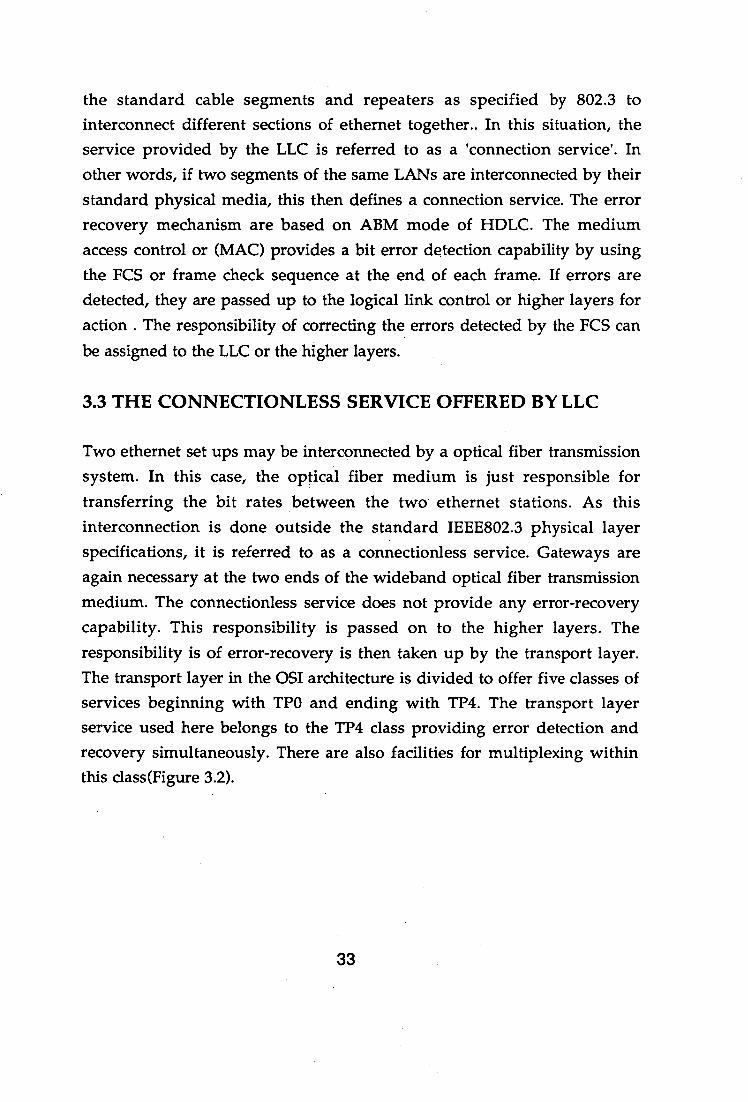
Two ethernet set ups may be interconnected by a optical fiber transmission system. In this case, the optical fiber medium is just responsible for transferring the bit rates between the two ethernet stations. As this interconnection is done outside the standard IEEE802.3 physical layer specifications, it is referred to as a connectionless service. Gateways are again necessary at the two ends of the wideband optical fiber transmission medium. The connectionless service does not provide any error-recovery capability. This responsibility is passed on to the higher layers. The responsibility is of error-recovery is then taken up by the transport layer. The transport layer in the OSI architecture is divided to offer five classes of services beginning with TPO and ending with TP4. The transport layer service used here belongs to the TP4 class providing error detection and recovery simultaneously. There are also facilities for multiplexing within this class(Figure 3.2).

33

TP4

OPTICAL FIBRE

Local area

KANSMISSIUN network SYSTEM

gateway ateway layers 1-3 layers 1-3

Figure 3.2 : APPLICATION OF CONNECTIONLESS SERVICE

3.4 IBM TOKEN RING

IBM adopted the system network architecture (SNA) in the 1970s. The SNA also complies with the OSI seven layer architecture ensuring that the IBM products can exist in a multivendor environment. The token ring will be discussed here, with emphasis being given to the physical and MAC layers only. The protocols of how the transfer of information proceeds along this layer will also be discussed[7].

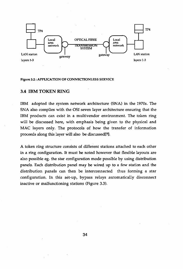
A token ring structure consists of different stations attached to each other in a ring configuration. It must be noted however that flexible layouts are also possible eg. the star configuration mode possible by using distribution panels. Each distribution panel may be wired up to a few station and the distribution panels can then be interconnected thus forming a star configuration. In this set-up, bypass relays automatically disconnect inactive or malfunctioning stations (Figure 3.3).

TP4

LAN station LAN station

r ai area network

34

I] DISTRIBUTION PANEL BYPASS RELAYS

- DISTRIBUTION I

PANEL

I

1 BYPASS RELAYS

A

STATIONS A,B,C,D,E,F

Figure 3.3 : STAR CONFIGURATION

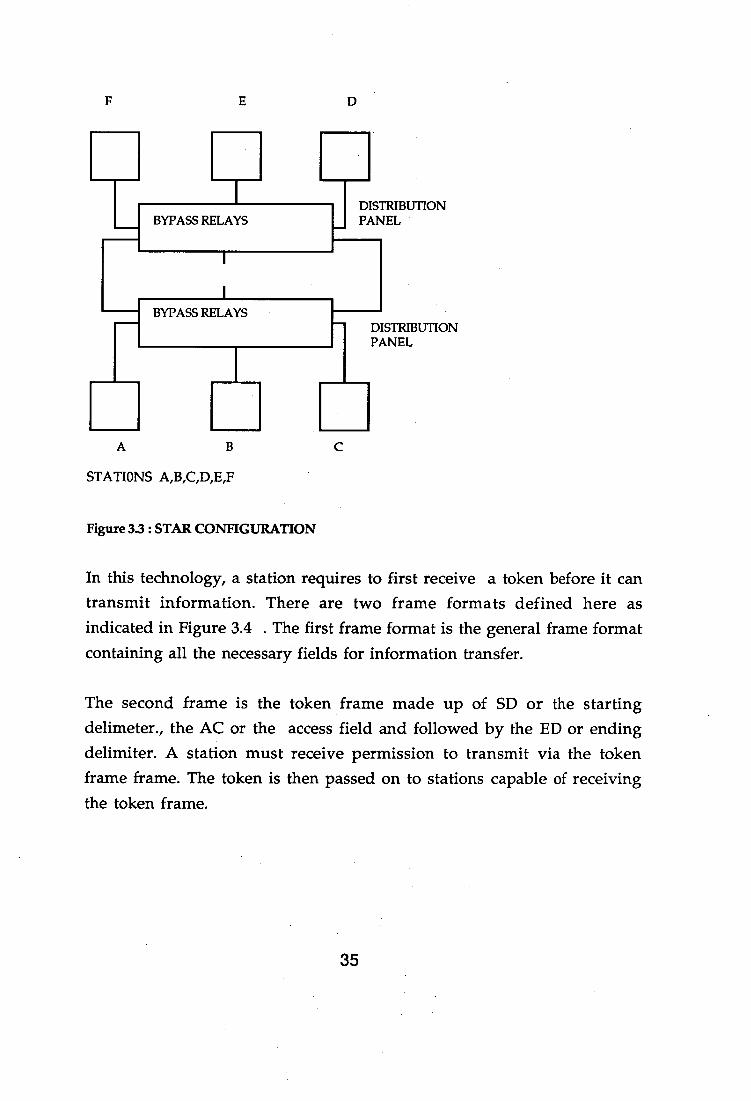
In this technology, a station requires to first receive a token before it can transmit information. There are two frame formats defined here as indicated in Figure 3.4 . The first frame format is the general frame format containing all the necessary fields for information transfer.

The second frame is the token frame made up of SD or the starting delimeter., the AC or the access field and followed by the ED or ending delimiter. A station must receive permission to transmit via the token frame frame. The token is then passed on to stations capable of receiving the token frame.

35

' SD I pc FC I DA SA I INFO I FCS ED FS

A. FRAME FORMAT

SD AC ED

B.TOKEN FORMAT

Figure 3.4 : POSSIBLE FRAME AND TOKEN FORMATS

A station can be typically in two different states. It can be in the transmit state where the station sends its own frame after receiving a token or it can be in a repeat state. In the repeat state, the station outputs the received frame bit by bit onto the ring. If the destination address of the frame is found to be its own, then it will copy the frame itself. It may modify some bits within the frame before transmitting it on the ring.

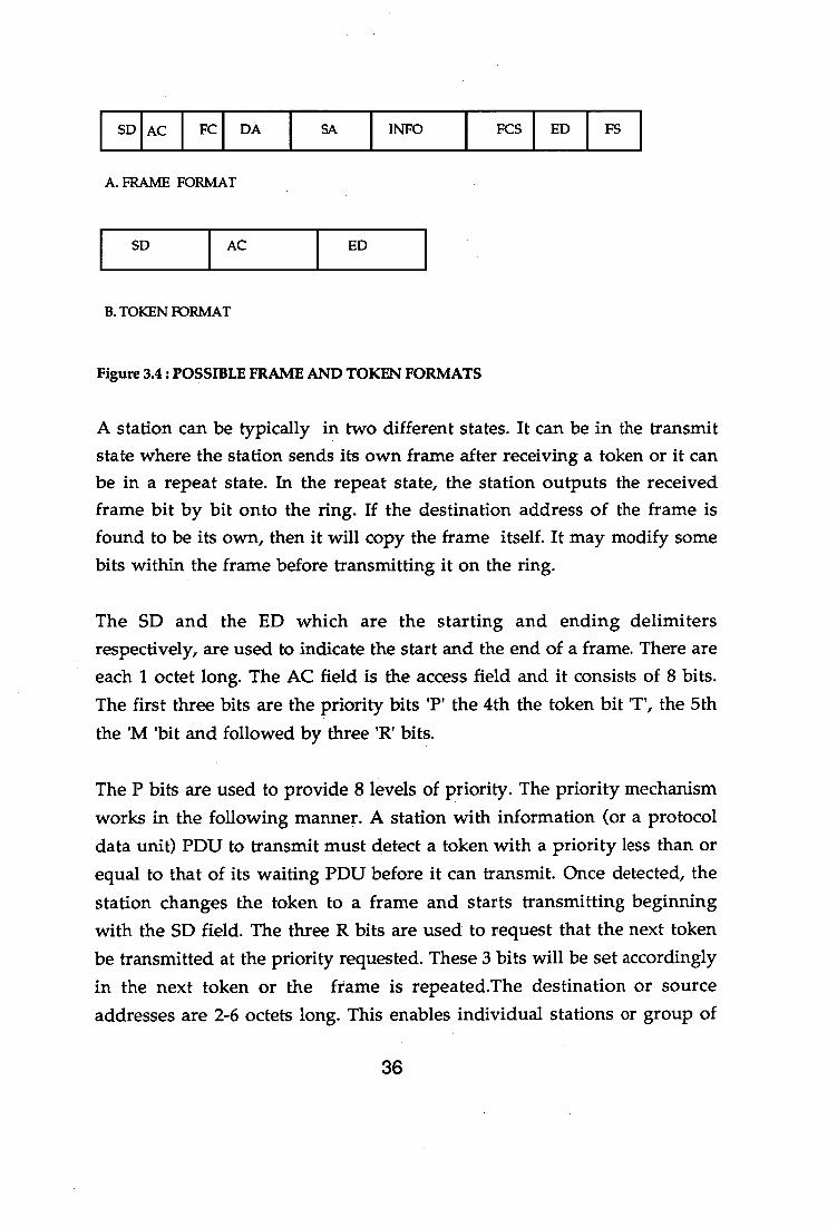
The SD and the ED which are the starting and ending delimiters respectively, are used to indicate the start and the end of a frame. There are each 1 octet long. The AC field is the access field and it consists of 8 bits. The first three bits are the priority bits 'P' the 4th the token bit 'T', the 5th the 'M 'bit and followed by three 'R' bits.

The P bits are used to provide 8 levels of priority. The priority mechanism works in the following manner. A station with information (or a protocol data unit) PDU to transmit must detect a token with a priority less than or equal to that of its waiting PDU before it can transmit. Once detected, the station changes the token to a frame and starts transmitting beginning with the SD field. The three R bits are used to request that the next token be transmitted at the priority requested. These 3 bits will be set accordingly in the next token or the frame is repeated.The destination or source addresses are 2-6 octets long. This enables individual stations or group of

36

stations to be addressed. A all 1 destination address is used to broadcast information to all stations on the ring. A frame check sequence, 4 byte cyclic redundancy check provides the bit error detection for the destination, source,routing information and information fields. The routing information field is only used when the frames leave the source ring and head for another new ring. All errors detected are then passed on the LLC or higher layers for correction.

The token is actively circulating a ring configuration. It may be possible for the token to be lost and this may occur when the ring is initialized or corruption occurs at one or more bits in the token itself. Alternatively, a fault in the SD can cause this problem. Another situation which can occur is a busy token may circulate indefinetly due to the T bit being set to 1 by noise. To recover from these problems, one station is designated to be an active monitor. It must be noted that each station has this capability of serving as a monitor and this provides a backup if one active station fails. The active monitor uses timers and the 'M' bit in the 'AC' field to recover from token or frame faults. On receiving a valid frame or token, the timer is reset. If the timer expires without a reset special purge frames transmitted continuously to signal all stations to switch to the repeat state and clear the ring of any distorted data. The active monitor then issues a new token. All frames , tokens have M bit in the AC field set to 0. If a token or frame reaches the monitor with the M bit set to 1 , this data is invalid and the active monitor purges the ring issuing a new token.

All aspects of the token ring access protocols are carried out at the medium access control sublayer. The functions of the physical layer is to receive bits one at a time from the MAC, encodes them and transmits them onto the medium. It also performs the reverse operation of taking symbols from the medium, decoding them and passing them to the MAC layer. The coding used here is the differential manchester coding. The typical bit rates of token ring can reach a maximum of 16Mbps and frame formats of sizes 15000 bytes are possible.

37

3.5 ETHERNET CSMA/CD

This is the second type of LAN which will be described here. The manufacturers of this kind of systems are the DEC or Digital Equipment Corporation. This group of vendors have also specified a group of standards similar to the OSI architecture referred to as the DNA or digital network architecture. This again enables a multivendor environment communication[7].

The CSMA/CD abbreviation simply means 'carrier sense multiple access/'collision detect'. This is the exact way in which the standards are defined. All stations listen for a carrier and if the carrier is absent they transmit messages. In this case there is a high probability of two or more stations transmitting at one time. When this happens, a collision is said to occur. The transmission must be aborted and all the information discarded. The re-transmission has to be scheduled again and it must be ensured that the second re-transmission time should be such that the probability of the same message getting through should be higher. The details of how the above mechanisms work will be explained in detail here.

38

receive • a a encoding

transmit data encoding

DATA LINK AYFR

transmit chn access

PHYSICAL LAYER

ETHERNET COAXIAL CABLE

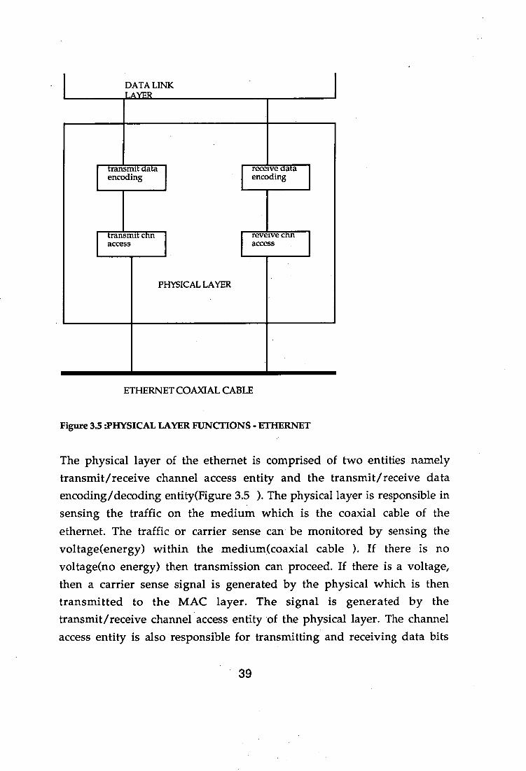
Figure 3.5 :PHYSICAL LAYER FUNCTIONS - ETHERNET

The physical layer of the ethernet is comprised of two entities namely transmit/receive channel access entity and the transmit/receive data encoding/decoding entity(Figure 3.5 ). The physical layer is responsible in sensing the traffic on the medium which is the coaxial cable of the ethernet. The traffic or carrier sense can be monitored by sensing the voltage(energy) within the medium(coaxial cable ). If there is no voltage(no energy) then transmission can proceed. If there is a voltage, then a carrier sense signal is generated by the physical which is then transmitted to the MAC layer. The signal is generated by the transmit/receive channel access entity of the physical layer. The channel access entity is also responsible for transmitting and receiving data bits

39

from the coaxial cable medium.The physical layer also monitors the voltage(energy) on the medium and compares it with the energy present in the originally generated signal. If there is a difference, this means more than one station is attempting to use the medium and the physical layer will generate a collision detect signal. The transmit channel access generates this signal and this is then transferred to the MAC layer.

The transmit/receive data encoding/decoding entity is responsible for encoding and decoding data as information moves up and from the higher layers respectively. The coding used here is referred to as the manchester coding.

40

LOGICAL LINK LAYER

transmit data receive data encapsulation decap ulation

transmit reveive link mangement

link management

MEDIUM ACCESS

CONTROL

Physical Layer

Figure 3.6 : MEDIUM ACCESS CONTROL- ETHERNET

The next layer is the MAC layer the format of which is given in Figure 3.6. The MAC layer utilizes the HDLC protocol where data is transferred over the LAN network is contained in a frame that includes, the address and error detection fields frame check sequence FCS, in addition to the data transmitted down from the higher layers. 12 octets are used for the source and destination addresses. 2 octets are reserved for use by the higher layers. A 4 octet or a 32bit frame check sequence is present at the end of each frame. The purpose of the error detection scheme is to detect any error present in the other fields present within a frame. If a error is detected, the error is then sent up to the LLC or higher layers for correction. The MAC

41

layer carries out the framing, addressing and error detection functions of the data link layer. To assist it, the MAC layer uses two entities. The first is the transmit/receive link management and the second transmit/receive data encapsulation/ decapsulation.

The transmit/receive link management entity manages the link watching out for the contention problems that arise and resolves them. Both the carrier sense signal and collision-detection signals are monitored by this entity. Once a collision is detected, a jam signal is issued and all stations abort transmission and wait for some time interval. Much of the contention resolution will depend upon how the time interval is selected. After much research, the binary backoff algorithm was found to yield the most satisfactory results. In essence, after the first collision the transmission is resumed after a time interval t. If there is a collision again, then the next transmission time is 2t and for each subsequent re-transmissions, the time interval is always double that of the previous value. Of course, there is a maximum value stipulated to prevent the degradation of performance of the ethernet. If any station retrys continuously and fails to transmit successfully within the maximum value stipulated, then transmission is aborted and the higher layers are informed of the failure of the message to be transmitted, This only happens if there is some serious fault fault within the configuration of the higher layers.

It is due to this mode of operation that there is a maximum value placed for the size of a frame. A frame cannot be too long as this would increase the collision rate within the ethernet. The maximum size of the frame is restricted to 1518 octets. This limitation ensures that the throughput and transmission delays are not adversely affected. Another important point is that the coaxial cable length of the ethernet should not exceed 1.5km to prevent degradation of signals. The typical bit rates of the ethernet can reach a maxim= of 10Mbps.

42

APPLICATION ASEs

FKESEN IA I ION-

bESSION

TKAN SFUK I

NETWORK

UN1 A

11-MICAL

I CAP

NULL

ISDN-UP

SCCF

Ml!' LEVEL 3

M11' LEVEL

Ml!' LEVEL 1

Chapter 4 :SS7 Signalling System

4.1 ARCHITECTURE

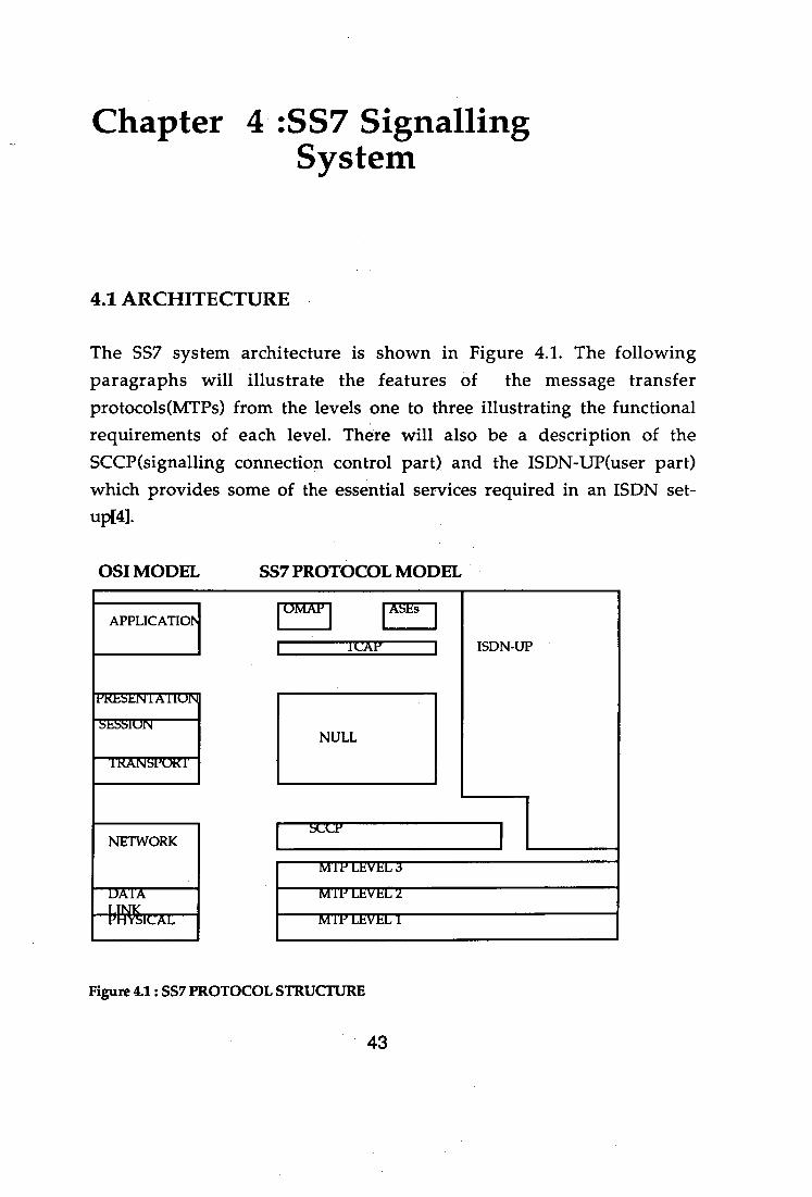
The SS7 system architecture is shown in Figure 4.1. The following paragraphs will illustrate the features of the message transfer protocols(MTPs) from the levels one to three illustrating the functional requirements of each level. There will also be a description of the SCCP(signalling connection control part) and the ISDN-UP(user part) which provides some of the essential services required in an ISDN set-up[tl].

OSI MODEL SS7 PROTOCOL MODEL

Figure 4.1 : SS7 PROTOCOL STRUCTURE

43

The MTP layers were designed much earlier than the SCCP or the ISDN-UP and these layers were primarily designed for the needs of telephony. Both the MTP layers and the SCCP form the NSP or the network service path. The NSF provides facilities to allow failures to occur without adversely affecting the transfer of information . The different protocols defined above correct the network failures thus enabling reliable transfer of information and service to be maintained. MTP comprises as mentioned previously of three levels which are as follows; the signalling data link functions, level 1 complying with the physical layer of OSI ; the signalling link functions, level 2 complying with the data link layer of OSI ; the signalling network function, level 3, complying with the network layer of OSI.

4.2 SIGNALLING DATA LINK FUNCTIONS (MTP LEVEL 1)

This refers to MTP layer or level 1 and this layer fully complies with the OSI physical layer. A signalling data link comprises of a bi-directional transmission path for signalling purposes consisting of two data channels operating together at the same data rate in opposite directions. A digital signalling data link comprises of transmission channels,terminal equipment TEs and a digital switch. The purpose of the digital switch is to provide an interface between the channels and the TEs thus providing for the facility to automatically reconfigure the transmission channels for the signalling links. The digital transmission channels comprise of a digital multiplex stream having frame structures as specified either for PCM equipment(telecom standards) or data(datacom standards). It is important to note that there are different representations for information transfer as specified either by telecom or by datacom standards. In the telecom standards, for voice the first bit(MSB) of an 8 bit octet format represents the sign bit. However, in data transfer (referring to datacom standards), the sign bit becomes the LSB. There is a complete reversal in bit representation.

44

The CCITT standard for the bit rates for the digital data link transmission is 64kbps. Analog data link transmissions are also possible however at a much slower bit rate which must exceed at least 4.8kbps.

4.3 SIGNALLING LINK FUNCTIONS (MTP level 2)

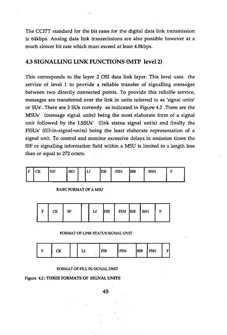
This corresponds to the layer 2 OSI data link layer. This level uses the service of level 1 to provide a reliable transfer of signalling messages between two directly connected points. To provide this reliable service, messages are transferred over the link in units referred to as 'signal units' or SUs'. There are 3 SUs currently as indicated in Figure 4.2 .There are the MSUs' (message signal units) being the most elaborate form of a signal unit followed by the LSSUs' (link status signal units) and finally the FISUs' (fill-in-signal-units) being the least elaborate representation of a signal unit. To control and monitor excessive delays in emission times the SIF or signalling information field within a MSU is limited to a length less than or equal to 272 octets.

F CK SIP SIO LI FIB FSN BIB BSN F

BASIC FORMAT OF A MSU

F CK SF LI FIB FSN BIB BSN F

FORMAT OF LINK STATUS SIGNAL UNIT

-

F CK LI FIB FSN BIB FSN F

FORMAT OF FILL IN SIGNAL UNIT

Figure 4.2 : THREE FORMATS OF SIGNAL UNITS

45

The SS7 link functions have strong similarities with the data network bit-oriented protocols(eg HDLC). Standard flags are used (flags 01111110) to open and close units. There is also a 16-bit error detection cyclic redundancy check. However, when there is no message traffic, FISUs are sent instead of flags(flags are sent in HDLC). There are other additional facilities provided here in comparison to HDLC to facilitate the network to respond quickly to system failures. The additional facilities provided are error correction, error monitoring and flow control mechanism each of which will be described here.

4.3.1 Error Correction (MTP 2)

The error correction procedures consist of two methods. The first is the basic method and the other is the preventive cyclic retransmission (PCR) method. All errors occurring in the MSUs' and LSSUs' are corrected while those in for the FISUs are only detected but not corrected. Another purpose of these methods is to avoid out of sequence and duplicated messages when error correction takes place. The PCR method is used when the propagation delays are large as in satellite transmission and in general is less efficient in the bandwidth utilization as compared to the basic method. Both methods will be described here.

4.3.2 The basic method

This is a non-compelled positive/negative acknowledgment retransmission error correction system. A positive acknowledgment from the receiver indicates to the transmitter that MSUs' were all received without any error. The transmitter can then discard all the buffered MSUs' which are copies of the previous signal units just after the last positive acknowledgment. If there is a negative acknowledgment sent to the transmitter, the transmitter will roll back and resume retransmission of the previously outstanding messages beginning from the last positive acknowledgment point. Again the transmitter waits for the positive

46

acknowledgment before discarding the MSUs. For sequence control,each signal unit is assigned a forward and backward sequence numbers and indicator bits. The sequence numbers are 7 bits long ('FSN', 'BSN') and a maximum of 127 messages can be transmitted before the first positive

acknowledgment is issued by the receiver to the transmitter.

4.3.3 PCR method

This is a non-compelled positive acknowledgment cyclic retransmission forward-error correction method. In this method, only the positive acknowledgments are sent by the receiver to indicate correct MSU arrivals. The transmitter in the event of having no new MSUs , retransmits cyclically all the messages which have not yet been acknowledged. A threshold value is ascertained to indicate what is the maximum allowable MSUs to remain unacknowledged at any one time. If this value is exceeded, there is a strong indication that error correction is not being done. This situation may be aggravated by a high level of new incoming MSUs waiting to be transmitted. In this case, once the threshold value is exceeded, the system goes into a forced retransmission mode to retransmit the outstanding messages which have not yet been acknowledged . This continues until the transmitter gets a positive acknowledgment for these messages thus ensuring that the outstanding messages fall below the threshold value. The network designer must be careful in setting the threshold value, as a low Value will cause the link to cycle in and out of the forced retransmission mode.

4.3.4 Error monitoring

There are two types of signalling error rate monitoring procedures described here. The first is the signal unit error rate monitor used while a service link is operational. It provides the criteria to decide when a link should be taken out of service due to excessive error rates. The second procedure is the alignment error rate monitor used while the link is in the proving state or initial alignment and this provides the criteria to accept or

47

reject a link during the initial alignment stage due to excessive errors. Both these mechanism provide an effective measurement of how efficient and reliable a signalling is, thus ensuring that the transmission rate of the SUs' from the lower layers (physical,data link layers) to the higher layers(network and higher layers) does not deteriorate over a period of time. Faulty links can be located by their high error monitor recordings and can be replaced to ensure maximum throughput.

4.3.5 Flow control

This is another mechanism present in the signalling link functions to prevent an excessive build up of signalling units. As the traffic level increases to the point where there is congestion, the receiving end notifies the transmitting end of its congestion problem with an LSSU(indicating a busy status) and withholds acknowledgment of all incoming signal units. This prevents the link transmitting end from failing a link due to excessive outstanding messages. However, if this condition perpetuates for a period between 3 to 6 s, the transmitting end will fail the link.

When there is an indication that level 3 has failed and level 2 recognizes or is notified of this failure, then level 2 sends a 'signalling indication processor outage' (SIPO) to the far end indicating that signalling messages cannot be transferred to level 3 or higher layers. The far end, having its own MTP layers, will send a FISU from its own level 2 to level 3 informing its own MTP layers of the SIPO condition. The far end level 3 will re-route the outstanding traffic according to the network management procedure.

4.4 SIGNALLING NETWORK FUNCTIONS (LEVEL 3)

This corresponds to the lower half of OSI's network layer and provides functions and procedures for the transfer of information between signalling points which are nodes of the signalling network. The network

48

function can be divided into two procedures, the first being the message handling procedure and the other the network management procedure.

4.4.1 Signalling message handling

This procedure functions include message routing,discrimination and distribution functions. These functions are provided at every signalling point within the signalling network. To do this , the MSU is utilized. A 'routing label' is placed at the beginning of a 'SIF' and both the routing label and SIO(service information octet) within a MSU are utilized to handle the messages. The routing table consists of DPC, OPC and a SLS code. DPC stands for to the destination point code while the OPC refers to the originating point code. The SLS stands for to the load sharing link code usually utilized to evenly spread the utilization of all available links.

When a message comes from level 3 user, or originates at level 3, the choice of which signalling link is to use is made by the message routing function. When a message is received from level 2, the discrimination function is activated and this determines if the message is addressed to itself or to another signal point. The DPC is checked and the message routing is based on the SLS codes ensuring that any one particular link is not overloaded thus causing an imbalance in the network. The SIO is also required to provide additional information to further enhance the routing scheme adopted.

4.4.2 Signalling network management

This management function is responsible for the reconfiguration of the signalling network to control the traffic flow. In the case of congestion or blockages that may arise. The important objective here is that when failure occurs, the reconfiguration is carried out so that messages are not lost or duplicated. Within this signalling network management, three functions are defined. They are the signalling traffic,route and link management

49

procedures. When there is a change in the status of a signalling link , route or point, all these procedures are activated. These are the procedures referred to in the flow control section and a brief description of each will be given here.

The signalling traffic management procedure is responsible for diverting traffic from signalling points without the loss or duplication of messages. This function routes traffic to various available alternatives. When routes become unavailable or available , forced re-routing and controlled re-routing techniques are used respectively to divert traffic to alternative routes or to the routes made available. Controlled re-routing is used to divert the message route to an alternative more efficient path.

Another procedure, the signal route management is used to distribute information about a network to block or unblock routes. Routes may have to be blocked if they are over utilized and experience congestion. Signalling transfer points (STP) and DLCs' are used to assist in the execution of this function.

The last procedure, is the signalling link management procedure. This is used to restore failed signalling links, to activate new signalling links and to deactivate aligned signalling links. The last point refers to the process of alignment proving procedure that each link has to go through before being approved and put into service state. It may become necessary to deactivate such a link due to the high error rates occurring during service time. This concludes the description of the first MTP 3 level functions.

43 SIGNALLING CONNECTION CONTROL PART(SCCP)

The first three MTP layers were designed primarily for the telephone system. The SCCP, which forms the upper layers of the SS7, was specially designed to provide additional addressing capability to the MTPs for the ISDN set up. This design justifies the additional overhead incorporated in

50

the SCCP which is not present in the first three MTP layers.

The SCCP supplements the MTP layers addressing capabilities and uses the DPC plus sub-system numbers(SSNs) which are local to the SCCP users at a particular node. The SCCP provides four classes of service, 2 connection oriented and 2 connectionless to further the addressing capability of this layer.

The SCCP can be divided into 4 functional blocks. The first being the connection oriented control block. This block provides control establishment and release of a signalling connection followed by data transfer. The second is the connectionless block which caters for the connectionless transfer of data. This is followed by the management block which provides the capability beyond those of the MTP levels to handle congestion or failure at either the SCCP user or the signalling route to the SCCP user. This enables the SCCP to route messages to back up the system in the event that failures prevent routing to the primary system. The last block is the SCCP routing block and its functions as follows. This block takes received messages from MTPs or other functional blocks and performs the necessary routing functions. This concludes the 4 functional block descriptions of the SCCP.

4.6 ISDN-UP

This layer will be the final element of the SS7 discussed in this report. The ISDN-UP(user part) has some of the most essential features needed in the ISDN technology. The ISDN-UP can provide the basic bearer service and the supplementary services which enhance the operational functions of the previous layers or levels discussed earlier. The ISDN-UP messages identify the originating and destination addresses, provide circuit identification codes (CIC) and a message code that uniquely define the function and format of each ISDN-UP message.

51

The basic bearer service provided in ISDN-UP is essential for the control of circuit network connections between the subscriber line and the exchange termination. It also sets up the trunk connections, call and release connections for the circuit switched network.

The supplementary services provided include a user-to-user signalling service, a closed-user group service, call line identification and forwarding services. The user-to-user signalling service provides communication to end users through the signalling network for the purpose of exchange of information of end-to-end significance. The closed - user group service enables communication to proceed within a fixed small group of people with the option of having incoming and outgoing access to users outside this group. The call-line identification enables the caller's number to be displayed at the called party's location. Finally the call forwarding facility provides a user to re-direct incoming calls to another number. This summarizes the services offered by the SS7 signalling network.

52

Chapter 5 : ISDN PABX & LAN INTEGRATION

5.1 THE PABX

.In a typical office environment, there may be about 100 telephone users within the office environment. In terms of management and cost, it will be highly inefficient to link up each of these 100 lines directly to the public switched telephone exchange(PSTN) leading to the exchanges. Instead, the common practice is to have all the 100 extensions attach themselves to a private exchange which then can be linked up to the PSTN. An automatic private exchange is referred to as a PABX.

In principle, the PABX for a typical office environment today, must be able to handle voice and also information transfer equipment. In the early 1960's much of the design for the switching facilities within the PBX depended on mechanical devices relays and operators manually performing the switching of the lines. However, with the widespread of the micro-chip revolution in 1970's, the new PBXs' were designed more elegantly and were automatic. Currently, in the 1990's, most PABX designs are catering more for the integration of all digital services in the near future. Thus all modern PABX designs cater for both voice and data transfer facilities simultaneously.

Referring to the ISDN terminologies, the modern PABX contains the functions of both the network termination 1(NT1) and network termination 2 (NT2). In this following section, there will be a description of the requirements of a modern PABX and this will be followed by ways in which the modern PABX can be upgraded to an ISDN PABX.

53

5.2 THE MODERN PABX

The design described here gives a modern system which will cater for the conventional telephone system, digital telephones and for also data transmission. Transmission for the conventional telephones is done using the decadic or DTMT signalling(according to CCITT recommendations and will proceed via analog trunk circuits to the public exchange(PSTN) leading to the circuit switching networks. The transmission for digital telephones or data can use the digital trunk circuits and proceed to the packet switching networks. All relevant information which will follow for the subsequently for the PABX design has been taken from the Erricsson Design Manual.(MD110 Digital PABX reference book)[6].

Figure 5.1 is a typical example of a modern PABX. All attachments are made to the line interface module ,the LIM. The set up indicated can have a capacity of up to 200 extensions within an environment. All of the functions illustrated in the Figure 5.1 will be explained.

54

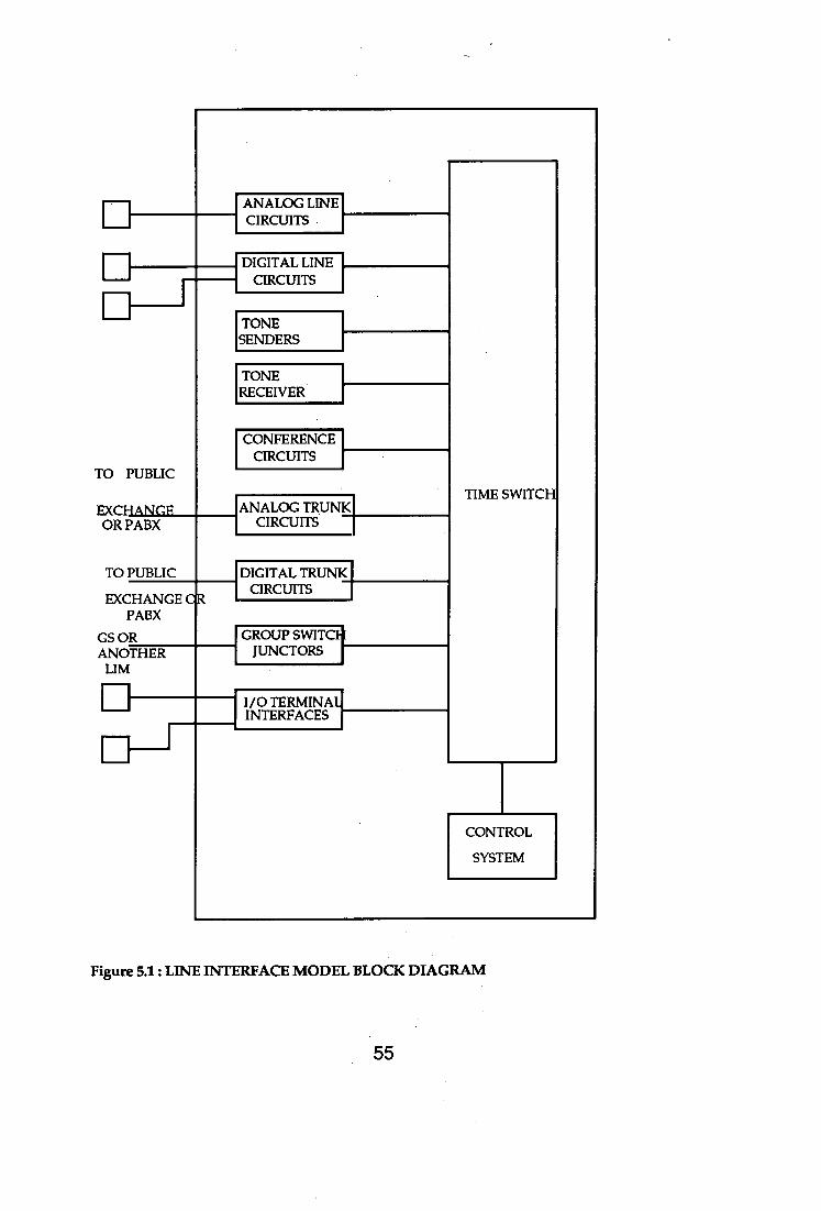
ANALOG LINE CIRCUITS

DIGITAL LINE CIRCUITS

TO PUBLIC

EXCH A NCT. OR PABX

TO PUBLIC

EXCHANGE CR PABX

GS OR ANOTHER

UM

TONE SENDERS

TONE RECEIVER

CONFERENCE CIRCUITS

ANALOG TRUNK CIRCUITS

DIGITAL TRUNK CIRCUITS

GROUP SWITCH JUNCTORS

I/O TERMINAL INTERFACES

TIME SWITCH

CONTROL

SYSTEM

Figure 5.1 : LINE INTERFACE MODEL BLOCK DIAGRAM

55

The 'analog line circuits' box indicated caters for the connection of conventional telephones using decadic or DTMF signalling. Analog signals are converted to digital signals within the analog line circuits to enable time switch (TS) and the control system(CS) to process the information. At the 'analog trunk circuits' interface, signals are converted back to analog form and are sent to the public switching telephone network. or alternatively it could be connected to another PABX via 'analog trunk circuits' interface thus extending the capacity of the PABX. The analog/digital conversions takes place by the use of single channel codecs.

The 'digital line circuits' are used for connection of operator consoles and digital telephones via normal two wire twisted pair lines. The 'digital trunk circuit' receives all the information from the digital systems connected to the 'digital line circuits' and then transmits the information to other digital exchanges. A 'digital trunk circuit' corresponds to 30 conventional 'analog trunk circuits'.

The 'tone senders' and 'tone receivers' are devices for the generation and reception of tones(eg dial tone,busy tone) both for the conventional DTMF signalling telephones and for the digital system telephones. A tone sender unit 'TSU' supplies the LIM (line interface module) will all tones. The 'TRU' or tone receiver units contain receivers for the conventional DTMF telephones and also for digital telephones.

The 'MPU' or the multiparty conference unit is used to achieve a flexible number of conferences with 3-8 users simultaneously and this function provides additional communication facilities within the PABX environment.

The 'control system' (CS) is the heart of the line interface module. It consists of a LIM processor unit (LPU) comprising of two commercial 8 bit microprocessors. The first microprocessor functions as the LIM's main

56

processor while the second processor works as a signal processor and handles direct communication with the control circuits of the time switch and the telephony devices. The control system also has a number of MEU or memory boards which store the LIM programs and data. Each MEU contains RAM type storage components having a capacity of 256kbytes.

The 'time switch' consists of one basic board, the BSU (basic switch unit) and two supplementary boards (SSUs). The function of the BSU is to contain the voice and control memories for the time switch as well as a microprocessor. It controls the internal functions of the switch and has contact with the second microprocessor in the LPU(i.e the signal processor) The two SSU boards have 256 timeslots each and undertake serial/parallel conversion of the PCM signals to and from the device boards.

The 'group switch junctor' board is usually connected up to two 32 channel timeslots PCM links. These links are connected up to group switch to expand the capacity of the system. Timeslots in the PCM link are numbered starting from 0-31 and timeslot 0 is reserved for synchronization while timeslot 16 is used for control of signals involving the D channel. Thus 30 channels are available for voice or data transmission. Each LIM has two group switch junctors and since one group junctor utilizes 2 PCM links , 2 group junctors will utilize 4 PCM links. By the use of a group switch, it is possible to link up more than one LIM and extend the capacity of link extensions beyond the 200 limit.

The I/O interface boards are used for operation and maintenance functions. Up to six terminals can be use concurrently for fault locating, operational maintenance for additional installation of software or programming which may be required to enhance the performance of the line interface module(LIM).

The LIM(PABX) described also uses SS7 signalling system the details of which will be described shortly. This form of signalling is a pre-requisite

57

for the ISDN standards as described in the Q series. However, the PABX must be modified to support the ISDN technology. The details of the modifications will be discussed now.

5.3 ISDN PABX

The previous chapter has indicated what are some of the essential features within a common signalling system like the SS7. A PABX must support the SS7 signalling before it can be upgraded to a integrated or ISDN PABX. Another similar system, the DPNSS which is in widespread use in the United Kingdom(UK) can also support the ISDN signalling functions. In fact, this system which was developed by British Telecom and is currently in widespread use in PABXs' designs. This is because the DPNSS was specially designed for use in the PABX systems while the SS7 system was aimed at public exchange networks. However, as the ISDN standards become more clearly specified in 1990's , it becomes advantages for all designs to migrate to the SS7 signalling system thus ensuring a common standard is adopted and maintained amongst all vendors in the communication industry . The PABX design described in the earlier part, the Erricssons design, supports the SS7 signalling system.

Another essential component of an ISDN PABX is that each extension within the PABX system must support '2B + D' channels. The bit rates at the S interface must be large enough to support a '2B + D' channel system.

To gain access to the bit rates, a IVDM or integrated voice data module can be used and a data terminal and a telephone set can then be attached to it. The IVDM intum is connected up to the PABX and the interface between the IVDM and PABX can then be referred to as the S interface. This enables that the existing facilities to be linked up to a single module which will effectively integrate both voice and data transmission.

Another solution for the kind of equipment used, is to use a IVDT or

58

integrated voice data terminal. This is a more elaborate solution as both voice and data facilities can be obtained from one terminal. A terminal communication board (TCB) can be designed and fitted into a terminal converting it into a integrated voice data terminal. (IVDT)

If the primary rate access is used at the 'S and 'U' interface of the integrated PABX design , then each B channel at the S interface will require 64kbps and the two B channels will require 128kbps. The D channel for the primary rate access is 64kbps and this is required for signalling purposes.

5.4 INTEGRATION OF ISDN PABX & LAN

This part of the report will examine what are some of the critical issues involved in a a ISDN PABX/LAN system and also suggest one such design. Much of the discussion will be based on the already existing ISDN and LAN standards as the new standards for this scheme, the IEEE 802.6 are not available at this time[8].

The typical high speed data which belongs to a LAN is unsuitable in a circuit switched transmission environment. High speed packet data is bursty in nature. Although circuit switched networks can be used to transmit several mega bits of data, it does not ensure a efficient mode of transmission for high speed bursty packet data. Therefore LANs have been used handle this kind of high speed data using packet switched networks. PABXs have been used to handle both voice and packet data (9.6kbps-48kbps)

An integration of the ISDN PABX and the LAN can suggest two possible layouts. The first is to attempt to integrate voice within a LAN system. This solution is not feasible due to the high frequencies required for voice transmission. The sampling frequencies for voice is 80001 -1z as previously

mentioned to enable digitizing of the voice samples by the PCM technique. Data on the other hand, does not require such high frequencies , especially

59

high speed data since the product of the bits and the frequency is equal to the bit rate. For high speed data, the bits within a frame are higher than that for the low speed data and for a fixed bit rate, low frequencies are sufficient for transmission.

The alternative solution is to integrate a LAN within a PABX environment. In this way voice samples can be sampled at 8KHz and data at lower rates . The ISDN PABX does not have to support interfaces for the high speed packet traffic to move between one PABX to another or even to PSTN. The LAN traffic is local and only known within the PABX environment. Separate facilities are required for processing the high speed packet information.

The implementation must also ensure that existing transmission media(eg twisted pair) can be utilized for transmission purposes. This will ensure efficient usage of existing facilities within the new proposed design thus saving costs. IVDM or integrated voice data modules can be used and terminals or equipment for the high speed data, normal speed packet data(48kpbs X.25) and voice facilities can then be attached to it thus creating a integrated services environment for the '2B + D + P' channel interface. The 'P' channel interface refers to the channel which supports the high speed LAN packet data. Alternatively, IVDT or integrated voice and data terminals can be used to support the '2B +D + P interface provided the terminals bit rates are high enough to support the different services,

The medium access control procedures for both ethernet and token ring were previously discussed earlier, according to their standards. The ethernet can have a maximum frame size for 1500 bytes for information while token ring environment can have frame sizes exceeding 15000bytes. A standard must be fixed to ensure that the frame sizes in this implementation are not too long as the delays for transmission would increase.

60

A delay in transmission time will result in a smaller number of frames being transmitted per second In image processing, even at very high bit rates (1.536Mbps), transmission delays must be controlled to ensure that the right kind of images are produced. For example, if the transmission delay is 1s at a bit rate of 1.536Mpbs , then this mode of transmission will be unsuitable for computer graphics as only still images will be produced. A transmission time of 0.4seconds on the other hand will produce 2,5frames/s and will be ideal for computer graphics or other image processing applications.

61

Chapter 6 : PROPOSED DESIGN

6.1 DESIGN CONSIDERATIONS

The following implementation which will be described here is one of the possible solutions for the integration of both the ISDN PABX and a LAN system. The design is taken from [8[ and a detailed explanation of the set-up will be given here.

To connect a '2B+D' interface to a PABX, the PABX requires a SPM or speech path module. Referring to the PABX design described earlier, this is implemented in the form of digital line circuits. These digital circuits are then connected to a switching system which is also linked to a microprocessor. With the aid of both the switching system and microprocessor, information will be routed in the PABX to the required destination.

In order to extend this capacity to incorporate the high speed data channel i.e. the 'P' channel, the new interface which has to now be dealt with is a '2B + D + P' channel interface. While the '2B + D' channels are handled by the PABX, a BSM or burst switching module is required to handle the P channel(or the high speed data channel)[81.

6.1.1 Terminal communication board

The terminals used here are the IVDT or integrated voice and data channels . Each such terminal has a bit rate of 2.048Mbps. For the '2B + D + P' channels interface, the P channel requires 1.536Mbps. The remaining 0.512Mbps is used for the '2B + D' channels and also for other purposes including frame synchronization and maintanence.. To implement such a architecture, the terminal communication board must be designed as

62

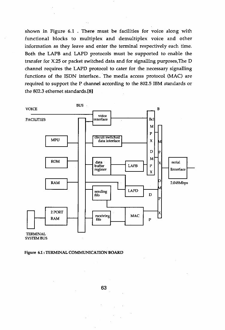
serial

linterface

2.048Mbps

Bct FACILITIES voice

interface

MPU

ROM

RAM

circuit switched data interface

—1 data buffer register

X

X LAPB

—1 sending fife

LAPD 11:0

2 PORT

RAM _I receiving fifo

MAC

TERMINAL SYSTEM BUS

shown in Figure 6.1 . There must be facilities for voice along with functional blocks to multiplex and demultiplex voice and other information as they leave and enter the terminal respectively each time. Both the LAPB and LAPD protocols must be supported to enable the transfer for X.25 or packet switched data and for signalling purposes,The D channel requires the LAPD protocol to cater for the necessary signalling functions of the ISDN interface.. The media access protocol (MAC) are required to support the P channel according to the 802.5 IBM standards or the 802.3 ethernet standards.[8]

BUS VOICE

Figure 6.1 : TERMINAL COMMUNICATION BOARD

63

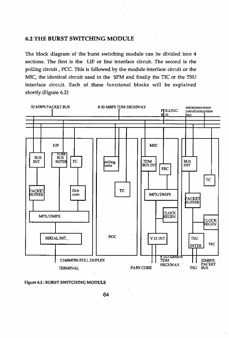
32 MBPS PACKET BUS

LIF

1UM BUS

BUS INT

INTER

8-32-MBPS TDM HIGHWAY LLING

BITS

microporcessor communicastion bus

MIC

Dolling :ontr

TDM BUS INT

BUS INT

TC

6.2 THE BURST SWITCHING MODULE

The block diagram of the burst switching module can be divided into 4 sections. The first is the LIF or line interface circuit. The second is the polling circuit , PCC. This is followed by the module interface circuit or the MIC, the identical circuit used in the SPM and finally the TIC or the TSU interface circuit. Each of these functional blocks will be explained shortly.(Figure 6.2)

FEC

TC

?ACICET Dch

TC BUFFER cont MPX/DMPX

PACKET BUFFER

LOCK MPX/DMPX _12EGEN

CLOCK tECEN

SERIAL INT.. PCC V.11 INT

TSU

INTER TIC

8 1U 32MBPS 2.048MPBS FULL DUPLEX

TDM 32MBPS HIGHWAY PACKET

TERMINAL PABX CORE

TSU BUS

Figure 6.2 : BURST SWITCHING MODULE

64

6.2.1 LINE INTERFACE CIRCUIT(LIF)

All terminals gain access to the facilities of the BSM via the LIP. As the bit rates of 2.04Mpbs arrive at the LIP, the '2B + D' channels are demultiplexed in the LIF. The 'P channel is also demultiplexed and information is passed through a packet buffer which is used because of the difference in the access line speed (1.536Mpbs) and the packet bus (32Mpbs). The LIF is linked up to 4 different lines or bus connections. The first is the 32Mpbs packet bus which is used for the transfer of high speed packet data. This is a 8-to-32Mpbs TDM highway is used for the transportation of the '2B' channels to and from speech path module or the MIC. The third is the polling bus. Here, all terminals have to poll become the are allowed to send information to the BSM. The polling bus via the polling controller, handles information as to which terminal gets to transmit information on the 32Mbps packet bus next. The fourth bus is the microprocessor communication bus. The D channel is demultiplexed and is passed over to a D channel controller. The terminal controller is present because here, each terminal controller has to co-ordinate polling via the polling controller. In the LIF, the terminal controller also transfers the D channel signalling information via the microprocessor communication bus to the speech path module or the MIC (SPM)[8].

6.2.2 POLLING CONTROL CIRCUIT (PCC)

The function of the polling control circuit is to co-ordinate different terminals to gain access to the 'P' channel facilities within the BSM. This controller selects on terminal out of the different terminals polling to use the BSM. The selected terminal can then use the 32Mbps packet bus. The polling time delay for one terminal is given as 1.6*10 -6s. This small time delay ensures that a large number of terminals can be linked up to the BSM simultaneously[8].

65

6.2.3 MODULE INTERFACE CIRCUIT(MIC)

This part of the BSM represents the speech path module within a PABX. This circuit contains digital line circuits as mentioned in the Erricssons PABX design which was described earlier. The purpose of these circuits is to multiplex the incoming '2B + D' channels onto a TDM time division multiplexed highway of speeds between 8-to-32Mpbs. These high speeds are required so as to ensure that many '2B + D' channels having a bit rate of at least 192kpbs can use the highway simultaneously. this highway is then linked up to a switching network. The switching system is similar to the 'time switch' which was described in the PABX design. The switching network is linked up to a central processor. The central processor is equivalent to the 'control system' described in the PABX design.Thus a BSM can be directly linked to the PABX core without modifying any of the PABX design[8].

Before explaining the final component of the BSM, the TIC or the TSU interface, it is first important how the high speed data can travel within the BSM. There are two kinds of traffic that can be possible. The first is the packet traffic which is local to a BSM. A BSM can support up to 100LIF cards. Each card can support 4 terminals. A BSM can therefore support 400 terminals. If the traffic is local, then information transfer can only take place within the 400 terminals. The second type of traffic is the inter BSM traffic. The traffic here is between BSMs only. Packets travel between a BSM via a TSU or Tandem Switching Unit utilized for the purpose of extending the system capacity beyond the 400 terminals mark. A TSU can be used to support up to a maximum of 8 BSMs at one time.

6.2.4 TANDEM SWITCHING UNIT INTERFACE CIRCUIT(TIC)

The TIC, the final part of the BSM is used to support packet traffic between different BSMs by using the facilities of a TSU which will be described shortly. The TIC has a TC terminal controller and a packet buffer. The

66

terminal controller, as previously explained is required for assisting in the polling of the terminals. The packet buffer is required for coordination and adjusting for the imbalance in speeds of the packet data. due to polling. The TIC is then connected up to a TSU or tandem switch unit via a 32Mpbs packet bus. This completes the description of all the various components within a BSM

The next stage of this discussion is to examine the functions of the the high speed packet tandem switching unit, the TSU. The TSU can be connected up to the BSMs and this way more than one BSM can be used in this set up. The TSU can then be linked up to the central processor (or a control system as in the earlier PABX design). If the control system is implemented as in the Ericcsons design, more powerful microprocessors may have to be used since there is a greater load on the PABX system[8].

6.3 TANDEM SWITCHING UNIT(TSU)

The TSU is a matrix self-routing switch. It utilizes 4 sets of 4x4 switches to perform its functions. There are 8 input ports entering the TSUs from the BSMs and 8 output ports on the other end of the TSU (Figure 6.3).

67

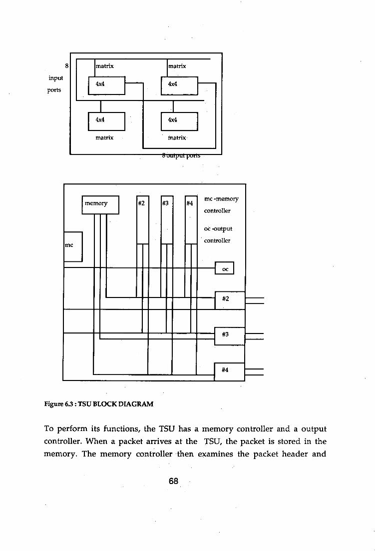
MC

mc -memory

controller

oc -output

controller

I #2

#3

#4

memory #2 #3 #4

input

ports

8

Figure 6.3 : TSU BLOCK DIAGRAM

To perform its functions, the TSU has a memory controller and a output controller. When a packet arrives at the TSU, the packet is stored in the memory. The memory controller then examines the packet header and

68

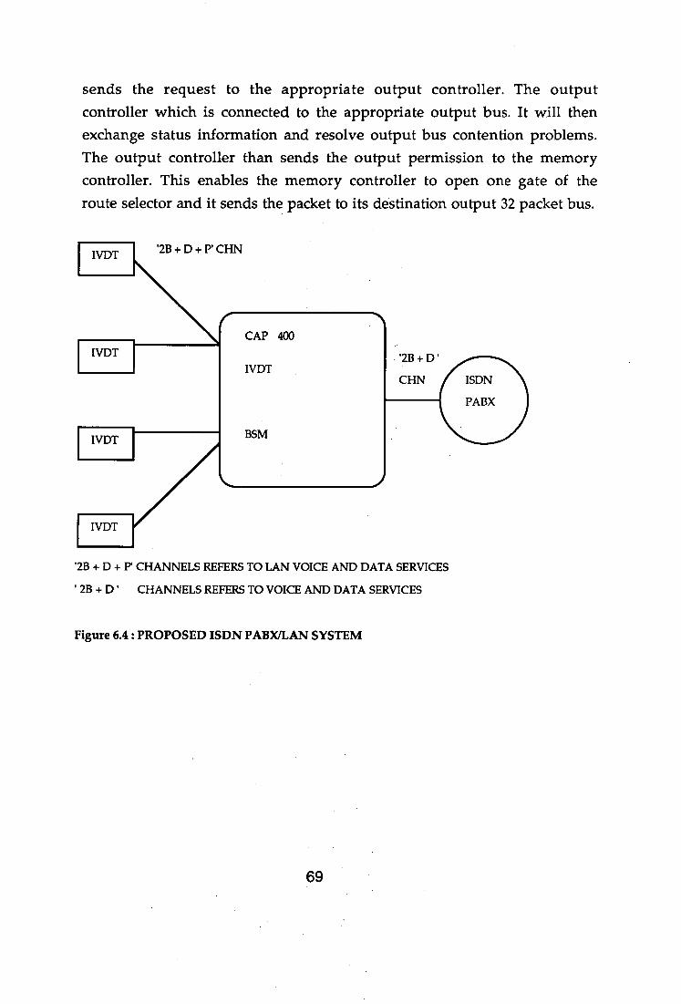
CAP 400

IVDT

IVDT

BSM

IVDT

IVDT

sends the request to the appropriate output controller. The output controller which is connected to the appropriate output bus. It will then exchange status information and resolve output bus contention problems. The output controller than sends the output permission to the memory controller. This enables the memory controller to open one gate of the route selector and it sends the packet to its destination output 32 packet bus.

IVDT '2B + D + P CHN

'2B+D'

CHN ISDN

PABX

'2B + D + P' CHANNELS REFERS TO LAN VOICE AND DATA SERVICES

' 2B + D ' CHANNELS REFERS TO VOICE AND DATA SERVICES

Figure 6.4 : PROPOSED ISDN PABX/LAN SYSTEM

69

BSM (BURST SWITCHING MODULE)

TSU

(TANDEM SWITCHING

UNIT)

Figure 6.5 : A MAXIMUM OF 8 BSMS' CAN BE CONNECTED TO A TSU

70

Chapter 7: PERFORMANCE SIMULATION AND RESULTS

7.1 SIMULATION PROGRAMS

Having described the functional operations of the BSM and the TSU, it now becomes necessary to study the performance of both systems and examine the delays. The simulation of both systems was done using Simscript version 2.5.

7.1.1 Design for BSM

Let us consider the different steps involved in designing a suitable simulation program for the performance of thel BSM. In this section, the packet information transfer only local to a BSM will be considered. The inter BSM traffic will be dealt in the performance evaluation of the TSU.

Referring back to the BSM functional blocks(Figure 6.2), it can be noted that for local traffic within the BSM , all blocks excluding the TIC will be used. For the high speed packet data, the LIF and the PCC will both be utilized while the MIC will be used for the '2B + D' channels. High speed data leaves the IVDT terminal and gets onto the access line which has a speed of 1.536Mpbs. The bit rates of the IVDT terminal is 2.048Mpbs. The remaining 0.512Mpbs is used for the '2B + D' channels, frame synchronization and maintenance. The demultiplexed '2B + D' channels are then passed onto the MIC or speech path module.

If the size of the packet or message is 'K' bytes, then the time taken for the packet to reach the packet buffer is (K*8)/1.536M) s. There is also a polling

71

delay and the polling delay for each terminal is given in [8] as 1.6 440-6 . If there are i number of terminals attached to the BSM, then the total polling

time will be (i*1.6*10-6)s. The third delay component present here is the average waiting delay within the BSM due to the utilization of the 32Mpbs packet bus. The average waiting time of a packet within the BSM will depend on the utilization of the packet bus.The higher the utilization, the higher the waiting time. However, it is suggested that the delays can be kept at between 2-3 ms if the bus utilization is below 80%.

Another concern is the interarrival times of the packets or messages. The packet interarrival times can follow different distributions available in the 'traffic theory'. However, it has been stipulated that the arrival follows a Poisson distribution. Equivalently , a negative exponential distribution will be used for the interarrival times.

The high speed packet data has a packet size which is exponentially distributed with a mean of lkbyte. The line access speed is 1.536M. This means that access line takes a delay of (8/1536) = 0.005208s to send the message to the packet buffer.The mean frequency of the packet can also be calculated and it is (1/0.005208) = 192Hz. As expected, the frequency for the packet is much lower than that for voice.

The following points will summarize the various components involved in the design of the performance model.

Component 1. Interarrival time : t ; exponentially dist.

2. Polling time per terminal: 1.6*10 -6s ;constant

3. Message time : 0.0052ms ; exponentially dist.

4. Service time BSM : case 1 : 3ms ; exponentially dist. case 2 3ms ; constant.

5. Number of Jobs : J ; 500, 1000

72

Component number five allocates one job to each terminal. A BSM can serve up to 400 terminals. Increasing the number of jobs does increase the total delay the results of which will be referred to later.

To explain component number 4, the mechanism of the transfer of high speed data must be understood. There can be a maximum of 4 terminals attached to one LIF cards. A BSM can take up to a maximum of 100LIF cards. All terminals connected to the BSM poll for the use of the 32Mpbs packet bus.. The PCC decides and selects one terminal. The information as previously explained enters the LIF and gets onto the access line marked 'P' in the LIE layout. The access line operates at 1.536Mpbs while the 32Mpbs packet bus operates about 20 times faster.(32/1.536 = 20). If the packet bus utilization is low, the packets which arrive through the access line will immediately get onto the 32Mpbs packet bus. However, when the packet bus utilization gets higher, packets will begin to queue in the packet buffer.

Two cases are examined here. The first case is when 100% of the 32Mpbs packet bus is used with service times exponentially distributed (mean 3ms). The packet bus in this case is 20 times faster than the access line. In the second case,only 80% of the 32Mpbs packet bus capacity is used and the service time is a constant (3ms). The utilization of the packet bus is only 80% which means the packet bus is only 20*0.8 = 16 times faster than the access line. The two cases are simulated for the different interarrival times and number of jobs.

It becomes possible to highlight all the delays involved here.

Delay Component 1. Polling time 2. Message time 3. Service time 4. Message time

73

The fourth delay element refers to delay generated when the destination terminal picks up the packet data addressed to it via the LIF. The packet information is transferred via the access line to the destination terminal. This delay component coincides with delay component number 2 since the access line speeds are a constant.

There is also a propagation delay involved in the access line as it sends its messages to and from terminals. However, this delay is small as compared to the other significant delays which are in the order of being greater than at least 1ms.

There is also a delay,DT, due to the packet processing time in the upper

layers for both the sending and receiving terminals. This delay is indicated here and will be referred to in later sections.

The simulation program for the delay analysis of the BSM is given in subsequent pages.. The inputs required for the program are as follows:

Input Number 1. minimum terminals 2. maximum terminals 3. increment by number of terminals 4. interarrival time t 5. polling time 6. service time(BSM) 7. number of jobs (500, 1000)

The results obtained are illustrated below. Given these results,it is possible to analyze the critical interarrival times and also design suitable packet buffers which will cater for long time bit error rates specified. There are two set of values attached , one for J=500 and the other for J=1000.

74

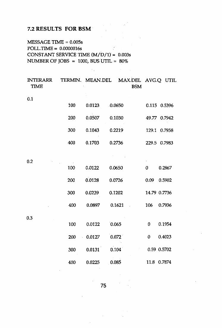
7.2 RESULTS FOR BSM

MESSAGE TIME = 0.005s POLL.TIME = 0.0000016s CONSTANT SERVICE TIME (MID/1) = 0.003s NUMBER OF JOBS = 1000, BUS 'UTTL = 80%

INTERARR TER/v[1N. MEAN.DEL MAX.DEL AVG.Q UTIL BSM TIME

0.1 100 0.0123 0.0650 0.115 0.5396

200 0.0507 0.1030 49.77 0.7942

300 0.1043 0.2219 129.1 0.7958

400 0.1703 0.2736 229.5 0.7983

0.2 100 0.0122 0.0650 0 0.2867

200 0.0128 0.0726 0.09 0.5902

300 0.0239 0.1202 14.79 0.7736

400 0.0897 0.1621 106 0.7936

0.3 100 0.0122 0.065 0 0.1954

200 0.0127 0.072 0 0.4023

300 0.0131 0.104 0.59 0.5702

400 0.0225 0.085 11.8 0.7874

75

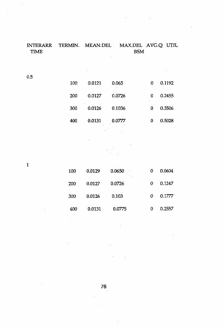
INTERARR TERMIN. MEAN.DEL MAX DEL AVG.Q UTIL TIME BSM

0.5 100 0.0121 0.065 0 0.1192

200 0.0127 0.0726 0 0.2455

300 0.0126 0.1036 0 0.3506

400 0.0131 0.0777 0 0.5028

100 0.0129 0.0650 0 0.0604

200 0.0127 0.0726 0 0.1247

300 0.0126 0.103 0 0.1777

400 0.0131 0.0775 0 0.2557

76

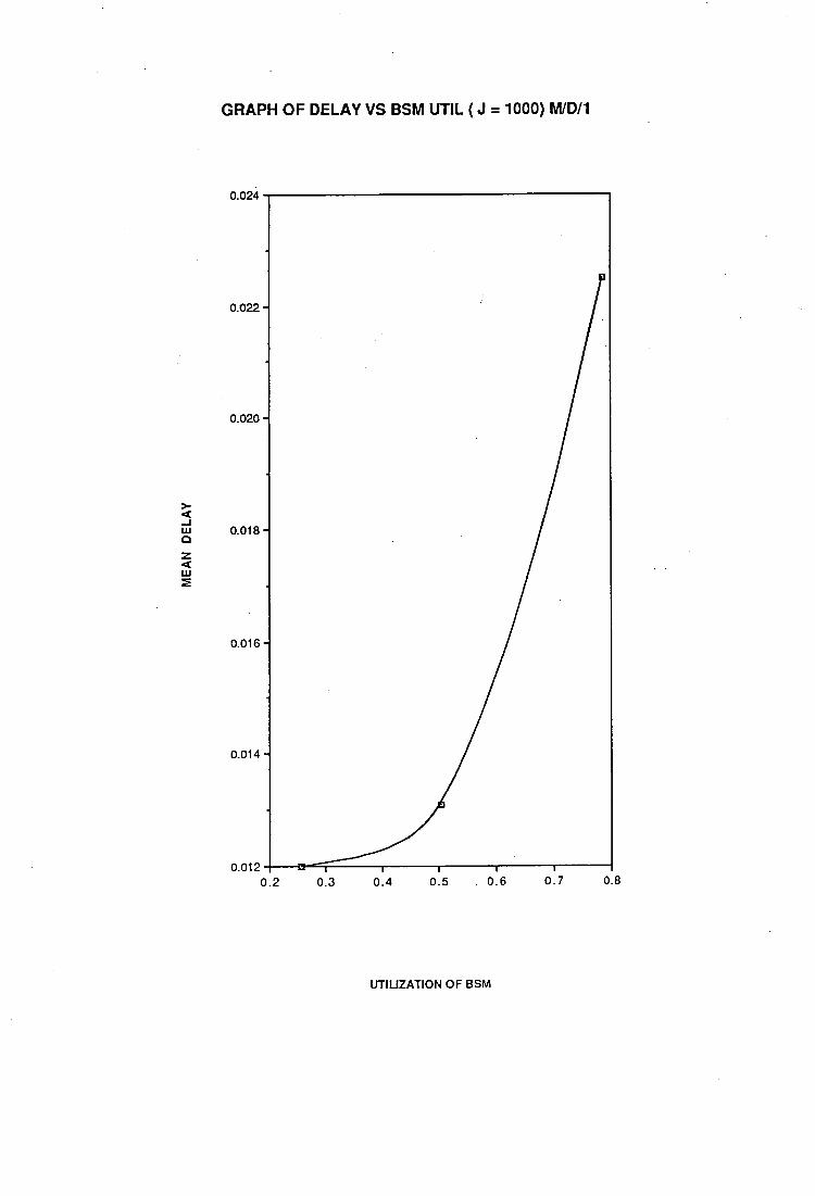
MEA

N D

ELA

Y

GRAPH OF DELAY VS BSM UTIL ( J = 1000) MID/1

0.024

02

0.3

0.4

0.5

0.6

0.7

08

UTILIZATION OF BSM

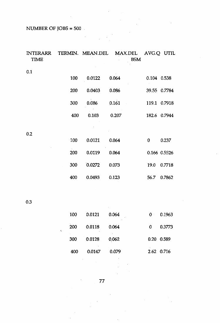
NUMBER OF JOBS = 500

INTERARR TIME

0.1

TERMIN. MEAN.DEL MAX.DEL AVG.Q U'TIL BSM

100 0.0122 0.064 0.104 0.538

200 0.0403 0.086 39.55 0.7784

300 0.086 0.161 119.1 0.7918

400 0.103 0.207 182.6 0.7944

0.2 100 0.0121 0.064 0 0.237

200 0.0119 0.064 0.166 0.5526

300 -0.0272 0.073 19.0 0.7718

400 0.0493 0.123 56.7 0.7862

0.3

100 0.0121 0.064 0 0.1963

200 0.0118 0.064 0 0.3773

300 0.0128 0.062 0.20 0.589

400 0.0147 0.079 2.62 0.716

77

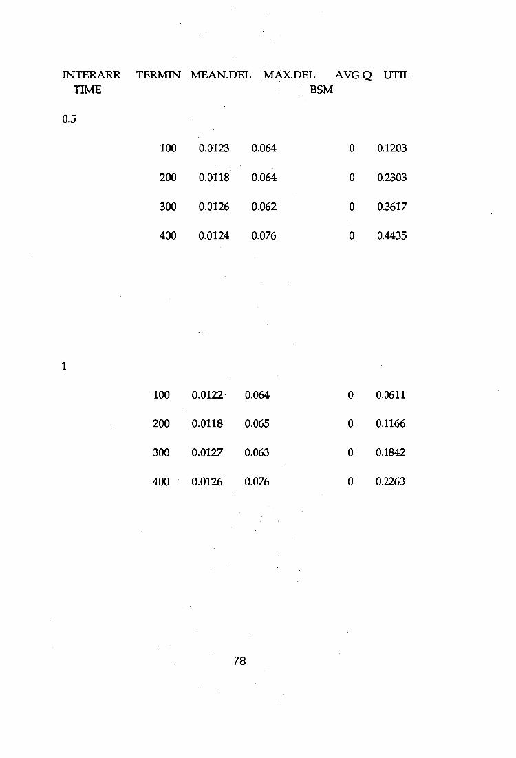
INTERARR TERMIN MEAN.DEL MAX.DEL AVG.Q UTIL TIME BSM

0.5

100 0.0123 0.064 0 0.1203

200 0.0118 0.064 0 0.2303

300 0.0126 0.062 0 0.3617

400 0.0124 0.076 0 0.4 ,435

100 0.0122 0.064 0 0.0611

200 0.0118 0.065 0 0.1166

300 0.0127 0.063 0 0.1842

400 0.0126 0.076 0 0.2263

78

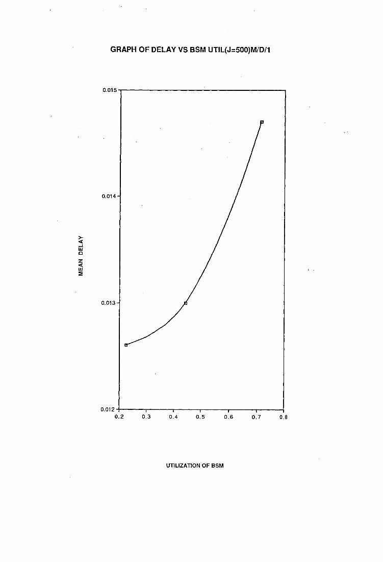
MEA

N D

ELA

Y

GRAPH OF DELAY VS BSM UTIL(J=500)M/D/1

0.015

0.014-

0.013-

0.012 0.2

0.3 0.4 0.5

0.6

0.7

08

UTILIZATION OF BSM

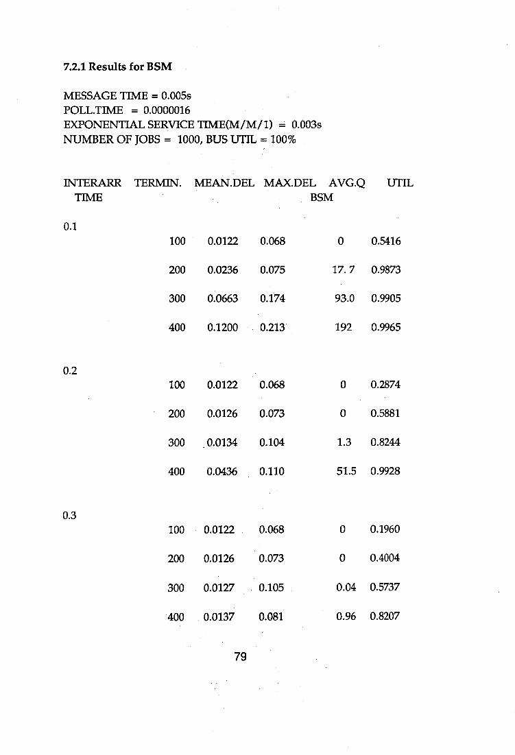
7.2.1 Results for BSM

MESSAGE TIME = 0.005s POLL.TIME = 0.0000016 EXPONENTIAL SERVICE TTME(M/M/1) = 0.003s NUMBER OF JOBS = 1000, BUS UTIL = 100%

INTERARR TIME

0.1

TERIvfIN. MEAN.DEL MAX.DEL AVG.Q BSM

UTIL

100 0.0122 0.068 0 0.5416

200 0.0236 0.075 17. 7 0.9873

300 0.0663 0.174 93.0 0.9905

400 0.1200 0.213 192 0.9965

0.2 100 0.0122 0.068 0 0.2874

200 0.0126 0.073 0 0.5881

300 0.0134 0.104 1.3 0.8244

400 0.0436 0.110 51.5 0.9928

0.3 100 0.0122 0.068 0 0.1960

200 0.0126 0.073 0 0.4004

300 0.0127 0.105 0.04 0.5737

400 0.0137 0.081 0.96 0.8207

79

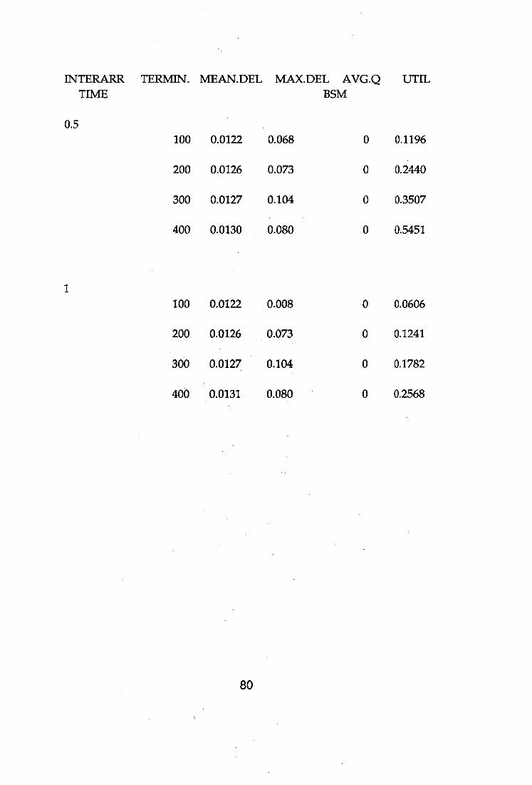
INTERARR TERMIN. MEAN.DEL MAX.DEL AVG.Q UTIL TIME BSM

0.5 100 0.0122 0.068 0 0.1196

200 0.0126 0.073 0 0.2440

300 0.0127 0.104 0 0.3507

400 0.0130 0.080 0 0.5451

100 0.0122 0.008 0 0.0606

200 0.0126 0.073 0 0.1241

300 0.0127 0.104 0 0.1782

400 0.0131 0.080 0 0.2568

80

MEA

N D

ELA

Y

GRAPH OF DELAY VS BSM UTIL(J = 1000) M/M/1

0.11

0.10 -

0.09-

0.08-

,

.,

,..

0.07 02

- 1 I • I 0.4 0.6 0.8 10

UTILIZATION OF BSM

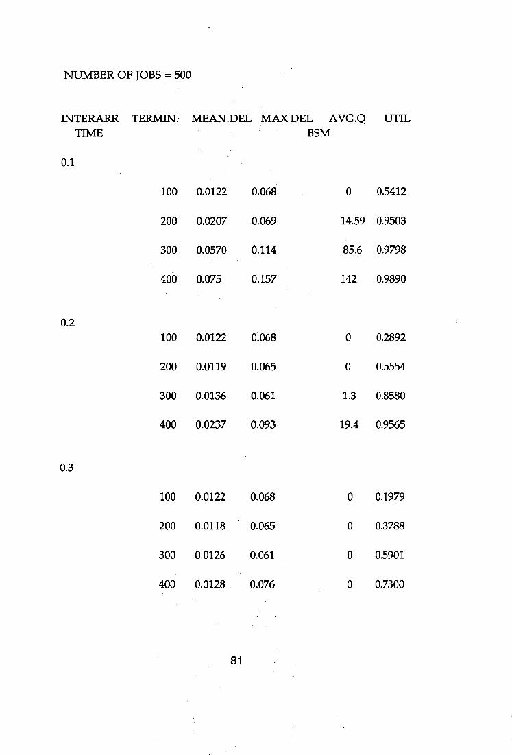
NUMBER OF JOBS = 500

INTERARR TIME

0.1

TERMIN. MEAN.DEL MAX.DEL AVG.Q BSM

UTIL

100 0.0122 0.068 0 0.5412

200 0.0207 0.069 14.59 0.9503

300 0.0570 0.114 85.6 0.9798

400 0.075 0.157 142 0.9890

0.2 100 0.0122 0.068 0 0.2892

200 0.0119 0.065 0 0.5554

300 0.0136 0.061 1.3 0.8580

400 0.0237 0.093 19.4 0.9565

0.3

100 0.0122 0.068 0 0.1979

200 0.0118 0.065 0 0.3788

300 0.0126 0.061 0 0.5901

400 0.0128 0.076 0 0.7300

81

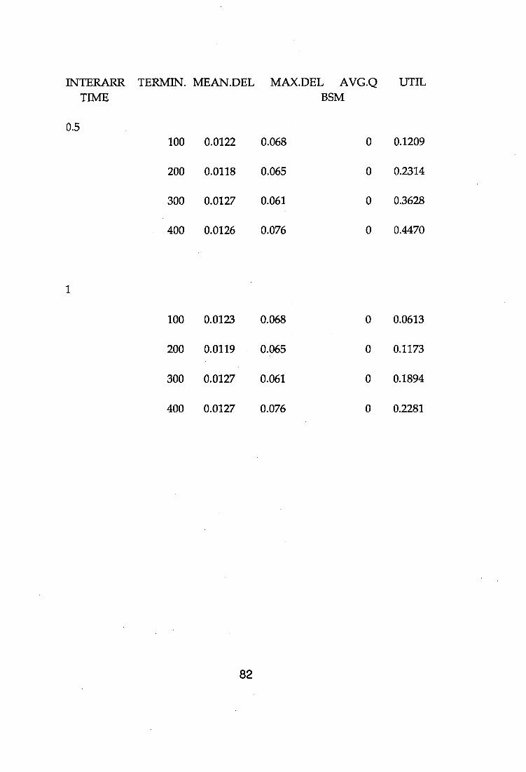
INTERARR TERMIN. MEAN.DEL MAX.DEL AVG.Q UTIL TIME BSM

0.5 100 0.0122 0.068 0 0.1209

200 0.0118 0.065 0 0.2314

300 0.0127 0.061 0 0.3628

400 0.0126 0.076 0 0.4470

100 0.0123 0.068 0 0.0613

200 0.0119 0.065 0 0.1173

300 0.0127 0.061 0 0.1894

400 0.0127 0.076 0 0.2281

82

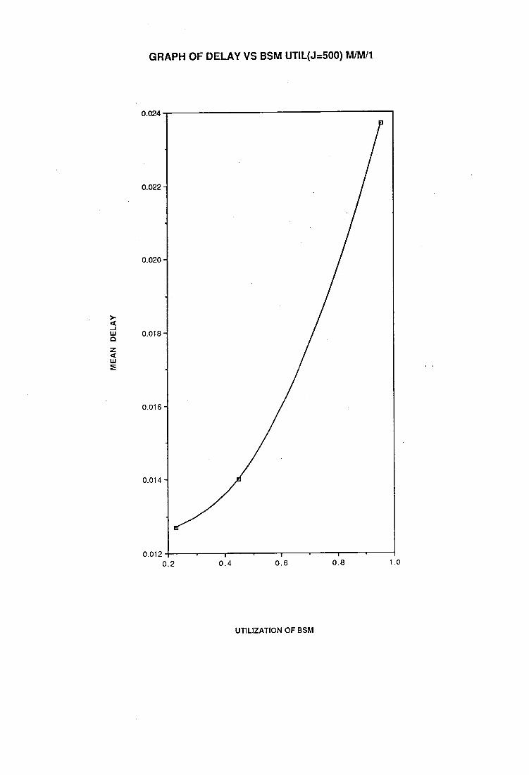
MEA

N D

ELA

Y

GRAPH OF DELAY VS BSM UTIL(J=500) M/M/1

0.024

0.022 -

0.020 -

0.018 -

0.016 -

0.014 - ..

0.012

I 0.4

1 0.8

0.2 0.6 10

UTILIZATION OF BSM

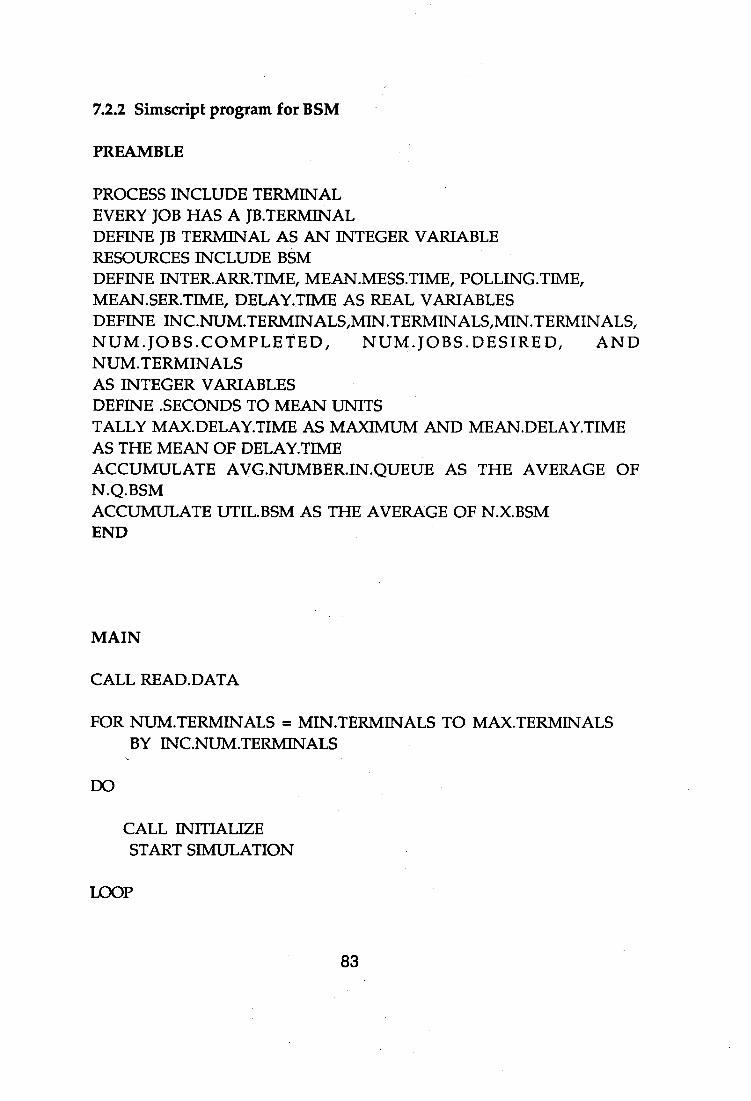
7.2.2 Simscript program for BSM

PREAMBLE

PROCESS INCLUDE TERMINAL EVERY JOB HAS A JB.TERMINAL DEFINE JB TERMINAL AS AN INTEGER VARIABLE RESOURCES INCLUDE BSM DEFINE INTER.ARR.TIME, MEAN.MESS.TIME, POLLING.TIME, MEAN.SER.TIME, DELAY.TIIVIE AS REAL VARIABLES DEFINE INC.NUM.TERMINALS,MIN.TERMINALS,MIN.TERMINALS, NUM.JOBS.COMPLETED, NUM.JOBS.DESIRED, AND NUM.TERMINALS AS INTEGER VARIABLES DEFINE .SECONDS TO MEAN UNITS TALLY MAX.DELAY.TIME AS MAXIMUM AND MEAN.DELAY.TIME AS THE MEAN OF DELAY.TIIVIE ACCUMULATE AVG.NUMBER.IN .QUEUE AS THE AVERAGE OF N.Q.BSM ACCUMULATE UTIL.BSM AS THE AVERAGE OF N.X.BSM END

MAIN

CALL READ.DATA

FOR NUM.TERMINALS = MIN.TERMINALS TO MAX.TERMINALS BY INC.NUM.TERMINALS

DO

CALL INITIALIZE START SIMULATION

LOOP

83

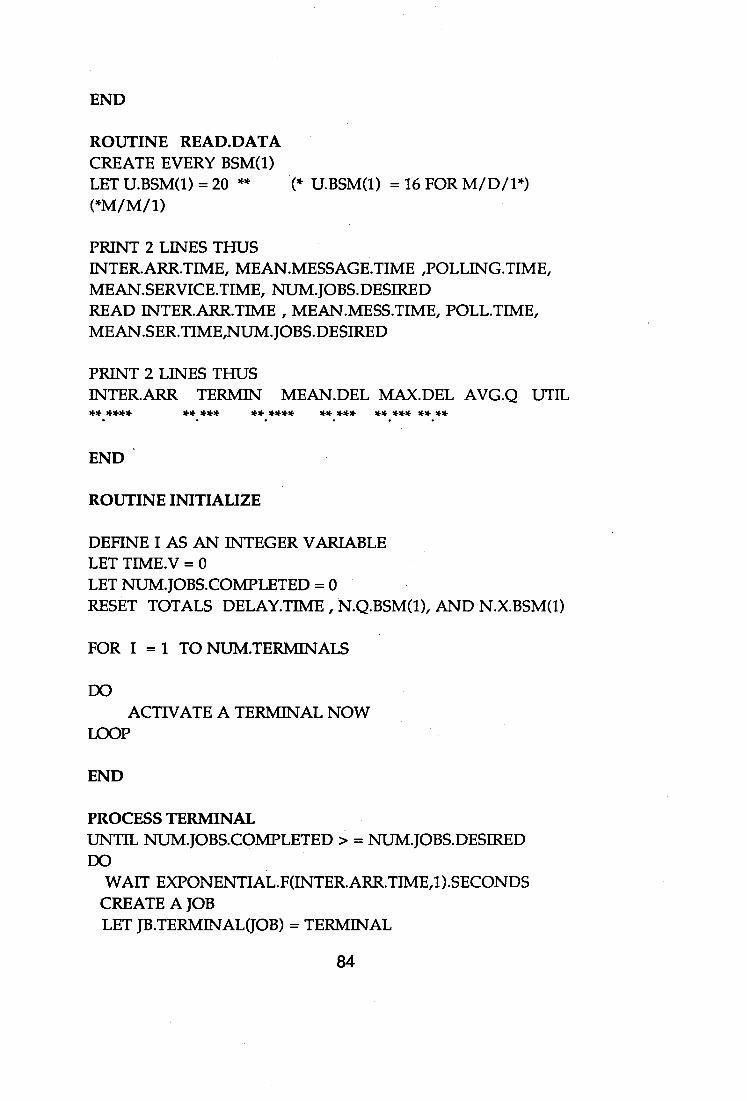
END

ROUTINE READ.DATA CREATE EVERY BSM(1) LET U.BSM(1) =20 ** (* U.BSM(1) = 16 FOR M/D/1*) (*M/M/1)

PRINT 2 LINES THUS INTER.ARR.TIME, MEAN.MESSAGE.TIME ,POLLING.TIME, MEAN.SERVICE.TIME, NUM.JOBS.DESIRED READ INTER.ARR.TIME , MEAN.MESS.TIME, POLL.TIME, MEAN.SER.TIME,NUM.JOBS.DESIRED

PRINT 2 LINES THUS INTER.ARR TERMIN MEAN.DEL MAX.DEL AVG.Q UTIL **.**** **.*** ** **** **.*** **.*** **.**

END

ROUTINE INITIALIZE

DEFINE I AS AN INTEGER VARIABLE LET TIME.V = 0 LET NUM.JOBS.COMPLETED = 0 RESET TOTALS DELAY.TIME , N.Q.BSM(1), AND N.X.BSM(1)

FOR I = 1 TO NUM.TERMNALS

DO ACTIVATE A TERMINAL NOW

LOOP

END

PROCESS TERMINAL UNTIL NUM.JOBS.COMPLETED > = NUM.JOBS.DESIRED DO

WAIT EXPONENTIAL.F(INTER.ARR.TIMEM.SECONDS CREATE A JOB LET JB.TERMINAL(JOB) = TERMINAL

84

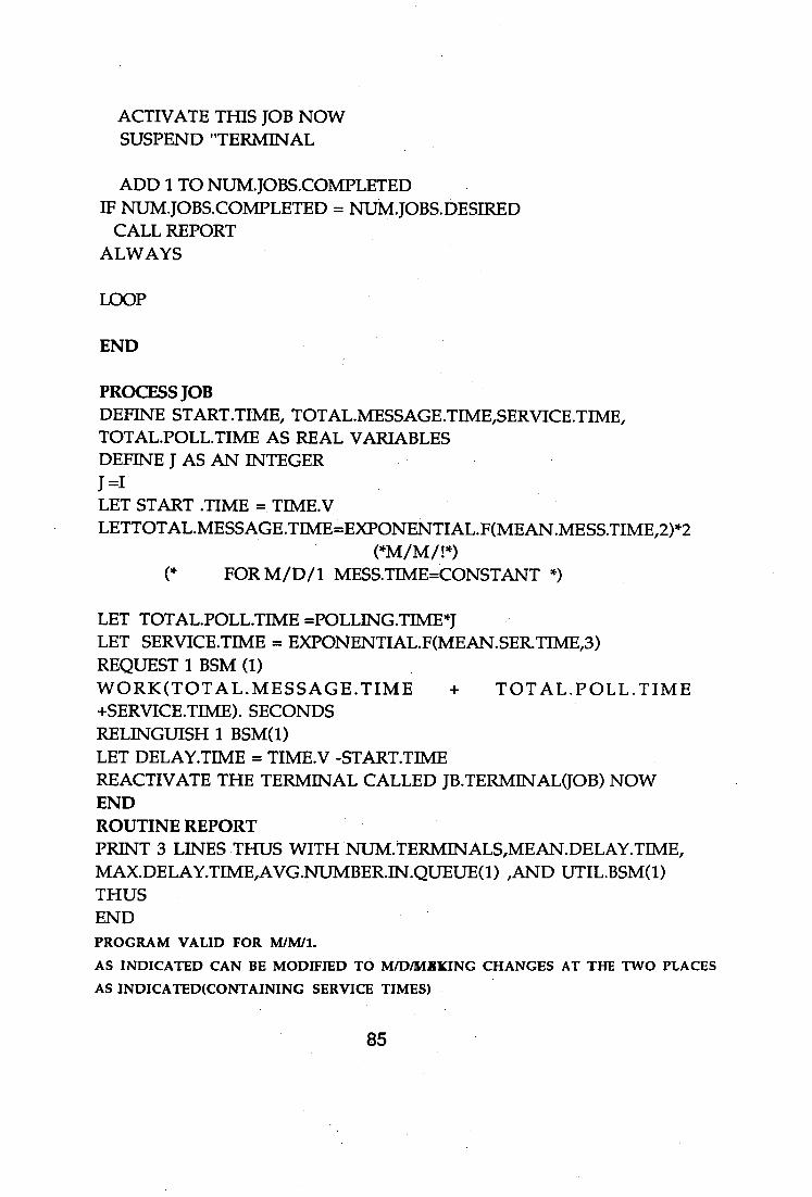
ACTIVATE THIS JOB NOW SUSPEND "TERMINAL

ADD 1 TO NUM.JOBS.COMPLETED IF NUM.JOBS.COMPLETED = NUM.JOBS.DESIRED

CALL REPORT ALWAYS

LOOP

END

PROCESS JOB DEFINE START.TIME, TOTAL.MESSAGE.TIME,SERVICE.TIME, TOTAL.POLL.TIME AS REAL VARIABLES DEFINE J AS AN INTEGER J =I LET START .TIME = TIME.V LETTOTAL.MESSAGE.TIME=EXPONENTIALF(MEAN.MESS.TIME,2)*2

(*M/M/r9 (* FOR M/D/1 MESS.TIME=CONSTANT *)

LET TOTALPOLLTIME =POLLING.TIMEI LET SERVICE.TIME = EXPONENTIAL.F(MEAN.SER.TIME,3) REQUEST 1 BSM (1) WORK(TOTAL.MESSAGE.TIME TOTAL.POLL.TIME +SERVICE.TIME). SECONDS RELINGUISH 1 BSM(1) LET DELAY.TIME = TIME.V -START.TIME REACTIVATE THE TERMINAL CALLED JB.TERMINAL(JOB) NOW END ROUTINE REPORT PRINT 3 LINES THUS WITH NUM.TERMINALS,MEAN.DELAY.TIME, MAX.DELAY.TIME,AVG.NUMBER.IN .QUEUE(1) ,AND UTIL.BSM(1) THUS END PROGRAM VALID FOR M/M/1.

AS INDICATED CAN BE MODIFIED TO M/D/MXICING CHANGES AT THE TWO PLACES AS INDICATED(CONTAINING SERVICE TIMES)

85

7.3 DESIGN FOR TSU

The performance analysis for the TSU can now be considered. A message travelling from one BSM to another has to use the facilities of the TSU. The message is sent form one BSM to the TSU via the BSM's 32Mbps packet bus. There is a switching delay within the TSU. This switching delay is assumed to be 2ms and exponentially distributed. The receiving BSM on the other side gets the message via its own 32Mpbs packet bus. There is again a waiting time in the BSM before the message is sent to the destination terminal via the 1.536Mpbs access line.

The total TSU bus capacity is defined as 8 4-32 = 256Mpbs, as a total of eight BSMs can be attached to a TSU simultaneously. However, to avoid excessive delays, the utilization of a BSM is restricted to only 80% of its full capacity. Therefore this reduces the effective switching capacity of the TSU to about 200Mpbs. The access line speed is still 1.536Mpbs. This means that the switching capacity of the TSU is about (200/1.536) = 128 times faster than that of the access line.

The various delay components can be summed up as follows as a message moves from one terminal (connected to BSM A) to another terminal (connected to BSM B). All components are exponentially distributed and the mean values are indicated for each.

Component 1. first message time (source terminal) : 8/1536 = 0.0052s 2. average half waiting time BSM (source BSM) = 0.01s 3. second message time(source BSM-TSU) = 8/3200 =0.00025s 4. waiting time in TSU = 2ms 5. second message time(TSU-BSM destin.) 8/3200 = 0.00025s 6. average half waiting time BSM(destin. BSM) = 0.01s 7. first message time (destin. terminal) = 0.0052s

86

For delay component number 2, the average half waiting time is estimated to be 0.01s. This time refers to the time taken by the message travelling only in one direction in or out of a BSM. The reasons for using 0.01s as the half waiting time will be given in the part of this report which discusses the results.

The delay component 3 refers to the time delay in the message as it is either sent to or from a TSU via the 32Mpbs packet bus. Since the message is exponentially distributed with a mean of lkbyte, the second message time is also exponentially distributed with a mean of 0.00025s.

For the performance analysis of the TSU there are interarrival times defined. They are as follows : 1. first interarrival time (mean t1, exponen. dist) for BSMs 2. second interarrival time(mean t2, exponen dist) for TSU

7.3.1 Priority for TSU traffic

There are eight BSMs connected up to the TSU. Messages will arrive at the BSMs at a certain rate. Some of these messages will be local to the BSMs. To prevent degradation of the TSU, all messages bound for the TSU, are treated with a higher priority than those local to the BSMs. This implies that to simulate this priority given to the TSU bound messages , the interarrival rate of the 8 BSMs must be equal to the interarrival rate of the TSU i.e t1 = t2.

The simulation program can then be prepared and this is given in the following pages. The program will ask for the following inputs.

1. minimum number of terminals 2. maximum number of terminals 3. increment number of terminals 4. first interarrival time t1

87

5. first message time 6. first service time (BSM) 7. number of jobs 8. second interarrival time t2 9. second message time 10.second service time(TSU)

The results obtained are examined in the discussion part of this report. The reasons why and how the interarrival times are selected are also given.

88

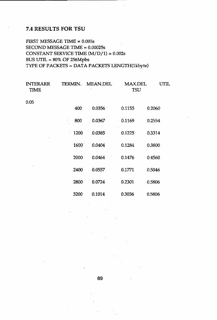
7.4 RESULTS FOR TSU

FIRST MESSAGE TIME = 0.005s SECOND MESSAGE TIME = 0.00025s CONSTANT SERVICE TIME (MID/1) = 0.002s BUS UTIL = 80% OF 256Mpbs TYPE OF PACKETS = DATA PACKETS LENGTH(1kbyte)

INTERARR TERMIN. MEAN.DEL MAX.DEL UTIL TIME TSU

0.05 400 0.0356 0.1155 0.2060

800 0.0367 0.1169 0.2554

1200 0.0385 0.1225 0.3314

1600 0.0404 0.1284 0.3800

2000 0.0464 0.1476 0.4560

2400 0.0557 0.1771 0.5046

2800 0.0724 0.2301 0.5806

3200 0.1014 0.3036 0.5806

89

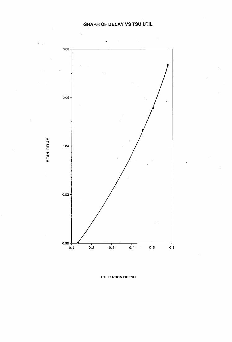
ME

AN

DE

LAY

GRAPH OF DELAY VS TSU UTIL

0.08

0.06 -

0.00 0.1 06

Pa

0.04 -

0.02 -

1 0.2 0.3 0.4 0.5

UTILIZATION OF TSU

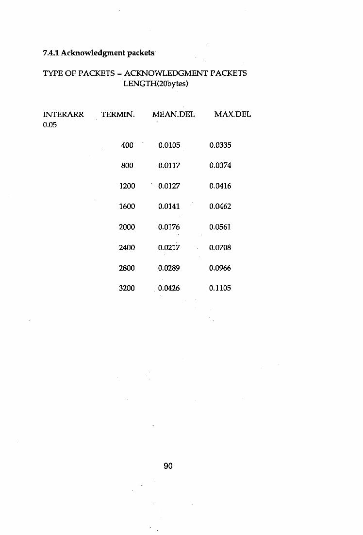
7.4.1 Acknowledgment packets

TYPE OF PACKETS = ACKNOWLEDGMENT PACKETS LENGTH(20bytes)

IN'TERARR TERMIN. MEAN.DEL MAX.DEL 0.05

400 - 0.0105 0.0335

800 0.0117 0.0374

1200 0.0127 0.0416

1600 0.0141 0.0462

2000 0.0176 0.0561

2400 0.0217 0.0708

2800 0.0289 0.0966

3200 0.0426 0.1105

90

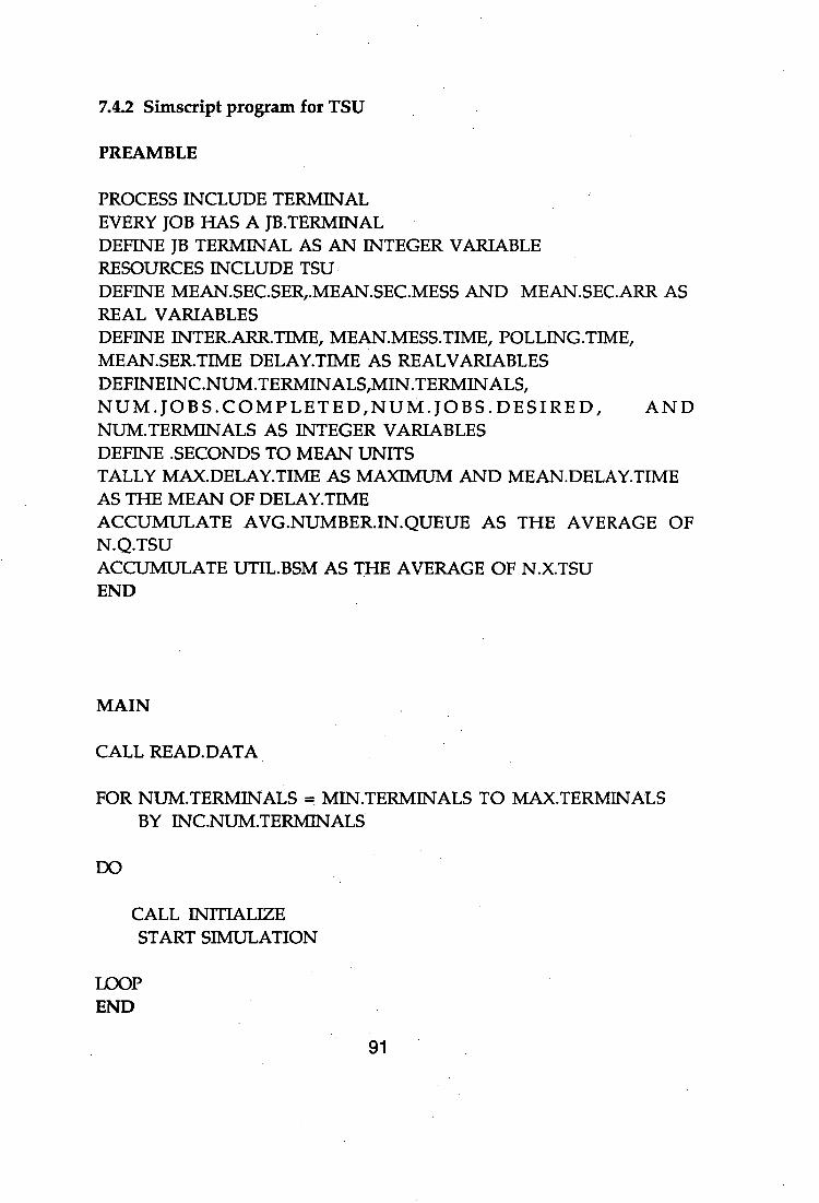
7.4.2 Simscript program for TSU

PREAMBLE

PROCESS INCLUDE TERMINAL EVERY JOB HAS A JB.TERMINAL DEFINE JB TERMINAL AS AN INTEGER VARIABLE RESOURCES INCLUDE TSU DEFINE MEAN.SEC.SER,.MEAN.SEC.MESS AND MEAN.SEC.ARR AS REAL VARIABLES DEFINE INTER.ARR.TIME, MEAN.MESS.TIME, POLLING.TIME, MEAN.SER.TIME DELAY.TIME AS REALVARLABLES DEFINEINC.NUM.TERMINALS,MIN.TERMINALS, NUM.JOBS.COMPLETED,NUM.JOBS.DESIRED, AND NUM.TERMINALS AS INTEGER VARIABLES DEFINE .SECONDS TO MEAN UNITS TALLY MAX.DELAY.TIME AS MAXIMUM AND MEAN.DELAY.TIME AS THE MEAN OF DELAY.TIME ACCUMULATE AVG.NUMBER.IN .QUEUE AS THE AVERAGE OF N.Q.TSU ACCUMULATE UTIL.BSM AS THE AVERAGE OF N.X.TSU END

MAIN

CALL READ.DATA

FOR NUM.TERMINALS = MIN.TERMINALS TO MAX.TERMINALS BY INC.NUM.TERMINALS

DO

CALL INITIALIZE START SIMULATION

LOOP END

91

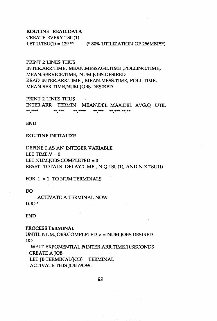
ROUTINE READ.DATA CREATE EVERY TSU(1) LET U.TSU(1) = 129 ** (* 80% UTILIZATION OF 256MBPS*)

PRINT 2 LINES THUS INTER.ARR.TIIVIE, MEAN.MESSAGE.TIME ,POLLING.TIME, MEAN.SERVICE.TIME, NUM.JOBS.DESIRED READ INTER.ARR.TIME , MEAN.MESS.TIME, POLL.TEVIE, MEAN.SER.TIME,NUM.JOBS.DESIRED

PRINT 2 LINES THUS INTER.ARR TER/VIIN MEAN.DEL M.AX.DEL AVG.Q UTIL **.**** **.*** **.**** **.*** **.*** **. **

END

ROUTINE INITIALIZE

DEFINE I AS AN INTEGER VARIABLE LET TIME.V = 0 LET NUM.JOBS.COMPLETED = 0 RESET TOTALS DELAY.TIME , N.Q.TSU(1), AND N.X.TSU(1)

FOR I = 1 TO NUM.TERMINALS

DO ACTIVATE A TERMINAL NOW

LOOP

END

PROCESS TERMINAL UNTIL NUIVIJOBS.COMPLETED > = NUIVIJOBS.DESIRED DO

WAIT EXPONENTIAL.F(INTER.ARR.TIME,1).SECONDS CREATE A JOB LET JB.TERMINAL(JOB) = TERMINAL ACTIVATE THIS JOB NOW

92

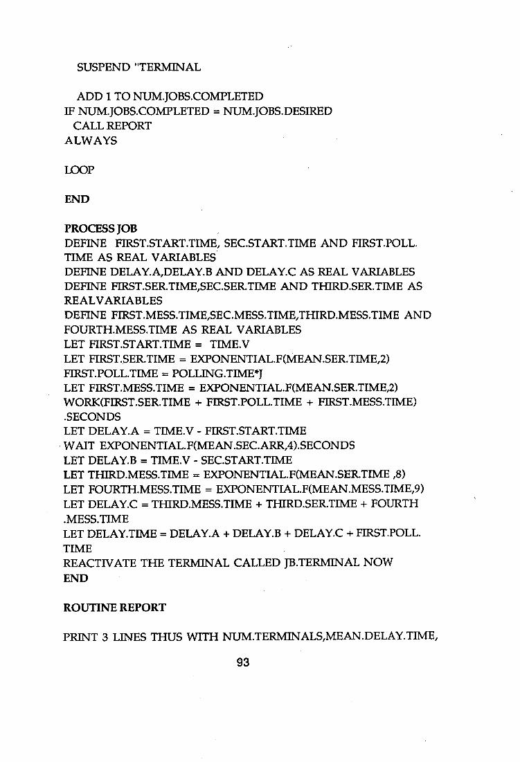
SUSPEND "TERMINAL

ADD 1 TO NUM.JOBS.COMPLETED IF NUM.JOBS.COMPLETED = NUM.JOBS.DESIRED

CALL REPORT ALWAYS

LOOP

END

PROCESS JOB DEFINE FIRST.START.TIME, SEC.START.TIME AND FIRST.POLL. TIME AS REAL VARIABLES DEFINE DELAY.A,DELAY.B AND DELAY.0 AS REAL VARIABLES DEFINE FIRST.SER.TIME,SEC.SER.TIME AND THIRD.SER.TIME AS REAL VARIABLES DEFINE FIRST.MESS.TIME,SEC.MESS.TIME,THIRD.MESS.TIME AND FOURTH.MESS.TIME AS REAL VARIABLES LET FIRST.START.TIME = TIME.V LET FIRST.SER.TIME = EXPONENTIAL.F(MEAN.SER.TIME,2) FIRST.POLL.TIME = POLLING.TIME1 LET FIRST.MESS.TIME = EXPONENTIAL.F(MEAN.SER.TIME,2) WORK(FIRST.SER.TIME + FIRST.POLL.TIME + FIRST.MESS.TIME) .SECONDS LET DELAY.A = TIME.V - FIRST.START.TIME

• WAIT EXPONENTIAL.F(MEAN.SEC.ARR,4).SECONDS LET DELAY.B = TIME.V - SEC.START.TIME LET THIRD.MESS.TIME = EXPONENTIAL.F(MEAN.SER.TIME ,8) LET FOURTH.MESS.TIME = EXPONENTIAL.F(MEAN.MESS.TIME,9) LET DELAY.0 = THIRD.MESS.TIME + THIRD.SER.TIME + FOURTH .MESS.TIME LET DELAY.TIME = DELAY.A + DELAY.B + DELAY.0 + FIRST.POLL. TIME REACTIVATE THE TERMINAL CALLED JB.TERMINAL NOW END

ROUTINE REPORT

PRINT 3 LINES THUS WITH NUM.TERMINALS,MEAN.DELAY.TIME,

93

MAX.DELAY.TIME,AVG.NUMBER.IN .QUEUE(1) ,AND UTIL.TSU(1) THUS END

94

7.5 ANALYSIS FOR QUEUING THEORY

To enhance a understanding of the simulation program used it is imperative to understand the mathematical foundation underlying the principles involved in the queuing theory[9,10,11,12].

A queue is created whenever the arrival of customers at a station is too fast as compared to the service rate offered by the server. It can be pointed out that the terminologies of 'customers' could be extended to jobs or other entities in a queue and the server could be a computer processing jobs.

7.5.1 Throughput

The efficiency of the system will depend on the output or the throughput and this is governed by the number of servers. If this number increases, the customers waiting time decreases, the queue length decreases and the system throughput increases.

To quantify the delays, queue lengths and system throughput, the following parameters can be defined :

Fy : is the interarrival time distribution ES: is the service time distribution m: the number of servers L: the number of customers Q: buffer size

The queuing discipline adopted here is based on the (FCFS) that is the 'first come first serve' principle.

95

7.5.2 Queuing parameters

The queuing parameters can be represented by an abbreviation scheme as introduced by Kendall, in the following manner:

Fy/Fs /m/q/L

where

Fy - arrival process Fs - service process m - number of servers q - buffer capacity L - customers population

The values Fy and Fs can be as follows:

M: memoryless distribution D : deterministic G : General distribution G1 : General independent distribution Er : r-stage erlang distribution Hr : r-stage hyper - exponential distribution

If the buffer capacity is assumed to be infinite, then q can be omitted and for a large infinite population , L can also be omitted. If the case of a single server is considered, then m is always 1. The representation of the queue can then be simplified and written as Fy IF /1. The simulation results

presented here are for the M/M/1 and the M/D/1 cases. The analysis will also be extended to the M/G/1 case.

96

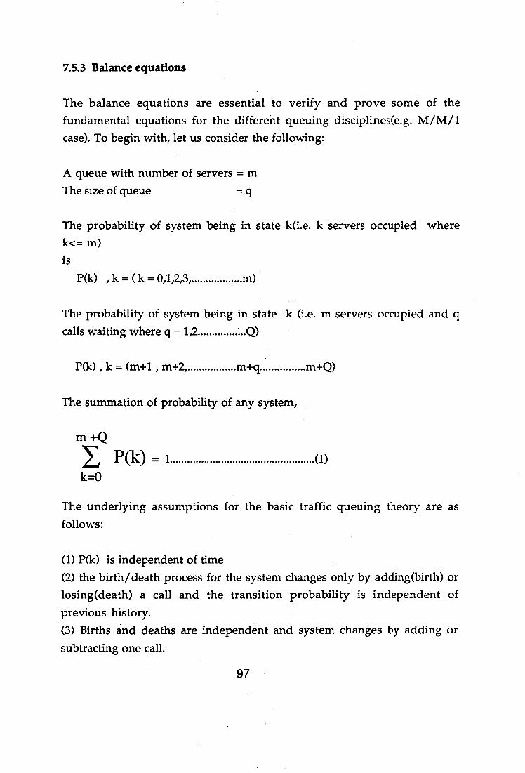
7.5.3 Balance equations

The balance equations are essential to verify and prove some of the fundamental equations for the different queuing disciplines(e.g. M/M/1 case). To begin with, let us consider the following:

A queue with number of servers = m The size of queue = q

The probability of system being in state k(i.e. k servers occupied where k<= m) is

P(k) , k = ( k = 0,1,2,3,

The probability of system being in state k (i.e. m servers occupied and q calls waiting where q = 1,2 Q)

P(k) , k = (m+1 , m+2, m+q m+Q)

The summation of probability of any system,

m +Q

P(k)=i (1) k=0

The underlying assumptions for the basic traffic queuing theory are as follows:

(1) P(k) is independent of time (2) the birth/death process for the system changes only by adding(birth) or losing(death) a call and the transition probability is independent of previous history. (3) Births and deaths are independent and system changes by adding or subtracting one call.

97

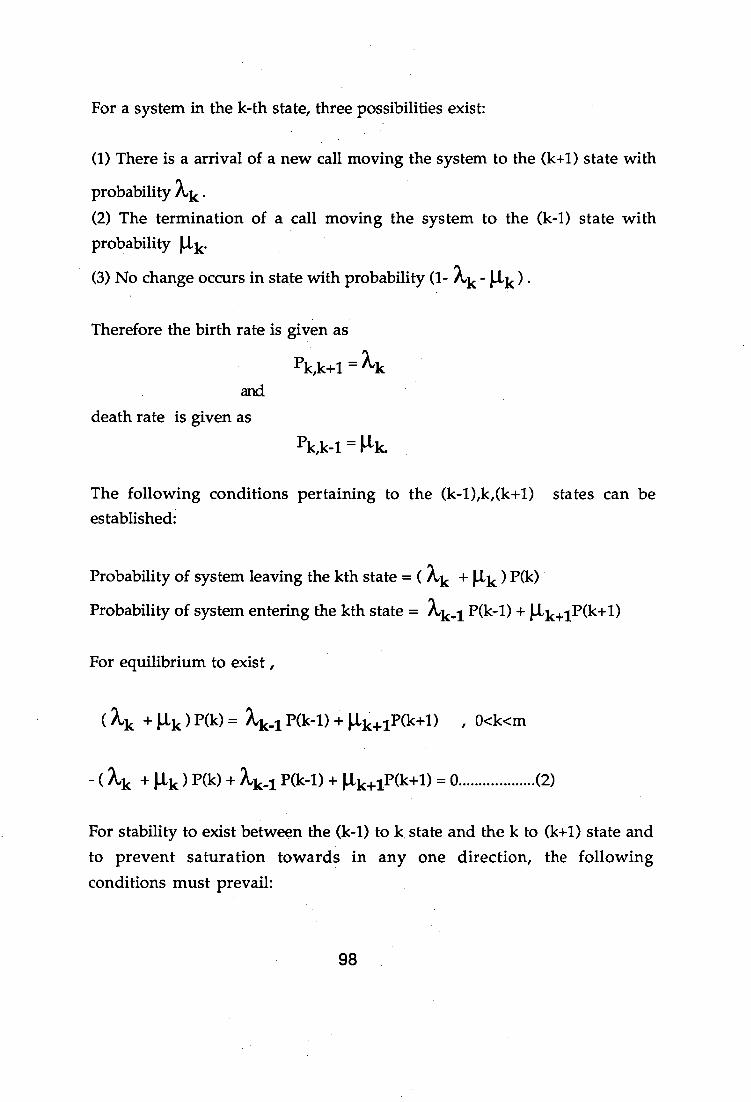
For a system in the k-th state, three possibilities exist:

(1) There is a arrival of a new call moving the system to the (k+1) state with

probability 4. (2) The termination of a call moving the system to the (k-1) state with probability

(3) No change occurs in state with probability (1- Xk - ) .

Therefore the birth rate is given as

Pk,k+1 and

death rate is given as

Pk,k-1

The following conditions pertaining to the (k-1),k,(k+1) states can be established:

Probability of system leaving the kth state = (2 k +Pk )P(k)

Probability of system entering the kth state = Xk1P(k -1) + iik+1P(k+1)

For equilibrium to exist,

(?Lk + Pk ) P(k) =Xk1 P(k-1) + p,k+ip(k+i) , 0<k<m

kk + ) P( () + 13( (-1) Ilk+1P(k+1) =0 (2)

For stability to exist between the (k-1) to k state and the k to (k+1) state and to prevent saturation towards in any one direction, the following conditions must prevail:

98

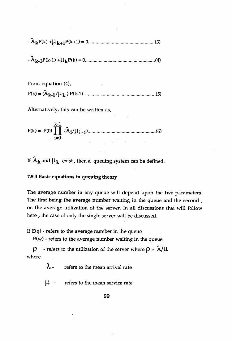
- XkP(k) +1.1,k+113(k+1) = 0 (3)

Xk-iP(k-1 ) -FilkP(k) =0 (4)

From equation (4),

P(k) = (Xk.411.1,k ) P(k-1) (5)

Alternatively, this can be written as,

k-1 P(k) = P(0) ri (xoti 1) (6)

i=0

If Xk and Pk exist, then a queuing system can be defined.

7.5.4 Basic equations in queuing theory

The average number in any queue will depend upon the two parameters. The first being the average number waiting in the queue and the second, on the average utilization of the server. In all discussions that will follow here, the case of only the single server will be discussed.

If E(q) - refers to the average number in the queue E(w) - refers to the average number waiting in the queue

p - refers to the utilization of the server where p = where

refers to the mean arrival rate

refers to the mean service rate

99

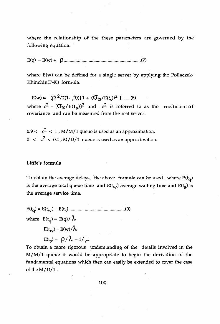
where the relationship of the these parameters are governed by the following equation.

E(q) = E(w) + p (7)

where E(w) can be defined for a single server by applying the Pollaczek-Khinchin(P-K) formula.

E(w) = (p 2/2(1- p)){ 1 + (ots/E(ts))2 1 (8)

where c2 = (6ts / E(t s ))2 and c2 is referred to as the coefficient of covariance and can be measured from the real server.

0.9 < c2 < 1 , M/M/1 queue is used as an approximation.

0 < c2 < 0.1 , M/D/1 queue is used as an approximation.

Little's formula

To obtain the average delays, the above formula can be used, where E(tq) is the average total queue time and E(t) average waiting time and E(t5 ) is the average service time.

E(t ) = E(t) + E(t5) (9)

where E(t ) = E(q)/

E(tw) = E(w)/X

E(ts) = pi X 1/ To obtain a more rigorous understanding of the details involved in the M/M/1 queue it would be appropriate to begin the derivation of the fundamental equations which then can easily be extended to cover the case of the M/D/1 .

100

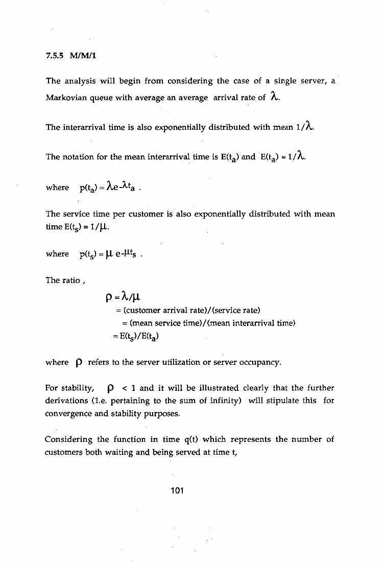
7.5.5 M/M/1

The analysis will begin from considering the case of a single server, a

Markovian queue with average an average arrival rate of X.

The interarrival time is also exponentially distributed with mean 1 /

The notation for the mean interarrival time is E(t a) and E(ta) = 1/X.

where p(ta) = .

The service time per customer is also exponentially distributed with mean time E(t) = 1/J.1.

where p(t5) = 11,

The ratio,

P =X/11 = (customer arrival rate)/(service rate)

= (mean service time)/(mean interarrival time) = E(ts)/E(ta)

where p refers to the server utilization or server occupancy.

For stability, p < 1 and it will be illustrated clearly that the further derivations (1.e. pertaining to the sum of infinity) will stipulate this for convergence and stability purposes.

Considering the function in time q(t) which represents the number of customers both waiting and being served at time t,

101

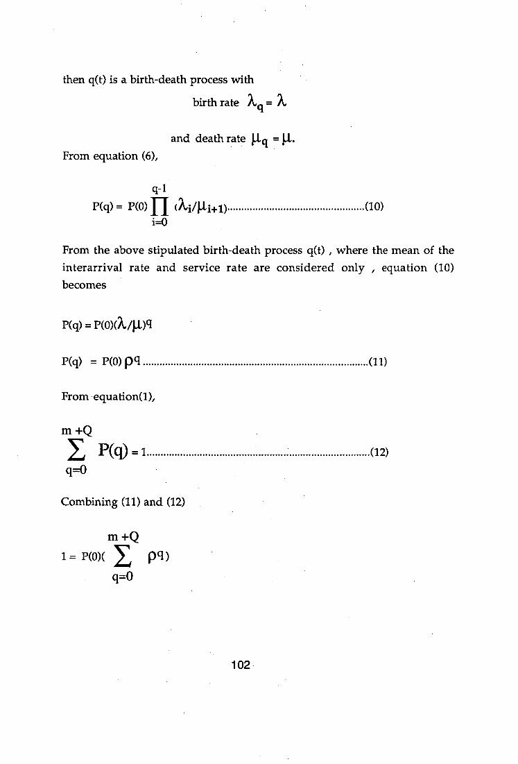
then q(t) is a birth-death process with

birth rate X, = X

and death rate I 1q = J. From equation (6),

q-1

P(q) = P(0) (10) i=0

From the above stipulated birth-death process q(t) , where the mean of the interarrival rate and service rate are considered only , equation (10) becomes

P(q) = P(0)(7/V1

P(q) = No) pq (11)

From equation(1),

m +Q

P(q) = 1 (12) q=0

Combining (11) and (12)

m +Q 1 = P(0)( pq)

q=0

102

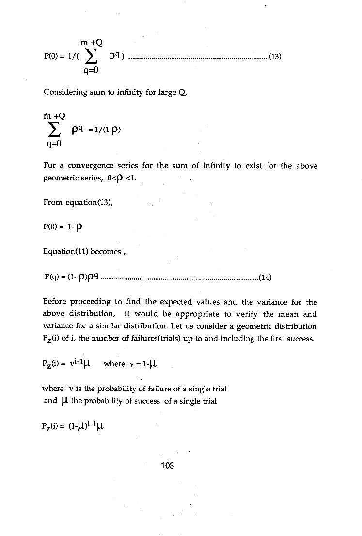
m +Q P(0)= 1/( pq ) (13)

q=0

Considering sum to infinity for large Q,

rn +Q pq .1/(1-p)

q=0

For a convergence series for the sum of infinity to exist for the above geometric series, o<p <1.

From equation(13),

P(0) = 1- p

Equation(11) becomes,

P(q) = (1- p)pq (14)

Before proceeding to find the expected values and the variance for the above distribution, it would be appropriate to verify the mean and variance for a similar distribution. Let us consider a geometric distribution P(i) of i, the number of failures(trials) up to and including the first success.

P(i) = v1411 where v = 111

where v is the probability of failure of a single trial and 11 the probability of success of a single trial

pza) = (13t)i-1 11

103

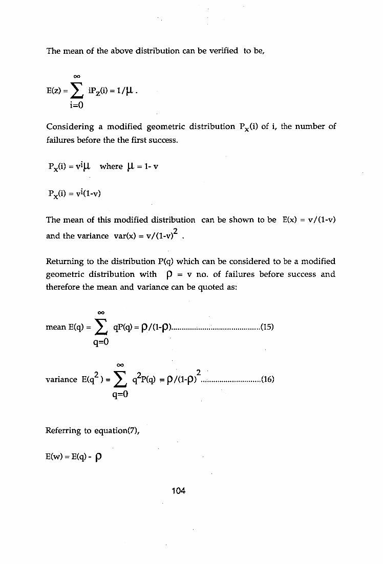
The mean of the above distribution can be verified to be,

00

E(z) = iPz(i) = 1/11

i=0

Considering a modified geometric distribution P x (i) of i, the number of

failures before the the first success.

Px(i) = v1 1 where ILL = 1 - v

P(i) = v1(1-v)

The mean of this modified distribution can be shown to be E(x) = v/(1-v)

and the variance var(x) = v/(1-v) 2 .

Returning to the distribution P(q) which can be considered to be a modified geometric distribution with p = v no. of failures before success and therefore the mean and variance can be quoted as:

00

mean E(q) = qP(q) = p/(1-p) (15) q=0

00

variance E(q2 ) = q2 P(q) 2

p/(1-p) (16)

q=0

Referring to equation(7),

E(w) = E(q) - p

104

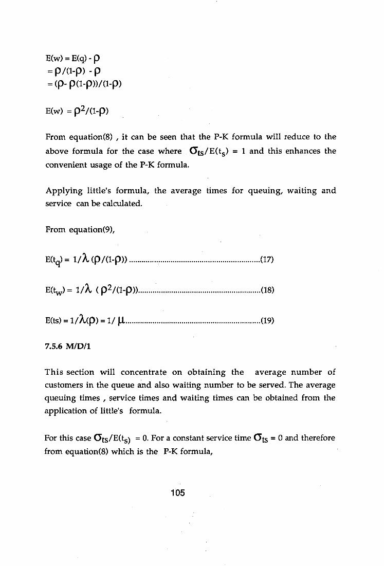
E(w) = E(q) - p = p/(1-p) - p = (p- p(1-p))/(1-p)

E(w) =

From equation(8) , it can be seen that the P-K formula will reduce to the above formula for the case where ats /E(t 5 ) = 1 and this enhances the convenient usage of the P-K formula.

Applying little's formula, the average times for queuing, waiting and service can be calculated.

From equation(9),

E(t ) = idt,(pi(1-p)) (17)

E(tw) = 1/21., ( 2/(1...)) (18)

E(ts) = 1/A(p) = 1/ 1.1 (19)

7.5.6 M/D/1

This section will concentrate on obtaining the average number of customers in the queue and also waiting number to be served. The average queuing times , service times and waiting times can be obtained from the application of little's formula.

For this case Ots E ts) = 0. For a constant service time fats = 0 and therefore from equation(8) which is the P-K formula,

105

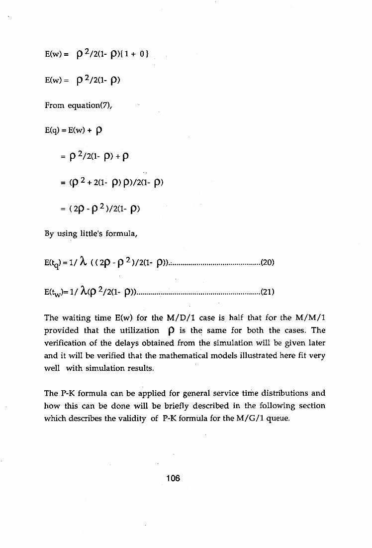
E(w) = p 2/2(1- 13)(1 o )

E(w) = p p)

From equation(7),

E(q) = E(w) + p

P 2/2(1_ p) p

(13 2 + 2(1- p) p)/2(i- p)

= ( 2p - p 2 )/2(1- p)

By using little's formula,

E(t )= 1/ ( ( 2p - p 2 )/2(1- p)) • (20)

E(t)= 1/ X(p 212(1- pp (21)

The waiting time E(w) for the MID/1 case is half that for the M/M/1 provided that the utilization p is the same for both the cases. The verification of the delays obtained from the simulation will be given later and it will be verified that the mathematical models illustrated here fit very well with simulation results.

The P-K formula can be applied for general service time distributions and how this can be done will be briefly described in the following section which describes the validity of P-K formula for the M/G/1 queue.

106

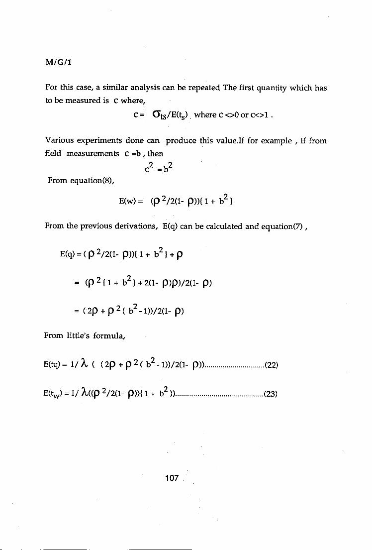
M/G/1

For this case, a similar analysis can be repeated The first quantity which has to be measured is c where,

C = /E(t ) where c <>0 or c<>1.

Various experiments done can produce this value.lf for example , if from field measurements c =b, then

c2 =b2 From equation(8),

E(w) = (p 2/2(1- p))( 1 + b2

From the previous derivations, E(q) can be calculated and equation(7) ,

E(q) = ( p 212(1-- pm 1 + b2 ) + p

cp 2 { 1 + b2 + 2(1- p)p)/2(1- p)

( 2p + p 2 ( b2 - 1))/2(1- p)

From little's formula,

E(tq) = 1/ A., ( ( 2p + p 2 ( b2 - 1))/2(1- p)) (22)

E(t) = 1/ Atop 212(1- pm I + b2 )) (23)

107

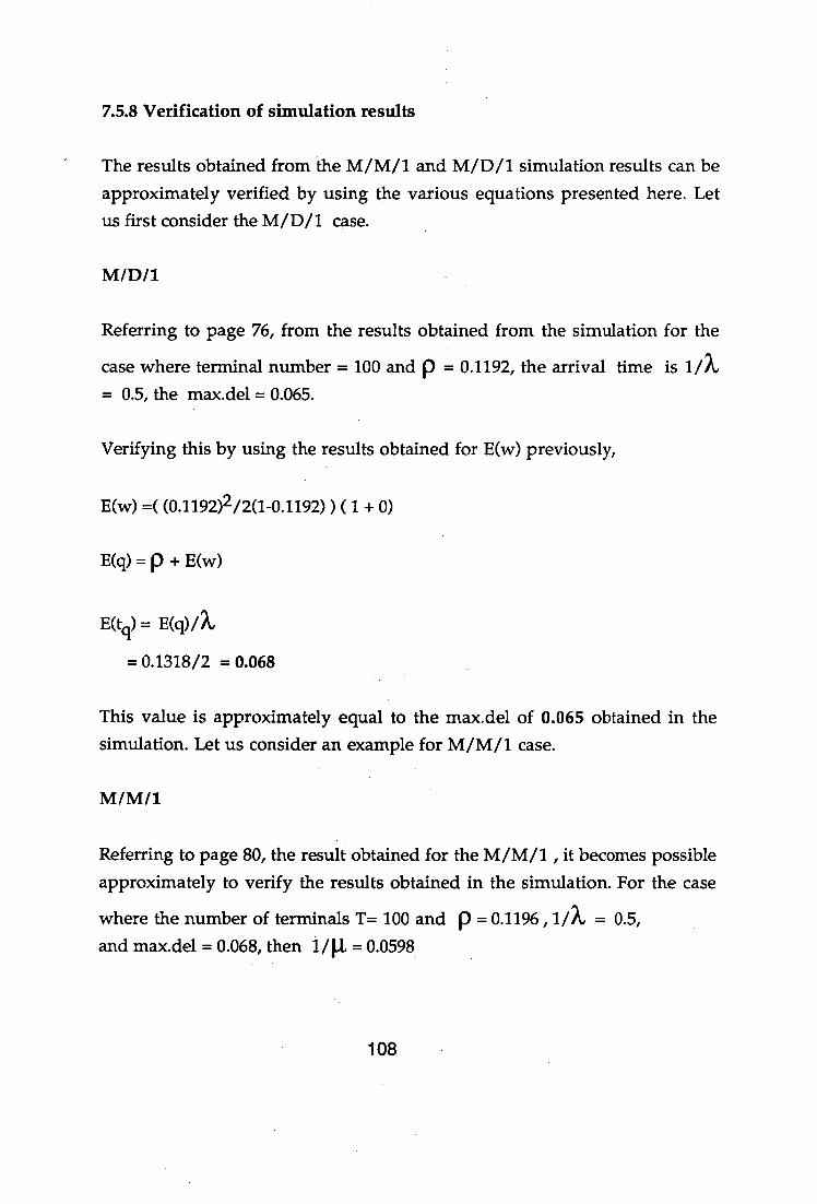
7.5.8 Verification of simulation results

The results obtained from the M/M/1 and M/D/1 simulation results can be approximately verified by using the various equations presented here. Let us first consider the MID/1 case.

M/D/1

Referring to page 76, from the results obtained from the simulation for the

case where terminal number = 100 and p = 0.1192, the arrival time is 1/k = 0.5, the max.del = 0.065.

Verifying this by using the results obtained for E(w) previously,

E(w) =( (0.1192)2/2(1-0.1192) ) ( 1 + 0)

E(q) = p + E(w)

E(t ) = E(q)/k

= 0.1318/2 = 0.068

This value is approximately equal to the max.del of 0.065 obtained in the simulation. Let us consider an example for M/M/1 case.

M/M/1

Referring to page 80, the result obtained for the M/M/1 , it becomes possible approximately to verify the results obtained in the simulation. For the case

where the number of terminals T= 100 and p = 0.1196 , 1/21., = 0.5, and max.del = 0.068, then vg = 0.0598

108

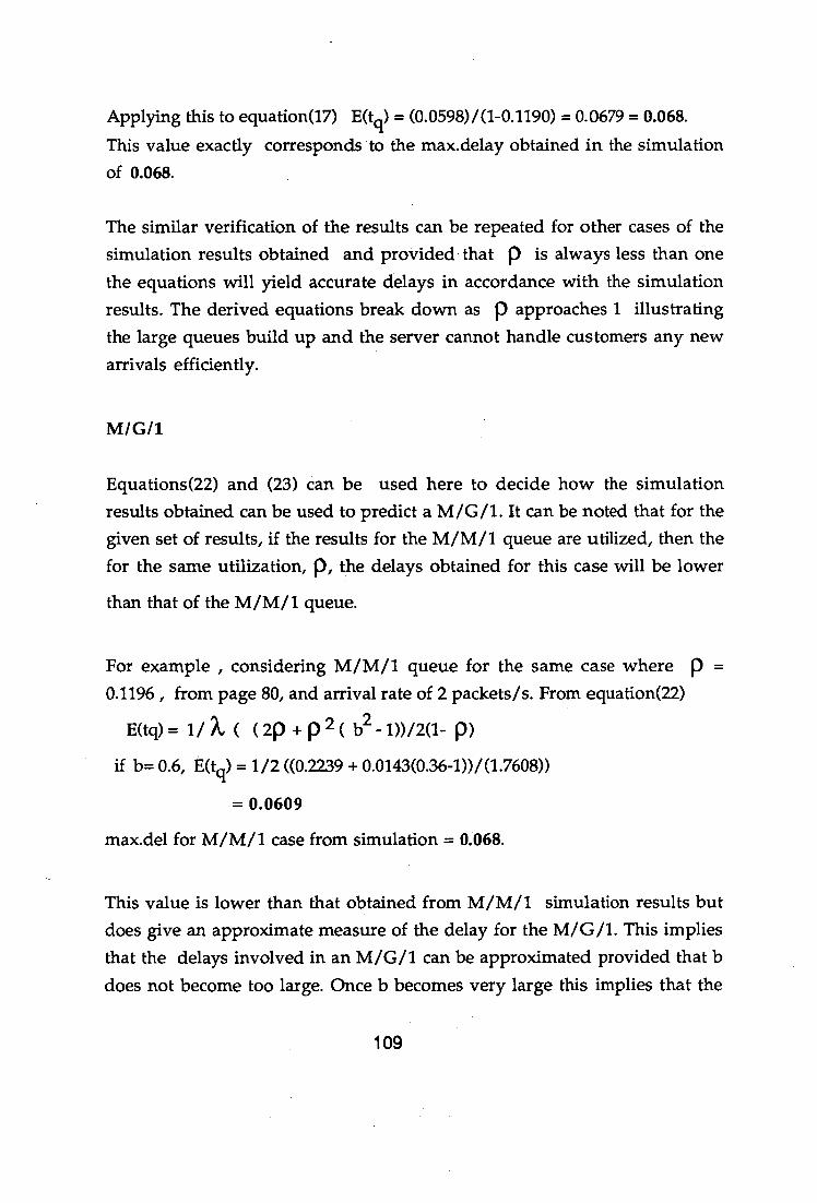
Applying this to equation(17) E(tq) = (0.0598)/(1-0.1190) = 0.0679 = 0.068.

This value exactly corresponds to the max.delay obtained in the simulation of 0.068.

The similar verification of the results can be repeated for other cases of the simulation results obtained and provided that p is always less than one the equations will yield accurate delays in accordance with the simulation results. The derived equations break down as p approaches 1 illustrating the large queues build up and the server cannot handle customers any new arrivals efficiently.

M/G/1

Equations(22) and (23) can be used here to decide how the simulation results obtained can be used to predict a M/G/1. It can be noted that for the given set of results, if the results for the M/M/1 queue are utilized, then the for the same utilization, p, the delays obtained for this case will be lower

than that of the M/M/1 queue.

For example , considering M/M/1 queue for the same case where p = 0.1196 , from page 80, and arrival rate of 2 packets/s. From equation(22)

E(tq) = 1/ X, ( 2p + p 2 ( b2 - 1))/2(1- p) if b= 0.6, E(tq) = 1/2 ((0.2239 + 0.0143(0.36-1))/(1.7608))

= 0.0609

max.del for M/M/1 case from simulation = 0.068.

This value is lower than that obtained from M/M/1 simulation results but does give an approximate measure of the delay for the M/G/1. This implies that the delays involved in an M/G/1 can be approximated provided that b does not become too large. Once b becomes very large this implies that the

109

waiting time E(w) and the delays increase drastically. Therefore, the simulation results obtained can be fitted approximately for small values of b and the simulation results tend to give a slightly higher values for the delays involved as compared to the mathematical calculations performed

as expected. The value of 'b' must be less than 0.948 so that b2 is less than 0.9(Erlang distribution). The other condition for b is that b must greater

than 0. If b is greater than 1.04 , then b2 is greater than 1.1 and this becomes a Gamma distribution having large waiting times E(tq).

Note: All calculations of time are in seconds

110

Chapter 8 : DISCUSSION

The results obtained for the BSM will be discussed first. As previously explained, the program was modified for two cases. In the first case, a exponential distribution with mean 3ms was used for the service times of the BSM, utilizing 100% of the 32Mpbs packet bus capacity. In the second case, a constant service time of 3ms was used and only 80% of the 32Mpbs packet bus was used. This was done to pin down the critical interarrival

times.

Comparing the results, the BSM utilization for the constant service was found not to exceed 80% of the bus capacity and this was expected as only 80% of the total capacity was used. As for the other case, the bus utilization was below the 100% as 100% of the bus capacity was utilized.

This implementation clearly illustrates the critical interarrival times. When the interarrival is below the 0.3s mark, the delays obtained for the constant service implementation both average and maximum are greater than that for the exponentially distributed service. The queue size are also significantly larger for the constant service implementation.. When the interarrival times are 0.5s and Is both the implementations yield similar results.This indicates that the system has stabilized if the interarrival times exceed 0.3s. The recommended interarrival time of messages from the results obtained, is 0.4s and above for each BSM.

8.1 NUMBER OF JOBS

Increasing the number of jobs also increases the utilization and delays of the system. If 500 jobs are allocated to 400 terminals, each terminal will have a average of 1.25jobs to handle. If 1000jobs are allocated to 400 terminals,each terminal has 2.5jobs to do. This affects the delays. The jobs

111

refer to the packets with a mean size of 1kbyte and exponentially distributed.

The graphs of the maximum delays versus the bus utilization (for both the constant service and exponential service) were plotted for different values of J (J = 500, J = 1000). The results indicate that the delays rise exponentially as the bus utilization increases.

The average mean delays for the BSMs interarrival times greater than 0.3s is approximately in the region of 0.013s.This delay refers to the average delay for a packet to travel from terminal A to terminal B via the BSM. It is therefore reasonable to assume that the delay experienced by the packet during half the journey is less than 0.013s.. Therefore the average half routing time of the message in the BSM in one direction, for the analysis of the TSU delays, can be said to be exponentially distributed with a mean value of 0.01s. In essence, this overestimates the delay and provides a good factor of safety margin for the delays in the BSM in one direction.

The total maximum delay experienced by the messages for the case where the interarrival time exceeds the critical interarrival time of 0.3s is about 0.1s approximately.

8.2 DESIGN OF PACKET BUFFER

The packets begin to queue up at the BSM if the messages arrive at 0.3s or less. The interarrival times are exponentially distributed. The probability

density function of the distribution, is given as P(m) = Cam where m refers to messages and a = 1/u where u represents the mean number of messages

queuing up. P(m) = Cm/u.

112

Probability density function

messages

Figure Si : PROBABILITY DENSITY FUNCTION PLOT

If the long time bit error rate is kept at 10' 7, then it becomes possible to estimate the buffer capacity of the high speed packets. Referring to Figure 8.1 , the function indicated here represents the probability density function obtained by integrating the probability p(m). Therefore, we can solve for m.

1- 0.9999999= P(m)

= 0.0000001

Taking log on both sides : -m/u = -16.1 m= 16.1u

If u = 20, then m=16.1*20 = 322 messages. This means that the packet buffer must be able to accommodate 322 messages, lkbyte long. As the mean value increases, the design becomes more expensive as more memory cells are required for the packet buffer capacity. The mean value of u = 20 is sufficient in this design operating the system at interarrival times of 0.1s, leads to packet queues at most of about 230 messages. It is advisable again to adhere to a interarrival packet times of 0.4s and above to keep the delays

P(m)

113

low.

8.3 ARRIVAL RATES FOR TSU

In the previous sections, it was explained that messages arriving at a BSM bound for a TSU are given priority over messages local to the BSM. For the performance analysis, the interarrival times t1 and t2 were set equal to each

other. The implementation can be done by having hierarchical destination addresses allocated. For example, a destination address in the frame in the frame within a token ring or ethernet set-up can have a size of six octets. One octet can be reserved for addressing the BSMs and the TSU. There are 8 BSMs which mean 3 bits within a sufficient to code all possibilities of the packet inter destination addresses. A coding scheme of 3 bits can also be allocated for the TSU. The details of this addressing scheme will be taken up shortly.

The attached results for the TSU indicate the interarrival times of 0.05s. The system was operated at lower interarrival times and the delays obtained were high. Moreover, the interarrival time of 0.05s for the TSU can be justified in the following manner. If each BSM has a interarrival time of 0.4s (above the critical value of 0.3s) , then it is reasonable to expect 8 BSMs operating together can have interarrival rates 8 times faster. A faster arrival rates indicate the the interarrival rates must be 8 times smaller 0.4/8 = 0.05s. The maximum delay obtained here is for the case of 3200 terminals where the delay is 0.3s and the bus utilization is about 58%. The plot of maximum delays versus bus utilization is given in as indicated in the design that as bus utilization increases, the delays increase exponentially.

114

8.4 FLOW CONTROL

In the X.25 LAPB layout, a flow control mechanism is defined to control congestion and throughput. The purpose of this mechanism is as follows. For example, message bound for other BSMs are sent out from terminal A to terminal B via the TSU. Terminal A can generate a large number of packets continuously, thus overcrowding the network. Moreover, if terminal B serves other ferminals at the same time, there may be a limitation imposed on the number of messages that can be sent to terminal B at one time. Without a flow control mechanism , there is no way of knowing whether the messages reached their destinations[7,8].

To solve this problem , a window mechanism is defined. Everytime a message is sent to another terminal a counter or window gets updated. After a certain threshold value a acknowledgment is sent for all the outstanding messages. For example, if the window can have 1 message outstanding, then an acknowledgment is sent for each message. If the window size is set to 7, then an acknowledgment packet is only sent after seven packets are outstanding in the window. The window mechanism then clears its window mechanism and resets the counting mechanism.

If the number of windows are small, then this restricts the throughput rate. If the window size is too large, then the network will become overcrowded and this defeats the purpose of the flow control mechanism. The window size must follow a optimum design thus maximizing the available bit rates.

In this design, the proposed acknowledgment packets have a size of 20bytes. The simulation program was used to obtain the results for the time delay of the acknowledgment packets. The packet size is very small for the acknowledgment packets and therefore the message times are reduced significantly. Moreover, the average halfway waiting time within the BSM must be lower than 0.01s , than 0.01s, the value used for high speed packet data. A value of 0.005s (BSM half waiting time) can be used and the results

115

generated for the acknowledgment packet can also be generated .

Having obtained the results for both the high speed and acknowledgment packets , it becomes possible to design a window control mechanism indicating what the window size should be.

8.5 WINDOW CONTROL DESIGN

The design (8) has stipulated a mathematical equation on the based on the average delays of both the packet and the acknowledgment packet to control the design of the flow control mechanism. The equation given is as follows:

DD + DA <= ws*PL gscp) - PL

PLAvsL - DT

Component

1. DD: Denotes average data packet delay

2. DA: Denotes average acknowledgment packet delay

3. WS : Window size 4. SL : Bit rate of access line (1.536Mbps)

5. PLD : Mean packet size (1kbyte)

6. DT : Packet processing time in upper layers(5ms)

7. p : Access line utilization

It may be argued that the maximum delays and not the average delays should be used. However, this confusion can be cleared if reference is made to the values used for "LA and PLD which are the mean values. This

suggest that for consistency purposes, the average delays are used[8].

The next question that arises is which values of DA and DD should be

considered for use in the equation. The design recommends that the values used should coincide with the following values. The BSM utilization must

be about 80% and the TSU utilization must be about 20%.

116

Referring to the section 7.4 which contains the TSU results, for the data packets, the first entry coincides with the TSU utilization of about 20%. There are 400 terminals being used here which means the bus capacity is about 32Mpbs. Moreover, only 80% of the 32Mpbs is allowed to be used. This therefore coincides with 80% utilization of a BSM.The values for DD

and DA are taken as 0.03567 and 0.0105 respectively as from the results. The

equation at the window size reduces to the following after having substituted all the values. 0.03567 + 0.0105 = WS*(0.0052)/p - 0.0057

Therefore 0.05187 = WS(0.0052)/p

The throughput is given by multiplying the utilization with the line rate. Section 8.5.1 indicates the different throughput for the different window sizes. This is followed by the graph of 'throughput vs window size' . If the line utilization is kept at about 95% , then 10 windows are required for a throughput rate of about 1.5Mpbs.

117

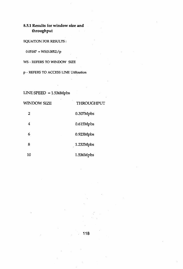
8.5.1 Results for window size and throughput

EQUATION FOR RESULTS:

0.05187 = WS(0.0052)/p

WS - REFERS TO WINDOW SIZE

p - REFERS TO ACCESS LINE Utilization

LINE SPEED = 1.536Mpbs

WINDOW SIZE THROUGHPUT

2 0.307Mpbs

4 0.615Mpbs

6 0.923Mpbs

8 1.232Mpbs

10 1.536Mpbs

118

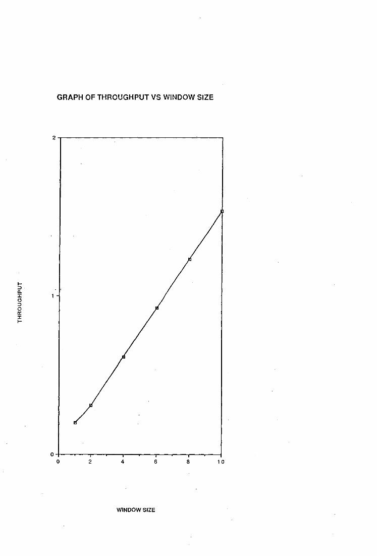
GRAPH OF THROUGHPUT VS WINDOW SIZE

2

TH

RO

UG

HP

UT

2

4

6

10

WINDOW SIZE

8.6 LINE CODES

There are essentially a few different line codes which can be adopted for the interface between the IVDT terminals and the PABX. There is a possibility of using the quaternary coding which would reduce the required bandwidth required for transmission at the SIT interface. However, to be consistent with the ISDN standards, pseudo-ternary coding must be adopted. If the primary rate standards are adopted for the S/T interface(between the IVDT terminals and the PABX), then HDB3 coding or high density bipolar can be sued. In this coding, a binary '0' is represented as a space(a no voltage condition) and a binary '1' is represented as a mark alternating according to the AMI(alternate mark inversion) principles. If the standards for the basic rate access for the SIT interface are adopted, then the'4B3T' coding can be used. In this scheme however, a binary '0' represents a mark(according to AMI) and a binary '1' represents a space(no voltage condition).

8.7 DELAYS FOR BSM AND TSU

The maximum delay experienced by a packet travelling in and out of the BSM, provided the system is operated above the critical interarrival time of 0.3s, is about 0.1s. The maximum delay experienced by a packet which travel from one BSM via a TSU to another BSM , in and out of the source and destination terminals is about 0.3s. A packet travelling in this mode has travelled across two BSMs. Since the maximum delay in the BSM is 0.1s, the delay for two BSMs is 0.1'12 = 0.2s. This delay analysis indicates that about 66% of the delay time is taken up by messages travelling in and out of BSMs. Approximately 33% of the delay is due to packets travelling in and out of the TSU (inclusive of the waiting time in the TSU).

119

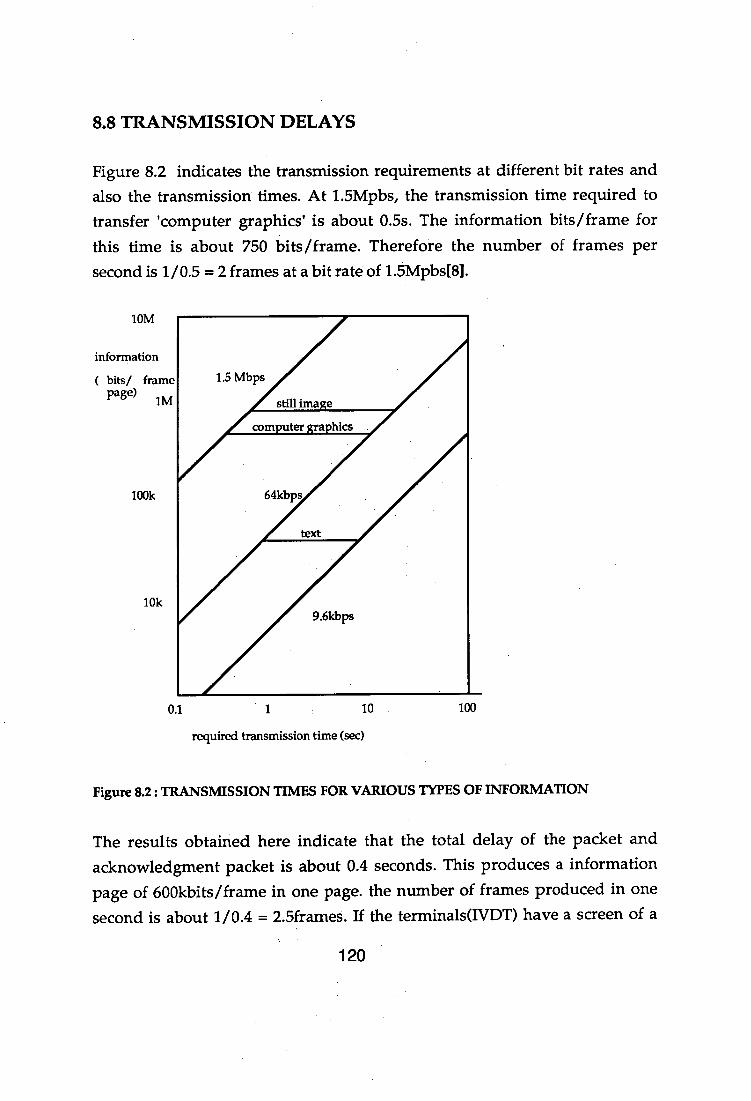
8.8 TRANSMISSION DELAYS

Figure 8.2 indicates the transmission requirements at different bit rates and also the transmission times. At 1.5Mpbs, the transmission time required to transfer 'computer graphics' is about 0.5s. The information bits/frame for this time is about 750 bits/frame. Therefore the number of frames per second is 1/0.5 = 2 frames at a bit rate of 1.5Mpbs[8].

10M

information

( bits/ frame page) lisn

100k

10k

0.1

10

100

required transmission time (sec)

Figure 8.2 : TRANSMISSION TIMES FOR VARIOUS TYPES OF INFORMATION

The results obtained here indicate that the total delay of the packet and acknowledgment packet is about 0.4 seconds. This produces a information page of 600kbits/frame in one page. the number of frames produced in one second is about 1/0.4 = 2.5frames. If the terminals(IVDT) have a screen of a

120

4:3 aspect ratio, similar horizontal and vertical resolution and 300 horizontal lines per image, then the following calculations can be done. The number of elements in each line will be (4/3)* 300 = 400 elements. the number of pixels in one frame is the 400*300 = 120000pixels. However, there are 2.5 frames per second. The total number of pixels is found to be 2.5*120000 = 300,000 pixels. The bit rate of transmission is about 1.5Mpbs and therefore the number of bits per pixel can be worked out as 1.5/0.3 = 4.5 bits/pixel. This value can be rounded of to 5bits/pixel. For a colour monitor, this value indicates that there about 30 different shades of colour codings between black and white are possible for this application.

If the transmission delay at 1.5Mpbs is 1 second instead, the number of bits per pixel is about 1.5/0.12 = 12.5 or approximately 13bits /pixel. This can yield 8000 possible colour combinations. However, here there is only one frame per second and the image produced are still images and are therefore not suitable for 'computer graphics' applications.

To improve the performance of this system, the following steps must be implemented.

1. BSM interarrival times must exceed the critical values of 0.3s.

2. The 32Mpbs packet bus utilization of the BSM must be operating at a bus utilization of less than 80% of its total capacity.

3. The packet buffer within the LIF and the TIC in the BSM must be monitored to detect any excessive build up of packet queues within the system.

4. Hierarchical addressing must be adopted within the TSU implementation to ensure that a TSU can quickly recognize the destination addresses. This will reduce the packet routing delays in the TSU.

121

8.9 PROPOSED ADDRESSING SCHEME

This point was briefly introduced in the preceding sections. If the BSMs are numbered in a order from one eight, then this will assist traffic management in the BSMs and the TSU. This type of monitoring can also enhance the operational maintenance and yield effective system management. For example, a BSM can adopt a numbering destination addresses scheme ranging from (001 to 111) reserving '000' for its own internal traffic. The TSU can adopt a destination code ranging from '000' for BSM number 1 and ending with '111' for BSM number 8. 6 bits are required, three for the BSM inter address scheme and 3 bits for the TSU addressing scheme. If BSM number 8 wants to send packets to BSM number 1 the the 6 bits will be coded as '001000'. The first three bits '001 1 (bits 1-3 of 6 bits code) indicate that message are due to BSM number 1 . A '001' code also indicates that these messages have priority over the BSM's internal traffic coded '000'. The next three bits coded '000' are the TSU's own addressing scheme independent of the BSM's addressing scheme(bits 4-6 of 6 bits code). The proposed addressing scheme is given in detail in section 8.9.1 for both the BSMs and the TSU. Terminals attached to each BSM can be automatically configured (eg. by the use of routing tables) and understand the coding scheme. In this way priority traffic for the TSU can be differentiated and routing can be efficiently done around the network. All the possible combinations of the 6 bits code are used and therefore there is no redundancy in this coding technique.

122

8.9.1 Addressing scheme adopted

ADDRESSING SCHEME FOR BSM ADDRESSES

BSM 1 2 3 4 5 6 7 8 NUM 1 000 001 010 011 100 101 110 111 2 001 000 010 011 100 101 110 111 3 001 010 000 011 100 101 110 111 4 001 010 011 000 100 101 110 111 5 001 010 011 101 000 101 110 111 6 001 010 011 100 101 000 110 111 7 001 010 011 100 101 110 000 111 8 001 010 011 100 101 110 111 000

ADDRESSING SCHEME FOR TSU

BSM NUM 1 2 3 4 5

7

TS1J ADDRESS 000 001 010 011 100 101 110 111

BIT NUMBER 1 2 3 4 5 6

6 BIT CODE * * * * *

Bits 1-3 BSM destination codes Bits 4-6 TSU destination codes for BSM

123

8.10 APPLICATION OF QUEUING THEORY

To fully appreciate the dynamics of the simulation package used here, it may be necessary to examine some of the key points involved in the queuing theory analysis.

It was previously pointed out that there are a few distributions which are commonly used to simulate the arrival rates or the service times in most simulation exercises. For this project, the arrival times are to follow the negative exponential distribution(or the poisson distribution). This distribution is quite commonly used in most queuing analysis as it does portray with a certain level of accuracy, the arrival rates for most situations. This distribution in essence,states that as the time increases, the interarrival time decreases. This implies that the arrival rate increases over a period of time. If the arrival rate at time t = 0 is 1 packet/s, as t increases this value will increase exponentially.

To suit such a distribution, a negative exponential distributed service can be defined. As the service time decreases over a period of time, the service rate increases.This distribution also seems to simulate most natural occurrences. However, the utilization is defined as p = service.time/arrival.time. There will be a point where the service time may not decrease any further while the arrival time continues to decrease. When this happens, p will increase and if p exceeds a value of

1, then the system is unstable.

_ The queuing theory analysis can be summarized in the following manner. There are three components, namely the average queue time

E(tq ) the average waiting time E(t) and the average service time E(t s ).

These values are derived from the average queue lengths by using

'Little's formula'

A further extension to the analysis can be done by using the 'Pollazeck formula' which defines the coefficient of variance C which can be

124

measured in most systems. If C = 0, then the distribution is a M/D/1 implying that the service times are constant and there is only one server while the interarrival times are exponentially distributed. When C =1, then the service times are also exponentially distributed.

For the M/D/1 distribution, the service times remain constant although the interarrival times continue to decrease.This distribution is therefore more prone to higher values of utilization and delays in comparison to a similar M/M/1. For this design,both the distributions were used to trap the critical the critical interarrival times. After repeating the simulation for both the M/D/1 and M/M/1 cases, the critical value for the interarrival times was noted to be 0.3s. It is therefore recommended that the interarrival times should be 0.4s and above. This yields a arrival rate of about 2.5 packets /s for a BSM. For the TSU , the recommended interarrival time was 0.05. This implies that the arrival rate is about 20packets/s for all the 8 BSMs. This value can be obtained by multiplying the arrival rate for one BSM by 8 i.e. 2.5*8 = 20 packets/s

Verifying these results analytically will require a considerable amount of mathematical modelling and assumptions have to be made as they are many non-constant delay components which contribute to the total delay. The simscript program used here verifies the bus utilization characteristics of both the 32Mpbs packet bus and the combined 256Mpbs bus as given in the design.

Section 7.5 summarizes the discussion involved in the mathematical principles governing the fundamental concepts involved in the queuing theory. The verification of the results obtained sgain enhance the understanding of the simulation package and the delays obtained by these two methods are highly correlated. A further extension of the simulation results to the M/G/1 case is also suggested.

125

RECOMMENDATIONS

The summary of the ISDN and LAN standards give a good understanding of some of the undelying principles involved in this thesis. The description of a modern PABX and integrated PABX further reinforces the understanding of the reference design[8].

The design illustrates only the expected simulation curves expected for the Burst Switching Unit (BSM) and the Tandem Switching Unit(TSU). Much of the intricate details involved in designing the simulation program here were based on various trial runs of simulation of which only the final suitable one is attached. The final simulation design gives a better understanding of how the system can be operated efficiently.

The following recommedations can be made from the simulation results. The critical interarrival time for the a message is found to be 0.3 per second. This implies the critical arrival rate is 3.33 packets every second. The proof of this is given by testing the simulation programs in the M/M/1 and MID/1 queues and trapping the critical interarrival time. The suggested interarrival time which would ensure the stability of the system is 0.4 seconds for each message (at each BSM) which implies that messages can arrive at a rate of 2.5 packets per second.

The above recommendation is supported by the proof given to approximately verify the results obtained from the simulation which is attached in the section 7.5 and this verifies mathematically all the simulation results obtained. A high positive correlation is said to exist between the mathematical models of the M/M/1 , M/D/1 ,the special case of the M/G/1 and the simulation results of the M/M/1 and M/D/1 queues.

126

Besides adhering to the interarrival time, it is also necessary to avoid each terminal from processing too many jobs at a time. For example, if each of the 3200 terminals were to process a average of one job initially and if this average is increased to a figure of 10, this would adversely affect the performance of the system. This is clearly illustrated in the simulation for cases of 500 and 1000 jobs where the delays increase in the later case.

Another recommendation to reduce the delays involved is to utilize hierachical addressing scheme. This can be programmed into the Tandem Switching Unit(TSU) and this information can be updated in the Burst Switching Unit(BSM). This will reduce the routing delays involved tremendously ensuring that the routing delay is insignificant as compared to the delay times obtained from the queuing theory.

127

CONCLUSION The suggested 'integrated PABX/LAN system architecture' can be easily implemented to cater for the growing demand in the office environment for different services(voice, data & computer graphics) simultaneously. The suitability of this system becomes more evident as the broadband standards for ISDN for LANs' and MANs' become more clearly defined in the near future thus paving the way for a faster and more dynamic ways to transfer information and providing the flexibility of having both audio and visual services available to the subscribers at low cost.

128

REFERENCES

[1] CCITT Recommendations V Series (1.430,1.431,) Q Series (921 , 922, 931,932)

[2]. IEEE Communications Magazine April 1990 Vol .38 No.4 pp 13-27.

[3]. IEEE Communications Magazine April 1990 Vol .26 No.6 pp 5-22.

[4]. Coporate Networks Faletti R.P,"Signalling System No.7",GLOCOM 88 PP 307-315 Vol 1.

[5]. Averill M.Law Christopher S. Larmey ,"An introduction to simulation using Simscript 11.5 ", CACI 1984.

[6]. Ericsson Sales Handbook MD110 , "MD110 Digital PABX Reference Book",Vol 1&2.

[7]. M Schwartz,"Telecommunication Networks: protocols, modeling and analysis" ,Addison Wesley 1987.

[8]. E Amada et al, "An integrated PABX/LAN System architecture", ICC' 88 pp 1533-1538.

[9]. Leonard Kleinrock, "Queueing Systems Volume I : Computer Applications", John Wiley & Sons 1976.

[10]. Leonard Kleinrock, "Queueing Systems Volume II : Computer Applications", John Wiley & Sons 1976.

[111. Kishor Shridharbhai Trivedi," Probability& Statistics With Reliability Queuing and Computer Science Applications",Prentice Hall 1982.

129

[12]. Alvin W. Drake,"Fundamentals of applied probability theory ", McGraw-Hill 1967.

[13]. Mitel Sales Handbook,"Microelectronics Handbook", Mite! 1990.

[14]. IEEE 802.2 ,"Logical Link Control", IEEE 1985.

[15]. IEEE 802.3, "CSMA/CD",IEEE 1985.

[!6]. IEEE 802.5,"Token Ring" IEEE 1985.

130