An empirical analysis of loyalty programs and private labeldemand

Jorge Florez-Acosta∗[Preliminary. Do not circulate without permission.]

February 14, 2014

Abstract

Loyalty programs (LP) are by now a predominant short-run nonprice strategy in retailing markets.Most work the same way: a member who purchases today gets a reward to be used next time shereturns to the store (or after she crosses some threshold). Previous researchers have concluded thatthe purpose of LPs as a marketing strategy is customer retention. In the grocery retailing sectorit seems to be as well the boost of private label (PL) demand. This paper empirically examinesthis conjecture. Using discrete-choice methods, I estimate brand-level demand taking into accounthousehold membership to loyalty programs. I find that although consumers give a lower value toprivate labels relative to quality equivalent national brands, loyalty programs have a positive andsignificant effect on PL choice, i.e. the marginal valuation for a PL is higher for LP members.Moreover, the more prone to subscribe to LPs a customer is, the larger her sensitivity to a priceincrease and the weaker the expected effects on PL demand.

JEL Codes: D12, L13, L22, L81.

Keywords: Grocery retailing, supermarket chains, loyalty programs, private labels,oligopolistic competition, discrete choice models, random coefficients.

∗Toulouse School of Economics, jorge.florez@tse-fr.eu. I am grateful to my supervisors Bruno Jullienand Pierre Dubois for their guidance. I also thank Fabien Bergès, Yhingua He, Laura Lasio and theparticipants of the following academic meetings: EARIE 40th Annual Conference in Evora (2013), XXVIIIJornadas de Economía Industrial 2013 in Segovia, the Seminario de Economía at Banco de la República inMedellín (Colombia) and the Applied Microeconometrics and the Econometrics Lunch Workshops at theToulouse School of Economics for helpful comments and suggestions. All errors are my own.

1

1 IntroductionRetailer own-branded products, also known as private labels (hereafter, PL),1 have becomeof big importance for the agents involved in the grocery supply chain, on the one hand,and for researchers and policy makers, on the other hand. Evidence shows that PL marketshare has been increasing steadily in the last decade and have become a good alternativefor consumers looking for better deals. For instance, in the United States PL’s marketshare attained 19.1% on sales in 2010 (Turcic et al., 2013), whereas it was even largerfor European countries such as the United Kingdom (46%), Germany (35%) and Spain(33%)(Steenkamp and Geyskens, 2013). On top of this, the European Commission reportsthat PL sales are growing around 4% per year on average (European Commission, 2011).

PL increase the rage of products available for consumers, intensifies the intra-brandcompetition and may stimulate upstream competition as well. Moreover, the fact that theyare supplied at lower prices constitute a further advantage for consumers.2 However, it haslong been recognized that PL have some negative impact as well. In particular, retailersmight be using them as a way to strengthen their position vis-à-vis manufacturers (buyerpower) and obtain better deals at the expense of suppliers’ profits.3 From this perspective,one may think that retailers strategies to boost PL demand may help increasing theirbargaining power.

One of this strategies seems to be loyalty programs (hereafter, LP), which are by now apredominant short-run practice in grocery retailing markets. The objective of this paper isto empirically examine the effects of loyalty programs on PL demand. Previous researchershave provided several explanations as to why retailers offer such costly programs. Theycan be summarized in two ways: i) consumer retention, as customers are more likely toreturn when there is a promised price reduction; and ii) the exercise market power, inparticular, the subscription requirement acts as an explicit discriminatory device. In thecase of grocery retailing, a third explanation seems to be the boost of PL demand. InFrance, for example, most supermarket chains link loyalty programs to the purchase ofprivate labels(see Table 1).4

Table 1: France: some supermarket loyalty programsRetailer Loyalty program Reward Products included

Carrefour Carte Fidelité 5% CarrefourIntermarche Avantage Carte 5%/5 PL products min. Several PLAuchan Carte Auchan 5% Auchan and NBLeclerc Carte e.Leclerc e/5 products Marque RepèreCasino Carte Casino 1 mile/3e NB and PLSource: Supermarkets web pages.

1They are retailers’ own-branded products supplied exclusively in their stores and produced by a sepa-rate manufacturer. They are produced as quality-equivalent products respective to national brands (NB),which are the regular highly advertised and generally everywhere-available products. In general, they aremore profitable for retailers than NB, even though they are of lower price.

2Evidence shows that PL are supplied at a 20% lower price on average relative to a quality-equivalentNB (Berges-Sennou, 2009).

3For further readings on this topic, see Scott-Morton and Zettelmeyer, 2004, Bergès-Sennou, 2006, andMeza and Sudhir, 2010.

4Most retailing chains give lagged rebates based on current purchases of selected PL products, condi-tional on the previous subscription to the program. Rebates are accumulated in customer’s account andafter a given time/money threshold is crossed, the acquired amount of money is given back to customersas a purchase coupons to be expended in any of the retailer’s stores. Some programs, such as that ofCasino’s, work slightly different as they give “miles” to customers according to a predetermined exchangerate, and have a catalogue where members can pick a gift according to the accumulated number of miles.

2

I estimate brand-level demand taking into account household membership to loyaltyprograms. I use a three-dimensional panel of quantities and prices for up to 13 brands ofplain yogurt, purchased from the 6 largest supermarket chains in up to 94 departmentsof France, weekly in 2006. I also observe demographic characteristics including householdmembership to supermarket LPs. In addition to the well documented challenges facedwhen estimating demand, such as the endogeneity of prices and the dimensionality prob-lems implied by the large number of brands, I also deal with the correlation between LPmembership indicator and the unobserved supermarket attributes. In a first stage of theestimation, I try some standard sets of instruments (BLP, 1995 and Nevo, 2001) to treatthe endogeneity of prices and LP membership. Yet, due to a poor performance of thosesets I overcome the endogeneity problems by computing the optimal instruments basedon Chamberlain (1987).

The dimensionality problem related to a large substitution matrix resulting from thenumerous products considered here is solved by using discrete-choice methods. In particu-lar, I estimate a random coefficients Logit model following closely the standard literature,namely, Berry (1994), Berry, Levinsohn and Pakes (1995) and Nevo(2000a, 2001).

Results confirm that private labels are, on average, less valued relative to nationalbrands. However, I find that the marginal valuation of PL products increases with sub-scription to the supermarket LP, which confirms the believe that LP serve as a way toboost store-brands demand. Moreover, when customers subscribe to several separate LPsof competing retailers, the expected effects are weaker, i.e., the marginal valuation of PLproducts decreases with the number of subscriptions and customers are more sensitive toprice changes.

I use the estimates to conduct some demand-side counterfactuals playing with thesubscription status of the customers. In a first scenario, I assume that everybody ismember of at least one loyalty program. In a second scenario, I assume the contrary:no one is member to LPs. Results support the hypothesis of this paper that LP mightbe used as a way to boost PL demand as it increases by more than 75% when former’non-loyals’5 become members (first scenario). On the other hand, in the absence of LPs(second scenario) PLs seem to be less attractive products for both former ’loyals’6 and’non-loyals’ as aggregate demand decreases by 26% in average. Welfare analysis shows thatconsumers are in general better off when they all join a LP and worse off when no oneis member to LPs, as compared with the baseline scenario. However, the second scenariohas a larger impact on consumer surplus: zero subscription to LP causes a reductionin consumer surplus that doubles the increase in consumer welfare when there is fullsubscription coverage.

There is a developed literature on topics related to either private labels, brand- andstore-loyalty or loyalty programs. However, to my knowledge this paper is the first toprovide empirical evidence on the link between supermarket loyalty programs and privatelabel demand. Table 2 summarizes the most important contributions by topic.7

This article relates in particular to Lewis (2004), who makes an evaluation of the effectsof loyalty programs based on the idea that they are addressed to “enhance [customer]retention”. Bonfrer and Chintagunta (2004) study the effects of the introduction of PL onretailers’ profits taking into account that consumers can be store- and brand-loyals. Theypropose measures for store- and brand-loyalty based on the number of trips to the same

5This is what I call those people who are not members of any LP.6Similarly, this make reference to those who are linked to supermarket LP.7For a complete survey about the theoretical and empirical literature on this theme, see Berges-Sennou

et al. (2009).

3

Table 2: Contributions to the literature on Loyalty programs and PLTopic Theory Empirics

Introduction of PL Raju et al. (1995) Bonfrer & Chintagunta (2004)Chintagunta et al. (2002)

PL demand determinants Berges et al. (2009)Competition & vertical Soberman & Parker (2006) Bonnet & Dubois (2010)relationships Bonnet & Dubois (2010)Store & brand loyalty Berges (2006)Loyalty programs Lal & Bell (2003) Bolton et al. (2000)

Lal & Bell (2003)Lewis (2004)

Lederman (2007)Coupons Caminal & Matutes (1989) Nevo & Wolfram (2002)

Cremer(1989)

store and the average “share of wallet” of a brand relative to the total expenditure onthat category of goods. They find a significant negative correlation between both typesof loyalty. Bolton, Kannan and Bramlett (2000) argue that loyalty programs membersare more likely to do repeat buying, as they weigh less than others the best outsidealternative. They conclude that LPs members are less sensitive to both quality changesand lower prices offered by competitors. Lal and Bell (2003) claim that there are tworeasons explaining the “success” of loyalty programs: (i) reduced price competition andtherefore higher profits due to switching costs, and (ii) reduced marketing expenses byfocusing attention on retaining loyal (and known) customers. This is in line with themarketing idea that promotions should be addressed to customers that are more likelyto stay. All these papers share a common basic question: What are the determinants ofcustomer retention and repeat buying? This article asks a rather different question, as theinterest is focused on the effects of loyalty programs on private label demand.

In particular, this paper closely relates to Nevo and Wolfram (2002). They provideempirical support on coupons issuing strategies by manufactures. Their objective is todescribe manufacturers’ motivations for issuing coupons. They evaluate some hypothe-ses such as price discrimination, dynamic demand effects and retailers’ pricing strategiesusing data on breakfast cereal. The key difference with my article is that I focus onretailers’ rather than manufactures’ case with the particularity that the former give cus-tomers personalized “checks” that can be expended in any set of products in stock in thesupermarket.

The remainder of this paper is structured as follows. Section 2 provides an overview ofthe theory predictions on loyalty programs. Section 3 outlines the data and a preliminaryanalysis. Section 4 sets out the empirical framework, the way I carried out the estimationprocess and presents the estimates. Section 5 displays the results of two simulated scenarioson the demand side. Finally, Section 6 concludes.

2 The theory of Loyalty ProgramsWe can summarize findings from theoretical research in two statements. First, LPs allowretailers to retain customers and induce repurchase, as long as it is a way to imposeartificial switching costs on customers and, at the same time, they are more likely to comeback when there is a promised price reduction. Second, LPs are a way to exercise marketpower, in particular, they can be used as an explicit discriminatory device as customers

4

must subscribe to the LP to be able to enjoy the benefits. In this Section, I present anoverview of the main theoretical work supporting each of those conclusions. In Section Aof the Appendix, I set out a simple two-period model which is in line with the previousliterature and that gives useful insights on the LPs effects.

Cremer (1984) addresses the question of repeat buying induced by coupons that arevalid only for next purchases of the same product, using a two-period model in whicha monopolist produces a good that consumers have not yet tasted. He finds that, asconsumers have elastic participation (they can take an outside option instead of buying thegood), the monopolist optimal strategy is to charge a lower price to repeat buyers instead ofprecommitting to a second-period price. Klemperer (1987a, 1987b) lists repeat-purchasecoupons and “frequent-flyer” programs (FPPs) as examples of artificial or contractualswitching costs that make rational customers prone to display brand loyalty as demandbecomes more inelastic and firm’s market power increases. Caminal and Matutes (1990)use a similar framework as Klemperer (1987b) but endogenize switching costs to showthat coupons valid for next period purchases perform better than price precommitmentas they allow firms to get higher overall profits and reduce the intensity of competition.

In line with these results, Chen and Pearcy (2010) develop a dynamic pricing model todetermine in which cases it is optimal to reward loyalty to retain current customers or toentice brand switching in order to attract new customers away from rival firms. They findthat for those markets in which customers do not have a strong preference for a particularbrand (because good substitutes are available or preferences are likely to change for futurechoices), firms tend to enroll them in loyalty programs to reward repeat purchases anddiscourage brand switching.

The conclusion of LPs serving as a discriminatory device follows from the expositionabove. When firms reward repeat buying, they are at the same time setting a differentiatedfuture price schedule where new customers will be charged with the full tariff whereas therepeat buyers will have a reduced one by redeeming the coupon they have got in a previousperiod.

A similar conclusion can be obtained from behavior-based price discrimination8 liter-ature (see for example Caillaud and De Nijs, 2011). Although most contributions on thistopic conclude that firms should offer lower prices to new customers, Caillaud and De Nijs(2011) get the opposite result under the assumption that some firms cannot distinguishbetween old and new customers. Hence, they reward loyalty by offering lower tariffs toprevious customers and charge full prices to the new ones.

Literature has been focused, hence, on the study of these two insights, based mainly oncoupons issuing by manufacturers and FFPs as the motivating facts. However, I claim thatother forms of rewards programs, promotions and coupons issuing made by retailers are notfully explained by the existing literature. Loyalty programs other than FFPs seem to beused for additional purposes other than customer retention or price discrimination. It is thecase of supermarket LPs in France, where rewards are linked to store-brands suggestingthat one of retailers’ main motivations to enroll customers in LPs is the boost of theirown-brands demand. An argument against this conjecture could be that when a supplierneed to boost the demand for a good, it suffices to lower its price making suboptimalthe use of indirect strategies. Yet, Caminal and Matutes (1990) provide the rationalbehind the advantages of loyalty discounts relative to price reductions. They find that aprecommitment to a second-period discount is more profitable than a precommitment toa second-period price reduction for loyal customers.9

8It consists of offering different prices to different consumers depending on their past purchases.9Another argument is given by the fact that, in a world in which store-brands are cheaper and perceived

5

3 Preliminary analysis: customer profile and the groceryretailing industry

This Section aims at giving a general view of the supermarket industry in France and thecustomer profiles, through an exploratory analysis of the data. As loyalty programs area supermarket-level rather than a product-level marketing strategy, I use data on morethan 350 different food products purchased by the households in the sample during 2006to provide some descriptive evidence on customers behavior in the presence of loyaltyprograms offered by competing supermarkets. In Section 4 I will focus on one product toassess the effects of LPs on product choice.

3.1 The data

This study uses the TNS Worldpanel data base provided by the TNS-Sofres Institute.10 Itis homescan data on grocery purchases made by a sample of 14,529 households in Franceduring 2006. These data were collected by the household members themselves with thehelp of scanning devices. As the TNS Worldpanel is a continuous panel database, theykeep most households originally sampled and renew the sample every year by changing aquarter of the households in the sample, removing those rarely reporting data or increasingthe sample size.

The data set contains information on 350 different food products from around 90retailers including hyper-, super- and mini-market stores, hard-discounters and specializedretailers. Every observation in the dataset corresponds to the purchase of a food productby a household in a given date. The entries are coded with the household identificationnumber. This is to say, if the household made purchases of a bundle of products thesame day, there will be an entry for every single product purchased with three levels ofinformation:

• Household level: size, number of children, location, income, number of cars, etc.

• Individual level: characteristics of each household member (age, height, gender,schooling, etc.).

• Product level: price, quantity, retailer info (store’s name, surface), brand, type ofproduct (PL or NB), manufacturer, etc.

Furthermore, there is information on household membership to retailers’ LPs. It is adummy variable taking on a value of one if the household is member of the retailer’s LPand zero otherwise. Unfortunately, detailed information on loyalty coupons issuing andredemption is not available.

3.2 Customer profile

Table 3 displays summary statistics on household demographics, purchases, and loyaltyinformation. The survey includes people aged between 19 and 75 years old. In average,a household consists of two to three members and has an income of around 2300 € per

as lower quality goods compared to similar national brands, additional price cuts can be interpreted as abad signal for consumers and cause the reverse effect.

10I am grateful to the Institut National de la Recherche Agronomique, INRA, for giving me access tothe data base.

6

month.11 Figure 1 displays the distribution of households across income categories. Wecan see that households are asymmetrically distributed being concentrated mainly in theupper-middle categories of income. A 75% of the households included in the dataset livein city areas of France.

A 34% of products purchased by a household are PL, which corresponds to 24.75%of its total expenditure. Moreover, the average French household members are one-stopshoppers, as they only visit one store within a week. Finally, a 85% of households aremembers to at least one supermarket loyalty program and, in average, they are subscribedto two separate programs.

Table 3: Summary statistics on household characteristics and purchasesVariable Mean Median Sd Min Max

DemographicsSize of household 2.63 2.00 1.39 1 9Live in city 0.75 1 0.43 0 1Income 2337 2100 1175 150 7000# of cars 1.47 1.00 0.82 0.00 9.00

PurchasesPrivate label purchases 0.34 0.32 0.17 0 1Total expenditure (e/day) 39.10 28.56 35.40 0.01 2,221PL share (% total exp.) 24.75 15.40 38.6 0 63.63NB share (% total exp.) 75.24 72.49 83.17 0 100

Store-related information# different stores visited the same day 1.13 1.00 0.38 1.00 7.00Duration (days) between visits 8.10 6.63 6.17 1 126LP membership 0.85 1.00 0.36 0 1# of different memberships 2.60 2 1.48 1 12

Figure 1: Households distribution per Income category, 2006

In a month households visit, in average, two different retailers and only 16.65% of thetimes they go to the store owning the LP to which the household is member. Using thisinformation along with the average duration of 1.89 months a household takes to return

11I constructed the numeric variable Income from a categorical variable that originally displays incomelevel of the household distributed in 18 income ranks. I took the average income per category and assignedthe same value to all households in the same category. See Figure 1 for further information on thedistribution of household income.

7

to the same retailer, we get seven weeks as the average duration a LP member takes to goback to its “patronized” supermarket, which is not so frequent taking into account thathousehold members go shopping at least once a week in average (see Table 4).

Table 4: Summary statistics of monthly visits to storesVariable Mean Median Sd Min Max

# different stores visited 2.27 2.08 0.98 1 9.25# visited if loyalty subscription 0.36 0 0.50 0 3Loyalty ratioa 16.83 0 25.40 0 100Duration (months) between visits 1.89 1.33 1.48 1 12aComputed as the number of visits to stores where customer is subscribed overthe total of stores visited.

“Loyal” vs. “non loyal” customers

A simple exploratory analysis of the data by subgroup of population gives no evidenceto support the hypothesis of loyalty programs as a discriminatory device. In effect, somedescriptive statistics (see Table 5) suggest no important differences between subscribersto a LP relative to non subscribers.

One can say that the fact of being a member of a LP does not say much aboutcustomer types as long as LPs are available to everybody and subscription costs might belower than benefits for most customers.12 Table 5 shows that these two groups are notonly similar in demographic characteristics, but also in consumption patterns: the portionof PL products purchased is similar in average (34%), it is so the total expenditure pertrip to the supermarket, the distribution of this expenditure between PL and NB, the factthat both are one-stop shoppers and that the average duration in days between trips to asupermarket is similar (around eight days).

Table 5: Loyals and non-loyals average characteristicsVariable LP members Non-members

% on total 85 15Size of household 2.63 2.62Income 2333 2361# of cars 1.47 1.48Private label purchases 0.34 0.35Total expenditure (e/day) 39.09 39.19PL share (% total exp.) 25.87 26.36NB share (% total exp.) 74.13 73.64# different stores visited the same day 1.12 1.12Duration (in days) between visits 8.04 8.41

To go a little further in the exploration of the data, I regressed consumer weekly expen-diture per retailer on the LP membership dummy and some demographic and supermarketcharacteristics. Table 6 displays the results. The coefficient for membership is positiveand significant telling that a customer tends to expend more in those supermarkets wherehe is subscribed to a loyalty program than in those where he is not. Another interesting

12Although it is argued that subscription to a LP is free and so it is expected from a rational consumerto always subscribe, I believe that there are several sources of costs that may not be negligible dependingon the consumer valuation of time, personal information, advertising spam, etc. It is actually an empiricalfact that not all the consumers subscribe to LPs: 15% of French households who frequent supermarketsdo not have any LP card.

8

estimates are those of number of subscriptions to different LPs and number of separateretailers visited within a week. As the descriptive statistics before suggested, people nor-mally are members of two distinct LPs in average and some of them use to be multi-stopshoppers. The estimates are both significant and negative, showing that multi subscriptionaffects negatively the expenditure in a given supermarket whereas, as expected, visitingseveral supermarkets within the same week decreases expenditure per retailer.

Table 6: Results for HH weekly expenditure per supermarketLog of total expenditure in s

Variable OLS Fixed effectsLP member 0.372 0.499

(0.003) (0.004)# of LP subscriptions -0.0477 -0.0578

(0.001) (0.001)# visits to -0.123 -0.112different retailers (0.001) (0.001)Log of Income 0.202 0.205

(0.003) (0.003)Log of age 0.109 0.104

(0.004) (0.004)HH size 0.155 0.151

(0.001) (0.001)Hypermarket 0.138

(0.003)Minimarket -0.252

(0.006)Hard-discount 0.0211

(0.004)Constant 1.099 1.151

(0.027) (0.027)adj. R2 0.145 0.179Notes: Regressions are based on 658,866 observations. The tworegressions include time dummy variables. Asymptotically robusts.e. are reported in parenthesis.

3.3 The grocery retailing industry

In France, grocery retailing is classified in three categories depending on the size of thestore: Hypermarkets, Supermarkets and Minimarkets.13 Among them, supermarkets arepreferred by most consumers: the average market share of supermarkets in terms of thetotal consumer expenditure per day is of 51.16% against 44.83% of hypermarkets and 4%of minimarkets. In terms of the daily number of visitors, supermarkets also leads theindustry: a 55.61% of the total number of customers went to supermarkets whereas a37.85% went to hypermarkets and a 6.57% to minimarkets (see Figure 2).

With respect to regular stores, Hard-discount retailers have a share of 14% on totalhousehold expenditure in groceries in a day and 16% share on total visits per day.

In terms of LP subscribers, the largest market share is 21% suggesting that the market13According to the French law, a grocery retailing store is considered a Hypermarket when, among other

characteristics, its surface is greater or equal to 2, 500m2, a Supermarket if the surface is in the interval[400, 2500) m2 and a Minimarket if the surface is in [120, 400) m2. Hard-discount stores are also includedin these three categories as they also have shops of all sizes.

9

Figure 2: Market share indicators by store size, average percentage per day, 2006

is not very concentrated.14 Still, around 75% of LP subscribers is concentrated by the fiveleading retailers (see Figure 3). Moreover, around 62% of the households have multipleLPs subscriptions (in some cases 8 in total), reason why it is necessary to look for otherindicators such as the percentage of members visiting the store in a day.

Figure 3: Percentage of subscribers to LP by retailer, 2006

In fact, the ability of retailers to attract their “loyal” customers differs from the previ-ous results. Figure 4 shows that retailer “R2” is visited by a higher percentage of its loyalcustomers than its rival “R1”, whereas the latter has a higher portion of subscribers thanthe former. Overall, the average portion of LP members visiting the retailer owning theprogram is 20.6%.15

14There are cases of retailers that have several ways/cards that serve to the same end like, for example,Carrefour that has both “Carte fidelité” and “Carte Pass”. In these cases, I aggregate up subscribers underthe same store label, e.g., Carrefour loyalty program.

15The actual names of the retailers are hidden at the request of the TNS-Sofres, the institution providingthe data.

10

Figure 4: Average percentage of loyal visitors on the total visitors per day

4 Empirical approach and resultsAs stated before, loyalty programs appear to be used by grocery retailers as a non-pricestrategy to boost private label demand. In the following I provide empirical support tothis hypothesis.

Here I follow the discrete-choice literature and estimate two models: a multinomialLogit and a random-coefficients Logit (hereafter, I will use random-coefficients Logit,mixed Logit and the full model exchangeably). The reason for conducting these twoestimations is that the Logit model is useful to take a first glance as it is easy to estimateand gives important preliminary information about the explanatory power of the variablesof interest on consumer behavior. However, as it is well known, this model has some lim-itations due to its restrictive assumptions, in particular, it gives unrealistic informationabout substitution patterns. Then, the full model although computationally challenging,is useful to make closer-to-reality inference and counterfactual analysis.

4.1 The empirical framework

Here I will basically follow the standard literature but I will introduce some new notation,given the nature of my problem. For instance, I will assume that retailers are a source ofproduct differentiation, i.e., the same brand sold by two separate retailers becomes twodifferentiated products.

Assume we observe t = 1, 2, ..., T markets and i = 1, 2, ..., It consumers per market.I define a market as a week-Department16 combination where consumer purchases areobserved. Every time a consumer goes shopping to a given supermarket s = 1, 2, ..., S,he faces a multiple-choice decision among J brands. The conditional indirect utility ofconsumer i from choosing product j at supermarket s in market t writes as

uijst = xj βi + rsλi − αipjst + ϕiMis + ηiMis × PLjs + ξj + ∆ξjt + ξs + ∆ξst + εijst (1)

where xj and rs are a K- and R-dimensional (row) vectors of observable product j and16In France, a Department (or Departement in French) makes part of the administrative division of

the national territory being the second level of the government at the local area, after the AdministrativeRegions which are groups of departments.

11

supermarket s characteristics, respectively;17 pjst is the unit price of product j in super-market s, Mis is a dummy indicating whether the individual i is a member of supermarkets loyalty program or not and PLjs is a dummy taking on 1 if j is a private label of retailers. ξj and ξs are the mean (across individuals and markets) valuations of the unobserved(by the econometrician) product and supermarket characteristics and ∆ξjt = ξjt − ξj and∆ξst = ξst−ξs are market deviations from the respective mean under the assumption thatin each market people value differently those characteristics. Finally, individual hetero-geneity enters the model through the set of individual-specific parameters (αi, βi, ϕi, ηi)and an additive separable mean-zero random shock εijst.

As Nevo (2000a, 2001), I model consumer taste parameters as a function of observedand unobserved demographics and assume that the latter are normally distributed

α

βϕη

=

αβϕη

+ ΠDi + Σvi, vi ∼ N(0, IK+3) (2)

where Di is a d × 1 vector of demographic variables, Π is a (K + 3) × d matrix ofcoefficients measuring the change in tastes with demographics, Σ is a (K+ 3)× (K+ 3) ofcoefficients and vi captures additional demographic characteristics that influence consumerchoice but are generally not included in surveys.

In addition to the characterization of the choice among J products, it is necessary tointroduce the “outside good” as consumers can decide to not purchase any of the availablebrands. Therefore, as its price is not set in response to the inside goods prices, when ageneral price increase of the J products takes place, the aggregate output may decreaseas consumers can substitute to the outside alternative (see Berry, 1994, for a detaileddiscussion ).

The indirect utility from the outside option is thus modelled in the following way

ui0t = ξ0 + π0Di + σ0vi0 + εi0t (3)

where the mean outside good characteristics ξ0, and the parameters π0 and σ0 are notidentified. The standard solution to this problem consists of normalizing them to zero.

With all these elements along with the assumption that θ = (θ1, θ2) is a vector con-taining all the parameters of the model (θ1 = (α, β, ϕ, η, λ) contains the linear parametersand θ2 = (Π,Σ) the nonlinear ones), we can rewrite the indirect utility of a consumer ifrom purchasing brand j at supermarket s in market t as the sum of two components: amean utility common to all consumers of the same type (defined here by the subscriptm = 0, 1 of “loyals” and “nonloyals”, respectively)

δmjst = xjβ + rsλ− αpjst + ϕMms + ηMms × PLjs + ξj + ξs + ∆ξjt + ∆ξst, and (4)

and a mean-zero heteroscedastic deviation, µijst + εijst with

µijst = [pjst, xj , rs,Mms,Mms × PLjs]′ ∗ (ΠDi + Σvi) , (5)

where vector of covariates is of order K × 1. This yields17Unlike product characteristics, I do not allow supermarket characteristics to interact with demographics

but introduce them as controls instead, i.e. λ is fixed rather than a random coefficient.

12

uijst = δmjst(·; θ1) + µijst(·; θ2) + εijst (6)

This general framework is best known as the random-coefficients Logit model, as thetaste parameters are allowed to vary over individuals and are determined by both observedand unobserved demographic characteristics, with some distributional assumptions on thelatter.

A key assumption of this model is that consumers choose at most one unit of the brandthat gives the highest utility. Let the following be the set of observed and unobservedvariables determining the preference for brand j at store s

Amjst(x, r, p.t, δ.t; θ2) = (Di, vi, εijst)|uijst ≥ uilkt, ∀ l = 0, 1, ..., J ; k = 0, 1, ..., S (7)

where x are the characteristics of all products, r are the characteristics of all supermarkets,and p.t and δ.t are J×S matrices of prices and mean utilities of the J products available inthe S supermarkets, respectively. Assuming ties occur with zero probability, the marketshare of the jth brand purchased from supermarket s in market t as a function of themean utility levels of all the J + 1 products, given the parameters, by group of populationm is

smjst(x, r, p.t, δ.t; θ2) =∫Amjst

dP (D, v, ε) =∫Amsjt

dP (ε)dP (v)dP (D) (8)

where P (·) denotes population distribution function. The last equality is a result of theindependence assumption of D, v and ε. The market shares in (8) can be computed bymaking assumptions on the distribution of each of the individual variables (Di, vi, εi.t).18

4.2 The yogurt data

Among all the products in the data described in Section 3, yogurt seems to be a goodcandidate to estimate the effects of LP subscription on PL demand. It matches pretty wellthe assumptions of the Logit setup in the sense that it can be considered a non-storablegood as it should be consumed soon after purchased, and consumers demand only oneunit of it at a time,19 which is also a key assumption for the empirical framework I use.

The original database of yogurt had information on purchases of 174 varieties of yogurtsold by an average of 20 separate retailers in the 94 metropolitan departments of France.In addition, different flavors are branded under the same label, which increases the di-mensionality of the space of products as long as for research purposes, such characteristicsshould be taken into account as consumer tastes might vary across flavors for the samebranded product. In the French market there are around 144 different flavors available,being 5 the average number of flavors by brand. Here we have clearly a dimensionality

18The simplest distributional assumptions on this model lead to the (aggregate) Logit model, namely,that individual heterogeneity is only accounted for by the idiosyncratic error terms, εijst, which are dis-tributed i.i.d. Type I extreme-value. In spite of its tractability and easy estimation, the Logit impliesimportant limitations as predicted substitution patterns are unrealistic. The random coefficients solvethese problems (see BLP, 1995; Nevo, 2000a; 2001).

19It is true that people do not necessarily buy only one brand of yogurt at a time, instead, they can buyseveral varieties of the same product to have different choices at home (different flavors, fruit contents,thickness, etc.). However, following Nevo (2001), I claim that an individual normally consumes one yogurt(assuming 125gr per portion) at a time, so that the choice is discrete in this sense. Of course there couldbe cases in which some people consume more than one brand of yogurt at a time. Although I believe thisis not the general case, the assumption can be seen as an approximation to the real demand problem.

13

problem coming from the large amount of yogurt brands and varieties by brand, whichwould result in a huge substitution matrix to be estimated.

To overcome this dimensionality problem, in the first place, I focused only on theplain yogurt variety and included the flavored yogurts in the outside good. Second, I keptonly the leading 6 grocery retailing chains with a loyalty program. Then, I picked the 13leading brands based on the national market shares on total sales in 2006. The aggregatemarket share of the selected brands is of 66.5%, six of them being PL, which guaranteesthe representativeness of the subsample and still keeps a reasonable variation in the data.Summary statistics on price and market shares of the selected brands are displayed inTable 7.

Table 7: Summary statistics for price and market shares of brands in sampleVariable Mean Median sd Min Max

TotalPrice (e/125gr) 0.229 0.187 0.091 0.151 0.463Market share (% on total sales) 5.113 4.092 4.386 1.816 17.960

Private labelsPrice (e/125gr) 0.174 0.170 0.019 0.151 0.203Market share (% on total sales) 3.750 4.077 1.120 2.200 4.788

National brandsPrice (e/125gr) 0.277 0.246 0.103 0.165 0.463Market share (% on total sales) 6.282 4.092 5.828 1.816 17.960

A particularity in this empirical work comes from the fact that loyalty programs areintended to be a supermarket-level program, i.e., they are a marketing strategy to makecustomers loyal to a supermarket and not necessarily to a particular brand. Therefore,the way to assess the effects of a LP on the demand for a specific product is to think of thesupermarket selling the product as a differentiation source. Put other way, each varietyshould be defined here as a supermarket-brand combination.

I generated an ID variable for identifying each brand variety as the combination of ayogurt brand and the supermarket where it was purchased from. For instance, a Danoneyogurt purchased from Casino appears in the database under the composite variety label“Danone-Casino”, whereas the same brand purchased from Carrefour is identified underthe composite variety label “Danone-Carrefour”, meaning that equally branded productsare now differentiated varieties due to the retailers. This exercise resulted in more than 120varieties, but most had a very low market share. Based on this, I kept a final subsamplewith the leading 31 varieties of brands with market shares varying between 0.9% to 5.8%and an aggregate share of 72.9%, which were purchased from the biggest 6 supermarketchains in France in 2006.20

4.3 Variables description

The data set used for the estimation of the models previously described was aggregatedto the brand level and contains information on total sales, unit price (per 125gr serv-ing), product and store characteristics and the distribution of the household demographiccharacteristics. In particular, the following variables were constructed:

20The lack of randomness of the final sample considered in this paper does not lead to inconsistentestimates of the parameter as long as I include brand-supermarket dummy variables in the estimation.See Manski and Lerman (1977) and Bierlaire, Bolduc and McFadden (2008) for a detailed discussion onconsistent estimation of choice probabilities from choice-based samples.

14

• Brand market share (Smjst): It was computed per subgroup of population of LPmembers (m = 1) and non LP members (m = 0), as the percentage of 125gr serv-ings sold in a market (in this paper a Department-week combination) on the totalpotential number of 125gr portions that could have been consumed in that market.21The serving was determined by converting volume sales originally in kg into a 125grunit which is the size best sold in France. The potential volume sales per marketwas computed by multiplying the average national plain yogurt consumption of 1.14125gr servings per person per week in 2006 obtained from the whole data of yogurtpurchases by the total population in a department.22

• Market share of the outside good (S0t): It was defined as the difference between oneand the sum of the inside products market shares.

• Price e/125gr (pjst): It was generated by dividing the total expenditure on yogurtproducts over the total servings purchased.

• LP membership × PL dummy (Mms × PLjs): It is an interaction variable betweenthe membership to LPs indicator and a dummy variable taking on the value 1 if thebrand variety is a private label and zero otherwise. It aims at capturing the marginaleffect of LP membership on private label demand.

• Other interactions of interest: the regressions include other interactions betweendemographic variables and product characteristics such as: #Subscriptions × PLdummy, which combines information on the number of separate LP cards held by ahousehold and a dummy for private label, and Price × #Subscriptions which will beuseful to see the marginal effects of a price change on loyalty programs’ members.

4.4 Estimation

The estimation of the models described in Subsection 4.1 was conducted following thestandard methods originally proposed by Berry, Levinsohn and Pakes (1995) and improvedsome years later by Nevo (2000a, 2001).

As Nevo (2000a, 2001), I control for brand and supermarket fixed-effects by includ-ing dummy variables. This implies three main differences with respect to the originalestimation algorithm by BLP: i) the dummies capture both brand and store unobservedcharacteristics, ii) brand characteristics are not anymore valid instruments, and iii) de-mand is identified without the need to characterize the supply side. I follow the standardliterature to estimate my model. Hence, in this section I will briefly describe the gener-alities of the estimation process and the main particularities of my model. For a detaileddiscussion of the estimation algorithm and the differences i) and iii) with BLP procedure,see Nevo (2000a, 2001).

21I computed the market shares by subgroup of people in order to preserve the meaning of the membershipindicator in a context of aggregate data. This also allows me to see the problem from the viewpoint ofthe treatment evaluation where the treated are those who subscribed to supermarket s LP and the nontreated are those non-member customers.

22To be sure this would be a good approximation to the population average consumption of plain yogurt,I looked for an alternative source of information: the data on average consumption on food products fromthe National Accounts by Institut National de la Statistique et des Etudes Economiques (INSEE, Comptesnacionaux, base 2000). Here the reported average quantity consumption of 125gr servings of yogurt perperson per week was 3.3217, and provided that around 34% of that number is plain yogurt, the averageconsumption of this variety per person per week is of 1.287 servings, which is similar to the one reportedby the home scan data.

15

Estimation relies on the population moment conditions given by E[h(z)′ρ(x, θo)] = 0,where z1, ..., zM are a set of instrumental variables, i.e., a set of variables which are notincluded in the main regression equation and that are correlated with some (or all) includedcovariates but not with the error term; ρ is a function of the parameters of the model andθo is the true value of the parameters.

In case we have more instruments than needed for identification (i.e. the matrix h(z)has more columns than the matrix of covariates of the model) a generalized method ofmoments estimator is obtained by solving the problem

minθρ(θ)′h(z)Λ−1h(z)′ρ(θ), (9)

where Λ is a consistent estimator of E[h(z)′ρρ′h(z)] and plays the role of the optimalweighting matrix in expression (9).

Now, according to the empirical framework explained before, once supermarket-branddummy variables are included, the error term of the model is ∆ξjt + ∆ξst which can becomputed as a function of the mean utilities δ.t, the data and the parameters. FollowingBerry (1994), this computation requires solving first for the δ.t from the system of equationsresulting from the match of observed and predicted market shares

s.t(x, r,M, p.t, δ.t; θ2) = S.t (10)

where s.t(·) is the predicted market share function defined in (8). As the system in (10)does not have a closed-form solution for the the mixed Logit case, it should be solvednumerically.

After inverting (10) in order to express δ.t as an explicit function of the observed marketshares, the error term in (9) can be defined as

ρjst = δmjst(x, r,M, p.t, S.t; θ2)− (xjβ + rsλ− αpjst + ϕMms + ηPLjs ×Mms + ξj + ξs)

The estimation of the parameters minimizing the expression in (9) is performed usinga non-linear search. Nevo (2000a) was the first to publish a MATLAB computer codewith the estimation algorithm, and nowadays several improvements have been proposedby authors who have tried to solve problems such as the accuracy of the estimates, con-vergence issuess or computational efficiency in the process. In particular, Knittel andMetaxoglou (2012) detected some problems in the optimization algorithm such as conver-gence at nonoptimal points, multiple local optima and convergence failure, which affectedthe parameter estimates with consequences for economic predictions. They propose animproved code with eleven alternative optimization routines, the possibility of runningthe nonlinear search process several times with different sets of starting values (they use50) and provide several stopping rules playing with tolerance levels. Dubé et al. (2011)offer an alternative way to estimate the model, letting aside the Nested Fixed Point (NFP)algorithm used by previous works and proposing a mathematical program with equilibriumconstraints (MPEC) which can be more accurate as it avoids some numerical computationsand performs faster compared to the NFP.

In this paper I use Knittel and Metaxoglou’s code. The algorithm works as follows:to solve for δ.t, BLP(1995) proposed a contraction mapping which uses starting values forδ and θ2 and iterates up until it stops at some value of δ determined by a stopping ruleprovided by the econometrician

δ(k+1).t = δ

(k).t + lnS.t − ln s.t(x, r,M, p.t, δ

(k).t ; θ2), (11)

16

where δ(k).t denotes the kth iterate. The starting values for θ2 can be random draws from

a particular parametric distribution, and given those values, a starting value for δ can beobtained from a Logit regression as δ(0)

.t = lnS.t − lnS0t which is obtained aftermatchingthe predicted and obserd market shares and linearizing by taking logs (see Berry, 1994).

With a value for δ and the estimates from the linear part (θ1) of the model obtainedfrom a 2SLS estimation, the error term appearing in the objective function can be com-puted and the optimization process can be performed to obtain consistent estimates ofθ2.

4.5 Optimal Instruments

As previously stated, the inclusion of brand-supermarket fixed-effects captures the unob-served brand-supermarket characteristics and then the error term of the model becomesρjst(θ) = ∆ξjt + ∆ξst, which are the group-market deviations from the mean valuationof product and supermarket unobserved characteristics, respectively. Under the assump-tion that both supply-side agents and customers observe those characteristics and, con-sequently, their decisions account for these local deviations, we have then two sources ofcorrelation with some explanatory variables.

On the one hand, we have that prices are correlated with the department deviation ofthe mean valuation of product unobserved characteristics, ∆ξjt. This problem is alwayspresent in this kind of demand estimation models, for which a set of solutions can be foundin the standard literature. According to Nevo (2000a), there are two reasons explainingthe endogeneity of prices: i) differentiated products pricing models assume that firmsknow the unobserved (by the econometrician) characteristics of the good and use them toset the prices of products, which are a function of marginal cost and a markup dependingon demographics, and ii) the specification of the model in (1) assumes that productcharacteristics are the same for all individuals, including the price, which is not consistentwith the fact that observed prices paid by consumers are different and thus, leads tomeasurement error bias. The Logit framework solves the last problem due to the meanutility structure, but the first source of correlation is still present.

On the other hand, M.s seems to be correlated with the local deviation from themean valuation of supermarket unobserved characteristics, ∆ξst. Given that this sort ofprograms are of the firm level23 and under the assumption that the choice of a LP is driven,among other things, by the supermarket choice, i.e. it depends on the consumer’s valuationof supermarket characteristics, there is some information about households subscriptiondecisions contained in the error term.

The key identifying assumption, being the population moment condition describedpreviously, requires to find some valid instruments to deal with those endogeneity prob-lems. Here, I use an approximation to the optimal instruments following BLP (1999) andReynaert and Verboven (2013).

Instrumental variables estimation for problems with conditional moment restrictionsand i.i.d observations were proposed, among others, by Kalejian (1971), Amemiya (1974,1977), and Jorgenson and Laffont (1974). Amemiya (1977) proposed the computationof the optimal instruments in a by now standard way (see equation (15) below). Thisdevelopments assumed parametric forms for the error terms. It was Chamberlain (1987)who studied the asymptotic properties of the IV estimator for nonparametric models,where all that we know is that the distribution function of the data satisfies the equality

23A customer joins the whole supermarket chain program and not only a given store or a given productcategory sell by the supermarket.

17

of the expected value of the residual to zero when multiplied by appropriate functionsof the exogenous variables, and that efficiency bounds are attained when these functionsare replaced by the optimal instruments. Finally, Newey (1990) proposed nonparamet-ric estimation methods of the optimal instruments for nonlinear simultaneous equationsmodels.

However, inefficient sets of instruments rather than optimal ones have been commonlyused by previous research in empirical IO literature to treat the endogeneity of prices.This is the case of BLP (1995), Nevo (2000a, 2001) and Dubé, Fox and Su (2012). BLP(1999) were the first to use a sort of optimal instruments computed in an approximateway, and Reynaert and Verboven (2013) propose a method to get a more accurate versionof Chamberlain’s instruments for random coefficient models.

Following Newey (1990), consider an econometric model with the following momentrestriction24

E[ρ(xi, θo)|zi] = 0 (12)

where ρ(x, θ) is a Q×1 residual vector, z are instrumental variables and θ is a p×1 vectorof parameters where θo stands for the true value of this set of parameters, and x1, ..., xn arei.i.d. observations on the data vector xi where zi makes part of its components. Assuminghomoscedasticity, the variance-covariance matrix conditional on the instrumental variablesis

E[ρ(x, θo)ρ(x, θo)′|zi] = Ω (13)

where Ω is constant. Estimation of the parameters of the model rely in principle onthe conditional moment restriction in (12). However, it implies that we have an infinitenumber of moments one of each corresponding to a given set of zi. This problem canbe solved by using functions of the data and the parameters, which reduces the set ofequations to a finite set of ordinary moment restrictions. Let h(zi) be this function, thenestimation relies now on the unconditional moment

E[h(zi)ρ(xi, θo)] = 0 (14)

The optimal instruments are a particular function h(·) that allows us to consistentlyestimate the parameters of the model and attain the efficiency bound of the asymptoticvariance-covariance matrix. This is25

h(zi) = D(z)′Ω−1 (15)

where

D(z) = E

[∂ρ.t(x, θo)

∂θ

∣∣∣∣∣zi]

(16)

According to Newey (1990), for the particular case of a single equation system wherethe residual is a scalar (as is the case of the demand model described in subsection 4.4

24For the sake of exposition in the general formulation of optimal instruments I replace panel subscriptsby a single subscript i indicating a particular observation of the data. I will go back to the usual notationwhen I derive the particular optimal IVs for the model in this paper.

25For a complete discussion about IV estimation methods of nonlinear models, optimal instruments andefficiency bounds for nonlinear models and other models of interest, see Newey (1990).

18

of this paper) the optimal instruments become h(z) = D(z)′ as in (16).26 The number ofinstruments is equal to the number of parameters to be estimated in the model θ = (θ1, θ2),where θ1 is the vector of parameters in the linear part of the model and θ2 is the vectorof nonlinear parameters, that is

E

[∂ρ.t(x, θ)∂β′

∣∣∣∣∣zt]

= E[xj |zt] = xj (17)

E

[∂ρ.t(x, θ)

∂α

∣∣∣∣∣zt]

= E[pjst|zt] = xjγ1 + rsγ2 + wjstγ3 (18)

E

[∂ρ.t(x, θ)

∂ϕ

∣∣∣∣∣zt]

= E[Mms|zt] = rsτ1 + lsτ2 (19)

E

[∂ρ.t(x, θ)

∂η

∣∣∣∣∣zt]

= E[Mms × PLjs|zt]

= E[Mms|zt]× PLjs = (rsτ1 + lsτ2)× PLjs (20)

E

[∂ρ.t(x, θ)∂θ′2

∣∣∣∣∣zt]

= E

[∂δmjst(s.t, θ2)

∂θ′2

∣∣∣∣∣zt]

(21)

The instruments resulting for the identification of β are just product observed char-acteristics which are assumed to be exogenously set by producers and supermarkets, i.e.,those attributes do not vary in response to department-specific demand shocks. As for theparameters of the endogenous variables α, ϕ and η, the instruments are the correspondingpredicted values from first-stage OLS regressions for p.t and M.s.

To compute, first, the predicted price in (18), I follow Reynaert and Verboven (2013)and assume for simplicity that marginal costs are linear and depend on product and storecharacteristics and cost shifters, w.t, and that markets are competitive so that firms setprices at marginal cost.27 However, as I do not observe any cost shifters in my homescandata set, I use average regional prices of the same product in all the 21 French admin-istrative regions (excluding the department to be instrumented from the average priceof the region it is located in) as proxies for marginal costs information. Following Nevo(2001), I claim that after controlling for brand-specific means, regional-specific valuationsare independent of product valuations of people from other regions. This implies thatin case a demand shock happens in one region, only the local price will be affected andthe others will remain equal. This guarantees the exogeneity condition of prices. Now,prices of two departments in a country are linked by common marginal costs as long asthey are produced (supplied) by the same manufacturer (retailer) or under a standardizedprocess, reason why I believe prices of the same brand in other departments contain usefulinformation on common marginal costs.28 Table B.1 in the Appendix displays first-stageresults of price regressed on average regional prices.

26The error term denoted by ρ(x, θo) corresponds to a general formulation of a model with simultaneousequations. As the model to be estimated here consists of a single equation, the ρ(·) function equals theerror term of the demand model ∆ξjt + ∆ξst. For BLP models, for instance, where demand and supplyequations are estimated simultaneously, the residual is a vector containing both the demand- and thesupply-side error terms, ρ = (ξ, ω)′.

27Reynaert and Verboven (2013) examine both perfect and imperfect competition cases and obtainsimilar results.

28Although the independence assumption seems reasonable, there may be cases were it cannot hold as,for example, a national demand shock as pointed out by Nevo (2001).

19

Second, the predicted value for the subscription decision is assumed to be a linear func-tion of supermarket characteristics and the characteristics of the loyalty program.29 Here,however, the solution cannot be as elaborated as for the problem with prices due to thelack of information, namely, I do not observe in the data set neither household consump-tion patterns before subscription nor any other additional information on the intensityof purchases motivated by loyalty rewards, the effective amount of rewards obtained byhouseholds and the rate of coupon redemption.

Given this, I collected myself some information on the characteristics of each loyaltyprogram and use them to have a very rough approximation to the predicted subscriptiondecision indicator M.s. Table B.2 in Appendix displays estimation results for the regressionof Mis as dependent variable on some covariates describing the LP characteristics set bysupermarkets, i.e. exogenous for the consumers, and controls for demographics. Althoughthe information collected is not enough to fully account for the variation in Mis, theresults are quite appealing showing that the exogenous structure of the programs havesome explanatory power. Under the argument that supermarket LPs are the same overthe whole country, most LP characteristics are not set in response to market specificdeviations of the mean valuation of the program, hence, they can be used as exogenousinstruments for a first-stage estimation of the model.

Finally, the instruments for the nonlinear parameters in (21) are more difficult tocompute as they are nonlinear functions of product characteristics and the expectation in(21) is a function of the true parameters of the demand function, namely, both linear θ1 andnonlinear θ2. This means that the instruments for the nonlinear parameters of the modelcannot be directly computed from the data and require instead a first-stage estimationof the model. Here I follow Reyneart and Verboven (2013) notation and compute the“optimal” instruments à la BLP (1999), i.e., the population moment in (21) is replaceddirectly by an approximation of the Jacobian for the delta function and not by the empiricalanalogue of the moment restriction30

1. Obtain an initial estimate for θ = (θ1, θ2). I used the sets of explanatory variablespreviously described as instruments.

2. Compute the predicted price p.t and membership indicator Mis as in equations (18)and (19) respectively.

3. Retrieve the predicted mean utility as δmjst ≡ xj β+rsλ−αpjst+ϕMms+ηPLjs×Mms

and use it to recover the predicted market shares smjst = smjst(δ.t, θ2).

4. Compute the Jacobian of the inverted market share system δmjst(s.t, θ2) as

∂δmjst(s.t, θ2)∂θ′2

∣∣∣∣∣θ2=θ2

(22)

As δ.t is an implicit function of the system of equations defined in (10), the Jacobianis computed as the product of two matrices containing the derivatives of the predicted

29Demographics are definitely key factors determining the decision to join a given LP. However, in orderto have valid instruments I exclude any variable correlated with the error term of the model.

30Reynaert and Verboven (2013) provide an algorithm to compute the optimal instruments more accu-rately by replacing the population moment by its empirical analogue and compare its performance withthose of BLP (1999) using montecarlo simulations. They conclude that the gains in efficiency are smallwhen using their proposed method whereas the computational burden increases, reason why I stick to theBLP (1999) approximate version of the optimal instruments.

20

market shares with respect to the mean valuation δ.t for each market and the derivativesof the market shares with respect to the nonlinear parameters. Nevo (2000a) provides anAppendix with all the details and a MATLAB code for the computation of the Jacobian,which is originally used in the GMM optimization process and the computation of thevariance-covariance matrix of the estimates.

4.6 Logit results

Let Smjst be the observed market share of brand j in supermarket s by subgroup ofpopulation m in market t. The market shares were computed, as indicated previously,using the potential consumption of 125gr servings of plain yogurt by the whole populationin every market t as the potential market.

Table 8 displays the results for the estimation of a Logit demand model for yogurtby regressing ln(Smjst) − ln(S0t) on the variables described in subsection 4.3 as maincovariates. Additionally, depending on the estimation method I control for product char-acteristics (columns (1) and (4)), brand fixed effects (all columns but (1) and (4)), anddemographics (columns (3), (6) and (7)). Columns (4)-(7) in Table 8 display the resultsof 2SLS regressions using instrumental variables to treat the endogeneity of prices. Asthe purpose of this subsection is purely descriptive, I deal just with the endogeneity ofprices using sets of inefficient instruments: in column (4) I use brand dummy variables,which play a similar role as BLP (1995) instruments, and in columns (5) through (7) Iuse the set of average regional prices as in Hausman (1996) and Nevo (2000a, 2001). Col-umn (4) includes brand characteristics, whereas columns (5) through (7) include brandfixed-effects, and that is why it is no longer possible to use brand dummies as instruments.Even though I do not instrument for the endogeneity of LP membership for now, I usecharacteristics of each supermarket LP as controls in all regressions.

For every IV regression I conducted a Hausman test of over identifying restrictions,which always rejects the null hypothesis of the exogeneity of instruments, even in column(7) where demographics were replaced by department dummies which are supposed tocapture local demand shocks in a better way. An explanation could be that given that thetest is distributed as a chi-square, the large number of observations will cause any modelto be rejected (Nevo, 2001). However, the IVs are individually and jointly significant at1% level and the high first-stage R-squareds and F -statistics suggest that they have somepower (Nevo, 2001).

A result of special interest is the estimate for the interaction LPmember×PLdummy.In all regressions, the coefficient is positive and significant, and the estimate does not varyimportantly when adding demographic controls, further interaction variables or when theprices are instrumented. The coefficient means that the marginal valuation of PL productsincreases with the subscription to the supermarket owning the brand. In other words, LPsubscription has a positive impact on the demand for PLs, supporting the hypothesis ofsupermarket chains benefiting from this kind of programs as a way to boost PL demand.

Additionally, regressions (3) and (6) include the interactions Price×#Subscriptionsand #Subscriptions × PLdummy. On the one hand, the former has a negative andsignificant coefficient but it will be positive in the full model with optimal instruments,which suggests that there is a downward bias in the estimate maybe coming from theuse of inefficient instruments for price. On the other hand, the latter interaction has anegative coefficient indicating that the marginal valuation of PL products decreases withthe number of LP subscriptions. This means that multi subscription weakens the effectsof LPs on private label demand.

21

Table 8: Results from Logit for PL demandaOLS IV

Variable (1) (2) (3) (4) (5) (6) (7)Price(e/125gr) -4.345 -6.216 -4.502 -11.18 -7.335 -5.965 -6.386

(0.094) (0.114) (0.159) (1.181) (0.280) (0.463) (0.196)LP membership -0.298 -0.282 -0.252 -0.438 -0.300 -0.281 -0.268

(0.018) (0.016) (0.015) (0.032) (0.017) (0.018) (0.011)PL dummy -0.405 -0.140 -0.504 -1.149 -0.460 -0.637 -2.049

(0.025) (0.052) (0.062) (0.131) (0.088) (0.074) (0.066)LP membership×PL dummy 0.255 0.236 0.210 0.366 0.249 0.235 0.151

(0.025) (0.023) (0.022) (0.034) (0.023) (0.023) (0.015)Plastic -0.451 -2.024

(0.034) (0.273)Sugar -0.125 -0.402

(0.020) (0.051)Wholemilk 0.133 0.155

(0.011) (0.012)#Subscriptions×PL dummy -0.0561 -0.0974

(0.015) (0.019)Price×#Subscriptions -0.696 -0.396

(0.056) (0.102)Average HH size 0.181 0.167

(0.009) (0.010)Log income -1.055 -1.050

(0.023) (0.023)Car 1.306 1.287

(0.064) (0.064)# stores visited the 0.110 0.105same week (0.038) (0.038)# of trips to the same 0.0357 0.0412store within a month (0.010) (0.010)Constant -12.28 -35.37 -17.45 -5.888 -34.78 -16.91 10.54

(0.284) (0.560) (0.680) (1.128) (0.576) (0.698) (0.801)Fit/Test of over 0.142 0.235 0.297 5,337 138.2 131.4 79.9Identificationb (1.145) (10.851) (10.851) (10.851)1st Stage R2 0.749 0.841 0.909 0.8431st Stage F -test 1,676 1,896 3,351 1,019Instruments Brand Prices Prices Prices

dummiesaDependent variable ln(Smjst)− ln(S0t). Based on 37,662 observations. All parameters are significant at 5% level.All regressions include week dummy variables and with the exception of columns (1) and (4) all regressions include branddummy variables. The regression in (7) includes department dummy variables. Asymptotically robust s.e. are reported inparentheses. All regressions include characteristics of each supermarket’s loyalty program as controls.b Adjusted R2 for the OLS regressions, and a Hausman test of over identification for the IV regressions with the 0.95critical values in parentheses.

4.7 Results from the Mixed Logit model

Table 9 displays the results of the full model with “optimal” instruments. A first-stageversion of the random coefficients model with the same specification was estimated withinefficient instruments for price (average regional prices) and loyalty membership (LPcharacteristics) in order to be able to compute the set of 20 “optimal” instruments whichis the same number of parameters to be estimated (see Table B.3 in Appendix).

The first column contains the estimated means of the distributions of the individualmarginal utilities. They are all significant and most preserve the same sign as in thedescriptive Logit model. The interaction between LP membership and the PL dummy ispositive, supporting the previous result of a positive impact of loyalty programs on privatelabel demand. Provided that promotions are mainly addressed to those store-brandedproducts, customers are more willing to consume them as members of a LP comparedto non members. On the contrary, the coefficients for the variables in levels, namely PLdummy and LP membership dummy, are both negative, which reflect the fact that peoplein general people value less store branded products with respect to NBs and that beingmember of a loyalty program implies some costs, respectively.

22

The second column displays the estimated standard deviations of the mean coefficientsreferred above. Put other way, these estimates are the coefficients of the interactions ofthe right-hand side variables of the model with the unobserved demographics. All but twoare significant (those for Plastic and Sugar), meaning that the unobserved demographicsv has some explanatory power for the heterogeneity in consumer tastes. As for Plastic andSugar, the non significance of the estimates mean that included demographics are enoughto explain the variation in consumer tastes.

Most included demographics have significant estimates. One interesting result is thenegative coefficient of the interaction between PL dummy and income, confirming theintuition that higher income households value less PL products relative to lower in-come ones. The interactions with the total number of loyalty cards held by households(#Subscriptions) are also interesting. They are all negative, meaning in the first case(interaction with the constant) that the more memberships a household has, the higherthe costs they face, this is consistent with the estimate of the indicator for LP mem-bership.31 In the second case, the interaction with price show that multi-subscribers aremore price sensitive as a marginal increase in price would have a larger impact for thoseholding more cards. The intuition behind this result is that the retention effect of a LP isweaken by the fact that a consumer holding several cards can substitute now among su-permarkets without the cost of losing the points for a future rebate provided that in otherplaces she might as well get them. Last, but at least, is the coefficient of the interactionof the number of subscriptions and PL dummy: a negative estimate indicates that themore memberships the consumer has, the lower the valuation for private label products,mitigating the positive impact that LP have in general on the demand for PLs.

Table 9: Results from the Mixed Logit modelaMeans Std. Deviations Interactions with Demographic variables

Variable (β’s) (σ’s) HH size Income # SubscriptionsConstantb -10.067 0.478 0.131 -0.968

(0.043) (0.382) (0.236) (0.346)Price -12.963 1.057 0.505 0.900 -0.535

(0.453) (0.485) (0.132) (0.085) (0.255)LP member (Mms) -0.825 0.685 0.182

(0.207) (0.286) (0.536)PL dummyb -11.063 0.916 -0.862 -0.446 -1.243

(0.025) (0.192) (0.357) (0.229) (0.255)LP member×PL dummy 0.584 0.765

(0.211) (0.245)Plasticb 10.877 0.144

(0.060) (0.406)Sugarb 6.840 0.171

(0.053) (0.409)Wholemilkb -1.513 0.466

(0.013) (0.156)GMM Objective 1.69E-06MD χ2 9707686251a Based on 37,662 observations. Except where noted, parameters were estimated using GMM. All regressionsinclude brand and week dummies. Asymptotically robust s.e. are given in parentheses.b Estimated using a minimum-distance procedure.

31I claim that enrolling in a loyalty program is costly (the time expended in getting information about howthe loyalty program works, filling up forms, etc., the fact that you need to give your personal informationto a supermarket with the advertising and e-mail spamming consequences, taking the card in the wallet inthe like. Although for most people these costs might be very low with respect to the expected benefits, Ibelieve they are not negligible and this is what the estimates are reflecting.

23

5 Demand response to changes in LP membershipIn this Section I show the results of two counterfactual experiments based on the previousestimates. Under the assumptions that both prices and unobserved product characteristicsdo not respond to the membership decisions of the consumers (at least in the short run),and that the utility from the outside good remains the same, I consider two scenarios.32First, all the households in the sample are members to at least one loyalty program, i.e.I set Mms in equation (6) to one for all m = 0, 1 and replace the demographics variable#Subscriptions, defined in subsection 4.3, by one for those who were non LP members.Intuitively, this situation may arise when either the reward system of a LP is good enoughso that those customers not having strong preferences for such programs are better offjoinning or when real and perceived costs of subscription are zero (or even negative).

Second, I assume no household is member of a loyalty program whatsoever, i.e. I setMms in equation (6) to zero for all m = 0, 1. Such a case may arise when consumersperceive either subscription as prohibitively costly (because supermarkets set too high amembership fee33) or rewards are not worthwhile or just unattainable.34

Table 10 displays the results of the change in aggregate demand for each counterfactualscenario with respect to the baseline predicted demand. Interestingly, the model predictsthat when everybody is member of at least one loyalty program (Mms = 1 ∀m = 0, 1)aggregate demand for private labels increases in 75.8% for people who were non membersbefore the change.35 The demand for national brands increases also by 1.4%, which maybe interpreted as an indirect effect of loyalty programs. This result supports the initialhypothesis that LPs may be used as a marketing strategy to boost PL demand, apart fromother objectives.

As for ‘Loyals’, i.e. those who were already LP members, demand seems to not beaffected as it decreases by less than 1% with respect to the predicted demand in thebaseline scenario. This is in line with what is expected as ‘loyal’ members may not haveadditional benefits but worse conditions instead as supermarket may reduce the benefitsof LP once everybody has joined.36

In the second scenario (Mms = 0 ∀m = 0, 1) overall aggregate demand decreaseswith respect to that in the baseline scenario. Both demand for PL and NB decrease for

32Due to the data limitations referred previously, this is the best I can do to exploit my model and thedata. The results of the demand side might as well be exploited to recover retailers’ price-cost marginsaccording to some assumptions on the conduct model of the industry, as in previous literature. However,the nature of the grocery retailing sector where the supermarkets are not just distributors but also rivalsof upstream suppliers, and the fact that the presence of PL implies both vertical differentiation betweenPL and NB and horizontal differentiation across PLs, adds new dimensions to the problem that cannot betreated in the standard way. A structural model addressing all these features is needed. This is out of thescope of this paper and is left for future research.

33In some retailing sectors in France such as clothing or department stores, loyalty programs givingpermanent and special rebates, exclusive offers, and other benefits are offered to customers who shouldpay a subscription fee either once or yearly that can go up to 30 e in some cases.

34Some loyalty programs require customers to pay a fraction in cash of the full price of the reward, suchas FPP. Airlines ask FPP members to do a large number of “qualifying” (generally international) flightsor to accumulate a given number of miles (which use to be high) in a short period of time so as to reachbetter status and enjoy extra benefits. Some set short deadlines to expend the accumulated miles also.

35To obtain the annual aggregate demand I proceed the following way: first, I compute the per brand-market (week-Department) aggregate demand, qjst, as the predicted market share of each brand in amarket, sjst, times the size of that local market (total number of consumers in a Department in a week),Mt. Then, I sum up local per-brand demands by brand across markets to get the annual aggregate demandper brand, qjs. Finally, I aggregate across brands to obtain the total annual demand of yogurt.

36Recall that I am assuming that prices and supermarket-brand unobserved characteristics remain un-changed in the counterfactual scenarios.

24

the two groups. However, the impact is lower than that of the fisrt scenario. Loyals’aggregate demand for PL decreases by 27.2% as well as non-loyals’ which decreases by18.1%. The intuition behind this is that the existence of the loyalty programs make PLmore interesting for both groups members and non-mebers, even if the latter do not getany rewards from them, so that when they desappear everybody substitute PL for NB andthe outside good. Similarly, NB demand decreases for both groups indicating that theremight be an effect of loyalty programs over the whole the product category: the idea thatsome yogurt brands purchases may give you rebates and other rewards, leads customersto increase their demand in general for the product category.

Table 10: Change in aggregate demand as a result of changes in LP market coverage (in% per year)

Baseline Total Private label National brandgroup Mms = 1 Mms = 0 Mms = 1 Mms = 0 Mms = 1 Mms = 0

Non-loyals 29.70 -11.17 75.75 -18.08 1.37 -6.91Loyals -1.74 -17.30 -0.89 -27.22 -2.64 -6.72Total 1.50 -16.67 5.09 -26.51 -2.13 -6.74Column headers indicate counterfactual scenarios: everybody is member of LP, Mms = 1 ∀m = 0, 1, andnobody is, Mms = 0 ∀m = 0, 1. Row labels stand for the two original population subsamples according totheir membership status.

I also compute the change in total consumer surplus (CS) for each scenario. FollowingTrain (2009), the expected change in consumer surplus for individual i, provided that theprice coefficient, αi, do not depend on income, i.e. the coefficient does not change wheneither income or price changes,37 can be easily calculated as:

∆E(CSi) = 1αi

ln

S∑s=1

J∑j=1

exp(δ1mjst)

− ln

S∑s=1

J∑j=1

exp(δ0mjst)

, (23)

where δmsj is defined by (4) and the superscripts 0 and 1 make reference to before andafter the change in loyalty membership, respectively. The total mean change in consumersurplus is obtained by taking the average (11) over the whole sample and multiplying bythe size of the national market which is the total population in France in 2006 (accordingto the official statistics by the INSEE, 61.1 million people) times 52 weeks (Nevo, 2000b).

Table 11 displays the results of the change in total consumer surplus for each of the twosimulated cases. In the first counterfactual scenario (first column of Table 11), where LPmarket is fully covered, former non-loyals’ CS increases by about 1.5% (36 million eurosa year), whereas that of former loyals slightly decreases (0.6% ). A similar trend is shownby the results of the second counterfactual scenario. The former non-members are notaffected by the fact that now no one is willing to subscribe to a LP. However, former loyalsare worse off with a reduction in total CS by 3.1% (49.4 million euros a year). Overall,customers are better off when everybody subscribes to at least one loyalty program, witha predicted increase of 13 million euros in CS, and worse off if nobody subscribes, with apredicted decrease of 26 million euros in total CS.

37For a complete discussion on this, see Train (2009). For the computation of consumer surplus whenthe marginal utility of income varies with income, see McFadden (1999).

25

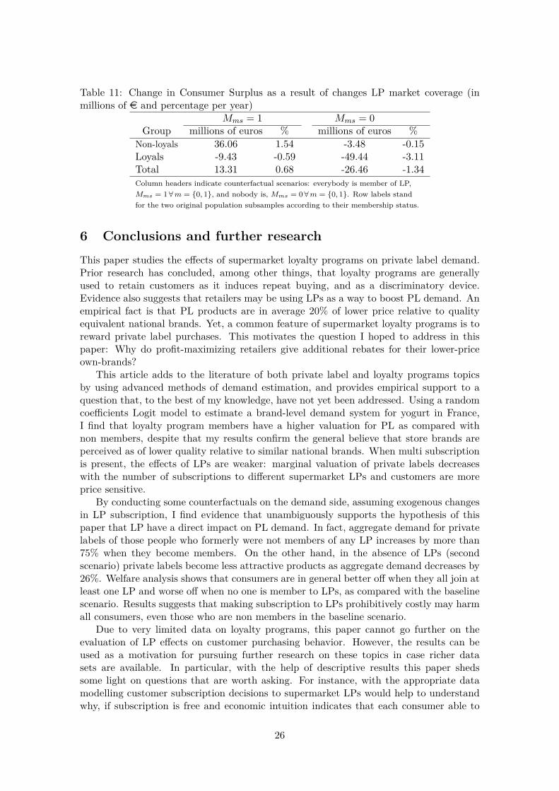
Table 11: Change in Consumer Surplus as a result of changes LP market coverage (inmillions of e and percentage per year)

Mms = 1 Mms = 0Group millions of euros % millions of euros %

Non-loyals 36.06 1.54 -3.48 -0.15Loyals -9.43 -0.59 -49.44 -3.11Total 13.31 0.68 -26.46 -1.34Column headers indicate counterfactual scenarios: everybody is member of LP,Mms = 1 ∀m = 0, 1, and nobody is, Mms = 0 ∀m = 0, 1. Row labels standfor the two original population subsamples according to their membership status.

6 Conclusions and further researchThis paper studies the effects of supermarket loyalty programs on private label demand.Prior research has concluded, among other things, that loyalty programs are generallyused to retain customers as it induces repeat buying, and as a discriminatory device.Evidence also suggests that retailers may be using LPs as a way to boost PL demand. Anempirical fact is that PL products are in average 20% of lower price relative to qualityequivalent national brands. Yet, a common feature of supermarket loyalty programs is toreward private label purchases. This motivates the question I hoped to address in thispaper: Why do profit-maximizing retailers give additional rebates for their lower-priceown-brands?

This article adds to the literature of both private label and loyalty programs topicsby using advanced methods of demand estimation, and provides empirical support to aquestion that, to the best of my knowledge, have not yet been addressed. Using a randomcoefficients Logit model to estimate a brand-level demand system for yogurt in France,I find that loyalty program members have a higher valuation for PL as compared withnon members, despite that my results confirm the general believe that store brands areperceived as of lower quality relative to similar national brands. When multi subscriptionis present, the effects of LPs are weaker: marginal valuation of private labels decreaseswith the number of subscriptions to different supermarket LPs and customers are moreprice sensitive.

By conducting some counterfactuals on the demand side, assuming exogenous changesin LP subscription, I find evidence that unambiguously supports the hypothesis of thispaper that LP have a direct impact on PL demand. In fact, aggregate demand for privatelabels of those people who formerly were not members of any LP increases by more than75% when they become members. On the other hand, in the absence of LPs (secondscenario) private labels become less attractive products as aggregate demand decreases by26%. Welfare analysis shows that consumers are in general better off when they all join atleast one LP and worse off when no one is member to LPs, as compared with the baselinescenario. Results suggests that making subscription to LPs prohibitively costly may harmall consumers, even those who are non members in the baseline scenario.

Due to very limited data on loyalty programs, this paper cannot go further on theevaluation of LP effects on customer purchasing behavior. However, the results can beused as a motivation for pursuing further research on these topics in case richer datasets are available. In particular, with the help of descriptive results this paper shedssome light on questions that are worth asking. For instance, with the appropriate datamodelling customer subscription decisions to supermarket LPs would help to understandwhy, if subscription is free and economic intuition indicates that each consumer able to

26

subscribe should do so, not everybody subscribes or, among those who subscribe, noteverybody does it to as many programs as available in the market. In fact, in France15% of customers are not members of any supermarket LP whatsoever and, among themembers, 20% are affiliated to only one supermarket. Another interesting question tobe explored is what are the effects of LPs on supermarket choice. This paper providessome descriptive results suggesting that members of a given supermarket loyalty programexpend in average a higher portion of their income in that supermarket compared to nonmember customers. I believe that in many cases supermarket choice comes first whenpeople need to go shopping, and brand choice comes next. In such cases LPs may playa key role in consumer’s decision, as they are supermarket-level rather than brand-levelmarketing devices.

Further research imply going deeper in the meaning of making customers loyal to astore or a particular brand and understanding the role played by loyalty programs in thiscontext. By adopting a measure of loyalty, such as the share of wallet or the shoppingintensity, it can be explored whether LPs are making customers loyal. A question thatremains to be answered is thus: are non members more loyal than members?

Finally, from a policy perspective this paper may be seen as a first step for assessingmore complex and interesting questions: Are loyalty programs being used by retailers as astrategy to strengthen their buyer power? Moreover, taking into account the theory resultthat loyalty programs allow retailers to increase PL prices, it is worth asking: Can loyaltyprograms be harmful for consumers at some point? Should policy authorities be cautiousabout the implementation of such marketing strategies? In order to answer such ques-tions a structural model of the supply side is needed, which should include the horizontal(competition among retailers with their own brands) as well as the vertical dimension(competition among retailers and manufacturers, i.e, PL against NB). A counterfactualexperiment on the supply side would allow to assess whether retailers are trying to exertsome buyer power or not, under the premise that retailers might use their bargainingpower to squeeze manufacturers’ margins. I hope to think further about this in the future.

27

Appendix

A A theoretical backgroundThis is a two-period model of oligopolistic competition with horizontal differentiation.38Consider two symmetric retailers (j = 1, 2) differentiated à la Hotelling and located at thetwo extremes of a line of length one. They supply the good at a constant marginal costc > 0 and compete for a mass of customers indexed by i ∈ [0, 1] uniformly distributedalong the Hotelling line. We assume unit demands, i.e., each consumer buys at most oneunit of the good in each period. Moreover, we assume the good is not storable.39

Consumer location xt is independently and identically distributed over time. In par-ticular, consumers cannot anticipate their second period location in period 1.40

At the beginning of the first period, retailers offer a loyalty program (LP) to consumersconsisting of a coupon B of a given amount of money determined by period 1 purchases andredeemable in period 2 in the same retailer’s stores. This rebate is given to a consumerconditional on his subscription to the retailer’s LP in the first period. We assume, forsimplicity, that consumers can only subscribe to one loyalty program and that the marketis fully covered, i.e., the utility of joining a LP is large enough so that it is better tosubscribe than the outside option.41Finally, we assume non-strategic forward-looking consumers with rational expectations.The structure of the model defines a two-stage game as follows:

• First stage: Retailers determine simultaneously first-period prices and loyalty rebatesto maximize their expected two-period profit function.

• Second stage: Prices, loyalty rebates and first-period market shares are realized.Each firm then decides her second-period price to maximize her second-period profittaking into account her subscribers and the eventual “non-loyal” customers (switch-ers) she could have in every period.

38In their 1990 paper R. Caminal and C. Matutes, who analyse the effects of alternative pricing policieson duopoly competition with endogenous switching costs, consider the commitment to a future rebatethrough a coupon as one of the pricing policies. The results coincide with those I obtain in this Sectionwith the difference that they derive the main results computationally whereas I solve for the equilibriumtariffs analytically. I hope this will provide a richer insight. In any case, this is not the main contributionof this paper and is intended to help mainly to derive objective economic intuition to frame the empiricalanalysis.

39Given the structure of the food retailing industry in which there are commonly more than two firms,one can argue that a circular city framework might better model this problem. However, for the purpose ofthis paper, where we try to explain consumer choice under the existence of loyalty rebates instead of a fullentry-location game, a linear city model with two differentiated retailers seems to be enough. Moreover,the empirical evidence shows that in average most people visit at most two different stores when they goshopping.

40Although this assumption is admittedly made for simplicity in order to introduce uncertainty in lo-cation and to avoid consumers anticipating second-period results from the first period, there are intuitiveinterpretations of it. We can think, for example, of a person who remembers running out of toothpastein the morning when going out of her workplace, and go to buy to the closest supermarket or on the wayhome; another example is that of a person having a craving for pizza after work and stops by to buy oneon the way home. We can also think of this assumption as uncertainty of tastes depending on the day orthe weather: maybe in a cold-rainy day I can feel like eating lasagna but in a sunny day I would prefereating salad or gazpacho instead.

41The subscription to a given LP does not imply that consumer has committed herself to repeat purchasesfrom the same retailer in the second period. As a consequence, consumers have always the choice to goto the retailer with the lower price given their second period location and the size of B, which becomes aswitching cost for those who decide to go to a different retailer.

28

We are looking for subgame-perfect equilibria.

Definition 1. The set of choices p∗11, B∗1 , p∗21 for firm 1 and p∗12, B

∗2 , p∗22 for firm 2 is

said to be a subgame-perfect equilibrium of the game if

• Second stage: For any given first-period prices and loyalty rebates p11, B1; p12, B2and for any given first-period market shares α1(p11, p12), α2(p11, p12), the pricesp∗21 and p∗22 constitute a Nash equilibrium.

• First stage: Given the second-period optimal prices p∗21, p∗22 and market shares

D1, D2, the quadruple p∗11, B∗1 ; p∗12, B

∗2 is a Nash equilibrium.

We are interested in the set of interior equilibria, therefore we impose an upper boundon Bj , which must be small enough so that the consumers’ demands remain interior:

0 ≤ Bj ≤ B

A.1 Second period

Let us assume p1j ,Bjj=1,2 as given. Moreover, let us assume that a mass αj ∈ (0, 1)of consumers subscribed to firm j’s loyalty program in the first period. The remaining(1 − αj) ≡ αk subscribed to rival’s LP. αj and αk denote, hence, firm j, k’s first-periodmarket share, respectively.

The utility of a consumer i located at x2 who has joined firm j’s LP is:

u− (p2j −Bj)− τx2 if he continues buying from retailer ju− p2k − τ(1− x2) if he switches to retailer k, ∀k = 1, 2

where u is consumer i’s valuation of the good and τ is a transportation cost parameterwhich is constant over time and symmetric across consumers.

Assuming that the consumer who is indifferent between the two retailers is located atx2 = Dj , firm j’s market share is defined by:

p2j −Bj + τDj = p2k + τ(1−Dj)

Solving for Dj yields firm j’s second-period market share:

Dj(p2j , p2k, Bj) = 12 + σ [p2k − (p2j −Bj)] , ∀j, k = 1, 2 (24)

where

σ ≡ 12τ (25)

is a parameter indicating the degree of substitutability between the two retailers.Firm j’s profit maximization problem writes as:

maxp2j

π2j = (p2j − c)(αjDj + (1− αj)Dk)− αjDjBj

FOC:

αjDj + (1− αj)Dk + (p2j − c)[αj∂Dj

∂p2j+ (1− αj)

∂Dk

∂p2j

]− αj

∂Dj

∂p2jBj = 0 (26)

29

Plugging ∂Dj

∂p2j= ∂Dk

∂p2j= −σ into (26) and solving for p2j yields:

p2j = c

2 + τ

2 + αjBj + p2k − (1− αj)Bk2 (27)

By the symmetry of the model, p2k has a similar expression to the previous equation.Plugging it to (27) and solving for p2j we have:

p∗2j(αj) = c+ τ + αjBj , ∀j = 1, 2 (28)

or

p∗21(α1) = c+ τ + α1B1 and p∗22(α2) = c+ τ + α2B2 (29)

Note that if we set Bj = 0, we get p = c+ τ which is the standard Hotelling price withunit demands.

A.2 First period

A consumer located at x1 will have the following instantaneous utility:

u− p1j − τx1 if he goes to retailer ju− p1k − τ(1− x1) if he goes to retailer k

Conditional on buying from retailer j in the first period, he will buy again in the secondperiod to this retailer if x2 satisfies:

x2 ≤ Dj ≡τ + p2k − p2j +Bj

2τThe consumer i’s expected second-period surplus is then:

δ

[∫ Dj

x=0(u− p2j +Bj − τx)dx+

∫ x=1

Dj

(u− p2k(αk)− τ(1− x))dx]

(30)

performing the integrals and rearranging, yields:

δ

(p2k − p2j +Bj + τ)Dj − τD2

j + u− p2k −τ

2

Hence, consumer i’s lifetime utility is:

u− p1j − τx1 + δ

(p2k − p2j +Bj + τ)Dj − τD2

j + u− p2k −τ

2

(31)

Similarly, conditional on buying from retailer k in the first period, the consumer con-tinues buying from her if:

x2 ≥ Dk ≡τ + p2k − p2j −Bk

2τThen, consumer i’s expected total surplus conditional on buying from k is:

u− p1k − τx1 + δ

(p2k − p2j −Bk + τ)Dk − τD2

k + u− p2k +Bk −τ

2

(32)

30

A consumer located at x1 = αj who is indifferent between retailers makes (32) = (31),which results in firm j’s market share:

αj = 12 + σ [(2p1k − δBk)− (2p1j − δBj)] (33)

where

σ ≡ τ

4τ2 + δ(Bj +Bk)2

is a ‘modified’ substitutability parameter that takes into account the dynamic effects ofLPs. Note that if we set Bj = Bk = 0, we obtain the standard market share in the staticHotelling model.

Equation (33) tells us that even though the consumer does not receive an immediaterebate, he perceives current prices lower as if the loyalty discount were immediate. Also,that a delayed rebate does not have the same impact on the demand as an immediate oneas long as the discount factor reduces the impact of this loyalty rebate, stimulating onlya fraction of demand increase per unit of price reduction.

Assuming that firms discount the future at the same rate δ as consumers, firm j’soverall profit function is given by:

Πj = π1j(p1j , p1k) + δπ2j (αj(p1j , p1k, Bj , Bk)) (34)

where:

π1j = (p1j − c)αj(p1j , p1k, Bj , Bk)

= (p1j − c)(1

2 + σ [(2p1k − δBk)− (2p1j − δBj)])

(35)

and

π2j = (p2j − c)(αjDj + (1− αj)Dk)− αjDjBj

= τ2 − αj(1− αj)(Bj +Bk)Bj2τ (36)

Firm j’s problem is then:maxp1j ,Bj

Πj

FOCs:

∂Πj

∂p1j= 1

4τ2 + δ(Bj +Bk)2

[2τ(p1k − 2p1j + τ + δ

(Bj −Bk)2 + c

)+ δ

(Bj +Bk)2

2

]

+ δ

2τ

[(Bj +Bk)Bj

∂αj∂p1j

(−(1− αj) + αj)]

= 0

In a symmetric equilibrium, p1j = p1k = p∗1, αj = 1/2, Bj = Bk = B:

p∗1 = c+ τ + δB2

τ, (37)

p∗2 = c+ τ + B

2 (38)

31

And the respective profits are:

π∗1 = 14σ + δσB2 π∗2 = 1

4σ −σB2

2 (39)

Π∗ = (1 + δ) 14σ + δ

σB2

2 (40)

Where σ is the standard substitutability parameter as defined in (25). Note that ifwe set B = 0 we get π1 = π2 = 1

4σ , which is the Hotelling profit in a model with unitdemands.

As shown in the previous equations, retailers’ instantaneous profits can be some periodshigher and some others lower than those they would obtain in absence of LPs. However,overall profits are higher thanks to the rise in prices induced by LPs. According to equation(40), overall profits increase in the loyalty rebate. Given the transportation costs, thehigher the B the better for the retailer.

B First-stage resultsIn this Section I present the regressions conducted as a first step to obtain predicted price,membership and the deltas necessary to compute the optimal instruments.

B.1 Modelling prices

As pointed out previously, I assume that the price of a particular brand in a department isa linear function of brand and supermarkets characteristics and the average prices of thesame brand in all the regions of the country (excluding the department from the averageprice of the region the market is located in). These prices are used as proxies of marginalcosts under the assumption that a supermarket chain has some common marginal costs inall its stores across the country, and then retail prices contain information on that commoncosts (see Section 4 for more details).

Table B.1 displays the results of the linear regression of the price of the brand variety jin supermarket s at t on average prices of the same brand in the 21 administrative regionsof France, and brand dummy variables and week dummy variables as controls. The factthat all the estimates are significant at 1% level and the high R-squared suggest that priceshave important explanatory power.

B.2 Modelling the membership decision

As explained before, the information I have about loyalty programs is very limited: adummy variable indicating whether a given household was member of the loyalty programof the supermarket it purchased from in 2006 is all I have. We do not know anythingabout how long ago the household is member of it, nor if the household gets the promisedcoupons or even if it redeems them.

Due to these data limitations, I cannot fully explain the determinants of the indi-vidual decision to subscribe to a loyalty program. Ideally, a proper way to identify theparameters for the subscription decision modelling is having observations on demograph-ics, the purchasing behaviour of the households, and loyalty programs’ and supermarkets’characteristics including the reward system, before and after the subscription decision ismade.

32

Table B.1: Results from a linear regression for priceEst. s.e.

pR1 -0.632 0.132pR2 -2.902 0.194pR3 -1.218 0.227pR4 -1.546 0.148pR5 -1.591 0.100pR6 -2.717 0.194pR7 -2.820 0.288pR8 -1.915 0.216pR9 -1.940 0.170pR10 -0.895 0.140pR11 -6.149 0.276pR12 -2.236 0.191pR13 -0.863 0.164pR14 -2.346 0.167pR15 -3.253 0.212pR16 -1.008 0.135pR17 -1.660 0.117pR18 -1.233 0.139pR19 -1.310 0.174pR20 -2.881 0.283pR21 -6.385 0.338adj. R2 0.840Based on 37,662 observations.Robust s.e. in parentheses.Regressions include brandand time dummy variables.

What I can do, nevertheless, is exploiting the data I have to give a clue of how loyaltyprogram characteristics and demographics are correlated with the membership status of ahousehold to a supermarket LP. In addition, this exercise allows me to find instruments totreat the endogeneity of the loyalty membership indicator caused by its correlation withdepartment-week specific deviation from the overall mean valuation of the supermarketcharacteristics (∆ξst).

I collected some data on the characteristics of each loyalty program that do not vary bymarket, namely, a dummy variable equal to one if the program includes both NB and PLin the reward system and zero otherwise, a dummy variable equal to one if the customercan either subscribe to the program by Internet or at least download the inscription formand zero otherwise, the average rebate in euros per 100 e expended in the supermarket,and dummies for whether the program has an upper bound for accumulating rebates(Cap), a threshold to be able to redeem certain amount of points or money accumulated(Threshold) and a variable equal to the number of months for the card to expire in caseof lack of use (Expire_date).42

From the data set described in section 3.1, I used demographic variables as householdsize, income, a dummy equal to one if the household has at least one car, age of the head

42To obtain this information, I reviewed carefully each supermarket program’s “Terms and Conditions”document and identify some common categories describing the general structure of the programs. Thesedocuments were obtained from each supermarket website in 2011 and 2012. Although the information isused to instrument a decision that could have been taken even before 2006 (the year of the homescan database used in this article), all the programs where launched before 2006 and I believe the structure has notchanged a lot since then.

33

of household and a dummy equal to one if the family lives in urban areas. In addition,I constructed variables such as the number of different stores visited by the householdmembers within a week, the number of shopping trips to a same retailer in a month andthe number of members to the LP of a given supermarket in the rest of the country(excluding the department where the household was located).

Table B.2 displays the results of OLS and Logit regressions of the dummy variableindicating household membership to a supermarket loyalty program on the variables pre-viously described. After a first specification with all the covariates, the LP characteristicsCap, Threshold and Expire_date were either non significant at 5% level or had a differentsign than expected or both. Thus, I excluded them form the final specification displayedin the table.

Table B.2: Results from OLS and Logit regressions for LP membershipVariable OLS Logit

LPs characteristicsLog total Sup. LP members 0.141∗∗ 0.892∗∗

excluding location depart. (0.028) (0.185)NB included 0.0499∗∗ 0.322∗∗

(0.020) (0.137)Online access to inscription 0.0410∗∗ 0.261∗∗

form (0.012) (0.074)Log of average reward per 0.0110∗∗ 0.0692∗∗

100 espent (0.005) (0.033)Demographics# of different stores −0.272∗∗ −1.643∗∗

visited a week (0.044) (0.235)# trips to the same 0.156∗∗ 1.127∗∗

retailer per month (0.011) (0.093)Household size 0.0288∗∗ 0.190∗∗

(0.003) (0.023)Log income -0.0132 −0.0928∗

(0.009) (0.057)Log age 0.0365∗∗ 0.221∗∗

(0.015) (0.088)Car 0.0683∗∗ 0.369∗∗

(0.022) (0.114)Lives in city 0.00869 0.0615

(0.009) (0.058)Constant −0.632∗∗ −7.515∗∗

(0.254) (1.660)N 9,976 9,976R2 0.035adj. R2 0.034Robust standard errors in parentheses.∗∗ Significant at 5% and ∗ at 10% level.

Although we cannot say that this variables explain the whole variation of the dependentvariable, and this is confirmed by the low adjusted R2, the results are quite appealing. Onthe one hand, in the Logit regression (column 2) all the parameters are significant, andon the other hand, the signs of the variables are according to the intuition.

In the first place, the probability for a customer to join supermarket j loyalty programincreases with the number of members in the rest of the country, which means that themore popular the program is, the more attractive is for a customer to join most probably

34

because this is a signal of the program quality. Moreover, this probability also increaseswith household characteristics such as the number of trips the household members do tothe retailer j, being an indicator of shopping intensity, the more often a customer goes tothe same store, the more informed about prices and promotions she is and, consequently,the more likely to benefit from rebates; household size, age, car ownership and living inurban areas which facilitates the access to the retailer.

Second, individual characteristics such as the income and the multi-store shoppingbehavior make consumers to be less interested in joining LPs because either they are lesssensitive to small price cuts or they are less likely to get rewards. In fact, one can expectthat as income increases supermarket loyalty programs become less attractive becausewealthier people may be less sensitive to little price cuts and also because loyalty re-bates are generally addressed to middle quality goods rather than to high quality brandedproducts. Regarding the multi-store shopping behavior, it is more difficult to accumulatepoints or money in a loyalty account when purchases are not concentrated in one retailer,which makes individuals with this shopping profile either less interested to join any loyaltyprogram or willing to join all of them, but not likely to use them as rewards will never beattainable.

As for the the LP characteristics included in the regression: Logit results show thatthe probability of joining a LP increases with the fact that both NB and PL purchases givethe customers points to get a future rebate compared to those programs including onlyPL, also with the possibility of joining the program online (or at least having access tothe inscription form) and the average reward in euros, i.e, the better rewarding programsare the more likely to attract customers to their loyalty program.

B.3 First-stage estimation of the full model

The results of the first-stage estimation of the full model using the set of inefficient in-struments for the endogenous variables are basically of the expected sign. However, mostestimates are statistically non significant due to the very large robust standard errorsobtained. In addition, some convergence problems were experienced as the size of theestimates and in some cases the sign were quite sensitive to the provided set of startingvalues. All this suggests that the instruments used to identify the parameters of the fullmodel are not performing well, even though they are similar to the instruments used insome standard papers. This may be due to the fact that they are just helping to identifythe parameters in the linear part of the model (θ1) and not those of the whole model(θ1, θ2). This fact empirically supports the need to use optimal instruments as the bestway to overcome endogeneity problems in this kind of models.

B.4 Own- and cross-price elasticities

Table B.4 presents the estimated own- and cross- price elasticities for the leading 12 brandvarieties based on their national market shares. The columns in the table indicate de pricesand the rows the market shares used to compute the variation, so that for instance, theentry located in row 2 column one gives the elasticity of brand 2 with respect to a changein the price of brand 1.

One of the advantages of a random-coefficients model, as it was said previously, is thatit gives more realistic substitution patterns allowing for different brands to have differentvalues for the elasticity due to the change in the price of a given price, as opposed tothe simple Logit where all the elasticities in the same column would have the same cross-price elasticities. As a consequence, estimated elasticities vary by brand and by market.

35

Table B.3: First-stage results from the Mixed Logit model with inefficient instrumentsaMeans Std. Deviations Interactions with Demographic variables

Variable (β’s) (σ’s) HH size Income # SubscriptionsConstantb -3.631 1.353 -0.967 0.922

(1.388) (1.865) (13.454) (4.787)Price -6.399 2.301 -1.748 0.764 1.331

(5.253) (6.090) (12.456) (25.647) (14.523)LP member (Mms) -8.338 6.223 -0.967

(6.896) (2.246) (9.011)PL dummyb -2.634 2.755 -1.331 0.764 -7.803

(2.270) (3.569) (4.305) (4.120) (5.237)LP member×PL dummy 7.935 4.347

(3.381) (3.344)Plasticb -0.035 2.114

(0.483) (1.266)Sugarb -0.223 0.562

(0.240) (4.803)Wholemilkb -2.998 0.670

(1.035) (3.779)GMM Objective 1,045MD χ2 4139681a Based on 37,662 observations. Except where noted, parameters were estimated using GMM. All regressionsinclude brand and week dummies. Asymptotically robust s.e. are given in parentheses.b Estimated using a minimum-distance procedure.

In order to give an idea of the estimated substitution patterns, Table B.4 presents themedians of the own- and cross-price elasticities over the 7,704 in the sample. The medianelasticities of the outside good with respect to column brand prices are also displayed.

36

TableB.4:

Med

ianow

n-an

dcross-priceelastic

itiesa

Brand

b1b3

b7b8

b9b1

1b1

2b1

5b1

6b1

8b2

1b2

3b2

4b2

8b2

9P

L 1-2.612

0.017

0.006

0.004

0.005

0.006

0.010

0.000

0.001

0.000

0.000

0.000

0.001

0.000

0.000

20.033

0.262

0.159

0.119

0.121

0.162

0.180

0.004

0.031

0.002

0.002

0.005

0.027

0.013

0.003

30.009

-15.995

0.045

0.029

0.022

0.032

0.035

0.001

0.007

0.000

0.000

0.002

0.008

0.003

0.001

40.030

0.269

0.125

0.081

0.081

0.119

0.163

0.002

0.027

0.001

0.001

0.006

0.025

0.009

0.002

50.041

0.387

0.271

0.144

0.148

0.239

0.244

0.006

0.043

0.003

0.003

0.009

0.050

0.016

0.005

60.009

0.157

0.053

0.035

0.036

0.061

0.049

0.001

0.011

0.001

0.000

0.002

0.009

0.003

0.001

70.005

0.052

-8.893

0.018

0.017

0.022

0.019

0.001

0.004

0.000

0.000

0.001

0.004

0.002

0.000

80.004

0.040

0.019

-7.310

0.012

0.017

0.021

0.000

0.003

0.000

0.000

0.001

0.004

0.002

0.000

90.003

0.023

0.016

0.007

-4.777

0.012

0.011

0.000

0.002

0.000

0.000

0.001

0.003

0.001

0.000

100.015

0.091

0.053

0.037

0.037

0.040

0.044

0.002

0.010

0.001

0.000

0.002

0.010

0.004

0.001

110.005

0.040

0.022

0.015

0.014

-10.365

0.027

0.001

0.004

0.000

0.000

0.001

0.004

0.002

0.000

120.009

0.049

0.031

0.017

0.020

0.031

-12.624

0.001

0.008

0.000

0.000

0.002

0.009

0.003

0.001

NB 13

0.008

0.100

0.038

0.027

0.027

0.039

0.047

0.003

0.028

0.002

0.001

0.005

0.030

0.011

0.003

140.005

0.047

0.037

0.015

0.016

0.024

0.047

0.003

0.024

0.001

0.001

0.005

0.026

0.008

0.002

150.000

0.002

0.001

0.001

0.001

0.001

0.002

-1.834

0.001

0.000

0.000

0.000

0.001

0.000

0.000

160.001

0.012

0.007

0.004

0.004

0.005

0.009

0.001

-11.919

0.000

0.000

0.001

0.004

0.002

0.000

170.002

0.020

0.009

0.007

0.008

0.012

0.016

0.001

0.009

0.001

0.000

0.001

0.008

0.005

0.001

180.000

0.000

0.000

0.000

0.000

0.000

0.000

0.000

0.000

-0.837

0.000

0.000

0.000

0.000

0.000

190.010

0.072

0.048

0.025

0.031

0.038

0.089

0.004

0.028

0.003

0.001

0.007

0.025

0.016

0.003

200.009

0.142

0.057

0.028

0.020

0.050

0.044

0.005

0.034

0.004

0.002

0.009

0.033

0.011

0.003

210.000

0.000

0.000

0.000

0.000

0.000

0.000

0.000

0.000

0.000

-0.491

0.000

0.000

0.000

0.000

220.001

0.016

0.005

0.004

0.005

0.005

0.002

0.000

0.003

0.000

0.000

0.001

0.003

0.001

0.000

230.000

0.002

0.001

0.001

0.001

0.001

0.001

0.000

0.001

0.000

0.000

-2.694

0.001

0.000

0.000

240.001

0.007

0.003

0.003

0.003

0.003

0.006

0.000

0.002

0.000

0.000

0.001

-10.906

0.001

0.000

250.006

0.056

0.024

0.021

0.017

0.030

0.037

0.003

0.018

0.001

0.001

0.005

0.017

0.009

0.002

260.000

0.000

0.000

0.000

0.000

0.000

0.000

0.000

0.000

0.000

0.000

0.000

0.000

0.000

0.000

270.022

0.169

0.091

0.061

0.070

0.080

0.150

0.009

0.070

0.003

0.003

0.015

0.048

0.031

0.006

280.000

0.002

0.001

0.001

0.001

0.001

0.002

0.000

0.001

0.000

0.000

0.000

0.001

-4.371

0.000

290.000

0.001

0.000

0.000

0.000

0.000

0.000

0.000

0.000

0.000

0.000

0.000

0.000

0.000

-0.852

300.004

0.047

0.026

0.015

0.014

0.022

0.025

0.002

0.019

0.001

0.001

0.003

0.018

0.007

0.002

310.003

0.025

0.012

0.010

0.008

0.014

0.016

0.002

0.009

0.001

0.000

0.002

0.009

0.004

0.001

aEachof

theentriescorrespo

ndto

themedianof

theelasticities

from

the7,704markets.Theygive

thepe

rcentchan

gein

marketshareof

agivenbran

dwithaon

epe

rcentvariationin

either

own-price(for

thosein

themaindiagon

al)or

thepriceof

anotherbran

d(for

thoseou

tsidethemaindiagon

al).

Intheho

rizontal

axis

thebran

dswiththelargestmarketshares

aredisplayed.

The

fullmatrixis

availableon

deman

d.bCorrespon

dsto

theou

tsidego

od.

37

References

1. Amemiya, Takeshi (1974), “The nonlinear Two-Stage Least Squares Estimator”,Journal of Econometrics, No. 2, pp. 105-110.

2. (1977), “The maximum likelihood and the nonlinear three-stage leastsquares estimator in the general nonlinear simultaneous equation model”, Econo-metrica, Vol. 45, No. 4, pp. 955-968.

3. Bierlaire, Michel, Bolduc, Denis and McFadden, Daniel (2008), “The estimationof Generalized Extreme Value models from choice-based samples”, TransportationResearch Part B: Methodological, vol. 42, No.. 4, pp. 381-394.

4. Berges-Sennou Fabian, Bontems Phillip and Requillart V. (2009), “L’impact économiquedu développement des marques de distributeurs”, Working paper, Toulouse Schoolof Economics, 30 p.

5. Berges-Sennou, Fabian (2006), “Store loyalty, bargaining power and the private labelproduction issue”, European Review of Agricultural Economics, Vol. 33, No. 3, pp.315-335.

6. Berry, Steven (1994), “Estimating discrete-choice models of product differentiation”,The RAND Journal of Economics, Vol. 25, No. 2, pp. 242-262.

7. Berry, Steven, Levinsohn, James and Pakes, Ariel (1995), “Automobile prices inmarket equilibrium”, Econometrica, Vol. 63, No. 4, pp. 841-890.

8. (1999), “Voluntary export restraints on automobiles: evaluating a tradepolicy”, The American Economic Review, Vol. 89, No. 3, pp. 400-430.

9. Bolton, R., Kannan, P. and Bramlett, M. (2000), “Implications of loyalty programmembership and service experiences for customer retention and value”, Journal ofthe Academy of Marketing Science, Vol. 28, No. 1, pp. 95-108.

10. Bonnet, Céline and Dubois Pierre (2010), “Inference on vertical contracts betweenmanufacturers and retailers allowing for nonlinear pricing and resale price mainte-nance”, The RAND Journal of Economics, Vol. 41, No. 1, pp. 139-164.

11. Caillaud, Bernard and De Nijs, Romain (2011), “Strategic loyalty reward in dynamicprice discrimination”, Paris School of Economics Working Papers, No. 2011-29, 38p.

12. Caminal, Ramon and Matutes, Carmen (1990), “Endogenous switching costs in aduopoly model”, International Journal of Industrial Organization, Vol. 8, No. 3,pp. 353-373.

13. Chamberlain, Gary (1987), “Asymptotic efficiency in estimation with conditionalmoment restrictions”, Journal of Econometrics, No. 34, pp. 305-334.

14. Chen, Yongmin and Pearcy, Jason (2010), “Dynamic pricing: when to entice brandswitching and when to reward consumer loyalty”, The RAND Journal of Economics,Vol. 41, No. 4, pp. 674-685.

38

15. Chintagunta, Pradeep, Bonfrer, André and Song, Inseong (2002), “Investigatingthe effects of store-brand introduction on retailer demand and pricing behavior”,Management Science, Vol. 48, No. 10, pp. 1242-1267.

16. Cremer, Jacques (1984), “On the economics of repeat buying”, The RAND Journalof Economics, Vol. 15, No. 3, pp. 396-403.

17. European Commission (2011), “The impact of private labels on the competitivenessof the European food supply chain”, available at:http : //ec.europa.eu/enterprise/sectors/food/documents/studies/commentsprivlaben.htm

18. Dubé, Jean-Paul, Fox, Jeremy and Su, Che-Lin (2012), “Improving the numericalperformance of BLP static and dynamic aggregate discrete choice random coefficientsdemand estimation”, Econometrica, Vol. 80, No. 5, pp. 2231-2267.

19. Fudenberg, Drew and Tirole, Jean (2000), “Customer poaching and brand switch-ing”, The RAND Journal of Economics, Vol. 31, No. 4, pp. 634-657.

20. Hausman, Jerry (1996), “Valuation of new goods under perfect and imperfect com-petitio”, The Economics of New Goods, Studies in Income and Wealth, Vol. 58, ed.by T. Bresnahan and R. Gordon, National Bueau of Economic Research, Chicago.

21. Jorgenson, Dale and Laffont, Jean-Jacques (1974), “Efficient estimation of nonlinearsimultaneous equations with additive disturbances”, Annals of Economic and SocialMeasurement, 3/4, pp. 615-640.

22. Kelejian, Harry (1971), “Two-stage least squares and econometric systems linear inparameters but nonlinear in endogenous variables”, Journal of the American Eco-nomic Association, Vol. 66, No. 334, pp. 373-374.

23. Klemperer Paul (1987a), “Markets with consumer switching costs”, The QuarterlyJournal of Economics, Vol. 102, No. 2, pp. 375-394.

24. (1987b), “The competitiveness of markets with switching costs”, The RANDJournal of Economics, Vol. 18, No. 1, pp. 138-150.

25. Knittel, Christopher and Metaxoglou, Konstantinos (2012), “Estimation of randomcoefficient demand models: two empiricists’ perspective”, non-published manuscript.

26. Lewis, Michel (2004), “The influence of loyalty programs and short-term promotionson customer retention”, Journal of Marketing Research, Vol. 41, pp. 281-292.

27. Lal, Rajiv and Bell, David (2003), “The impact on frequent shopper programs ingrocery retailing”, Quantitative Marketing and Economics, No. 1, pp. 179-202.

28. Lederman, Mara (2007), “Do enhancements to loyalty programs affect demand? Theimpact of international frequent flyer partnerships on domestic airline demand”,RAND Journal of Economics, Vol. 38, No. 4, pp. 1134-1158.

29. Manski, Charles and Lerman, Steven (1977), “The estimation of choice probabilitiesfrom choice based samples”, Econometrica, Vol. 45, No. 8, pp. 1977-1988.

30. McFadden, Daniel (1999), “Computing willingness-to-pay in random utility models”,in J. Moore, R. Riezman, and J. Melvin, eds., Trade, Theory and Econometrics:Essays in Honour of John S. Chipman, Routledge, London, pp. 253?274.

39

31. Nasser, Sherif, Turcic, Danko and Narisimhan, Chakravarthi (2013), “National Brand’sResponse to Store Brands: Throw In the Towel or Fight Back?”, Marketing Science,Vol. 32, No. 4, pp. 591-608.

32. Nevo, Aviv (2000a), “A practitioner’s guide to estimation of random-coefficientsLogit models of demand”, Journal of Economics and Management Strategy, Vol. 9,No. 4, pp. 513-548.

33. (2000b), “Mergers with differentiated products: the case of the ready-to-eatcereal industry”, RAND Journal of Economics, Vol. 31, No. 3, pp. 395-421.

34. (2001), “Measuring market power in the ready-to-eat cereal industry”,Econometrica, Vol. 69, No. 2, pp. 307-342.

35. Nevo, Aviv and Wolfram, Catherine (2002), “Why do manufacturers issue coupons?An empirical analysis of breakfast cereals”, RAND Journal of Economics, Vol. 33,No. 2, pp. 319-339.

36. Newey, Whitney (1990), “Efficient instrumental variables estimation of nonlinearmodels”, Econometrica, Vol. 58, No. 4, pp. 809-837.

37. Raju, Jagmohan, Sethuraman, Raj and Dhar, Sanjay (1995), “The introduction andperformance of store brands”, Management Science, Vol. 41, No. 6, pp. 957-978.

38. Reynaert, Mathias and Verboven, Frank (2013), “Improving the performance of therandom coefficients demand models: the role of optimal instruments”, unpublishedWorking paper.

39. Steenkamp, Jan-Benedict and Geyskens, Inge (2013), “Manufacturer and RetailerStrategies to Impact Store Brand Share: Global Integration, Local Adaptation, andWorldwide Learning”, Marketing Science, forthcoming.

40. Soberman, David and Parker, Phillip (2006), “The economics of quality-equivalentstore brands”, International Journal of Research in Marketing, No. 23, pp. 125-139.

41. Train, Kenneth (2009), Discrete Choice Methods with Simulation, Second edition,Cambridge University Press.

42. Wooldrige, Jeffrey (2002), Econometric Analysis of Cross Section and Panel Data,The MIT Press.

40