Embed Size (px)
Citation preview

1
Advanced Finite Element
Title: The Geometric Nonlinear Analysis of Iso-P
Quadrilateral Element in 2D
Professor: Carlos Felippa
Student: Mohammadreza Mostafa
PHD student in CVEN Dept
Spring 2009

2
1-Goals:
Solid elements can be widely used in many engineering problems. They reason is that solid
elements can model the behavior of various structures such as structural elements in civil
engineering (beams and columns) and continuum media in 2D and 3D ( slabs, walls, thick and
thin plates and etc..). On the other hand, since the solid element has only translational degrees of
freedom, it is very easily formulated and implemented in finite element frames. For example, the
shell element which has out of plane bending has rotational degree of freedom that is much
complicated in nonlinear formulations.
It is noticeable that the solid element is more expensive than the other elements with rotational
degrees of freedom due to the number of elements required to model the geometry of the
structure of interest.
The afore-mentioned application of solids is a motivation to develop a general FEM code to
model the geometric nonlinear behavior of solid element.
The goal of this term project is to perform the Geometric Nonlinear Analysis of Iso-P
Quadrilateral Element in 2D. In order to get to this goal the followings are presented in this
project: 1. A tour of geometric nonlinear finite element
2. The formulation of 4-node quadrilateral Iso-parametric element
3. Explanation of The FEM code (assumptions, capabilities of the code)
4. Verification of the code by some examples and comparison with analytical
solutions
5. Presentation of some special cases and interpretation of the results
6. Conclusions and further researches
7. Appendix A, the code

3
2-Tour of Geometric Nonlinear Finite Element
2-1-Sources of nonlinearity:
2-1-1-Geometric Nonlinearity
Physical source
Change in geometry as the structure deforms is taken into account in setting up the strain
displacement and equilibrium equations.
Applications:
Slender structures in aerospace, civil and mechanical engineering applications. (Tensile
structures such as cables and inflatable membranes, metal and plastic forming and stability
analysis of all types)
Mathematical source
Strain-displacement equations:
e = Du
The operator D is nonlinear when finite strains (as opposed to infinitesimal strains) are expressed
in terms of displacements. Internal equilibrium equations:
b= -D*σ
In the classical linear theory of elasticity, D* = DT is the formal adjoint of D, but that is not
necessarily true if geometric nonlinearities are considered.
2-1-2-Material Nonlinearity
Physical source
Material behavior depends on current deformation state and possibly past history of the
deformation. Other constitutive variables (prestress, temperature, time, moisture, electromagnetic
fields, etc.) may be involved.

4
Applications
Structures undergoing nonlinear elasticity, plasticity, viscoelasticity, creep, or inelastic rate
effects
Mathematical source
The constitutive equation that relates stresses and strains is the same as that of a linear elastic
material
σ = E e
where the matrix E contains elastic modulus. If the material does not fit the elastic model,
generalizations of this equation are necessary, and a whole branch of continuum mechanics is
devoted to the formulation, study and validation of constitutive equations.
2-1-3-Force BC Nonlinearity
Physical Source
Applied forces depend on deformation.
Applications
The most important engineering application concerns pressure loads of fluids. These include
hydrostatic loads on submerged or container structures; aerodynamic and hydrodynamic loads
caused by the motion of aeriform and hydroform fluids (wind loads, wave loads, and drag
forces). Of more mathematical interest are gyroscopic and non-conservative follower forces, but
these are of interest only in a limited class of problems, particularly in aerospace engineering.
Mathematical source
The applied forces (prescribed surface tractions t and/or body forces b) depend on the
displacements:
t �t(u), b ��b(u)
The former is more important in practice.

5
2-1-4-Displacement BC Nonlinearity
Physical source
Displacement boundary conditions depend on the deformation of the structure.
Applications
The most important application is the contact problem, in which no-interpenetration conditions
are enforced on flexible bodies while the extent of the contact area is unknown. Non-structural
applications of this problem pertain to the more general class of free boundary problems, for
example: ice melting, phase changes, flow in porous media. The determination of the essential
boundary conditions is a key part of the solution process.
Mathematical source
For the contact problem: prescribed displacements d depend on internal displacements u:
d �d(u)
More complicated dependencies can occur in the free-boundary problems mentioned above.
2-1-5-Sources of Nonlinearity and Tonti diagram
As it is seen in the diagram, the Geometric nonlinearity affects the balance equation and
kinematic equation while the material nonlinearity affects the constitutive equation.
The force boundary condition and displacement boundary condition nonlinearities affect the
force boundary conditions and displacement boundary condition links respectively.

6
2-2-Nonlinear analysis formulation:
2-2-1-Force Residual vector:
In all the static geometric nonlinear problems we solve the following equation which is called the
“force residual”. ���� �� � �
This vector includes all the discrete equilibrium equations encountered in nonlinear static
structural analysis formulated by the displacement method.
Here u is the state vector containing the unrestrained degrees of freedom that characterize the
configuration of the structure, r is the residual vector that contains out-of-balance forces
conjugate to u, and Λ is an array of assignable control parameters.
In structural mechanics, control parameters are commonly mechanical load levels. They may
also be, however, prescribed physical or generalized displacements, temperature variations,
imperfection amplitudes and even (in design and optimization) geometric dimensions or material
properties. The degrees of freedom collected in u are usually physical or generalized unknown
displacements.
In conservative systems, r is the gradient of the total potential energy Π(u ,Λ) for fixed Λ as
below:
� � �� An alternative version of above equation that displays more physical meaning is the force-
balance form: ���� � ��� �� In this form p denotes the configuration-dependent internal forces resisted by the structure
whereas f are the control-dependent external or applied forces, which may also be configuration
dependent.
The residual r is either r ��p ��f or r ��f ��p, the two versions being equivalent except for sign.
The force equilibrium equations r ��0 or f ��p express the fact that the total potential energy is
stationary with respect to variations of the state vector when the structure is in static
equilibrium.

7
If a total potential energy exists, the decomposition becomes:
� � �� �������� � ��
Where U and P are the internal and external energy components, respectively, of � � � � �
2-2-2-Stiffness and Control Matrix:
Varying the vector r with respect to the components of u while keeping Λ fixed yields the
Jacobian matrix K:
�� � ��� This is called the tangent stiffness matrix in structural mechanics applications. The inverse of K,
if it exists, is denoted by�� � ����; a notation suggested by the name flexibility matrix used in
linear structural analysis for the reciprocal of the stiffness. If r derives from a potential, both K
and F are symmetric matrices.
Varying the negative of r with respect to Λ while keeping u fixed yields the control matrix as
below:
�� � � ��� 2-2-3-Staging:
Multiple control parameters are quite common in real-life nonlinear problems. They are the
analog of multiple load conditions in linear problems. But in the linear world, multiple load
conditions can be processed independently because any load combination is readily handled by
superposition. In nonlinear problems, however, control parameters are not varied independently.
It means that we cannot superpose the effect of each load case on the structure.
As an example, consider a bridge which has different load cases such as dead, live, earthquake,
wind, temperature changes and foundation settlement. There are six control parameters
corresponding to each of load cases. � � ���� ��� � � ��� In reference configuration the Λ is the vector of zeros. � !" � ������������� Suppose the Λ is Λ1 for dead load and Λ4 for earthquake:

8
�� � �# � ��$������������������% � ������� �&����� In order to get from � !" to �# we do the first staging (���. Then in order to get from �# to
�%we do the following stage:
�� � ��$����� �&����� The other load cases are involved in the staging as the above procedure.
2-2-4-One parameter residual:
From this section on we reduce the number of stages to one, because the problem that we are
planning to solve has only one load case. Hence, the load control parameter vector has only one
component, so we only have Λ={λ}. The residual vector becomes as follows: ���� '� � �
The corresponding residual-derivative equations are:
�( � ��( � )'( * � �� ���������) � � �'
Where K is the tangent stiffness matrix and q is the incremental load vector. + � ���)
This vector is called the incremental velocity vector and is an important component of all
methods.
2-2-5-Separable Residuals and Proportional Loading
The force-balance equivalent for a one-parameter residual equation is: ���� � ��� '� If the right hand side, which represents the external force vector, does not depend on the state
parameters u, the system is called separable. So: ���� � �'� Furthermore, if f is linear in λ the loading is said to be proportional. Obviously q ��∂f/∂λ is then
a constant vector.

9
2-3-Critical points (Limit and Bifurcation point):
It is assumed that the structural system is conservative and consequently K is symmetric.
Response points at which K becomes singular are of great interest in the applications because of
their intimate connection to structural stability. These are called critical points, and also
nonregular or singular points. At these points the velocity vector v is not uniquely determined by
q. This means that the structural behavior cannot be controlled by the parameter λ.
It is convenient to distinguish the following types of critical points:
1. Isolated limit points, at which the tangent to the equilibrium path is unique but normal to
the λ axis so V becomes infinitely large.
2. Multiple limit points, at which there the tangent lies in the null space of K and is not
unique but still normal to the λ axis.
3. Isolated bifurcation points also called branch points or branching points, from which two
equilibrium path branches emanate and so there is no unique tangent. The rank deficiency
of K is one.
4. Multiple bifurcation points, from which more than two equilibrium path branches
emanate. The rank deficiency of K is two or greater.
To classify critical points we proceed as follows. Let z be a null right eigenvector of K at a
critical point, that is: �, � �
Since K is assumed symmetric�,-� � �; that is, z is also a left null eigenvector. The parametric
differential equation of the equilibrium path is ./( �� �0�'( which multiplied through by dt
becomes: �1� � )1'
Premultiply both sides by 2- and use 2-� � � to get: 2-)1' � �
Two cases exist:
• Case 1 2-) 3 �
Then dλ must vanish, and we have a limit point. The point is isolated if z is the only null
eigenvector and multiple otherwise.

10
• Case 2 2-) � �
Then we have a bifurcation or branching point. The point is isolated if z is the only null
eigenvector and multiple otherwise. The key physical characteristic of a bifurcation point is an
abrupt transition from one deformation mode to another mode.
The following figures illustrate isolated limit points (identified as L1, L2, ...) and bifurcation
points (identified as B1, B2, . . .):
Limit points L1 and L2 and bifurcation point (B) for a two degree of freedom
System (u1, u2) shown on the u1 versus λ plane. Limit point (“snap through” behavior) occurs before bifurcation. Full lines represent physically “preferred” paths.
In this picture the bifurcation point B1 implying “buckling” behavior occurs before the limit point L1, which is physically unreachable.

11
The equilibrium path is shown in the 3D space (u1, u2, λ). This is the type of response exhibited
by a uniformly pressurized deep arch, for which u1 and u2 are amplitudes of the symmetric and antisymmetric deformation mode, respectively, and λ is a pressure multiplier.
2-4-Turning Points
Turning points are regular points at which the tangent is parallel to the λ axis so that V = 0. The
unit tangent takes the form:
45 � 6 �7$8 Although these points generally do not have physical meaning, they can cause special problems
in path following solution procedures because of “turnback” effects.
In my project they are some combinations of loads which cause turning point in the response
curve.
2-5-kinematic descriptions of geometrically nonlinear finite element
Three kinematic descriptions of geometrically nonlinear finite element analysis are in current use
in programs that solve nonlinear structural problems. They can be distinguished by the choice of
reference configuration.
1. Total Lagrangian description (TL). The reference configuration is seldom or never
changed: often it is kept equal to the base configuration throughout the analysis. Strains
and stresses are measured with respect to this configuration.
2. Updated Lagrangian description (UL). The last target configuration, once reached,
becomes the next reference configuration. Strains and stresses are redefined as soon as
the reference configuration is updated.

12
3. Corotational description (CR). The reference configuration is “split.” Strains and stresses
are measured from the corotated configuration whereas the base configuration is
maintained as reference for measuring rigid body motions.
In this project the Total Lagrangian Formulation is used as the kinematic description. Hence
our focus of discussion would be TL description only.
2-5-1-Total Lagrangian description (TL)
As explained before, in TL formulation the reference configuration is kept unchanged along
the solution procedure. In this case the Green Lagrange strain tensor and Piola Kirchhoff
stress tensor are used to measure the strains and stresses respectively. It should be noted that
the stress and strains are measured in the reference configuration.
• 2-5-1-1-Strain measure:
In our problem the Green Lagrange strain tensor has 3 components as the following:
9:: � �;: < $= >?�;: @� < ?�A: @�B 9CC � �AC < $= >?�AC @� < ?�;C @�B
9:C � $= ?�;C < �A: @ < $= 6�;: �;C < �AC �A: 8 � 9C:
The following figure shows the nonlinear problem in Total Lagrangian description.
The geometrically nonlinear problem in a Lagrangian kinematic description Coordinate systems,
reference and current configurations, and displacements for many (but not all) problems.

13
• 2-5-1-2-Stress measure:
As long as the strains remain infinitesimal, in spite of having finite deformations, the
hook’s constitutive relation for elastic materials is valid and can be used in the
formulations. The constitutive equation is as below: D � DE < F�9� Where 9 and D denote components of the GL strain and PK stress vectors respectively, DE are stresses in the reference configuration (also called prestresses) and F� are constant
elastic moduli with F� � F�.
F� � F�$ � =G��$ < G� H$ � G G �G $ � G �� � $ � =GI ���JKL�MNOPQ�RSLOTP�MLKUNQV�TP�=W
F� � F�$ � G�� H$ G �G $ �� � $ � GI ���JKL�MNOPQ�RSLQRR�MLKUNQV�TP�=W
• 2-5-1-3-Strain Energy Density:
The strain energy density X in the current configuration measured per unit volume of the
reference configuration is as following:
X � $= 9F�9�YDE9 It can be observed that the strain energy density is quadratic in the Green-Lagrange strains.
The strain energy in the current configuration is obtained by integrating this energy density
over the reference configuration:
� � Z X1[\E
1]�����TP�=W
Above expression forms the basis for deriving finite elements based on the Total Lagrangian
description.

14
2-6-Solution algorithm
Before the mid-1970s, geometrically nonlinear structural problems were usually treated with
purely incremental methods under load control. These methods have the disadvantage of causing
computed solutions to drift away from the equilibrium path. This drift error is step-size
dependent and often accumulates during the analysis, thus requiring a very fine step-size for
accurate analysis. This accumulated drift error can only be practically assessed by re-running the
problem with different step-sizes. Furthermore, traversal of critical points is difficult or even
impossible if one enforces load control, as discussed below.
These shortcomings motivated the development of incremental/ iterative methods where the
increment was followed by equilibrium-correcting iterations that bring the solution back to the
equilibrium path. Introduction of a corrector has the advantage that the drift error is eliminated
and thus, as long as the iterative phase converges, the computed equilibrium path is independent
of the increment step-size.
Geometrically non-linear structures usually reach a maximum load level. At that state the
structure is unable to withstand further load increases until a significant change in geometry
occurs. A load control strategy may be able to detect a limit point but cannot generally traverse
it. Traversal is often desirable to assess whether the structure has residual load carrying
capabilities after what might be a localized instability.
A number of methods of traversing the equilibrium path beyond limit points have been described
in the literature. One can mention the method of artificial springs, methods based on controlling
the load increment with the “current stiffness parameter” and suppressing iterations around limit
points and the displacement control techniques first introduced by Argyris.
During the past 20 years important improvements have been made by allowing loads and
displacements to be simultaneously varied in each incremental step. The most practically
important instances of these strategies are the hyper plane displacement control developed by
Simons, Bergan and Nyg˚ard and the arc-length methods originally proposed by Riks and
Wempner and later refined by Bathe et al, Batoz and Dhatt, Crisfield, Ramm and Riks.
Unfortunately, none of these algorithms are best for all problems. However, the arc-length type
algorithms are generally considered as the most versatile algorithms in terms of the range of
problems they can solve.

15
Among all the different solution algorithms that are available for solving the nonlinear problems,
the Arc length method is selected which includes the corrector step as well.
2-6-1-Conventional Arc length Algorithm:
Arc length method can be summarized in the following figure:
Nested hierarchy in nonlinear solution methods:
stages, increments and iterations (predictor and corrector)
The equilibrium path is a curve in the N +1 dimensional space spanned by the loading parameter
λ and the N degrees of freedom vector v. An incremental displacement vector ∆v with matching
load increment ∆λ can be written as the augmented displacement vector�^+_:
^+_ � `^+^'a Where prefix ∆ is used for the incremental step (or predictor step) of the arc length algorithm
For the equilibrium iterations the increment in the augmented space is written as:
b+_ � `c+c'a Where prefix δ denotes corrector changes. The following sections describe the predictor step and
corrector iterations in further detail.
• Predictor step:
Advancing from a converged solution, �'� +d��gives the incremental load solution wq0
from solving�.e+dfg%E � )�'�. The incremental displacement step is set to:
^+_ � ^'gh%E � ^' `g%E$ a By requiring the step in the load-displacement space to have prescribed length ∆s, the
vector length definition:

16
^D � i^+_-^+_
Gives:
^' � 7 ^D$ <g%E-g%E
The sign for ∆λ can be determined by assuming that the equilibrium path is smooth, and
that in an “advancing” solution process the present predictor step must form a positive
vector product with the previous predictor step.
• Corrector step:
Among different corrector steps the normal plane iterations is selected for the present
work.
Normal plane iterations:
The normal plane method was developed by Riks and Wempner and is often referred to
as the Riks-Wempner method. Here the name “normal plane iterations” is adopted due to
its more descriptive character. The corrector steps should reach back to the equilibrium
path as quickly as possible. Because the predictor step direction wq0 is a good
approximation of the tangent direction of the equilibrium path, in the absence of further
information one may assume that the shortest distance to the equilibrium path lies in a
direction orthogonal to the predictor step, as depicted in following picture:
Predictor and corrector step for the normal plane method.
17
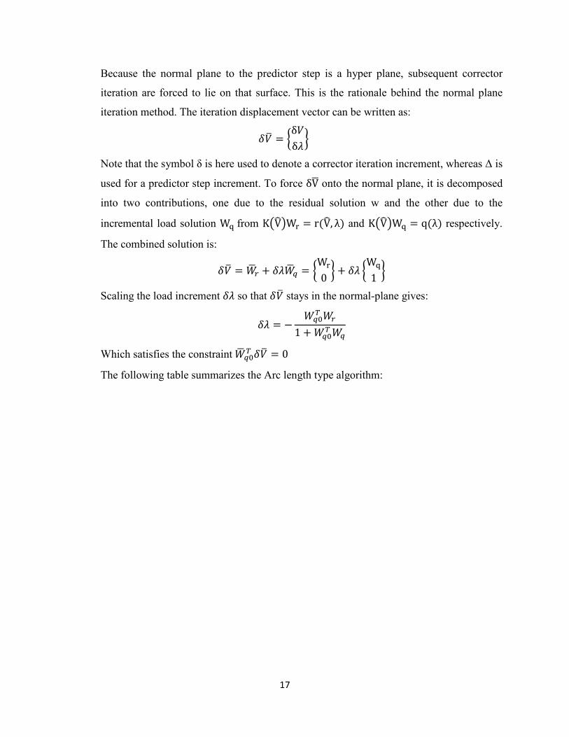
Because the normal plane to the predictor step is a hyper plane, subsequent corrector
iteration are forced to lie on that surface. This is the rationale behind the normal plane
iteration method. The iteration displacement vector can be written as:
b+_ � `c+c'a� Note that the symbol δ is here used to denote a corrector iteration increment, whereas ∆ is
used for a predictor step increment. To force cjh onto the normal plane, it is decomposed
into two contributions, one due to the residual solution w and the other due to the
incremental load solution kl�from mejnfko � L�jn� p� and mejnfkl � q�p� respectively.
The combined solution is:
b+_ � gh < b'gh% � `ko� a < b' `kl$ a Scaling the load increment b' so that b+_ stays in the normal-plane gives:
b' � � g%E- g $ <g%E-g%
Which satisfies the constraint�gh%E- b+_ � �
The following table summarizes the Arc length type algorithm:

18
Predictor step with arc length rD:
Set +� � mejnf��q�p� For n= 1 to number of increments
Solve mejnfklE � q�p��with respect to klE
Set � � s$ <g%E-g%E
If g%E- +E t $��^' � uv"
Else ^' � � uv"
Set +� � �^'klE
Update ' w ' < ^'�and +d w +d < �^'kl
Corrector iterations:
For i=1 to max iteration number for correction
Set kl � mejnf��q�p� Set ko � �mejnf��L�jn� '� Set b' � � xyz{ x|�Yxyz{ xy
Set ' � ' < b'
Set jn � jn < �goY�b'gl� Until }��jn� '�} ~ � � is the force residual convergence criterion
End
End
Arc length type algorithm

19
3- The formulation of the 4-node Quad. Iso-p. Element:
3-1-Geometric relations:
In 4-node quadrilateral Iso Parametric element, the nodal coordinates of any arbitrary point in the
element is interpolated from the coordinates of corner nodes by some bilinear shape functions.
The nodal coordinates can be either in the reference configuration or current configuration.
: � � :�!��� C � � C�!��� $ � � �!��� � � � ��!��� ] � � ��!��� $ � � �!���
(:� C��and (� � ]�are the nodal coordinates in reference and current configurations respectively.
The quad element is shown in the following figure:
Iso-P quad element
3-2-Displacement interpolation:
The displacement of any arbitrary point in the element can also be interpolated from the
displacements of the corner nodes by the same shape functions that are used in geometric
relations. �� � � ���!��� �� � � ���!���
ux=x-X uy=y-Y

20
3-3-Shape functions:
The following bilinear shape functions are used for interpolation:
��! � �� �$ � ���$ � �� ��! � �� �$ < ���$ � �� ��! � �� �$ < ���$ < �� ��! � �� �$ � ���$ < ��
3-4-Partial derivative computations:
Partial derivatives of shape functions with respect to the Cartesian coordinates X and Y are
required for the strain and stress calculations. Because shape functions are not directly functions
of X and Y but of the natural coordinates ξ and η, the determination of Cartesian partial
derivatives is not trivial. The derivative calculation procedure is presented below for the case of
an arbitrary Iso-parametric quadrilateral element with n nodes.
3-5-Jacobian:
In quadrilateral element derivations we will need the Jacobian of two-dimensional
transformations that connect the differentials of {x, y} to those of {ξ, η} and vice-versa. Using
the chain rule:
� � ��;�A������� � ��;�� �A���;�� �A��� � 6��� ������ ���8 ,����� � ��������;�A� � ����; ���;���A ���A
� � ��!���� 6 ��� �������� ��� 8
3-6-Shape function derivative:
The shape functions of a quadrilateral element are expressed in terms of the quadrilateral
coordinates ξ and η. The derivatives with respect to X and Y are given by the chain rule:
�����; � ������ ���; < ������ ���;
�����A � ������ ���A < ������ ���A

21
3-7-Derivatives of Cartesian coordinates w.r.t. natural coordinates:
:� � ��:���
�!� ���������������:� � ��:���
�!� � C� � ��C�
���!� �������������������C� � ��C�
���!� �
3-8-Displacement derivative:
The displacement derivatives are used in the nonlinear formulations, so it is worth deriving the derivatives of displacements with respect to initial configuration as below:
�;!: � �������
�!� � �: <�������
�!� � �:�������������;!C � �������
�!� � �C <�������
�!� � �C
�A!: � ���A���
�!� � �: <���A���
�!� � �:��������������A!C � ���A���
�!� � �C <���A���
�!� � �C
3-9-Strain derivatives with respect to state variables:
9::�; � ��;:�; < ��;:�; �;: < ��A:�; �A:
9::�A � ��;:�A < ��;:�A �;: < ��A:�A �A:
9CC�A � ��AC�A < ��AC�A �AC < ��;C�A �;C
9CC�; � ��AC�; < ��AC�; �AC < ��;C�; �;C
9:C�; � ��� > ��;C�; < ��A:�;B < ��� > ��;:�; �;C < ��;C�; �;: < ��AC�; �A: < ��A:�; �AC B 9:C�A � ��� > ��;C�A < ��A:�AB < ��� > ��;:�A �;C < ��;C�A �;: < ��AC�A �A: < ��A:�A �AC B
All above derivatives are used to measure the GL strain tensor for each element which is used to
determine the internal strain energy as discussed before.

22
The gradient of the strain energy for each element gives the residual and tangent stiffness matrix.
The resulting r and k of each element is assembled into the r and K of the whole structure. The
process will be explained in details in the further sections.
3-10-Selective Reduced Integration: (SRI method)
In Quadrilateral element if the element is very thin, the element becomes stiff in inplane bending,
which is called the “shear locking” phenomenon. In order to get rid of the shear locking, the
selective reduced integration is used.
In this method the E matrix is split into a volumetric and a shear portion. Thus, the internal
energy is also split into a volumetric and a shear part. 1x1 node Gauss rule is applied on the
shear portion and 2x2 node Gauss rule is applied on the volumetric part when we integrate the
energy over the entire volume of the element.
The E tensor for the plane stress problem is split as below:
F� � F=�$ < G� H= � �� = �� � $I <FG$ � G� H$ $ �$ $ �� � �I � F� < F�

23
4-Explanation of the FEM code (assumptions and abilities of the code)
The code consists of three major parts which are:
• Preprocessing (Reading input data) :
1. Getting the material properties:
§ Elastic modulus of material
§ Poisson’s ratio
2. Prestress value in 3 directions: It is a vector with initial stress in reference
configuration in 3 Cartesian directions. Dimension is 3x1
3. Number of elements
4. Number of nodes
5. Number of unrestrained degrees of freedom
6. Nodal coordinates: The dimension of this matrix is (number of node x 2)
7. Applied loads on nodes: The dimension of this matrix is (the number of nodes that
have forces on x 3): The first component of each row is the node number and the
other two components of each row correspond to the loads in X and Y directions
respectively.
8. Connectivity between the nodes: that shows that every element is located between
which four nodes. The nodes assignment is counterclockwise. The dimension of
connectivity matrix is (number of element x 4).
9. ID matrix: that assigns an equation number to each degree of freedom of all the
nodes. For example if node one is restrained in X direction and free in Y
direction, the first column of the ID Matrix is��E��. The dimension of ID is ( 2 x
number of nodes)
10. Getting the data required for iteration procedure:
§ rD : the Arc length
§ VO�TSQL� the maximum number of iteration in corrector step
§ Conv_eps1: the convergence criterion for force and displacement residuals
§ Conv_eps1: the convergence criterion for energy
§ Inc_num: the number of increments

24
§ ' : initial value for ' at the beginning of the iterations
§ �: initial value of u vector at the beginning of the iterations. The length of
u is equal to the number of free degrees of freedom.
• Solution:
1. Setting up the load vector: that reduces the degrees of freedom which are
restrained. The length of this vector is equal to the number of free degrees of
freedom or the number of unknowns.
2. Setting up the LM matrix: In this matrix every column corresponds to one
element. The rows of each column give the equation numbers of the corner nodes
in X and Y directions (as set up in ID before). The nodes are assigned in
counterclockwise direction. The dimension of LM matrix is (8 x number of
elements)
3. Determining the reference residual vector and tangent stiffness matrix for the
whole structure considering u and '�equal to zero.
§ Calling “Global_r_k” function: this function computes the r and K for the
whole structure. The followings are the adopted procedures in this
function to compute the global r and K :
o Loop over the number of elements
§ Setting up the u vector for each element
§ Setting up the nodal Cartesian coordinates vector for each
element
§ Calling “r_and_k” function: this function calculates the r and k
for each element
o Applying “Selective Reduced Integration” to measure
the internal energy over the volume of the element.
§ Calling “one_node_Gauss” and “two_node
_Gauss” functions to do all the required
calculations in the element level to measure the
derivatives of displacement, strains, internal
energy and in the end the re a and ke.
§ Establishing the global r vector and global K tensor

25
§ Assembling the local r and k to the global ones.
o end the loop
§ Subtracting the ' � ) from the r_global to get to the assembled
global r vector for the whole system.
4. Starting the iterations as mentioned in the table for arc length type algorithm.
§ In this part the r and K will be updated due to changes in u vector and p
• Post-processing:
1-storing all the incremented ' and displacements in some vectors
2-plotting the equilibrium path for each degree of freedom (in ' and displacement space)
The following flow chart summarizes different parts of the code in a hierarchical fashion:

26

27

28
5-Verification of the code:
5-1-verification examples:
In order to verify the code, a slender column is modeled with 6 quadrilateral elements and the
buckling load of the system is determined. The column behaves as a clamped bar since it is
restrained at the end against rotation and displacement. The size of each element is .25x3 meter.
So the dimension of the column in XY plane is 9.0 by 0.5 which looks very slender. The
Poison’s ratio and the E modulus of the structure are 0.2 and 1.0 KN/m2 respectively in all the
calculations. The shape of the structure is shown below:
Geometry of the column
The buckling load of the above-shown column is determined by applying a horizontal load on
nodes 4,8,12 and a very small vertical load on node 12 to perturb the tip of the column.
The following table shows the nodal forces on nodes:
Node 4 8 12
load X direction P1=-0.25 P2=-0.5 P1=-0.25
Y direction 0 0 P0=0.00001
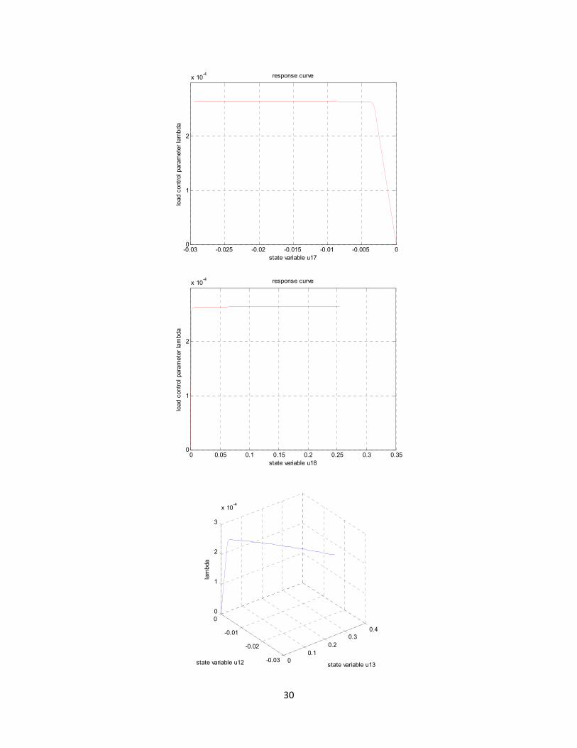
The resultant response curves for nodes 8 (DOF’s 12, 13) and 11(DOF’s 17, 18) in both X & Y
directions are plotted below:

29
-0.025 -0.02 -0.015 -0.01 -0.005 00
1
2
x 10-4
state variable u12
load control parameter lambda
response curve
0 0.1 0.2 0.3 0.4 0.5 0.6 0.70
1
2
x 10-4
state variable u13
load control parameter lambda
response curve
00.2
0.40.6
0.8
-0.03
-0.02
-0.01
00
1
2
3
x 10-4
state variable u13state variable u12
lambda
30
-0.03 -0.025 -0.02 -0.015 -0.01 -0.005 00
1
2
x 10-4
state variable u17
load control parameter lambda
response curve
0 0.05 0.1 0.15 0.2 0.25 0.3 0.350
1
2
x 10-4
state variable u18
load control parameter lambda
response curve
00.1
0.20.3
0.4
-0.03
-0.02
-0.01
00
1
2
3
x 10-4
state variable u13state variable u12
lambda

31
As can be seen the buckling load in which the response curve has an abrupt change in the
direction is =� � � $��� KN. Now we calculate the analytical buckling load for this clamped
column to compare the results:
�¡ � ��F¢&£� � ¤��¥ � $������
Where:
E=1 KN/m2 L=9.0 I=1/12x1x.53=0.0104 m4
The reasons of the difference between the analytical and numerical solutions can be the effect of
poison’s ratio and the finite element approximation. On the other hand, in analytical solution we
neglect the shear effect. Considering these facts, the results of FEM code are acceptable.
5-2-some specific load combinations on the column:
Moreover, Different nodal forces are applied on the structure and the corresponding response
curves are plotted in (' , u) space for nodes 4,8,12.
The following pictures are the response curves for different values of forces on nodes 4,8,12 in X
& Y directions.
Node 4 8 12
load X direction P1=-0.25 P2=-0.5 P1=-0.25
Y direction 0 0 P0=0.0
-25 -20 -15 -10 -5 0
-0.1
0
0.1
0.2
0.3
0.4
0.5
0.6
state variable u12
load control parameter lambda
response curve

32
-6 -5 -4 -3 -2 -1 0 1
x 10-12
-0.1
0
0.1
0.2
0.3
0.4
0.5
0.6
state variable u13
load control parameter lambda
response curve
-16 -14 -12 -10 -8 -6 -4 -2 0-0.1
0
0.1
0.2
0.3
0.4
0.5
0.6
state variable u17
load control parameter lambda
response curve
-0.04 -0.03 -0.02 -0.01 0 0.01 0.02 0.03-0.1
0
0.1
0.2
0.3
0.4
0.5
0.6
state variable u18
load control parameter lambda
response curve

33
Node 4 8 12
load X direction P1=0.25 P2=0.5 P1=0.25
Y direction 0 0 P0=0.0
0 5 10 15 20 250
2
4
6
8
10
12
state variable u12
load control parameter lambda
response curve
-0.5 0 0.5 1 1.5 2 2.5 3 3.5 4
x 10-15
0
2
4
6
8
10
12
state variable u13
load control parameter lambda
response curve

34
0 5 10 150
2
4
6
8
10
12
state variable u17
load control parameter lambda
response curve
-0.35 -0.3 -0.25 -0.2 -0.15 -0.1 -0.05 00
2
4
6
8
10
12
state variable u18
load control parameter lambda
response curve
35
Node 4 8 12
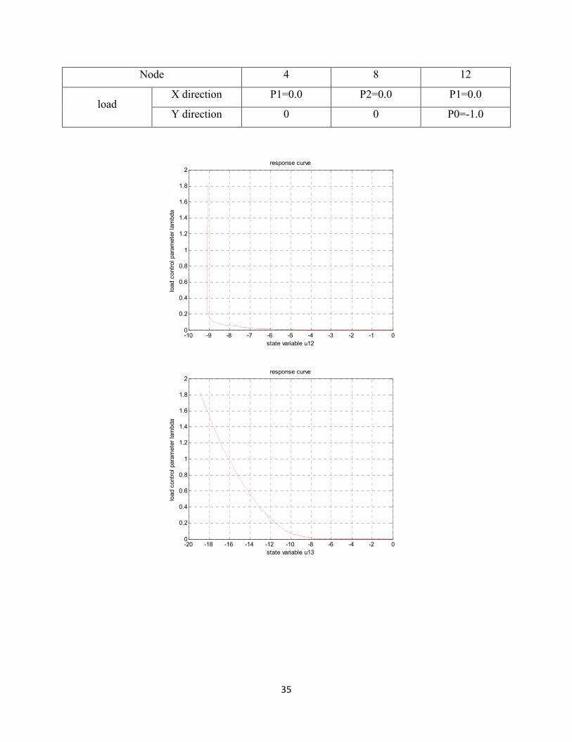
load X direction P1=0.0 P2=0.0 P1=0.0
Y direction 0 0 P0=-1.0
-10 -9 -8 -7 -6 -5 -4 -3 -2 -1 00
0.2
0.4
0.6
0.8
1
1.2
1.4
1.6
1.8
2
state variable u12
load control parameter lambda
response curve
-20 -18 -16 -14 -12 -10 -8 -6 -4 -2 00
0.2
0.4
0.6
0.8
1
1.2
1.4
1.6
1.8
2
state variable u13
load control parameter lambda
response curve

36
-6 -5 -4 -3 -2 -1 0 10
0.2
0.4
0.6
0.8
1
1.2
1.4
1.6
1.8
2
state variable u17
load control parameter lambda
response curve
-14 -12 -10 -8 -6 -4 -2 00
0.2
0.4
0.6
0.8
1
1.2
1.4
1.6
1.8
2
state variable u18
load control parameter lambda
response curve

37
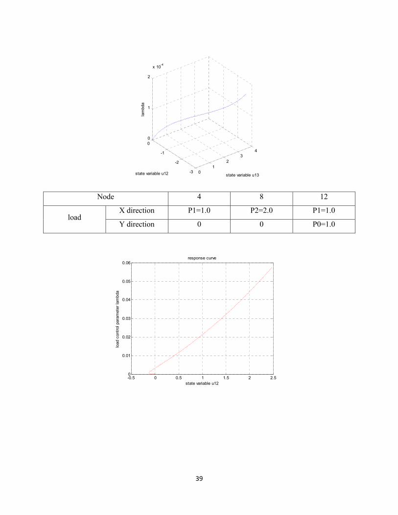
Node 4 8 12
load X direction P1=-1.0 P2=-2.0 P1=-1.0
Y direction 0 0 P0=1.0
-7 -6 -5 -4 -3 -2 -1 00
0.2
0.4
0.6
0.8
1
1.2
1.4
1.6
1.8x 10
-4
state variable u12
load control parameter lambda
response curve
0 1 2 3 4 5 6 7 80
0.2
0.4
0.6
0.8
1
1.2
1.4
1.6
1.8x 10
-4
state variable u13
load control parameter lambda
response curve

38
02
46
8
-8
-6
-4
-2
00
1
2
x 10-4
state variable u13state variable u12
lambda
-3 -2.5 -2 -1.5 -1 -0.5 00
0.2
0.4
0.6
0.8
1
1.2
1.4
1.6
1.8x 10
-4
state variable u17
load control parameter lambda
response curve
-3 -2.5 -2 -1.5 -1 -0.5 00
0.2
0.4
0.6
0.8
1
1.2
1.4
1.6
1.8x 10
-4
state variable u17
load control parameter lambda
response curve
39
Node 4 8 12
load X direction P1=1.0 P2=2.0 P1=1.0
Y direction 0 0 P0=1.0
01
23
4
-3
-2
-1
00
1
2
x 10-4
state variable u13state variable u12
lambda
-0.5 0 0.5 1 1.5 2 2.50
0.01
0.02
0.03
0.04
0.05
0.06
state variable u12
load control parameter lambda
response curve

40
0 0.5 1 1.5 2 2.5 30
0.01
0.02
0.03
0.04
0.05
0.06
state variable u13
load control parameter lambda
response curve
-0.2 0 0.2 0.4 0.6 0.8 1 1.2 1.4 1.6 1.80
0.01
0.02
0.03
0.04
0.05
0.06
state variable u17
load control parameter lambda
response curve
0 0.2 0.4 0.6 0.8 1 1.2 1.4 1.6 1.8 20
0.01
0.02
0.03
0.04
0.05
0.06
state variable u18
load control parameter lambda
response curve
41
As we can see in the responses, by changing the load combinations on different nodes we can
capture limit points, buckling point (bifurcations) and the turning points. The slender column is a
good exercise for capturing all the important points that may occur in nonlinear analysis.
The arc length type solution algorithm with hyperplane method for corrective stage gives
reasonable results for this problem.
5-2- Assumption of the code:
The following are the assumptions made in developing the nonlinear quadrilateral Iso-P element:
1. The material is elastic with finite deformation but small strains. Hence the hook
constitutive equation is still valid for this element. As we know this code is not good for
modeling the elastic membranes with large strains such as rubbers or polymers.
2. The loads are assumed to be conservative. The code is not capable of solving systems
with non-conservative loads such as wind or hydrostatic loads which change direction
along with the deformation of the structure.
3. The material is assumed to be compressible. This code is not suitable to model the
material with Poisson’s ratio close to 0.5.
4. The structure has 2D plane stress behavior. For plane strain problems we should add the
corresponding E tensor for plane strain behavior to the code.
5. Only one stage is defined in this code. The only force that can be applied is the nodal
forces.
5-3- Directions for further research:
The following issues could be investigated and added to improve the code:
§ Extending the element to 3D
§ Adding drilling degrees of freedom to each node. This has been done by
Haugen in 1994 but the kinematic description was Corotational which
assumed a linearized strain in the formulation. Since the resulting element
will no longer be compatible due to the drilling degrees of freedom, the
large strain and finite rotations must be investigated carefully.

42
§ Changing the constitutive relation in such a way that the element can
model the finite deformations with large strains such as rubbers and
polymers.
§ Adding plasticity to the code.( material nonlinearity)
6-Appendix A: The code Matlab file