Embed Size (px)
Citation preview

HAL Id: hal-02918610https://hal.archives-ouvertes.fr/hal-02918610
Submitted on 20 Aug 2020
HAL is a multi-disciplinary open accessarchive for the deposit and dissemination of sci-entific research documents, whether they are pub-lished or not. The documents may come fromteaching and research institutions in France orabroad, or from public or private research centers.
L’archive ouverte pluridisciplinaire HAL, estdestinée au dépôt et à la diffusion de documentsscientifiques de niveau recherche, publiés ou non,émanant des établissements d’enseignement et derecherche français ou étrangers, des laboratoirespublics ou privés.
Distributed under a Creative Commons Attribution| 4.0 International License
Geometric Nonlinear Analysis of Timoshenko BeamsS. Amir Mousavi Lajimi
To cite this version:S. Amir Mousavi Lajimi. Geometric Nonlinear Analysis of Timoshenko Beams. [Technical Report]University of Waterloo. 2009. �hal-02918610�

Geometric Nonlinear Analysis OfTimoshenko Beams
with a comprehensive study of linear and nonlinear computationalmechanics of solids and structures
S.Amir Mousavi LajimiPhD Candidate
Department of Systems Design Engineering
Computational Solid MechanicsSpring 2009
Instructor: Professor Katerina D. Papoulia
University Of Waterloo
September 2009

AbstractThe linear �nite element analysis of solids and structures are discussed in the �rst part of the report. The�nite element formulations for a three dimensional problem is derived and signi�cant issues are addressed.Three di�erent types of elements, the bilinear iso-parametric quadrilaterals, the quadratic triangles andthe linear tetrahedrons are used to solve a linear plate problem and the results are compared.The analysis of a common geometric nonlinearity encountered in structural mechanics is dealt with in thesecond part of the report. A brief introduction to nonlinear analysis is provided, while the geometric non-linearity is discussed in detail. Timoshenko beam analysis is considered as the one dimensional version ofReissner-Mindlin plate theory and the nonlinear strain-displacement relation are treated in an appropri-ate way to avoid unrealistic simpli�cations. The force vector and tangent sti�ness matrix are derived andthe formulation is extended to implement the trigonometric basis functions. A major issue in geometricnonlinear analysis, namely locking, is addressed and reduced order integrations are implemented to avoidthe consequences. The convergence of the model is checked with available analytical solutions. An Eulermethod in combination with Newton-Raphson method is used to fully analyze the geometric nonlinearity.
Copyright ©2009 S. A. M. Lajimi

Contents
1 Introduction 11.1 Motivation . . . . . . . . . . . . . . . . . . . . . . . . . . . . . . . . . . . . . . . . . . . . 11.2 The Finite Element Method . . . . . . . . . . . . . . . . . . . . . . . . . . . . . . . . . . . 11.3 Report Organization . . . . . . . . . . . . . . . . . . . . . . . . . . . . . . . . . . . . . . . 2
I The Linear Computational Mechanics 32 Development of the Finite Element Method 4
2.1 Introduction . . . . . . . . . . . . . . . . . . . . . . . . . . . . . . . . . . . . . . . . . . . . 42.2 Basic Equations . . . . . . . . . . . . . . . . . . . . . . . . . . . . . . . . . . . . . . . . . . 4
2.2.1 Equilibrium Equations . . . . . . . . . . . . . . . . . . . . . . . . . . . . . . . . . . 42.2.2 Constitutive Relations . . . . . . . . . . . . . . . . . . . . . . . . . . . . . . . . . . 52.2.3 Strain-Displacement Relations . . . . . . . . . . . . . . . . . . . . . . . . . . . . . 62.2.4 Boundary Conditions . . . . . . . . . . . . . . . . . . . . . . . . . . . . . . . . . . 62.2.5 Compatibility Equations . . . . . . . . . . . . . . . . . . . . . . . . . . . . . . . . . 7
2.3 Formulations . . . . . . . . . . . . . . . . . . . . . . . . . . . . . . . . . . . . . . . . . . . 72.3.1 Di�erential Equation Methods . . . . . . . . . . . . . . . . . . . . . . . . . . . . . 72.3.2 Variational Methods . . . . . . . . . . . . . . . . . . . . . . . . . . . . . . . . . . . 72.3.3 Formulations of Finite Element Equations . . . . . . . . . . . . . . . . . . . . . . . 9
3 Elements and Interpolation Functions 123.1 Introduction . . . . . . . . . . . . . . . . . . . . . . . . . . . . . . . . . . . . . . . . . . . . 123.2 The Bilinear Quadrilateral Lagrangian Element . . . . . . . . . . . . . . . . . . . . . . . . 12
3.2.1 Element Shape Functions . . . . . . . . . . . . . . . . . . . . . . . . . . . . . . . . 123.2.2 Implementation . . . . . . . . . . . . . . . . . . . . . . . . . . . . . . . . . . . . . . 13
3.3 The Quadratic Triangular Element . . . . . . . . . . . . . . . . . . . . . . . . . . . . . . . 143.3.1 Geometry . . . . . . . . . . . . . . . . . . . . . . . . . . . . . . . . . . . . . . . . . 143.3.2 Element Shape Functions . . . . . . . . . . . . . . . . . . . . . . . . . . . . . . . . 143.3.3 Implementation . . . . . . . . . . . . . . . . . . . . . . . . . . . . . . . . . . . . . . 153.3.4 Gauss Quadrature for Triangular Elements . . . . . . . . . . . . . . . . . . . . . . 16
3.4 The Linear Tetrahedral (Solid) Element . . . . . . . . . . . . . . . . . . . . . . . . . . . . 173.4.1 Geometry . . . . . . . . . . . . . . . . . . . . . . . . . . . . . . . . . . . . . . . . . 173.4.2 Element Shape Functions . . . . . . . . . . . . . . . . . . . . . . . . . . . . . . . . 183.4.3 Implementation . . . . . . . . . . . . . . . . . . . . . . . . . . . . . . . . . . . . . . 18
4 Results 204.1 The Bilinear Quadrilateral Element . . . . . . . . . . . . . . . . . . . . . . . . . . . . . . . 204.2 The Quadratic Triangular Element . . . . . . . . . . . . . . . . . . . . . . . . . . . . . . . 214.3 The Linear Tetrahedral Element . . . . . . . . . . . . . . . . . . . . . . . . . . . . . . . . 224.4 Discussion . . . . . . . . . . . . . . . . . . . . . . . . . . . . . . . . . . . . . . . . . . . . . 23
i

II The Nonlinear Computational Mechanics 245 Nonlinear Finite Element Method 25
5.1 Introduction . . . . . . . . . . . . . . . . . . . . . . . . . . . . . . . . . . . . . . . . . . . . 255.2 Nonlinearities in Solid and Structural Mechanics . . . . . . . . . . . . . . . . . . . . . . . 255.3 Solution Procedures . . . . . . . . . . . . . . . . . . . . . . . . . . . . . . . . . . . . . . . 25
5.3.1 Geometric Nonlinearity . . . . . . . . . . . . . . . . . . . . . . . . . . . . . . . . . 265.3.2 Material Nonlinearity . . . . . . . . . . . . . . . . . . . . . . . . . . . . . . . . . . 26
6 Finite Element Analysis of Nonlinear Timoshenko Beams 276.1 Introduction . . . . . . . . . . . . . . . . . . . . . . . . . . . . . . . . . . . . . . . . . . . . 276.2 Background and Basic Equations . . . . . . . . . . . . . . . . . . . . . . . . . . . . . . . . 27
6.2.1 Straight Beams . . . . . . . . . . . . . . . . . . . . . . . . . . . . . . . . . . . . . . 276.2.2 Curved Beams . . . . . . . . . . . . . . . . . . . . . . . . . . . . . . . . . . . . . . 29
6.3 Beam Element and Interpolation Functions . . . . . . . . . . . . . . . . . . . . . . . . . . 316.4 Constitutive Relations . . . . . . . . . . . . . . . . . . . . . . . . . . . . . . . . . . . . . . 336.5 Finite Element Formulation of Equilibrium Equations . . . . . . . . . . . . . . . . . . . . 33
6.5.1 Tangent Sti�ness Matrix . . . . . . . . . . . . . . . . . . . . . . . . . . . . . . . . . 346.6 Reduced Numerical Integration . . . . . . . . . . . . . . . . . . . . . . . . . . . . . . . . . 37
7 Results 397.1 Cantilever with vertical tip load . . . . . . . . . . . . . . . . . . . . . . . . . . . . . . . . . 397.2 Quarter Circle Beam with Radial Tip Load . . . . . . . . . . . . . . . . . . . . . . . . . . 417.3 Discussion . . . . . . . . . . . . . . . . . . . . . . . . . . . . . . . . . . . . . . . . . . . . . 45
8 Conclusions 468.1 Conclusions . . . . . . . . . . . . . . . . . . . . . . . . . . . . . . . . . . . . . . . . . . . . 468.2 Future Works . . . . . . . . . . . . . . . . . . . . . . . . . . . . . . . . . . . . . . . . . . . 46
A Source codes 47A.1 Quadrilateral Bilinear Element . . . . . . . . . . . . . . . . . . . . . . . . . . . . . . . . . 47A.2 Quadratic Triangular Element . . . . . . . . . . . . . . . . . . . . . . . . . . . . . . . . . . 49A.3 Linear Tetrahedral Element . . . . . . . . . . . . . . . . . . . . . . . . . . . . . . . . . . . 50A.4 Nonlinear Timoshenko Beam Analysis . . . . . . . . . . . . . . . . . . . . . . . . . . . . . 51
B Locking 58
ii

List of Figures
3.1 Quadrilateral Lagrangian Element . . . . . . . . . . . . . . . . . . . . . . . . . . . . . . . 123.2 Quadratic Triangular Element . . . . . . . . . . . . . . . . . . . . . . . . . . . . . . . . . . 143.3 Triangular Coordinate . . . . . . . . . . . . . . . . . . . . . . . . . . . . . . . . . . . . . . 143.4 Linear Tetrahedron Element . . . . . . . . . . . . . . . . . . . . . . . . . . . . . . . . . . . 17
4.1 Thin plate under uniformly distributed load. . . . . . . . . . . . . . . . . . . . . . . . . . 204.2 Thin plate mesh using quadrilateral elements. . . . . . . . . . . . . . . . . . . . . . . . . . 214.3 Thin plate mesh using quadratic triangular elements. . . . . . . . . . . . . . . . . . . . . . 214.4 Thin plate mesh using linear tetrahedral elements . . . . . . . . . . . . . . . . . . . . . . . 22
6.1 The straight beam element . . . . . . . . . . . . . . . . . . . . . . . . . . . . . . . . . . . 286.2 The curved beam element . . . . . . . . . . . . . . . . . . . . . . . . . . . . . . . . . . . . 306.3 An automated code to produce Lagrangian basis functions. . . . . . . . . . . . . . . . . . 32
7.1 The cantilever straight beam. . . . . . . . . . . . . . . . . . . . . . . . . . . . . . . . . . . 397.2 The cantilever straight beam results, L/ℎ = 4 . . . . . . . . . . . . . . . . . . . . . . . . . 407.3 The cantilever straight beam results, L/ℎ = 10 . . . . . . . . . . . . . . . . . . . . . . . . 417.4 The cantilever straight beam results, L/ℎ = 50 . . . . . . . . . . . . . . . . . . . . . . . . 427.5 The quarter circle curved cantilever beam. . . . . . . . . . . . . . . . . . . . . . . . . . . . 437.6 The cantilever curved beam results . . . . . . . . . . . . . . . . . . . . . . . . . . . . . . . 437.7 The p-convergence of the results . . . . . . . . . . . . . . . . . . . . . . . . . . . . . . . . 447.8 The nonlinear force-displacement curve . . . . . . . . . . . . . . . . . . . . . . . . . . . . . 447.9 The di�erence between nonlinear and linear solution . . . . . . . . . . . . . . . . . . . . . 457.10 The force-displacement curve using Newton-Raphson method . . . . . . . . . . . . . . . . 45
iii

List of Tables
4.1 Global force and displacement vectors using Quadrilateral element . . . . . . . . . . . . . 214.2 Global force and displacement vectors for Triangular element . . . . . . . . . . . . . . . . 224.3 Global force and displacement vectors for Tetrahedral Element . . . . . . . . . . . . . . . 234.4 Convergence of the result for quadrilateral element . . . . . . . . . . . . . . . . . . . . . . 23
7.1 The material and geometric data of straight beams. . . . . . . . . . . . . . . . . . . . . . 40
iv

Chapter 1
Introduction
1.1 Motivation
The computational mechanics is associated with the implementations of the computational methodsin solving the problems of the mechanics including solid, structural, and �uid mechanics. Working incomputational mechanics is concerned with developing discrete models, numerical methods, and solutionprocedures for a wide range of problems arising from studying continuum mechanics.The mathematical descriptions or di�erential governing equations, are customarily referred to as thestrong form of a problem. The conclusive objective can be summarized as to have an algebraic equationor system of equations rather than di�erential governing equations which is ideal for implementationon the digital computer. These equations may be linear or nonlinear depending on the nature of theproblem 1.The most conventionally used solution technique is the �nite di�erence method, which makes use of thecalculus of �nite di�erences. The method is simply formulated and put into use by replacing di�erentialoperators with di�erence operators. However, the solutions are approximated for certain numbers ofnodes. Therefore, other methods such as the method of weighted residuals and the �nite element methodare implemented to approximate the solutions of a physical problem where a continuous solution is mostlydesired.While implementing some methods such as the method of weighted residuals is quite straightforwardfor simple domains, for complex domains such as curved boundaries it might not be convenient andadaptable. The �nite element method is introduced to overcome those impediments, and provides anaccessible method for many engineering problems. On the other hand, in the analysis of real structuresdealing with the existing nonlinearities is not avoidable. Thus, it is necessary to include di�erent typesof nonlinearities to simulate the true behavior of the structure. The nonlinear �nite element analysisprovides a powerful tool to deal with di�erent types of nonlinear problems.
1.2 The Finite Element Method
The domain is discretized to some smaller domains, where the error concerned with the discretizationof the domain can be reduced by reducing the size of the elements, the shape of the elements, and thenumber of the elements. The global system of equations is realized through a process called assembly,and the geometric boundary conditions are applied at the end before solving the system of algebraic
1The governing di�erential equations display what is expected regarding linearity or nonlinearity of the �nal form.
1

equations. Indeed, the procedure is unambiguous, except a nonlinearity appears ahead in the governingequations of the system.The genuine systems are always nonlinear, however linear solutions are easier to compute at lower costs.The linear solutions do satisfy the actual requirements to certain degrees, however to gain a better un-derstanding of the behavior of the continuum and physical phenomena a nonlinear analysis is imperative.A nonlinear di�erential equation results in a nonlinear algebraic system, where the solution should besought using some iterative procedures. Therefore, the computational cost will increase and some newissues such as stability and optimality of the result might arise.The main classes of nonlinearities are geometric nonlinearities and material nonlinearities. While, thelatter occur when the stress-strain or force-displacement law is not linear, or when material propertieschange with the applied loads, the former involves nonlinearities in kinematic quantities such as thestrain-displacement relations in solids. Such nonlinearities can occur due to large displacements, largestrains, large rotations, and so on. Contact can also be classi�ed as a geometric nonlinearity becausethe area of contact is a function of the deformation 1. The main objective of this work is to provide thenonlinear �nite element equations encountered when analyzing a Timoshenko beam. The nonlinearityappears when considering a nonlinear strain-displacement relation. Hence, the geometric nonlinearity isconsidered here.
1.3 Report Organization
The report is presented in two parts: the linear �nite element analysis and the nonlinear �nite elementanalysis. Development of the �nite element method for a linear analysis is described in chapter 2. Chapter3 includes a review of several types of elements and interpolation functions. In the �nal chapter of the �rstpart, chapter 4, the results of the linear �nite element analysis of a problem is presented. Second part,starts with an introduction to the nonlinear �nite element method in chapter 5. Chapter 6 is devoted tothe derivation of the nonlinear �nite element equations for Timoshenko beam. It includes the requiredformulations for analyzing the straight as well as curved beams, an explanation about the beam element,several types of shape functions and integration schemes. In chapter 7 the results are provided for twocases where a comparison is made between the linear and nonlinear solutions. Finally, the conclusionsand future works are brie�y mentioned in chapter 8.
1Contact can be considered in another class called nonlinear boundary conditions.
2

Part I
The Linear Computational Mechanics
3

Chapter 2
Development of the Finite ElementMethod
2.1 Introduction
One appreciates miscellaneous types of problems solved by the �nite element method in the �eld ofapplied mechanics including the linear analysis of solids and structures under small deformation, and thenonlinear analysis of solids and structures. In this chapter, we are dealing with the �nite element elasticanalysis of one-, two-, and three-dimensional problems.
2.2 Basic Equations
In solid and structural mechanics, the problem is primarily to �nd the displacement distributions andstresses under the external loads and boundary conditions. Therefore, the initial step would be to satisfythe equilibrium equations, that is considering an element of the material inside the body, it must be inequilibrium due to the internal forces (stresses) developed as a result of the external provocations.
2.2.1 Equilibrium Equations
When a body is in equilibrium, the force and moment equilibrium equations for the overall body have tobe satis�ed. This leads to the following equations for each point of a body,
∂¾xx
∂x+
∂¾xy
∂y+
∂¾zx
∂z+ bx = 0
∂¾xy
∂x+
∂¾yy
∂y+
∂¾yz
∂z+ by = 0 (2.1)
∂¾zx
∂x+
∂¾yz
∂y+
∂¾zz
∂z+ bz = 0
where ¾xx, ¾yy and ¾zz are the normal stresses, ¾xy, ¾yz and ¾zx are the shear stresses, and bx, by and bzare the body forces per unit volume acting along the x, y and z respectively.
4

2.2.2 Constitutive Relations
The secondary dependent variables are correlated to the primary dependent variables through appropriaterelations involving derivatives of the primary dependent variables. In addition, the constitution of thematerial must be taken into account. This is accomplished through the constitutive relations. Theconstitutive relations describe the response of a certain system or body to an applied loading. In the caseof linearly elastic materials, in a three-dimensional analysis, the stress-strain relations, or constitutiverelations, are given by Hook's law as
² =
⎧⎨⎩
²xx²yy²zz²xy²yz²zx
⎫⎬⎭
= [C]¾ ≡ [C]
⎧⎨⎩
¾xx
¾yy
¾zz
¾xy
¾yz
¾zx
⎫⎬⎭
(2.2)
where [C] is a matrix of elastic constants given by,
[C] =1
E
⎡⎢⎢⎢⎢⎢⎢⎣
1 −º −º 0 0 0−º 1 −º 0 0 0−º −º 1 0 0 00 0 0 2(1 + º) 0 00 0 0 0 2(1 + º) 00 0 0 0 0 2(1 + º)
⎤⎥⎥⎥⎥⎥⎥⎦
(2.3)
E is Young's modulus and º is Poisson's ratio of the material. Stresses are expressed in terms of strainsas,
¾ =
⎧⎨⎩
¾xx
¾yy
¾zz
¾xy
¾yz
¾zx
⎫⎬⎭
= [D]² ≡ [D]
⎧⎨⎩
²xx²yy²zz²xy²yz²zx
⎫⎬⎭
(2.4)
[D] =E
(1 + º)(1− 2º)
⎡⎢⎢⎢⎢⎢⎢⎢⎣
1− º º º 0 0 0º 1− º º 0 0 0º º 1− º 0 0 0
0 0 0 (1−º)2 0 0
0 0 0 0 (1−º)2 0
0 0 0 0 0 (1−º)2
⎤⎥⎥⎥⎥⎥⎥⎥⎦
(2.5)
Two states of stress distribution are possible in two-dimensional problems, namely, plane stress and plainstrain. The plane strain assumption is valid when the body is very long in one direction and its geometryand loading do not vary considerably in the longitudinal direction. For example, the analysis of dams andcylinder can be made using the plane strain assumption. The dependent variables are considered to befunctions of two independent directions, say x and y, provided a section far from the ends is considered.In this case the stress-strain relation is given by
¾ = [D]² (2.6)with,
[D] =E
(1 + º)(1− 2º)
⎡⎢⎣1− º º 0º 1− º 0
0 0 (1−º)2
⎤⎥⎦ (2.7)
5

The z-component of the stress will be nonzero and is given by
¾zz = º(¾xx + ¾yy
)(2.8)
and ¾yz = ¾zx = 0.The premise of the plane stress is valid for bodies with one small dimension in one of the coordinatedirections. For instance, in the analysis of thin plates when loaded in the plane the plane stress assumptionis justi�ed to be used. In plane stress distribution, it is assumed that
¾zz = ¾yz = ¾zx = 0 (2.9)
where z represents the perpendicular direction to the plane of the plate. In this case, the stress-strainrelation is given by
¾ = [D]² (2.10)
with,
[D] =E
1− º2
⎡⎢⎣1 º 0º 1 00 0 1−º
2
⎤⎥⎦ (2.11)
In the case of plane stress, the component of strain in the z- direction will be nonzero and is given by
²zz = − º
E
(¾xx + ¾yy
)(2.12)
and ²yz = ²zx = 0.
2.2.3 Strain-Displacement Relations
Strains are induced in a body during the change of its shape as a result of an imposed set of loads. Thesestrains vary through the volume of the body and can be related to the displacements at each point of thebody. De�ning u, v,and w as three components of displacements parallel to the x, yand z directions, thenormal strains in x, yand z directions are computed by
²xx =∂u
∂x, ²yy =
∂v
∂y, ²zz =
∂w
∂z(2.13)
The shear strain is de�ned as the decrease in the right angle between two �bers which were at right anglesto each other before deformation. Therefore, shear strains in the xy, yz and zx planes are
²xy =∂u
∂y+
∂v
∂x, ²yz =
∂v
∂z+
∂w
∂y, ²zx =
∂w
∂x+
∂u
∂z(2.14)
2.2.4 Boundary Conditions
Boundary conditions are divided to two major categories: the forced, geometric or Dirichlet boundaryconditions which are de�ned as displacement boundary conditions, and natural, physical, or Neumannboundary conditions which are restrictions on the surface traction or stresses. The boundary conditions ondisplacements require the body or structure to take on prede�ned displacements or de�ections at certainpoints, while the natural boundary conditions require that the stresses induced must be in equilibriumwith the external forces applied at certain points on the boundary of the body.
6

2.2.5 Compatibility Equations
The displacement �eld inside a body or structure must be continuous as well as single valued. This isknown as the condition of the compatibility. The condition of compatibility can be described from adi�erent point of view. It can be observed from Eqs. (2.13) and (2.14) that the three strains ²xx, ²yyand ²xy are derived from only two displacements u and v. This implies that there should be a relationbetween ²xx, ²yy and ²xy if these strains correspond to a compatible deformation. This relation is calledthe �compatibility equation� . In three-dimensional elasticity problems, there are totally six compatibilityequations to be satis�ed. In the case of two-dimensional plane strain problems, a single equation mustbe met as
∂2²xx∂y2
+∂2²yy∂x2
=∂2²xy∂x∂y
(2.15)
For plane stress problems, the equations are expressed as
∂2²xx∂y2
+∂2²yy∂x2
=∂2²xy∂x∂y
,∂2²zz∂y2
=∂2²zz∂x2
=∂2²zz∂x∂y
(2.16)
In the case of one-dimensional problems the condition of compatibility is automatically satis�ed.
2.3 Formulations
Most of the solid and structural mechanics problems can be formulated starting from either the governingdi�erential equation of the problem using, for example, the principle of virtual work, or a variationalprinciple such as the principle of minimum potential energy. In the following a brief description of bothapproaches are provided.
2.3.1 Di�erential Equation Methods
In this type of formulations, a method such as Galerkin method is used for �nding an approximate solutionto a di�erential equation. Therefore, the approach is concerned with the direct use of the di�erentialequation; it does not require the existence of a functional. The Galerkin method is probably the mostpopular one in this category. Application of the Galerkin method requires that the following conditionsbe satis�ed [3] (as cited in [7]):
� The weighting or test functions are chosen from the same set as the trial functions.� The trial and test functions must be linearly independent.� The trial and test functions should be chosen from the �rst P functions of a complete set of functions.� The trial functions should exactly satisfy the boundary conditions and, if applicable, the initial
conditions.
2.3.2 Variational Methods
Using variational methods requires having a correct functional which gives the corresponding �nite el-ement equations when �nding the stationary point of it. There are several functionals to be used inmechanics such as the principle of minimum potential energy or Hamilton's principle which are suc-cinctly explained here.
7

Principle of Minimum Potential Energy
The potential energy of an elastic body, Π, is expressed as
Π = U −W (2.17)
where U is the strain energy and W is the work done on the body by the external forces. The principle ofminimum potential energy states that of all displacements satisfying the given compatibility, kinematicor boundary conditions those which satisfy the equilibrium equations make the potential energy assumea minimum value. Therefore, at equilibrium
±Π = ±U − ±W = 0 (2.18)
where ± shows the �rst variation taken with respect to the displacements. The strain energy of a linearelastic body is de�ned as
U =1
2
∫∫∫
V
²T¾ dV (2.19)
where V is the volume of the body. Using the stress-strain relation, Eq.(2.4), the strain energy can beexpressed as
U =1
2
∫∫∫
V
²T [D]²dV (2.20)
The work done by the external forces is computed using
W =
∫∫∫
V
bT ddV +
∫∫
St
tT ddSt (2.21)
where
b =
⎧⎨⎩bxbybz
⎫⎬⎭ (2.22)
is known as the body force vector,
t =
⎧⎨⎩txtytz
⎫⎬⎭ (2.23)
is the vector of prescribed surface traction de�ned on St, and
d =
⎧⎨⎩uvw
⎫⎬⎭ (2.24)
is the vector of displacements. When the principle of minimum potential energy is used to derive the �niteelement equations, we assume a simple form of variation for the displacement �eld within each elementand derive conditions which will minimize the corresponding functional, Π.The resulting equations arethe approximate equilibrium equations while the compatibility conditions are identically satis�ed.
8

Hamilton's Principle
Hamilton's principle states that of all admissible con�gurations that a body can take as it moves fromcon�guration a at time t1 to con�guration b at time t2, the path that satis�es the Newton's law at eachinstant during the interval (and is thus the actual locus of con�gurations) is the path that extremizes thetime integral of the Lagrangian during the interval. Therefore, Hamilton's principle can be stated as
±
t2∫
t1
L dt = 0 (2.25)
where the Lagrangian (L) is de�ned as
L = T − U (2.26)
The kinetic energy (T ) of a body is given by
T =1
2
∫∫∫
V
½dTddV (2.27)
where ½ is the density of the material and d = {u, v, w}T is the vector of velocity components at anypoint inside the body. The potential energy can be found from Eqs. (2.17) - (2.21). This variationalprinciple is used for dynamics problems.
Other Variational Principles
There are several other variational principles such as the principle of minimum complementary energy andthe minimum of Reissner energy. To derive the �nite element equations using the principle of stationaryReissner energy, a form of the variation for both displacement and stress �elds within the element isassumed. This leads to the mixed method of �nite element analysis.
2.3.3 Formulations of Finite Element Equations
The principle of minimum potential energy is used for deriving the equilibrium equations for a three-dimensional problem. The nodal degrees of freedom are treated as unknowns in this formulation. The�nal form of equilibrium equations can be obtained by setting the �rst partial derivatives of Π withrespect to each nodal degrees of freedom equal to zero. The various steps associated the derivation of theequilibrium equations are summarized below.
� The body or structure is divided into ne �nite elements.� The displacement model within an element e is assumed as
d =
⎧⎨⎩u(x, y, z)v(x, y, z)w(x, y, z)
⎫⎬⎭ = [N ]de (2.28)
where de is the vector of nodal displacement degrees of freedom of the element and [N ] is the matrixof shape functions.
� The element sti�ness matrix and force vectors are to be derived. The potential energy of an elemente is expressed as
Πe =1
2
∫∫∫
V e
²T [D]²dV −∫∫
Set
dT t dSt −∫∫∫
V e
dT bdV (2.29)
9
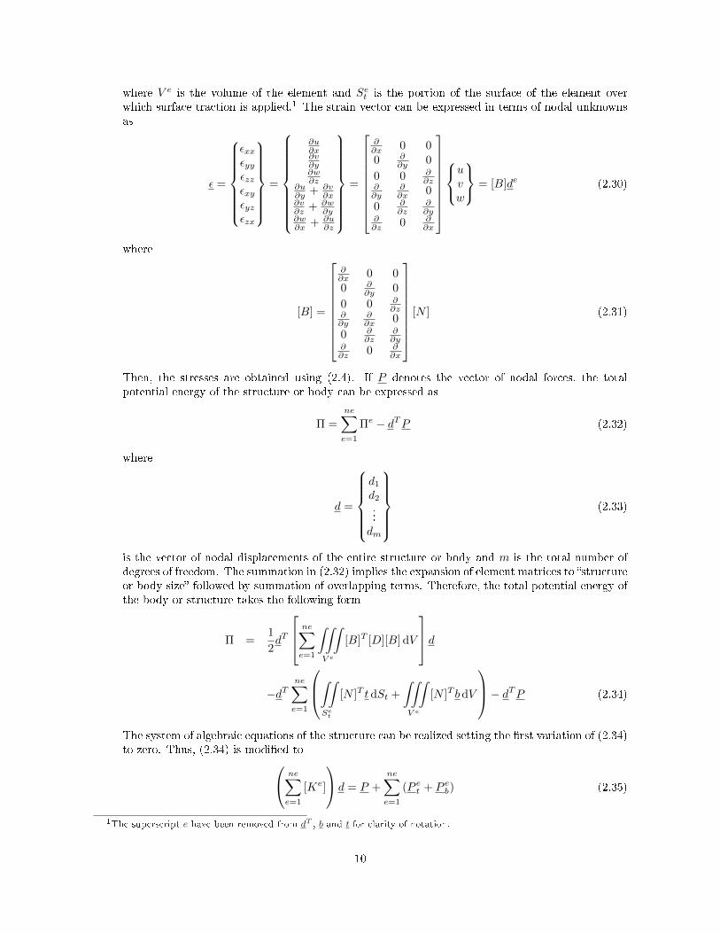
where V e is the volume of the element and Set is the portion of the surface of the element over
which surface traction is applied.1 The strain vector can be expressed in terms of nodal unknownsas
² =
⎧⎨⎩
²xx²yy²zz²xy²yz²zx
⎫⎬⎭
=
⎧⎨⎩
∂u∂x∂v∂y∂w∂z
∂u∂y + ∂v
∂x∂v∂z + ∂w
∂y∂w∂x + ∂u
∂z
⎫⎬⎭
=
⎡⎢⎢⎢⎢⎢⎢⎢⎢⎣
∂∂x 0 00 ∂
∂y 0
0 0 ∂∂z
∂∂y
∂∂x 0
0 ∂∂z
∂∂y
∂∂z 0 ∂
∂x
⎤⎥⎥⎥⎥⎥⎥⎥⎥⎦
⎧⎨⎩uvw
⎫⎬⎭ = [B]de (2.30)
where
[B] =
⎡⎢⎢⎢⎢⎢⎢⎢⎢⎣
∂∂x 0 00 ∂
∂y 0
0 0 ∂∂z
∂∂y
∂∂x 0
0 ∂∂z
∂∂y
∂∂z 0 ∂
∂x
⎤⎥⎥⎥⎥⎥⎥⎥⎥⎦
[N ] (2.31)
Then, the stresses are obtained using (2.4). If P denotes the vector of nodal forces, the totalpotential energy of the structure or body can be expressed as
Π =
ne∑e=1
Πe − dTP (2.32)
where
d =
⎧⎨⎩
d1d2...
dm
⎫⎬⎭
(2.33)
is the vector of nodal displacements of the entire structure or body and m is the total number ofdegrees of freedom. The summation in (2.32) implies the expansion of element matrices to �structureor body size� followed by summation of overlapping terms. Therefore, the total potential energy ofthe body or structure takes the following form
Π =1
2dT
⎡⎢⎣
ne∑e=1
∫∫∫
V e
[B]T [D][B] dV
⎤⎥⎦ d
−dTne∑e=1
⎛⎜⎝∫∫
Set
[N ]T t dSt +
∫∫∫
V e
[N ]T b dV
⎞⎟⎠− dTP (2.34)
The system of algebraic equations of the structure can be realized setting the �rst variation of (2.34)to zero. Thus, (2.34) is modi�ed to
⎛⎝
ne∑e=1
[Ke]
⎞⎠ d = P +
ne∑e=1
(P et + P e
b) (2.35)
1The superscript e have been removed from dT , b and t for clarity of notation.
10

where
[Ke] =
∫∫∫
V e
[B]T [D][B] dV (2.36)
is the element sti�ness matrix,
P et =
∫∫
Set
[N ]T t dSt (2.37)
is the element load vector due to the surface traction and
P eb =
∫∫∫
V e
[N ]T bdV (2.38)
represents the element load vector due to the body forces.� The global system of equations can now be expressed as
[K] d = F (2.39)
where
[K] =
ne∑e=1
[Ke] assembled sti�ness matrix (2.40)
and
F = P +
ne∑e=1
P eb +
ne∑e=1
P et assembled nodal load vector (2.41)
� The solution for the nodal displacements can be obtained after solving (2.39). However, this shouldbe done after applying the boundary conditions.
� The outputs from last step may further be post-processed to obtain stresses, strains, element de-formations and etc.
11

Chapter 3
Elements and Interpolation Functions
3.1 Introduction
This chapter continues with the computer implementation of the two- and three-dimensional �nite el-ements. It covers the derivation of the �nite element equations for bilinear quadrilateral Lagrangianelement, quadratic triangular element and linear tetrahedral (solid) element. The area and tetrahedralcoordinates are introduced, numerical integration for the triangular geometry is de�ned, and sti�nessmatrices are computed.
3.2 The Bilinear Quadrilateral Lagrangian Element
3.2.1 Element Shape Functions
The schematic of a quadrilateral element is shown in Fig. 3.1. The bilinear Lagrangian element isconsidered as a combination of two linear elements in two perpendicular directions, r and s, in elementcoordinate system.
1 2
34
r
s
Figure 3.1: Quadrilateral Lagrangian Element
Considering a linear approximation of trial function, the element shape function are expressed as
N1(r, s) =
[1
2(1− r)
] [1
2(1− s)
](3.1)
N2(r, s) =
[1
2(1 + r)
] [1
2(1− s)
](3.2)
12

N3(r, s) =
[1
2(1 + r)
] [1
2(1 + s)
](3.3)
N4(r, s) =
[1
2(1− r)
] [1
2(1 + s)
](3.4)
where r and s denote the natural coordinates of the element. For an iso-parametric element, eachCartesian coordinate is interpolated using
x = N1(r, s)x1 +N2(r, s)x2 +N3(r, s)x3 +N4(r, s)x4 (3.5)y = N1(r, s)y1 +N2(r, s)y2 +N3(r, s)y3 +N4(r, s)y4 (3.6)
3.2.2 Implementation
The partial derivatives with respect to the global coordinates is mapped to the partial derivatives withrespect to the natural coordinates through
⎧⎨⎩
∂∂r
∂∂s
⎫⎬⎭
=
⎡⎢⎣
∂x∂r
∂y∂r
∂x∂s
∂y∂s
⎤⎥⎦
⎧⎨⎩
∂∂x
∂∂y
⎫⎬⎭
(3.7)
where
J =
⎡⎢⎣
∂x∂r
∂y∂r
∂x∂s
∂y∂s
⎤⎥⎦ (3.8)
Considering the strain-displacement relations, (2.30) and (2.31), the B matrix can be determined from
B =
⎡⎢⎣J11
∂N1
∂r + J12∂N1
∂s 0
0 J12∂N1
∂r + J22∂N1
∂s
J12∂N1
∂r + J22∂N1
∂s J11∂N1
∂r + J12∂N1
∂s
⎤⎥⎦ (3.9)
where J11, J12, J21,and J22 are components of J−1. Finally, the element sti�ness matrix is computed by
Ke =
∫ +1
−1
∫ +1
−1
BTDBdet(J) dr ds (3.10)
which is calculated using Gauss quadrature rule. The simplest two-dimensional Gauss rules are calledproduct rules. They are obtained by applying the one-dimensional rules to each independent variable inturn. Therefore,
∫ +1
−1
∫ +1
−1
f(r, s) dr ds =
∫ +1
−1
dr
∫ +1
−1
f(r, s) ds ≈ngpi∑
i=1
ngpj∑
j=1
wiwjf(ri, sj) (3.11)
where ngpi and ngpj are the number of Gauss points in the r and s dirctions, wi and wj are thecorresponding weights, and f(r, s) is a generic function. Usually the same number ngpi = ngpj is chosenif the shape functions are taken to be the same in the r and s directions, which is the case here.
13

3.3 The Quadratic Triangular Element
3.3.1 Geometry
The geometry of the six-node triangle shown in Fig. 3.2 is speci�ed by the location of its three corner nodeson the x, y plane. The corner nodes are labeled 1, 2, 3 while traversing the sides in counterclockwisefashion. Then, the middle nodes are numbered in the same fashion providing that node 4 is placedbetween 1 and 2.
1
2
3
6
5
4
x
y
Figure 3.2: Quadratic Triangular Element
3.3.2 Element Shape Functions
Consider the parent three-node triangular element shown in Fig. 3.3 with an arbitrary point p inside theelement.
1
2
3
x
y
p
A1
A2
A3
Figure 3.3: Triangular Coordinate
The area of the triangle can be expressed as
A = A1 +A2 +A3
Dividing both sides by A results in1 =
A1
A+
A2
A+
A3
Aor
1 = L1 + L2 + L3
whereL1 =
A1
AL2 =
A2
AL3 =
A3
A
14

Then, the natural coordinates of p is de�ned with any of L1 and L2 or L1 and L3 or L2 and L3. De�ning
NI = LI , I = 1, 2, 3 (3.12)
N has the required properties of shape functions namely
N1 +N2 +N3 = 1
andNI(LJ) = ±IJ
Now, if we add middle nodes we require that each shape function corresponding to the corner nodes tobe zero in the middle and vice-versa. For example, for node 4 it is not hard to see that
L1 = L2 =L
2
andL3 = 0
Hence, we takeN4 = 4L1L2
For node 1, N1 should be zero at 4 and 6, thus
N1 = L1(2L1 − 1)
Therefore, element shape functions for six-node triangular element are given by
NI = LI (2LI − 1) , I = 1, 2, 3 (3.13)N4 = 4L1L2, N5 = 4L3L2, N6 = 4L1L3 (3.14)
3.3.3 Implementation
The shape functions and their natural derivatives are
NT =
⎡⎢⎢⎢⎢⎢⎢⎣
N1
N2
N3
N4
N5
N6
⎤⎥⎥⎥⎥⎥⎥⎦=
⎡⎢⎢⎢⎢⎢⎢⎣
L1 (2L1 − 1)L2 (2L2 − 1)L3 (2L3 − 1)
4L1L2
4L3L2
4L3L1
⎤⎥⎥⎥⎥⎥⎥⎦
(3.15)
∂NT
∂L1=
⎡⎢⎢⎢⎢⎢⎢⎣
4L1 − 100
4L2
04L3
⎤⎥⎥⎥⎥⎥⎥⎦
∂NT
∂L2=
⎡⎢⎢⎢⎢⎢⎢⎣
04L2 − 1
04L1
4L3
0
⎤⎥⎥⎥⎥⎥⎥⎦
∂NT
∂L3=
⎡⎢⎢⎢⎢⎢⎢⎣
00
4L3 − 10
4L2
4L1
⎤⎥⎥⎥⎥⎥⎥⎦
(3.16)
The physical coordinates x and y are interpolated using N as⎡⎣1xy
⎤⎦ =
⎡⎣1 1 1 1 1 1x1 x2 x3 x4 x5 x6
y1 y2 y3 y4 y5 y6
⎤⎦NT (3.17)
15

where (xI , yI) with I = 1, . . . , 6 denote the global or physical coordinates of nodes. Additionally, we canwrite
∂∂x = ∂Li
∂x∂
∂Li, ∂
∂y = ∂Li
∂y∂
∂Li(3.18)
and∂x∂Li
= xI∂NI
∂Li, ∂y
∂Li= yI
∂NI
∂Li(3.19)
where repeated indices show the summation convention. Combining, (3.17) and (3.19) and because
∂x
∂x=
∂y
∂y= 1,
∂1
∂x=
∂1
∂y=
∂x
∂y=
∂y
∂x= 0
we obtain⎡⎢⎣
1 1 1
xI∂NI
∂L1xI
∂NI
∂L2xI
∂NI
∂L3
yI∂NI
∂L1yI
∂NI
∂L2yI
∂NI
∂L3
⎤⎥⎦
⎡⎢⎣
∂L1
∂x∂L1
∂y∂L2
∂x∂L2
∂y∂L3
∂x∂L3
∂y
⎤⎥⎦ =
⎡⎣0 01 00 1
⎤⎦ (3.20)
The coe�cient matrix of (3.20) will be Jacobian matrix and denoted by J, and the Jacobian is
J =1
2detJ
Introducing
JP =
⎡⎢⎣
1 1 1
xI∂NI
∂L1xI
∂NI
∂L2xI
∂NI
∂L3
yI∂NI
∂L1yI
∂NI
∂L2yI
∂NI
∂L3
⎤⎥⎦
⎡⎢⎣
∂L1
∂x∂L1
∂y∂L2
∂x∂L2
∂y∂L3
∂x∂L3
∂y
⎤⎥⎦ =
⎡⎣0 01 00 1
⎤⎦ (3.21)
If J ∕= 0, solving this system gives
P =
⎡⎢⎣
∂L1
∂x∂L1
∂y∂L2
∂x∂L2
∂y∂L3
∂x∂L3
∂y
⎤⎥⎦ = J−1
⎡⎣0 01 00 1
⎤⎦ (3.22)
Considering the de�nition of P, the derivatives of the shape functions∂NI
∂x = ∂NI
∂Li
∂Li
∂x (3.23)∂NI
∂y = ∂NI
∂Li
∂Li
∂y (3.24)
yields �nally the compact form[∂NI
∂x∂NI
∂y
]=
[∂NI
∂L1
∂NI
∂L2
∂NI
∂L3
]P (3.25)
3.3.4 Gauss Quadrature for Triangular Elements
Gauss quadrature rules for triangles must be symmetric, that is if the quadrature point (L1, L2, L3) ispresent in the Gauss integration rule with weight w, then all other points obtainable by permuting thethree triangular coordinates arbitrarily must appear in that rule, and have the same weight. The simplestGauss rule for a triangle has one sample point located at the centroid. For a straight sided triangle
1
A
∫
Ae
f(L1, L2, L3) dA ≈ f(1
3,1
3,1
3) (3.26)
16

The next rule includes three sample points
1
A
∫
Ae
f(L1, L2, L3) dA ≈ 1
3f(
2
3,1
6,1
6) +
1
3f(
1
6,2
3,1
6) +
1
3f(
1
6,1
6,2
3) (3.27)
For example, the numerically integrated sti�ness matrix is
Ke =
∫
Ae
BTDBdA ≈ng∑
gpi=1
wif(L1i, L2i, L3i) (3.28)
where f(L1, L2, L3) = BTDB and LIi denotes the shape function LI evaluated at Gauss point gpi.
3.4 The Linear Tetrahedral (Solid) Element
3.4.1 Geometry
The linear tetrahedron, Fig. 3.4, is not usually used for stress analysis because of its poor performance.On the other hand, when objective is to compute primary variables, as in thermal analysis, the lineartetrahedron is acceptable. However, the element is very useful in introducing the primary steps offormulation of 3D solid elements.
1
2
3
4
x
y
1
2
3
(a) (b)
Figure 3.4: (a) The linear tetrahedron element: also called the 4-node tetrahedron; (b) Node numberingconvention.
The geometry of the element is fully de�ned by the position of the four corner nodes:
(xI , yI , zI) I = 1, 2, 3, 4
The volume measure of the tetrahedron is denoted by Γ and is given by
Γ =1
6det
⎡⎢⎢⎣
1 1 1 1x1 x2 x3 x4
y1 y2 y3 y4z1 z2 z3 z4
⎤⎥⎥⎦ (3.29)
With this de�nition it is seen that the volume is a signed quantity. A numbering rule that grantees thepositivity of this quantity is as follows:
1. Pick a face and number the nodes counterclockwise as for triangular elements.2. The excluded corner will be numbered as the last one, 4 in this case. See Fig. 3.4.
17

3.4.2 Element Shape Functions
The set of tetrahedral coordinates (L1, L2, L3, L4, ) is the three-dimensional analog of the triangularcoordinate. Here, the coordinates are de�ned in terms of volume instead of area, however the process ofderiving shape functions is the same as triangular elements except it should be interpreted in terms ofvolumes rather than areas.
3.4.3 Implementation
The sum of the four coordinates is identically one. The global coordinates x, y and z are mapped to thetetrahedral coordinates through
⎡⎢⎢⎣
1xyz
⎤⎥⎥⎦ =
⎡⎢⎢⎣
1 1 1 1x1 x2 x3 x4
y1 y2 y3 y4z1 z2 z3 z4
⎤⎥⎥⎦
⎡⎢⎢⎣
L1
L2
L2
L4
⎤⎥⎥⎦ (3.30)
Inverting this relation gives⎡⎢⎢⎣
L1
L2
L2
L4
⎤⎥⎥⎦ =
1
6Γ
⎡⎢⎢⎣
6Γ1 a1 b1 c16Γ2 a2 b2 c26Γ3 a3 b3 c36Γ4 a4 b4 c4
⎤⎥⎥⎦
⎡⎢⎢⎣
1xyz
⎤⎥⎥⎦ (3.31)
The values of aI , bI and cI are computed using
a1 = y2z43 − y3z42 + y4z32 a2 = −y1z43 + y3z41 − y4z31
a3 = y1z42 − y2z41 + y4z21 a4 = −y1z32 + y2z31 − y3z21
b1 = −x2z43 + x3z42 − x4z32 b2 = x1z43 − x3z41 + x4z31
b3 = −x1z42 + x2z41 − x4z21 b4 = x1z32 − x2z31 + x3z21
c1 = x2y43 − x3y42 + x4y32 c2 = −x1y43 + x3y41 − x4y31
c3 = x1y42 − x2y41 + x4y21 c4 = −x1y32 + x2y31 − x3y21
where the abbreviations xij = xi − xj , yij = yi − yj and zij = zi − zj are used. From (3.30) and (3.31)it can readily be seen that
∂x∂LI
= xI ,∂y∂LI
= yI ,∂z∂LI
= zI (3.32)
6Γ∂LI
∂x = aI , 6Γ∂LI
∂y = bI , 6Γ∂LI
∂z = cI (3.33)
Therefore, the derivatives of the shape functions with respect to the global coordinates are expressed as
∂N∂x = ∂N
∂LI
∂LI
∂x =1
6Γ∂N∂LI
aI
∂N∂y = ∂N
∂LI
∂LI
∂y =1
6Γ∂N∂LI
bI (3.34)
∂N∂z = ∂N
∂LI
∂LI
∂z =1
6Γ∂N∂LI
cI
The displacement �eld over the tetrahedron is de�ned by u, v and w. These are linearly interpolatedover the element from their nodal values
⎡⎣uvw
⎤⎦ =
⎡⎣u1 u2 u3 u4
v1 v2 v3 v4w1 w2 w3 w4
⎤⎦
⎡⎢⎢⎣
L1
L2
L3
L4
⎤⎥⎥⎦ (3.35)
18

Then, the strain and stress �elds can be obtained using (2.30) and (2.31). Assuming elastic moduli isconstant inside the element, the sti�ness matrix can be realized using (2.36) as
Ke = ΓBTDB (3.36)
The element sti�ness matrix is 12 × 12. For linear tetrahedral element it can be directly evaluated inclosed form or by a one-point (centroid) integration rule.
19

Chapter 4
Results
The bilinear quadrilateral, quadratic triangular, and linear tetrahedral elements are used to solve a similarproblem. A thin plate is considered loaded uniformly at one end shown in Fig. 4.1. The thickness is0.03m and other dimensions can be seen in Fig. 4.1. Material properties are Young's modulus E = 108 Paand Poisson's ratio º = 0.3. The external load is q = 2000 kN/m2.
4.1 The Bilinear Quadrilateral Element
The domain is subdivided into two elements only for illustration purposes. Finite element mesh andnodal coordinates in meters are shown in Fig. 4.2. The total force due to the distributed load is dividedbetween nodes 3 and 6 equally, i.e. 7.5 kN per node. Because the plate is thin a plane stress assumptionis valid. The constitutive matrix is obtained from (2.11). The source code is presented in Appendix A.1.The global nodal displacement vector and the global nodal force vector are given in Table 4.1. The realcomputed displacements are obtained by multiplying each value with 1e − 5. The number of elementsmust be increased to get reliable results, although for this simple problem a few elements su�ce. Thehorizontal and vertical forces at node 1 are forces of 7.5000 kN (directed to the left) and 1.5793 kN(directed downwards). The horizontal and vertical forces at node 4 are forces of 7.5000 kN (directed tothe left) and 1.5793 kN (directed upwards). Clearly, the force equilibrium is satis�ed with these results.
0.5m
0.2
5m
q
Figure 4.1: Thin plate under uniformly distributed load.
20

0.5m
0.2
5m
0.25m1 2 3
654
x
y
7.5 kN
7.5 kN
Figure 4.2: Thin plate mesh using quadrilateral elements.
Table 4.1: Global force and displacement vectorsNode Direction Force Displacement1 x -7.5000 01 y -1.5793 02 x -0.0000 0.48152 y -0.00000 0.08853 x 7.5000 0.98423 y 0.0000 0.07044 x -7.5000 04 y 1.5793 05 x 0.0000 0.48155 y 0.0000 -0.08856 x 7.5000 0.98426 y -0.0000 -0.0704
4.2 The Quadratic Triangular Element
Initially, the domain is discretized to two elements. Finite element mesh and nodal coordinates in metersare shown in Fig. 4.3. The total force due to the distributed load is divided between side nodes equally,i.e. 5 kN per node. Because the plate is thin a plane stress assumption is valid. The constitutive matrixis obtained from (2.11). The source code is presented in Appendix A.2.The global nodal displacement vector and the global nodal force vector are given in Table 4.2. The actualcomputed displacements are obtained by multiplying each value with 1e−4. Obviously, force equilibriumis satis�ed for this problem. However, the number of elements must be increased to get reliable results.
0.5m
0.2
5m
1 2 3
6
98
5
7
4
x
y
5 kN
5 kN
5 kN
Figure 4.3: Thin plate mesh using quadratic triangular elements.
21

Table 4.2: Global force and displacement vectorsNode Direction Force Displacement1 x -2.7886 01 y -1.3052 02 x 0.0000 0.05092 y -0.0000 0.00773 x 5.0000 0.10873 y 0.0000 0.01374 x -9.4228 04 y -0.3339 05 x -0.0000 0.04785 y 0.0000 0.00166 x 5.0000 0.09366 y -0.0000 0.00177 x -2.7886 07 y 1.6391 08 x -0.0000 0.04938 y -0.0000 -0.00619 x 5.0000 0.10829 y -0.0000 -0.0065
4.3 The Linear Tetrahedral Element
As said before, the linear tetrahedral (solid) element is a three-dimensional �nite element with both local,tetrahedral coordinates, and global coordinates. Each linear tetrahedral has four nodes with three degreesof freedom at each node. The same domain as before is considered, Fig. 4.1, but �ve tetrahedral are �t tothe domain Fig. 4.4. Notice the global system of coordinates where y-axis is along horizontal direction.The distributed load is divided by four to give an equal contribution, 3.75 kN , to each side node, 4, 3, 7and 8. The material and geometric properties are kept constant. The corresponding �nite element codeis given in Appendix A.3.
0.5m
0.2
5m
1
23
6
8
5
7
4
xy
z
Figure 4.4: Thin plate mesh using linear tetrahedral elements. The thickness has been magni�ed forillustration purpose.
The global nodal displacement vector and the global nodal force vector are given in Table 4.3. Multiplyingeach value of the displacements in the table with 1e− 5 gives the actual computed displacements. It canbe easily veri�ed that force equilibrium is satis�ed for this problem. However, the number of elements
22

Table 4.3: Global force and displacement vectorsNode Direction Force Displacement1 x -21.0547 01 y -4.2779 01 z -7.2612 02 x 20.4792 02 y -3.2221 02 z -2.4652 03 x -0.0000 -0.00053 y 3.7500 0.85653 z 0.0000 0.01734 x 0.0000 -0.02114 y 3.7500 0.85114 z -0.0000 0.01065 x -20.4792 05 y -3.2221 05 z 2.4652 06 x 21.0547 06 y -4.2779 06 z 7.2612 07 x 0.0000 0.02117 y 3.7500 0.85117 z -0.0000 -0.01068 x -0.0000 0.00058 y 3.7500 0.85658 z 0 -0.0173
must be increased to get reliable results.
4.4 Discussion
Using bilinear quadrilateral element the horizontal displacement at node 3 or 6 is 0.09842×10⁻⁴. At nodes3, 6 and 9 in second analysis using quadratic triangular element the displacements are 0.1087 × 10−4,0.0936×10−4 and 0.1082×10⁻⁴ respectively. Implementing three- dimensional linear solid element, gives0.08565× 10−4, 0.08511× 10⁻⁴, 0.08511× 10⁻⁴ and 0.08565× 10⁻⁴ at nodes 3, 4, 7 and 8 respectively.As it was expected using di�erent elements give close results because the analysis is not complicated andthe primary dependent variable, displacement, is compared. However, for better results increasing thenumber of elements is necessary.Some additional analysis are down using quadrilateral elements increasing the number of elements to8. The displacement results for one of the side nodes (the other one is the same) are summarized inTable 4.4. The convergence of the result is as expected. It could be seen that after increasing the numberof elements the displacements approach the results using the quadratic triangular element as the latter isa higher order element. The actual computed values are obtained by multiplying the numbers by 10−4.
Table 4.4: Convergence of the result for quadrilateral elementNo. of elements 1 2 4 8Displacement in side nodes 0.09744 0.09842 0.09895 0.09913
23

Part II
The Nonlinear ComputationalMechanics
24

Chapter 5
Nonlinear Finite Element Method
5.1 Introduction
Commonly, mechanics problems contain nonlinearities, and except for simple cases, exact analyticalsolutions cannot be obtained. The nonlinear �nite element method is a powerful technique in solvingdiverse physical and engineering problems. In the following sections, di�erent types of nonlinearities andsolution procedures are explained in short, a very common nonlinearity encountered in analysis of platesand beams will be discussed in detail and the results of �nite element analysis of Timoshenko beams areprovided for two cases.
5.2 Nonlinearities in Solid and Structural Mechanics
Naturally, nonlinearities are present in any structure. However, under some assumptions such as in-�nitesimal deformation the nonlinear structure is approximated by the linear one, which is valid formany practical purposes. Structural nonlinearities are classi�ed into two categories: geometric and mate-rial, though some other classi�cations may separate kinematic or boundary nonlinearities. Nonlinearitiescaused by several factors are grouped as [4]:
1. Large displacements where the original equilibrium equations should be updated, that is the geom-etry should be updated and sti�ness matrix should be re-calculated at each step.
2. Large rotations which results in a nonlinear force- displacement relationship, and incremental e�ectis computed as the geometric sti�ness matrix.
3. Nonlinear constitutive law in some materials such as rubber-like materials and composites.4. Large strain in plastics, some metals and rubbers.
The �rst two items are associated with large deformation category, involving geometrical nonlinearity,whereas the last two items belong to the material nonlinearity.
5.3 Solution Procedures
For linear problems the sti�ness matrix is constant, that is if the load is doubled, displacement is doubledtoo. However, an application of the �nite element method to the nonlinear problems leads to a set ofnonlinear algebraic equations, that is the sti�ness matrix (or tangent sti�ness matrix) will change at
25
each step. Therefore, using a method for computing the tangent sti�ness matrix at each increment isnecessary.
5.3.1 Geometric Nonlinearity
In inspecting the geometric nonlinearity, the Newton-Raphson method is probably the most popular one.Assuming di, which is displacement at i-th iteration, is known we are looking for di+1. The Newton-Raphson method is the fastest solution method, but there is no guarantee for convergence if the initialguess is far from the solution. Additionally, the tangent sti�ness matrix should be calculated at eachstep which is costly in terms of computation. The matrix equation solves for incremental displacementΔdi, and the result is used to update the displacement until residual, the di�erence between internal andexternal force vectors, gets close enough to zero (or becomes less than a prescribed tolerance).An obvious modi�cation to this solution procedure is to keep the original tangent sti�ness. The tangentsti�ness is updated at the �rst step of each increment and is maintained constant up to convergence.There are some other variations of the method such as the initial stress method of solution which takesthe procedure one stage further and only uses the sti�ness matric from the very �rst incremental solution.
5.3.2 Material Nonlinearity
Several methods are implemented to deal with material nonlinearity. For example, the Prandtl-Russequation for the plastic strain increments is combined with the von Mises yield criteria for materialcharacterization. An iterative procedure is then employed for the solution of the associated static problem[4].
26

Chapter 6
Finite Element Analysis of NonlinearTimoshenko Beams
6.1 Introduction
The Euler-Bernoulli theory of beams is based on the assumption that a material plane that is normal tothe neutral axis before deformation remains normal to the neutral axis after deformation. Furthermore,normals remain straight (they do not bend), and keep the same length (they do not extend)1. Therefore,the e�ects of shear deformation are neglected, while in many situations such as for stubby beams thiscontribution cannot be overlooked. Accordingly, the Timoshenko's theory of beams has been introducedas a means of accounting for the e�ects of shear in a simple manner.The aim here is to provide a geometric nonlinear analysis of Timoshenko beams under the assumption ofsmall rotations and implement the �nite element formulations using Lagrangian and trigonometric basisfunctions. Analysis are carried out for clamped straight and a quarter curved beams. Where appropriate,answers are compared to exact solutions.
6.2 Background and Basic Equations
The Timoshenko beam theory is associated with the Reissner-Mindlin plate theory, in which the e�ectsof transverse shear are taken into account while formulating the behavior of rectangular plates. Thetheory was given for statics by Reissner and extended to dynamics by Mindlin.A signi�cant result ofusing Reissner-Mindlin plate theory is that shape functions require C0 continuity, however, C0 shear-�exible continuous elements are susceptible to shear locking which can decrease the performance of theseelements. The discretized equations are derived for straight and curved beams separately, the �nal formof the tangent sti�ness matrices are presented and reduced integration schemes are introduced in orderto avoid shear and membrane locking.
6.2.1 Straight Beams
Analysis of Timoshenko beam can be considered as a particular case of plate analysis using Reissner-Mindlin plate theory, where the dimension is reduced to one. It should be noted that a proper statement
1Normals are lines perpendicular to the beam's neutral plane and are thus embedded in the beam's cross sections.
27

for shear stress in the beam is expressed as
¾xz = G°(x, z) (6.1)
where G is the shear modulus and °(x, z) gives the shear angle at any point inside the beam. Noticethat, the shear angle is di�erent from the total slop of the beam. The total slop dw/ dx of the midlineemanating from shear deformation and bending deformation can then be given as the sum of two partsas follows
dwdx = '(x) + °(x) (6.2)
where '(x) is the rotation of line elements along the midline due to bending only. Therefore, the z-dependence of the shear angle is surpassed for the sake of simplicity in a one-dimensional beam approach.In order to include the nonuniform shear stress distribution at a section without loosing the simplicity,the corresponding shear stress-strain relation, (6.1), is modi�ed to
¾xz = kG°(x) (6.3)
where k is the shear correction factor. Cowper [1] gives the best explanation of the shear correction factor.Su�ce to say here that k is a function of the cross section and, may also be a function of the Poisson'sratio. The curvilinear coordinates are used with the following nonlinear form of the strain-displacementrelations
²xx = ∂u∂x +
1
2
(∂w∂x
)2
(6.4)
°xz = ∂w∂x + ∂u
∂z (6.5)
where x and z are perpendicular directions in an orthogonal coordinate system such that x lies alongthe neutral axis, or any other reference line such as the centroidal axis of the beam, and z is normal tothe x at any cross-section. The tangential displacement u is in the x-direction, and normal de�ection isdenoted by w in the z direction. As previously explained, the z-dependence of transverse de�ection, °,will be ignored. Thus, the displacements are given by
u(x, z) = u(x) + zÁx(x) (6.6)w(x, z) = w(x) (6.7)
where u indicates a tangential displacement to the midline measured at any point on this line, w is themeasure of normal de�ection and Áx is the measure of rotation, Fig. 6.1. Upon substitution of (6.7) in(6.3) and (6.5), the strain-displacement relations are taking the following form
²xx = ∂u∂x + z ∂Áx
∂x +1
2
(∂w∂x
)2
(6.8)
°xz = ∂w∂x + Áx (6.9)
or
² =
⎡⎣∂u
∂x + z ∂Áx
∂x + 12
(∂w∂x
)2
∂w∂x + Áx
⎤⎦ (6.10)
z
x1 2 3
Figure 6.1: The straight beam element
28

where ² = {²xx, °xz}T . Then, (6.10) can be decomposed to get
² =
[∂∂x 0 00 ∂
∂x 1
]d+ z
[0 0 ∂
∂x0 0 0
]d+
1
2
[∂w∂x0
] [0 ∂w
∂x 0]
(6.11)
where d = {u,w, Á}T . Therefore, the strain-displacement relations can be divided to linear and nonlinearparts. The nonlinear part of strain-displacement relation can be rearranged as
²N =1
2
[∂w∂x0
] [0 ∂
∂x 0]d (6.12)
This procedure results in the following form of the strain-displacement relation where the linear part isseparated from the nonlinear part for further manipulations
² =
(B
′L0
+B′L1z +
1
2B
′NΘ
)d (6.13)
=
⎡⎣
1∑
i=0
B′Lizi
⎤⎦ d+
1
2
[B
′N (d)Θ
]d (6.14)
where
B′L0
=
[∂∂x 0 00 ∂
∂x 1
](6.15)
B′L1
=
[0 0 ∂
∂x0 0 0
](6.16)
B′N =
[∂w∂x0
](6.17)
Θ =[0 ∂
∂x 0]
(6.18)
6.2.2 Curved Beams
Straight beams can be considered as a special case of the curved beams with zero curvature. The followingform of strain-displacement relations are to be considered for curved beams [6]
²xx =1
·
∂u
∂x+
w
·
∂·
∂z+
1
2
(1
·
∂w
∂x
)2
(6.19)
°xz =1
·
∂w
∂x+
∂u
∂z− u
·
∂·
∂z(6.20)
where all variables have been introduced before, see Sec. 6.2.1, except ·. The · parameter which isnamed Lamé coe�cient will be de�ned as
· = ® (1 + ½ z) (6.21)
where curvature ½ is de�ned to be 1/R with R is the radius of the curved beam element, Fig. 6.2. Noticethat ½ = 0 and ® = 1 for straight beams. Making use of ( 6.7), results in strain expressions to become
²xx =1
·
∂u
∂x+
w
·
∂·
∂z+
z
·
∂Á
∂x+
1
2
(1
·
∂w
∂x
)2
(6.22)
°xz =1
·
∂w
∂x+
u
∂z− u
·
∂·
∂z+ Á− z
·
(Á∂·
∂z
)(6.23)
29

z
x
R1
2
3
Figure 6.2: The curved beam element
To consider thick as well as thin beams a 1/· is factored out from strain-displacement relations andreplaced by it's binomial expansion as [6]
1
·=
1
®
(1− ½ z + ½2 z2 − . . .
)(6.24)
which is subsequently truncated to terms of O(z2). Then, the strain-displacements can be again re-
expressed the same as (6.14) with some slight modi�cations. Therefore, the �nal relation is given by
² =
⎡⎣
2∑
i=0
B′Lizi
⎤⎦ d+
1
2
⎡⎣
2∑
i=0
B′Nizi(d)
⎤⎦Θd (6.25)
where
B′L0
=
[1®
∂∂x ½ 0
−½ 1®
∂∂x 1
](6.26)
B′L1
=
[− ½
®∂∂x −½2 1
®∂∂x
½2 − ½®
∂∂x −½
](6.27)
B′L2
=
[½2
®∂∂x ½3 − ½
®∂∂x
−½3 ½2
®∂∂x ½2
](6.28)
B′N0
=
[1®2
∂w∂x0
](6.29)
B′N1
=
[−2½®2
∂w∂x
0
](6.30)
B′N2
=
[3½2
®2∂w∂x
0
](6.31)
Θ =[0 ∂
∂x 0]
(6.32)
30

6.3 Beam Element and Interpolation Functions
As in standard �nite element analysis, the continuous displacement vector, d, is replaced by a discreteapproximation as
d = Nde (6.33)
where
N = [N1,N2, . . . ,Nnne] (6.34)
where nne denotes the number of nodes per element and de is the displacement vector for one element.Each block of the matrix of shape functions is given by
NI =
⎡⎣NI 0 00 NI 00 0 NI
⎤⎦ (6.35)
and I varies between one and the number of nodes per element. In order to treat curved beams aswell as straight beams all degrees of freedom are to be modeled with the same order of basis functions.Trigonometric basis functions and Lagrange polynomial basis functions of order one through three areused. A typical Lagrange polynomial is given by
ΛmI (») =
m+1∏
q=1,q ∕=I
(» − »q)
m+1∏
q=1,q ∕=I
(»I − »q)
(6.36)
where m denotes the order (degree) of the polynomial, I represents the local (element) node number, and» is the natural coordinate ranging from −1 to +1. For a one-dimensional Lagrangian element containingnen nodes, the interpolation function associated with node I will be the Lagrange polynomial of degree(nen − 1) that takes on the value of one at node I and the value of zero at the remaining nodes. This iswritten as
NI = Λ(nen−1)I I = 1, 2, . . . , nen (6.37)
This domain is easily mapped to the actual domain. A code is developed which is able to produce aninterpolation function of any order, Fig. 6.3.The trigonometric basis functions for an element with three nodes are given as [5]
N1(µ) =sin(µ − µ2)− sin(µ − µ3) + sin(µ2 − µ3)
sin(µ1 − µ2)− sin(µ1 − µ3) + sin(µ2 − µ3)
N2(µ) =sin(µ − µ3)− sin(µ − µ1) + sin(µ3 − µ1)
sin(µ1 − µ2)− sin(µ1 − µ3) + sin(µ2 − µ3)(6.38)
N3(µ) =sin(µ − µ1)− sin(µ − µ2) + sin(µ1 − µ2)
sin(µ3 − µ1)− sin(µ3 − µ2) + sin(µ1 − µ2)
where µ identi�es the angular position of the nodes , Fig. 6.2. However, the trigonometric shape functionscan be adapted to be used along with the curvilinear coordinates. Indeed, this is necessary when treatingstraight beams with the trigonometric interpolation functions. Therefore, the following forms of the
31

1 »1 = −12 »en = 13 if nen > 24 for I = 2 : (nen − 1)5 »I = »1 + (I − 1)× (2/(nen − 1))6 end7 end8 for I = 1 : nen
9 M = 1 an arbitrary variable10 for J = 1 : nen
11 if J ∕= I12 NI = ((» − »J )/(»I − »J ))×M13 M = NI
14 end15 end16 end
Figure 6.3: An automated code to produce Lagrangian basis functions.
trigonometric shape functions have been proposed to be used with the curvilinear distance, x [6]:
N1(x) =sin
[2¼nL (x− x2)
]− sin[2¼nL (x− x3)
]+ sin
[2¼nL (x2 − x3)
]
sin[2¼nL (x1 − x2)
]− sin[2¼nL (x1 − x3)
]+ sin
[2¼nL (x2 − x3)
]
N2(x) =sin
[2¼nL (x− x3)
]− sin[2¼nL (x− x1)
]+ sin
[2¼nL (x3 − x1)
]
sin[2¼nL (x1 − x2)
]− sin[2¼nL (x1 − x3)
]+ sin
[2¼nL (x2 − x3)
] (6.39)
N3(x) =sin
[2¼nL (x− x2)
]− sin[2¼nL (x− x1)
]+ sin
[2¼nL (x1 − x2)
]
sin[2¼nL (x1 − x2)
]− sin[2¼nL (x1 − x3)
]+ sin
[2¼nL (x2 − x3)
]
where L is the total length of the �nite element model of the beam and n is a parameter which governsthe wave content of the trial solution. It can be shown that for a cantilever beam n = 0.25 is a very goodchoice.Replacing d from (6.33) in (6.25) gives the discrete strain-displacement relation as
² =
⎛⎜⎝⎡⎣
2∑
i=0
B′Lizi
⎤⎦+
1
2
⎡⎣
2∑
i=0
B′Nizi(d)
⎤⎦Θ
⎞⎟⎠ d (6.40)
=
(B
′L +
1
2B
′NΘ
)d (6.41)
=
(B
′LN+
1
2B
′NΘN
)de (6.42)
=
(B
′LN+
1
2B
′NN
′)de (6.43)
=
(BL +
1
2BN
)de (6.44)
In case of straight beams B′L2, B′
N1and B
′N2
will vanish, see (6.13). It can be readily seen that
ΘNI =[0 ∂
∂x 0]⎡⎣NI 0 00 NI 00 0 NI
⎤⎦ (6.45)
=[0 ∂NI
∂x 0]
(6.46)
32

Therefore,
ΘN = N′ (6.47)
Accordingly, the �nal form of the strain-displacement relation is given by
² = BT de (6.48)
where
BT = BL +1
2BN (6.49)
This approach has been introduced by Wood and Zienkiewicz [13] and further developed by Pica et al. [9]in nonlinear �nite element analysis of di�erent types of geometric nonlinearities seen in plates and shells.
6.4 Constitutive Relations
For a homogeneous isotropic material under the assumptions of Timoshenko beam theory the constitutiveoperator can be shown to be
D =
[E 00 kG
](6.50)
where E is elastic modulus, G is shear modulus, and k is the shear correction factor to allow for nonuniformshear stress distribution which has been introduced before in Sec. 6.2.
6.5 Finite Element Formulation of Equilibrium Equations
We start with strain energy of a straight beam, develop the sti�ness matrices, and eventually generalizethe method to treat curved beams as well. Replacing strain-displacement relations, ( 6.48), in the strainenergy expression, ( 2.20), gives
Ue =1
2
∫
V e
dTe BTT DBT de dV (6.51)
Taking �rst variation of the strain energy and noting BN is a function of displacements leads to thefollowing expression
±Ue =
∫
V e
±(dTe B
TT
)DBT de dV (6.52)
=
∫
V e
±
(BLde +
1
2BNde
)T
DBT de dV (6.53)
=
∫
V e
±dTe
(BT
L +BTN
)DBT de dV (6.54)
=
∫
V e
±dTe
(BT
L +BTN
)¾ dV (6.55)
Therefore, the �nal form of the stress resultant force vector is given by
f int (de) =
∫
V e
(BT
L +BTN
)¾ dV (6.56)
=
∫
V e
(B
T
T
)¾ dV (6.57)
33
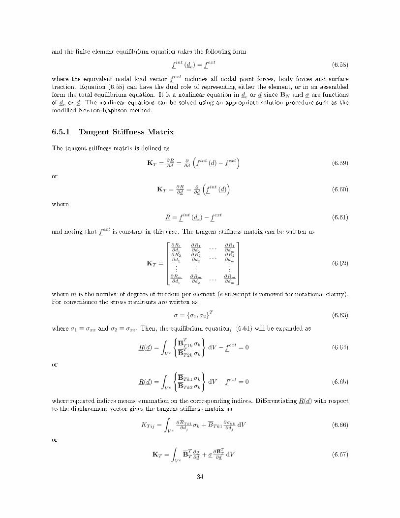
and the �nite element equilibrium equation takes the following form
f int (de) = fext (6.58)
where the equivalent nodal load vector fext includes all nodal point forces, body forces and surfacetraction. Equation (6.58) can have the dual role of representing either the element, or in an assembledform the total equilibrium equation. It is a nonlinear equation in de or d since BN and ¾ are functionsof de or d. The nonlinear equations can be solved using an appropriate solution procedure such as themodi�ed Newton-Raphson method.
6.5.1 Tangent Sti�ness Matrix
The tangent sti�ness matrix is de�ned as
KT = ∂R∂d = ∂
∂d
(f int (d)− fext
)(6.59)
or
KT = ∂R∂d = ∂
∂d
(f int (d)
)(6.60)
where
R = f int (de)− fext (6.61)
and noting that fext is constant in this case. The tangent sti�ness matrix can be written as
KT =
⎡⎢⎢⎢⎢⎢⎣
∂R1
∂d1
∂R1
∂d2. . . ∂R1
∂dm∂R2
∂d1
∂R2
∂d2. . . ∂R2
∂dm......
...∂Rm
∂d1
∂Rm
∂d2. . . ∂Rm
∂dm
⎤⎥⎥⎥⎥⎥⎦
(6.62)
where m is the number of degrees of freedom per element (e subscript is removed for notational clarity).For convenience the stress resultants are written as
¾ = {¾1, ¾2}T (6.63)
where ¾1 ≡ ¾xx and ¾2 ≡ ¾xz. Then, the equilibrium equation, (6.61) will be expanded as
R(d) =
∫
V e
{B
T
T1k ¾k
BT
T2k ¾k
}dV − fext = 0 (6.64)
or
R(d) =
∫
V e
{BTk1 ¾k
BTk2 ¾k
}dV − fext = 0 (6.65)
where repeated indices means summation on the corresponding indices. Di�erentiating R(d) with respectto the displacement vector gives the tangent sti�ness matrix as
KTij =
∫
V e
∂BTk1
∂dj¾k +BTk1
∂¾kk
∂djdV (6.66)
or
KT =
∫
V e
BT
T∂¾∂d + ¾
∂BTT
∂d dV (6.67)
34

Therefore, the tangent sti�ness matrix can be cast as
KT =
∫
V e
BT
T∇(¾) + ΞBT dV (6.68)
where
∇(¾) =
[∂¾1
∂d1
∂¾1
∂d2. . . ∂¾1
∂dm∂¾2
∂d1
∂¾2
∂d2. . . ∂¾2
∂dm
](6.69)
and
Ξ =
⎡⎢⎢⎢⎢⎢⎣
¾1∂
∂d1¾2
∂∂d1
¾1∂
∂d2¾2
∂∂d2......
¾1∂
∂dm¾2
∂∂dm
⎤⎥⎥⎥⎥⎥⎦
(6.70)
Presenting stress-strain relation as
¾ = D² (6.71)
or
¾ = DBTd (6.72)
It could be readily seen that
∇(¾) = DBT (6.73)
Substituting this result into the �rst term inside the integral, (6.68), and making use of (6.44) yields
KT =
∫
V e
BT
TDBT dV (6.74)
=
∫
V e
(BL +BN )TD (BL +BN ) dV (6.75)
=
∫
V e
BTLDBL dV +
∫
V e
BTLDBN +BT
NDBL +1
2BT
NDBN dV (6.76)
= KL +KN (6.77)
As a result, the linear part of the sti�ness matrix, KL, has been separated from the nonlinear part, KN
which makes further manipulations easier. There is one term left in (6.68), to be evaluated . The initialstress matrix, K¾, is de�ned as
KS =
∫
V e
ΞBT dV (6.78)
Considering the fact that BL is not a function of de, it follows that
ΞBL = 0 (6.79)
35

and
KS =
∫
V e
ΞBN dV (6.80)
=
∫
V e
ΞB′NN
′dV (6.81)
=
∫
V e
⎡⎢⎢⎢⎢⎢⎣
¾1∂
∂d1¾2
∂∂d1
¾1∂
∂d2¾2
∂∂d2......
¾1∂
∂dm¾2
∂∂dm
⎤⎥⎥⎥⎥⎥⎦
[1·2
∂w∂x0
]N
′dV (6.82)
=
∫
V e
⎡⎢⎢⎢⎢⎢⎣
¾1
·2∂
∂d1
∂w∂d1
¾1
·2∂
∂d2
∂w∂d1...
¾1
·2∂
∂dm
∂w∂d1
⎤⎥⎥⎥⎥⎥⎦N
′dV (6.83)
Note that for straight beams · = 1. From discretization
w = NIwI (6.84)
then,∂w∂x = wI
∂NI
∂x (6.85)
so,∂
∂dJ
∂w∂x = ±JI
∂NI
∂x
= ∂NJ
∂x (6.86)
This leads the initial stress matrix to take the following form
K¾ =
∫
V e
⎡⎢⎢⎢⎢⎢⎢⎢⎢⎢⎢⎣
0¾1
·2∂N1
∂x0...0
¾1
·2∂Nm
∂x0
⎤⎥⎥⎥⎥⎥⎥⎥⎥⎥⎥⎦
N′dV (6.87)
=
∫
V e
N′T ¾1
·2N
′dV (6.88)
(6.89)
Notice that dV = ·dz dy dx, where · is the Lamé coe�cient. The corresponding equation for straightbeams is recovered replacing ® = 1, ½ = 0 and thus · = 1. The stress vector is expressed as
{¾1
¾2
}= D
(BL +
1
2BN
)de
= D
⎡⎣
2∑
i=0
(B
′LiN+
1
2B
′NiN
′)zi
⎤⎦ de (6.90)
36

Substituting (6.90) in (6.89), and considering the appropriate form of the constitutive matrix in order tocalculate the axial stress and replacing dV by ·dz dy dx and taking the following relations into accountthe initial stress matrix can be integrated using an appropriate numerical scheme.
Ayz =
∫ ∫dy dz (6.91)
zAyz =
∫ ∫z dy dz (6.92)
Iyy =
∫ ∫z2 dy dz (6.93)
where Ayz is the area of the cross-section of the beam, z is the distance between centroid and the referenceline which is zero in this case, and Iyy is the second moment of inertia of the cross-section. It must benoted that the higher order z terms are truncated in order to be consistent with the truncation of thebinomial expansion of the Lamé coe�cient.The linear and nonlinear sti�ness matrices are computed in the same way as the initial stress matrix. Here,the linear sti�ness matrix is calculated. Recall the linear sti�ness matrix from (6.77), and substitute 6.90in the matrix gives
KL =
∫ ∫ ∫ ⎛⎝
2∑
i=0
B′LiNzi
⎞⎠
T
D
⎛⎝
2∑
i=0
B′LiNzi
⎞⎠· dz dy dx
=
∫ ∫ ∫ (B
′L0N+B
′L1Nz +B
′L2Nz2
)T
D
(B
′L0N+B
′L1Nz +B
′L2Nz2
)® (1 + ½ z) dz dy dx (6.94)
Upon expansion and neglecting higher order z terms, the linear sti�ness matrix becomes
KL = ®
∫ [Ayz
(B
′L0N)T
D(B
′L0N)+ Iyy
(B
′L0N)T
D(B
′L2N)
+ Iyy
(B
′L1N)T
D(B
′L1N)+ Iyy
(B
′L2N)T
D(B
′L0N)
+ ½
(Iyy
(B
′L0N)T
D(B
′L1N)+ Iyy
(B
′L1N)T
D(B
′L0N))]
dx (6.95)
The nonlinear sti�ness matrix can be computed in exactly the same way as the linear one.
6.6 Reduced Numerical Integration
As previously mentioned, Sec. 6.2, using Lagrange polynomials of the same orders makes the elementsusceptible to shear or membrane locking, see Appendix B. In order to avoid this problem several reducedorder integration schemes are used namely reduced shear integration, reduced membrane integration andfully reduced integration. If n is the degree of complete polynomials in an element's basis functions,Gauss integration with n+1 or more points in each direction is full and Gauss integration with n pointsor less in each direction is reduced.It is worthy to note that di�erent terms in the general expression for the sti�ness matrix K can beintegrated using di�erent integration formulae. Performing integration with di�erent schemes for di�erentterms in the sti�ness matrix is called selective reduced integration (SRI). An advantage of the SRI is thatit retains the correct rank of K.
37

When both the membrane and shear contributions are integrated with a reduced formula, the practiceis referred to as fully reduced integration. The bene�t here is the reduction in computational e�ortsrequired for calculating K since the number of quadrature points is directly changing the computationalcosts. The disadvantage of uniform reduced integration is that the rank of K may be reduced, resultingin the singularity or near singularity of the global sti�ness matrix.For integrating trigonometric basis functions several methods could be employed. Here, a compositetrapezoidal rule with a very large number of �nite intervals has been chosen. The composite trapezoidalrule is given by [2]
∫ b
a
f(x) dx = T (ℎ) +RT , T (ℎ) =ℎ
2(f0 + fℎ) + ℎ
n−1∑
i=2
fi (6.96)
The global truncation error is
RT = −ℎ3
12
n−1∑
i=0
f′′(³i) = − 1
12(b− a)ℎ2f
′′(»), » ∈ [a, b] (6.97)
Note that
x0 = a, xi = x0 + iℎ, xn = b (6.98)
where ℎ = (b− a)/n is the step length.
38

Chapter 7
Results
Two cantilever beams are considered with tip loads. The beams are loaded by a point load at the freeend of the beam. The displacement vectors are computed and compared with the available analyticalsolutions. Additionally, a comparison between di�erent Lagrange polynomials with trigonometric basisfunctions is made. The e�ects of reduced integration is also investigated. Finally, a comparison is madebetween the linear and nonlinear �nite element analysis. The main �les of the corresponding source codecan be found in A.4.
7.1 Cantilever with vertical tip load
The vertical tip de�ection of a cantilever of length L under a vertical tip load P is
wmax =PL3
3EI
(1 +
3EI
kGAL2
)(7.1)
where w is the transverse displacement, E and G are the Young's and shear modulus, I is the secondmoment of inertia of the cross-section, A is the cross-section area and k is the shear correction factor,Fig. 7.1. A series of cantilever beams with di�erent length, L, to depth, ℎ, ratios have been considered,L/ℎ ∈ {4, 10, 50}. The material and geometric input data are summarized in Table 7.1.The results of �nite element analysis of straight cantilever beams under Timoshenko assumptions forL/ℎ = 4 using di�erent types of Lagrangian basis functions along with trigonometric basis functionsis illustrated in Fig. 7.2. Both full and reduced integration schemes have been examined. As it wasexpected, cubic polynomial basis functions results in zero error, for any number of elements, regardless ofthe order of integration used, because the analytical solution for the displacement is a cubic polynomialin x. Using quadratic basis functions with the reduced shear (RS) or fully reduced (FR) integration
P
L
Figure 7.1: The cantilever straight beam.
39

Table 7.1: The material and geometric data of straight beams.Parameter Value DimensionCross-sectional area Ayz 1 in2
Second moment of inertia I 1/12 in4
Length L 4, 10, 50 inShear correction factor k 5/6 -Young's modulus E 103 psiPoisson's ratio º 1/3 -
yields exact result. While, reduced membrane integration (RM) has no such e�ect, but improves theconvergence rate.The trigonometric basis functions demonstrate higher performance than most of the Lagrangian basisfunctions. The results for trigonometric basis functions have been obtained using n = 0.25. A simplecomparison between several n values shows that n = 0.25 gives the best result in this case. All theseresults agree with the results reported in [10] and [6], except our �ndings show that using a compositetrapezoidal rule for integrating trigonometric functions results in a slower convergence in compare with [6].It should be mentioned that the relative error is de�ned as
Relative Error% = 100×∣∣∣∣∣d− d
d
∣∣∣∣∣ (7.2)
where d is an approximate value whose exact value is d. A converged result in this case means thecomputed internal energy has reached to the true internal energy.
2 4 6 8 10 12 14 16 18 20 220
10
20
30
40
50
60
70
80
90
Global Number of Nodes
Rel
ativ
e E
rror
%
Linear FLinear RSLinear RMLinear FRQuadratic FQuadratic RSQuadratic RMQuadratic FRCubicTrigonometric n = 0.25
Figure 7.2: The cantilever straight beam results, L/ℎ = 4, The relative error between the analytical andthe �nite element results for tip de�ection.
40

Similar results are presented for beams of L/ℎ = 10 and L/ℎ = 50 in Figs. 7.3 and 7.4. Results forfully integrated (F) and reduced membrane integration (RM) of the linear basis functions have beenremoved in order to present the rest of results with higher resolution. Trigonometric basis functions donot show any shear locking behaviour. The reason has been provided by Prathap and Bhashyam [10]which indicates that they can not lock. However, it must be noted that these results do not suggest that,overall, trigonometric basis functions show a higher performance than reduced shear or fully reducedintegrated polynomials in contrast with Heppler and Hansen [6], which could be due to the use of adi�erent integration scheme for trigonometric basis functions.
2 4 6 8 10 12 14 16 18 20 220
5
10
15
20
25
30
35
40
Global Number of Nodes
Rel
ativ
e E
rror
%
Linear RSLinear FRQuadratic FQuadratic RSQuadratic RMQuadratic FRCubicTrigonometric n = 0.25
Figure 7.3: The cantilever straight beam results, L/ℎ = 10, The relative error between the analytical andthe �nite element results for tip de�ection.
7.2 Quarter Circle Beam with Radial Tip Load
The next test is that of a tip loaded cantilever curved beam with a quarter of a circle arc length. Thedetails of the geometry are given in Fig. 7.5. The material properties are E = 107psi, º = 0.3 and k = 5/6.An analytical solution to this problem can be found in Lee and Sin [8] or in Young and Budynas [14] as
wmax =¼PR3
4EI+
¼PR
4kGA(7.3)
Three di�erent load condition has been considered and, for brevity, results for the radial de�ection atthe free end of the beam is shown in Fig. 7.6. Obviously, fully reduced integration scheme gives the bestresults and as it was expected the reduced membrane integration scheme results in faster convergenceand lower error in compare with reduced shear integration scheme. In curved beams membrane locking
41

2 4 6 8 10 12 14 16 18 20 220
10
20
30
40
50
60
70
80
90
100
Global Number of Nodes
Rel
ativ
e E
rro
r %
Linear RSLinear FRQuadratic FQuadratic RSQuadratic RMQuadratic FRCubicTrigonometric n = 0.25
Figure 7.4: The cantilever straight beam results, L/ℎ = 50, The relative error between the analytical andthe �nite element results for tip de�ection.
is more serious than the shear locking therefore these results agrees with the theoretical predictions, seeAppendix B.In order to examine the p-convergence of the results for tangential and radial displacements the degreesof the basis functions polynomials have been increased from 1 to 10. The results , Fig. 7.7, show a veryfast convergence in compare with h-convergence as it was expected from theory. A full integration schemehas been used to monitor the worst case from previous simulations. Results show the convergence whena 4tℎ-degree polynomial basis functions is employed.An additional set of simulation has been performed to show the e�ects of geometric nonlinearity. Theinput force has been reduced to 0.5 and nine quadratic elements with fully reduced integration scheme,which gave a perfect solution previously, has been employed. An incremental (Euler) method has beenused where load is applied in several steps. The results are presented in Figs. 7.8 and 7.9. As it is clear,the nonlinear solution starts to diverge from the linear solution after a few increment, however the errorremains small as the correction has not yet been used.A last simulation has been performed using a combination of an Euler method with a Newton-Raphsoncorrection steps. The force-displacement curve is shown in Fig. 7.10. At two major turning pointsare identi�ed, while the solution method is probably not able to catch the true curve due to its intrinsicshortcomings in following turning points or more precisely points where tangent sti�ness becomes parallelto the displacement axis.
42
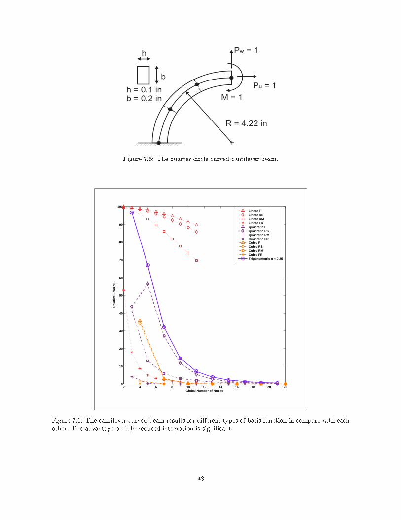
+
h
b
R = 4.22 in
h = 0.1 in
b = 0.2 in
P = 1w
P = 1u
M = 1
Figure 7.5: The quarter circle curved cantilever beam.
2 4 6 8 10 12 14 16 18 20 220
10
20
30
40
50
60
70
80
90
100
Global Number of Nodes
Rel
ativ
e E
rro
r %
Linear FLinear RSLinear RMLinear FRQuadratic FQuadratic RSQuadratic RMQuadratic FRCubic FCubic RSCubic RMCubic FRTrigonometric n = 0.25
Figure 7.6: The cantilever curved beam results for di�erent types of basis function in compare with eachother. The advantage of fully reduced integration is signi�cant.
43

1 2 3 4 5 6 7 8 9 100
10
20
30
40
50
60
70
80
90
100
Degree of Basis Functions Polynomials
Rel
ativ
e E
rro
r %
Vertical Displacement (w)Horizontal Displacement (u)
Figure 7.7: The p-convergence of the results for the cantilever curved beam. A full integration schemehas been used to monitor the worst case from previous simulations.
0 0.01 0.02 0.03 0.04 0.050
0.05
0.1
0.15
0.2
0.25
0.3
0.35
0.4
0.45
0.5
Tip deflection (in)
Fo
rce
(lb
f)
Figure 7.8: The nonlinear force-displacement curve using an incremental (Euler) method for a quartercircle beam.
44

0 0.01 0.02 0.03 0.04 0.050
2
4
6
8
10
12
Tip deflection (in)
Diff
eren
ce (
%)
with
line
ar s
olut
ion
Figure 7.9: The di�erence between nonlinear and linear solution (%).
0 0.1 0.2 0.3 0.4 0.5 0.6 0.70
0.05
0.1
0.15
0.2
0.25
0.3
0.35
0.4
0.45
0.5
Tip deflection (in)
For
ce (
lbf)
Figure 7.10: The force-displacement curve implementing a combined Euler and Newton-Raphson meth-ods.
7.3 Discussion
In full analysis of geometric nonlinearities an incremental method does not give an accountable resultsexcept in case of weak nonlinearities. Although, it is necessary to compare the method with an availablenonlinear solution to the problem. When considering the available solutions the solution has convergedto the solution. The Newton-Raphson is not promising in nonlinear analysis especially when turningand bifurcation points are present in the true response of the structure. It might have predicted thewrong results and have given an incorrect force-displacement curve. That is an important defect in theNewton-Raphson or Euler method in analyzing geometric nonlinearities.
45

Chapter 8
Conclusions
8.1 Conclusions
An important geometric nonlinearity which is still under investigation in various problems of structuralmechanics has been examined. Timoshenko beam analysis has been considered to be the one dimensionalversion of the Reissner-Mindlin plate theory, and a nonlinear form of the strain-displacement relationhas been explored. A method previously introduced by other researchers has been followed to derive thestrain-displacement relations, where the linear and nonlinear parts have been divided apart. The linear,nonlinear and stress sti�ness matrices have been derived and convergence of the method has been tested incase of available analytical solutions. The locking phenomenon has been fully investigated and the e�ectsof using reduced integration schemes have been demonstrated. The trigonometric shape functions hasshown to be able to catch the true results, although lack of an exact integration schemes is clearly seen.Fully reduced Lagrangian basis functions show the best performance, while trigonometric basis functionsdo not lock. In full nonlinear analysis, Euler method could follow the force-displacement path for verysmall loads. Combining Newton-Raphson method to the Euler method have made the method able tofollow the force-displacement path in severer cases, although it should be veri�ed with an appropriateanalytical solution.
8.2 Future Works
The possible future works are summarized here as:� It would be a good work to collect all available basis functions for beam analysis and compare their
performance when using them in �nite element analysis of Euler-Bernoulli or Timoshenko beams.� Computation time has not been considered, while it should be taken into account in order to choose
an appropriate shape function if the computational cost is of importance.� The methods presented here in formulating Timoshenko beams could be developed to some other
problems in structural mechanics.� Comparing Timoshenko beams with Euler-Bernoulli beams in nonlinear analysis could be done in
future.� In full nonlinear analysis other methods should be considered as the current method is not stable
and not able to follow the true path adequately.� Implementing Arc-length method and general displacement control methods could resolve the issues.
46

Appendix A
Source codes
The main �les are attached here, however the full versions of the source codes should be found in thecompanion CD.
A.1 Quadrilateral Bilinear Element
1 %−−−−−−−−−−−−−−−−−−−−−−−−−%2 % S.Amir Mousavi−Lajimi %3 % Copyright l’ 2009 %4 %−−−−−−−−−−−−−−−−−−−−−−−−−%5 % This code is deveoloped to calculate displacement and force vectors for6 % a plane stress problem explained in the report7 % Element : Isoparametric Quadrilateral Bilinear Element8 % The driver file is : TwoD4NIsoQuad.m9 clear all;
10 close all;11 % Include Global variables12 Vars2D4NIQ;13 % Include Input variables14 Input2D4NIQ;1516 for e=1:nele17 % Calculate the element stiffness matrix 8*818 Ke = ElementStiffness(Cmat,ngpoints,e,xI,yI);19 Kg = Assembly(Ke,e);20 K = Kg + K; % save assembled matrix21 end2223 Pf = zeros(gnodes*2,1) ;24 Pforce = [9,7.5,0;18,7.5,0] ;25 for i=1:size(Pforce(:,1))26 nnum = Pforce(i,1) ;27 v = [2*nnum−1,2*nnum];28 if any(Pf(v)∕=0)29 error('Loads matrix specifies the same entry of force twice');30 end31 Pf(v)= Pforce(i,2:3)' ;32 end33 % Apply displacement boundary conditions34 [Kbc,fbc,srow] = BCs(K,Pf,dbc);3536 % Extract displacement vectors
47

37 d1 = Kbc \ fbc;3839 % Postprocess40 [d,F]=Postprocess(d1,srow,dbc,K);
1 % Calculates the element stiffness matrix2 function Ke = ElementStiffness(Cmat,ngpoints,e,xI,yI)3 Vars2D4NIQ;4 Ke = zeros(neqe,neqe);5 [qweights,qpoints] = GaussQuad(ngpoints);67 for i=1:length(qweights)8 for j=1:length(qweights)9 [BNe,detJe] = PNmat2D4NIQ(qpoints(j),qpoints(i),xI(e,:),yI(e,:));
10 Ke = qweights(j)* qweights(i)* (BNe)' * Cmat * (BNe)* detJe*t + Ke;11 end12 end1314 end
1 %−−−−−−− calculates the derivatives of shape functions −−−−−−−−−−−−−−−−−−−%2 function [BNe,detJe,dNdr,dNds,JeInv] = PNmat2D4NIQ(r,s,x,y)3 Vars2D4NIQ;4 Ne1r = −(1/4)*(1−s) ;5 Ne2r = (1/4)*(1−s) ;6 Ne3r = (1/4)*(1+s) ;7 Ne4r = −(1/4)*(1+s) ;8 dNdr =[Ne1r;Ne2r;Ne3r;Ne4r];9 Ne1s = −(1/4)*(1−r) ;
10 Ne2s = −(1/4)*(1+r);11 Ne3s = (1/4)*(1+r) ;12 Ne4s = (1/4)*(1−r) ;dNds =[Ne1s;Ne2s;Ne3s;Ne4s];13 PNe = zeros(3,neqe);14 PNe = [Ne1r,0,Ne2r,0,Ne3r,0,Ne4r,0;15 0,Ne1s,0,Ne2s,0,Ne3s,0,Ne4s;16 Ne1s,Ne1r,Ne2s,Ne2r,Ne3s,Ne3r,Ne4s,Ne4r];17 Je = zeros(2,2);18 j = 1;19 k = 1;20 p = 1;21 for I = 1:4;22 Je(j,k) = x(I)* PNe(j,p) + Je(j,k);23 Je(j+1,k) = x(I)* PNe(j+1,p+1) + Je(j+1,k);24 Je(j,k+1) = y(I)* PNe(j,p) + Je(j,k+1);25 Je(j+1,k+1) = y(I)* PNe(j+1,p+1) + Je(j+1,k+1);26 p = p + 2;27 end28 detJe = det(Je) ;29 JeInv = inv(Je) ;30 BNe = zeros(3,8) ;31 BNe1 = zeros(3,2,4) ;3233 for I=1:434 BNe1(:,:,I) = [JeInv(1,1)*dNdr(I)+JeInv(1,2)*dNds(I),0;35 0,JeInv(2,1)*dNdr(I)+JeInv(2,2)*dNds(I);36 JeInv(2,1)*dNdr(I)+JeInv(2,2)*dNds(I),JeInv(1,1)*dNdr(I)+JeInv(1,2)*dNds(I)];37 end3839 BNe = [BNe1(:,:,1),BNe1(:,:,2),BNe1(:,:,3),BNe1(:,:,4)];40 end
48

A.2 Quadratic Triangular Element
1 %−−−−−−−−−−−−−−−−−−−−−−−−−%2 % S.Amir Mousavi−Lajimi %3 % Copyright l’ 2009 %4 %−−−−−−−−−−−−−−−−−−−−−−−−−%5 % Computes the global displacements and force vectors6 % Element : Quadratic Triangular Element78 clear all;9 close all;
10 % Input data11 Input ;12 for e=1:nele13 Ke = ElementStiffness(Cmat,ngpoints,e,XI,YI);14 K = Assembly(Ke,e) + K;15 end1617 % Apply displacement boundary conditions18 [Kbc,fbc,krow,dbc] = BCs(K,Pf);19 % Extract displacement vectors20 d1 = Kbc \ fbc;21 % Postprocess22 [F,d] = Postprocess(K,d1,krow,dbc);
1 %−−−−−−−−−−−−−−−−−−−−−−−−−%2 % S.Amir Mousavi−Lajimi %3 % Copyright l’ 2009 %4 %−−−−−−−−−−−−−−−−−−−−−−−−−%5 % Calculate the element stiffness matrix6 function Ke = ElementStiffness(Cmat,ngpoints,e,XI,YI)7 % Include Global variables8 Vars2D6NT;9 Ke = zeros(neqe,neqe);
10 [qweights,qpoints] = GaussTri(ngpoints);1112 for i=1:length(qweights)13 [dNe] = dN2D6NT(qpoints(i,1),qpoints(i,2),qpoints(i,3)) ;14 [BNe,detJe] = Bmatrices(dNe,XI(e,:),YI(e,:)) ;15 Ke = qweights(i)*BNe'*Cmat*BNe*(detJe/2)*t + Ke ;16 end17 end
1 % Computes the gradients of shape functions : B2 function [BNe,detJe] = Bmatrices(dNe,xI,yI)3 % Include Global variables4 Vars2D6NT;5 % Initialize the Jacobian6 Jx1=0;7 Jx2=0;8 Jx3=0;9 Jy1=0;
10 Jy2=0;11 Jy3=0;12 for i=1:613 Jx1 = dNe(i,1)*xI(i)+Jx1;14 Jx2 = dNe(i,2)*xI(i)+Jx2;15 Jx3 = dNe(i,3)*xI(i)+Jx3;16 Jy1 = dNe(i,1)*yI(i)+Jy1;17 Jy2 = dNe(i,2)*yI(i)+Jy2;
49

18 Jy3 = dNe(i,3)*yI(i)+Jy3;19 end20 Je = zeros(3,3);21 Je = [1 ,1 ,1 ;22 Jx1 ,Jx2 ,Jx3 ;23 Jy1 ,Jy2 ,Jy3 ];2425 detJe = det(Je);26 dLdxy = inv(Je)*[0,0;1,0;0,1];2728 dNdx = zeros(6);29 dNdy = zeros(6);30 for I=1:631 dNdx(I) = dNe(I,1)*dLdxy(1,1)+dNe(I,2)*dLdxy(2,1)+dNe(I,3)*dLdxy(3,1);32 dNdy(I) = dNe(I,1)*dLdxy(1,2)+dNe(I,2)*dLdxy(2,2)+dNe(I,3)*dLdxy(3,2);33 end34 % Initialize BNe35 BNe1 = zeros(3,2,6);36 BNe = zeros(3,12);37 for I=1:638 BNe1(:,:,I) = [dNdx(I),0;39 0,dNdy(I);40 dNdy(I),dNdx(I)];41 end42 BNe = [BNe1(:,:,1),BNe1(:,:,2),BNe1(:,:,3),BNe1(:,:,4),BNe1(:,:,5),BNe1(:,:,6)];43 end
A.3 Linear Tetrahedral Element
1 %−−−−−−−−−−−−−−−−−−−−−−−−−%2 % S.Amir Mousavi−Lajimi %3 % Copyright l’ 2009 %4 %−−−−−−−−−−−−−−−−−−−−−−−−−%5 % Computes the global displacement and force vectors6 % Computes the element displacement vectors and stresses7 % Element : Linear Tetrahedral Element8 clear all;9 close all;
10 % Include all variables11 Vars3D4NLinT;12 % Call input file13 Input;1415 for e=1:nele16 % element stiffness matrix17 Ke = ElementStiffness(Cmat,e);18 % Assemble global stiffness matrix19 Kg = Assembly(Ke,e);20 % Save global stiffness matrix21 K = Kg + K;22 end2324 % Compute and assemble point forces25 Pf = Pforces;26 % Apply displacement boundary conditions27 [Kbc,fbc,krow] = BCs(K,Pf);28 % Extract displacement vectors29 d1 = Kbc \ fbc;30 % Postprocess31 [F,d,de,Fe,sigma] = Postprocess(K,d1,krow,BmNe);
50

1 % Calculates the element stiffness matrix2 function Ke = ElementStiffness(Cmat,e)3 % Include Global variables4 Vars3D4NLinT;5 Ke = zeros(neqe,neqe) ;6 % Calculate the derivate of shape functions and Jacobian7 [detJe,dNdx,dNdy,dNdz] = dN3D4NLinT(XI,YI,ZI,e);8 BNe = Bmatrices(dNdx,dNdy,dNdz) ;9 Ke = BNe' * Cmat * BNe * Vol(e) + Ke ;
1011 end
1 % Computes the gradient of shape functions B2 function BNe = Bmatrices(dNdx,dNdy,dNdz)3 % Include Global variables4 Vars3D4NLinT;5 % Initialize BNe6 BNe1 = zeros(6,3,4);7 BNe = zeros(6,12);8 for I=1:enodes9 BNe1(:,:,I) = [dNdx(I) ,0 ,0 ;
10 0 ,dNdy(I) ,0 ;11 0 ,0 ,dNdz(I) ;12 dNdy(I) ,dNdx(I) ,0 ;13 0 ,dNdz(I) ,dNdy(I) ;14 dNdz(I) ,0 ,dNdx(I)];15 end16 BNe = [BNe1(:,:,1),BNe1(:,:,2),BNe1(:,:,3),BNe1(:,:,4)];17 BmNe(:,:,e) = BNe;18 end
A.4 Nonlinear Timoshenko Beam Analysis
1 %−−−−−−−−−−−−−−−−−−−−−−−−−%2 % S.Amir Mousavi−Lajimi %3 % Copyright l’ 2009 %4 %−−−−−−−−−−−−−−−−−−−−−−−−−%5 % The master .m file6 % TIMOSHENKO BEAM7 % NON/LINEAR FEA8 close all;9 clear all;
1011 % Input the geometric and material parameters12 InputTBFEA;1314 % Discretize the domain and define the essential boundary conditions15 MeshTBFEA;1617 % Initialize the matrices and vectors18 InitializeTBFEA;1920 % Choosing type of analysis, solution method and integration order21 MethodsTBFEA;2223 % Define the solution method parameters24 ParametersTBFEA;25
51

26 % master loop on force27 count = 0;28 sfe = zeros(gdof,NOINC);29 sfi = zeros(gdof,NOINC);30 sd = zeros(gdof,NOINC);31 dhat = zeros(gdof−size(e_bc(:,1)),1);32 reactions = zeros(gdof,1);33 siter(1)= 0;34 for ff=dP:dP:P35 count = count + 1 ;36 % Update external force vector37 fe = dfe + fe ; %+ reactions ;38 % Set up the stiffness matrices39 StiffnessTBFEA;40 AssemblyTBFEA;4142 % Apply boundary conditions43 [Khat,dfehat,DOFBC] = BCsTBFEA(K,dfe,gdof,e_bc);4445 % Solve the linear system for displacement variation46 dhat = linsolve(Khat,dfehat);4748 % Calculate current complete displacement including boundary conditions49 [dd,reactions] = GatherTBFEA(dhat,DOFBC,gdof,e_bc);5051 % Update global displacement vector52 d = d + dd ;53 %sd(:,count+1) = d(:);54 if NRFLAG == 155 % Implement Newton−Raphson method56 NRaphsonTBFEA;57 end58 sd(:,count+1) = d(:);5960 % Save force and displacement vectors61 sfe(:,count+1) = fe(:) + reactions(:) ;62 sfi(:,count+1) = fi(:) ;63 end6465 % Postprocessing the outputs66 PostprocessTBFEA;
1 function [BL,BN,NP,dw,J] = BmatricesTBFEA(enod,gp,x,w,alpha,rho)2 % THE LAGRANGE POLYNOMIAL IS GENERATED BASED ON THE NUMBER OF NODES PER3 % ELEMENT FOR AN ISOPARAMETRIC ELEMENT4 % xi : ELEMENT COORDINATE5 % enod : NODES PER ELEMENT6 % gp : GAUSS POINT7 % w : A VECTOR WHICH HAS THE w COMPONENT OF DISPLACEMENT VECTOR FOR AN8 % ELEMENT9 % BL : CONTAINS THE LINEAR B−MATRICES (= BPL * N)
10 % BL(:,:,1) = BL0, BL(:,:,2) = BL1, BL(:,:,3) = BL211 % BN : CONTAINS THE NONLINEAR B−MATRICES (= BPL * NP)12 % BN(:,:,1) = BN0, BL(:,:,2) = BN1, BL(:,:,3) = BN213 % N : KEEPS THE VECTOR OF SHAPE FUNCTIONS WHERE EACH COMPONENT OF THAT14 % CORRESPONDS TO A NODE IN ELEMENT15 % Nmat : THE MATRIX OF BASIS FUNCTIONS16 % J : THE JACOBIAN TRANSFORMATION17 % NP : CONTAINS THE DERIVATIVE OF THE BASIS FUNCTIONS WITH RESPECT TO THE18 % PHYSICAL COORDINATE SYSTEM (x) IN A ROW VECTOR IN SUCH A WAY THAT19 % EACH BLOCK IS LIKE : [0 dNI 0] WHERE I VARIES BETWEEN ONE AND THE20 % NUMBER OF NODES PER ELEMENT21 % rho : THE RECIPROCAL OF THE RADIUS OF CURVATURE22 % alpha: COEFFICIENT OF LAME COEFFICIENT
52

23 xi = zeros(1,enod) ;24 xi(1) = −1 ;25 xi(enod) = 1 ;26 if enod > 227 for i=2:(enod − 1)28 xi(i) = xi(1) + (i−1)*(2/(enod − 1)) ;29 end30 end31 N = zeros(1,enod) ;32 for i=1:enod33 M = 1;34 for j=1:enod35 if j∕=i36 N(i) = ((gp − xi(j))/(xi(i) − xi(j)))*M;37 M = N(i);38 end39 end40 end41 dN = zeros(1,enod) ;42 dNa = zeros(1,enod) ;4344 if enod==245 dN(1) = 1/(xi(1) − xi(2));46 dN(2) = 1/(xi(2) − xi(1));47 elseif enod>248 for i=1:enod49 dN(i) = 0;50 for j=1:enod51 %FF = 0;52 if j∕=i53 M = 1;54 for k=1:enod55 if (k∕=j)&&(k∕=i)56 dNa(i) = (1/(xi(i) − xi(j))) * ...57 ((gp − xi(k))/(xi(i) − xi(k))) * M;58 M = dNa(i)*(xi(i) − xi(j));59 end60 end61 FF = dNa(i) ;62 dN(i) = dN(i) + FF ;63 end64 end65 end66 end6768 J = 0;69 for i=1:enod70 J = x(i) * dN(i) + J;71 end7273 Nmat = zeros(3,enod*3);74 p =0;75 for i=1:376 k=1;77 for j=1:3:(enod*3)78 Nmat(i,j+p) = N(k);79 k = k + 1;80 end81 p = p + 1;82 end8384 NP = zeros(1,3*enod);85 i=1;86 for j=2:3:(3*enod)87 NP(j) = dN(i);88 i = i + 1;
53

89 end90 NP = NP*inv(J);9192 % Linear B−matrices93 BL = zeros(2,3*enod,3);94 BL0 = zeros(2,3*enod) ;95 BL1 = zeros(2,3*enod) ;96 BL2 = zeros(2,3*enod) ;97 p=0;98 for i=1:enod99100 BL0(1:2,i+p:i+p+2) =...101 [(1/alpha)*inv(J)*dN(i) , rho*N(i) , 0 ;102 −rho*N(i) , (1/alpha)*inv(J)*dN(i) , N(i) ];103104 BL1(1:2,i+p:i+p+2) =...105 [−(rho/alpha)*inv(J)*dN(i) , −(rho^2)*N(i) , (1/alpha)*inv(J)*dN(i) ;106 (rho^2)*N(i) , −(rho/alpha)*inv(J)*dN(i) , −rho*N(i) ];107108 BL2(1:2,i+p:i+p+2) =...109 [(rho^(2)/alpha)* inv(J) * dN(i), (rho^3)*N(i) , −(rho/alpha)*inv(J)*dN(i);110 −((rho)^(3))*N(i) , ((rho^2)/alpha)*inv(J)*dN(i), (rho^2)*N(i) ];111112 p = p + 2;113 end114 BL(:,:,1) = BL0(:,:);115 BL(:,:,2) = BL1(:,:);116 BL(:,:,3) = BL2(:,:);117118 % Nonlinear B−matrices119120 dw = 0;121 for i=1:enod122 dw = dN(i)*w(i) + dw;123 end124125 BPN0 = [(1/(alpha^2)) * inv(J) * dw ;126 0 ];127 BPN1 = [((−2*rho)/(alpha^2)) * inv(J) * dw ;128 0 ];129 BPN2 = [((3*rho^2)/(alpha^2)) * inv(J) * dw ;130 0 ];131132 BN0 = BPN0 * NP;133 BN1 = BPN1 * NP;134 BN2 = BPN2 * NP;135136 BN(:,:,1) = BN0(:,:);137 BN(:,:,2) = BN1(:,:);138 BN(:,:,3) = BN2(:,:);139140 end
1 % TIMOSHENKO BEAM2 % NON/LINEAR FEA3 % COMPUTING THE STIFFNESS MATRICES4 % ed : ELEMENT DISPLACEMENT MATRIX : edof by nele WHERE EACH COLUMN KEEPS5 % THE CORRESPONDING DISPLACEMENT VECTOR OF AN ELEMENT FOR CURRENT INCREMENT6 % ex : ELEMENT NODAL POSITION MATRIX enod by nele78 ed = zeros(edof,nele);9 ex = zeros(enod,nele);
10 for e=1:nele11 for lnID=1:enod
54

12 gnID = LG(e,lnID);13 ex(lnID,e) = Xn(gnID);14 for ldof=1:ndof15 ed(3*(lnID − 1)+ldof,e) = d(ndof*(gnID − 1) + ldof);16 end17 end18 end19 KT = zeros(edof,edof,nele);2021 for en=1:nele22 KLinear = KLinearTBFEA(D,alpha,rho,Iyy,Ayz,ex,ed,en,ngpoints,enod,edof);23 if AFLAG == 124 KNLinear = KNLinearTBFEA(D,alpha,rho,Iyy,Ayz,ex,ed,en,ngpoints,enod,edof,zb);25 end26 if AFLAG == 227 KNLinear = KNLinearTBFEA(D,alpha,rho,Iyy,Ayz,ex,ed,en,ngpoints,enod,edof,zb);28 KStress = KStressTBFEA(D,alpha,rho,Iyy,Ayz,ex,ed,en,ngpoints,enod,edof,zb) ;29 end30 KT(:,:,en) = KLinear + KNLinear + KStress;31 end
1 function KNLinear = KNLinearTBFEA(D,alpha,rho,Iyy,Ayz,ex,ed,en,ngpoints,enod,edof,zb)2 % TIMOSHENKO BEAM3 % NON/LINEAR FEA4 % COMPUTING THE NONLINEAR STIFFNESS MATRICES BOTH SHEAR AND MEMBRANE5 % CONTRIBUTIONS6 % BL : CONTAINS THE LINEAR B−MATRICES (= BPL * N)7 % BL(:,:,1) = BL0, BL(:,:,2) = BL1, BL(:,:,3) = BL28 % w : A VECTOR WHICH HAS THE w COMPONENT OF DISPLACEMENT VECTOR FOR AN9 % ELEMENT
10 % ed : ELEMENT DISPLACEMENT MATRIX : edof by nele WHERE EACH COLUMN KEEPS11 % THE CORRESPONDING DISPLACEMENT VECTOR OF AN ELEMENT FOR CURRENT INCREMENT12 % ex : ELEMENT NODAL POSITION MATRIX enod by nele13 % NA : NOT ASSIGNED (NOT USED)1415 KNLinear = zeros(edof,edof);16 KNLmembrane = zeros(edof,edof);17 KNLshear = zeros(edof,edof);18 w = ed(2:3:size(ed(:,en)),en);19 [SGW,SGP] = GaussN(ngpoints(1)) ;20 [MGW,MGP] = GaussN(ngpoints(2)) ;2122 DM = zeros(2,2);23 DM(1,1) = D(1,1) ;2425 DS = zeros(2,2);26 DS(2,2) = D(2,2) ;272829 for ip=1:size(MGP)30 [BL,BN,NA,dw,J] = BmatricesTBFEA(enod,MGP(ip),ex(:,en),w,alpha,rho);31 for iL=1:332 for iN=1:333 if (iL − 1 + iN − 1) == 034 zcoef1 = Ayz ;35 zcoef2 = zb * Ayz ;36 elseif (iL − 1 + iN − 1) == 137 zcoef1 = zb * Ayz ;38 zcoef2 = Iyy ;39 elseif (iL − 1 + iN − 1) == 240 zcoef1 = Iyy ;41 zcoef2 = 0 ;42 else43 zcoef1 = 0 ;
55

44 zcoef2 = 0 ;45 end46 KNLmembrane = alpha * (BL(:,:,iL)' * DM * BN(:,:,iN) + ...47 BN(:,:,iN)' * DM * BL(:,:,iL) + ...48 BN(:,:,iN)' * DM * BN(:,:,iN)) * zcoef1 +...49 rho * (BL(:,:,iL)' * DM * BN(:,:,iN) + ...50 BN(:,:,iN)' * DM * BL(:,:,iL) + ...51 BN(:,:,iN)' * DM * BN(:,:,iN)) * zcoef2 +...52 KNLmembrane;53 end54 end55 KNLinear = KNLmembrane * MGW(ip) + KNLinear;56 end5758 for ip=1:size(SGP)59 [BL,BN,NA,dw,J] = BmatricesTBFEA(enod,MGP(ip),ex(:,en),w,alpha,rho);60 for iL=1:361 for iN=1:362 if (iL − 1 + iN − 1) == 063 zcoef1 = Ayz ;64 zcoef2 = zb * Ayz ;65 elseif (iL − 1 + iN − 1) == 166 zcoef1 = zb * Ayz ;67 zcoef2 = Iyy ;68 elseif (iL − 1 + iN − 1) == 269 zcoef1 = Iyy ;70 zcoef2 = 0 ;71 else72 zcoef1 = 0 ;73 zcoef2 = 0 ;74 end75 KNLshear = alpha * (BL(:,:,iL)' * DS * BN(:,:,iN) + ...76 BN(:,:,iN)' * DS * BL(:,:,iL) + ...77 BN(:,:,iN)' * DS * BN(:,:,iN) ) * zcoef1 +...78 rho * (BL(:,:,iL)' * DS * BN(:,:,iN) + ...79 BN(:,:,iN)' * DS * BL(:,:,iL) + ...80 BN(:,:,iN)' * DS * BN(:,:,iN) ) * zcoef2 +...81 KNLshear;82 end83 end84 KNLinear = KNLshear * SGW(ip) + KNLinear;85 end86 KNLinear = KNLinear * J;878889 end
1 function [dd,reactions] = GatherTBFEA(dhat,DOFBC,gdof,e_bc)2 dd = zeros(gdof,1);3 reactions = zeros(gdof,1);45 for i=1:gdof6 if DOFBC(i) == 07 for p=1:size(e_bc(:,1))8 rindex = 3 * (e_bc(p,1) − 1) + e_bc(p,2);9 if i == rindex
10 dd(i) = e_bc(p,3) ;11 reactions(i) = dhat(rindex) ;12 end13 end14 elseif DOFBC(i) == 115 dd(i) = dhat(i) ;16 end17 end
56
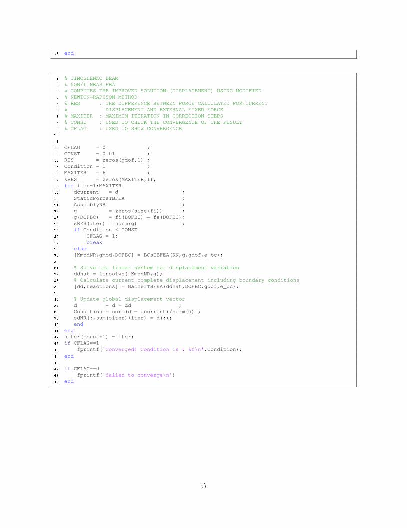
18 end
1 % TIMOSHENKO BEAM2 % NON/LINEAR FEA3 % COMPUTES THE IMPROVED SOLUTION (DISPLACEMENT) USING MODIFIED4 % NEWTON−RAPHSON METHOD5 % RES : THE DIFFERENCE BETWEEN FORCE CALCULATED FOR CURRENT6 % DISPLACEMENT AND EXTERNAL FIXED FORCE7 % MAXITER : MAXIMUM ITERATION IN CORRECTION STEPS8 % CONST : USED TO CHECK THE CONVERGENCE OF THE RESULT9 % CFLAG : USED TO SHOW CONVERGENCE
101112 CFLAG = 0 ;13 CONST = 0.01 ;14 RES = zeros(gdof,1) ;15 Condition = 1 ;16 MAXITER = 6 ;17 sRES = zeros(MAXITER,1);18 for iter=1:MAXITER19 dcurrent = d ;20 StaticForceTBFEA ;21 AssemblyNR ;22 g = zeros(size(fi)) ;23 g(DOFBC) = fi(DOFBC) − fe(DOFBC);24 sRES(iter) = norm(g) ;25 if Condition < CONST26 CFLAG = 1;27 break28 else29 [KmodNR,gmod,DOFBC] = BCsTBFEA(KN,g,gdof,e_bc);3031 % Solve the linear system for displacement variation32 ddhat = linsolve(−KmodNR,g);33 % Calculate current complete displacement including boundary conditions34 [dd,reactions] = GatherTBFEA(ddhat,DOFBC,gdof,e_bc);3536 % Update global displacement vector37 d = d + dd ;38 Condition = norm(d − dcurrent)/norm(d) ;39 sdNR(:,sum(siter)+iter) = d(:);40 end41 end42 siter(count+1) = iter;43 if CFLAG==144 fprintf('Converged! Condition is : %f\n',Condition);45 end4647 if CFLAG==048 fprintf('failed to converge\n')49 end
57

Appendix B
Locking
It has been recognized that in certain cases the predictions for displacements might be completely useless,apart from common problems with the �nite element analysis in mechanics such as inaccurate results orslow convergence. The phenomenon is characterized by a severe underestimation of the displacements, i.e.the structure is too sti� [12]. This problem is called locking referring to the intuitive understanding thatthe structure locks itself against deformations. In the main, a critical parameter plays a signi�cant rolein locking manifestation. For example, in the case of transverse shear locking of plate or beam elementsthis parameter is the slenderness of the plate or beam, and in volumetric locking it is the bulk modulus.The phenomenon can be described with the presence of some spurious stresses. These arti�cial stressesdo not appear in exact solutions of the problem. The simulated stresses augments the, arti�cial, internalenergy of the system resulting in an extra sti�ness. The aforesaid critical parameter now may lead thisenergy to inf as it approaches a large number. Therefore, the behavior of the structure is dominated bythis spurious energy, and drastic changes happen in the �nite element predictions.The shear locking occurs if the length to thickness, aspect, ratio of a beam becomes very large, that isthe beam gets very thin. Therefore, the critical parameter in the case of shear locking is the aspect ratioof the element (i.e. no property of the underlying mathematical problem itself).Shell and beam elements are susceptible to membrane locking as well. It refers to a situation wherepure bending deformations are accompanied by spurious membrane stresses. The membrane lockingonly appears if the elements are actually curved. Therefore, Quadratic elements usually show strongmembrane locking in any situation. Membrane locking can be observed in the most simple case for aquadratic (three-node) beam element. When imposing a constant bending moment it can be observedthat the membrane strains and stresses (i.e. the normal forces in the beam) are non-zero. The reasonfor the fact that the pure bending deformation cannot be represented exactly is that the exact solutionfor the displacements contains trigonometric functions which are of course not included in the shapefunctions.Several methods have been developed to overcome the problem of locking phenomenon. One simplemethod is to use a di�erent shape function for rotation which is one order lower than the one for de�ec-tion [11]. Another method is to use the same order of interpolation for both rotation and de�ection , butevaluate the energy in a proper manner such as reduced order integration. Several de�nitions are availablefor reduced order integration, such as the exactness of certain integrals, the satisfaction of certain tests,or simply evaluating the integrals using lower number of Gauss points than the required number of themfor exact integration.
58

Bibliography
[1] G. R. Cowper, �The shear coe�cient in timoshenko's beam theory,� Journal of Applied Mechanics,no. 33, pp. 335�340, 1966.
[2] G. Dahlquist and Å. Björck, Numerical Methods in Scienti�c Computing: Volume 1. Philadelphia,PA: SIAM, 2008.
[3] C. A. J. Fletcher, Computational Galerkin Methods. New York: Springer-Verlag, 1984.[4] K. K. Gupta and J. L. Meek, Finite Element Multidisciplinary Analysis, ser. AIAA Education Series.
Reston, VA: AIAA, 2000.[5] J. S. Hansen and G. R. Heppler, �A mindlin shell element which satis�es rigid body requirements,�
AIAA Journal, vol. 23, pp. 288�295, 1985.[6] G. R. Heppler and J. S. Hansen, �Performance of trigonometric basis function �nite elements in tim-
oshenko beams,� in AIAA/ASME/ASCE/AHS 28th Structures, Structural Dynamics and MaterialsConference. Monterey, California: AIAA, 1987.
[7] V. N. Kaliakin, Introduction to Approximate Solution Techniques, Numerical Modeling, and FiniteElement Methods. New York: Marcel Dekker, Inc., 2002.
[8] P. G. Lee and H. C. Sin, �Locking-free curved beam element based on curvature,� InternationalJournal for Numerical Mehtods in Engineering, vol. 37, no. 6, pp. 989�1007, 1994.
[9] A. Pica, R. D. Wood, and E. Hinton, �Finite element analysis of geometrically nonlinear platebehaviour using a mindlin formulation,� Computers & Structures, vol. 11, pp. 203�215, 1980.
[10] G. Prathap and G. R. Bhashyam, �Reduced integration and the shear-�exible beam element,� Inter-national Journal for Numerical Mehtods in Engineering, vol. 18, pp. 195�210, 1982.
[11] J. N. Reddy, An introduction to nonlinear �nite element analysis. Oxford, New York: OxfordUniversity Press, 2004.
[12] R. Wüchner, Advanced Finite Element Methods, Course Notes. Munich: Technical University ofMunich, 2009.
[13] R. D. Wood and O. C. Zienkiewicz, �Geometrically nonlinear �nite element analysis of beams, frames,arches and axisymmetric shells,� Computers & Structures, vol. 7, pp. 725�735, 1977.
[14] W. C. Young and R. Budynas, Roark's Formulas for Stress and Strain, 7th ed. New York: McGraw-Hill, 2002.
59

Index
Hamilton's Principle, 9
beam element, 31bilinear quadrilateral element, 12boundary conditions
Dirichlet, 6Neumann, 6
compatibility condition, 7compatibility equations, 7constitutive relations, 5curved beams, 29
Galerkin method, 7gauss quadrature
triangular elements, 16
Lamé coe�cient, 29linear tetrahedral element, 17locking, 58
membrane, 37shear, 37
nonlinearitiescategoris, 25geometric, 26material, 26
plane strain, 5plane stress, 5Principle of Minimum Potential Energy, 8
quadratic triangular element, 14
Reduced Numerical Integration, 37Reissner-Mindlin plate theory, 27
shear correction factor, 33solution procedures, 26
tangent sti�ness matrix, 34Timoshenko beam, 27trigonometric basis functions, 31
variational methods, 7
60


![Functionally graded Timoshenko beams with elastically ... · dynamic response of AFG-tapered Timoshenko beams. Simsek [13] investigated the buckling of Timoshenko beams composed of](https://img.dokumen.tips/doc/110x75/5e4eb76f04f2f259867e83e5/functionally-graded-timoshenko-beams-with-elastically-dynamic-response-of-afg-tapered.jpg)


