NBER WORKING PAPER SERIES

A STRUCTURAL APPROACH TO MARKET DEFINITION WITH AN APPLICATIONTO THE HOSPITAL INDUSTRY

Martin GaynorSamuel A. KleinerWilliam B. Vogt

Working Paper 16656http://www.nber.org/papers/w16656

NATIONAL BUREAU OF ECONOMIC RESEARCH1050 Massachusetts Avenue

Cambridge, MA 02138January 2011

Corresponding Author: skleiner@cornell.edu. We are grateful to Cory Capps, Rein Halbersma, R.Forrest McCluer, Barry Harris and Misja Mikkers for their comments and suggestions and Rob Jonesfor his computing assistance. All errors and opinions are the sole responsibility of the authors. Theviews expressed herein are those of the authors and do not necessarily reflect the views of the NationalBureau of Economic Research.

NBER working papers are circulated for discussion and comment purposes. They have not been peer-reviewed or been subject to the review by the NBER Board of Directors that accompanies officialNBER publications.

© 2011 by Martin Gaynor, Samuel A. Kleiner, and William B. Vogt. All rights reserved. Short sectionsof text, not to exceed two paragraphs, may be quoted without explicit permission provided that fullcredit, including © notice, is given to the source.

A Structural Approach to Market Definition With an Application to the Hospital IndustryMartin Gaynor, Samuel A. Kleiner, and William B. VogtNBER Working Paper No. 16656January 2011JEL No. I11,K21,L1,L4

ABSTRACT

Market definition is essential to merger analysis. Because no standard approach to market definitionexists, opposing parties in antitrust cases often disagree about the extent of the market. These differenceshave been particularly relevant in the hospital industry, where the courts have denied seven of eightmerger challenges since 1994, due largely to disagreements over geographic market definition. Wecompare geographic markets produced using common ad hoc methodologies to a method that directlyapplies the “SSNIP test” to hospitals in California using a structural model. Our results suggest thatpreviously employed methods overstate hospital demand elasticities by a factor of 2.4 to 3.4 and definelarger markets than would be implied by the merger guidelines’s hypothetical monopolist test. Theuse of these methods in differentiated product industries may lead to mistaken geographic market delineation,and was likely a contributing factor to the permissive legal environment for hospital mergers.

Martin GaynorHeinz CollegeCarnegie Mellon University4800 Forbes Avenue, Room 241Pittsburgh, PA 15213-3890and NBERmgaynor@cmu.edu

Samuel A. KleinerCornell UniversityCollege of Human Ecology108 Martha Van Rensselaer HallIthaca, NY 14853and NBERskleiner@cornell.edu

William B. Vogt513 Brooks HallDepartment of EconomicsTerry College of BusinessUniversity of GeorgiaAthens, GA 30602william.b.vogt@gmail.com

1

Introduction

Market definition is pivotal to the antitrust process and a key part of merger

analysis (Baker, 2007). The assessment of the potential competitive effects of a merger

or acquisition rest so heavily on the definition of a relevant antitrust market that Robert

Pitofsky, the former chairman of the Federal Trade Commission (FTC), noted that

“antitrust practitioners have long known that the most important single issue in most

enforcement actions—because so much depends on it—is market definition.” (Pitofsky,

1990, p. 1807). While there is an approximate consensus about how market definition

should be done in principle (Baker, 2007), there is wide variation in how it is

implemented in practice. A number of ad hoc methods have been used which, as we

show, do not correspond well to the agreed upon concept of an antitrust market.

Although these ad hoc methods have been widely criticized, to our knowledge they have

not been previously compared to empirical antitrust markets that are consistent with

economic theory.

It is clear that an antitrust market should be the set of products and locations that

exercise a significant competitive constraint on each other (Motta, 2004). The U.S.

antitrust authorities introduced the “SSNIP” test as a method for delineating markets

(Federal Trade Commission and U.S. Department of Justice, 1982), and this approach has

been adopted by competition authorities worldwide. The Small but Significant and Non-

transitory Increase in Price (SSNIP) test begins by defining a narrow market and asking

whether a hypothetical monopolist in the defined market could profitably implement a

SSNIP (usually a 5 percent price increase for 1 year). If sufficient numbers of consumers

are likely to switch to alternative products so as to make the price increase unprofitable,

2

then the firm or cartel lacks the power to raise price. The relevant market therefore needs

to be expanded. The next closest substitute is added and the process is repeated until the

point is reached where a hypothetical cartel or monopolist could profitably impose a 5%

price increase. The set of products/locations so defined constitutes the relevant market.

While the conceptual exercise prescribed by the SSNIP is straightforward,

implementation in practice is not. This is in part due to data limitations, and in part due

to analysts’ failure to utilize econometric analysis. If one has reliable estimates of

demand in hand, the SSNIP test can be implemented in a clear-cut way that is consistent

with the conceptual exercise. In the past, data limitations precluded demand estimation.

In addition, modern econometric methods were not brought to antitrust until

approximately 20 years ago (Scheffman and Spiller, 1987). As a consequence, ad hoc

methods of market definition were developed that did not require either extensive data or

econometric methods (Elzinga and Hogarty, 1973, 1978; Harris and Simons, 1989).

These simple quantitative approaches to market definition have been widely used

in antitrust analysis, yet have been criticized for their static nature, simplifying

assumptions and internal inconsistencies that have the potential to affect the conclusions

drawn from the use of these methods (Baker, 2007; Capps et al., 2002; Danger and Frech,

2001; Frech et al., 2004; Katz and Shapiro, 2003; Langenfeld and Li, 2001; Varkevisser

et al., 2008; Werden, 1981, 1990).

The use of such ad hoc market definition methods has been particularly influential

for antitrust decisions in the hospital industry, where 1,425 mergers and acquisitions were

successfully consummated between 1994 and 2009.1 These mergers have resulted in

1 Kaiser Family Foundation http://www.kff.org/insurance/7031/print-sec5.cfm (accessed July 16, 2010) and “Deals and Dealmakers: The Health Care M&A Year in Review” Norwalk, CT: Irving Levin Associates,

3

increases in the price of inpatient care (Keeler et al., 1999; Vita and Sacher, 2001; Capps

et al., 2003; Gaynor & Vogt, 2003; Dafny, 2009), no measurable increase in the quality

of care (Hamilton and Ho, 2000)2 and an estimated loss of $42 billion in consumer

welfare (Town et al., 2005).3 While the hospital industry has seen more merger litigation

in recent years than any other industry,4 the courts have denied all but one government

request to block hospital mergers since 1994,5 due largely to the inability of the antitrust

authorities to convincingly define a geographic market that supports their case.6 In the

eight cases brought to the courts since 1994, the primary reason given for denying the

government’s request in six of these cases centered on the markets delineation.7

This paper introduces a new method for market definition using a fully specified

structural model of consumer demand and firm behavior. The exercise prescribed by the

SSNIP can be performed exactly by using such a model. The use of these models has

Inc., 15th Edition, 2010, 14th Edition, 2009, 13th Edition, 2008, 12th Edition, 2007, http://www.levinassociates.com/compallconfirm?sid=6050 (accessed July 16, 2010). 2 The Federal Trade Commission produced evidence in the Evanston Northwestern case that a hospital merger had led to increased prices without any corresponding increase in quality (see Majoras, 2007). 3 See Town and Vogt (2006) for a recent survey on the effects of hospital consolidation. 4 Health Care Mergers and Acquisitions Handbook, Section of Antitrust Law (American Bar Association, 2003) p. 1 5 Evanston Northwestern Healthcare was decided in favor of the FTC in 2007. This case marked the first time the FTC retrospectively challenged a fully consummated hospital merger .Although the case was decided in favor of the FTC, no divestiture was mandated for the merging parties. 6 Product market definition has not been an issue in hospital merger cases, therefore all of the attention has been focused on geographic markets. 7 The eight cases brought since 1994 are Ukiah [In re Adventist Health System/West and Ukiah Adventist Hospital, 117 F.T.C. 224 (1994)], Joplin [FTC v. Freeman Hospital (1995, 911 F. Supp. 1213)], Dubuque [United States of America v. Mercy Health Services and Finley Tri-States Health Group, Inc., 902 F.Supp. 968 (1995)], Grand Rapids [Federal Trade Commission v. Butterworth Health Corporation and Blodgett Memorial Medical Center, 946 F. Supp. 1285 (1996)], Long Island [United States of America v. Long Island Jewish Medical Center and North Shore Health System, Inc., 983 F. Supp. 121 (1997)], Poplar Bluff [Federal Trade Commission v. Tenet Healthcare Corporation, 17 F. Supp. 2d 937 (1998)], Sutter [California v. Sutter Health Sys., 84 F. Supp. 2d 1057 (N.D. Cal.), aff'd mem., 2000-1 Trade Cas. (CCH) U 87,665 (9th Cir. 2000), revised, 130 F. Supp. 2d 1109 (N.D. Cal. 2001)] and Evanston [In the Matter of Evanston Northwestern Healthcare Corporation and ENH Medical Group, Inc., Initial Decision, Oct. 20, 2005, Docket No. 9315, available at http://www.ftc.gov/os/adjpro/d9315/ 051020initialdecision.pdf.]. All but U.S. v. Long Island Jewish Med. Ctr and Evanston Northwestern Health Care were lost due to failure to define a geographic market. Also, one of the cases was brought by state antitrust enforcers without either Agency's involvement. See Sutter Health Sys., 84 F. Supp. 2d 1057.

4

been promoted in the past decade as a theoretically superior approach to merger analysis

in differentiated product industries, (e.g., Motta, 2004; Baker, 2007; Geroski and Griffith,

2004; van Reenen, 2004; Ivaldi and Lőrincz, 2009) however, such an approach has not

been commonly employed in antitrust analysis. Consequently little is known about the

differences in markets produced by these methods relative to methods used in actual

cases. We apply this method to the hospital industry and compare the markets implied by

this model to those produced by the ad hoc techniques that have been used in hospital

merger cases. We seek to better understand the extent to which currently employed

methods of market definition define markets that are consistent with the criteria for

merger analysis described in the merger guidelines.

Our results suggest that the market definition techniques that have been used in

antitrust enforcement of hospital mergers by and large incorrectly define (geographic)

markets as specified by the merger guidelines’ hypothetical monopolist test. Our analysis

of a large subset of hospitals in the state of California using 1995 data suggests that

markets implied by previously employed quantitative market definition methods are, in

the majority of cases, substantially larger than those that would be implied by a method

rooted in the principles set forth in the merger guidelines. Finally, our examination of

mergers in San Diego provides an illustration of the differences in implied market

concentration in a localized region of the state, and enables comparison of our approach

to an alternative market definition method for hospitals developed by Capps et al. (2003).

Our paper proceeds as follows. Part I provides background on the merger

guidelines and their application in the hospital industry. Part II discusses quantitative

approaches to market definition. Part III outlines our use of a structural model to define

5

geographic markets. Part IV details the simulation methods used for our comparison

methodologies, while Part V describes our data. Part VI presents our main results. Part

VII concludes.

I. The Merger Guidelines and Market Definition

The Merger Guidelines

The merger guidelines are a collaborative effort by the FTC and DOJ outlining

the enforcement policy of the agencies concerning horizontal acquisitions and mergers

subject to section 7 of the Clayton Act, section 1 of the Sherman Act, or section 5 of the

FTC Act.8 They are considered to be the foremost articulation of the government’s policy

regarding enforcement standards for horizontal mergers (Werden, 1997). Their purpose

is to convey the analytical framework by which the government is to go about

determining the extent to which a merger is likely to lessen competition.

Though the first guidelines were released in 1968 and modified as recently as

2010, the thrust of the criteria for market definition was pioneered largely in the 1982

version.9 The approach to market definition in the 1982 guidelines focused on the central

enforcement-related question of whether a merger would result in a price increase

through the use of the “SSNIP” criterion. In the SSNIP criterion, an antitrust market is

defined as a group of products and a geographic area in which a hypothetical profit-

maximizing firm, not subject to price regulation, that was the only present and future

seller of those products in that area would impose a “small but significant and non-

8 Mergers subject to section 7 are prohibited if their effect “may be substantially to lessen competition, or to tend to create a monopoly.” Mergers subject to section 1 are prohibited if they constitute a “contract, combination or conspiracy in restraint of trade.” Mergers are subject to section 5 if they constitute an “unfair method of competition.” 9 The FTC joined the DOJ in releasing joint guidelines beginning in 1992.

6

transitory increase in price” (SSNIP) above all prevailing or likely future levels holding

constant the terms of sale for all products produced elsewhere. As a general matter, it

defined a price increase as significant if it was at least 5% and lasted for one year.10 The

general idea in this process is to find the smallest group of products or firms for which

there are no close substitutes, thus allowing such a hypothetical monopolist to exert

market power.11

The development of this concept was notable in that the economic reasoning was

comprehensible to both attorneys and economists, and the methodology was operable.

Though economists and attorneys still differ on the implementation aspect of market

definition analysis, the basis for these disagreements is typically methodological rather

than the fundamental theoretical question of what defines a market (Scheffman et al.,

2002). To this day the SSNIP criterion continues to be the standard by which courts

define antitrust markets.

The determination of market boundaries using the SSNIP test provides the basis

on which any subsequent steps rest when evaluating a merger. As Miles (2005) details,

10 This was later refined in 1984 to ensure that 5% was not a rule, but 5% has nonetheless remained a standard utilized in hospital merger cases by the courts. This was indicated in the Sutter case, as the court requires a basis for deviating from this prescribed 5% figure. See California v. Sutter Health Sys., 84 F. Supp. 2d 1057 (N.D. Cal.), aff'd mem., 2000-1 Trade Cas. (CCH) U 87,665 (9th Cir. 2000), revised, 130 F. Supp. 2d 1109 (N.D. Cal. 2001). 11 It should be noted that although the SSNIP test mandates that other prices be held constant, the assumption of Bertrand competition assumes that reaction functions of other firms are upward sloping in the prices of all other firms, and thus other firms would raise prices in reaction to the increase in price by a firm. For this reason, the sizes SSNIP estimates of geographic markets are most likely an upper bound. This is because upward sloping reaction functions for competitors (and thus higher prices) would induce less substitution away from the hospitals included in the SSNIP test, and thus would require a smaller number of coordinated price increases in order to increase profit. For an alternative approach that asks whether the candidates in the market would increase prices by at least 5% in equilibrium, see Ivaldi and Lőrincz (2009).

7

the court is required to follow a sequence of steps in determining the legality of a merger

consisting of12:

1. Definition of the relevant product market.

2. Definition of the relevant geographic market.

3. Identification of the competitors in the market defined from steps (1) and (2).

4. Calculation of market shares and Herfindahl-Hirschmann Index (HHI) of the

competitors in the market.

5. Calculation of merging firms’ post-merger market share and the level of post-merger

HHI. If this is too high, the merger is determined unlawful.

6. Consideration of other factors that indicate that the merger is unlikely to have

anticompetitive effects, such as ease of entry, ownership status, excess capacity and

efficiency gains.

The first two steps involved in merger analysis are pivotal to the process in each

subsequent step. The inclusion of many products will understate market concentration,

while failure to include relevant products will overstate concentration. Likewise, the

delineation of geographic markets is fundamental to the determination of the degree of

market power. The inclusion of an inappropriately large number of firms will overstate

the degree of competition, while failure to incorporate all firms involved will understate

the prevailing competitive environment.

Once the market boundaries have been set, the merger guidelines specify levels

and changes in the HHI which serve as a guide as to when mergers are likely to be anti-

competitive.13 According to the 2010 guidelines, markets with a post-merger HHI below

12 The current (2010) guidelines offer more flexibility than in the past, in that “The Agencies’ analysis need not start with market definition….although evaluation of competitive alternatives available to customers is always necessary at some point in the analysis.” (FTC/DOJ, 2010, p. 7) 13 Because the thresholds set by the guidelines are intended to be a reference point, the FTC has been flexible in their enforcement of mergers conforming to these exact HHI thresholds. See Merger Challenges

8

1,500 are said to be unconcentrated and are thus unlikely to have adverse competitive

effects. Markets with post-merger HHIs between 1,500 and 2,500 are regarded as

moderately concentrated and are likely to warrant scrutiny only if a merger will result in

an increase in the HHI of more than 100. Mergers resulting in a post-merger HHI of

above 2,500 are regarded as resulting in markets that are highly concentrated and thus

mergers producing an increase in HHI of between 100 and 200 are presumed to raise

significant competitive concerns, with increases of 200 points or more deemed likely to

enhance market power.

Application of the Merger Guidelines to Hospital Care

In the case of hospital care, the relevant product market has not been an issue of

contention in merger cases. The generally accepted product market definition has been to

“cluster” products, leading to a typical product market definition of “general acute care

hospital services.”14 In only one of the last eight cases brought by the government has

failure to convincingly define a product market been a deciding factor in a hospital

merger case. 15

The inability to convincingly define geographic markets for hospital care has,

however, been the primary determining factor in six of the government’s seven

consecutive unsuccessful merger challenges between 1994 and 1999. Table 1 presents a

Data, Fiscal Years 1999–2003, Issued by the Federal Trade Commission and the U.S. Department of Justice at http://www.ftc.gov/os/2003/12/mdp.pdf 14 Health Care Mergers and Acquisitions Handbook, Section of Antitrust Law (American Bar Association, 2003), p. 30 15 See United States of America v. Long Island Jewish Medical Center and North Shore Health System, Inc., 983 F. Supp. 121 (1997).

9

list of the most recent cases challenged by the government, as well as the size of the

geographic markets and level of concentration in each market.16

II. Quantitative Approaches to Geographic Market Definition

As discussed above, market definition is pivotal to the antitrust process. Failure to

correctly define a market may have serious consequences in antitrust cases. However,

because the merger guidelines prescribe their methodology through a thought experiment

rather than a concrete methodology, there is no uniform approach for defining these

markets. As a result, numerous quantitative approaches have been suggested and applied

across many industries including beverages, software, hospitals and supermarkets. These

include approaches based on product shipments, methodologies incorporating

econometric methods and merger simulation, and analysis of consummated mergers.17

Since we are using the hospital industry as our example, and since market definition

issues in this industry have revolved around geographic, rather than product markets, our

discussion in what follows will focus on geographic markets. It should be understood,

however, that the methodological issues are essentially the same regardless of whether

the focus is on product or geographic markets.18

Shipments-Based Approaches

16 Only a fraction of the merger activity that has occurred has been challenged due to the issuance of the Statements of Antitrust Enforcement Policy in Health Care which stipulated that mergers involving hospitals with (1) less than 100 licensed beds, (2) less than 40 daily patients over the past 3 years, (3) a merger that has been in existence for more than 5 years would not be challenged (see http://www.ftc.gov/reports/hlth3s.htm). 17 Although market definition cases rely upon quantitative methods as a basis for merger evaluation, these cases often use factual qualitative evidence as well, such as testimony from buyers of the relevant product. 18 Once can think of geographic location as a product attribute, in which case there’s no real difference between product and geographic markets.

10

Shipments-based approaches have been commonly employed for geographic

market definition analysis in industries such as beer,19 photographic film20 and

software,21 and are, to the best of our knowledge, the only quantitative approaches

employed in hospital merger cases. The two methodologies most heavily utilized,

referred to as Elzinga-Hogarty and Critical Loss Analysis, rely on discharge (shipments)

data which are usually available from the hospitals themselves or from state reporting

agencies. Because of their utilization in the vast majority of hospital merger cases, we

focus mainly on these approaches in our analysis, as our aim is to examine market

definition methodology as it has been utilized in practice. Table 2 lists the market

definition methods used in actual hospital merger cases.

Elzinga-Hogarty

The Elzinga-Hogarty method, (Elzinga and Hogarty, 1973, 1978) uses shipments

information consisting of origin and destination data for delineating a market. Although

not originally developed for use in the hospital industry, as Table 2 indicates, it has been

utilized extensively in hospital merger cases. The Elzinga-Hogarty method determines

that a geographic area constitutes a market if that area satisfies a joint ratio of import and

export thresholds. The simultaneous satisfaction of these thresholds is evidence of the

self-sufficiency of the area for both demand and supply, and is thus a geographic market.

The method argues that if an area imports little of a particular product, it can be deemed a

market from a demand perspective. By similar logic, Elzinga and Hogarty argue that if an

19 United States v. Pabst Brewing Co., (1966) 20 United States v. Eastman Kodak Co. (1995) 21 United States v. Oracle Corp., (2004)

11

area exports little of a particular product, it can be deemed a market from a supply

perspective.

While Elzinga-Hogarty has frequently been acknowledged by the courts as an

acceptable method by which to define geographic markets, there are a number of

criticisms regarding the potential shortcomings of geographic markets defined using this

methodology, with particular attention devoted to its limitations for defining hospital

markets. 22 The first centers on heterogeneity by geography in quality or service. This

issue is particularly relevant in high-service, tertiary care urban hospitals which draw

large inflows of patients from rural areas. If a sufficient number of rural patients obtain

care at the urban hospitals, the Elzinga-Hogarty test could conclude that the urban and

rural areas are in the same geographic market, even though the price of care in the rural

region does not constrain the market power of the urban hospitals. As Werden (1990)

indicates, this scenario leads to markets that are larger than would be reasonable given

the hypothetical monopolist principle put forth in the merger guidelines.

Alternatively, the use of shipments data can underestimate the size of markets. As

Werden (1981) illustrates, two firms may be close substitutes for each other but have no

cross shipments between the regions in which they are located (due to consumers

optimizing based on transportation costs). In this case Elzinga-Hogarty would

erroneously conclude that each firm and its corresponding region constitute a market,

despite the competitive constraints present due to their high cross price elasticities.

Other critical assessments of the methodology’s implications for behavior focus on its

static nature which makes consumer behavioral assumptions based on the pre-merger

22In the most recent hospital merger case (In the Matter of Evanston Northwestern Healthcare Corporation, Docket No. 9315, FTC August 2007) Elzinga himself testified that the method is not appropriate for hospital market definition.

12

rather than post-merger terms of sale, and the “silent majority” criticism of Capps et al.

(2001) which implicitly assumes that if some patients are willing to travel to a more

distant hospital to escape a price increase by the merging hospitals, other patients will do

so as well. 23

Critical Loss Analysis

Critical Loss analysis (Harris and Simons, 1989) has been widely employed in

merger analysis since its introduction in 1989 (Epstein and Rubinfeld, 2004). It seeks to

directly answer the question posed by the merger guidelines regarding the smallest set of

hospitals that would have to be included in the market to make a hypothetical price

increase of 5% profitable. Although it has been used less frequently than the Elzinga-

Hogarty methodology, Critical Loss has played an important role in determining

geographic markets in industries such as chewing tobacco24 and supermarkets,25 and in

hospital cases such as the Dubuque, Poplar Bluff and Sutter cases detailed in Table 2. In

addition, in the Poplar Bluff case mentioned above, the circuit court gave substantial

weight to the defendant’s Critical Loss analysis in its reversal of the district court’s initial

ruling (Langenfeld and Li, 2001).

The Critical Loss test proceeds in three steps. For a given set of firms, the first

step is to determine, for a given price increase, the percentage reduction in demand that

would render such a price increase unprofitable. This percentage reduction is a function

23 For a summary of the arguments and evidence against the use of shipments based methods in the context of a recent case, see “Brief of Health Care and Industrial Organization Economists as Amici Curia in Support of Petitioners,” Little Rock Cardiology Clinic PA v. Baptist Health, No. 09-1183, in the Supreme Court of the United States. http://www.scotusblog.com/wp-content/uploads/2010/06/09-1183_Amicus-brief-of-the-Health-Care-and-Industrial-Organization-Economists.pdf (accessed August 13, 2010). 24 FTC v. Swedish Match North America Inc., and National Tobacco Company, LP. 25 FTC v. Whole Foods Mkt., Inc. and Wild Oats Mkt., Inc.

13

of the proposed price increase (typically fixed at 5%) and the gross margin of the firm.

For a firm with high margins, the loss of relatively few consumers will significantly

impact profitability, while low margin firms would need to lose fewer customers in order

to impose the same impact on profitability. The second step involves calculating the

actual percentage of sales that a firm would lose were they to increase their price by a

given percentage. This is called the estimated loss. The third step entails comparing the

Critical Loss with the estimated loss. If the estimated loss is greater than the Critical

Loss, this area does not constitute a market as defined by the SSNIP test.26 The market is

then expanded to include firms that are viewed as the next closest substitutes for the

group of hospitals in question.

While the principles of Critical Loss rest upon sound economic reasoning, in

practice the implementation of Critical Loss has been subject to a number of criticisms.

One criticism concerns the classification of accounting cost data used for the

determination of the contribution margin, as the use of such data to calculate the

contribution margin allows for discretion in the classification of fixed versus variable

costs. An incentive exists for merging parties to classify a large portion of their costs as

fixed, since such classification reduces the scope of costs that can be determined as

variable, thus resulting in the determination of a high contribution margin and large

Critical Loss markets (Langenfeld and Li, 2001).

The implementation methods used in the determination of the estimated loss have

also been subject to criticism, particularly as they have been employed in hospital merger

cases. This is because in practice, determination of the estimated loss in hospital merger

26 Health Care Mergers and Acquisitions Handbook, Section of Antitrust Law (American Bar Association, 2003) p. 52-54

14

cases has entailed examining zip codes in which a significant percentage (e.g. 20% or

more) of patients already use other hospitals. It is then argued that given a price increase,

a significant number of patients in these zip codes would switch to an alternative hospital

and make such an increase unprofitable. Such claims are, however, disputed since the

high contribution margins claimed by analysts also imply that the actual loss sustained by

a firm would be small. This is because the presence of a large contribution margin

implies a low elasticity of demand and consequently, a small actual loss (Katz and

Shapiro, 2003; Danger and Frech, 2001). Furthermore, a paper by Simpson (2001)

argues that in areas deemed contestable (presumably indicating a high elasticity of

demand), price increases at nearby hospitals in actuality induce very small numbers of

patients to switch, thus indicating that demand is in fact less elastic in these contestable

zip codes than has been put forward in hospital merger cases.

III. Market Definition Using a Structural Model

Using the Structural Model for Market Definition

In what follows, we employ a structural model of market competition to

implement the SSNIP test method to define hospital markets in California. We then go

on to compare the markets obtained via the SSNIP test with those via the methods that

have been commonly employed in hospital merger cases (Elzinga-Hogarty and Critical

Loss).

15

The structural model estimates demand and supply relation parameters and builds

on the work of Baker and Bresnahan (1985), Scheffman and Spiller (1987), and Froeb

and Werden (2000). We employ a model based on Berry, Levinsohn and Pakes’s (2004)

model of differentiated product oligopoly and adapted for use in the hospital industry by

Gaynor and Vogt (2003). The model is well suited to the SSNIP criteria in that it is a

fully specified model of price and quantity determination and it allows for the calculation

of own-price and cross-price elasticities for each hospital in the data. In addition, it

allows for the determination of an initial equilibrium price and quantity for the market,

thus allowing for direct implementation of the thought experiment characterized by the

merger guidelines.

This structural model of differentiated product oligopoly models demand at the

level of an individual consumer using discrete choice techniques and micro data on

individuals. This allows demographic characteristics at the level of individual consumers

to explain hospital choice. In addition, its use of multinomial logit demand implies that

the use of the model for merger predictions will result in lower post-merger prices (and

thus larger antitrust markets) than would be produced by alternative specifications

(Crooke et al., 1999). While this section presents the basic constructs of the model, for a

full exposition, including parameter estimates, see Gaynor and Vogt (2003).

With a choice set of j (j=1,…..J) hospitals, the utility of consumer i(=1,….,N) is

assumed to be of the form:

ξ (1)

where is the hospital price, is the marginal utility of income, X are observable

consumer characteristics, observable hospital characteristics and their interactions, are

16

consumer and hospital characteristics interacted with price and are unobservable

hospital characteristics. Assuming that is an i.i.d. Weibull random variable, the

probability that consumer i attends hospital j can be written as:

∑ (2)

and the demand faced by hospital j charging price pj can be written as:

∑ (3)

where is the quantity of hospital goods consumed by consumer i.

Because equation (1) contains an unobservable term ( ) that is correlated with

price, a set of hospital fixed effects are used to absorb this source of endogeneity, as

proposed by Berry, Levinsohn and Pakes (2004). Since the use of this fixed effect

obfuscates identification of , an additional regression of these hospital fixed effects on

hospital price and other observable hospital characteristics is used to recover this

parameter. Because price is also endogenous in this additional regression, exogenous

wages and predicted quantity (using only geographic distribution and exogenous

consumer characteristics) are used as instruments for price, thus enabling recovery of ,

the marginal utility of income.

17

In this model, firms are assumed to maximize profits à la Bertrand.27 Multi-plant

firms (called multihospital systems) are also common in this industry, necessitating a

model which accounts for substitution among plants and the coordination of pricing.

Letting θ represent a J×J matrix with θjk = 1 if hospitals j and k have the same owner and

θjk = 0 otherwise, the familiar Bertrand pricing equation used in the model is of the form:

Θ⊗ Q (4)

where / is the J×J demand derivative matrix and ⊗ denotes an element-by-

element Hadamard matrix multiplication operator.

Of note for this model is that it allows for observed consumer heterogeneity via

varying distances from consumers to hospitals and thus does not exhibit independence of

irrelevant alternatives or the restrictive substitution patterns of the logit (Train, 2003).

Using the estimates obtained from this model, own-price and cross-price elasticities can

be calculated for each hospital in the dataset using the formulas:

∑ 1 (5)

∑ (6)

where (5) corresponds to the calculation of the own-price, and (6) to the cross-price

elasticity.

27 Not-for-profit firms are common in this industry. Not-for-profit hospitals are assumed to value output (e.g., community service, access to care). This makes not-for-profits, in essence, like for-profits with lower marginal costs. The econometric model allows for marginal cost (and demand) differences between for-profits and not-for-profits.

18

We present a summary of the key model characteristics in Table 3.28 Hospitals

face a downward sloping demand curve, with average own-price elasticity of -4.57 and

an average price of $4,681 for a unit of care. Additionally, as the average cross-price

elasticities in the bottom of Table 3 show, hospitals physically close to one another have

higher cross-price elasticities than do hospitals far apart. For example, the average cross-

price elasticity between a given hospital and its most proximate competitor (measured by

distance) is calculated as 0.60, while the cross-price elasticity with the fifth-closest

competitor is one-third of this magnitude. This implies that markets for hospital care are

largely local.

Adapting the Structural Model for SSNIP Market Definition

In order to define geographic markets that conform as closely as possible to the

Merger Guidelines using the structural model, we define the SSNIP test for a given

hospital as the smallest set of hospitals (inclusive of the hospitals for which we are

attempting to define a SSNIP market) for which a given price increase would be

profitable, holding constant price at all other hospitals. While a formal definition of our

SSNIP markets is included in Appendix B, intuitively, the SSNIP criterion states that for

a given hospital, j, a SSNIP market is the smallest set of hospitals for which an increase

in price at this set of hospitals (including hospital j) would increase the collective profits

in the systems of which these hospitals are members. This approach allows for the

definition of geographic markets that take into account system membership, making it

consistent with the current (2010) revision of the merger guidelines in its explicit

28 All coefficient estimates are available at http://www.rje.org/abstracts/abstracts/2003/rje.winter03.gaynor.pdf

19

treatment of firms that own multiple plants in the same geographic area.29 To illustrate

the criterion, consider 4 hospitals, A, B, C and D, and let A and B be members of the

same hospital system. Suppose hospitals A and C act as a “hypothetical monopolist” and

engage in a coordinated price increase of 5% (holding the terms of sale constant at all

other locations), resulting in a decrease in demand at both hospitals and a decrease in

profits at the combined hospital entity of A and C. Suppose, however, that B is a

sufficiently adequate substitute for care at these hospitals so that the increase in profit as

a result of the increase in demand for hospital B’s services is greater than the decrease in

profits at the combined hospital entity of A and C. Hospitals A and C would be a market

under the SSNIP criterion, as the collective profits in the systems of which these hospitals

are members has increased. Likewise, if hospital D is a close substitute for the care

rendered at A and C while hospital B is not, hospital B would see little or no increase in

demand or profits and thus hospitals A and C would not be considered a market

according to the SSNIP criterion.

In the event that a price increase at a given location results in a reduction of sales that

would be large enough such that a hypothetical monopolist would not find it profitable to

impose an increase in price, the merger guidelines suggest adding the location from

which production is the next-best substitute for production at the merging firm’s location.

Because spatial differentiation is an important attribute of hospital care, when a SSNIP is

not profitable, we include additional hospitals in order of their geographic proximity to

the location of the merging hospital(s) in question. Our algorithm for implementing

29 The 2010 merger guidelines require that a hypothetical profit-maximizing firm that was the only present or future producer of the relevant product(s) located in the region would impose at least a SSNIP from at least one location, including at least one location of one of the merging firms. They also explicitly state that a single firm may operate in a number of different geographic markets.

20

SSNIP markets using the structural Bertrand model (SSNIP Market Definition) is as

follows:

1. Begin with a hospital for which one would like to define a geographic market.

2. Find the hospital geographically closest to the hospital chosen in step 1.

3. Raise the price of only these hospitals by a given percentage (we use 5%) and

allow demand to change as a result of the price increase.

4. If the total difference in profits for the hospital system (given diversion to other

hospitals in the same system) is positive, this constitutes a market by the SSNIP

test. If it does not, we add the next hospital that is geographically closest to the

hospital in step 1.

We repeat this process until the increase in price for the chosen hospitals results in a

positive difference in profits.30

IV. Comparison Methodology for Implementing the SSNIP Test

In our implementation of market definition, we employ the two versions of the

shipments-based techniques, Elzinga-Hogarty and Critical Loss, detailed in Section II.

Specifically, we seek to compare the geographic markets defined by the SSNIP criterion

using the structural model with the markets implied by the two most commonly

employed quantitative geographic market definition techniques for hospital merger cases. 30 Note that this algorithm allows for hospitals which are close substitutes and also members of the same system to capture each others’ demand as the result of a price increase at one of the hospitals. Additionally, because the current merger guidelines require only that a SSNIP be imposed at only one location, our algorithm produces markets that are likely larger than would be implied by the current (2010) revision of the merger guidelines.

21

In what follows we describe our implementation of market definition using these

methods.

Elzinga-Hogarty Simulation

As previously described, the Elzinga-Hogarty method of geographic market

definition uses shipments information consisting of origin and destination data for

delineating a market. It specifies the use of the “little in from outside” measure (LIFO) to

determine the geographic extent of demand while the “little out from inside” measure

(LOFI) determines the geographic extent of supply. The simultaneous satisfaction of a

given threshold for each of these measures is evidence of a geographic market. The

thresholds recommended in the original article are .75 for a “weak market” and .9 for a

“strong market.” With regard to hospital care, Elzinga-Hogarty can be thought of as a

joint ratio of import and export thresholds by which to judge the self-sufficiency of a

particular market. We define the “import” of health care as an individual leaving an area

in order to be treated, and the “export” of health care as an individual from another area

(other than the one being analyzed) being treated in the relevant area. Elzinga-Hogarty

posits that if an area imports little of its health care, it can be deemed a market from the

demand perspective, as few individuals see the need to leave the area to be treated. Thus

as the import ratio, defined as

import ratiopatient outflows from area of interest into any other area

total discharges from area of interest

22

gets increasingly small, 1-(import ratio) gets increasingly large. LIFO is thus defined as

1-(import ratio).

Similarly, Elzinga-Hogarty posits that if an area exports little of its health care, it

can be deemed a market from the supply perspective. Thus as the export ratio of

healthcare defined as

export ratio=patient inflows from other areas into this area

total discharges from hospitals in this area

gets increasingly small, this is equivalent of 1-(export ratio) getting increasingly large.

LOFI is thus defined as 1-(export ratio).

There are numerous ways in which Elzinga-Hogarty markets can be calculated.

Specifically, the means by which one expands a market that does not meet the prescribed

LIFO and LOFI criteria can affect the size of the market determined for a given hospital.

Frech et al. (2004) propose six methods for expanding an Elzinga-Hogarty market based

on the geographic area from which a given hospital draws its patients. For our purposes,

we employ the method of expansion termed “contiguous search” to expand the market.

This version of Elzinga-Hogarty market definition proceeds in 3 steps: The first step in

expanding the market is to set a threshold at which the simultaneous satisfaction of this

threshold for both LIFO and LOFI constitutes a market. The contiguous search method

then proceeds by first choosing a zip code for which one would like to calculate an

Elzinga-Hogarty market. LIFO and LOFI are calculated for this zip code. If either LIFO

or LOFI is less than the prescribed threshold, one chooses the zip code that contributes

most to the minimum of LIFO and LOFI, from the universe of zip codes contiguous to

23

the zip code of interest.31 For each additional zip code, zj, that is contiguous to the

combination of zip codes already included in the service area from previous iterations, z-j,

zip code zi is added, one at a time if it satisfies (for each iteration):

max , , max ,

Zip codes continue to be added until both LIFO and LOFI equal the prescribed

threshold. For our analysis, we use the “weak market” criterion of 0.75 as our threshold.

As Frech et al. (2004) detail in their work, this method is one of the two approaches that

produce markets which are relatively compact and contiguous, and produce the most

realistic geographic markets. In addition, our choice of the weak market threshold of 0.75

rather than the strong market threshold of 0.9 is because in practice, it is virtually

impossible to obtain an Elzinga-Hogarty market for hospital care at a threshold of 0.9 for

some markets in our data, short of including most of the state.

Critical Loss Simulation

In Critical Loss analysis, for a given price increase, the percentage reduction in

demand, X, that would render a price increase unprofitable is given by Harris and Simons

(1989) as

XY

Y CM *100

31 Because of data limitations, we use a fixed radius between zip code centroids to create the universe of zip codes by which to expand the market, rather than shared zip code borders.

24

where Y is the proportion increase in price (5% in the case of the SSNIP test) and CM is

the contribution margin defined as P‐AVCP

.32 This value of X is called the “Critical Loss.”

We employ a method based on previous cases for both the estimated contribution margin

as well as the estimated actual loss. Though calculation of contribution margins is

theoretically a straightforward exercise, in practice the calculation of these margins for

hospitals in merger cases is subject to the discretion of the analyst as to the definition of

fixed cost and variable cost. Consequently, our implementation of Critical Loss utilizes

approximations of these margins based on past merger cases rather than attempting to

extrapolate the classification of costs according to merging parties. The contribution

margin assumed in these cases has ranged from 41.4% in State of California v. Sutter

Health System to 65.9% in FTC v. Tenet. 33

For our simulation of the estimated loss, we employ a method of determining the

“contestable zip codes” for a market of hospitals, meaning the collection of zip codes in

which at least a fixed percentage of the patients travel to hospitals other than those

posited as a potential market. It is then hypothesized that for these zip codes, if a given

increase in price were to be implemented, the demonstrated willingness of individuals in

these zip codes to travel outside of the proposed market for care at the present terms of

sale is evidence that a sufficient number of substitutes exist. Thus it is put forward that a

SSNIP would induce a significant number of these patients to switch to hospitals not

implementing such an increase in price. Given that our goal is to approximate Critical

Loss markets as determined by previous cases, we utilize a method similar, although not

identical, to the contestable zip code method. Whereas the contestable zip code method

32 See Harris and Simons (1989) p. 212-215 for the derivation of these formulas. 33 Langenfeld and Li (2001) p. 325-329.

25

determines the contestable zip codes and then states the number from these zip codes that

would have to leave in order to make a price increase unprofitable, we instead impose a

fixed percentage that would leave contestable zip codes for a given price increase. This

step is necessary in order to implement an algorithm to find Critical Loss markets rather

than define an arbitrary market and then hypothesize about the behavior of the patients in

this area necessary to make this area a market of a given size. Though this actual loss

number is not clearly defined and could vary greatly by case, we base our actual loss

numbers on the determination in the Sutter case that suggested that the number of patients

traveling into the proposed market that would have to switch is between one-third and

two-thirds.

Given that the court ruled in favor of the defendant, we interpret this figure to be

indicative of the court’s conclusion of the likely substitution patterns of hospital

patients.34 In our calculation of Critical Loss, we apply a contribution margin of 55%

which would determine that the Critical Loss is approximately 8.3% for a 5% increase in

price. We define zip codes as contestable if 25% or more patients travel to hospitals other

than those being defined in a hypothetical merger. Finally, we assume that of the patients

that currently receive care at one of the merging hospitals, 30% of these patients from zip

codes deemed contestable (i.e. have at least 25% outflows under the pre-merger terms of

sale) would substitute to another hospital as a result of a 5% increase in price.35

34 We do acknowledge, however that the number of patients that were determined to travel into the market accounted for only 15% of the total discharges in question. The set of contestable zip codes often does constitute a larger subset of discharges than was determined “out of the market” in the Sutter case. 35 Our algorithm works as follows:

1) Start with a hospital and the hospital closest to this hospital. 2) Find the universe of Diagnosis Related Groups (DRG) served by the hospitals chosen. 3) Find the contestable zip codes given this universe of DRGs. 4) Calculate the actual loss by assuming that 30% of the patients currently attending the hospitals of

interest in the contestable zip codes acquire their care elsewhere.

26

V. Data

We use 1995 data from California’s Office of Statewide Health Planning and

Development (OSHPD) which maintains a variety of datasets on various aspects of health

care in the state.36 Below we briefly describe each of the particular datasets we draw upon

and the criteria for selecting subsets of the data.

Discharge data

Among the items collected by OSHPD for each discharge are patient

demographics, diagnosis, treatment, an identifier for the hospital at which the patient

sought care, the patient’s zip code of residence, and charges.

Annual and Quarterly Financial data

Annual financial disclosures are submitted each fiscal year and every time a

hospital changes ownership. From these data, we use information on location of the

hospital, ownership of the hospital, type of care provided by the hospital, whether the

hospital is a teaching hospital or not, and wages. Quarterly financial disclosures are

submitted by calendar quarters, so that they are synchronized both with the discharge data

and with one another.

Selections

5) Compare the loss calculated in (4) to the critical loss figure of 8.3% of original demand. If actual

loss is greater than critical loss, we add the next closest hospital and repeat steps 1-4. If not, the set of hospitals is determined to be a market.

36 http://www.oshpd.state.ca.us/

27

For 1995, there are a total of 3.6 million patient discharges. For our analysis we

use only those discharges whose payment comes from private sources. These are

discharges in the HMO, PPO, other private, self-pay, and Blue Cross/Blue Shield

categories. This amounts to 1.47 million discharges. Our motivation in making these

choices is that for patients in these categories, some entity is making explicit choices

among hospitals, based, at least in part, on price. In the case of the various insurance

categories, insurers have discretion both over which hospitals to include in their networks

of approved providers and via any channeling of patients to less expensive hospitals.

We also eliminate patients with a DRG frequency of less than 1,000, patients with

missing values for any of the variables used in any of our analyses, patients with charges

less than $500 or greater than $500,000 and consumers with lengths of stay of zero or

greater than 30. After all the exclusions, there are 913,547 remaining observations.

Of the 593 total hospitals in the financial data, we exclude hospitals such as

psychiatric hospitals, children’s hospitals, rehabilitation hospitals, and other specialty

institutions, as well as hospitals associated with staff model HMOs. In addition we

exclude hospitals with either missing or useless quarterly financial data (some hospitals

had larger deductions from revenue than they had gross revenue, for example). We also

exclude hospitals with fewer than 100 discharges for the year. Finally, we drop hospitals

whose closest competitor (in terms of distance) is in another state. This is because our

data precludes us from observing hospitals in neighboring states which could presumably

be reasonable substitutes for those hospitals located on a state border. This leaves us with

an analysis sample of 913,547 discharges and 368 hospitals.

28

VI. Results

Statewide Analysis

In order to compare markets delineated by using the three different methodologies

described above, we define markets using Critical Loss, Elzinga-Hogarty and the SSNIP

market definition using the structural model for all hospitals in our data.

Table 4 reveals substantial differences in the markets defined by the methodologies in

both the number of hospitals in each market, as well as the degree of concentration as

defined by the HHI measures. SSNIP market definition using the structural model

determines that the median hospital operates in a market of 3 hospitals with an HHI of

3,814.37 This is well above the threshold determined by the merger guidelines as being

highly concentrated. In contrast, our version of Critical Loss concludes that the median

hospital operates in a market with 16 hospitals and an HHI of 1,194. Elzinga-Hogarty

defines markets similar to Critical Loss, with the median hospital operating in a market

with 12 other hospitals and an HHI of 1,499. Thus under the merger guidelines, both the

Critical Loss and Elzinga-Hogarty methods would find that the median hospital exists in

a market that is unconcentrated.

Many health economics studies use political boundaries to define markets, such as

Metropolitan Statistical Areas (MSA), or Health Service Areas (HSA), which are defined

based on commuting patterns and patient flows respectively (U.S. Census Bureau, 2007,

page 895; Makuc, 1991). Therefore we also examine the implications of using these

boundaries to define geographic markets. This produces the lowest concentration 37 We use available beds in our calculation of HHI by market. The correlation between beds, total discharges and total patient days and other standard measures of hospital output is above .9 for all measures.

29

measures of all market definition approaches. Using MSAs to define geographic markets

implies that the median hospital operates in a market with 18 hospitals and an HHI of

1,191, while defining geographic markets using HSAs infers that the median hospital

operates in a market with 15 other hospitals and an HHI of 1,191.

A more detailed breakdown of the hospitals by geographic area reveals a

substantial amount about the competitive environment for hospitals based upon their

location. Dividing the hospitals in the sample into hospital “density quartiles” based on

the number of hospitals within a 25-mile radius exposes the wide variation in the

methodologies’ market definition for urban and rural areas. Quartile 1 includes hospitals

with 0-5 other hospitals within a 25-mile radius, quartile 2 includes hospitals with 6-18

other hospitals within a 25-mile radius, quartile 3 includes hospitals with 19-70 other

hospitals within a 25-mile radius, while quartile 4 includes hospitals with 71-110 other

hospitals within a 25-mile radius. Figure 1 maps these hospital density quartiles while

Table 5 shows the characteristics of hospitals within these quartiles

As can be seen in Figure 1, the wide variability in the number of other hospitals

within a 25-mile radius is due to the difference in hospital density in urban and rural

areas. In particular, quartile 4 consists entirely of hospitals in Los Angeles County and

Orange County, while quartile 3 consists of hospitals from the Los Angeles (44.3%), San

Francisco-San Jose (37.5%) and San Diego (18.2%) metro areas. Quartile 1 consists of

mostly Northern California hospitals, hospitals in coastal towns and on the far outskirts of

metro areas, while quartile 2 comprises a mix of hospitals on the periphery of the 5 major

30

metro areas in California, as well as the hospitals located in the central part of the state

between San Francisco and Los Angeles.38

As would be expected, the size of the geographic markets using all three of the

methodologies indicates that markets are more concentrated in areas where there are

fewer nearby hospitals and less concentrated in areas where there are more hospitals

close by. The magnitude of the concentration difference, however, varies substantially

depending on the density quartile. In particular, in quartile 1, all methodologies indicate

that the mean level of market concentration is somewhat high, although the structural

model produces markets where the mean level of market concentration is higher than that

implied by both Elzinga-Hogarty and Critical Loss. However, in this quartile, Elzinga-

Hogarty and Critical Loss agree with SSNIP market definition on the size of the market

in 22 and 10 of the 93 cases respectively, and produce smaller markets in some cases.

This stands in contrast to quartile 3 and 4 in which neither shipments-based methodology

produces markets of comparable size to markets defined using the structural model.

As is evident from Table 5, all three of the methodologies produce markets that

include more hospitals in areas with greater hospital density. However, though the change

in the level of concentration by market is directionally equivalent, the magnitudes of the

concentration levels differ substantially. This suggests that although the shipments-based

methods are consistent in their determination that antitrust markets encompass a larger

number of hospitals in areas with greater hospital density (i.e. urban areas), the difference

in market sizes determined by these methods are substantially larger than those implied

by the structural model, and these differences are greater as the number of surrounding

38 The 5 largest Metro areas in California are Fresno, Los Angeles, Sacramento, San Diego and San Francisco.

31

hospitals increases. In Los Angeles, for example, in density quartile 4, Elzinga-Hogarty

must include an average of 50 hospitals (and over 100 zip codes) in order to produce a

market, whereas Critical Loss must include an average of 65 hospitals in order for the

loss from contestable zip codes to be sufficiently small so as to produce a market. In

contrast SSNIP market definition finds that the average hospital in this quartile operates

in a market with just 5 other hospitals. In quartile 1 on the other hand, Elzinga-Hogarty

specifies a market with an average of 7.19 hospitals and Critical Loss determines that an

average market in this quartile includes 5.8 hospitals. Market definition using the

structural model determines that in this quartile, the average hospital market consists of

just 2.78 hospitals

The bottom panel of Table 5 also reveals a great deal about the market

concentration according to the prescribed thresholds set by the merger guidelines.39

Across quartiles, both Critical Loss and Elzinga-Hogarty indicate that markets become

less concentrated as we move from quartile 1 to quartile 4. The percentage of hospitals

operating in markets with HHIs of less than 1,500 for Critical Loss increases from 8.6%

in quartile 1 to 100% in quartile 4. Likewise, for Elzinga-Hogarty, the percentage of

hospitals in markets with HHIs of less than 1,500 increases from 16.1% in quartile 1 to

100% in quartile 4. SSNIP market definition using the Bertrand model finds only five

markets with HHIs of less than 1,500 in any concentration quartile.

The number of markets considered highly concentrated (HHI greater than 2,500)

also show significant changes across concentration quartiles. The percentage of hospitals

operating in markets with HHIs of greater than 2,500 according to Critical Loss decreases

39 While the guidelines specify thresholds for post-merger market shares, the HHIs discussed below are pre-merger market shares. Nevertheless, we use them as reference points in our analysis.

32

from 68.8% in quartile 1 to 0% in quartile 4. Similarly, the Elzinga-Hogarty method

determines that 51.6% of hospitals operate in markets with an HHI of greater than 2,500

in quartile 1, while in quartile 4 no hospitals operate in a market with an HHI of such

magnitude. SSNIP market definition conversely shows all but three hospitals operating

in a market with an HHI of greater than 2,500 in quartiles 1 and 2, and just 12.5% and

48.4% of hospitals in quartiles 3 and 4 operating below the 2,500 threshold respectively.

Elasticities

The structural model allows for the calculation of the elasticity of demand for

each hospital. As shown in Table 3, the average own-price elasticity of demand for a

hospital in the sample is calculated as -4.57. Table 6 indicates that this elasticity varies

by density quartile, as the average elasticity of demand for hospitals increases (in

absolute value) from 3.55 in quartile 1 to 5.48 in quartile 4. This suggests that hospitals in

areas with more nearby competitors do in fact face stiffer competition than those with a

lower number of nearby hospitals. While this increase in own-price elasticity using the

structural model is notable in and of itself, as Table 5 indicates, both the Elzinga-Hogarty

and Critical Loss methodologies produce significantly larger markets in all density

quartiles, thus implying a much flatter demand curve for each hospital and consequently a

larger elasticity than estimated by the structural model.

Because the estimated consumer utility in equation (1) depends on price, all firm-

level elasticities are a function of the price parameter contained in the specified utility

function, . Thus, the larger elasticities produced by the two comparison methodologies

are equivalent to consumers exhibiting more price sensitive behavior, or equivalently,

33

that the value of in the utility function is of larger (absolute) magnitude than is

estimated in the structural model. Thus, if we solve for this value of that produces

markets of equivalent size to our comparison methods, we can determine the elasticities

that would be required in order to produce markets of equivalent size to those implied by

Elzinga-Hogarty and Critical Loss for a 5% price increase.40

In the top portion of Table 7, we include a summary by hospital density quartile

of the average own-price elasticity in a hospital market determined by the Elzinga-

Hogarty and Critical Loss methodologies according to the structural model. For example,

for the 93 hospital markets calculated using Elzinga-Hogarty in density quartile 1, the

average own-price elasticity as calculated using the estimated price parameter in the

structural model is -3.60. In the lower panel, we present the elasticities that would be

implied by the structural model in order to make the markets determined by Elzinga-

Hogarty and Critical Loss consistent with the price elasticity assumptions of the structural

model. For example, for the same 93 hospital markets calculated using Elzinga-Hogarty

in density quartile 1, the value of this price parameter that would make consumers

sufficiently price sensitive so as to produce an equivalent market to that determined by

Elzinga-Hogarty would imply that the average own-price elasticity in these 93 markets is

-10.10. Thus the differences in these implied elasticities demonstrate that both Elzinga-

Hogarty and Critical Loss implicitly substantially overstate the price sensitivity of

consumers with regards to hospital care. Looking across all quartiles, Table 7 shows that

Critical Loss overstates the magnitude of elasticities of a hospital in the median hospital

market by a factor ranging from 2.4 in quartile 1 to 3.4 in quartile 4, while Elzinga-

40 We solve for this value of which equates the two markets using a binary search algorithm for each market.

34

Hogarty overstates these elasticities by a factor ranging from 2.3 in quartile 3 to 2.6 in

quartile 1.

These elasticity differences also suggest that the implied markups for hospital

care using these informal methods are smaller than the markups that are assumed when

analyzing actual hospital merger cases. The commonly used Lerner Index, ,

relates elasticity to margins, implying that the determination of high margins indicates a

low elasticity of demand. In the calculation of Critical Loss, the contribution margin

defined in the previous section is equivalent to the left-hand side of a Lerner Index

(assuming constant returns to scale). Thus from our elasticity estimates in Table 7, we

can infer that the percentage markup over marginal cost implied by the Critical Loss

market size is lower than the 55% that was actually used in our definition of the Critical

Loss markets. As Table 7 indicates, even in the lowest hospital concentration quartile, the

markup for a hospital in the median hospital market using the Critical Loss methodology

is 12%, while in quartile 4, the implied markup in the market for the median hospitals is

5.4%. Although Elzinga-Hogarty in its implementation does not explicitly postulate as to

the implied markup, it suffers from similar shortcomings in that it suggests markups

ranging from 7.4%-9.9% for a hospital in the median hospital market, well below those

implied by the elasticity estimates in the structural model. Both of these findings suggest

that the market definition techniques used in previously decided merger cases are

inappropriate for hospital market definition; that is, using shipments based techniques

will by and large produce overestimates of the price elasticity of demand faced by

hospitals, thus resulting in substantially larger markets than intended in the merger

guidelines.

35

An Analysis of San Diego

To further demonstrate market definition under the SSNIP criteria, we examine

markets defined in a localized area of the state. Specifically, we perform market

definition in the San Diego area. Our selection of San Diego is strategic in that it is an

area with few geographic barriers and it contains a reasonable number of hospitals so as

to allow for methodological illustration while still being computationally feasible. It also

allows us to compare the markets defined by our structural model with those delineated

by a related, and influential, model of hospital competition developed by Capps,

Dranove, and Satterthwaite (2003) and applied to proposed consolidations in New York

State by Dranove and Sfekas (2009).

Capps et al. (2003) present a model (based on Town and Vistnes, 2001) in which

insurers bargain with hospitals and the market power of a hospital is based on the

willingness to pay (WTP) of a group of consumers for the use of that particular hospital.

This model is estimated on data from San Diego, so comparisons using this method are

restricted to that area.

A summary of the San Diego area hospitals is presented in Table 8, while a map

of the hospitals in the area is presented in Figure 2. San Diego contains hospitals that fall

into hospital density quartiles 2 and 3. The dominant systems in the area in our 1995 data

are the Scripps and Sharp systems, with each controlling 6 and 5 of the 23 hospitals

respectively. While 19 of the 23 hospitals were members of a multi-hospital system, 4 of

these hospitals, Alvarado, Harbor View, Mission Bay and Paradise Valley were owned

by corporations that controlled no other hospitals in the San Diego area. The other two

36

multi-hospital systems, University of California (UC) and Palomar Pomerado, each

controlled only two hospitals.

Table 9 presents the results of SSNIP market definition for the San Diego area for

each of our three market definition methodologies. As evidenced in Table 8, San Diego

County had a moderate degree of concentration in 1995, with a system-based HHI of

1,949.41 With the exception of Fallbrook Hospital, all methods produce a market which is

a subset of the hospitals in this county.42 Critical Loss in column one defines markets as

consisting of 13-38 hospitals, each of which comprise substantial subsections of the San

Diego area, and in the case of Fallbrook Hospital, portions of the Los Angeles Area.

Similarly, Elzinga-Hogarty market definition in column two determines that markets are

anywhere from 14-19 hospitals in size. The structural model in column three, however,

shows that SSNIP markets consist instead of small sets of no more than 4 hospitals, with

a median market size of two hospitals. This difference in methodology evidently affects

the degree of concentration implied in the San Diego area. Both of the comparison

methods produce markets with the majority of HHIs falling in the 2,000-3,000 range,

while no SSNIP market produced by the structural Bertrand model has a HHI lower than

3,000 and 18 of the 23 hospitals operate in a market with an HHI of more than 5,000.

Figure 3 illustrates the differences in markets produced by the three

methodologies, using as an example the definition of a market for Scripps Memorial

Hospital - Chula Vista (Scripps Chula Vista), a 159-bed hospital located in the southern

portion of the San Diego metropolitan area. Using the SSNIP market definition

41 This HHI measure takes into account system membership and is highly correlated (correlation of over .9) with total discharges and total patient days. 42 In order to create a critical loss market for Fallbrook Hospital, the northernmost hospital in the sample, the algorithm expands into the Southern section of the Los Angeles Metropolitan Area.

37

algorithm, Scripps Chula Vista and Community Hospital of Chula Vista, a 306-bed

hospital located in the same area represent a geographic market, with a HHI of 5,500.

Using Elzinga-Hogarty, a geographic market would include these two hospitals, as well

as 16 other facilities in the San Diego area, producing a market with an HHI of 2,228.

The market produced using Critical Loss shows a similar pattern, as a critical loss market

would include a total of 17 hospitals in the San Diego metropolitan area, implying that

Scripps Chula Vista operates in a market with an HHI of 2,692.

Comparison with the Willingness to Pay Model

The Willingness to Pay (WTP) model represents a promising method of analyzing

mergers (Capps et al., 2003; Town and Vistnes, 2001). Because both the structural

Bertrand model and WTP models are both rooted in a multinomial-logit demand

specification which includes both hospital and consumer characteristics and patient-

hospital distance, we present results from a comparison of merger simulations using the

structural Bertrand model to compare price increases implied by the WTP model (see

Appendix A for a brief overview of the WTP model).43 The main differences between

the models involves the determination of firm pricing behavior; firm conduct and price

determination are not modeled explicitly in the WTP model, rather the relationship

between WTP and hospital profits is identified using a regression of hospital profits on

WTP for each hospital. Mergers in the model are simulated by calculating the difference

in WTP for a combined entity of hospitals and the sum of the WTP for each separate

hospital in this combined entity. Using the relationship between a “unit” of WTP and

hospital profits (calculated from the regression of hospital profits on WTP), and assuming 43 Details of our estimation of the WTP model are included in appendix A.

38

no change in the cost of treatment, this difference in WTP is used to show the increase in

average revenue per patient brought about by the merger, leaving quantity unchanged.

The WTP model does not allow for market definition in a localized area where a

large hospital firm (system) controls multiple plants (hospitals). This is due to the

difficulty in allocating the willingness to pay measure across hospitals of the same system

affiliation. Consequently, we adapt the structural Bertrand model to simulate mergers

between individual hospitals, as well as individual hospital systems, thereby enabling

directly comparable merger effects for each model. For our estimates of the WTP, we

employ the same variables in our utility function as were used in Capps et al. (2003) with

minor exceptions.44 Furthermore, use of the WTP necessitates a different sample of

consumers than was used in that of Capps et al. (2003) as the original estimated WTP

utility function includes Medicare patients, indemnity patients and HMO/PPO. In order to

ensure the most direct comparison of the two methods, we include only indemnity and

HMO/PPO consumers.45

Table 10 includes the results of the mergers of 27 mergers of independent

hospitals located in the San Diego area.46,47 As Table 10 demonstrates, the two models

show merger effects on price that are virtually zero for the independent San Diego

hospitals. For the mergers in Table 10, for only one merger, that of Tri-City Hospital and

44 Instead of the “equipment intensity” variable, we use a “tech index” variable which is the sum over dummy variables for the presence of 28 technologies reported in the annual hospital financial data (such as presence of an MRI, open heart surgical suite, etc.). Also, instead of travel time, we use distance. 45 This corresponds to specification (4) in Capps et al. (2003) 46 We display the results of independent hospitals primarily because Capps et. al. do not prescribe a method of calculating WTP for markets in which a hospital system controls multiple hospitals. Thus these are the “cleanest” comparisons of the two methodologies. 47 We classify a hospital as independent for purposes of this analysis if the hospital had was not a member of a hospital system or if the hospital was owned by a corporation that controlled only one hospital in the San Diego area.

39

Fallbrook Hospital, do the methods differ on whether a merger would produce a SSNIP.

They are otherwise in agreement.

Calculation of WTP does not allow for isolation of unilateral merger effects;

rather it determines the aggregate price increase implied by a merger in a chosen market.

Thus we adjust the model to account for system membership; specifically we calculate

the WTP measure for each hospital separately and given these estimates, we can then

infer the WTP for an entire hospital system. The effect of a system merger can then be

identified using the difference in the aggregate WTP for both systems versus the WTP for

each system separately. Table 11 presents the results of the merger of 5 hospital systems

in the San Diego area.

In three of the five system mergers presented in Table 11, both models agree on

which mergers would result in a 5% increase in price.48 For the two mergers presented in

Table 11 in which the two methods do not agree, both of these mergers involve the

University of California, San Diego, a hospital which generates the largest WTP measure

of all hospitals in our data. As Capps et al. (2003) indicate in their paper, this could be

due to UCSD’s status as the only university hospital in the market. This fact, coupled

with UCSD’s service area overlap with Scripp’s Mercy Hospital (0.4 miles from UCSD)

and Sharp Memorial Hospital (3.2 miles from UCSD) in downtown San Diego most

likely accounts for the substantial increase in WTP (and thus price) induced by a merger

of UCSD with both Sharp and Scripps. In the structural Bertrand model, however, UCSD

Medical Center charges the highest price for a unit of hospital care in the San Diego

48 The correlation between the merger simulations and WTP model is 0.82. Furthermore, thought the merger simulations allow for identification of individual merger effects, in order to facilitate a direct comparison of the two methodologies, we weight the price increases produced by the structural Bertrand model’s merger simulations by the demand at each hospital (pre-merger).

40

($5,827) area while also exhibiting the highest own-price elasticity (-5.99) of San Diego

area hospitals (with the exception of Villa View Hospital). This pattern is suggestive of

the UCSD Medical Center exerting market power in its pricing of hospital services.

Consequently, while a merger of UCSD with hospital systems in the area does produce

an increase in price using the structural Bertrand model, this increase is most likely not as

large as would be the case if UCSD were not already exerting market power. To the

degree that consumers and health insurers substitute to other health care providers as a

result of the prevailing high price at UCSD Medical Center, the observed elasticity may

account for the lower price increase implied by the merger of these systems in the

structural Bertrand model.

Overall, the results of the comparisons between these two methods reveal a

notable degree of similarity for hospital merger effects in the San Diego area. Though the

models differ in their assumptions about firm conduct, given that both models identify

demand-side merger effects via the intersection of patient market shares, such a result is

not surprising.

VII. Conclusion

Market definition is essential for merger analysis, and has played a pivotal role for

antitrust decisions in the hospital industry in the past two decades. The vast majority of

hospital merger cases have utilized ad hoc methods of geographic market definition that

rely heavily upon patient shipment data, with no explicit economic model used to justify

such methods. Our use of a fully specified structural model of hospital competition

compares commonly employed geographic market definition approaches used in actual

41

hospital merger cases to geographic markets rooted in the principles set forth by the

merger guidelines. This method explicitly models consumer and producer behavior, and

also accounts for firms operating at multiple locations, as required by the 2010 merger

guidelines.

We find that the use of approaches frequently utilized in previous cases largely

overstate the size of geographic markets for hospitals, particularly in areas with greater

hospital density. In addition, these informal approaches imply elasticities ranging from

2.4-3.4 times as large as those calculated from a structural model of hospital competition.

Furthermore, our analysis of the San Diego area is consistent with those implied by the

model of Capps et al. (2003).

The results have important implications for merger analysis in both the hospital

industry and other industries involving differentiated products. They illustrate the

importance of economic modeling for defining markets, and indicate that reliance on

imprecise methods of market definition has the potential to mislead the courts as to the

appropriate extent of geographic markets. The markets presented here are most

consistent with those identified in merger cases by plaintiffs rather than by defendants, in

contrast to the court’s frequent rejection of markets alleged by the antitrust authorities.

Thus the use of such an approach should be emphasized when assessing the extent of

market power in this and other differentiated product industries.

42

References

American Bar Association, 2003. Health Care Mergers and Acquisitions Handbook. Chicago: ABA Publishing. Baker, J., 2007. Market Definition: An Analytical Overview. Antitrust Law Journal, 74, pp.129-173. Baker, J. and Bresnahan, T., 1985. The Gains From Merger or Collusion in Product-Differentiated Industries. The Journal of Industrial Economics, 33(4), pp.427-444. Berry, S., Levinsohn, J. & Pakes, A., 2004. Differentiated Products From a Combination of Micro and Macro Data: The New Car Market. Journal of Political Economy, 112(1), pp.68-105. Capps, C., & Dranove, D., 2004. Hospital Consolidation and Negotiated PPO prices. Health Affairs 23(2), pp.175-181. Capps, C., Dranove, D., Greenstein, S. & Satterthwaite, M., 2001. The Silent Majority Fallacy of the Elzinga-Hogarty Criteria: A Critique and New Approach to Analyzing Hospital Mergers. National Bureau of Economic Research Working Paper No. W8216. Capps, C., Dranove, D., & Satterthwaite, M., 2002. Antitrust Policy and Hospital Mergers: Recommendations for a New Approach. Antitrust Bulletin 47(4), pp.677-714. Capps, C., Dranove, D., & Satterthwaite, M., 2003. Competition and Market Power in Option Demand Markets. RAND Journal of Economics 34(4), pp.737-763. Crooke, P., Froeb, L., Tschantz, S. & Werden, G.J., 1999. Effects of Assumed Demand Form on Simulated Postmerger Equilibria. Review of Industrial Organization, 15(3), pp. 205 – 217. Dafny, L. 2009. Estimation & Identification of Merger Effects: An Application to Hospital Mergers. Journal of Law and Economics, 52(3), pp.523-550. Danger, K. L. & Frech, H.E. III, 2001. Critical Thinking about Critical Loss in Antitrust. Antitrust Bulletin, 46(2), pp.339-355. Dranove, D. & Sfekas, A., 2009. The Revolution in Health Care Antitrust: New Methods and Provocative Implications. The Milbank Quarterly, 87(3), pp.607–632. Duan, N., 1983. Smearing Estimate: A Nonparametric Retransformation Method. Journal of the American Statistical Association, 78(383), pp.605-610. Elzinga, K.G. & Hogarty, T.F., 1973. The Problem of Geographic Market Definition in Antimerger Suits. Antitrust Bulletin, 18(1), pp.45-81.

43

Elzinga, K, and T. Hogarty. 1978. "The Problem of Geographic Market Delineation Revisited: The Case of Coal." Antitrust Bulletin, 23 (1): 1-18. Epstein, R.J. & Rubinfeld, D.L., 2004. Effects of Mergers Involving Differentiated Products. Technical Report for Directorate-General Competition, European Commission [Online]. Available at: http://ec.europa.eu/competition/mergers/studies_reports/effects_mergers_involving_differentiated_products.pdf [Accessed 13 June 2010]. Federal Trade Commission and U.S. Department of Justice, 1992. Horizontal Merger Guidelines, (issued 1992, revised 1997), http://www.ftc.gov/bc/docs/horizmer.shtm (accessed December 7, 2010). Federal Trade Commission and U.S. Department of Justice, 2010. Horizontal Merger Guidelines, http://www.ftc.gov/os/2010/08/100819hmg.pdf (accessed December 5, 2010). Frech, H.E. III, Langenfeld, J., & McCluer, R. F., 2004. Elzinga-Hogarty Tests and Alternative Approaches for Market Share Calculations in Hospital Markets. Antitrust Law Journal 71(3), pp.921-947. Froeb, L. & Werden, G.J., 1992. The Reverse Cellophane Fallacy in Market Delineation. Review of Industrial Organization, 7(2), pp.241-247. Froeb, L.M. & Werden, G.J., 2000. An Introduction to the Symposium on the Use of Simulation in Applied Industrial Organization. International Journal of the Economics of Business, 7(2), pp.133–137. Gaynor, M. & Vogt, W.B., 2000. Antitrust and Competition in Health Care Markets. In A.J. Culyer and J.P. Newhouse, eds. Handbook of Health Economics, Vol. 1B. New York: North-Holland. Ch.27. Gaynor, M. & Vogt, W.B., 2002. Competition Among Hospitals. National Bureau of Economic Research Working Paper No. W9471. Gaynor, M. & Vogt, W.B., 2003. Competition Among Hospitals. RAND Journal of Economics, 34(4) pp.764–785. Geroski, P. and Griffith, R. 2004. Identifying anti-trust markets. International Handbook of Competition, M. Neumann and J. Weigand (eds.), Cheltenham, UK: Edward Elgar. Hamilton, B. & Ho, V., 2000. Hospital Mergers and Acquisitions: Does Market Consolidation Harm Patients? Journal of Health Economics, 19(5) pp.767-791.

44

Harris, R. & Simons J.J., 1989. Focusing Market Definition: How Much Substitution is Necessary? Research in Law and Economics, 12, pp.207-226. Hausman, J., Leonard, G. & Zona, J. D., 1994. Competitive Analysis with Differentiated Products. Annales d'Economie et de Statistique, 34, pp.159-180. Horowitz, I. 1987. Market Definition in Antitrust Analysis: A Regression-Based Approach. Southern Economic Journal, 48(1), pp.1-16. Ivaldi, M. and Lörincz, Sz. 2009. "Implementation Relevant Market Tests in Antitrust Policy: Application to Computer Servers", Review of Law and Economics, forthcoming. Katz, M., & C. Shapiro, 2003. Critical Loss: Let’s Tell the Whole Story. Antitrust, 17(2), pp.49-56. Keeler, E.B., Melnick, G., & Zwanziger, J., 1999. The Changing Effects of Competition on Non-Profit and For-Profit Hospital Pricing Behavior. Journal of Health Economics, 18(1), pp.69-86. Langenfeld J. & Li, W., 2001. Critical Loss Analysis in Evaluating Mergers. Antitrust Bulletin, 46(2), pp. 299-337. Leibenluft, R.F. Esq., 1998. Antitrust Enforcement and Hospital Mergers: A Closer Look, [Online]. Available at: http://www.ftc.gov/bc/hmerg1.htm [Accessed 8 March 2010]. Luke R.D., Ozcan Y.A. & Olden P.C., 1995. Local Markets and Systems: Hospital Consolidations in Metropolitan Areas. Health Services Research, 30(4), pp.555-75. Makuc, D., B. Haglund, D. Ingram and J. Kleinman 1991. Health Service Areas for the United States, Vital and Health Statistics, Series 2, No. 112 (National Center for Health Statistics). Majoras, D.P., 2007. “Opinion of the Commission,” In the Matter of Evanston Northwestern Healthcare Corporation, Docket No. 9315, http://www.ftc.gov/os/adjpro/d9315/070806opinion.pdf, accessed 7/6/2010. Miles, J.J., 2005. Health Care and Antitrust Law. St. Paul, MN: West Group. McCarthy, T.R. & Thomas, S. J., 2003. Geographic Market Issues in Hospital Mergers. In American Bar Association Health Care Mergers and Acquisitions Handbook. Chicago, ABA Publishing. Ch. 3. Morrisey, M.A., Sloan, F.A., & Valvona J., 1988. Defining Geographic Markets for Hospital Care. Law and Contemporary Problems, 51(2), pp.165-194.

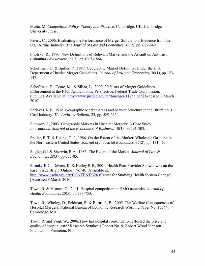
45

Motta, M. Competition Policy: Theory and Practice. Cambridge, UK: Cambridge University Press. Peters, C., 2006. Evaluating the Performance of Merger Simulation: Evidence from the U.S. Airline Industry. The Journal of Law and Economics, 49(2), pp. 627-649. Pitofsky, R., 1990. New Definitions of Relevant Market and the Assault on Antitrust. Columbia Law Review, 90(7), pp.1805-1864. Scheffman, D. & Spiller, P., 1987. Geographic Market Definition Under the U.S. Department of Justice Merger Guidelines. Journal of Law and Economics, 30(1), pp.123-147. Scheffman, D., Coate, M., & Silvia, L., 2002. 20 Years of Merger Guidelines Enforcement at the FTC: An Economic Perspective. Federal Trade Commission, [Online]. Available at: http://www.justice.gov/atr/hmerger/11255.pdf [Accessed 8 March 2010]. Shrieves, R.E., 1978. Geographic Market Areas and Market Structure in the Bituminous Coal Industry. The Antitrust Bulletin, 23, pp. 589-625. Simpson, J., 2003. Geographic Markets in Hospital Mergers: A Case Study. International Journal of the Economics of Business, 10(3), pp.291-303. Spiller, P. T. & Huang, C. J., 1986. On the Extent of the Market: Wholesale Gasoline in the Northeastern United States. Journal of Industrial Economics, 35(2), pp. 131-45. Stigler, G.J & Sherwin, R.A., 1985. The Extent of the Market. Journal of Law & Economics, 28(3), pp.555-85. Strunk, B.C., Devers, K. & Hurley R.E., 2001. Health Plan-Provider Showdowns on the Rise” Issue Brief, [Online]. No. 40. Available at: http://www.hschange.org/CONTENT/326 (Center for Studying Health System Change) [Accessed 8 March 2010]. Town, R. & Vistnes, G., 2001. Hospital competition in HMO networks. Journal of Health Economics, 20(5), pp.733-753. Town, R., Wholey, D., Feldman, R. & Burns, L. R., 2005. The Welfare Consequences of Hospital Mergers. National Bureau of Economic Research Working Paper No. 12244, Cambridge, MA. Town, R. and Vogt, W., 2006. How has hospital consolidation affected the price and quality of hospital care? Research Synthesis Report No. 9, Robert Wood Johnson Foundation, Princeton, NJ.

46

Train, K. (2003). Discrete Choice Methods with Simulation. Cambridge: Cambridge University Press. United States Census Bureau (2007). The 2007 Statistical Abstract: The National Data Book. Van Reenen, J. 2004. Is There a Market for Work Group Servers? Evaluating Market Level Demand Elasticities using Micro and Macro Models. Centre for Economic Performance, London School of Economics and Political Science, London, UK Varkevisser, M., Capps, C. S. & Schut, F.T., 2008. Defining Hospital Markets for Antitrust Enforcement: New Approaches and their Applicability to the Netherlands. Health Economics, Policy and Law, 3, pp. 7-29. Viscusi W.K., Vernon J.M. & Harrington J.E., 2000. Economics of Regulation and Antitrust. Cambridge, MA: MIT Press. Vita, M.G., & Sacher, S., 2001. The Competitive Effects of Not-for-Profit Hospital Mergers: A Case Study. Journal of Industrial Economics, 49(1) pp.63-84. Werden, G.J., 1981. The Use and Misuse of Shipments Data in Defining Geographic Markets. Antitrust Bulletin, 26(4) pp.719-737. Werden, G. J. Simulating the Effects of Differentiated Products Mergers: A Practitioners' Guide. In Caswell, J.A., and Cotterill, R.W., eds., Strategy and Policy in the Food System: Emerging Issues. Food Marketing Policy Center, Storrs, CT, 1980, pp. 95-110. Werden, G.J., 1992. The History of Antitrust Market Delineation. Marquette Law Review 76, 123-215. Werden, G., 1990. The Limited Relevance of Patient Migration Data in Market Delineation for Hospital Merger Cases. Journal of Health Economics, 8(4), pp. 363-76.

47

Appendix A: The Capps, Dranove and Sattherwaite Model of Option Demand

A.1 Consumers

Consumers are assumed to maximize ex post expected utility. Thus they maximize the

expected utility of obtaining treatment for a specific condition at a specific hospital, but

before treatment is actually obtained. The utility function is defined as

ijjiiiiijjjij pZYZYTSRUU εγ +−= ),(),,,,(

where jR is a vector of hospital characteristics that are common across all patient

conditions, jS is a vector of variables that contain patient specific service offerings, ijT

is the travel time from patient i to hospital j, iY is a vector of the patient’s socioeconomic

characteristics, and iZ is a vector of clinical attributes specific to patient i. Assuming that

),( ii ZYγ is constant, individual i will select hospital j if for all hospitals j≠k,

ijikiiikkkiiijjj ZYTSRUZYTSRU εε −>− ),,,,(),,,,( .

Assuming ε is distributed i.i.d. extreme value, the probability ijs that patient i chooses

hospital j is given as ∑∈

=

Gkiiikkk

iiijjjij ZYTSRU

ZYTSRUs

)),,,,(exp()),,,,(exp(

where G is a network of hospitals

from which the patient chooses. The the parameter estimates for our calculation of the

utility function are included in Table A.1.

The patient’s interim expected utility is thus

[ ]{ } ( )⎥⎦

⎤⎢⎣

⎡== ∑

∈∈ Gj

iiijjjiiijjjGj

IU ZYTSRUZYTSRUEV ),,,,(expln),,,,(max .

Given this result, hospital j’s contribution to individual i’s expected utility is

⎥⎥⎦

⎤

⎢⎢⎣

⎡

−=Δ

),,,(11ln),,,(

iiiijiii

IUj ZYGs

ZYGVλ

λ

48

where iλ is the location of consumer i. Capps et al. then define the ex-ante willingness to

pay for patient i as iiiZ

iii

iiiIUj dZYZf

ZYZYGV

),|(),(

),,,(λ

γλ

∫Δ

. Because this willingness to pay

is identified only up to the scale factor ),( ii ZYγ , summing over all consumers the

willingness to pay for hospital j is thus written as

iiiiiZY

iiiiij

EAj ddZdYYZf

ZYGsNGW λλ

λλ

),,(),,,(1

1ln)(,,∫

⎥⎥⎦

⎤

⎢⎢⎣

⎡

−=Δ .

A.2 Pricing

After the willingness to pay measure is calculated for hospitals, Capps et al.

regress hospital profits on the willingness to pay measure (without a constant) and

recover the coefficient from this regression, a . This generates the predicted impact of

WTP on hospital profits. Using the average revenue and average cost per discharge at a

hospital, they then calculate a measure of profits per discharge at each hospital.

A.3 Merger Effects using WTP

The first step in using WTP to simulate merger effects entails calculating the

difference in willingness to pay for a merged entity versus the willingness to pay for each

entity independently. Defining

iiiiiZY

iiiiikiiiij

EAkj ddZdYYZf

ZYGsZYGsNGW λλ

λλλ

),,(),,,(),,,(1

1ln)(,,∫

⎥⎥⎦

⎤

⎢⎢⎣

⎡

−−=Δ + ,

the increase in WTP as a result of a merger would thus be

)()()( GWGWGW EAk

EAj

EAkj Δ−Δ−Δ + .

As Capps et al. detail in their paper, if two hospitals are far enough apart, then if hospital

j has a positive market share in market segment ),,( iii YZ λ , hospital k will likely have a

49

zero market share in that same segment. Thus the expression

)()()( GWGWGW EAk

EAj

EAkj Δ−Δ−Δ + will be zero and thus a merger of hospitals j and k will

likely generate no increase in the market power of the two firms.

The second step in using WTP to simulate merger effects involves inferring the

increase in profits resulting from a merger of two firms. Capps et. al. do this by

calculating the increase in profits to the entity (j+k), kj+Δπ , as

[ ])()()(ˆˆ GWGWGWa EAk

EAj

EAkjkj Δ−Δ−Δ=Δ ++π

Profits are then calculated for the merged entity as kjkj +Δ++ πππ ˆ . Price increases are

then inferred as the price changes implied by the changes in profits, assuming quantity

does not change.

50

Appendix B: Definition of a SSNIP Market

SSNIP Definition

Formally, given demand for each hospital as a function of its price, the SSNIP market

for a hospital is defined as follows:

A SSNIP market for hospital j, is the set of hospitals, M, (of which hospital j is a

member), such that given a vector of pre-SSNIP prices p and post-SSNIP prices p’

1) ∑ >−s

ss pp 0)()'( ππ for hospital systems with at least one plant in M and

2) M is the smallest set of hospitals such that (1) holds

where kk pp *)05.1(' = if hospital k is a member of M and kk pp =' otherwise.

Table A.1 WTP Parameter EstimatesConditional (fixed-effects) logistic regressionNumber of obs = 1381200LR chi2(68) = 126728.31Prob > chi2 = 0.0000Log likelihood = -119532.84 Pseudo R2 =0.3464

Coef. std. error z P>|z|fp -0.546 0.109 -5.030 0.000 -0.759 -0.334

teach 0.984 0.069 14.210 0.000 0.848 1.119transplant 0.372 0.015 25.150 0.000 0.343 0.401nurs_int -0.187 0.011 -16.620 0.000 -0.209 -0.165tech_ind 0.104 0.006 18.710 0.000 0.093 0.115distance -0.275 0.004 -64.550 0.000 -0.283 -0.266distXfp 0.013 0.001 13.270 0.000 0.011 0.014

distXteach 0.010 0.001 18.460 0.000 0.009 0.011distXnurs 0.001 0.000 3.710 0.000 0.000 0.001distXtech 0.001 0.000 10.330 0.000 0.001 0.001distXmale 0.008 0.002 5.120 0.000 0.005 0.011

distXelderly -0.043 0.002 -23.810 0.000 -0.046 -0.039distXwhite 0.029 0.003 8.490 0.000 0.022 0.036

distXincome 0.000 0.000 -3.060 0.002 0.000 0.000distXlengstay 0.000 0.000 3.260 0.001 0.000 0.000distXpctravl 0.264 0.008 34.240 0.000 0.249 0.279

distXotherproc 0.005 0.001 7.750 0.000 0.004 0.007distXotherdiag -0.008 0.001 -13.900 0.000 -0.009 -0.007

maleXfp -0.159 0.046 -3.490 0.000 -0.248 -0.070maleXteach -0.163 0.028 -5.880 0.000 -0.217 -0.109

maleXnursint 0.035 0.005 7.510 0.000 0.026 0.044maleXtech -0.002 0.002 -0.920 0.357 -0.007 0.002

eldXfp -0.021 0.051 -0.420 0.677 -0.121 0.079eldXteach -0.696 0.031 -22.300 0.000 -0.757 -0.635

eldXnurs_int 0.083 0.005 15.590 0.000 0.073 0.093eldXtech -0.041 0.003 -15.120 0.000 -0.046 -0.035whiteXfp 0.066 0.084 0.790 0.431 -0.099 0.231

whiteXteach 0.670 0.059 11.320 0.000 0.554 0.786whiteXnursint -0.105 0.009 -11.440 0.000 -0.124 -0.087

whiteXtech -0.007 0.005 -1.470 0.142 -0.016 0.002incomXfp 0.000 0.000 -6.050 0.000 0.000 0.000

incomXteach 0.000 0.000 -16.680 0.000 0.000 0.000incomXnursint 0.000 0.000 7.410 0.000 0.000 0.000

incomXtech 0.000 0.000 14.350 0.000 0.000 0.000lengsXfp -0.059 0.004 -13.590 0.000 -0.067 -0.050

lengsXteach -0.019 0.002 -9.150 0.000 -0.024 -0.015lengsXnursint -0.003 0.000 -10.030 0.000 -0.003 -0.002

lengsXtech 0.000 0.000 -1.110 0.267 0.000 0.000pctraXfp 0.659 0.203 3.250 0.001 0.261 1.057

pctraXteach -0.452 0.129 -3.500 0.000 -0.704 -0.199pctraXnursint 0.476 0.024 19.800 0.000 0.429 0.523

pctraXtech 0.046 0.011 3.990 0.000 0.023 0.068other_prXfp -0.030 0.018 -1.610 0.107 -0.066 0.006

other_prXteach -0.017 0.012 -1.400 0.160 -0.040 0.007

[95% Conf. Interval]

other_prXnursint 0.018 0.002 9.070 0.000 0.014 0.022other_prtech -0.003 0.001 -2.720 0.006 -0.005 -0.001other_diXfp 0.292 0.019 15.580 0.000 0.255 0.328

other_diteach -0.105 0.011 -9.950 0.000 -0.126 -0.084other_diXnursint 0.020 0.002 11.040 0.000 0.016 0.023

other_diXtech -0.007 0.001 -7.690 0.000 -0.009 -0.005match_nerv 0.510 0.085 5.970 0.000 0.343 0.677match_resp 0.221 0.144 1.540 0.124 -0.061 0.503match_card 0.702 0.030 23.070 0.000 0.642 0.761match_obst 2.157 0.061 35.420 0.000 2.037 2.276match_imag 1.273 0.289 4.400 0.000 0.705 1.840

distXdiag_endo -0.019 0.009 -2.000 0.045 -0.037 0.000distXdiag_otol -0.011 0.009 -1.280 0.202 -0.028 0.006distXdiag_resp 0.053 0.006 9.610 0.000 0.042 0.064distXdiag_card 0.045 0.003 15.140 0.000 0.039 0.051distXdiag_lymp 0.028 0.009 3.280 0.001 0.011 0.045distXdiag_diges 0.000 0.003 0.120 0.908 -0.006 0.007distXdiag_urin 0.005 0.005 1.120 0.263 -0.004 0.015distXdiag_geni 0.002 0.002 0.850 0.394 -0.003 0.007distXdiag_obst 0.049 0.002 19.860 0.000 0.044 0.054distXdiag_musc 0.016 0.003 5.860 0.000 0.010 0.021distXdiag_inte 0.006 0.005 1.260 0.207 -0.003 0.015distXdiag_imag 0.050 0.006 8.440 0.000 0.038 0.061distXdiag_nerv 0.029 0.004 6.370 0.000 0.020 0.037

Table 1: Case Summary 1994-2005Year Case Winner Primary Reason for Decision Market Size Government's Alleged Pre-Merger Market Concentration2005 Evanston Northwestern Health Care FTC Merger substantially lessened

competition Government: 3 hospitals Defendant: 9 hospitals 10,000

1999 Sutter(California ex rel. Lockyer v. Sutter Health Sys.)

Hospitals Insufficient evidence of a relevant geographic market

Government: 10 hospitals Defendant: 29 hospitals

1998 Poplar Bluff (Circuit)(FTC v. Tenet Healthcare) Hospitals FTC failed to identify a

relevant geographic market Government: 7 hospitals Defendant: 22 hospitals 2,800-4,300

1999 Poplar Bluff (District)(FTC v. Tenet Healthcare) FTC

FTC's prliminary injunction request was granted but later reversed (see above)

See above See above

1997 Long Island(U.S. v. Long Island Jewish Med. Ctr.) Hospitals DOJ failed to identify relevant

product and geographic market

Government: 5-mile radius Defendant: Nassau, Queens, Western Suffolk and Manhattan

(no pre-merger info but allegations that the merging hospitals would have 100% of the market post-merger)

1996 Grand Rapids(FTC v. Butterworth Health Corp)

Hospitals Not-for-profit merger Government: 9 hospitals Defendant: 9 hospitals

Approx. 1,600-1,700

1995 Dubuque(United States v. Mercy Health Servs.) Hospitals DOJ failed to identify relevant

product and geographic market Government: 3 hospitals Defendant: 19 hospitals

1995 Joplin(FTC v. Freeman Hosp.) Hospitals FTC failed to identify a

relevant geographic market Government: 5 hospitals Defendant: 17 hospitals 1,402

1994 Ukiah(Adventist Health Sys./West) Hospitals FTC failed to identify a

relevant geographic market Government: 5 hospitals Defendant: 16 hospitals 4,600 (3,196 on appeal)

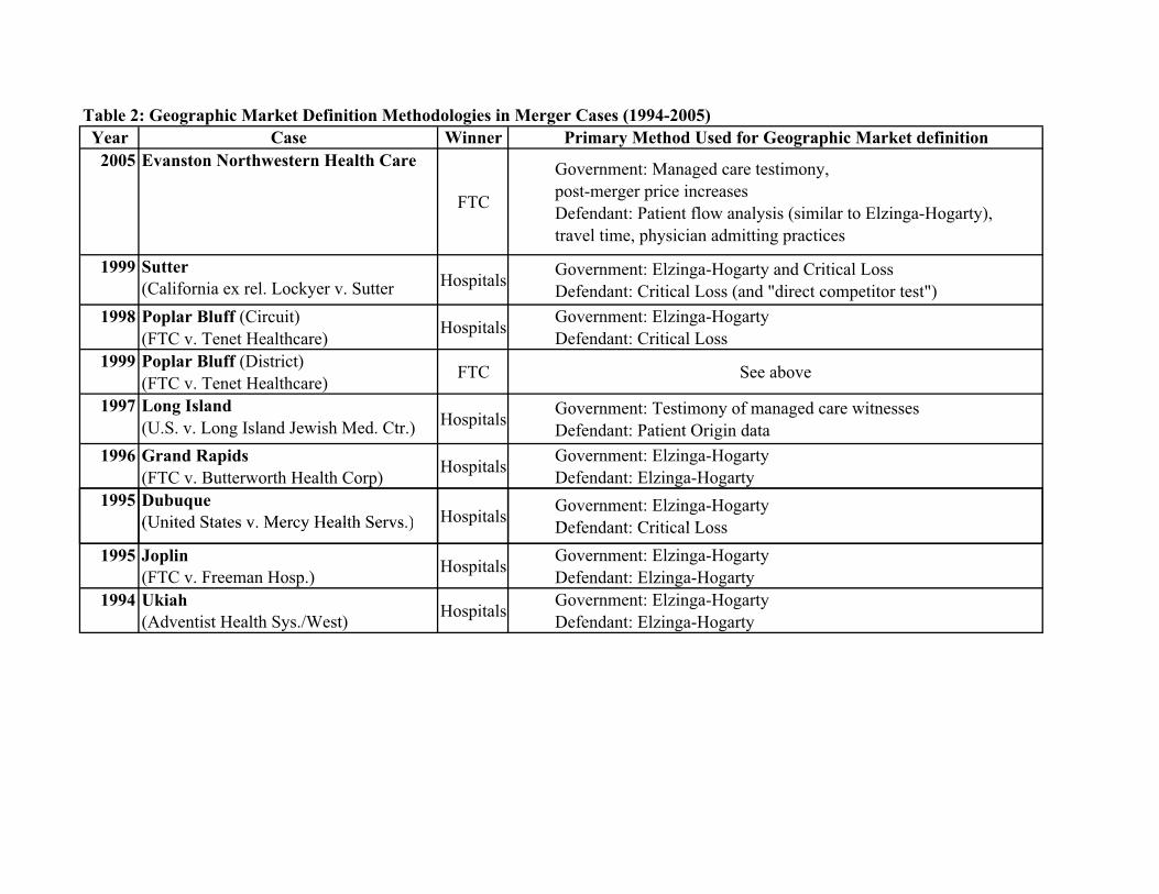
Table 2: Geographic Market Definition Methodologies in Merger Cases (1994-2005)Year Case Winner Primary Method Used for Geographic Market definition

2005 Evanston Northwestern Health Care

FTC

Government: Managed care testimony, post-merger price increases Defendant: Patient flow analysis (similar to Elzinga-Hogarty), travel time, physician admitting practices

1999 Sutter(California ex rel. Lockyer v. Sutter Hospitals Government: Elzinga-Hogarty and Critical Loss

Defendant: Critical Loss (and "direct competitor test")1998 Poplar Bluff (Circuit)

(FTC v. Tenet Healthcare) Hospitals Government: Elzinga-Hogarty Defendant: Critical Loss

1999 Poplar Bluff (District)(FTC v. Tenet Healthcare) FTC See above

1997 Long Island(U.S. v. Long Island Jewish Med. Ctr.) Hospitals Government: Testimony of managed care witnesses

Defendant: Patient Origin data1996 Grand Rapids

(FTC v. Butterworth Health Corp) Hospitals Government: Elzinga-Hogarty Defendant: Elzinga-Hogarty

1995 Dubuque(United States v Mercy Health Servs ) Hospitals Government: Elzinga-Hogarty

Defendant: Critical Loss(United States v. Mercy Health Servs.) osp s Defendant: Critical Loss1995 Joplin

(FTC v. Freeman Hosp.) Hospitals Government: Elzinga-Hogarty Defendant: Elzinga-Hogarty

1994 Ukiah(Adventist Health Sys./West) Hospitals Government: Elzinga-Hogarty

Defendant: Elzinga-Hogarty

Table 3 Summary Data for the Structural ModelConsumer characteristics (N=913,547) MeanQuantity 1.24HMO 0.50PPO 0.31Unscheduled 0.53Distance to chosen hospital 11.60

Hospital Characteristics (N=368)Price 4681% For Profit 28%% Not-For-Profit 52%% Teaching 21%Tech Index 15.10% System Members 50%Beds 192Demand 3070Own-Price Elasticity -4.57Cross-Price Elasticity w/rspt to closest hospital 0.60Cross-Price Elasticity w/rspt to 2nd closest hospital 0.40Cross-Price Elasticity w/rspt to 3rd closest hospital 0.30Cross-Price Elasticity w/rspt to 4th closest hospital 0.21Cross-Price Elasticity w/rspt to 5th closest hospital 0.19

Table 4(N=368)

Critical Loss Elzinga-Hogarty SSNIP Mkt. Def. HSA MSA/PMSA*Number of Hospitals in a Market

Mean 26.75 22.43 3.78 54.38 41.83std. dev 25.63 20.54 2.06 56.18 40.62Median 16 13 3 16 18

Max 89 78 14 130 100Min 2 1 2 1 2

Hospital HHIs (beds)Mean 1505 1460 3874 1031 1005

std. dev 1511 1392 1418 1377 1070Median 875 1026 3683 832 714

Max 6914 10000 8911 10000 5947Min 183 211 1054 118 158

Hospital System HHIs (beds)Mean 1891 1899 3989 1386 1398

std. dev 1716 1577 1442 1500 1260Median 1194 1499 3814 1191 1191

Max 10000 10000 8911 10000 10000Min 356 439 1244 327 366

* The number of MSAs in California is 24. The number of hospitals in the sample that are located in a MSA is 312.

Method of Market Definition

Table 5 (N=93) (N=96) (N=88) (N=91)

Critical Loss Elzinga-Hogarty SSNIP Mkt. Def. Critical Loss Elzinga-Hogarty SSNIP Mkt. Def. Critical Loss Elzinga-Hogarty SSNIP Mkt. Def. Critical Loss Elzinga-Hogarty SSNIP Mkt. Def.Number of Hospitals in a Market

Mean 5.80 7.19 2.78 10.79 9.51 2.80 26.27 23.73 3.64 65.47 50.37 5.96std. dev 5.51 4.69 1.24 9.19 5.55 1.17 11.77 15.30 1.30 13.50 15.18 2.42Median 4 6 2 8 8 2 24 18 4 67 50 5

Max 46 22 10 48 26 7 76 73 7 89 78 14Min 2 1 2 2 1 2 11 7 2 28 9 2

Unique Markets 68 57 73 65 49 73 68 43 72 86 30 79

Difference in Market Size from SSNIP Market Def.Mean 3.01 4.41 - 7.99 6.71 - 22.64 20.09 - 59.52 44.42 -

std. dev 4.98 4.94 - 9.17 5.60 - 11.58 15.15 - 12.96 15.17 -Median 1 3 - 5 5 - 20 16 - 62 44 -

Max 36 20 - 45 23 - 72 68 - 85 73 -Min -3 -3 - -2 -1 - 8 3 - 22 2 -

Hospital System HHIs (beds)Mean 3471 3161 4694 2460 2510 4823 1065 1250 3820 474 592 2552

std. dev 1719 1920 1053 1636 1270 1198 750 683 1441 61 205 675Median 3448 2611 5047 2243 2290 5045 770 1134 3372 468 545 2538

Max 10000 10000 7381 10000 10000 8911 2769 2960 8362 695 1367 5006Min 524 745 1452 392 721 2450 356 439 1814 380 442 1244

Hospitals Operating within Guideline ThresholdsPremerger HHI <1500 8 15 1 24 18 0 72 61 0 91 91 4

1500 � Premerger HHI � 2500 15 30 1 39 40 1 6 24 11 0 0 402500<Premerger HHI 64 48 91 33 38 95 10 3 77 0 0 47

Number of Hospitals within 25 milesMean 2.40 10.71 36.15 93.10

std. dev. 1.61 3.54 16.60 9.93

Quartile 4 (71-110 hospitals)

Market size by quartile of the number of hospitals within a 25-mile radius

Quartile 1(0-5 hospitals)

Quartile 2 (6-18 hospitals)

Quartile 3 (19-70 hospitals)

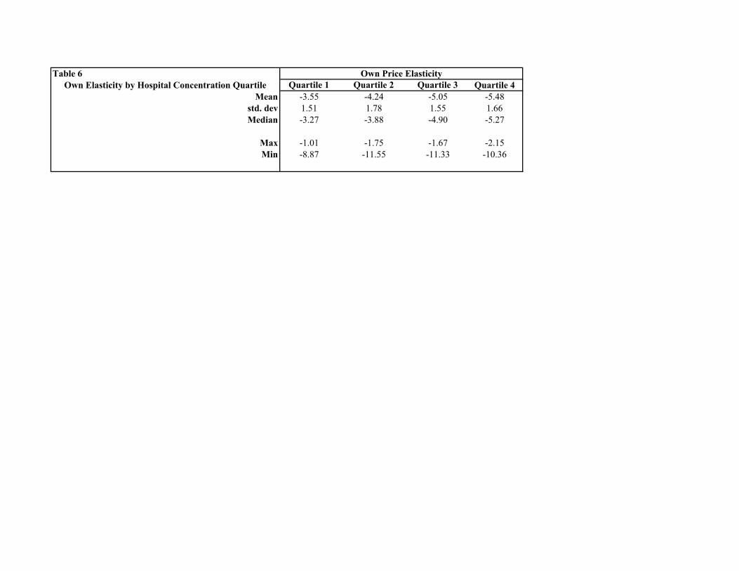
Table 6Own Elasticity by Hospital Concentration Quartile Quartile 1 Quartile 2 Quartile 3 Quartile 4

Mean -3.55 -4.24 -5.05 -5.48std. dev 1.51 1.78 1.55 1.66Median -3.27 -3.88 -4.90 -5.27

Max -1.01 -1.75 -1.67 -2.15Min -8.87 -11.55 -11.33 -10.36

Own Price Elasticity

Table 7 Elasticity by Hospital Density Quartile

Quartile 1 Quartile 2 Quartile 3 Quartile 4Average Estimated Structural Elasticity in Critical Loss Market

Mean -3.60 -4.39 -5.20 -5.48std. dev 0.72 0.89 0.54 0.12Median -3.51 -4.29 -5.39 -5.47

Max -2.17 -2.74 -4.10 -5.09Min -6.35 -8.55 -5.84 -5.84

Average Estimated Structural Elasticity in Elzinga-Hogarty MarketMean -3.89 -4.26 -5.28 -5.41

std. dev 0.91 0.69 0.65 0.14Median -3.72 -4.20 -5.39 -5.43

Max -1.01 -3.22 -4.14 -4.92Min -6.81 -5.99 -6.25 -5.63

Quartile 1 Quartile 2 Quartile 3 Quartile 4Average Implied Structural Elasticity in a Critical Loss Market

Mean -10.10 -13.84 -17.27 -18.65std. dev 7.02 6.86 6.31 3.58Median -8.57 -12.54 -15.36 -18.53

Max -2.27 -2.74 -7.76 -10.51Min -30.35 -48.13 -36.54 -29.02

Average Implied Structural Elasticity in an Elzinga-Hogarty MarketMean -12.55 -13.32 -14.57 -13.10

std. dev 9.41 6.80 8.04 2.37Median -10.15 -10.97 -12.16 -13.60

Max -1.01 -3.23 -6.80 -5.96Min -37.40 -34.81 -32.85 -15.47

Table 8 San Diego HospitalsHospital Ownership Teach Control Tech Index Beds Price Demand Own Price Elasticity # Hosps. Within 25 MilesALVARADO HOSPITAL MEDICAL CENTER Tenet N FP 14 240 3979 2213 -4.48 20SCRIPPS MEMORIAL HOSPITAL - CHULA VISTA Scripps N NFP 8 159 3931 1335 -4.23 17HARBOR VIEW HEALTH PARTNERS Ornda N FP 14 156 3025 1479 -3.50 19THE CORONADO HOSPITAL Sharp N NFP 19 204 4007 562 -4.63 19SHARP CABRILLO HOSPITAL Sharp N NFP 17 227 2535 920 -2.96 19SHARP MEMORIAL HOSPITAL Sharp Y NFP 22 642 4238 15749 -3.92 20SCRIPPS HOSPITAL EAST COUNTY Scripps N NFP 14 162 3440 485 -3.93 19FALLBROOK HOSPITAL DISTRICT N Munic 9 149 4133 665 -3.92 7GROSSMONT HOSPITAL CORPORATION Sharp Y NFP 24 422 3425 9392 -3.29 20MERCY HOSPITAL Scripps Y NFP 16 416 4282 8242 -4.30 19MISSION BAY MEMORIAL HOSPITAL Columbia N FP 18 128 2219 613 -2.66 20PALOMAR POMERADO HEALTH SYSTEM (Escondido) Palomar N Munic 21 389 3874 5247 -3.30 12PARADISE VALLEY HOSPITAL Adventist N NFP 15 228 3035 703 -3.55 18SCRIPPS HEALTH - LA JOLLA Scripps N NFP 27 454 4211 10376 -3.98 21TRI-CITY HOSPITAL DISTRICT N Munic 24 333 2865 5242 -2.10 7UCSD MEDICAL CENTER UC Y NFP 23 359 5827 4193 -5.99 19VILLA VIEW COMMUNITY HOSPITAL N NFP 11 102 5368 26 -6.18 19COMMUNITY HOSPITAL OF CHULA VISTA Sharp N NFP 15 306 4383 2557 -4.15 17PALOMAR POMERADO HEALTH SYSTEM (Poway) Palomar N Munic 20 250 4572 2819 -4.70 19GREEN HOSPITAL OF SCRIPPS CLINIC Scripps Y NFP 24 173 2357 5202 -2.62 21SCRIPPS MEMORIAL HOSPITAL - ENCINITAS Scripps N NFP 16 145 4560 2219 -4.74 18SAN DIEGO HOSPICE CORPORATION N NFP 0 24 3741 55 -4.33 19UCSD LA JOLLA, THORNTON HOSPITAL UC N NFP 13 62 4523 1265 -5.02 21

Table 9Market Definition for San Diego

No. of Hospitals HHI No. of Hospitals HHI No. of Hospitals HHIALVARADO HOSPITAL MEDICAL CENTER 16 2769 14 2960 3 4216SCRIPPS MEMORIAL HOSPITAL - CHULA VISTA 17 2692 18 2228 2 5500HARBOR VIEW HEALTH PARTNERS 16 2696 18 2228 4 3584THE CORONADO HOSPITAL 16 2696 18 2228 2 5089SHARP CABRILLO HOSPITAL 17 2692 19 2454 2 5254SHARP MEMORIAL HOSPITAL 18 2709 19 2454 2 5400SCRIPPS HOSPITAL EAST COUNTY 17 2500 15 2861 2 5991FALLBROOK HOSPITAL DISTRICT 38 775 14 2242 3 4306GROSSMONT HOSPITAL CORPORATION 16 2769 14 2960 2 5378MERCY HOSPITAL 17 2692 18 2228 2 5027MISSION BAY MEMORIAL HOSPITAL 17 2239 19 2454 4 6914PALOMAR POMERADO HEALTH SYSTEM (Escondido) 13 2083 14 2200 3 5496PARADISE VALLEY HOSPITAL 17 2692 18 2228 2 5159SCRIPPS HEALTH - LA JOLLA 16 2464 19 2454 3 8362TRI-CITY HOSPITAL DISTRICT 19 1873 14 2033 2 5773UCSD MEDICAL CENTER 17 2692 18 2228 2 5027VILLA VIEW COMMUNITY HOSPITAL 16 2769 18 2228 4 3029COMMUNITY HOSPITAL OF CHULA VISTA 17 2692 18 2228 2 5500PALOMAR POMERADO HEALTH SYSTEM (Poway) 14 2302 18 2228 3 5143GREEN HOSPITAL OF SCRIPPS CLINIC 16 2464 19 2454 3 8362SCRIPPS MEMORIAL HOSPITAL - ENCINITAS 15 1825 16 2064 3 5003SAN DIEGO HOSPICE CORPORATION 16 2696 18 2228 3 4739UCSD LA JOLLA, THORNTON HOSPITAL 16 2464 19 2454 2 7886

Critical Loss Market Elzinga-Hogarty SSNIP Mkt. Def.

Table 10: Price Increases for Mergers of Independent San Diego Hospitals

Merger (distance between hospitals in parenthesis) Price increase Merger (distance between hospitals in parenthesis) Price increaseMission bay & Alvarado (9.36 miles) Alvarado & Fallbrook (43.09 miles)

Structural Bertrand Model 0.28% Structural Bertrand Model 0.02%WTP Model 0.41% WTP Model 0.03%

Mission bay & Paradise Valley (11.14 miles) Alvarado & Tri-City (31.36 miles)Structural Bertrand Model 0.14% Structural Bertrand Model 0.14%

WTP Model 1.06% WTP Model 0.22%Mission bay & Harborview (6.27 miles) Alvarado & Villa View (2.32 miles)

Structural Bertrand Model 0.39% Structural Bertrand Model 0.04%WTP Model 0.83% WTP Model 0.34%

Alvarado & Paradise Valley (6.4 miles) Alvarado & San Diego Hospice (6.62 miles)Structural Bertrand Model 0.43% Structural Bertrand Model 0.05%

WTP Model 0.48% WTP Model 0.12%Alvarado & Harborview (7.22 miles) Paradise Valley & Fallbrook (48.82 miles)

Structural Bertrand Model 0.61% Structural Bertrand Model 0.00%WTP Model 0.23% WTP Model 0.03%

Paradise Valley & Harborview (5.36 miles) Paradise Valley & Tri-City (36.51 miles)Structural Bertrand Model 0.46% Structural Bertrand Model 0.03%

WTP Model 0.67% WTP Model 0.15%Mission Bay and Fallbrook (39.84 miles) Paradise Valley & Villa View (4.23 miles)

Structural Bertrand Model 0.00% Structural Bertrand Model 0.00%WTP Model 0.24% WTP Model 1.62%

Mission Bay and Tri-City (26.68 miles) Paradise Valley & San Diego Hospice (6.01 miles)Structural Bertrand Model 0.11% Structural Bertrand Model 0.04%

WTP Model 0.75% WTP Model 0.55%Mission Bay and Villa View (8.9 miles) Harborview and Fallbrook (45.58 miles)

Structural Bertrand Model 0.00% Structural Bertrand Model 0.01%WTP Model 1.91% WTP Model 0.03%

Mission Bay and San Diego Hospice (5.24 miles) Harborview and Tri-City (32.70 miles)Structural Bertrand Model 0.01% Structural Bertrand Model 0.08%

WTP Model 1.46% WTP Model 0.14%Fallbrook & Tri-City (13.85 miles) Harborview and Villa View (5.32 miles)

Structural Bertrand Model 1.57% Structural Bertrand Model 0.01%WTP Model 5.30% WTP Model 0.74%

Fallbrook & Villa View (44.85 miles) Harborview and San Diego Hospice (1.25 miles)Structural Bertrand Model 0.00% Structural Bertrand Model 0.05%

WTP Model 0.10% WTP Model 0.30%Villa View & Tri-City (32.71 miles) Tri-City & San Diego Hospice (31.5 miles)

Structural Bertrand Model 0.00% Structural Bertrand Model 0.00%WTP Model 0.11% WTP Model 0.05%

Villa View & San Diego Hospice (5.02 miles)Structural Bertrand Model 0.00%

WTP Model 2.28%

Table 11: Price Increases for Mergers of San Diego Hospital Systems

System Merger Price increaseScripps and Sharp

Structural Bertrand Model 16.11%WTP Model 17.48%

Scripps and UCSDStructural Bertrand Model 3.48%

WTP Model 8.37%Sharp and UCSD

Structural Bertrand Model 3.70%WTP Model 13.31%

Palomar Pomerado and Scripps Structural Bertrand Model 5.40%

WTP Model 8.46%Palomar Pomerado and Tri-City

Structural Bertrand Model 6.18%WTP Model 9.43%

Quartile 1 Quartile 2

Quartile 3 Quartile 4

Figure 1

UCSDMERCY

TRI-CITY

CORONADO

ALVARADOGROSSMONT

FALLBROOK

SD HOSPICE VILLA VIEW

SCRIPPS LJ

SCRIPPS CV

MISSION BAY

HARBOR VIEW

COMM HOSP CV

SCRIPPS EAST

UCSD LA JOLLA

PALOMAR POWAY

GREEN HOSPITAL

SHARP MEMORIAL

SHARP CABRILLO

PARADISE VALLEY

SCRIPPS ENCINITAS

PALOMAR ESCONDIDO

0 7 143.5Miles

LegendHospital Sizebeds

24 - 102103 - 173174 - 306

307 - 454

455 - 642

San Diego Metro Hospitals (N=23)Figure 2

UCSDMERCY

ALVARADO

CORONADO

GROSSMONT

SD HOSPICE VILLA VIEW

MISSION BAY

HARBOR VIEW

SCRIPPS EAST

UCSD LA JOLLA

SHARP MEMORIAL

PARADISE VALLEY

SCRIPPS LA JOLLA

SCRIPPS CHULA VISTACOMM HOSP CHULA VISTA

LegendHospital Size

beds24

25 - 162

163 - 240

241 - 306

307 - 663

Market Defintion for Scripps Chula Vista: SSNIP Market Definition vs Critical Loss

Critical Loss

SSNIP MarketDefinition

UCSDMERCY

CORONADO

ALVARADO

SD HOSPICE VILLA VIEW

MISSION BAY

HARBOR VIEW

UCSD LA JOLLA

PALOMAR POWAY

GREEN HOSPITAL

SHARP MEMORIAL

SHARP CABRILLO

PARADISE VALLEY

SCRIPPS LA JOLLA

SCRIPPS ENCINITAS

PALOMAR ESCONDIDO

SCRIPPS CHULA VISTACOMM HOSP CHULA VISTA

LegendHospital Size

beds24 - 102

103 - 173

174 - 306

307 - 520

521 - 663

Market Defintion for Scripps Chula Vista: SSNIP Market Definition vs Elzinga-Hogarty

Elzinga-Hogarty

SSNIP Market Definition

SHARP CABRILLO

Elzinga-Hogarty:18 hospitalsHHI=2,228

SSNIP Mkt. Def.:2 hospitalsHHI=5,500

SSNIP Mkt. Def.:2 hospitalsHHI=5,500

Critical Loss:17 hospitalsHHI=2,692

Figure 3