A Quantitative, TopologicalModel of Reconnection andFlux Rope Formation in a

Two-Ribbon Flare†

Dana Longcope & Colin Beveridge

Montana State University

I. Sheared Arcade

II. Infinite Arcade

III. Finite Arcade

IV. Energy

V. Rconnection

† Work supported by NSF

1

The 2-ribbon flare

◦ Classical (2d) CSHKP model — (a)

(Carmichael 1964; Sturrock 1968; Hirayama 1974; Kopp and Pneuman 1976)

(b)(a)

A

X

CS XA

RR

S FR

P

C

CC

C

PIL

PIL

◦ 3d generalization (b) — (Gosling 1990; Gosling et al. 1995)

◦ Recon’n flux: magnetic flux swept by flare ribbons (R)

(Forbes & Priest 1984; Poletto & Kopp 1986; Fletcher et al. 2001; Qiu et al. 2002)

◦ Ejected flux rope (FR) → Magnetic Cloud (MC) at 1 AU

(Burlaga et al. 1981; Lepping et al. 1990)

We seek a 3d model quantifying. . .

? Energy storage (vs. shear)

? Reconnected flux (vs. shear)

? Flux in twisted rope (vs. shear)

? Twist in rope (vs. shear)

2

I. The Sheared Arcade

θ

aS/2

a/2

PIL

Photopsheric Flux:◦ Parallel bands of opposing flux

◦ Separated by a◦ Each with Φ′ flux per length◦ Some distribution (profile)within bands◦ May have finite extent L (§III)or L = ∞ (§II)◦ Shear: relative ‖ disp’ment: aS.◦ θ = cot−1S.

◦ 212-D Numerical Simulations (L = ∞)

- Periodic arcades (i.e. periodic boundaries ‖ PIL)

(Mikic et al. 1988, Biskamp & Welter 1989)

- Isolated arcade (Klimchuk et al. 1988, Choe & Lee 1996)

◦ Free magnetic energy: ∆W = W −Wpot

◦ ∆W increases with shearing S — errupts for S ∼> 5

◦ Klimchuk et al. 1988 derive empirical expression:

∆W = Wpot c1 ln(1 + c2S2) , (1)

c1 ' 0.7684 and c2 ' 0.5530

◦ Potential energy depends on profile (through K)

Wpot

L=

K

8π(Φ′)2 , (2)

Gaussian profile: K = 1; Lorentzian profile: K = π/4

3

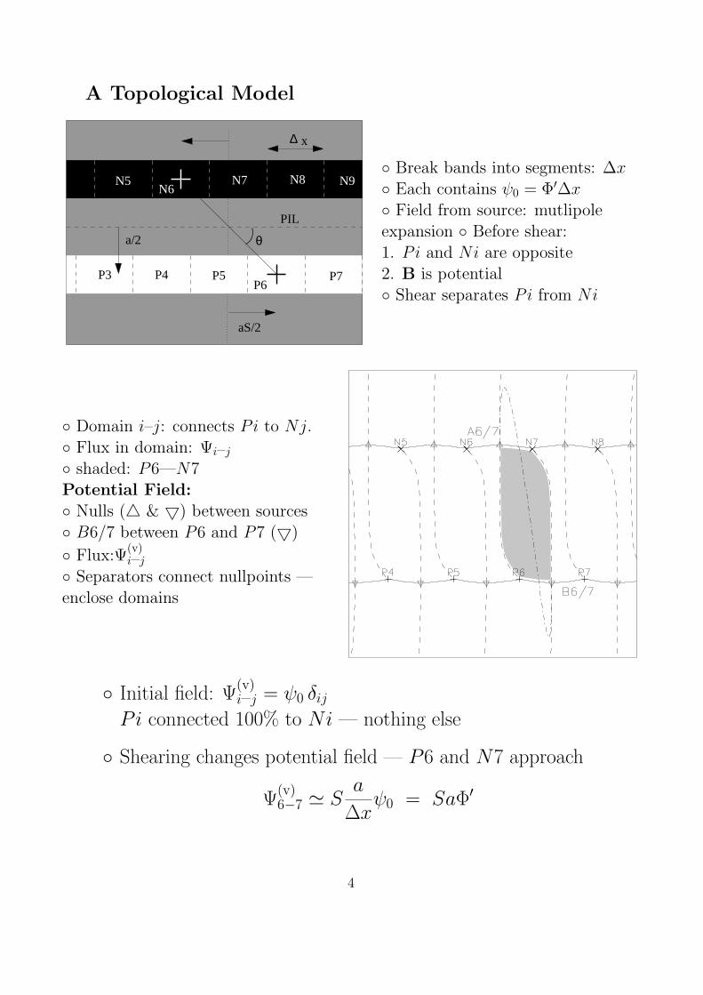
A Topological Model

θ

x

aS/2

N5

P6

N6

a/2

PIL

N9N8N7

P3 P4 P5 P7

∆

◦ Break bands into segments: ∆x◦ Each contains ψ0 = Φ′∆x◦ Field from source: mutlipoleexpansion ◦ Before shear:1. Pi and Ni are opposite2. B is potential◦ Shear separates Pi from Ni

◦ Domain i–j: connects Pi to Nj.◦ Flux in domain: Ψi–j

◦ shaded: P6—N7Potential Field:◦ Nulls (4 & 5) between sources◦ B6/7 between P6 and P7 (5)

◦ Flux:Ψ(v)i–j

◦ Separators connect nullpoints —enclose domains

◦ Initial field: Ψ(v)i–j = ψ0 δij

Pi connected 100% to Ni — nothing else

◦ Shearing changes potential field — P6 and N7 approach

Ψ(v)6−7 ' S

a

∆xψ0 = SaΦ′

4

II. The Infinite Arcade — energy storage

◦ w/o reconnection actual field does not chage: Ψ6−7 = 0

◦ Field cannot be potential: ∆W > 0

◦ Estimate ∆W using MCC (Longcope 1996, Longcope & Magara 2004)

◦ Energy lower bound from FCE — constrain fluxes:

Ψi–j = ψ0 δij

◦ Discrepancy ∆Ψi–j = Ψi–j − Ψ(v)i–j

◦ Leads to current I on separator

I

c` ln(eI?/|I|) + M̃

I

c= − Ψ(v)

expansion about potential field separator properties:

` = length; I? =⊥ shear; M̃ = mutual inductance w/ all others.

Dashed: Equation (1) from Klimchuk et al. (1988)

5

III. The Finite Arcade

◦ L-length bands paritioned into n = L/∆x sources.

◦ 2n− 2 null points between source pairs: e.g. A1/2

L = 4∆x

n = 4

S = 0.1

◦ Large-scale field: dominated by dipole moment (arrow)

6

The Potential Field under increasing shear (L = 4a; n = 4)

S = 0.1

S = 0.3

S = 0.8

7

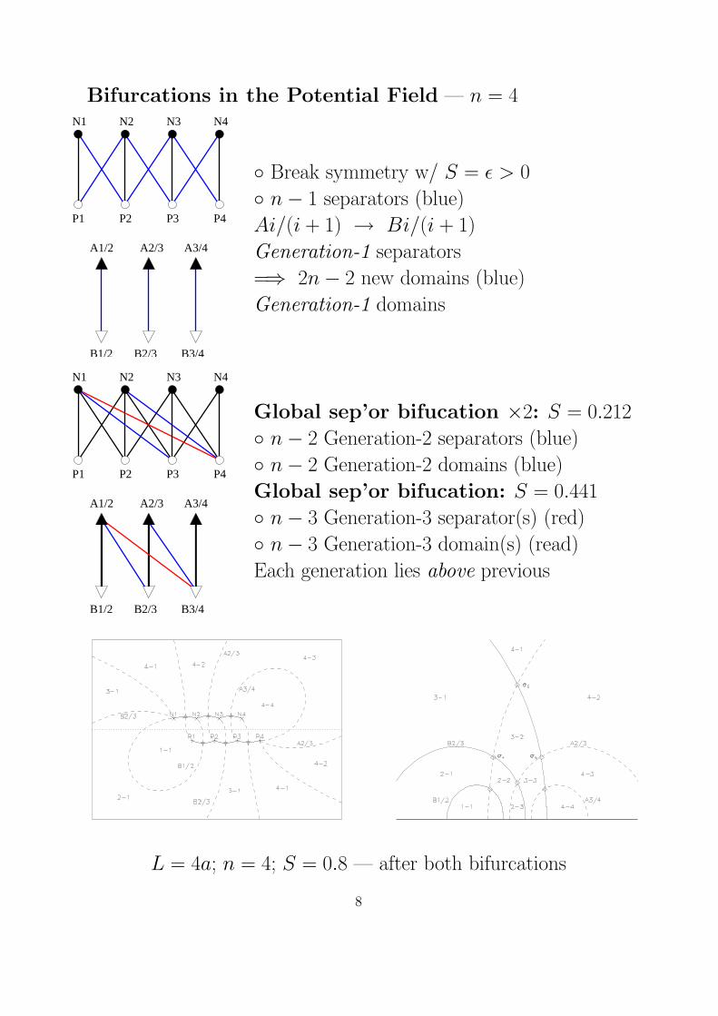
Bifurcations in the Potential Field — n = 4

P1 P2 P3 P4

N2 N3 N4

A1/2

B1/2 B2/3 B3/4

A2/3 A3/4

N1

◦ Break symmetry w/ S = ε > 0

◦ n− 1 separators (blue)

Ai/(i + 1) → Bi/(i + 1)

Generation-1 separators

=⇒ 2n− 2 new domains (blue)

Generation-1 domains

N3 N4

B1/2 B2/3 B3/4

A2/3 A3/4

P1 P2 P3 P4

N1 N2

A1/2

Global sep’or bifucation ×2: S = 0.212

◦ n− 2 Generation-2 separators (blue)

◦ n− 2 Generation-2 domains (blue)

Global sep’or bifucation: S = 0.441

◦ n− 3 Generation-3 separator(s) (red)

◦ n− 3 Generation-3 domain(s) (read)

Each generation lies above previous

L = 4a; n = 4; S = 0.8 — after both bifurcations

8

The Potential Field — general n

L = 4a; n = 8; S = 0.5

◦ Connections made from Pj

N(j+1)NjN(j-2) N(j-1)

Pj

x∆ S a

θ2 θ1PILG0

G1G2R a

◦ Angle θg of connection from generation-g:

cot θg = S +g

n

L

a

9

Bifurcations: — How they depend on S & partitioning (n)

◦ Angle, θg, of bifurcation depends on S, n and generation g.

∃ multiple bifurcations in a generation

◦ =⇒ left edge is creation of field

◦ Limit of continuous field (n→∞) approaches

cot θ ' S +8S√

1 + 4S2

10

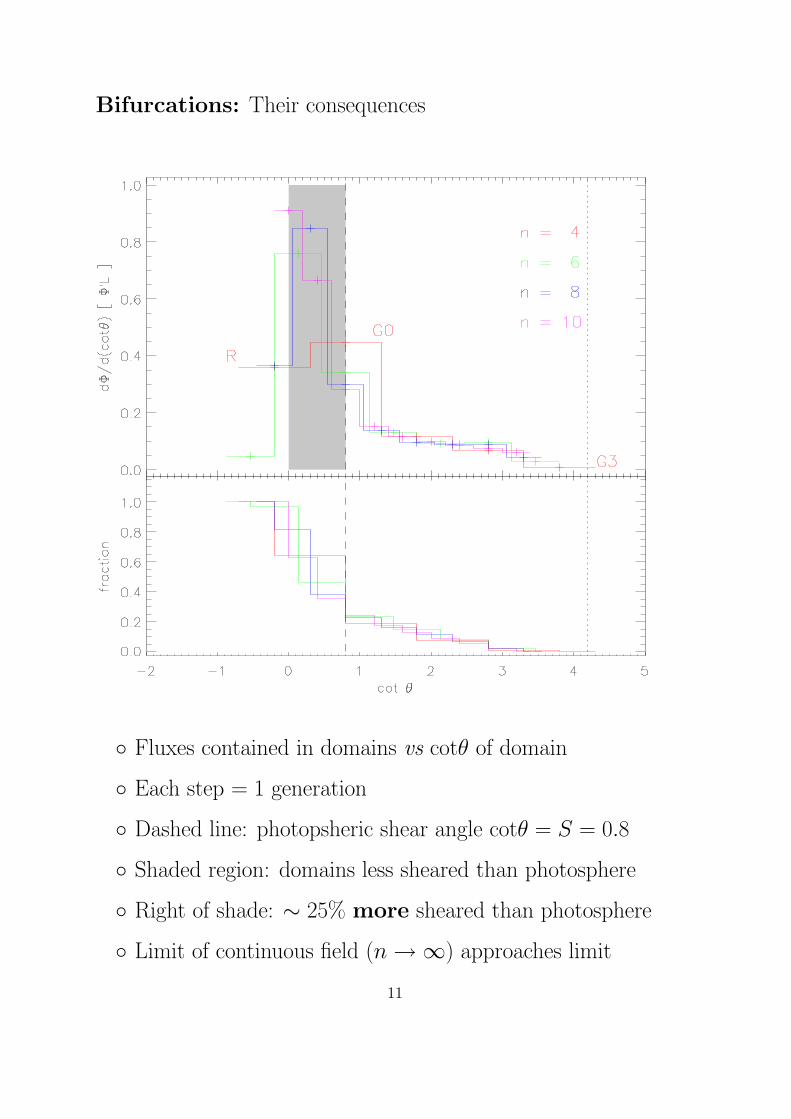
Bifurcations: Their consequences

◦ Fluxes contained in domains vs cotθ of domain

◦ Each step = 1 generation

◦ Dashed line: photopsheric shear angle cotθ = S = 0.8

◦ Shaded region: domains less sheared than photosphere

◦ Right of shade: ∼ 25% more sheared than photosphere

◦ Limit of continuous field (n→∞) approaches limit

11

IV. Energetics

◦ Domain fluxes, e.g. Ψ(v)1–2, Ψ

(v)2–3 . . . increase w/ S

◦ So do fluxes under separators, ψ(v)1 , ψ

(v)2 . . .

◦ Domains retain initial flux: Ψi–j = ψ0 δij

◦ So do separators: ψσ = 0

◦ =⇒ Increasing discrepancies ∆ψσ = ψi − ψ(v)σ = −ψ(v)

σ

12

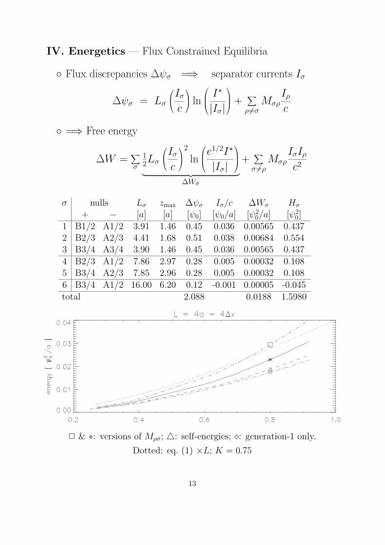
IV. Energetics — Flux Constrained Equilibria

◦ Flux discrepancies ∆ψσ =⇒ separator currents Iσ

∆ψσ = Lσ

Iσc

ln

I?

|Iσ|

+

∑

ρ6=σMσρ

Iρc

◦ =⇒ Free energy

∆W =∑

σ

12Lσ

Iσc

2

ln

e1/2I?

|Iσ|

︸ ︷︷ ︸∆Wσ

+∑

σ 6=ρMσρ

IσIρc2

σ nulls Lσ zmax ∆ψσ Iσ/c ∆Wσ Hσ

+ − [a] [a] [ψ0] [ψ0/a] [ψ20/a] [ψ2

0]

1 B1/2 A1/2 3.91 1.46 0.45 0.036 0.00565 0.4372 B2/3 A2/3 4.41 1.68 0.51 0.038 0.00684 0.5543 B3/4 A3/4 3.90 1.46 0.45 0.036 0.00565 0.437

4 B2/3 A1/2 7.86 2.97 0.28 0.005 0.00032 0.1085 B3/4 A2/3 7.85 2.96 0.28 0.005 0.00032 0.108

6 B3/4 A1/2 16.00 6.20 0.12 -0.001 0.00005 -0.045

total 2.088 0.0188 1.5980

2 & ∗: versions of Mρσ; 4: self-energies; ¦: generation-1 only.

Dotted: eq. (1) ×L; K = 0.75

13

V. Reconnection

Electric field ‖ to separator σ. . .

◦ Will violate constancy of ψσ

◦ Eliminate constraint =⇒ lower possible energy

◦ Breaks pairs of field lines. . . forms new pairs

◦ ψσ changes by passing flux across separator σ

- Remove equal fluxes from two donor domains (red)

e.g. P2–N2 & P3–N3 (from G0)

- Add same flux to two recipient domains (blue)

e.g. P2–N3 (less sheared) & P3–N2 (more sheared)

N3N2

P2 P3

recipient

donor

recipient

donor

0.51

P3-N3

P2-N3

1

P3-N2

1

0.32

0 00.51 0.07

σ2

P2-N2

0.32

◦ Will lower free energy bound

14

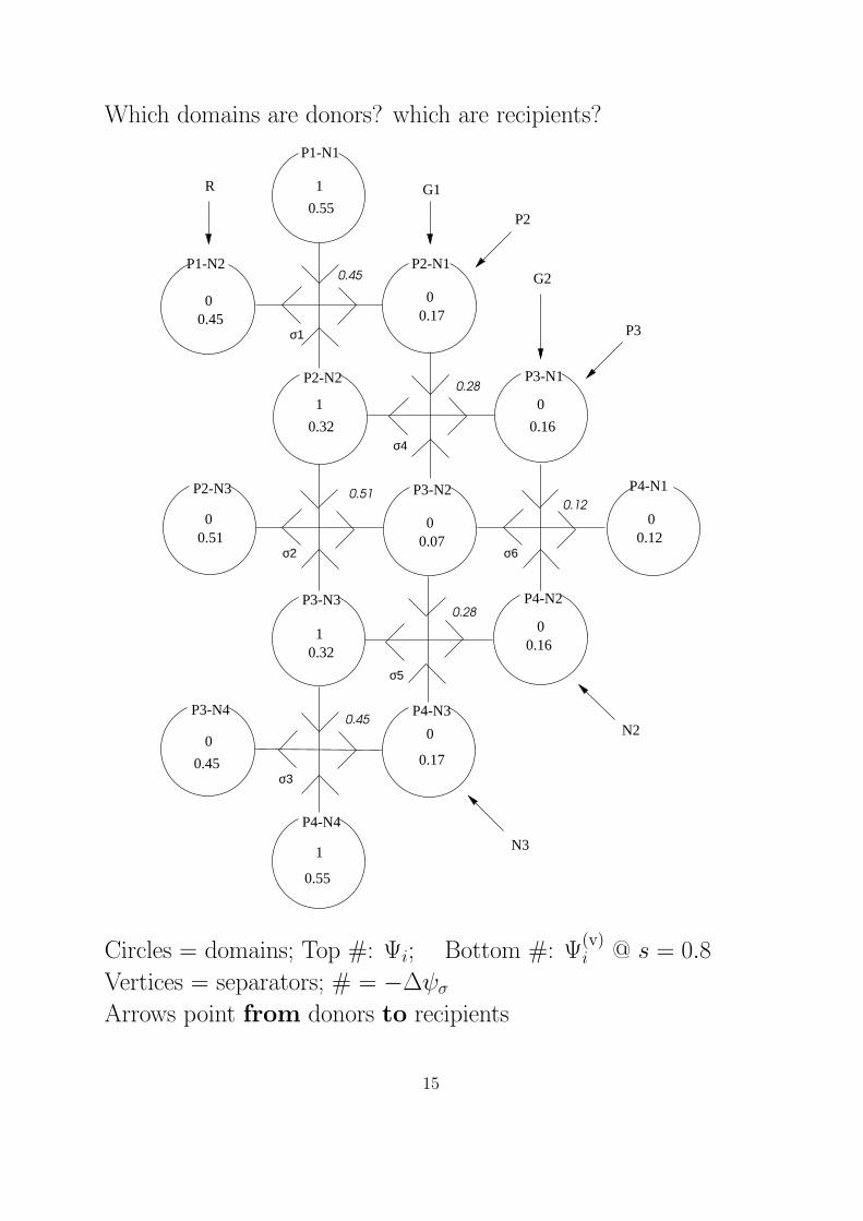
Which domains are donors? which are recipients?

P2

P3

0.51

0.45P3-N4

P3-N3

P4-N4

P2-N2

P4-N2

P4-N3

P4-N1

P3-N1

P3-N2

N3

N2

G2

G1R

0.12

P2-N3

0.28

0.28

0.450

1

0.55

0.45P2-N1P1-N2

P1-N1

1

0

0

0

0

1

0.32

0.170

0

0.16

0.12

0.16

0.070

0

0.170.45

0.51

0.32

0.55

1

σ1

σ2 σ6

σ4

σ3

σ5

Circles = domains; Top #: Ψi; Bottom #: Ψ(v)i @ s = 0.8

Vertices = separators; # = −∆ψσArrows point from donors to recipients

15

First Reconections: Generation-1 separators σ1, σ3, σ3

◦ Fills R (unsheared) domains, P1–N2, P2–N3, P3–N4

◦ . . . and overfills G-1 domains, P2–N1, P3–N2, P4–N3

◦ Remaining constraints =⇒ FCE

σ nulls Lσ zmax ∆ψσ Iσ/c ∆Wσ Hσ

+ − [a] [a] [ψ0] [ψ0/a] [ψ20/a] [ψ2

0]

4 B2/3 A1/2 7.86 2.97 0.28 0.0107 0.00116 0.2345 B3/4 A2/3 7.85 2.96 0.28 0.0107 0.00116 0.234

6 B3/4 A1/2 16.00 6.20 0.12 0.0011 0.00003 0.036

total 0.673 0.0024 0.5031

Second Reconections: Generation-2 separators σ4, σ5

◦ reduces G-1 domains, P2–N1, P3–N2, P4–N3

◦ . . . and overfills G-2 domains P3–N1, P2–N4.

◦ Remaining constraint =⇒σ nulls Lσ zmax ∆ψσ Iσ/c ∆Wσ Hσ

+ − [a] [a] [ψ0] [ψ0/a] [ψ20/a] [ψ2

0]

6 B3/4 A1/2 16.00 6.20 0.12 0.0022 0.00011 0.074

Third Reconection: Generation-3 separator σ6

◦ reduces G-2 domains P3–N1, P2–N4.

◦ fills G-3 domain P4–N1

∆W : 0.018 →︸ ︷︷ ︸first

second︷ ︸︸ ︷0.0024 → 0.00011 →︸ ︷︷ ︸

third0

16

Reconnection: — The consequences

A. Twisted flux rope

◦ Last-generation domain: P4–N1

◦ Above all reconnected flux

◦ ∼ ‖ to PIL

◦ Ψ(v)4–1 = 0.12 — fraction of reconnected flux

◦ Twisted field within domain

- Product of 3 succesive reconnections —

=⇒ 1.5 twists in flux rope (Wright & Berger 1989)

- Self-helicity remaining after mutual helicity is gone

up to Hselfi /2πΨ2

i ∼ 10 turns

- Compare to (cot−1S)/2π = 0.15 turns from shear

17

Reconnection: — The consequences

spines: rims of

reconnected domains

B. Flare ribbons

◦ Total reconnection: ∆ψσ depends on S (approx’ by MCC)

◦ Subsequent generations increase in height

◦ Ribbon motion NOT approximated

Actual reconnection (2d)

MCC reconnection (2d)

18

References

Biskamp, D., & Welter, H. 1989, Solar Phys., 120, 49Burlaga, L., Sittler, E., Mariani, F., & Schwenn, R. 1981, JGR, 86, 6673Carmichael, H. 1964, in AAS-NASA Symposium on the Physics of Solar Flares, ed. W. N. Hess

(Washington, DC: NASA), 451Choe, G. S., & Lee, L. C. 1996, ApJ, 472, 360Fletcher, L., Metcalf, T. R., Alexander, D., Brown, D. S., & Ryder, L. A. 2001, ApJ, 554, 451Forbes, T. G., & Priest, E. R. 1984, in Solar Terrestrial Physics: Present and Future, ed.

D. Butler & K. Papadopoulos (NASA), 35Gosling, J. T. 1990, in Geophys. Monographs, Vol. 58, Physics of Magnetic Flux Ropes, ed.

C. T. Russel, E. R. Priest, & L. C. Lee (AGU), 343Gosling, J. T., Birn, J., & Hesse, M. 1995, GRL, 22, 869Hirayama, T. 1974, Solar Phys., 34, 323Klimchuk, J. A., Sturrock, P. A., & Yang, W.-H. 1988, ApJ, 335, 456Kopp, R. A., & Pneuman, G. W. 1976, Solar Phys., 50, 85Lepping, R. P., Burlaga, L. F., & Jones, J. A. 1990, JGR, 95, 11957Longcope, D. W. 1996, Solar Phys., 169, 91Longcope, D. W., & Magara, T. 2004, ApJ, 608, 1106Mikic, Z., Barnes, D. C., & Schnack, D. D. 1988, ApJ, 328, 830Poletto, G., & Kopp, R. A. 1986, in The Lower Atmospheres of Solar Flares, ed. D. F. Neidig

(National Solar Observatory), 453Qiu, J., Lee, J., Gary, D. E., & Wang, H. 2002, ApJ, 565, 1335Sturrock, P. A. 1968, in IAU Symp. 35: Structure and Development of Solar Active Regions,

471Wright, A. N., & Berger, M. A. 1989, JGR, 94, 1295

19