A PRIORI ESTIMATION OF VARIANCE FOR

SURVEYING OBSERVABLES

B. G. NICKERSON

November 1978

TECHNICAL REPORT NO. 217

TECHNICAL REPORT NO. 57

PREFACE

In order to make our extensive series of technical reports more readily available, we have scanned the old master copies and produced electronic versions in Portable Document Format. The quality of the images varies depending on the quality of the originals. The images have not been converted to searchable text.

A PRIORI ESTIMATION OF VARIANCE FOR SURVEYING OI~SERV ABLES

B.G. Nickerson

Department of Geodesy and Geomatics Engineering University of New Brunswick

P.O. Box 4400 Fredericton, N .B.

Canada E3B 5A3

November 1978 Latest Reprinting January 1998

ACKNOWLEDGEMENTS

This work was partially funded by contract no. 132 730 from the

Land Registration and Information Service to the University of New

Brunswick. The help provided by Dr. D.B. Thomson during the writing of

this report was particularly invaluable. The comments supplied by Dr.

A. Chrzanowski are also appreciated. Ms. S. Biggar is acknowledged for

her excellent typing.

TABLE OF CONTENTS

1. INTRODUC'l'ION • • • •

2. ANGULAR MEASUREMENTS

2.1 Internal .••••..•....

2.1.1 Pointing Error ..•...• 2.1.2 Reading Error ..•.... 2.1.3 Leveling Error ..•••.• 2.1.4 Summary of Internal Accuracy

2.2 External .•.

2.2.1 Zenith angles . . . . . . . . . . . . . 2.2.1.1 2.2.1.2 2.2.1.3 2.2.1.4

Empirically Determined Refraction Angle •• Simultaneo~s Reciprocal Zenith Angles •... Analytically Determined RefractL:::n • Height of Target

2.2.2 Horizontal Angles· · ·

2.3 Other Error Sources Encountered for Azimuths

2. 3. 1 Gyro Azimuths . . • • . • . • . • . • • 2.3.2 Azimuths Determined from Star ~bersvations

2.4 Summary ••.•

2.4.1 2.4.2 2.4.3 2.4.4 2.4.5 2.4.6

Directions Horizontal Angles • Zenith Angles ... Astronomic Azimuths • Geodetic Azimuths • "Grid" Azimuths

3. DISTANCE HEASUREMENTS . . •

3.1 EDM

3.lol Internal • 3.1.2 External • 3o1.3 Summary of Variance for EDM

3.2 Mechanical Distance Measurement ..

3o 3 Optical Ci..stance Measurement • • • . . o

3.3.1 Stadia Tacheometry 3.3.2 Subtense Bar o •.••

l

3

3

3 5 6 8

11

ll

12 14 15 16

16

19

19 21

25

25 26 28 29 29 30

30

30

31 35 41

42

44

44 46

3. 4 Summary • o • • • • o • . • • . . • o . . . • • . • • • 48

LIST OF FIGURES

Figure 2.1 Zenith Angle Measurement

Figure 2.2 Reciprocal Zenith Angles

Figure 2.3 Effect of Lateral Ref£action

Figure 2.4 Angles and Directions •

Figure 3.1 Reduction of Distances

Figure 3.2 Tape in Catenary . . .

Figure 3.3 Stadia Measurements . • . •.

Figure 3.4 Bar at End

Figure 3.5 Bar in the Middle

Figure 3.6 Auxiliary Base at End

Figure 3.7 Auxiliary Base in the Middle of the Line

11

14

17

27

38

43

45

46

47

47

48

:Figure 3. 8 Expected Relative Precision of Subtense Bar r1easurements • 49

LIST OF TABLES

Table 2.1 Major Features of Some Modern Theodolites . . . . . . . . . . 4

Table 2.2 Internal Accuracy Default Values . 9

Table 2.3 Expected Centering Error . . . 18

Table 3.1 EDM Instruments . . . . . '. . . . . . . . . . . . . . . . 32

Table 3.2 Effect of Heteorological Errors on Measured Distances . . . . 37

: i i

1. INTRODUCTION

Observational~accuracy in contemporary surveying practice is

characterized by the standard derivation or variance of individual obser­

vations. In order that useful statistical propagation of this error

can occur, these variances are assumed to have a normal,distribution with

zero mean. This implies that the variances must be composed of random

errors, and that any error or inaccuracy which is systematic in nature has

already been accounted for and removed, either by solving for the systematic

component through an adjustment process, eliminating it through appropriate

observation procedures, or eliminating it by other empirical techniques.

This report is intended to provide an analysis of the random

errors inherent in observations encountered in surveying, which are

used to estimate the variances of these observations. It must be made

clear from the outset that the systematic errors encountered in surveying·

measurements are not considered directly. They are, however, given the

attention necessary to evaluate the effect of errors made in eliminating

or minimizing these systematic biases. This is necessary to compute

realistic variances for the indi~ldual observations.

With this in mind, the errors are split into 2 distinct sections.

The first covers random errors encountered when making angular ~easurements.

The accuracy of directions, vertical and horizontal angles, and azimuths

are all examined, although, as one would expect, they are very much

interrelated. The second sect~on deals with the random errors encountered

when measuring distances. The accuracy of various electromagnetic distance

measuring (EDM) equipment as well mechanical (e.g. chain) and optical

methods are treated.

1

2

Only these basic surveying observables are analysed, and

obs·~rvations such as inertial, Doppler or hydrographic (e.g. range-range)

measurements are not covered.

3

2. ANGULAR MEASUREMENTS

The term angular accuracy, in this report, refers to the

accuracy of making measurements with a modern theodolite such as a Wild T2

or Kern DKM2. Various types of theodolites are available, and Tabl,e 2, [Cooper

1971) gives an excellent summary of the major features of some of

the theodolites in use today.

This work does not intend to describe or assess the mechanical

or optical components of theodolites. It is assumed that either the

theodolite is in correct adjustment, or that ~ny misalignment or other error

can be eliminated by suitable observation procedures (e.g. mean of face

left and face right readings corrects for line of collimation

not being perpendicular to the axis of the theodolite). For those who

are interested in theodolite construction, and its detailed analysis, an

excellent reference is Cooper [1971]. Instead, tr.e topics dealt with are

concerned with random errors which arP unavoidable in the everyday use of

theodolites, and with obtaining reasonable estimates for them.

2.1 Internal

Internal errors are those which are caused by the actual equipment

and/or observer using it. Errors considered under this heading include

pointing, reading and levelling errors.

2.1.1 Pointing Error

The pointing error a is di:!:ectly related to the telescope magnification p

of the individual theodolite. Chrzanowski [1977] states that the maximum

accuracy of pointing is 10"/H, where M is the telescope magnification. He

I Telescope I H. Circle I If. Circle I Readinq

MANUFACTURER! COUNTRY

I Magni- 1 Objective llen~th I Shortest I Fle1d of I Oiam.l Gradu-~ Diam., Gradu~1 Direct I System fication, dlam(rrm) (mm) Focus (m) View (•) (r.m) ation (lllll) ation , to

FTJA 01(!'-1 Kl-A Te-E6 Microptic 1 4149-A V22 Tl6 TIA Theo 020 Th 3 1h 4 Tu H2 OK!-' 2 OYJ~ 2-A TS ·1

I Fennel I W. Germany Kern Switzerland Kern Switzerland

30 20 28

~1om i Hungary 20 Rank U.K. 25 Sa 1mi rag hi Ita 1y 30 Vickers U.K. 25 Wild Switzerland 28 Wild Switzerland 28 Ziess~Jena) E. Germany 1 25 Zeiss Ober.) W. Germany I 25 Zeiss Ober.) W. Germany 25 Askanla W. Germany 30 Fenne 1 W. Germany 30 Kern S\"litzerland I 30

j Kern I S1vitzerland 30 , :iash- USSR 26 I priboritorg j I

Te-B3 ~1· l'.om Hungary 30 i'icroptic 2 ?ank 'I U.K. I 28 '200-A 1 SJlmoiraghi Italy I 30 Tavlstock ~Vickers U.K. I 25 T2 1 ~'i 1 d I S1vitzerl and 28 T~eo 010 'Zeiss(Jena) E. Germany 131 Th2 !Zeiss (Ober.)lw. Germany 30 >~'3 :Kern j' Switzerland 27,45 "T-02 I ~·~sh- USSR 24,30,

priboritorq I 40 "icro!ltic 3 PMk 1 U.K. 40 ~end. Tavi. Vickers jU.K. 20,30 T3 II Wild 1 Switzerland 24,30

I 40 T4 Wild Switzerland 70

I I I

40 30 45 28 38 35 38 40 40 35 35 35 45 45 as 45 40

40 41 40 on vO

40 53 40 72 60

50 60 60

60

I 175 I 120 I 155

123 146 172 137 150 150 195 150 150 165 174 170 170 180

175 165 172 159 150 135 155 140 265

i 70 225 265

1.2 0.9 1.8 1.3 1.6 2.0 1.8 1.4 1.4 2.1

.1.2 1.2 1.5 2.0 1.7 1.7 1.2

2.5 1.8 2.5 1.8 1.5 2.0 1.6 19 5.0

1.8 5.0 3.6

100

1.6 1.7 1.5 2.0 1.5 1.4 2.0 1.6 1.6 1.6 1.7 1.7 1.6 1.6 1.3 1.3 1.3

1.5 1.5 1.5 2.0 1.6 1.2 1.3 1.6 1.6

1.0 1.3 1.6

90 50 89 80 89 90 78 79 73 96 78 98 90 93. 75 75 85

II 78 98

I 40 85 90 84

100 100 135

98 127 135

240

j•

20' j•

20' 20' 30" ]0

1" 1" j•

1" 1" 20' 20' 10' 10' 20'

20' 10' 10 1

20' 20' 20 1

10' JO' 4'

5' 20' 41

21

70 50 70 40 64 90 63 79 65 i4 70 85 70 60 70 70 75

66 76

., ~~ 70 60 85

100 90

76 70 90

135

1 0

20' 1" 20' 20' 30" j•

1" 1" 1" 1" 1" 20' 20 1

10' 1 0' 20'

20 1

10 1

10' 20 1

20 1

20 1

10' 101 8'

5' 20' 8'

4'

i I

10" 20" 10" 20" 30" 20" 1 I 20" j I

30" 1 • 1" 1" 1" 1" 1"

Opt. Scale Opt. micro Opt. micro Opt. micro Opt. micro Direct Opt. scale Opt. scale Opt. micro Opt. scale Opt. micro Opt. scale Coinc. micro Coinc. micro Co!nc. micro Coi nc. micro Caine. micro

1" Coinc. micro 1" Coinc. micro 1" Coinc. micro 1" Coinc. micro 1" Coinc. micro 1" Coinc. micro 1" I Caine. micro

0~5 Coinc. micro 0~2 Coinc. micro

0~2 I Coinc. micro o:·s&l" I Caine. micro

0~2 I Coinc. micro

~0~1/0~2 Coinc. micro

I

Table 2.1 Hajor Features of Some Modern Theodolites

Sp1rit levels Value of 2 r.ml Plate I Altitude

( •) i")

40 30 40 50 40 30 45 30 30 30 30 30 20 20 20 20 20

20 20 20 20 20 20 20 10 7

10 20 7

auto. 30

auto. auto.

30 auto. 90 30

auto. auto. auto. auto. auto.

20 20

auto.

1- a::o.

20 auto.

20 30 20

auto. 10

I :: 10 30

2

i

I

I

Spherical jweight (') I {kg}

8

6

10 17 8 8 8

15 10 10 6

12

6

10 20 8 8

10

8

l I 4.0

1.8 ' 4.2 1 2.6 I 4.5 1 4. 7 I 5.2

4.5 1 s.o : 4.3 I 3.5 l 4. 5 ! 4.6 ' 5.5 : 3.6

6.8 5. 1

5.5 6.3 6.1 4.8 5.6 5.3 5.2

12.2 11.0

8.0 i 9.8

11.2

I 60

-~

I I ! l

""

5

further states that this minimum error is increased by improper target

design, imperfect atmospheric conditions and focussing error. In average

visibility and thermal turbulanc.,; conditions with a well designed target,

one can expect a pointing error of

30" cr =

p 11 up to cr

p 60"

~1 ( 2-1)

for a single pointing at distances larger than a few hundred meters.

Roelofs [1950] is in substantial agreement as he concludes that the accuracy

of pointing on a star is IJ, = 70" /M for either the horizontal or vertical p

crosshair. This seems ~easonable considering that pointing on a moving

star is not as accurate as pointing on a stationary target.

One can expect, then, to obtain the above error due to pointing

in average conditions. The pointing error is partially due to personal

error, and procedures outlined in section 2.1.4 el:able one to determine

the pointing errcr as well as the other internal errors discussed here.

One can expect the pointing error to be larger when poor visibility or

large thermal turbulence (e.g. scintillation) occur.

2.1.2 Reading Error

Reading error cr is prir:tarily a function of the least count or r

smallest angular division of the theodolite. Error is also introduced

if there are graduation errors in either the horizontal circle or the

micrometer scale (for those theodolites which have micrometers). These

graduation errors are assumed to be negligible due to observation

procedures designed to

6

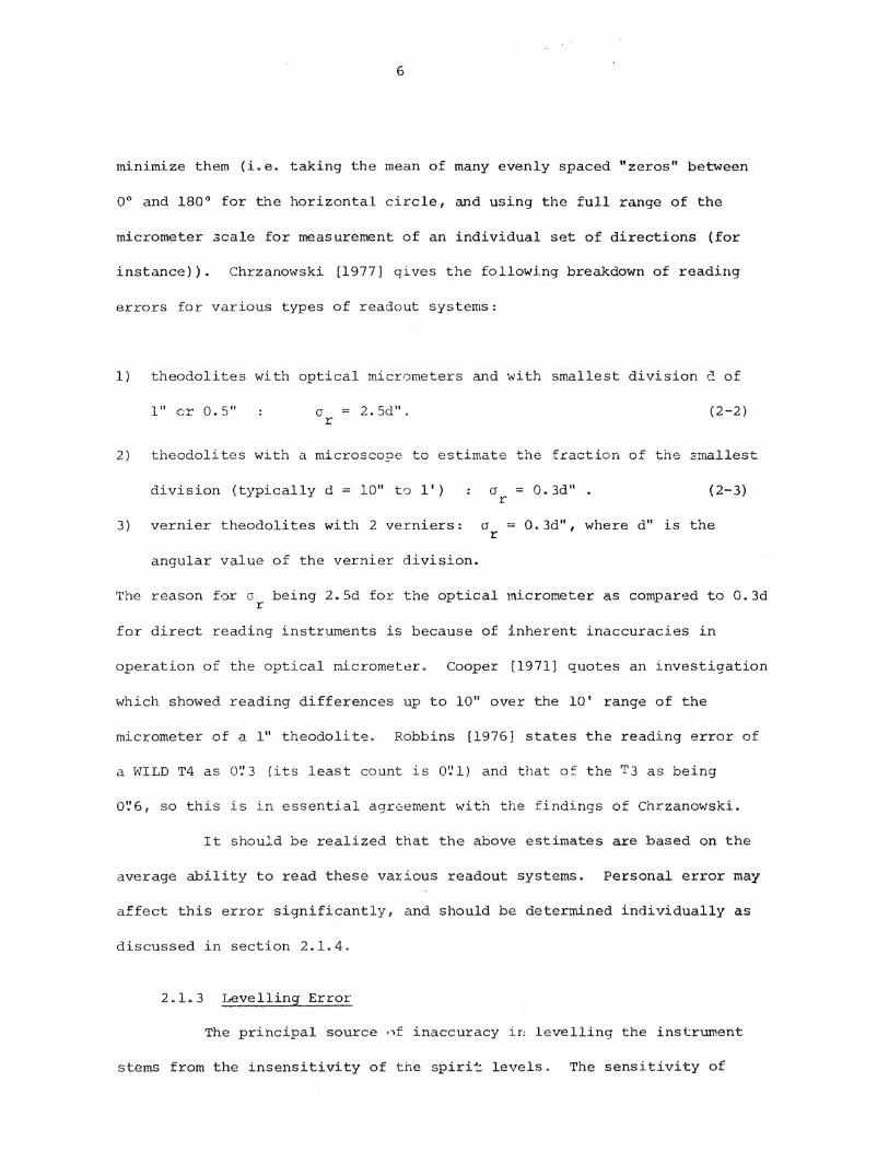
minimize them (i.e. taking the mean of many evenly sp~ced "zeros" between

0° and 180° for the horizontal circle, and using the full range of the

micrometer 3cale for measurement of an individual set of directions {for

instance)). Chrzanowski [1977] gives the following breakdown of reading

errors for various types of readout systems:

1) theodolites with optical micrometers and with smallest division c of

1" cr 0.5" a = 2. Sd". r

(2-2)

2) theodolites with a microscope to estimate the fraction of the smallest

3)

division (typically d = 10" to 1') (J = 0.3d" r

(2-3}

vernier theodolites with 2 verniers: a = 0.3d", where d" is the r

angular value of the vernier division.

The reason for o being 2.5d for the optical 1\'\icrometer as compared to 0.3d r

for direct reading instruments is because of inherent inaccuracies in

operation of the optical micromet~r. Cooper [1971] quotes an investigation

which showed reading differences up to 10" over the 10' range of the

micrometer of a 1" theodolite. Robbins {1976] states the reading error of

a WILD T4 as 0~3 (its least count is 0~1) and that of the T3 as being

0~6, so this is in essential agr6ement with the findings of Chrzanowski.

It should be realized that the above estimates are based on the

average ability to read these various readout systems. Personal error may

affect this error significantly, and should be determined individually as

discussed in section 2.1.4.

2.1.3 Levelling Error

The principal source •."lf inaccuracy in levelling the instrument

stems from the insensitivity of the spirit levels. The sensitivity of

7

spirit levels is characterized by their bubble value, which is the angular

value.necessary to displace the bubble through 1 of the divisions marked

on the top of the spirit level. 'J'hese divisions are usually placed 2

mm apart [Cooper, .1971]. Both Chrzanowski [1977] and Cooper [1971] state

that it is possible to center the bubble to an accuracy or. about 1/5

of one division. Thus, for a bubble value v", the accuracy that can be

expected for levelling the spirit level is

ov = 0.2 v" . (2-4)

This value is, of course, only valid for good conditions (i.e. one side of

thetheodolite not heated more than the other side, stable tripod, spirit

level correctly adjusted, etc.). The bubble values of various theodolites

are listed in Table 2.1.

A spirit level which is centered by a coincidence reading

system (i.e. split bubble) is, according to Coo~er (1971], able to be

centered ten times as accurately as by viewing the bubble directly. Thus,

a split bubble centering system, which is used by many manufacturers

on the vertical circle bubble, has

0 v

0. 02 v".

a levelling accuracy of

(2-5)

Hany present day theodolites have automatic compensators for the

vertical circle. Cooper [1971] states that most 20" instruments claim an

accuracy o = 1~0 and that the Kern DKM2-A has o = 0~3. One method of v v

determining the accuracy of compensation is to take various readings of

the vertical angle on a fixed target, each time moving one of the footscrews

i.n order to take the compensator through its full working range. After

removing the effects of reading and pointing errors, the resulting spread

of readings will be due to the automatic compensation.

8

The. above discussion of the error in levelling has been

concerned with the accuracy levelling the instrument itself. What is

of real concern is how this inaccuracy affects the actual angular accuracy

of one pointing of the theodolite. Cooper [1971] and Chrzanowski [1977]

both concur that the levelling inaccuracy has an eff~ct of

a " = a " cot h L v

(2-6)

on a measured direction, where

h = zenith angle to target.

Thus, for small vertical angles, crL is negligible, but for steep lines

of sight, aL is an increasing source of error.

2.1. 4 Summar~ Internal Accuracy

In concluding this section, the internal accuracy is given as

2 a. ~

= a 2

p + a r

2 2 + a

L (2-7)

for one pointing of the telescope, and this figure ~s dependent on the

instrument being used as well as the personal Liases of the individual

user.

The rr.ethod used in the North American Readjustment [Pfeifer, 1975)

as well as in the Maritime Provinces Second Order Readjustment [Chamberlain,

1977) is to compute the internal error for each mean direction in the sets

9

of directions at each station by means of a station adjustment [Mepham,

1976]. This analytical method qives a good estimate of the internal

accuracy achieved for each individual direction, but is still composed

of the 3 elements discussed above. Some default values of internal accuracy

for typical types of surveys are given by Pfeifer [1975], and are listed

here in table 2.2.

Order of Class of Nominal Relative Internal Accuracy Survey Survey Accuracy a.

~

l 1:100 000 0~33

2 l 1:50 000 0~33

2 2 1:20 000 0~47

3 l 1:10 000 0~69

3 2 1:5 000 1~39

Table 2.2 Internal Accuracy Defawlt Values

The final part of this section will describe a method which

enables one to compute the expected reading, pointing and levelling errors

for a particular the~dolite and observer. The procedure is essentially

the same as that carried out in a lab for course SE 3022.taught by

Dr. Chrzanowski at the University of New Brunswick. The initial steps are

to set up the instrument and tripod in normal conditions (e.g. outside on

a cool day on a grassy slope) and center it over some point. The following

steps then enable one to determine the reading, pointing and levelling

accuracy:

10

1) Take 20 different readings of the same pointing. All that this

involves is the setting of the coincidence of the vernier or micro-

meter hairs, and reaqing the setting 20 s~parate times. By taking the

mean of the 20 readings and computing the standard deviation, one

arrives at the reading error a ~ r

2) Take 20 different pointings and readings combined. This involves

pointing the cross hairs on a stationary target, making a reading,

moving the cross hairs off the target, pointinq and reading again,

etc. The s~andard deviation of these will give the combined pointing

and reading error ~ 2 + cr 2 and by the law of propagation of errors, the r P

pointing error is computed as

2 a

p = (a 2 + a 2)

r P 2

- a r

(2-8)

3) The same pointingsand readings are made as in step 2, except that now

the instrument is thrown off level between each pointing and reading,

and relevelled before each one. As already mentioned, this error

should be negli~ible for small vertical angles, and the instrument

in correct adjustment, but it would serve to estimate the levelling

error if one was expecting to measure steep lines of sight. This

standard deviation of these readings will yield the combined reading,

pointing and levelling error, and aL is co~puted as

2 2 2 = (a + a + aL )

r P (0 2

r (2-9)

4) The centering error, which is discussed in section 2.2, can also be

determined in this procedure. The same steps as carried out in step 3)

are performed for each reading, except that now, the instrument and

11

tribrach together are turned through 120° and recentered between each

reading. This set of readings will yield the combined centering,

reading, pointing and levelling error, and by subtracting the variance

obtained from 3} from the variance of the readings of 4}, the accuracy

of centering can be determined.

2.2 External

External inaccuracies stem from uncertainties in the determination

of environmental factors such as refraction. As well, inaccuracies which

are proportional to the distance between stations, although not strictly envi­

ro~~entally dependent, are included here. As can be expected, zenith

angles are affected differently by the environment than are horizontal

angles; thus, this section is divided into these two categories.

2.2.1 Zenith Angles

The primary cause of random error in zenith angles is the

inaccuracy in determination of the vertical refraction. As indicated in

Figure 2.1, refraction causes the ray of light between two stations to be

curved, thus causing the desired zenith angle z to be in error

direction of vertical E = measured zenith angle

refraction angle

- required zenith angle

= height of instrument

= height of target

Figure 2.1 .Zenith Angle Measurement

12

by e:. The random error in the zenith angle z is

0 z 2 2

+ 0 (2-10)

assuming no correlation between E and E:. The inaccuracies involved in

determining E have already been discussed in the pn:!vious section, so

the problem remains to determine a_ 2• This will depend on the method used t.

to determine or eliminate the refraction angle s. The 3 basic methods

presently used to handle vertical refraction are

l) Add the empirically determined refraction angle to the observed zenith

angle E.

2) Measure simultaneous reciproc:1l zenith angles to eliminat.e the effect

of the refracti~n angle.

3) ~1odel the vertical refractL..,n into an adjustment includinc:r neasured

zenith angles to determine ' analytically.

2.2.1.1 Empirically Determined ~efraction Angle

If the vertical or zenith angle is measured from only one end of

the observing line, the refraction angle must be determined by empirical

methods. This is usually accomplished by use of the ;oefficient of refraction

k in the relationship (e.g. Faic:r, 1972]

where k

E: = ks 2R

coefficient cf refraction,

s = distance between the 2 stations,

( 2-11)

R = mean radius of curvature of the earth between the· 2 ·stations.

The primary inaccuracy in (2-11) stems from inadequate knowledge of k,

and thus

13

(2-12)

The coefficient of refraction can ,be computed as [Angus-Leppan, 1971]

where P

aT ah

T

k ()'I'

(0.0341 + {lh ) ,

air pressure in millibars,

tempe~:ature in degreElS Kelvin,

temperature gradient ~Ln degrees Celcius per meter.

(2-13)

'I'he tempera·ture gradient in (2-13) is the most difficult item to ascertain.

Angus-I..eppan (1971.] quotes valtE:S of -4°C/m for hEdght.s of l em to 1 m

above ground, -0.8" Cjm from one metre to 2 met;:es above t.he surface, and

····0. 03" :=;rn from 2 to 100 m above ,Jround for the temperature orad.ient

a function of many things including dens.i ty o:: the air, temperature, soil

characterist.ics under the sight line, wind speed, etc. (see A:.i.gus···Leppan

[1971]), but when observing lines are high above the ground at mid-day

or afternoo:J., t.he values of {l'r/ ?h approaches -0.0055, which corresponds

t.o a value for k cf 0.13. Invest:Lgat.ions carried out by Angus-It::ppan

[1961] to determine~ an empirical formula for E by measuring temperature

gradients along lines of sight close to the ground (i.e. 5 feet to 30 feet)

resulted in an accuracy of no better ·than cr ""' 5" for a sight line 3600 E:

feet long, which is an accuracy of about 4~5/km. It is apparent that the

empirical. met.hod of det.ermination of k is not accurat.e (using pre.sen·t

inst.rumentat:ion) even in the best. of situations. Work is presently being

carried out [Bamford, 1975] to det:ermine the refraction directly by

mec-,suring the dispf;rsi.on of two differf.mt coloured lig·ht. beams, but it. is

still in the development stages.

14

2. 2. L 2 Simultaneous Reciprocal Zenith Angles

This method of accounting for refraction is depicted in Figure

2. 2.

Figure 2. 2 Reciprocal Zenith £\ngle";

'l'he basic assumption is that the refraction angle E will be the same at

both ends of the line ij, and thus

and

E. + E. + 2£ = 180 ° , ~ J

e: = lf:tO o - I!'; i J. E . )

2

(2-14a)

(2-14b)

The accuracy here depends on the ?alidity of the assumption t:12t the

directions of the verticals at i and j are :;:arallel in the plane of the line

of observation between i and j. ·rhis assumpt.ion is valid for lines which

are not too long ( e.g. <10 km) and which are not in a gravity disturbed

area. Ramsayer [1978] reports o:;_n accuracy of 0. 9" when measuring

reciprocal zenith - angles in 6 sets and accounting for the deflection of

the vertical at each station. Thus, for 3 sets of zenith angles as

each end, and assuming deflections of the vertical differences insignificant,

15

one would expect a = 2". E:

Another slightly different approach to simultaneous reciprocal

zenith angles is using only one theodolite, measure the zenith angle at

one end, move the instrument to the other end of the line and observe the

zenith angle at that end. This n~sults in a time lag of about 10 min

(depending on the distance beb1een staticns) between zenith angle

measurements. A study done by i·!epham [1977] of 278 lines of average length

250 m gives a standard deviation for the coefficient ,)f refraction k of

ok = 1.86, which results in oe: = 7~5.

2.2.1.3 Analytically Determined Refraction

This method involves solving directly for the coefficient of

refraction in an adjustment. Zenith angle observations are usually

only considered directly in a three dimensional adjustment, and thus

this procedure is usually only employed there. Vincenty [1973] introduces

the term

(2-15)

where s =distance from ito j,

and € = refraction angle in arcsecs per kilometer,

into the observation equation for vertical angles in order to account for

vertical refraction. Assuming an accuracy of 2" for zenith angle

measurement and 0~7 for astronomic latitude and longitude in a ficticious

network he arrives at an accuracy of 0~06 per km for £ . As already

mentioned in 2.2.1.2, Ramsayer [1978] calculates an accuracy a of 0~9 E:

independent of the length of the line in an actually measured network

of 5 stations. This implies that the accuracy of the coefficient of

16

refraction is increasing with the lenqth C)f the line, and Ram~~ayer [1978]

gives the accuracy as nk = 0.055 /s (km).

It seems that this method gives the best estimate for the

refraction angle as it is determined by the least~ squares adjustment process

itself.

2.2.1.4 Hei~ht of Tar~e~

The uncertainty in the height of target oHT affects the

variance of a zenith angle observat:ion, depending on the distance between

stations. It is analagous to the centering error discussed in the next

section. The angle o contributed by the height of target to the zenith

angle is

8 HT sin E

( 2-16)

where HT height of target,

E measured zenith angle,

and s = spatial distance between the 2 stations.

Thus, an error a in t.he height of target produces an error in 8 of H'l'

sin E 0 :5 = ----;;--· 0 HT F~r oHT of 1 em, a zenith angle of 90° and

a distance s of 1 krn, a6 = 2~06.

2. 2. 2. Horizontal Angle~.

External effects considered for horizontal angles include lateral

refraction, centering error and tripod twist. Of these, the only one which

can be accounted for with any degree of accuracy is the centering error.

Lateral or ho~~izontal refraction affects horizontal angles when

the lines of sight pass close to objects which are significantly different

in temperature than the surrounding air. Figure 2.3 [Kukkamaki, 19491 shows

17

the deflection of a 5.2 km line of sight which passed at 20 m height along

a sideward slope. The line of sight passes about 3" closer to the ground

GROUND

Figure 2.3 Effect of Lateral Refraction

during the day and 3" away from the ground at night. By

taking temperature measurements along the line of sight, Kukkarnaki was

able to determine that the observed deflections were almost fully

correlated with the horizontal temperature gradient. The only way to

determine the horizontal temperature gradient is to observe the temperature

along the line of sight, as Kukkarnaki did. As this is not usually

feasible in ordinary survey practice, the only recourse is to avoid

situations where the line of sight passes close to a temperature anomaly,

such as the wall of a building or a steep side slope.

angle is

where a cl

From Chrzanowski [1977], the influence of centering error on an

given as 2 2 2 a a a

2 2 c c2 c3

a = p {_1_ + --+ (D 2 + o/ - 2D1D2 cos a)} c D 2 D 2 2 2 1 1 2 Dl 02

(2-17)

= centering errors of the targets,

o1 and o2 = distances to the targets,

18

a = centering error of the theodolite, c3

a = angle being measured,

p = 206265 •

For the case where the centering error of targets and instruments are about

the same, and the distances are about equal, this reduces to

C1 c a

2 (2-18)

It should be noted that these expressions are for angles; for directions

(2-18) becomes

2 22 2 p C1

c (2-19)

As can be seen from the abo'!e expressions, the centering er::c-or' s

effect is largely dependent on tile distance between target and instrument.

F'or cr = 1 mm at a distance of 100 m, a c cd

8~'51.

The expected centering errors for different types of centering

equipment (from Chrzanowski [1977] and Cooper [1977]) are listed in Table

2.3. This table assumes good conditions for centering (i.e. no wind for

Hethod of Centering Expected Error (o ) c

String pJ.umb-bob 1 mm/m

optical plummet 0.5 mm/m

plumbing rods 0.5 mm/m

forced or self-centering 0.1 mm _j Table 2.3 Expected Centering Error

19

the string plumb-bob and equipment in correct adjustment). These values

are, of course, only approximate, and are also dependent on the particular

equipment and the conditions under which they are used. For particular

equipment and observers, the method for determining centering error outlined

in section 2.1.4 should be used. Self centering refers to the method

frequently used in traversing. i.e. leaving the tribrachs attached to

the tripods and exchanging only the instrument and targets.

Tripod twist usually occurs when one side of the tripod is heated

more than the other side. This twist can introduce a significant systematic

error, especially for metal tripods (up to several arcsecs), and for precise

work both the instrument and tripod should be shaded from direct sunlight.

2. 3 Other Error Sources Enco·,mtered for Azimuths

When determining azimuths, either by gyro-theodolite or astronomical

observations, other sources of error besides those already mentioned will

affect the observations. These include timing inaccuracies, errors in

star positions, and latitude dependent errors.

One must be careful when assessing the a priori accuracy of

astronomic azimuths determined by star· observations. Carter et al (1978]

report that personal biases up to 1~1 have occured during astronomic

azimuth determination in the United States. Thus, methods such as those

outlined in section 2.1.4 must be used to ascertain these biases and

eliminate them.

2.3.1 Gyro Azimuths

The azimuth as computed by a gyro-theodolite is given as

A = M - N + E , (2-20)

20

where A = astronomic azimuth,

N = horizontal circle reading for reference mark,

N = horizontal circle reading for north as determined

by the qy ro.

E = calibration value == difference between gyro detel·minec

astronomic north and truo astronomic north.

The error in a gyro azimuth is

2 + G

E

asswning no correlation between M, N and F.. T!le element '-'. 2 is ~1

(~-21)

composed of reading, pointing, centering, c:tc. errors whic~ have already

been discussed. 2 2 oN and crE are dependent on the inaccuracies

resulting from determination of north by a gyro apparatus. Gregerson

[1974} reports that these inaccuracies include mislevelment of the gyro,

drift effects, changes in band torque equilibrium position, changes in

angular momentum of the gyro, changes in the angle between the optical

axis of the theodolite and axis of the gyro reading syste:m, and changes

in latitude ~. To characterize all these error sources and combine them

2 2 into a single 0N or oE would be a very large task, and when accomplished

may not yield an accurate result. The Most dependable way in

which to determine the internal variance of a gyro azimuth is by calculating

the variance of the mean of rdpeated determinations of the azimuth.

Some empirical accUl:acy esti.r.lates should, however, be Mentioned.

The expected accuracy for a gyro attachment such as t~e l•lild GAK1 is

about 20" to 30" [Bom'ford, 1975) in latitudes below 60°. Gyro-theodolites

with automated recording of transit times (e.g. M~~ Gi-B2 or GYMQ-GI-Bl/A)

have an expected accuracy of about 3" for a siugle determination of azimuth

21

[Halmos, 1977].

If a gyro azimuth is to be used in an agjustment which is

not 3 dimensional, it must be reduced by the truncated Laplace equation

(assume E .. : 90°) to a geodetic azimuth as follows: l.J

a= A- n tari cp,

where a~ geodetic azimuth,

A = astronomic azimuth,

( 2-2 2)

n = prime vertical component of the deflection of the

vertical,

cp = latitude of the point.

The variance of the geodetic azimuth ~ must reflect the inaccuracies in 1

and cp 2

as well as the computed aA (cf. section 2.4.5}.

2.3.2 Azimuths Determined from Star Observaticns

These azimuths are usually determined by the hour angle or altitude

methods. The azimuth by hour angle is

tan A sin h

( 2-23) sin ~ cos h - cos <jJ tan fJ

where A = astronomic azimuth,

h = measured hour angle of star,

c!> = astronomic latitude of station,

0 = declination of star.

The expression for the variance of the astronomic azimuth based on the

above equation,derived by Roelofs [1950],is

22

= l Fa 2 + 1 (cr 2 + a 2) n t P p c

!2-24)

where n = number of paintings on the star,

v~iance of the observation of time in arcseconds (1" = 0.067 s),

=variance of a single pointing on the star,

cr c

combined variance of 2 readings of the horizontal circle and

pointing on the reference mark,

F 2 2 2 2

cos ¢ (tan ¢ - cos A cot Z) + m(2 tan ¢ + cot Z - 2 tan ¢

cos A cot Z),

Z = zenith angle of star,

2 2 2 m = (o p + a v)/cr t

a 2 = variance of levelling the spirit level. v

The reading, pointing and levelling erro~have all been discussed previously

in section 2 .1. The pointing error in this case is 70" /m because the

star is a moving object. The only new source of inaccuracy here is the

timing error. Mueller [1969] estimates crt = 0~'5 with a chronograph and

o = 1~5 without a chronograph. t

The determination of azimuth by star altitude does not require a

precise knowledge of time. Here, both the horizontal and vertic"'l circles

are used, and the azimuth is computed as

sin 6 - sin ~ sin a cos A=

cos ·11 cos a

where a = measured attitude corrected for refracticn.

(2-25)

Roelof' s [1950] equation for variance of the azimuth wl~en using this method

is

2 =

1 n

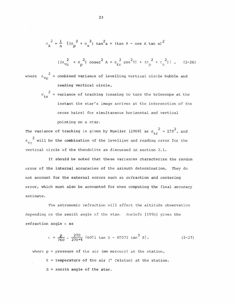
23

{ (cr 2 + a 2 ) tan2a + (tan cp - cos A' tan a) 2 p v

+ a 2 ) cosec 2 A + a 2 cos 2 ~J + (a 2 + p tr p

2 c ) } c

(2-26)

where 2

ovc = combined variance of levelling vertical circle bubble and

reading vertical circle,

variance of tracking (ceasing to turn the telescope at the

instant the star's image arrives at the intersection of the

cross hairs) for simultaneous horizontal and vertical

pointing on a star.

2 2 The variance of tracking is given by Mueller [1969] as a = 1~0 , and tr

a 2 will be the combination of the levelling and reading error for the V;;

vertical circle of the theodolite as discussed in section 2.1.

It should be noted that these variances characterize the ra.ndom

error of the internal accuracies of the azir.tUth determination. They do

not account for the external errors such as refraction and centering

error, which must also be accounted for when computing the final accuracy

estimate.

The astronomic refraction will affect the altitude observation

depending on the zenith angle of the star. Roelofs [1950) gives the

refraction angle E as

E =

where p

t

z

...£._ 760

270 {60~1 tan z- 0~072 tan3 Z}, 270+t

pressure of t!.e air (mm rnercu.::-y) at the station,

temperature of the air (° Celcius) at the station.

zenith angle of the star.

(2-27)

24

The corrected altitude a is then computed as

a=a'-E:, (2-28)

where a' =measured altitude.

Thus, the external error resul tir.g from refraction will be a result of

inaccuracies in determination of temperature and pressure. Ignoring the

last term in equation (2-27), their effect will be [Roelofs, 1950]

2 a + p <?fo 270 60"1 tan Z) 2 , 270 4- t .

where 2 a =variance of reading the barometer,

p 2

ot = variance of reading the thermometer,

and of = mean short period fluctuation in t~~perature.

(2-29)

The mean short period fluctuation-in temperature is taken as of= 0.2°C.

Equation (2-29) assumes that (2-27) is the exact model for the refraction

angle e. Although this is obviously not the case, Roelofs [1950] states

that for zenith angles less than 75°, it will be sufficiently accurate.

It must be remembered that these are astronomic azimuths, and for

obtaining geodetic azimuths a, equation (2-22) must be used. As well,

for precise work, the gravimetric, skew-normal, and normal section to

geodesic corrections must also be applied [e.g. Thomson et al., 1978]. Dracup

[1975] uses the variance

2 _ 2 (tan ¢1 ) 2 ( 0 4 a - a + o 8 + . a A • . ') 2

s~n o (2-30)

where o 2 includes both internal and external errors, and the last two A

terms are generated by the corrective terms applied to the astronomic

a~imuth to get a geodetic azimuth. Equation (2-30) is also being used

25

in the 1978/79 readjustment of the maritime second order control networks for

a priori geodetic azimuth weights [Chamberlain, 1978).

When working on a plane, the geodetic azimuth must be reduced

to the mapping plane azimuth t by subt:::acting meridian convergence y and

(T- t) corrections [e.g. Thomson et al, 1978]. Thus, any inaccuracies in y or

(T - t) must also propagate into the variance of t, i.e.

2 cr t = 2 2 2

o a+ ay + a(T-t). (2-31)

2. 4 Summary

This section summarizes the findings of the first 3 sections.

The subsections are grouped under individual observation types, and

each observation type is composed of both internal and external random

error sources. Redundant observations are also accounted for.

2.4.1 Directions

The internal va~iance for a single direction is

2 0 d.

~

= 0 p 2 + (J

r (2-32)

where the pointin~, reading, and levelling error are computed by equations

(2-1) to (2-6). From (2-19) the external error is

2 2

The variance of a single direction observation is

20 2

2 2 2 2 2 c (2-33) od = Cf + ,. + 0 + p -- . p r L 02

For n observations o= the same direction, the variance

changeSdccording to the observing procedure used. If, as is usually done,

26

the zero setting is changed between "sets" of directi.:ms, with no relevelling

or recentering of the instrument between sets, the final variance is

= (a 2 + a 2)

p r n

2 2 + 0 + p

L

2a 2 c

-y-o

(2-34)

If, however, the instrument is relevelled and recentered (after turning

instrument and targets through a 120° rotation) between sets, the final

variance is

2 2 2 2 a + 0

2 p 2c

p r ( ) + OL +

2 2 02

ad = (2-35) n 2

as there are 2 paintings and reading:> of the same direction within each

set.

2.4.2 Horizontal Angles

Ho:;:izontal angles are essent.ially the difference of 2 directio:ms.

Thus, the variance of a single angle derived from 2 single directions is

~ 2 2 2 2 2 2

.::l - 4o·

2ad 2(cr c a = = + a + r< ) + a p r ._,L

02 ( 2-36)

where the final term could be replaced by equatL>n (2-17) if it is expected

that the centering error will be an important factor.

If, as is usually done, the angles are derived from direction

observations, then n observations of an angle correspond to n observations

of 2 directions, and

is

a 2 a

the 11sual equation for the variance of angles

a 2 + a 2

2 { ....E___.E_ + a 2 + n L

2 2 '1 2 p c }

02 (2-37)

(

27

corresponding to the same observation procedure that led to equation

(2-34).

One must be careful about the covariance between angles which

are derived from a set of more than 2 directions. If the situation

exists as in Figure 2.4, then t"he angles aijk and aikl are usually

derived as

= dl..l - d. 1 .lK

Figures 2.4 Angles and Directions

(2-38)

The propagation of errors fron, the directions into the angles by the

covariance law yields the variance covariance natrix of the angles as

2 2 2

1 (J + c -o dik d .. d.k l.J L

c =

dil2 j

a (2-39) 2 2

-a '"' + ,. dik djk

28

One can see that because of the common directi.,n dik between the 2 angles,

the covariance -2 Thus, if angles are computed above, a occurs. as

dik the a priori variance covariance matrix is not diagonal, but

has the off diagonal covariance terms of minus the variance of the common

direction between individual angles.

Of course, it is possible to measure angles independently, and

in this case no covariance terms will appear in C • a

2.4.3 Zenith an?les

Zenith angles can be considered the difference of 2 directions

as well, one being defined by the vertical axis of the theodolite, the

other by the optical axis of the telescope pointed at the target.

The internal variance of a zenith angle is

2 2 2 2 a = ~ + a + a

z. v p r l.

(2-40)

2 where a is now the levellin<J error corresp01,ding to the vertical circle v

index.

The external error is

2 2 2 a

z e

=a + c;, e: ')

2 where a is given by equation (2-12}, and

e:

= . 2

Sl.n E 2

s·

(2-41)

(2-42)

for a variance aHT2 of height of target and measured zenith angle E; Combining

equations (2-40) and (2-41), and accounting for n zenith angle observations,

29

2 2 2 2

a + a + a = __ v ____ ~P~----~r--n

(2-43) Cf Z: •

if the vertical circle index is relevelled for e~ch observation. In most

2 cases, the greatest source of inaccuracy , i.s o r:

2.4.4 Astronomic Azimuths

As already discussed, astronomic azimuths can be split by

method of determination into 2 groups. F01~ gyro azimuths, the internal

variance is best calculated as the variance of the mean of repeated

determinations, arid for azimuths dr.:!termined by star observations, they

are given by equations (2-24) and (2-26),respectively. The external

error is composed of centering error and, for azimuth determination

by altitude of stars, the errc'r in determination of astronomic refraction

(equation (2-29)). Thus

= a A. ~

2 + c

rf 2

(2-44)

2 where crrf = 0 for gyro- azimuths and azimuth by hour angle of stars. The

accuracy increase for n observations is accounted for in the internal

accuracy component.

2.4.5 Geodetic Azinutl:~-

The geodetic azimuth a has further inaccuracies rr;;sulting

primarily from the random error in the prime vertical component of the

deflection of the vertical n (see equation (2-22)). An expression

such as equation (2-30) must be employed to account for these inaccuracies.

29a

2.4.6 "Grid" Azimuths

For grid or plane azimuths, equation (2-31) should be employed, I

2 . 2 2 but oy and o(T-t) are usually very small in comparison with oa In

all practical cases, the variance of the grid azimuth can be assumed

identical to that of the geodetic azimuth, namely

2 2 0 = 0

t a (2-45)

30

3. DISTANCE MEASUREMENTS

The accuracy of diftance measurements is also divided into an

internal and external compone11t. Most distances are now observed with

EDM, and the so-called zero and parts per million error are essentially

internal and external errors, respectively. Both mechanical and optical

methods of distance measurement are also considered as they are still

widely used for distance observation.

3.1 EDM

Electromagnetic distance measuring (~DM) equipment utilize

the following general equation for measured distanceS:

1 S = ~ ~ (ru + 8/2~) , (3-1)

where s == measured distance,

A modulation wavelength of frequency being used,

m = integer number of wavelengths in twice the distance,

e = phase difference between transmitted and reflect wave

in radians.

Thus, the variance of the measured distance for EDH is primarily a function

of the variance of A and 8 (m is considered known), namely:

31

= (3-2)

From equation (3-2), it is seen that the variance of determining the

modulation wavelength A contributes to the external 7ariance (distance

dependent) , and the phase difference uncertainty a:-. contributes to the

internal variance. Other sou:r:·ces of iJ.aCCUL'lc:y auch as zc.:ro error,

error in zenith angle determination, and earth curvature determination

error affect the final distance measurement, but the variance of the

observed distance is basically characterized hy equation 1"3-2).

3. 1.1 Internal

The magnitude of a~ is primarily a function of the method used ·:

to determine the phase difference 8. In older EDM instruments, a phase

discriminator circuit or CRT was used to indicate directly the difference

in phase of the transmitted and received waves. In this case, a resolution

of 0.01 of a cycle is possible [Burnside, 1971]. Instruments using null

point methods of phase comparison [e.g. Geodimeter Model 6) cw1, as a general

rule, detect a phase change of 0.001 of a cycle. The more recent digital

method of phase detection, which is used largely in the modern infra-red

equipment, gives a resolution from 0.001 up to 0.0003 of a cycle [Deumlich,

1974]. Table 3.l,from Deumlich [1974] ,points out the major features of

some of the available modern EDM equipment.

The second term in equation (3-2) i:·, due to

inaccuracy in phase determination, and is rewritten as:

2 1 2 2 crph = {2 A} oe ( 3-3)

for o 8 in fract.ions of a cycle (i.e. parts of one wavelength) .

Model I I Manufacturer Radiation

I Source

I

Geodimeter AGA 1sm\l He-NP.

~ode1 8 S1·1eden Laser Georln 1 ite 3 G Spectra-Physics I 5n;:·! He-Ne

U.S.A. j Laser Geodimeter AGA 130 H fl.ode 1 6 Sweden i:!ercury Lamp Geodimeter 76 AGA i 2mW

Sweden I Laser OM 1000 I Kern 1 GaAs-Oi ode

.. , . I " I ?,00- ~m ~,_ - L

ME 3000 o:·i soo

Si1 11

ELOI 2

~ 100

CD 6 smi-3

Oi 3

D:1-60 r.!•hi tape 3800 13

Ran~er I I

I : Y.e~n I I Zeiss

I Oberkochen Zeiss

1 Ob crkochen I Te11urometer l

Tell urometer Sokl:isila Ltd, Tokyo '4i 1 d Heerbrugg

( 100 Hz) G.1As Oi ode 875 nm GaAs Diode 910 nm

Gal',s Diode 930 nm GaAs Diode r.a!ls !Ji oc!e 900 nm Gal's Diode 875 nm

I \.11hic !nd. I SaAs Diode I r.o. , l!SA i 900 nrr:

Hewlett- GaAs I Pad:ard, t.:SA Diode

I laser Syst. & 3m!-l He-Ne Electronics USA Laser

I ' 1 " I ~Cth~' of I ""'' ( Kml I Stoodud I I Modulation Frequency I ~1odu1ator I r-ower I rlia~c I - i

Consumed (W) Measurement Day Night I Deviation Base (I~H~) I Total # I

I [._ I I

I I I

! I

I

30

49

30

15

rroro

15

15

75

15

7.5

75

15

15

I I I I '

I

4

5

3

2

2

!"

2

2

4

2

2

3

4

4

I I

l I I I !

KDP Crystal

Kerr Cell

Kerr Cell

I - I 1\nn ,.. ............. 1 I

I

KOP Crys ta 1!

I

75

. 400

70 300

11

10

i1

12

4

14

10

, " ,.,

15

12

Table 3.1 EDM Instruments

' I null meter

I digital

j reso 1 ver I null meter

I I I

digital

"n.+r.m.o.l'"h:::.n.;r::.l

nu11 meter digita1

automatic digital

digital

digital digital

digital

automatic diqital digital null meter automatic digital

I

( 3 prisms) 0.5

(3 prisms) 2

( 19 prisms) 5

2

2 1

( 3 prisms 0.6

(3 prisms} 2

3 (3 prisms)

6

:!:_ (5 rrrn + 1 • 10-6·J;)

+1.10-6s or 1 mm whichever greater :!:_(1 em+ 2.lo-6s)

-6 } :!:_(1 em+ 1.10 s

+ 1 em

-6 ' :!:_(0.2 ~~ + 1.10 s,

+ 1 cr::

+ 5 to 10 11111

+ 5 !1111

-6 ~(1.5 mm + 2.10 s)

•(r. r.;~ · ~ '0-6s' . ;J ..... .,... ..J. l I

+ l Cf.1

!(5 rnP + 5.1o-6s)

,_ + , ,0-:) ) .'!:_P r..rn '. • s,

( 1 -5 \ ::_5m.+1.0 S;

( -5 :!:_ 5mm + 2.10 s)

I

c.. "-

Antenna

14ode 1 IY1e1nufacturer Carrier Measurin~ Diameter DiverJence Frequency (GHz) Frequency MHZ) · (em) (0

MRA 101 Tellurometer Ltd. 10.05 to 10.45 7.5 33 6

MRA 3 Tellurometer Ltd. 10.025 to 10.45 7.5 33 I 9

MRA 4 Tellurometer Ltd. 34.5 to 35.1 75 33 I 2 '

CA 1000 Tellurometer Ltd. 10.1 to 10.45 19 to 25

E1ectrotape Dl-:20 Cubic Corp. U.S.A. 10.5 to 10.5 7.5 33 6 I I I

I i Distorr.at DI50 ~Ji 1 d Heerbrugg 10.2 to 10.5 ! 15 36 6 I , I

l 0~' toooa ~ D IEO __ j S; omeo,-A 16 i '"''' I ' I

I L_ !

10.3 150 35 __ j_ 6

Table 3.1 continued

Power l

Consumed Readout Measuring (w) ~ange ( Km)

38 digital 0.1 to 50

digital 0.1 to 50

digital 0.05 to 60

digital .0.05 to 30

digital 0.05 to 50

I I I 50 digital 0.1 to 50

I I !

!

I digi~- 0.02 to 150 I 38

!

Standard Deviation

. 6 ~(1.5 em+ 3.10- s)

~(1.5 em+ 3.10-65}

~(3 mm + 3.10-65)

I -6

~(1.5 em+ 5.10 s)

I ~(1 em+ 3.10-6s)

-6 ~(2 em+ 5.10 s)

-6 ~(1 em+ 3.10 s)

! I

I

I I ! I

I l I

w w

34

l''or an instrument with modulation frequency 15 MHZ (A ::. 20 m) , and a resolution

2 -4 2 o6 = 0.001 of a cycle, oph = l.lO m , or oph = 1 em.

Some instruments (e. g. the vlild DI-3) take the mean of a great

many determinations of a before employing equation (3-1) to determine the

distance. In this instance, equation (3-3) reduces to

2 1 0 = ph n

( 3-4)

where m is the number of de~erminations of the phase difference e.

From the above discussicn, it is seen that it is important

to know the value of o62 to obtain a reasonable estimate for oph2 . A

2 more accurate figure for o6 than that which can be g:2aned from the

explanation above and Table 3.1 should be available (for a s~ccific

instrument) from the manufacturer's specifications.

One other source of internal error which must be considered

is the uncertainty in the zero error cr which results from inaccurate knowledge of the z

difference between the electrical centre of the instrument and the

point used to center the instrument over the statL;n. For instruments

using light waves, this value is usually negligible, but for micro\·rave

devices, the value can be quit8 significant. The zero error is dependent

on the carrier frequency used: for instance in the MRA4 which has a

carrier wavelength of 8 rnrn, o is estimated at 3 mm, but for the MRA 101 z

(carrier wavelength of 3 ern) , cr is thought to be closer to 15 rnrn z

[Burnside, 1971]. One method for determining the zero error on a calibrated

baseline is given in Chrzanowski [1977].

35

3.1.2 External

The first term in equation (3-2) is due to the uncertainty in .the

determination of tThe modulation wavelength A· Difficulties·ari~e here

primarily due to the index of refraction n, which affects the wavelength

as

= A

0

n

where A is the wavelength resulting from 0

A 0

c f

(3-5)

(3-6)

for c =speed of light in a vacuum= 299792458 m/sec [Laurila, 1976],

and f modulation frequency being used.

Assuming A to be errorless; the variance of A is then given as 0

2 0:\ C1

r.

2 (3-7)

Substituting this result back into the first term of equation (3-2)

yields 1 A (m + G/21T) 2 0 0

{--·---::-----} 0 2 = S 2 n 2 2 n

2

(3-8)

n n

where S is the distance being observed.

The refractive index n depends on the type of carrier wave-

length used by the instrument. The two casic carrier wavelengths used

by EDM are lightwaves (infra-red is also included here) and microwaves,

2 and thus n and a are

n computed differently for these two cases.

For lightwaves, the formula of Barell and Sears is usually

used as follows [Burnside, 1971]:

where

(n-1) 273.15

= (nG-1). T p

760

36

15.02 e T

10-6 ,

T temperature in degrees Kelvin (t°C + 273.15),

P pressure of the air in mm Hg,

e = water vapour pressure in ~n Hg,

nG refractive index for the group velocity defined as

= 28760.4 ~ 488.64 + 6.80 A 2 >. 4

c c

where A = carrier frequency wavelength. For computation of e, one is c

(3-9)

(3-10)

referred to Bamford {1975 , p. 54}.Laurila [1~76] arrives at the simplication

N,.P - 41.8 e N = ... 7

(3-ll)

3.709 T

for N = (n-1) 6

NG = (nG-1).10 , and P ~nd e in millibars. When

evaluated for the effects of P, e and t, equation (3-11) gives

-N = {.!__ ( G P + 11. 27 e)} 2

T2 3.709 2 {11.27} 2

Gp + T 2

0 e

2 Thus, 0 is computed as n

(3-12)

( 3-13)

For microwaves, the group velocity is essentially equal to the car!:ier

velocity, and the Essen and Froome formula is usually employed as follows:

N = 77.62 p (12.92 T - T (3-14)

37

where T is in degrees Kelvin, P and e are in units of millibars, and

6 N = (n-1) . 10 . The propogation of variance through equation (3-14) yields

{-77.62 + (12.92 T2 T2

4 2 74.38·10 ) e} 2 crT2 +{77.62}

T3 T

4 2 +{-12.92 37.19·10 }2 2

crp + 2 cr • T T e~

(3-15)

Equation (3-15) is also due to Laurila [1976].

Table 3.2 from Kukkamaki [1967] summarizes the effects of errors

METEOROLOGICAL ERROR

+ 1 mm Hg in air pressure

+ l°C in temperature

+ l°C in the difference between dry and wet bulbs

EFFECT ON

Light Waves

0.3 ppm

1.0 ppm

0.05 ppm

DISTANCE

Microwaves

0.3 ppm

1.6 ppm

8.0 ppm

Table 3. 2 Effect of Meteorological Errors on r1easured

Distances

in meteorological measurements on the measured distance. For light ~;aves,

the most important is temperatur~ and air pressure, but for microwaves, the

difference between wet and dry bulb temperatures, which is used to compute

e, must be determined accurately.

Another external effect which cannot be overlooked is the error caused

by reducing the measured slope J.istance s (already corrected for index of

refraction and zero error) to either i) a horizontal distance Sh at the

average height of the two stations (usually the procedure for localized

surveys), or ii) the geodesic distance on a reference ellipsoidS. 0

38

Figure 3.1 [Chrzanowski, 1977) illustrates the indi•.ridual steps in the

reduction process.

Figure 3.1 Reduction of Distances

There are essentially five separate corrections which must be

considered in order to understand the errors resulting from them, and they

are defined as follows [Bom.ford, 1975) :

1. The correction for the effect of curvature of the path of the ray and

earth on the computation of the index of refraction. This correction

is given as

s m

- s = -s 3 2 (K - K ) ,

l2R2

where R = mean radius of the earth = 6370 km,

( 3-16)

and K = R/K,where K is the radius of curvature of the path of the ray

from A to B.

Under average conditions, f;=7P. for lighh;av,?s (K=l/7=0.143} and K'-= 4R

for microwaves (K=l/4=0.25}.

39

2. Reduce the path distance S to the chord or spatial distance S • The latter m s

3.

would be the distance required for a three dimensional adjustment,

and the correction is

6S 2 = S - S s r.\

s 3 __ m_ K2 •

24R2 ( 3-17)

The correction 6S 3 reduces the spatial distance Ss to the level distance

Sh at the average height of the two points. The correction is

s m

( 3-18)

where i.\h = (hB - hA) ::: difference in height between the two points.

4. The level distance Sh is reduced to the chord distance Sc at the ellipsoid

by the correction

s - s = c h

where h m

average height of the two points above the

ellipsoid,

R = Euler radius of curvature for the line. a

5. The final reduction of s to the geodesic distance S is via the correction c 0

6S =s -s 5 0 c

s 3 m

24R2

Thus, the reduced level distance sh is

and the final geodesic distance on the ellipsoid is

(3-20)

( 3-21)

( 3-2 2)

40

The effect of inaccuracies in the corrections As propagate directly

into the reduced distance sh or s 0 • By calculating a few examples, it can be

seen that for distances under 50 km, the combined correction ~s 1 + ~s 2 is

less than 1 ppm, and thus any inaccuracies in K, R, or S will not affect

the reduced distance significantly. However, the correction ~s 3 is directly

linked to the difference in height, and any uncertainty in Ah will affect

the correction L'ls 3 in the following way:

2 {L'Ih} 2 ~; tS = S

3 m (3-23)

ignoring the small contribution of the second tern (see equation (3-18)).

For instance, for a distance S = 2000m, L'lh m

100 m, and 0 6h = 0.5 m,

nt,.S 3

2.5 em.

An important consideration here, then, is the method used to

determine t.h. One of the usual methods employed is the measurement of

the vertical or zenith angles to determine t.h as

6h = S cos E , s

where E is the measured zenith distance. An error oE in the zenith

distance (see section 2.2.11 propagates as

2 0 llh = (S sin E) 2 oE 2

s .

(3-24)

(3-25)

which for a distance of 2000 m, E = 85°, and a = 20" gives cr ::. 0.2 m. 'E t.h

The correction L'ls4 will contribute an error of

2 s 2 cr = {_h }

[), s 4 R (3-26)

41

where (R + h ) in equation (3-19) has been replaced by R. m

The height

above the ellipsoid h is usually not well known due to inaccurate rn

knowledge of the geoid height N. As can be verified from formula {3-26) 1

each 6 m of error in h will contribute 1 ppm error to the reduced m

distance S . 0

3.1.3 Summary of Variance for EDM

The variance of the final r~duced distance s is summarized as r

2 (j

2 2 2 + s2 n crs = crph + a?. 2

r n

2 The value to be used for cr~ 5 depends on the type of reduced distance

2 desired. For the level distance Sh' cr 65 is equal to a6s 2 , and for

(3-27)

the ellipsoidal distance S0 , a,~ = cr 2 u b.S 3

2 3 + o65 {see equations (3-23) and

4 {3-26)). Distances to be used in a three dimensional adjustment will not

2 require a cr 65 term unless they are exceptionally long {see secticn 3.2).

To understand how the variance is affected for more than one

determination of the distance, one must first consider the normal observing

procedure. Usually, the inst~ument is set up, the zenith angle is

observed to determine 6h, the meteorological readings are taken, the distance

is observed m1 times, meteorological readings are taken again, the zenith

angle is reobserved, and the procedure is complete. In this case, the variance

of the reduced distance ~s

as r

+ cr z 2

2. ellS •

+ 2 (3-28)

Thus, the repeatedly observed distance serves only to reduce the variance

2 of phase difference determination a ph • 'I'he uncertainty in the zero error. is qr"

7 2 affected and on~ and otis are dependent on their individual measurement

procedures. In general., for m1 observatio:~s cf phase difference, m2 sets

42

of meteorological readings and m3 determinations of the height differences,

accuracy as

r cr z

2 + +

Most instrument manufacturers state their instrument's

cr = + (a + b.S) s

(3-29)

(3-30)

where a and b are the internal and external standard deviations

respectively. In the present context, a=/ cr~h + oz2 and b = on/n. One

can see that equation (3-30) is not valid, as

Equation (3-27) properly accounts for error propagation whereas equation

(3-30) does not.

3.2 Mechanical Distance Measurement

Steel surveying tapes or chains as well as invar wires and

tapes are considered here as the instr.uments used to measure distances

mechanically. The errors in these measurements are all dependent on the

distance measured, and thus are regarded as external errors.

For graduated steel tapes used with plumb bobs to determine the

vertical, Kissam [1971] reports an expected accuracy of 1:2500 with no

corrections applied, 1:3000 when using a spring balance to obtain the

corr~ct tension, and 1:5000 when the teMperature correction is also applied.

Higher accuracy measurements are usually made with the tape

suspended in catenary (see Figure 3.2). The ends of the tape are

43

T

Figure 3.2 Tape in Catenary

supported firmly and precisely (usually by means of tripods designed for

this purpose) at A and B, and a tension T (e.g. 10 Kg) is applied at A.

The tape will then "sag" by a predictable amount (proportional to its

weight per unit length, the distance between A and B, and the tension T)

and the spatial distance S ca11 be computed. .7!;. det"iled analysis is s

contained in Bamford [1975].

Clark [1969] considers an accuracy of 1:20000 easily achievable

with steel tapes in catenary which have been standardized (compared with

an accurately known length) and which are used with applicable corrections

(i.e. temperature, tension, sag and slope).

Invar wires or tapes in catenary can be used to :)btain accuracies

up to 1 to 2 ppm [Bomford, 1975]. Corrections considered necessary to

achieve this accuracy (besi~e~ those mentioned ubove) include pulley friction,

the weight of dirt or moisture on the wire or tape, the effect of wind,

and the change in gravity between the standardisation site and measurement

site. These high accuracy measurements with invar wires were primarily

used to measure baselines to introduce scale to geodetic networks before

the advent of modern EDM.

44

3.3 Optical Distance Measurement

Optical distance measurement is still an inexpensive and useful

method of distance determination, even though it has been largely replaced

by EDM. One reason for this is that the accuracy of optical distance

measurement deteriorates quickly with increasing distance, even though

relative accuracies up to 1:20000 are achievable for distances under about

500 m.

This section is based entirely on the comprehensive text "Optical

Distance Measurement" by Smith [1970], and, as such, will summarize the

main points pertaining to determination of the variance of the reduced

distance. Of the nine separat~ types of optical distance measuring

equipment covered by Smith {1970], only stadia tacheometry and subtense

bars are considered here. As can be expected, errors here are related

to those of Chapter 2 as these optical methods of distance measurement

require theodolite observations.

3.3.1 Stadia Tacheometry

This method can be used on any theodolite which has stadia

hairs. 'fhe reduced distance s1 is computed as (Figure 3. 3) "t

sh = cb cos 8 cos ~. (3-31)

where C = instrument constant for stadia hairs (ususally 100) ,

b = difference in reading between upper and lower stadia

hairs,

8 = observed vertical angle,

~ = angle between normal to line of sight and the

vertical rod.

45

Figure 3.3 Stadia ~easureMents

The angle 1jJ is not taken equal to 8 as the error a 1)1 in l1olding the rod

vertically is not the same as t-he error c',} in thP. observed vertical

angle. The error i'n the reduced distance is thus

(3-32)

where o 8 and oW are in radians and ~h is the difference in height between

the centre rod reading and the instrument stati·.J!l. The error in reading

the rod obis dependent on the pointing error (see section 2.1.1) and on the

distance of the rod from the instrument. For example, given 6h 8. 7 m,

= 100 m, o6 = 1', a,,,= lu, and ab = 0.7 mm, then a = 0.167 m, which 'f' sh

is a relative precision of 1:600.

The inaccuracy of vertical angle determination a 8 has already

been discussed in section 2.2.1, but it is obvious that ow will generally

be the largest contributing factor. It is difficult to manually hold the

rod vertically in error less than 1°, but if it could be aligned to 1',

then the relative precision for the above example would be 1:1400.

46

3.3.2 Subtense Bar

The subtense bar method does not require a vertical angle

observation; the horizontal distance is immediately available as (Figure 3.4)

b a = 2 cot 2 , (3-33}

wl1ore b len<_rth of the subtcnsr bar,

a ~ neasured horizontal angle subtended by the

sub tense bar.

The length of the barb is •,4:!11 known (e.g. ab = 0.00005 m), and the primary

source of error is cra 2 ' the variance of the measured angle. The evaluation

of cr 2 is covered in section 2.4.2. The variance of the computed a

distance is

fbr a in units of radians. a

1+------Sh---- ------Figure 3.4 Bar at End

(3-34)

Differently configured setups yield different values for o1 . s.

J If the subtense bar is set in the middle of the line as depicted in Figure

3.5, then the variance for Sh is

47

Figure 3.5 Bar in the Middle

s 20" = { h a}2 ,

212b ( 3-35)

which is 2.8 times better than for the bar at the end of the line.

Equation (3-35) assumes al = a2 and cr = a In general, for n equal al a2

segments of shape as in Figure 3.4, the error is 2

2 sh cra 2 crs = { 3/2} (3-36)

h b n

For an auxiliary base at the end of a line,as depicted in

Figure 3.6, the error in distance is

2 2 b' 2 crs = sh {- +

h b 2 (3-37)

for cra in radians. The optimum condition (least error in Sh) occurs when

Figure 3.6 Auxiliary Base at End

48

y = a (see Figure 3. 6) , and in this case

3 2 2 sh 2

(3-38) 0 sh b

0 a

for o in radians. a

When the auxiliary base is placed in the middle of the line

l.-b ... j

Figure 3.7 Auxiliary Base in the Middle of the Line

as in Figure 3.7, then

b'2 [ __ + c 2 b

s 2 h ' ---)

8b' 2

2 a

again for o in radians. Optintal conditions occur here for the ratio a

Y 2 = 12 : 1 : 1, • ··hich yields

= 25 3

h 2.8b

(3-39)

(3-40)

Figure 3.8 [Smith, 1970] shows the relative precision expected for the

four cases discussed above assuming a subtense bar of length b = 2 m.

3. 4 Sununary

This section SUiiliTiarizes the variance of the three types of

distance measurement discussed above. Each method is treated independently

of the others because of the unique nature of t!:c individual distance

determination procedures.

49

500 500

400 400

loo · 300

2.00 2.00

100 100

L----4----~----~---+----~--~s~ 0 1~2.000 it4000 1t6000 1:1000 1:10000 ~

Be1se o.t End 1:2.000 1:4000

Bttse in 1:6000 1:6000

Middle 1:10000

600

+OO

2.00

<rs 1:+000 UOOO }:J?.OOO 1:16000 {:2.0000 _h

Auxilia.r~ Ba.se in Mfddle Sh

Figure .3.8. Expected Relative Precision of Subtense

Bar Measurements

(3-29) as

so

For ED.M distances, the fina-l variance is given by equation

= a z

2 +

2 where a65 depends on the type of reduced distance required (see section

3.1.3), o 2 is computed by equation (3-12) or (3-15) depending on the carrier n

frequency wavelength, o 2 is either given by the manufacturer or determined z

through a calibration procedure, o~h is determined from equation (3-3)

•-:r (3-4), and rn1 , m2 and m3 are as explained in section 3.1. 3.

The variance of mechanical methods of distance observation is

characterized by (3-39)

where o5 is the relative pre,-:ision of the method heing used (see section m

3.2). For example, consider taping carried out with plumb bobs and no

corn~ctions applied for tension or temperature;

and for a measured distance of 500 m, os = 0.2 m.

then cr 2 = (1/2500) 2 , s

m

Optically determined distances have a variance whict. is

highly dependent on the individual method used. For stadia tacheometry,

equation (3-32) characterizes the variance, and for subtense bar measurements,

equations (3-34), (3-35), (3-38) and (3-40) define the variances depending

on the specific subtense method used. 2 Each of these formulae depend on cr a

(the variance of angle determinatim:) which is given by equation (2-37).

51

REFERENC:::S

Angus-Leppan, P.V. 1961. Study of Refraction in the Lower Atmosphere. Empire Survey Review, Vol. XVI, ·~os. 120, 121 and 122.

Angus-Leppan, P.V. 1971. Meteorological Physics Applied to the Calculation of Refraction Corrections. Paper, Commonwealth Survey Officers Conference.

Bamford, G. 1975. Geodesy. London: Oxford University Press.

Burnside, C.D. 1971. Electromagnetic Distance Measurement. London: Crosby Lockwood Staples.

Carter, W.B.,J.E. Petty, and W.E. Strange. 1978. The ~ccuracy of Astronomic Azimuth Determinations. Bulletin Geodesique, Vol. 52, no. 2.

Chamberlain, C.A.M. 1977. l1athematical Hodels for Horizontal Geodetic Networks. Technical Report no. 43, Dept. of Surveying Engineering, University of New Brunswick, Fredericton.

Ch~mberlain, C.A.M. 1978. Personal Communication.

Chrzanow~;ki, A. 1977. Design and Error Analysis of Surveying Projects. Lecture Notes no. 47, Dept. of Surveyi~~-ngineering, University of New Brunswick, Fredericton.

Clark, D. 1969. Plane and Geodetic Surveying for Engineer~. Vol. l, Plane Surveying,Sixth ed. London: Constable and Co-Ltd.

Cooper, M.A. R. 1971. Modern Theodo_.!.i t:_es and Lcve ls. London : Crosby Lockwood & Son Ltd.

Deumlich, F. 1974. Ins~~en~enkunde der V~~essungstecr1ni_~· Berlin: VEB Verlag fur Bauwesen.

Dracup, J.F. 1975. Use of Doppler Positions to Control Classical Geodet.ic Networks. Paper, International Association of Geodesy, XVI General Assembly, Grenoble.

Faig, w. 1972. Advanced Surveying I. Lecture Notes no. 27, Dept. o~ Surveying EngineeriE.S_, University of New Brunswick,. Fredericton.

Gregerson, L.F. 1974. Using Gyrotheodolites for Precise Determination of Azimuth. Internal Report, Geodetic Survey of Canada.

Halmos, F. 1977. High Precision Measurement and Evaluation Method for Azimuth Determination with Gyro-theodolites. J~a~u~~rip~a

Geodetica, Vol. 2, no. 3, p. 213.

Kissam, P. 1971. Surveying Practice. Second ed. New York: McGra•w Hill.

52

Kukkamaki, T .. J. 1949. 011 Li1t:eral R.:'fra.ction in Triangulation. _!3ulletir~

Geodesique, no. 11.

Kukkamaki, T.J. 1967. Geodet1c Refraction, Vertical Horizontal and Longitudinal. International Dictionary of Geophysics. London: Pergamon Press.

Laurila, s. H. 1976. Electron i.e Surveyi~nd Navigation. New York: John Wiley & Sons.

Mepham, M.P. 1976. A Rigorous Derivation of Station Adjustment Formulae for Complete and Incomplete Sets. Report for SE 4711, Dept. of Surveying Engineerin.:I.!... University of tlew Brunswick, Fredericton.

Mepham, M.P. 1977. Short Line Trigonometric LcvPlling. Rep:nt for SE 3701 Qept. __ o.!_~~L~~- Engi_nc~i_ng, University of Nc•.v Brunswick, Fredericton.

Mueller, I. I. Spherical and Pr:act i.£_~!_ __ ~st;:o~()_El_}'_ as Applied ~)2odeS'(· New York: Frederick Ungar Publishing Co.

Pfeifer, L. 1975. Use of Ferrero's Formula to Estimate a Priori Variance of Horizontal Directions. Paper, J Venezuelan Congress of Geodesy, Maracaibo.

Ramsayer, K. 1978. The Accuracy of the Determination of Terrestrial Refraction from Reciprocal Zenith Angles. Paper, IAU Symposium 89, Refractional Influences in Astrometry and Geodesy, Uppsala.

Robbins, A.R. 1976. Military Engineering. Vol XIII, Part IX, Geodetic Astronomy. Ministry of .Defense.

Field and

Roelofs, R. 1950. Ast~__y App_lie~_!:_£ __ ~c:_n_<:'!__:'2._U}"_V~-Yi_!:l3.· Amsterdam: N. V. Wed. J. Ahrend & Zoon.

Smith, J.R. 1970. Optical Distan~--~eas~~~~-~~- London: Crosby Lockwood & Son Ltd.

Thomson, D.B., E.J. Krakiwsky and J.R.. Adams. ,\Manual for Geodetic Position Computations in the Maritime Provinces. Technical Report no. 52. Dept. of Surveyjng_ Engi':!_eering_, Uni vel-s i ty of New Brunswick, Fredericton.

Vincenty, T. 1973. Three-Dimensional 2\djustmer;t of Gc:odetic Networks. Internal Report, D~1i\AC GPodet ic Survey Squadron.