Techniques of Water-Resources Investigations of the United States Geological Survey

Chapter A4

A MODULAR FINITE-ELEMENT MODEL (MODFE) FOR AREAL AND AXISYMMETRIC GROUND-WATER FLOW PROBLEMS,

PART 2: DERIVATION OF FINITE-ELEMENT EQUATIONS AND COMPARISONS WITH ANALYTICAL SOLUTIONS

By Richard L. Cooley

Book 6 Chapter A4 b

Therefore, the

cRi = & ReAe. i

final leakage function is

H. - + 2QHi r + 1 - + t 1 n !%Hi , n+l "f;: Hi.n n+.l 5 'hi,n 2Qhi,n 1

h A

3 h i.n+l - hi,n * + ?hi,n+l Atn+l i,n - hi,n 1 I + $ Hi n+l - 'i n+l 3 , 11

Q mi,n'

M1(TiAtn+ll 7i '

M2biAtn+lj 7i '

'hi,n+l Atn+l + 'Ri

H. 'Hi,n + 2QHi,n 1 - $Hi n+l ' nit

- Hi.n 9 n+l

1 + 5 'hi,n + 2Qhi,n - $Ri[Hi,n - 'i,n [ , I 1

+ 2 Hi n+l - ii n , I] (206)

(203)

(204)

(205)

The leakage process described by equation (206) is time dependent, but linear. Therefore, equation (206) is added into equation (58), unless the predictor-corrector method is required to include other phenomena, in which case equation (206) is added into the appropriate predictor and corrector equations. The coefficient of 6i is added into l for every node i where

leakage occurs, side.

and the remaining terms are subtracted from the right-hand

FINITE-ELEMENT FORMULA TION IN AXISYMMETRIC CYLINDRICAL COORDINATES

GOVERNINGFLOWEQUATIONANDBOUNDARYCONDITIONS Axially symmetric ground-water flow in an aquifer is assumed to be

governed by the following unsteady-state flow equation written in axisymmetric cylindrical coordinates (Bear, '1979, p. 116):

(207)

64

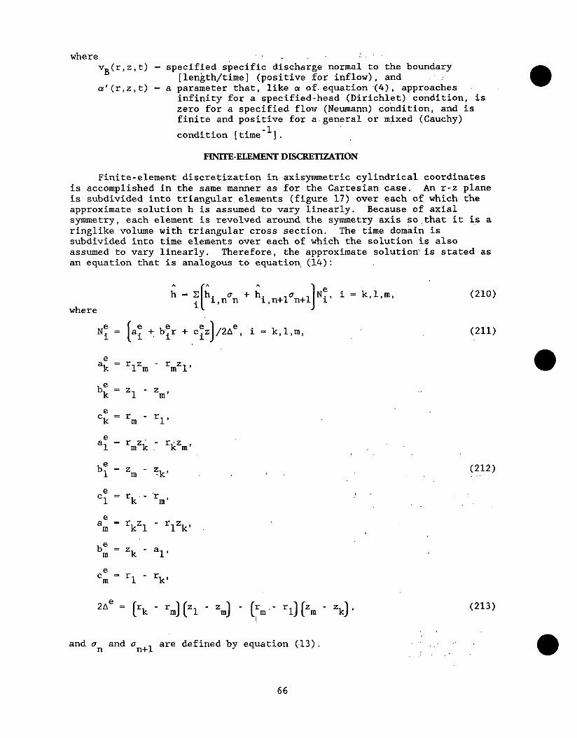
Figure 17. Axisymmetric aquifer subdivided into spatial finite elements.

where the new symbols used are

r = radial (horizontal) coordinate direction [length] from the axis of symmetry, which is vertical,

z = vertical coordinate direction [length], Krr(r,z),KZZ(r,z) = the principal components of the hydraulic conductivity

tensor [length/time] in the radial and vertical coordinate directions, respectively, and

Ss(r,z) = specific storage [length -1 1.

The orientation of the r and z axes is shown in figure 17.

The principal directions of the hydraulic conductivity tensor are assumed to be parallel to the r and z axes in equation (207). Equation (207) was not written in full component form like equation (l), because any rotation of the principal directions from the r and z axes (see figure 5) must be revolved around the z axis to maintain axial symmetry. This pro- duces the physically unusual case of an axially symmetric rotation of the principal directions, which seemed to the author to be an unnecessary complication to include.

Equation (207) is subject to boundary and initial conditions analogous to equations (2) through (5) used for equation (1). However, equations (3) and (4) must be changed to reflect the change from flow integrated over aquifer thickness in equation (1) to flow in a radial cross-section in equa- tion (207). Thus, equation (3), which expresses flow continuity across a discontinuity in the porous medium, is replaced by

(208)

where v,(r,z,t) is the normal component of specific discharge, and equation

(4), which expresses either a specified-head or Cauchy-type boundary condition, is replaced by

V n = vB + a'(Hb - h), (209)

65

where . . . ;. . vB(r,z,t) - specified specific discharge normal to the boundary

[length/time] (positive for inflow), and : a'(r,z,t) - a parameter that, like a of-equation (4), approaches

infinity for a specified-head (Dirichlet) condition, is zero for a specified flow (Neumann) condition, and is finite and positive for a-general or m$xed (Cauchy)

condition [time -1 1.

FINITE-ELEMENT DISCEETIZATION

Finite-element discretization in axisymmetric cylindrical coordinates is accomplished in the same manner as for the Cartesian case. An r-z plane is subdivided into triangular,elements (figure 17) over each of. which the. approximate solution h is assumed to vary linearly. Because of axial symmetry, each element is revolved around the symmetry axis so?that it ir; a ringlike volume with triangular cross section. The time'domain is subdivided into time elements over each of which the solution is also assumed to vary linearly. Therefore, the approximate solution is stated as an equation that is analogous to equation, (l.4):

where

E; = C ii L i '

nan + ii , n+lan+l

1

’ NY, i = k,l,m,

NT = a: + bfr + c:z /2Ae, i = k,l,m, I

a: = rlzm - rmzl,

b; = zl - zm,

c: = rm - rl,

a: = rmzk _- rkzm,

b"l = zm - zk,

CT = rk,- ‘rm,

e a m = rkzl - rlzk,

bi = zk - al,

e C =r -1: m 1 k'

(210)

(211)

zl-z rl)(Zm - 'k]'

.’ .(212)

.

J

(213)

and u and (T n n+l are defined by equation (,13).

66

DERIVATION OF FINITE-ELEMENT EQUATIONS

The error-functional equation in axisymmetric cylindrical coordinates is analogous to equation (15). It is written for an r-z plane as

(214)

Minimization of equation (214) with respect to ii n+l and separation of the 9

result into two parts as for equation (17) gives t n+l B r ii u

ei 0 n+l

he I[ NYSs

i aNf a;l aN; a;l at + F Krr Z + Z K~z Z 1 rdrdz

:J

P

-lc?[vB + CY'(H~ - G)]rd( lJ[ N;Ss 2 + 2 Krr e

he

1

+ $ KZz E]rdrdz - lCc[vB + a'(HB - h)]rdC

I

dt' - 0. (215)

By following the procedures used in appendix A, the second part of equation (215) can be shown to equal zero. Therefore, when the integrals

involving Ssai/at and a'(HB - ;I) are converted to diagonal form using

approximations analogous to equation (19), the following integral form of the finite-element equations results:

di.aNe "aNe A 2 + 2 Krr g + ti KZz 2 1 rdrdz

11 rdC dt'

] = 0, i = 1,2,...,N. (216)

Equation (216) is analogous to equation (21). However, because the principal axes of the hydraulic conductivity tensor were originally assumed to be parallel to the r and z coordinate axes, no coordinate rotations are performed.

67

Equation (216) is integrated to obtain the final finite-element equations. As before, the spatial integrations are performed first. It is assumed that Ss, Krr, and Kzz are all constant in each spatial element, and

that vB and a' are constant along any Cauchy-type boundary side of each

element. The extra r in the integrals presents a complication not present for the Cartesian case. However, by writing, r as the identity

r = Ner + Ner + Ner kk 11 mm' (217)

equations (24) and (25) can be used to perform the integrations. Therefore,

by substituting the appropriate expressions for h, NY, aNy/ar, and aNT/az,

i = k,l,m, the spatial integrals in equation (216) are evaluated for i = k (for example) as-

d;lk

1

d;l NESs Frdrdz = $3: 2rk + rl + rm Ae2,

aN;A aNe* Khl +-$nm rdrdz

I

KL =- 4Ae

+ b;b;;ll+ b;b;hrn 1 r,

K" h h h =zz ceceh kkk + ceceh + ceceh

4Ae kll 'k m m

N;[vB + d(HBk - ik)]rdC = i(2rk + + (afL]kl(HBk - hk;i2')

(218)

(219) l

II aN; h

ii7 Key a2 &rdrdz =

he

rdrdz

+ tkrk + 'm][pBL)km + ~r14)km[HBk - ‘k]] (221)

where S E, Kzr, and Kzz are the constant values of S s, Krr, and KZz in element e,

rm 1

, (222)

and other terms were defined earlier.

68

The spatially integrated finite-element equation for node k is obtained by substituting equations (218) through (221) into equation (216) and using equations analogous to equations (41) and (42). The result is

- :[[2rk + rl)pBL)kl + [2rk + rm](vBL)km] - :[[2rk + rl>("'L]kl

+ c 2rk + r

31 II } m a'L km HBk dt' = 0, (223)

where

CEk = hSi 2rk + rl + rm he, 1

VEk = :[[2rk + rl)p'L)kl + [2rk + 'm)pfL)km]'

t& = -& -

gEl =

gEm=

(224)

(225)

(226)

(227)

(228)

As before, equation (223) must apply to all N nodes of the finite-element mesh. These N equations are written in matrix form as equation (45), where C V..,andG ij' LJ

ij are given by equations (47) through (49), and

2r +r i j '] [pBL)ij'

Specified-head boundaries are handled using

To perform the final time integration,

are all assumed to be constant in time, and

ij

equation (51).

(229)

parameters Ss, K,,, KZZ, and a'

specified boundary flux vB is

assumed to be linearly variable through each time element. Thus, the time

integrated finite-element equations for axisymmetric flow are given by equation (58) with B replaced by B defined by equation (62). No nonlinear or other extensions-are used. -

69

FINITE-ELEMENT FORMULATION FOR STEADY-STATE FLOW

By definition, steady-state flow occurs when hydraulic heads do not vary with time, or ah/at = 0 in equation (1) or (207). Steady-state flow equations are obtained by setting S or Ss to zero and letting all quantities

in equations (1) through (4) or (207) through (209) be time invariant.

LINEARCASE

The finite-element equations for steady-state confined flow in the absence of any of the nonlinear source-sink functions may be derived from

equation (56) by setting g (which contains S or Ss) to zero and setting cn+l

-;I -;1 -n -' The resulting equation is

(230)

where A - G + V. As for unsteady flow, round-off error may be minimized by solvinE foT hezd change rather than head. Thus, by defining this head change, (To, as

6 - ii - IJo' -0 - (231) h

where ho is an arbitrary initial set of heads close to h, equation (230) is

modified to become Ato = f - go- (232)

To solve a linear, steady-state flow problem, first equation (232) is solved

for 6 -o, then equation (231) is solved for i. Mass balance components are

obtained from equation (232) using analogous procedures to those used for unsteady-state flow.

NO- CASE

If steady-state flow is unconfined or a nonlinear source-sink function h

is employed, then & and B are functions of h and a nonlinear problem results. In the case of-unconfined flow, an off-diagonal entry of c is

given by equation (74) in which bi = ii - Zbi' The particular form of the

nonlinear source-sink term incorporated into V and B is dependent on the type of function: point head-dependent dischzrge, area1 head-dependent leakage, area1 head-dependent discharge, or line head-dependent leakage.

The general algorithm used to solve the nonlinear problem is derived before stating the specific terms used for unconfined flow and nonlinear sources and sinks. For nonlinear problems, equation (230) is restated as

(233)

where the notation 4 are functions of i _-

An iterative solution method for equation (233) may be derived by adding and

70

subtracting $ 5 iI

to the right-hand side, then restating the'result 'as, an

iteration equation of the form

or

where R is the iteration index, and

(234’)’

(235)

(236)

(237)

(238)

Head-change vector ts in equation (234) frequently requires damping to ,

reduce undesirable oscillations from one iteration to the next. Addition of a damping parameter pR (0 < pR I 1) to equation (237) yields the following

iteration algorithm: h

1

rJ = BjJ - cQ!J -1

5 = 41 ?iJ I = O,l,... (239)

sp+l

h = PJSJ + ??Jj

The iterations are terminated when

max 6 R I I i I c i S’

'(240)

R where hi is a component of en and es is a small number about an order of h

magnitude smaller than the desired accuracy in h.

An effective empirical scheme for computing pg was developed by Cooley:

(1983, p. 1274). It is given in three steps. Let eR be the value of 6:

that is largest in absolute value for all i = 1,2,...,N, and let emax be the largest value of eR

I I permitted on any iteration. Then,

Step 1.

el P'

%leR-l' R>l

p=l ,R=l

(242)

Step 2

3+ P*=3+p , pr -1 -T-r P*y& ', p< -1

71

Step 3

pQ=P*, P*eQ 5emax I I

pQ = H , P*leQl > emax

(243)

h A good trial value for emax is about half the maximum value of

I h -0i - h -i I

expected (where hoi is a component of the initial head vector). Much

smaller values may be needed for highly nonlinear problems.

At the beginning of each iteration Q,

using the newly computed values of <Q.

AQ and E5Q must be recomputed

The way in which AQ and F5Q are

recomputed depends on the source of the nonlinearity. Nonlinearity from A

unconfined flow results when hi <

unconfined flow, off-diagonals of for iteration Q as

'ti' To allow

$ are computed

for the possibility of

from equation (74) written

where

GQ = ij

bQ = bQ-l i i ’ PQ6i Q-1, iif <

“0

b; = zti - 'bi , h; L

(244)

'ti

'ti (245)

Nodes that go dry are treated in the same manner as explained for unsteady-state flow. The head is allowed to decline below the base of the aquifer at a dry node i, but horizontal flow in the aquifer is allowed between adjacent nodes i and j unless node j also goes dry. If a dry node i becomes surrounded by dry nodes during the iterative solution process, then G ii = 0 and flow can only take place vertically through an underlying

confining unit or across a Cauchy-type boundary at the dry node. If there is no confining unit or Cauchy-type boundary so that Vii is also zero, then

A ii' which is G ii + 'ii' is zero so that the head at node i is undefined and

must be removed from the solution. This is accomplished by setting Aii to

1030 and setting the right-hand side of the equation to zero, which holds the head constant at the last computed value.. If the sum of the known fluxes is negative at a dry node, this sum is reduced by l/2 at each iteration until the node remains saturated. As discussed earlier, this tells the user the approximate discharge that can be sustained at the node.

Nonlinear source-sink functions require reevaluation of !JQ and BQ, For

point head-dependent discharge functions, reevaluation is based on equation (106) written for iteration Q as

Q~i =

_ ;;Q+l i I

, ;1f > z pi

) t; I z pi

(246)

72

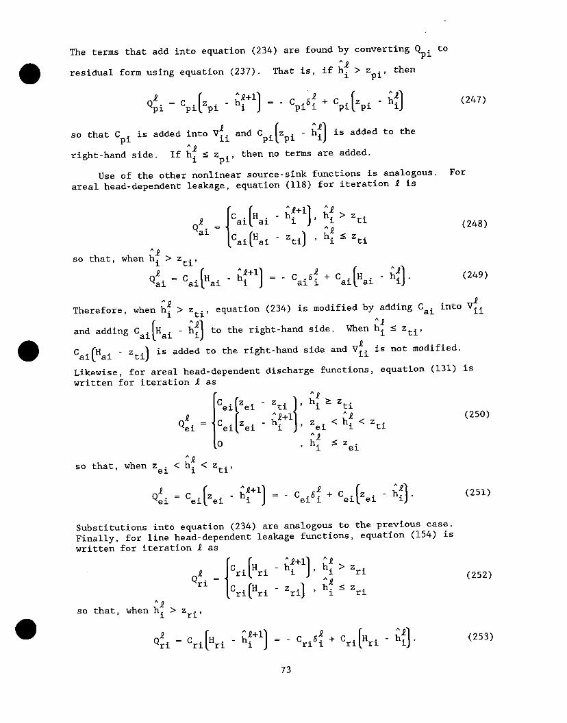
The terms that add into equation (234) are found by converting Bi to

residual form using equation (237). That is, ^R if hi > z pi' then

pi['pi (247)

so that C pi

is added into Vfi and Cpi[zpi - '13 is added to the

right-hand side. If ;l"i I z pi' then no terms are added.

Use of the other nonlinear source-sink functions is analogous. For area1 head-dependent leakage, equation (118) for iteration R is

QR 1 , i"i > Zti

ai Z , ;I", I zti (248)

^R so that, when hi > zti,

1 = - CaiS: + Cai (249)

equation (234) is modified by adding Cai into Vfi

to the right-hand side. When ;14 I zti,

C is not modified. ai c

Hai - zti 1

is added to the right-hand side and Vfi

Likewise, for area1 head-dependent discharge functions, equation (131) is written for iteration R as

(250)

so that, when z

(251) = - Cei6"i + Cei [Zei - if].

Substitutions into equation (234) are analogous to the previous case. Finally, for line head-dependent leakage functions, equation (154) is written for iteration R as

pi =

so that, when hi > zri,

1 = - Cri6; + Cri [Hri - $1.

(252)

(253)

73

SOLUTION OF MATRM EQUATIONS

Some of the symbols used in previous sections are redefined in this section to avoid complex or nonstandard matrix-solution terminology. Thus, symbols defined in this section are for use in this section only.

DEFIhTTION OF MATRIX EQUATION

Equation (58) must be solved for each time level of a linear, unsteady- state flow problem, and equations (76) and (80) (the predictor-corrector equations) must be solved sequentially at each time level of a nonlinear, unsteady-state flow problem. Likewise, equation (232) must be solved for a linear, steady-state flow problem, and equation (234) must be solved for each iteration of a nonlinear, steady-state flow problem. All of these equations are linear and of the form

Ax = d, =- (254)

where definitions of the coefficient matrix A, the known vector d, and the unknown vector x depend on the equation beinE solved. equation (58), -

For example, for

C = 4 = (2/3)Atn+l -+ $ + 2% (255)

5 = s, (256)

d=B- - _ (257)

Thus, b is an N x N matrix, and x and d are N-vectors. -

The location of nonzero entries in matrix & depends on the finite- element mesh. Each row i of 4 contains nonzero entries only corresponding to nodes in the patch of elements for node i. Therefore, unless N is very small, 4 is sparse in that most entries in any row are zero. Also, if the nodes are numbered so that the difference between the largest and smallest node numbers in the patch is small compared to N, then A is banded, which means that all nonzero entries in each row are clustere=d near the main diagonal. Because 4 is derived from the positive definite forms in equation (15) or (214), it is symmetric and positive definite. Finally, as discussed previously, if all internal angles of the spatial elements are acute, A is a Stieltjes matrix. Additional information on finite-element matrices c% be found in Desai and Abel (1972, chap. 2).

If node i is a specified-head node, equation i of equation (254) is

x. = - 1 'i,n 1 for unsteady-state flow and xi - HBi - hi for steady-

state flow. Because xi is known at all specified-head nodes, all of the

corresponding equations may be eliminated from equation (254). This may be accomplished as a partitioning operation by numbering all specified-head nodes in the finite-element mesh last, which is accomplished automatically in the code. Terms in the remaining equations that contain values of xi for

the specified-head nodes are then transferred to the right-hand sides of these equations to become part of the known vector. In the remainder of this section, equation (254) is regarded as the reduced equation resulting from this partitioning operation.

74

SYMMETRIC-DOOLITTLE METHOD

The first of two alternative matrix-solution procedures is discussed ir this section. This method is referred to as symmetric-Doolittle decomposi- tion (Fox, 1965, p. 99-102, 104-105) and is generally the preferred direct solution method for finite-element equations (Desai and Abel, 1972, p. 21). It is a direct method because the solution is found directly in three steps as opposed to iteratively in an unspecified number of steps required by the second method. Direct solution is usually efficient whenever there are fewer than about 500 nodes (Gambolati and Volpi, 1982).

The symmetric-Doolittle method is based on the fact that the symmetric matrix b can be uniquely factored into the product of three matrices (Fox, 1965, p. lOS), so that

& = UTDU = EC' (258)

where superscript T stands for transpose, 2 is upper triangular of the form

g=

‘31 Y2 Y3

0 o22 u23

0 0 o33 . . .

0 0 0

and g is diagonal of the form

l/all 0 0

0 w22 0

0 0 l/e33 . . .

0 0 0

. . . YN

. . . U2N

. . . U3N '

. . . "NN_

. . . 0

. . . 0

. . . 0

. . . l’aNN

(259)

(260)

Factorization, which is the first step of the three-step solution, is

accomplished by forming the product matrix UTDE, setting each entry of this matrix equal to the corresponding entry of 9, = =fhen solving for the unknown values of u.. and Q

1J ii' entry by entry.

Solution of equation (254) using the factorization given by equation (258) is accomplished as follows. By defining a vector y by

gx = Y' ._ (261)

the combination of equations (254) and (258) can be written as

gTgy = d* (262)

The lower triangular form of gTD and the upper triangular form of g permit equations (262) and (261) to eazily be solved for y and x, respectively, as the second and third steps of the solution procedure. By forming the

product UTDy, it can be seen that the first equation in equation (262) contains=oziy yl as an unknown, the second yl and y2, and so forth, so that

75

the first equation may be solved for yl, which is used in the second to

solve for y2, and so forth. Solution vector x is found in exactly the

opposite way. The last equation in equation (261) contains only the last unknown, x N' the second from the last xN and x N-l' and so forth, so that the

last equation is solved for xN, which is used in the second from the last to solve for x N-l' and so forth.

For N equations with N unknown values in x, the calculations may be stated in algorithmic form as

i-l .

Qii - aii - kEl Uki"kilakk

i-l u =a..- kf1 uki"kj'akk

i = 1,2,...,N ij 13 j = i+l,i+2,...,N,

u! . 1J

= u../a.. 1J 11

i-l yi = di - kEl ukiyk

1

i = 1,2,...,N,

Yi = Yi/aii

i = N,N-l,...,l.

(263)

(264)

(265)

Equation (263) is known as the factorization step, equation (264) is the forward substitution step, and equation (265) is the backward substitution step.

When the above algorithm is applied to the banded matrix A, entries in 2 outside of the band are always found to be zero. However, g has mostly nonzero entries within the band, even if the corresponding entries in A are mostly zeros. Therefore, the algorithm can be coded to operate on and=store only entries within the band. Storage of k for efficient computer application of the solution algorithm is explained in part 3.

As with any direct solution method, the above method can generate inaccurate solutions for poorly conditioned equation systems, such as can occur when 4 is not diagonally dominant, or has weak diagonal dominance, and(or) has highly variable entries. Matrix 4 can have weak diagonal dominance if all internal angles in spatial elements are acute but R, S, and a in equations (1) and (4) (or Ss and a’ in equations (207) and (209)) are

zero and there are few specified-head nodes. Matrix A may not be diagonally dominant if R, S, and a are zero, and one or more elezents has an obtuse internal angle. Entries in A can be highly variable if values of transmissivity or element shgpes are highly variable. An inaccurate solution generally results in a large mass imbalance.

76

MODIFIED INCOMPLETE-CHOLJZSKi’ CONJUGATE-GRADIENT’ METHOD

If N is large or the direct solution method produces large mass balance errors, then an iterative method should be used. An iterative solution method called the generalized conjugate-gradient method (GCGM) has been found by Gambolati and Volpi (1982) to be more efficient than the direct method for solving sets of finite-element equations when N 1 500. The iterative method used here is a combination of a variant of GCGM by Manteuffel (1980) with a preconditioning method by Wong (1979) designed to enhance the convergence rate.

Generalized conjugate-gradient method

The iteration equation for the GCGM method is derived by replacing k with a coefficient matrix g that is similar to & but much easier to invert (Concus and others, 1975). Matrix EJ, known as a preconditioning matrix, is defined from the fact that f! can always be split into the sum of two matrices, 5 and i (Varga, 1962, p. 87-93), so that

9=g+g. (266)

Therefore, because the combination of equations (254) and (266) gives

the iteration equation is

or, written in residual form,

where

(269)

(270)

The GCGM algorithm based on iteration equation (269) can be stated as (Concus and others, 1975, p. 7-8)

Sk k = 0,

T

Bk= T Sk :k

t

k = 1,2,...,

Sk-1 fk-1

(271)

pk = Sk + &!k-l I

77

T Sk :k

ok= T e&k

1 k = 0,1,2,...,

Equations (271) can be derived using the idea that, if a set of linearly independent vectors pk, k = 1,2,...,N, can be obtained, then the

solution x can be written as a linear combination of the pk's because this

set of vectors spans the N-dimensional space. Such a set of linearly independent vectors can be obtained by constructing them to be A-conjugate,

that is, so that p?Ap. 1= J

= 0 if and only if i # j (Beckman, 1967, p. 63).

Coefficients pk are calculated to construct this set of vectors. The proper

linear combination of the pk vectors to give the solution x is obtained by

minimizing the error in the solution along the line x -k + aPk at each itera-

tion (Beckman, 1967, p. 64). The value of "a" that minimizes this error is given by ak.

In the absence of round-off error, the exact solution x is obtained in N iterations. Thus, if nearly N iterations were actually needed to obtain a good approximation of x, the method would not be useful for large systems of equations. Concus and others (1975) argued that the method can be considered to be a general iteration method that permits the gradual loss of A-orthogonality from round-off error and never converges to the exact

solution. They showed that the weighted error function [? - ?k] Tk[? - $1

is reduced at each iteration if g and 5 are symmetric and positive definite, and that the method has certain optimality properties, so that, for a good choice of G, it usually converges to the desired accuracy in far fewer than N iterations.

Modified incomplete-Cholesky factorization

Modified incomplete-Cholesky factorization is an extension of a method introduced by Meijerink and van der Vorst (1977) known as incomplete- Cholesky factorizati0n.l The extension is a combination of methods from Wong (1979) and Manteuffel (1980).

Wong's (1979) method, known as row-sums agreement factorization, is developed from incomplete-Cholesky factorization as follows. Let matrix entries located at (i,:) be those entries corresponding to nonzero entries of A, excget

and let g be an upper triangular matrix with the same form as g, that thg only nonzero entries of E are located at (i,i). Finally,

let g be a diagonal matrix with the same form as E. Then an approximate (incomplete) factorization of E is defined by

'Meijerink and van der Vorst (1977) used an approximate factorization that is more like the synxnetric-Dolittle method than the Cholesky method. However, it is still called incomplete-Cholesky factorization.

78

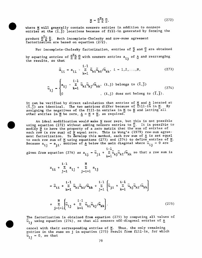
g = ETg 4, (272)

where M will generally contain nonzero entries in addition to nonzero entriez at the (T,J) locations because of fill-in generated by forming the

product ET6 fi. Both incomplete-Cholesky and row-sums agreement factorizatTog are based on equation (272).

For incomplete-Cholesky factorization, entries of p and 4 are obtained

by equating entries of CT5 8 with nonzero entries a E = =

of b and rearranging the results, so that ij

i-l a ii = a.. - 11 kzl si"ki/Gkk, i = 1,2,...,N,

i-l a.. -

ii ij =

iJ kfl %Ukj"kk' (i,j) belongs to (?,z) (274)

0 , (i,j) does not belong to (?,j).

It can be verified by direct calculation that entries of E and k located at (?,J) are identical. The two matrices differ because of Fill-in in g. By assigning the negatives of the fill-in entries in g to f3 and letting all other entries in N be zero, 9 = M + N, as required. =

An ideal modification would make ; near zero, but this is not possible using equation (272) without adding nonzero entries to g. It is possible to modify N to have the property of a zero matrix that the sum of entries of = each row (a row sum) of N equal zero. This is Wong's (1979) row-sum agree- ment factorization. To develop this method, each row sum of 5 is set equal to each row sum of M using equations (273) and (274) to define entries of g. Because a.. = a..

=J J=' &tries of & below the main diagonal where u.. = 0 are

iJ i-l

given from equation (274) as a.. = G.. + E - iJ Ji k_,ukj%i/"kk so that a row sum is

i-l N a ii + C a.. + X a..

j=l ‘J j-i+1 iJ

i-l i-l i-l cr

-- - = ii + kzl Uki"ki'Qkk + .' u

J=l I ji + kzl Ukj'ki/"kk 1 (275)

The factorization is obtained from equation (275) by computing all values of u ij using equation (274), so that all nonzero off-diagonal entries of 5

cancel with their corresponding entries of 2. Thus, the only remaining entries in the sums on j in equation (275) result from fill-in, for which ii ij = 0, so that

79

. i-l N a ii = a. ii + >: %+ci/'kk ,j=l + c f ji + ' fij' j=i+l

where f.. iJ

is a fill-in entry of g defined lby

f ij =

;kisj/&kk, (i,j) does not belong to (i,j)

, (i,j) belongs to (x,-j).

Diagonal entry z iiis calculated from equation (276) as

i-l i-l N a. ii = a.. -

11 kzl %i%i/'kk - jElfji - j=f+lfij'

(277)

(278)

Comparison of equations (273) and (278) shows that diagonal entries of & no longer equal diagonal entries of 5 defined by equation (272).

The method from Manteuffel (1980) forces ; to be positive definite, as required by the generalized conjugate-gradient method. If 4 is not a Stieltjes matrix, then E as defined using incomplete-Cholesky factorization may not be Eositive definite (Meijerink andl van der Vorst, 1977), which means that a ii computed by equation (273) will not be positive. In this

case, M as computed for row-sums agreement factorization also may not be positi;e definite because Qii calculated using (278) may be even smaller.

Manteuffel (1980) showed that computation of z ii~ 0 for incomplete-Cholesky

factorization of finite-element matrices can be prevented by adding the product of an empirically determined, small positive number, 6, and aii to

the right-hand side of equation (273). The analogous modification of equation (278) is

i-l i-l N

Qii = (1 + G)aii - ,&;ki;ki/akk - c f.. - j=l J' j=F+lfi.li *

(279)

The matrix approximately factored by this modification of row-sums agreement factorization is thus 4 + 6f (where 2 is the identity matrix), which is more diagonally dominant than &.

The above method is implemented here as follows. If Gii _( 0 is

detected during factorization, then factorization is stopped and a new value of 6, 6new' is computed from the old value, 6 old' using the empirical

equation 6 new = +&old + 0.001, (280)

where the initial value of Sold is zero. Factorization is then reinitiated,

and equation (280) is applied again if aii 51 0 is detected again, and so

forth. This process is continued until a large enough value of S is computed that all aii > 0.

80

Gustafsson (1978, 1979) also presented a method that yields equations having forms similar to those of equations (274), (277), and (279). However, his method applies to finite-difference approximations for which A is a Stieltjes matrix so that the motivation and method of choosing 6 are different.

Based on equation (272), the solution of equation (269) is obtained using the forward and backward substitution steps of the symmetric-Doolittle method as

ET& = $9 (281)

where entries of 5 and p are computed using equations (274) and (279), respectively. The remaining part of the algorithm implied by equations (281) is

-1 U ij =ii /a ij ii' (i,j) belongs to (x,5), (282)

y: = r: - i-l

jf?lciiy' i = 1,2,. . . J,

yik = ypGii 1

k ,k N

s.=y. - c 1 1 i = N,N-l,...,l. R=i+l

(283)

(284)

In _applying the above algorithm, note that the factorization step to compute g and g is only done once before applying the generalized conjugate- gradient algorithm (equations (271)). At each iteration, sk is computed

using only equations (283) and (284). The factorization, forward substitution, and backward substitution steps are all fast and require little computer storage because D is sparse like A. This combination of GCGM and modified incomplete-ChoTesky factorizatizn is called the modified incomplete-Cholesky conjugate-gradient method (MICCG method).

Stopping criteria

One stopping criterion is to terminate the algorithm whenever the

maximum value of I xk+l k

i - x i I

becomes small

k+l _ xk max x. i I 1 i I

= max i

where x k k i is an entry. of xkl pi is an entry Of pk* and E is a small positive

number, such as 10 -4 . The value of max i xk+l - xk is usually assumed to be i I i I

, or whenever

k I I akPi ' ', (285)

a rough measure of the error max in the solution. However, the

81

conjugate-gradient algorithm can sometimes yield a value of max i I

k+l _ xk xi i I

that is small even when the solution is inaccurate. Thus, another criterion

that is also a rough measure of max i Ixi - xii is employed.

The residual given by equation (270) can be written for any row i as

ail[xl - x:] + ai2[x2 - x';] + . . . + aiN[xN - x:] = rt

Thus, because aii is positive,

Ia LLJ il a. ii

x1 - x;I + J-$lx2 - xy + . . ,, + J-$IXN

or

N

k "N I

The sum C a.. /aii is i=l I I =J

generally in the range of 1 to 2, so is assumed to

(286)

(287)

(288)

J -

be unity. Therefore, a rough measure of max

additional stopping criterion is

j- lxi - x21 is Irrl/aii, and the

max r i I I t /aii 5 e. (289)

Note that if MICCG is used to solve the nonlinear equation (234), then there will be an inner MICCG iteration loop and an outer loop on the nonlinearity. An efficient way of employing MICCG for these problems is to set the convergence criterion E to be larger than normal (say, larger than es by about an order of magnitude) to reduce the number of inner iterations

taken at each outer iteration. Good accuracy is achieved by requiring close convergence of the outer iteration sequence.

COMPARISONS OF NUMERICAL RESULTS WITH ANALYTICAL SOLUTIONS

Results of simulating some simple ground-water flow problems for which analytical solutions have been presented in the literature are given here to demonstrate the accuracy of the finite-element code (MODFE). Each simula- tion is designed to test specific computational features that were discussed in preceding sections and to verify that MODFE can accurately represent the physical processes. To demonstrate that any consistent system of units may be used with MODFE, both English and metric systems of units are used in the example problems.

THEIS SOLUTION OF UNSTEADY RADIAL FLOW TO A PUMPED WELL

MODFE is used with axisymmetric cylindrical coordinates to compute unsteady flow to a well located in a confined nonleaky aquifer having homo- geneous and isotropic hydraulic properties and an infinite area1 extent.

82