Design and Control of an High Maneuverability Remotely Operated Vehicle withMulti-Degree of Freedom Thrusters.

by

Daniel G. Walker

SUBMITTED TO THE DEPARTMENT OF MECHANICAL ENGINEERING IN PARTIALFULFILLMENT OF THE REQUIREMENTS FOR THE DEGREE OF

BACHELOR OF SCIENCEAT THE

MASSACHUSETTS INSTITUTE OF TECHNOLOGY

June 2005

© 2005 Daniel G. Walker. All rights Reserved

MASSACHUSETfS INSiR[JTEOF TECHNOLOGY

LJUN 08200BRARIES5

LIBRARIES

The author hereby grants to MIT permission to reproduce and to distribute publicly paper andelectronic copies of this theses document in part or in whole.

Signature of Author ...... ...- , '. ....................Department of Mechanical Engineering

May 6, 2005

Certified by .........................................................................................................Franz Hover

Principal Research EngineerThesis Supervisor

Accepted by ................................................ ...............Ernest Cravahlo

Professor of Mechanical EngineeringChairman, Undergraduate Thesis Committee

.. Vs, 1

Design and Control of a High Maneuverability Remotely Operated Vehicle withMulti-Degree of Freedom Thrusters.

by

Daniel G. Walker

Submitted to the Department of Mechanical Engineeringon May 6, 2005 in Partial Fulfillment of the Requirements forthe degree of Bachelor of Science in Mechanical Engineering

ABSTRACT

3

This research involves the design, manufacture, and testing of a small, <I m3 , < 10kg, low cost,unmanned submersible. High maneuverability in the ROV as achieved through a high thrust-to-mass ratio in all directions. One identified solution is moving the primary thrusters in both thepitch and yaw directions. The robot is propelled by a pair of 2 DOF thrusters, and is directlycontrolled in heave, surge, sway, yaw, and roll. Pitch is controlled through passive buoyancyand, potentially, active manipulation of added mass and gyroscopic effects. This system iscompared against a traditional fixed-thruster system in terms of cost, size, weight, and high/lowspeed performance. Preliminary results indicate that the actuated system can provide animproved thrust-to-mass metric at the expense of increased system complexity. This margin ofimprovement increases with increasing thruster size. The system has applications in highaccuracy positioning areas such as ship hull inspection, recovery, and exploration.

Thesis Supervisor: Franz HoverTitle: Principal Research Engineer

2

Acknowledgements

The author would like to thank Franz Hover, Tom Consi, The MIT ROV Team, The Departmentformerly known as Ocean Engineering, and the Ocean Engineering Teaching Laboratory fortheir continued support, as well as Analog Devices for the donation of accelerometers and rategyros.

3

Table of Contents

ABSTRACT ..................................................................................................................................... 2Acknowledgem ents ......................................................................................................................... 3Table of Contents ............................................................................................................................ 4Table of Figures .............................................................................................................................. 6Table of Tables ............................................................................................................................... 71.0 Introduction ............................................................................................................................... 8

1.1 Background ................................................................................................................... 81.2 Relevance of this Problem .......................................................................................... 101.3 Outline ......................................................................................................................... 11

2.0 M echanical Design .................................................................................................................. 122.0.1 Quantitative Analysis ................................................................................... 122.0.2 Iteration of Designs ...................................................................................... 15

2.1 Developed M echanical Design ................................................................................... 212.2 Thruster Design ........................................................................................................... 22

2.2.1 Thruster Implementation Overview ............................................................. 232.2.2 Front Spindle ................................................................................................ 232.2.3 M otor M ount ................................................................................................ 252.2.4 M otor Selection ............................................................................................ 26

2.3 Pitch Actuator ............................................................................................................. 272.3.1. Structure ...................................................................................................... 272.3.2. Drive System ............................................................................................... 28

2.4 Yaw Actuator .............................................................................................................. 302.4.1. Structure ...................................................................................................... 302.4.2. Drive System ............................................................................................... 31

2.5 Body ............................................................................................................................ 312.5.1 Anhedral Connector ..................................................................................... 312.5.2 Ballast and Floatation .................................................................................. 32

3.0 Control System Design ........................................................................................................... 343.1 M echanism Servo Control .......................................................................................... 34

3.1.1 Com pensator Design .................................................................................... 383.2 Kinem atic Controller .................................................................................................. 39

3.2.1 Analysis ........................................................................................................ 393.2.2 Low Level Algorithm .................................................................................. 423.2.3 Advanced Algorithm .................................................................................... 43

3.3 User Interface .............................................................................................................. 443.4 Controller Hardware ................................................................................................... 44

4.0 Experim ental Validation ......................................................................................................... 464.1.0 Single Mechanism: Setup and Procedure .................................................... 464.1.1 Single M echanism : Results .......................................................................... 474.2.0 ROV Mount: Setup and Procedure ............................................................. 504.2.2 ROV M ount: Results .................................................................................... 51

:5.0 Analysis / Discussion .............................................................................................................. 526.0 Conclusion .............................................................................................................................. 54Appendix A: Control System Schem atics ..................................................................................... 55

4

Appendix B: Control System Code ............................................................................................... 58

5

Table of Figures

Figure 1: VideoRay Scout [ ]........................................................................................................... 9Figure 2: Sebotix [BV . .............................................................................................................. l0Figure 2: Sebotix LBV [2].10

Figure 3: Degrees of Freedom for a Free-Flying Robot .............................................................. 12Figure 4: Principal Coordinate Systems and Thruster/Actuator Implementations ....................... 16Figure 5: Selected Fixed Thruster Configurations: ....................................................................... 17Figure 6: Two Single Degree of Freedom Thrusters .................................................................... 17Figure 7: Hybrid Thruster - Surface Port ROV ............................................................................ 19Figure 8: ROV with a Pair of Two Degree of Freedom Thrusters ............................................... 20Figure 9: Concentric ring mount ................................................................................................... 21Figure 10: Experimental Implementation of ROV Design ........................................................... 22Figure 11: Section view of Front Spindle ..................................................................................... 24Figure 12: Section View of M otor M ount .................................................................................... 26Figure 13: Load Cases .................................................................................................................. 27Figure 14: Section View of Pitch Actuator ................................................................................... 29Figure 15: Section View of Yaw M echanism ............................................................................... 30Figure 16: Anhedral Connector .................................................................................................... 32Figure 17: Ballast and Flotation Righting M oments ..................................................................... 33Figure 18: Control System Architecture ....................................................................................... 34Figure 19: Torque-Speed Curve for Copal Gearmotor HG16-030AA []...................................... 35Figure 20: Voltage Controlled DC M otor Block Diagram [1 ....................................................... 36Figure 21: Output Compliance M odel .......................................................................................... 36Figure 22: Servomechanism Control System Block Diagram ...................................................... 37Figure 23: Reduced Feedback Loop ............................................................................................. 38Figure 24: Coordinate Systems ..................................................................................................... 40Figure 25: Visual Basic Control ................................................................................................... 44Figure 26: Control System M ain Board ........................................................................................ 45Figure 27: Robot mounted on test stand ....................................................................................... 46Figure 28: Servomechansim test setup for water .......................................................................... 47Figure 29: Low frequency input and system response. 30 cycles = 0.6 Hz ................................. 48Figure 30: High frequency input and associated magnitude decrease. 6 cycles = 2Hz ............... 48Figure 31: System Response in Air .............................................................................................. 49Figure 32: System Response in W ater .......................................................................................... 50

6

Table of Tables

Table 1: Drag Forces on an ROV Hull ......................................................................................... 13Table 2: Strategy Level Design ..................................................................................................... 20Table 3: Thruster Efficiency ......................................................................................................... 26Table 4: Servomechanism Parameters .......................................................................................... 38Table 5: Control Hardware Requirements and Implementation ................................................... 45Table 6: ROV Performance v. Initial Specs .................................................................................. 52

7

1.0 Introduction

The overarching purpose of this research is to extend the current field of high maneuverabilityunderwater robots. This is an attempt to create a new ROV based on design principles, ratherthan existing designs. The initial bias is towards a more complex system, as there are already anumber of commercially available, relatively simple ROVs.

The robot in this research should be small and highly maneuverable. High maneuverability willbe defined as the ability to: hover in one place; adjust position or velocity without turning first;and quickly change direction.

In order to adjust position without turning, the ROV must have active control of every directionin which it is expected to move. For a small inspection-class ROV, the ability to translate in anydirection greatly enhances the product usability. Most ROVs of this type have a front camera andgripper payload. The ability to move laterally allows the user to precisely position the ROVpayload. User control of pitch and roll are not required for this ROV. This will limit theoperations to inspecting mostly vertical walls. The ROV can still be used on complex hullforms, but it will not be able to maintain a constant, normal orientation to the surface.

In order to adjust position or accelerate rapidly, it is desirable to have as little system mass aspossible, while having the maximum output force from the thrusters. This is a basic applicationof Newton's second law. Confounding this, however, stability also effects the systemperformance. Stability is the system's ability to withstand disturbance inputs. High stabilitymakes precise positioning easier for the user, and is desirable. For this attribute, increased massis desirable, as a larger mass is more difficult to accelerate by outside forces. However, a similareffect can also be achieved with a more complex control system. The tradeoff here appears to beincreased complexity in the control system versus a more sluggish response. Because the controlsystem can be improved later with less effort than reducing mass in the mechanism, a lightersystem is selected.

For an actively controlled system, the system should be as small as possible, with thrusters asforceful as possible. For a passive system, the system should be as large as possible, withproportionally larger thrusters.

The generation of numerical specs is somewhat arbitrary, but is loosely based on numbers 1-2Xbetter those from commercially available ROVs, such as those covered in the next sections. TheROV should be approximately 1 ft3, have a max speed 5 m/s, be able to change velocity fromlm/s to -lm/s in 1 second, and have a mass of 5kg.

1.1 Background

Unmanned underwater vehicles (UUVs) can generally be divided into long-range and short-range machines. The long-range machines have slender hulls, shaped like a torpedo or modernmilitary submarine. They also usually rely on one large propeller with a series of rudders andcontrol surfaces. These are designed to travel long distances efficiently, and are generally used

8

for surveying and mapping of large grids in the ocean. The short-range vehicles are more box-like, and have multiple thrusters. These robots are designed to move in several differentdirections from a standstill. By comparison, the long range robots can only change directionwhile they are moving. The short-range robots are used in applications such as object recovery,hull inspection, and diver assistance.

In clarification of commonly used acronyms, autonomous underwater vehicles (AUVs) aregenerally considered to be robots without a tether. Remotely operated vehicles, on the otherhand, do have a tether. In industry, AUVs are used to perform long-range tasks, while ROVs areused to perform short-range tasks. Within the prototypical applications, the ROV/AUVdefinition is logical. However, there are a number of instances where the industry conventioncan become misaligned with the definition of the acronym. For example, a robot that is remotelycontrolled by radio or acoustic methods may still be considered an AUV, although it is notautonomous. Classically, remote control is not practical unless using a tether; remote control byacoustic or radio transmissions rarely have the necessary range or bandwidth, so a tether is used.This paper will hold to the industry convention, with clarification as needed.

There are a number of small, maneuverable ROVs on the market. The two most widely usedones, with dry weight less than 25 lbs, are the VideoRay and LBV.

The VideoRay Scout is the smallest platform sold by VideoRay LLC. It has a maximum depthrating of 91m, max speed of 1.9 knots, mass of 3.6 kg, dimensions of 0.35x0.25x0.21m, andcosts $5,995.00 including controls and monitors. Higher-end models have greater depth rating,speeds to 2.57 knots, and more operational sensors and accessories. All are based on a threethruster design, with two forward thrusters on the sides, and one vertical thruster in the center. [ l

The Sebotix LVB is a similar system made by Cetrax Systems LTD. A 150m rated system startsat $16,182.87 [converted from pounds]. The LBV has 4 thrusters: two forward thrusters, avertical thruster, and a lateral thruster, for top speeds of 2 knots vertically or laterally, and 4knots forward. The LBV is larger than the Scout, measuring 0.49x0.26x0.24m and 10kg.Higher end models have depth capacity up to 3,500m [2 ]

9

Figure 2: Sebotix LBV 121

1.2 Relevance of this Problem

One of the traditional applications for underwater vehicles it the mapping of the ocean floor. Inaddition to basic cartographic data, high resolution sensors can help locate wreckage andarchaeological remains. The vehicle typically flies a regular pattern over the floor, takingelevation data as it passes overhead.

Another application for highly maneuverable ROVs is ship hull inspection. This can be part ofregularly scheduled preventative maintenance, damage assessment, or searching for contrabands.The VideoRay is already used in searching the ballast tanks of large vessels, saving the cost anddanger of draining the tanks or sending in divers. In addition, increased security concernswarrant the inspection of large LNG carriers for attached mines or explosive devices.Commercially available software allows for the detection of anomalies on previously mappedhulls while using a small ROV.

Work-class ROVs can also augment or replace divers for light repairs or coarse manipulation oftools and objects.

The deep oceans are relatively unknown when compared to dry land, or even parts of space. Amajor contributor to this is the lack of ROVs for ocean-going scientists. For deep submergence,the number of capable ROVs or Human Operated Vehicles is still very small. The NationalResearch Council has identified deep submergence assets as an inadequately met need.However, the development of new ROVs or restructuring of current assets would have asignificant cost. [3] The pressure and hostility of the deep waster environment immediatelyexcludes any researcher without access to such a high-end ROV or HOV. Thus ROVs are abasic tool for any such deepwater research.

10

-

1.3 Outline

This paper, after the current introduction, analyzes the problem first from a global view. Basicengineering parameters such as power, response time, and geometry are generated from theinitial specifications. Next, an overarching design is created to meet these parameters. Eachrelevant subsystem is designed and analyzed. Next, the system is tested, and performance ismeasured and compared to the initial specifications. Lastly, conclusions are drawn and futurework is discussed.

11

2.0 Mechanical Design

In a free-flying ROV, the principle axes of motion are surge, sway, heave, pitch, yaw, and roll.

Figure 3: Degrees of Freedom for a Free-Flying Robot

Thruster power is initially suspected as the most sensitive parameter in determining the size andperformance of an ROV. Electronics are small and generally constant in size. Power can besupplied through the tether. The only other main component, the payload, creates theperformance specifications directly through mass and lift capabilities. Also, payload createsperformance specifications indirectly through setting the mission type, such as being highlymaneuverable for a hull inspection camera, or having efficient propulsion for long-durationsonar scanning. At the small end of the ROV range, mechanical overhead such as wiring,pressure housings, and structural members also start to play a role in ROV form.

2.0.1 Quantitative Analysis

In order to create a design for the proposed system, the initial suspicion of the thruster as mostsensitive parameter is assumed to be correct. Different aspects of the performance specificationsare analyzed in terms of the necessary thruster power. A series of different thruster arrangementsare created to fulfill the thruster power requirement. Lastly, the arrangements are compared andthe suspicion is validated.

The power required from the thrusters are in terms of the total fluid power, and do not considerefficiency losses from the propeller and drive train. These factors are considered during motorselection in section 2.2.4.

The drag force F on the ROV is determined by the coefficient of drag, Cd, the surface area, A,and the free stream velocity, U.

12

Heave

Y

Yaw

C

i

Pitch

(..Sway

u RollSurge

F. =C AU2 (1.1)

The drag coefficient is empirically determined using the above relation. where the Reynoldsnumber is a relation between the fluid density p, velocity, U, characteristic length, L, and fluidviscosity t.

Re= pUL (1.2)

The Reynolds number for an 0.3m object in water moving at 1 m/s is 3x105, putting the flow inthe critical regime.

For initial estimates, the ROV will be modeled as somewhere between a sphere in the laminarregime and a cube. The Cd sphere is then inversely proportional to the Reynolds number forReynolds numbers less than 102, and approximately 0.5 for Reynolds Numbers less than 105.[4]

24Cd sphere low R (1.3)

- - Re (1.3)

Cd _spherehigh 0.5

The Cd for a cube is accepted as 1.05 [ 5 for Reynolds numbers greater than 1 0 . Assuming afrontal surface area of 0. lm2 (-1 ft2), or an equivalent diameter of 0.35m, the drag forces arelisted in table 1. Assuming that Pwater = 103; twater = 10- 3

Table 1: Dra2 Forces on an ROV HullGeometric Model Drag Equation Drag at Drag at Drag at Drag at

U = 0.2 m/s U = O.5 m/s U = 1 m/s U = 5 m/sSphere Low Speed 24 14water (A = 0.1 )U 6.85e-7N 1.71e-6N 3e-6N

2Pwater(D = 0.35)Sphere High Speed (Cd = 0.5)(A = 0.1)U 2 .001 N .00625 N .025 N 0.6875 N

Cube (C = .05)(A = 0.1)U 2 .0021 N .0131 N .0525 N 1.3125 N(C =l0)A01) 2.01

Using the upper bound cubic model, the max steady-state speed for ROV is a function of themaximum mechanical power output for the thruster motors

Pmaxmotors Fdrag (v) V.max

= 1.05 .0 V2 .V.,max motors 21.05 . max

(1.4)._ 3maxmotors

Vmax 0.0525

To achieve the initially specified max speed of 5 m/s, the thrusters must be capable of supplying

Pmax motors =.0525V 3 = 6.56W (1.5)

13

i

i

i

i

Drag may limit the performance of the ROV for the specified requirements. For comparison,momentum effects will be examined. The maximum required power output for the motor is rateof energy change required to move the system. Initial requirements specified a change invelocity from m/s to -l m/s in 1 second.

Pma motor = dWmechanical = dEmechanical (1.6)-rnaxd mtrdt dt

Emecanical = Epotential + Ekinetic 17

Emecanical = 2 mv 2 + 2

Because the system is neutrally buoyant, gravitational potential and buoyancy potential energycancel, leaving only kinetic terms. With constant system mass, the power is

Paxmotor = (m d V2 +I -co2) (1.8)- (m2 dt dt

Assuming a constant acceleration profile, the specified acceleration requirement is 2m/s 2. Ifrotation is held constant, the motion can be modeled as a linear velocity profile.

v := 1-2t

Pmax motor =¥m (1-2) 2 =¥_ Piax motor = d (1-2t)2 md (1-4t+4t2) = m(-2 + 4t) =-2ma. (1.9)

Pr)ax motor = 2' 2m = 20W in air

However, underwater, an additional added mass term must be added in order to account forwater that is accelerated along with the moving body. Using the cube model for the ROV, theadded mass is calculated by summing added mass coefficients over the width of the body. For acube of side length L

mlI =l.5DrpL [6] (1.10)

madded = f1.5 l pdw04

madded =1.51 p = 1186L = 50.8kg (1.11)

4The maximum thruster power will now be significantly greater. Revising Eqn 1.8The maximum thruster power will now be significantly greater. Revising Eqn 1.8

14

Pmax motor| = 4(m + madded) = 4(5 + 50.8) 220W in water (1.12)

By examining the contributions of drag and momentum to the power requirements, it is seen thatthe drag specification is less than three percent of the total power requirement. Momentumeffects dominate. In order to fulfill the initial specification, however, the ROV must be able togenerate this much power in each of the four desired degrees of freedom: surge, sway, heave,and yaw. This is nontrivial.

2.0.2 Iteration of Designs

The previous section developed the requirement for a large power output in each of the fourcontrolled directions. An iterative process is used to create and downselect designs.

In order to generate power in the three translation directions, a thruster must be pointed in thatdirection at the time of motion. This can be accomplished by a fixed thruster pointed in thedirection, or a movable thruster oriented temporarily in that direction. Because the robot movesin all three orthogonal translation directions, the minimum number of fixed thrusters is three.With three orthogonal fixed thrusters, however, the ROV is capable of translating along anyvector in the three dimensional space (R3). Such a fixed-thruster ROV has the ability toimmediately generate a translation thrust vector in any direction.

Translation may also be implemented by using thrusters that can move in one or more directions.The minimum number of moving components to achieve 3D translation is three. A singlethruster is moved in two orthogonal directions can produce the full space. For a non-over-actuated system (no redundancy), translation components can be thought of as specialcoordinates. (Fig. 4) Pure translation is possible only when the thrust vector intersects orextends from the center of mass. In the coordinate system analogy, the origin is the center ofmass. In this light, the three fixed thrusters are a Cartesian implementation, with magnitudes inSurge - X, Sway - Y, and Heave - Z. Similarly, the single thruster with double actuation can beseen as a spherical implementation. The thruster magnitude provides the radius R, while stackedrotation in latitudinal and longitudinal provides the angles and 0. Using this discovery toiterate, it is seen that a hybrid system between pure magnitude and rotation can be used: thecylindrical coordinate system. Two thrusters are implemented: a single fixed thruster in theheave - Z direction, and another thruster actuated in a plane normal to the first thruster,providing R from the thruster magnitude and 0 from the angle.

15

Hecve

Figure 4: Principal Coordinate Systems and Thruster/Actuator Implementations: (a) Cartesian (b) spherical(c) cylindrical

None of the above systems are capable of producing rotation, however. One additional thrusteror actuator must be added in order to achieve the fourth degree of freedom: yaw. For thisrotation, the thrust vector must now not intersect or extend from the center of mass. Continuingwith exactly-actuated systems, the two boundary designs are apparent. First, using one thrusterthat is free to move in three directions. Such a design would be a complex combination oftranslation and rotary actuators. Second, using fixed thrusters: three thrusters are configured asbefore in the Cartesian arrangement, with an additional thruster parallel to the X or surgethruster, but out of line with the center of mass. A variant on this design is to have two thrustersequidistant from the center of mass. This configuration is found on the LBV. Using reciprocity,however, it is seen that the additional thruster can be anywhere within the XY plane, as long asthe thrust vector does not intersect the center of mass. Most conveniently, the alternativeconfiguration has the additional thruster parallel to the Y thruster. This is comprised of twolateral thrusters and one forward thruster..

Having the two thrusters pointed in the same direction provides the benefit of having twice thethrust capability. This means that smaller thrusters can be used, or additional performance canbe gained. Because this is highly desirable, a similar configuration is sought for the two singlethrusters. By rotating them 45 , the pair of thrusters is still able to generate a thrust vectoranywhere in the YZ plane. In order to generate thrust in the principle directions, however, boththrusters must contribute. To move in the heave (Z) direction, both thrusters must turn on thesame direction. To move laterally in the sway (Y) direction, the thrusters must operate inopposite directions: one pulls while the other pushes. The benefit comes with the vector additionof the thrust. Each thruster contributes a projection on the principal axes:

Fz = sin(45°) ruster sin(135 ) thruster2 (1.13)

Fz max =l.41 4 Fthruster max

Fy = cos( 4 5 °) Fthrsterl cos(13 5 ) (-Fthrster2 )(1.14)F max = 1.414M .hruster -rmax(1.14)

F¥_ ax =--l'4 14'-Fthruster max

16

Hecave Hcae

Surge(b),_;

Z Thmtei

Sway

Act at

Stzge (C)

In this arrangement, the maximum thrust developed in both directions is nearly one and a halftimes larger than having both thrusters inline with the principle axes. The cost to the system is inthe lost energy from the thrust that cancels out. Twice as much power is required for less thanone and a half times the output.

(a) (b)Figure 5: Selected Fixed Thruster Configurations: (a) Orthogonal (b) Vertical V

In between the boundary designs (4 fixed; 1 3dof), there are also a number of designs. Althoughthe implementations may vary, the topology is limited to three cases: two fixed thrusters and one1 dof thruster; 1 fixed and one 2dof thruster; two 1 dof thrusters. Within these topologies, anumber of designs were developed. Most interesting of these is for an ROV with two thrusters,1 dof each. (Fig 6) In this design, one actuated thruster is located inline with the center of mass,providing heave or sway motion, depending on the orientation. The second thruster is actuated inan orthogonal direction, and is located away from the center of mass. When inline with thecenter of mass, the second thruster provides surge motion. When orthogonal to the center ofmass, the second thruster provides yaw rotation.

Thruster 1:

+y1

-X

c asLs

Figure 6: Two Single Degree of Freedom Thrusters

+Z

17

\ !

I.. ..... ... ....... ........... . ......... ....... .......................... ..... ......-. ....... ..... .. .... .......... ............ .....I.......... ...... _-- ........ ..........-. .... ............... -_.._..._....___.._.._._..1 ....

Applying reciprocity, over-actuated systems are now analyzed. In an over-actuated system, thenumber of actuators exceeds the desired degrees of freedom. These systems are characterized bymultiple configurations capable of achieving the same total output vector. This can bebeneficial, by allowing the system multiple options to achieve a commanded output.Presumably, one potential configuration will be closer to the current configuration than the other,allowing a faster realization of the command. The control system required to handle this,however, is considerably more complex.

Going to the extreme, we look at possibility of highly over-actuated systems. One design,casually suggested by Dr. Hover during brainstorming, is an robot using surface jets. The designwould incorporate thrusting elements over the entire surface of the robot. In oneimplementation, tubes on the surface would be connected to a central manifold and pumpingsystem. Movement is achieved by pumping in fluid from one half, and pumping out on theother. Rotation could be achieved by integrating surface ports that are not inline with the centerof mass: shear thrusters, as it were. With proper design and selection of ports, such a designcould be capable of putting out full power in any direction.

Simplifying this idea, but continuing with the same general mechanism, is a robot incorporatinga limited number movable surface ports with a central pump. This trades the complexity of themanifold system for the complexity of actuated nozzles at the surface. In order to prevent theneed for a manifold, the nozzles are designed to have an 'off position within the actuation range.This design could also be capable of full power in any direction.

Thrusters are proven components with relatively high efficiencies. A hybrid system isconsidered by incorporating both thruster and surface port technology. One implementation isconsidered in detail. (Fig 7) The robot is given a primary direction. Along this axis, a combinedthruster/pump mechanism is located. Intakes on both ends of the robot are used to draw in waterfor the surface nozzles. By switching the direction of one of the intakes, water flows in oneintake and out the other. This acts as a thruster, and propels the vehicle most efficiently in theprimary direction. By switching this output back to an intake again, water is forced out throughthe surface nozzles, allowing lateral, vertical, rotary, or combined motions. This design initiallyappears best suited for fast motion in one direction, with slower positioning and steering in theother directions.

18

Figure 7: Hybrid Thruster - Surface Port ROV

Moving back to pure thruster-actuator systems, a number of over-actuated systems are examined.First and simplest is a robot using redundant fixed thrusters. For example, an ROV could usetwo or four vertical thrusters. These could be used to actively control pitch and roll. While theuser does not provide input data for these two axes, the computer uses sensors to activelymaintain a level orientation. A simpler, over-actuated, arrangement, is to simply send identicalcontrol signals to each vertical thruster. The geometry of the robot may make such anarrangement more convenient by allowing fewer thrusters directly inline with the center of mass;only the summed vector from the vertical thrusters must intersect the center of mass. For aheavy lifting mission, it is also desirable to have more vertical thrusters, and so more verticalpower. On the opposite end, using a number of smaller thrusters may be less costly than a singlelarge thruster, depending on the thruster design.

Recalling the fixed-V design, a similar design is sought in an over-actuated family. Eachthruster should be able to contribute to multiple directions of motion. In order to overcome thepower loss from canceling forces, each of the two V-thrusters is actuated, allowing rotation inthe roll direction. This allows each thruster to point upwards or sideways for maximum thrust inthat direction. The surge/yaw thruster pair remains the same.

In a different design, the surge/yaw thruster pair is replaced by another degree of freedom oneach V-thruster. The ROV now has only two thrusters, each capable of moving in full sphericalcoordinates. (Fig. 8) This design allows each thruster to point in the direction of travel.Neglecting hydrodynamic effects, this design is capable of moving at maximum power in anydirection. This arrangement allows for direct control of five principal directions: surge, sway,

19

heave, yaw, and roll. Pitch is coaxial with the thruster pair in the figure implementation; theROV cannot pitch because the thrusters have no moment arm in the necessary direction. Acomplex use of gyroscopic and added mass would have to be used to control this axis. For a setthruster size, additional power can be added with additional thrusters. Adding a third or fourththruster also allows for direct control over pitch.

Figure 8: ROV with a Pair of Two Degree of Freedom Thrusters

Leading contenders are selected for evaluation by their relative effectiveness, efficiency, andnovelty. The main identified advantages and disadvantages are tabulated below.

Table 2: Strategy Level DesignDesign Advantages4 fixed V Conventional style design incorporates readily

available components with existingconfigurations.

2 x 2 dof Maximum thrust available in all directions.Uses existing thruster technology.

Surface port Occupies the least continuous space on thesurface area. This allows for more sensors,manipulators, and payload to be on theoutside. Uses only one high-power actuator(potentially)

Hybrid Modifies existing technology to create a newSurface Port variant on propulsion. Retains high

speed/efficiency capabilities of thruster withlow surface area overhead of surface port.Uses few high-power actuators

DisadvantagesRelatively large wasted power output andunused thrust capability

Relies on a potentially complex arrangementof bearings structures and actuators.Replaces complexity in thrusters forcomplexity in valves, pumps, and switches.

Potential for large inefficiencies. May notwork. Incorporated complexities of boththruster-based and surface-port based.

Analysis of thruster count on system performance:

The first hypothesis is that the mechanisms and structure necessary to create an actuated thrusterare negligible compared the thruster itself. This should become increasingly true with thrustersize An actuator for a small mechanism must be built to withstand the same collision forces as a

20

...

,''l ........... ...........-.........-...................--............... .. ----- _- .1...... -- .1 - ............ --- I-.,--,

large mechanism. (e.g. a 1/4" strut is much more significant to a "1/4 diameter actuator than to a 3"diameter actuator) Thus, small actuators will be overbuilt for operational loads, or those causedby the thruster. A larger actuator has less overhead, as the operational loads are closer tocollision loads. In addition, more materials must be used relative to size for the small actuator toaccommodate the fixed sized components, such as seals, o-rings, mounting surfaces, andbearings. While special exotic components can combat this, using them will increase systemcost.

Although the scaling argument seems to follow logically, it does not prove that the actuatormechanism becomes negligible within a useful range of sizes.

The 2 x 2 design is selected, as it has the potential for drastic performance improvement, whilestill using existing and proven technology.

2.1 Developed Mechanical Design

After selecting the twin 2dof thruster design, detailed design for the mechanisms was required.The robot is divided by function into four assemblies: thruster, pitch actuator, yaw actuator, andbody. The thruster creates the force which propels the robot through the water. The pitch andyaw actuators implement the two degrees of freedom specified. The body holds everythingtogether.

In examining the possibilities for two rotary axes, two seemingly different options appeared.First is the pan and tilt mechanism, typically involving a rotary table and a yoke. Second is amechanism with concentric rings. [fig.9]. The concentric ring approach has the advantage ofworking away from the singularity. In the yoke configuration, the system is singular whenpointing up. This means that the one of the axes is no longer able to change the position of theoutput part. In this case, the only differential motion possible is from the yoke. When thethruster is pointing up in the ring configuration, both axes can move the thruster for a full rangeof differential motion.

Figure 9: Concentric ring mount

21

Upon further inspection of the topology, however, it is discovered that the two designs areidentical, with the output part mounted differently. In the ring, the thruster is perpendicular tothe final axis of rotation, but still lies within the plane of the last ring. The yoke setup isorthogonal to both the axis of rotation and the plane of the yoke. Combining both, the designuses a sideways yoke. The cantilevered structure minimizes the room required while increasingrange of motion.

The complete ROV is a pair of these yoke assemblies, joined at the center (Fig. 10). No plasticshell or faring is implemented in this prototype.

Figure 10: Experimental Implementation of ROV Design

2.2 Thruster Design

The thruster is an assembly that provides thrust by the spinning of a propeller. A thrustertypically includes a motor, propeller, and a housing. With the design developed in the beginningof the section, the thrusters for this ROV must have a relatively high power output.

22

The thrusters should be relatively short, as a minimum to fit within the 0.35m cubic frame. Theshorter the thruster, the easier it is to place on or in the ROV. Also, the thruster should be as thinand streamlined as possible, to minimize the drag, and more importantly, the added mass.

The thruster works by spinning a propeller on the order of 500 RPM, so the bearing housingmust be able to constrain any shaft. While the operation range cannot be considered high-speed,a reasonably high radial stiffness is still required to account for the high possibility of eccentricloading. This loading could occur from deformities in the propeller or additional materialcatching on or sticking to the propeller. With a diameter of 4-6", any eccentric mass can causeconsiderable loading. The primary loading, however, is in the axial direction; the propellerworks by pushing the water away in the axial direction.

The entire assembly must be waterproof. The dynamic seal must have as little friction aspossible, while still maintaining a reliable seal. The static seals can have as much friction asnecessary, with the emphasis on seal reliability over ease of assembly.

2.2.1 Thruster Implementation Overview

The main components are the motor and gearbox, the front spindle, back cap, main tube,propeller, and cowling. The motor and gearbox provide the necessary rotational velocity to spinthe propeller in the water. The front spindle is the bearing housing, and constrains the propellershaft in all directions except inline rotation. The main tube and back cap form the pressurehousing with the front spindle. The propeller provides thrust when spun, and the cowlingdecreases wasted thrust from the propeller.

2.2.2 Front Spindle

The front spindle of the thruster assembly constrains the propeller in all directions except forrotary motion. It also couples the propeller drive shaft to the output of the planetary gearbox.This allows the propeller to spin without applying off-axis or thrust loads on the motor.

23

Retaining Ring

Front Cap

Front seal

Output Shaft /

Loc

/ IShaft Hub/

0ring Glands (2x4

Angular Contact Bearings (2x)

Figure 11: Section view of Front Spindle

The main components of the front spindle are the front cap, two (2) angular contact bearings,retaining ring, spindle hub, spacer, and locknut. The front cap is a polycarbonate housing for thefront spindle. It also incorporates the front dynamic seal, and two o-ring glands for the statictube seal. The front cap has a sliding fit (+0.002") for the two bearings, providing constraint inthe radial and angular directions. No constraint is required in the inline-rotation direction, as thebearings do not transmit load in this direction. A modest holding torque is supplied in thedirection by the sliding fits and axial constraint.

The angular contact bearings are used in a back-to-back arrangement. This allows for increasedangular stiffness especially when the bearings are not spaced apart. The lines of contact for thebearings intersect the shaft approximately 1" apart, giving the effective angular stiffness of a pairof radial bearings spaced 1" apart. Because length of the assembly is a major concern, angularcontact bearings proved a reasonable solution. The angular contact bearings also provideresistance to thrust loading, and so eliminate the need for a separate pair of thrust bearings. (Inthe thruster, the primary loading is in the thrust directions).

24

The outer races of the bearings are retained in the axial direction by the front cap and theretaining ring. The retaining ring has a 6-bolt circle which forces the races into the front cap.A spacer is placed between the outer races to allow pre-tensioning of the bearings via the innerrace.

The spindle hub connects the inner races of the bearings to the propeller shaft and the gearboxoutput. The back is splined to fit into the gearbox output. Because the gearbox does not haveintegrated bearings, a flexible coupling is not necessary or desired. The inside of the hub is apress fit (-0.005") for the 0.25" propeller drive shaft. The outside of the hub is a sliding fit(+0.002") for the bearing inner races. The front of the hub is threaded to accept a 3/8-24 locknut. The inner races are retained in the radial and angular directions by the sliding fit. They areretained axially in the back by the shoulder connecting the sliding fit to the spline. They are alsoretained axially in the front by the locknut. The spacer between the outer races leaves a smallspace between the inner races. The bearings are pre-tensioned by tightening the locknut andclosing this space. Pre-tensioning removes internal clearances in the bearings and improvesstiffness and resistance to shock loading.

2.2.3 Motor Mount

The motor is a 150W drill motor from Black and Decker. The original case and clutch werestripped, leaving only the motor and gearbox.

The main tube is machined to a close fit on the gearbox (+0.005"), aligning the gearbox outputwith the spindle hub. The motor is attached to a mounting block, which aligns the motor withthe gearbox input. In addition, the mounting block assures that the motor gear is axially alignedwith the planet gears in the gearbox. The keyway on the gearbox is ground using an electric diegrinder, as the hardened steel cannot be cut or filed. The keyway on the motor mount ismachined to an interference fit (-0.005" for this plastic). The keyway on the inside of the maintube is broached using a custom bushing for the 1.5" ID.

25

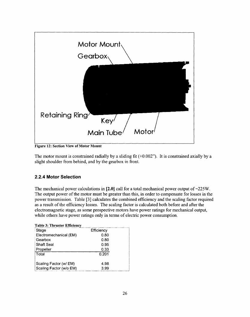
Figure 12: Section View of Motor Mount

The motor mount is constrained radially by a sliding fit (+0.002"). It is constrained axially by aslight shoulder from behind, and by the gearbox in front.

2.2.4 Motor Selection

The mechanical power calculations in [2.01 call for a total mechanical power output of -225W.The output power of the motor must be greater than this, in order to compensate for losses in thepower transmission. Table [3] calculates the combined efficiency and the scaling factor requiredas a result of the efficiency losses. The scaling factor is calculated both before and after theelectromagnetic stage, as some prospective motors have power ratings for mechanical output,while others have power ratings only in terms of electric power consumption.

Table 3: Thruster EfficiencyStage EfficiencyElectromechanical (EM) 0.80Gearbox 0.80t Shaft Seal 0.95Propeller 0.33Total 0.201

Scaling Factor (w/ EM) 4.98Scaling Factor (w/o EM) 3.99

26

Motor Mount

Gearbox\

,-,., I, , , Key/ /

Main Tube /

....... . ..................... ......... .... . ..... ...... . ..... .... . .... . ................. .......... ..... ................... ......... ........................... ............ ....... ..

D'ir

Motor

Within the power target and budget, a pair of drill motors was selected. They are rated at 300Wmechanical combined, running at 7.2V. The system will operate at 12V, allowing a maximumpower draw of 800W. Under these conditions for a sustained period, the motor will overheat andpotentially melt. A conservative assumption is made that the system will operate at a 50% dutycycle. This brings the motor to 400W output, 33% higher than nominal. In all likelihood themotors will operate closer to 20% duty cycle.

2.3 Pitch Actuator

The pitch actuator is the top of two stacked actuators controlling the thruster. Because the Yawactuator must move the pitch mechanism. This means that the pitch mechanism should not haveexcessive mass. The actuator also has parts that stick out of the hull into the water. This meansthat the upper structure should be as streamlined as possible, to reduce drag and added masseffects. The structure must still be stiff, however, as the entire thrust load from the thruster mustbe transferred through the actuator to the ROV.

2.3.1. Structure

In order to minimize the drag on the structure in flight, the thruster is mounted on top of twoslender spars. These put the thruster away from main hull, giving the thruster a greater range ofuseful outputs.

The structure is loaded under three conditions. First, the thruster applies a reaction force onto thestructure, inline with the thruster. Second, when the thruster is being rotated, the mass and addedmass effects apply a torque to the structure inline with the axis of rotation. Third, the assemblycontacts foreign objects, applying forces or torques.

Figure 13: Load Cases

Under the first loading condition, the force is transferred from the thruster to the spar bearings inthe radial direction. The spars then take the load in the long direction. Both of these are thestiffest cases. Normal thruster loading sees the stiffest structural response. Under the second

27

Mie--.II

Fcontact

Fthruster

v1

(1) (2 (3- r- fi /(1) (2) (3)

loading condition, the force is transferred from the thruster to the spar bearings, again, in the stiffradial direction. The spars each take the load in the stiff long direction. Each spar takes the loadin an opposite direction, though. An additional moment load is also experienced by the spars,however. The slender spars are relatively compliant in torsion. The third load case acts as alump condition for all remaining loads. Most notable of these cases is loading the thruster acrossthe spars. This transfers force axially through the bearings and to the thin dimension of the spar.This is the most compliant arrangement.

2.3.2. Drive System

The pitch actuator is driven by a timing belt and pulley system. This design allows the motor tobe located in the base of the structure, inside the hydrodynamic profile of the vehicle. The belt islocated inside one of a pair of slender spars. Only a small bearing, pulley, and pulley housingare required at the output shaft at the top of the spar.

28

Timing Belt Pulley

Figure 14: Section View of Pitch Actuator

The lower timing belt pulley shaft is constrained by a pair of radial bearings. The load is purelyradial, so no pre-tensioning of the bearing assembly is needed. The pulley is fixed to the shaft.One bearing is constrained between the pulley and the pulley shell. The pulley shell is adetachable cover which contains a bearing seat. That bearing is axially constrained between theseat and the pulley. It is radially constrained by a sliding fit (+0.002") on the outer race. Theother bearing is constrained between the motor mount and the pulley. As with the first bearing,the second bearing is constrained axially in one direction and radially by a sliding fit bearingseat. The other axial direction is constrained by the pulley. The pulley shell is fastened to themotor shell by four long 6-32 machine screws. The housing was blanked and machined as asingle piece, then cut and finished. This minimizes the problems from misalignment.

The upper timing belt pulley is attached to a shaft press fit into the thruster. One radial bearingin each blade constrains the thruster in the radial direction. Spacers are used to constrain theshaft in the axial direction between the fixed components.

29

Bearing

Blade Hub

Timing BE

Base\,

de (2x)

or Mount

\Mofor Shell

3earmotor

Pulley Shell/ \Timing belt Pulley

2.4 Yaw Actuator

The yaw actuator needs to be stiffer and stronger than the pitch actuator, because it is the bottomin a pair of stacked actuators. While the pitch actuator only needed to control the mass of thethruster, the yaw actuator must control the mass of both the pitch actuator and the thruster.Also, any angular deflection from the bearings or structure will cause a large deflection at thethruster end of the structure; this is a sine error.

2.4.1. Structure

The yaw structure is manufactured from a single block of acetal. This ensures that the gears areproperly spaced, and are not subject to variation from assembly and fastening. The housingblock is fastened to the pitch actuator by a set of countersunk machine screws. On the other side,the output shaft is mounted to the anhedral connector (more below) with a press fit.

Locknut

GearmotorN

Motor Mount-, (2x)

}ear

/

Seal

Bearing-

32 Tooth Gear

Motor ShcExtension

Figure 15: Section View of Yaw Mechanism

30

2.4.2. Drive System

The drive system is a simple spur gear reduction. Both the drive and driven gear are cantileveredout from the housing block. The output shaft is constrained in the radial and angular directionsby a pair of radial bearings. It is constrained axially in one direction by the 96 tooth gear pressfit (-0.002") on the shaft. In the other axial direction it is constrained by a locknut. The locknutallows for variable preloading in the axial direction. These ball bearings are not designed forheavy preload, so the applied preload is just enough to eliminate the backlash in the axialdirection. The bearings are constrained in the radial and angular directions by a sliding fit(+0.002") between the outer race and the housing. They are each constrained axially in onedirection by the counterbored surface of the housing. They are constrained in the other axialdirection by the shaft assembly.

The motor shaft extension is press fit (-0.002") directly onto the output shaft of the motor. Thisconstrains the shaft in the radial, axial, and angular directions. An additional bearing is mountedon the shaft extension in order to reduce the moment loading on the motor. This causes thedesign to be overconstrained. The additional room required to implement a flexible couplingwould make the assembly too large to comfortably fit in the system. In order to mitigate theoverconstraint, the motor mount is carefully machined, with additional allowances in the screwholes and in the bearing seat. This allows the structure to resist loads while having a degree ofcompliance to reduce the damage that any misalignment causes.

2.5 Body

The body connects the two thruster assemblies together. Under mission conditions, it wouldincorporate a selection of sensors and payloads. Instead, it contains dummy ballast andfloatation.

2.5.1 Anhedral Connector

Anhedral is the angle from horizontal down to the thruster mounts. This angle is used in order tooptimize the range of motion use, in conjunction with modifications to the control scheme.

31

Figure 16: Anhedral Connector: Hidden (grey) holes comprise the base scale in the yaw half. Visible (black)lines comprise the vernier holes in the fixed half.

The anhedral connector allows the selection of different anhedral angles for the thrusterassemblies. It uses a vernier type hole arrangement to allow angles from +90 to -90 in 7.5°

increments. The half connected to the yaw mechanism has holes drilled at 30° increments. Thestationary half has a pair of holes at +90°. This allows positioning at the base scale of 30°

increments. A second pair of holes is drilled at -45° and 135°. This allows positioning at thebase scale +15°. A final double pair of holes allows positioning at the base scale +7.5, or +7.5and +22.5°.

2.5.2 Ballast and Floatation

A bar extends from the main crosspiece vertically both up and down to mount the buoyancy andballast, respectively. The bar is manufactured from a 1" piece of sheet aluminum bent into a U-shaped cross-section. Lead weights are used for ballast. Syntactic foam is used as floatation.Syntactic foam is a special hard foam filled with glass bubbles. Although it also has applicationsin aerospace and rapid prototyping, most syntactic foam is designed as floatation for submarines,offshore rigs, and buoys.7]

This system passively maintains orientation in pitch and roll. In a neutral position, the ballastand flotation are inline with the center of mass and gravity. Any deviation in the pitch or rolldirections forces the floatation and ballast to move out of line with the center of mass andgravity. This creates two moment contributions: one from the ballast, and one from thefloatation. The two contributions sum to create a restoring moment, bringing the system back toa neutral state.

32

F_float

Momentj0~~ ~ ContrbuL

I Cmass

L F_oat

I

Fballast F_ballast

Figure 17: Ballast and Flotation Righting Moments

33

4

entrbutlon

..I... ."I .... . ... I.... - .. . I., .. - - I .. .. ... -.1 ... ... .... .." .. .I.I.I.- � ...I... ... .. .. ..... ......... . I.- .....I ......- ...I...... ....... � ..... 111- .... - .I... ...-, ....... .. .

Il

f

3.0 Control System Design

The control aspect can be divided into several basic parts. The first part is the servo controllerthat takes in command angles for each joint, and directs the motors. The second is the kinematiccontroller that converts high level direction input (move up, down, etc) into the necessary jointangle commands. Last is the user interface that converts human input into high level directioninput.

PC Terminal - --, PC Termnal m

I aCo11 U -o-i ~ Controller XCorol er

Figure 18: Control System Architecture

3.1 Mechanism Servo Control

The servo controller is the basic feedback loop for the motors, controlling output position. Theloop is a PID control loop. Initial estimates of parameters were calculated by geometry. Finalparameters were tuned in the operational environment.

Both of the positioning axes are controlled with DC gearmotors, and will have control models.Motor parameters are calculated based on the manufacturer's torque-speed curve (Fig. 19). The

34

IIIIIIIIIIII

III

II

II

II----- :

torque constant, Kt is equal to the back EMF constant, Ke in SI units, by conservation of energy.This is assumed true for all motors. A single constant, Ke is used in this analysis. Thisparameter is derived as the relation between voltage and speed.

V 6 0K----- 0.028 v =0.003 e 0 210 RPM radis

(1.15)

Figure 19: Torque-Speed Curve for Copal Gearmotor HGI6-030AA 'I

The motor is controlled using voltage, because this is easy to generate with PWM hardware. Thealternative, controlling with current, is significantly more difficult to implement in hardware.The motor acts as small feedback loop (Fig. 20). First, the back EMF is subtracted from theinput voltage. The back EMF, VEMF, is related to the output speed C through the motor constantKe.

VEMF = K Q (1.16)

The difference between the input voltage and the back EMF is the error signal in the feedbackloop, or the remaining voltage which will cause a change in the output of the system. This is fedthrough the equivalent resistance R and inductance L of the motor to create a current I.Calculation in the Laplace domain greatly simplifies the problem.

Imotor (S) = (VinPUt (S) -VEMF(S)) -mc ~~Ls±R

35

(1.17)

The torque output from the motor windings is related to the current through the windings againby the constant Ke.

Tmotor (S) = Iwindings (S) Ke (1.18)

Any disturbance torques, as from the load, are subtracted from this motor torque. Theremaining, or net torque, is applied to the mechanical system with an equivalent moment ofinertia J and viscous damping C. The output velocity is then

(1.19)Qnmotor (S) =- ( input (S) - Tdisturbance (S) CJS + C

The new output velocity feeds back to the initial voltage difference through the motor constantKe.

Figure 20: Voltage Controlled DC Motor Block Diagram 91

The voltage controlled DC motor is part of the larger servomechanism. The output velocity isreduced with a 1:3 gear reduction, symbolically 1 :N. The velocity is also integrated by thephysical system to position, the variable being controlled. For ease of operation, the gearreduction and integration are modeled as taking place on the motor shaft. A degree ofcompliance is assumed from the motor shaft to the output shaft. (Fig 16)

Figure 21: Output Compliance Model

36

)motor Ooutput

L I

The compliance is modeled as a spring between the position of the motor and the position of theoutput shaft. The torque on the output shaft is proportional to the difference in angular positionfor the two shafts.

Topu (S) Kshaft spring (moorshaft (S) - output _shai (s)) (1.20)

This torque is equally applied on the output and motor shafts. The torque applied on the motorshaft takes the form of the disturbance torque into the voltage controlled DC motor. Themagnitude is reduced by the gear ratio 1 :N. The torque applied on the output shaft acts on theoutput mechanical system, with equivalent moment of inertia J and viscous damping C. Thevelocity output is integrated once to yield the position of the output shaft.

eoutput (s) = Toutput,, (s) (1.21)J + )

Figure 22: Servomechanism Control System Block Diagram

For both the pitch and yaw mechanisms, it is desirable to develop approximations for the motorand shaft inertias, damping, and stiffness. Ke was found earlier. The inductance L and resistanceR for the motor can be directly measured with an LRC meter. The rear reduction ratio is fixedby design. The motor shaft inertia J is approximated as a L = 10cm R = 0.5cm steel (p =7.85g/cm3 ) shaft.

Jcylinder = MR2 (1.22)

shaft = (steel .tR2L)R 2

The damping is measured by recording the no-load torque required to spin the shaft. This is alow-accuracy term. The output shaft inertia is calculated in SolidWorks. The inertia of the yawdirection varies with the position of the thruster in the pitch direction. This is because the pitchdirection controls the distribution of thruster mass in relation to the yaw axis centerline.

37

Table 4: Approximated Servomechanism ParametersParameter Pitch Yaw

Ke [V s/rad] 0.003 0.003L J[Hl 0.005 0.005

R [ohm 6 6

N 13 3

Jmotor [kg m ] 9.36x10 9 9.36x10 -9

Cmnotor [Nms/rad] 1.Ox 101 1.Ox 10lO

Jshaft [kg m] 2x10 -3 1.9x10-3+( 2x10-3*0_pitch)Cshaft [Nms/rad] 0.3 0.1

Kshaft [N/ra 1 x 1X0 6 2.3x 10 6

With the entire physical system modeled, the reduced feedback loop for the system can bedeveloped. A potentiometer measures the position of the output shaft. A prefilter andcompensator are implemented to stabilize the system. The design of these components arecovered in the following section.

Figure 23: Reduced Feedback Loop

3.1.1 Compensator Design

The compensator is designed with the understanding that it will be implemented in software. Aset of discrete time approximations for PID control are implemented. The proportionalcontribution is a constant, and so it is the same as in the frequency domain. In software, this issimply the present error signal multiplied by a constant.

Vp (s) z vp(t) = Kp e(t) (1.23)

The differential contribution is the time derivative of the error signal, scaled by a constant. Insoftware this is approximated as the difference between the present value and the valueimmediately before, scaled by the length of time between the samples, and scaled again by theconstant.

38

-IV(s) Qou1

PhysicalSystem

........... ..............

-].. .................

I "P {

....... . AtThe integral contribution sums is the sum of all differential elements up to the present time. Insoftware, this is implemented as a sum of the error signals from the start of the command to thepresent time. More practically, the derivative error signal calculated for the differentialcontribution is added to a storage variable.

K (s) vi (t) = Ki E e(j) .At (1.25)j=0

3.2 Kinematic Controller

The kinematic controller is responsible for translating user commands into joint angles andthruster speeds. This is accomplished with a series of trigonometric and minimizationcalculations.

3.2.1 Analysis

In order to analyze the kinematics of the system, each joint is given its own coordinate system.Each is defined by a linear translation and rotation from the previous coordinate system. Thefour systems are, in order, the center of mass, base, yaw, and pitch. The center of mass system ismapped to the global coordinate system X-surge, Y-sway, Z-heave.

39

V, (S) -, V, (t = K,, -[e(t, - e(t,,-, A (1.24)

x

Figure 24: Coordinate Systems. Thin black axes represent a translation of the previous system. Thick axesrepresent current rotated system.

A series of homogeneous transform matrices (HTMs) are used to calculate the forwardkinematics of the robot. HTMs allow relatively easy conversion between coordinate systemswith both angular and linear offsets. Beginning with the dihedral (anhedral) angle of the thrustermounts at the base, the base coordinate system from the center (origin) coordinate system is

1 0 0 Xcenter to base

0 cos(V/) - sin(v/) Ycenter-to_base (1.26)

0 sin(q/) cos(y/) Zcenter_ tobase

0 0 1

Next, from the base to the yoke assembly coordinate system

cos(O) -sin(O) 0 Xbasetoyok e

sin(O) cos(O) 0 Ybase toyoke (1.27)

L°0 0 1 Zbase to yoke

0 0 0 1

From the yoke to the thruster coordinate system

40

centerbase

zI

'7

pitchX'

1 0 0 Xyoke to thruster

0 cos({) -sin(0) 1Yyoke to thruster (1.28)

0 sin() cos(¢) Zyoke to thruster

0 0 0 1

The three HTMs are combined symbolically into one large 4x4 homogeneous transform matrixwhich is the total change between the base and thruster coordinate systems.

cos (0) -sin(H).cos (m) sin(O)- sin(v)

cos(W).sin(0) cos()cos(o).cos(V) - sin(+).sin(v) -cos(W).cos(0)-sin(^) - sin(+).cos()

sin(+).sin(0) sin(+)-cos(O)-cos(w) + cos(4).sin(w) -sin(+)-cos(0)sin(v) + cos(W).cos()

0 0 0 ... (1.29)

cos(0) Xdih - sin(0).Ydih + 2 Xpan

cos(p).sin(0).Xdih + cos().cos(0).Ydih- sin(+).Zdih + cos(+).Ypan - sin(+).Zpan + Ytilt

sin(4).sin(0). Xdih + sin(+).cos(0).Ydih+ cos(+).Zdih + sin(+).Ypan + cos(+).Zpan + Ztilt

1 )

The thrust value for each thruster is calculated by dividing the initial XYZ input vector by itsmaximum possible magnitude. These HTMs allow conversion between XYZ coordinates and0,4 coordinates. The thrust calculation gives the output coordinates a full set of 0,q,Mcoordinates.

In the software implementation, a direct inverse kinematic approach is taken. This allows thetrig computation to be kept to a minimum, using only the arctangent during the function call.The first transform is used, although since the anhedral angle does not change throughout themission, the sine and cosine components are calculated at initialization.

AnhedralCOS = cos (W) (1.30)

AnhedralSIN = sin (,)

Then at each software call, only the multiplication is required. The matrix structure is removedfor calculation in ANSI C.

y ' y AnhedralCOS + z AnhedralSIN (1.31

z ' = z .AnhedralCOS + AnhedralSIN

The inverse kinematics consist of two arctangent operations. The first determines the angle 0.

0 =arctan lJ (1.32)VXI

41

The second determines the angle . This angle requires the magnitude of the vector in the XZplane.

0, =arctan( X12I+Z1 (1.33)Y.

The thruster magnitude is initially treated as the average magnitude

~M ~ =~Xi,~ +~yJ +Z, (1.34)3

If x ... z1 are given a maximum of 1, this method only allows maximum thrust with a fullcomponent in each direction. The maximum output for thrust purely in the x, y, or z direction is1/3. A more advanced possibility allows the thrusters to command the maximum output in anydirection. This would be implemented by comparing the average magnitude to the maximumpossible magnitude for a particular ration of x y and z. In software, a lookup table would beused.

In order to make the ROV usable by unskilled operators, a higher level of control must beimplemented. This level takes user commands (X,Y,Z,®) for the total robot and generates XYZ,then 0,q,M commands for each thruster. Because the system is over-actuated, there is not a one-to-one mapping of output translation to input commands. Several sets of thruster XYZcoordinates can produce the same ROV X,Y,Z, ) output. In order to be able to produce aprogram that is capable of selecting an appropriate set of coordinates, a set of values areminimized. First, the system seeks to use the minimum possible thrust. Second, the systemseeks to move as little as possible to the next position.

3.2.2 Low Level Algorithm

The simplest algorithm satisfies the thrust minimization, but does not satisfy the motionminimization. To satisfy force balance, the sum of each thruster contribution must add to thetotal desired output. To satisfy moment balance, the contributions must be equal for translation.To accomplish this, each thruster takes one-half of the input displacement command in X,Y, andZ. The 0 input is also split, but with one of the halves reversed in sign to create rotation.

X X Xi -- ~+ X2 ---2 2 2 2

Y YY =2 Y2=2 (1.35)

2 2Z ZzI- 2 Z2 = 2

42

Or in matrix form

I _ Ix

2 2 Y

0 0 = y,l\ o o

2

0

0

0

12

0

0 iL } 4X 20 0 = Y2

1 7 0 2

(1.36)

3.2.3 Advanced Algorithm

A second, more advanced algorithm takes advantage of running the thrusters in reverse toprovide more options for thruster positioning. The system identifies all possible configurationsthat satisfy the thrust minimization criterion. The closest one to the current configuration is thenselected. In this augmented version of the low level system, the second configuration takes thenegative of XYZ for both thrusters. An identifier bit is used to mark the coordinates as reversethrust. The distance from thestraight-line displacement.

current position to both possible configuration is calculated as a

XI~ _

y1 =0

ZI Forward

Yl _=

ZI Reverse

2 Y0 J7

002 0 )2

0 -0 0 -2 I 0

(1.37)

(1.38)

(1.39)A forward = (Xforward - Xcurrent ) + (Yforward - Ycurrent )2 + (Zforward - Zcurrent )

AI reverse = (Xrerse -se Xcurrent ) + (Yreverse -Ycurrent )+ ( Zreverse Zcurrent )

43

3.3 User Interface

The user interface is kept to the minimum required for operation. The interface sends basiccommands, such as forward and back, and receives a constant stream of system parameters. Thetopside control is a Visual Basic application using the MSCOMM serial protocol.

Figure 25: Visual Basic Control

Initial testing is done with a joystick plugged directly into the controller hardware.

3.4 Controller Hardware

The onboard hardware consists of a custom embedded microcontroller system. The controllerwas previously designed by the author as a leg controlling slave board for an amphibiouswalking robot. The board has onboard capability for four motors drawing up to 5A each, 32analog inputs, and two channels of asynchronous serial (RS-232 compatible). A commercialmotor driver is used to operate each of the main thrusters.

44

Table 5: Control Hardware Requirements and ImplementationArea System RequirementSmall Motor Driver 4 - 12V, 2A motors (Pitch and yaw for

two assemblies)Large motor Driver 2 12V 15A (two main thrusters)

Sensor input 4 analog in (position potentiometers)10 analog in (accelerometers/gyros)4 sensors (depth, ??????)

Communications RS-232 Uplink to PC

Computation 500 Hz? Processing and servoing

Hardware Specification/implementation4, 5A each, 24V max

Commercial RC Motor controller 36V 24A- driven by 2 digital /O pins on board32 multiplexed analog inputs to 10 bit A/Dconverter

Hardware UART with RS-232 level shifter,up to 115200 bits per second.10 MIPS (million instructions per second)for average cycle time of ?? s = ?? Hz

The controller uses a Microchip PIC 1 8F458 programmed in mixed C and assembly as a generalpurpose microcontroller. Small motors are driven by the next generation Motorola M33887 H-bridge IC. The M33887 has ultra-low on-resistance and fast switching times to minimize theenergy dissipated as heat. This allows control of motors at 5A in a 1" x 0.5" x 0.1" (LxWxH)package with only ground plane heat sinking. This allows a tighter board design than traditionalH-bridges would allow.

figure Lo: Control System iVain soard

For testing, the control system was kept out of the water. This means that the tether carries all 12motor wires plus a minimum of 6 sensor wires. In a practical implementation, the tether wouldonly carry power and a bi-directional data line, in order to minimize the cost and stiffness of thetether; if the tether is too stiff, the motion of the ROV may be severely impaired. Creating awaterproof control housing is a well defined and solved problem; it was not repeated in thisresearch in an effort to reduce the system complexity and potential modes of failure.

45

4.0 Experimental Validation

The experimental portion takes two major forms. First, the ability of the mechanism to moveinto position on command is measured. This includes positioning accuracy including backlashand compliance, and speed/bandwidth. Second, two of the devices are mounted on a hull, andthe ability to control motion in all six degrees of freedom is measured. Although only fourdegrees of freedom have user inputs, the remaining two, pitch and roll may be activelyconstrained by the control system, and so are also relevant outputs. The positioning/velocitycapability of the system is again measured in terms of accuracy and bandwidth.

4.1.0 Single Mechanism: Setup and Procedure

The purpose of the single mechanism test is to measure the performance of the servomechanism,separate from any high level control system.

All joints except the active joint are commanded to hold a center position. The active joint issent a square wave command. The initial frequency is slow enough to allow a full step responseon both the rise and fall of the input signal. During the test, the frequency is increased until thesystem is unable to respond in any sort of coherent manner. Input and output waveforms arerecorded throughout the procedure. For each input frequency, the average final position iscalculated. The average final position is plotted against the input frequency to give the closedloop system response. The closed loop transfer function is also approximated from the graph.

The initial setup and test is done in the air, to allow for easy calibration and repair. The robot ismounted upright on a test stand.

Figure 27: Robot mounted on test stand

The second setup is designed to measure the system response while immersed in water. Therobot is mounted on its side, with one thruster assembly submerged. By arranging it in this

46

manner, only one electronic component is submerged: the pitch potentiometer. Although allcomponents have been sealed or otherwise waterproofed, this setup minimizes the potentialdamage to the system. This also is a better model for a full implementation of the system, wheremost of the mechanism would be within a plastic shell.

Figure 28: Servomechansim test setup for water

4.1.1 Single Mechanism: Results

The system response is measured for input frequencies ranging from 0.5Hz to 9 Hz, for a angulardisplacement of 130° for pitch and the and 170° for the yaw, representing a typical motion. Lowfrequency responses saw a clean matching of input command (Fig.29). High frequencyresponses showed a significant drop in magnitude, as the actuator was unable to keep up with thecommands (Fig.30). Relatively high overshoot on the yaw is a result of the predominantlyproportional tuning of the PID loop.

47

-

Position Response (Counter = 30 cycles)

- ,.

200

CUa

" 150M._

SC 1000r.2

:.IUn0

50

00 O C) ') C0 o C NI I- .O - ) 0 ) 0O) ' COo O o - O- ci Ci N o CC: C O (Co r - r- -

Time (seconds)

Figure 29: Low frequency input and system response. 30 cycles - 0.3 Hz

Position Response (Counter = 6 cycles)

ZOU

200U)C-

L 150I,

C

c 100

.200

50

0

0.0 0.5 1.0 1.5 2.0 2.50.0 0.5 1.0 1.5 2.0 2.5

Time (seconds)

48

- Pitch ]

-i- Pitch Command -- Yaw

Yaw Command;

Figure 30: High frequency input and associated magnitude decrease. 6 cycles 2Hz

ZOU

This data was recorded for 13 different frequencies. The relative magnitude is compared to theinitial command magnitude in a frequency response plot (Figs.31,32)

System Response - In Air

10

.'

00mO19

aEe"O}

1

0.1

Frequency (rad/s)

Figure 31: System Response in Air

The frequency response shows a bandwidth of approximately 6 rad/s or -1 Hz for the pitchactuator, and approximately 10 rad/s or -2 Hz for the yaw. After these frequencies theperformance degrades along a two decade per decade line. The system closed loop transferfunction can be modeled in its simplest form as

Tpitch (s)=(6+ s)p ch! (6 + S)2 (1.40)

(1.41)1

Yaw(S)- =(10+ s) 2

49

:i-7-

\

[ - - i -- -- --

I - -- J- -

System Response - In Water

10

0

0)aU

0.1

0

Frequency (rad/s)

Figure 32: System Response in Water

As before the transfer functions can be approximated.

1Tpitch (s) =(I(6 + s)- - - - -

-, , I

(1.42)

T (s) = (1.43)yaw (Io + s) 2

The waster test was conducted at a higher input voltage, resulting in approximately equalresponses for air and water. Both air and water tests were conducted at a voltage just below thevoltage at which the system would go unstable. Although the pitch axis has less inertia than theyaw axis, the belt drive mechanism of the pitch actuator has significantly more damping than thegear train on the yaw actuator. This explains the faster response of the yaw actuator.

4.2.0 ROV Mount: Setup and Procedure

The purpose of the ROV mount test is to quantify the performance of an ROV using the novelthruster technology. This performance is the primary motivation for the research. As with thesingle mechanism test, the accuracy and speed of output position are measured.

The challenge with this procedure is to measure and decouple motion in all six directions. As anexample, for surge or forward motion, both the forward speed and the parasitic motion in the

50

- J = - .Rtoh _ , -__ -s --Yaw -< _ _ -- _ a= ==- ==. , .- ~t--- X I

' i:Xf \ X:X-0>:.- .-, e - --- -----_-~ ' '' 1

~~~~_ _ _ _ _ _ _ I __ _ _ _ __ _ _ _

1

other directions are relevant. The preferred setup is to use a six-axis measurement system, eitheran inertial measurement unit (3 accelerometers and 3 gyroscopes) or a camera setup. This allowsall six directions of interest to be measured simultaneously for any input.

An alternative setup uses a battery of single axis measurements to record the most interestingaspects of the response, or all aspects over a much longer series. Measurement technologiesinclude using string pots, depth sensors, and single axis accelerometers or gyroscopes.

4.2.2 ROV Mount: Results

Failures in the mechanism and control system prevented successful free-swimming tests.Additional tests will be carried out in future work with replacement hardware.

51

5.0 Analysis / Discussion

Table 6: ROV Performance v. Initial SpecsParameter Initial Specification Prototype Spec Commercial BenchmarkMass 5kg 3kg 3kgSize 0.35m sided cube 0.6x0.2x0.3m 0.35x0.25x0.21mMax Speed 5mn/s -- 2.5m/sMax Acceleration 1 to -m/s in 1 second -- --

Although a full system, free-swimming test was not performed, it is possible to judge thepotential performance of the system of the servomechanism test. The mass specification wasmet. The size specification is met in volume (V=0.035m 3 , Vspec=0.043m 3 ), although the longestdimension is larger than both the commercial and initial specification.

The max speed has no quantifiable data on it, although the power output analysis suggests thatthe current system is capable. In 2.0.1, the power lost through drag was estimated as -6W,rounded up to l OW. The 400W combined mechanical output of the motors can suffer a 40X lossin transmission while still meeting the specification. The estimated loss in transmission wascalculated as 4X, although this was for the optimum configuration. Certain thrusterarrangements will have a significant obstruction to the water flow, reducing efficiency. Thesystem is still overpowered for the drag spec, although this was identified as not a limitingcriterion.

The largest contributor to power loss, and last specification is acceleration. The initialspecification called for acceleration from lm/s to -lm/s in 1 second. By reversing the thrusters,this can be achieved without the servomechanism. Although the motor power output ismarginally capable of this spec, the additional 2kg remaining on the mass requirement can beused for larger motors. However, most propellers have a drastically reduced performance inreverse. A better method may be to use a highly efficient propeller in one direction, whilerapidly positioning the thruster. In order to meet this requirement, the thruster must, as aminimum, be able to position within the one second. This would leave no time for thruster towork. Ideally, the positioning would take as little time as possible, in order to allow themaximum time for thruster output. With the current servomechanism, the fastest response beforesignificant degradation is approximately 2Hz. Although the pitch actuator is only 1 Hz capable,it operates over half of the range.

With a 2Hz output, half a second is available for thruster output, under worst-case conditions.Because the same energy is required to change the velocities, the power to do it in half the timewill be twice as much. This will require larger motors or a relaxation in the initial specification.The current system would be capable of decelerating from m/s to - m/s in 1.5 seconds.

If motors with twice the power output were used, the additional mass would slow the systemresponse down, and so would require additional time for positioning. More powerful thrusters ofan equal mass and size would prevent this problem. Because relatively coarse, low efficiencymotors were used in the current design, this is a non-trivial solution. Identified alternatives

52

include high power density model airplane motors from Astroflight, Inc. Assuming for now thatthis is not possible, An additional lkg of available system mass will be distributed to thethrusters, 0.5 kg to each. This doubles the current 0.5 kg each. The addition of this mass willincrease the pitch moment if inertia by 1.9x, and the yaw moment by 1.5x (accounting foradditional mass of structure and drive train). The additional inertia will degrade the positioningperformance, although not severely. In examining the experimental results in section 4, it isapparent that the limiting factor in positioning is the steady-state output of the motor. Theacceleration and stabilizing periods account for only one fourth of the total motion. Furthermore,a proper retuning of the PID loop should be able to reduce this significantly. Even without afaster stabilization, however, the additional inertia will only increase the acceleration portion ofthe motion. With a conservative twofold increase in acceleration times, the new total positioningtimes will be

te, = 0.5 .(0.75 + Iactor 0.25)

tnewmax = 0.5.(1.25)=0.625s (1.44)

The thrusters will thus have to be only -2.5X the current output. In summary, the existingservomechanism is capable of meeting the performance specifications with moderately morepowerful thrusters.

53

6.0 Conclusion

In this research, a highly maneuverable ROV is designed and manufactured. The intent is tocreate a platform that is useful as a small inspection-class robot. In addition, the research aims tocreate a design than can be scaled up to larger work-class ROVs. A set of industry-leadingspecifications was chosen as a design target.

In the first design section, system parameters were examined to determine the relevance of eachon the system performance. Thruster power was identified as the primary performance driver.Momentum effects, or acceleration, were identified as the primary draw of this thruster power.In the second section, a variety of possible propulsion arrangements are considered, bothtraditional and novel. The four designs of most interest include arrangements with: four fixedthrusters; two thrusters with two degrees of freedom each; a surface covered with small jets; anda combination of surface jets and thrusters. The two thruster design was selected because itcould provide full power in all direction, and relied on existing technology. In the next section,the detailed mechanical design of the robot and any associated analysis was carried out. In thesecond design chapter, the control system was designed. A low-level PID controller wasimplemented in software. A high-level kinematic controller was also created, in order togenerate joint output angles from high-level input commands, such as move forward, turn, etc.After this, the next section describes the experimental results from testing. Lastly, the results areanalyzed in terms of the initial specifications. Although a full-system test was not performed,the servomechanisms are capable of performing well enough to meet the specification.

Although the closed-loop servo tests proved to be successful, no conclusive data was generatedin testing the entire system. A combination of mechanical and control failure contributed to this.The obvious and immediate future work is in constructing a second-generation mechanicalassembly, suitable for long-duration testing and operational conditions. In addition the controlsystem should be revised to minimize the system resources used on algebraic and trigonometricoperations. Trig look-up tables and clever manipulation of variable types will accomplish this.Additional future research includes finding the optimum anhedral angle, and modifying thecontrol system to take advantage of this. Also, a full-body faring should be implemented tominimize drag during free swim tests. Overall, the design appears very promising, and warrantsthis future work.

54

Appendix A: Control System Schematics

|Reset

JICD2

JICD C

CN6

d- I

"- 2

- 3- 4-5

J5

Fa I

1-- 2

R 41 4

10k7

Daniel Walker Reu 1.1Daniel W5a05/205 Page I of 3

55

3

CL

._0

3

0'2

I r-

3

C

L

a

£

0

U)R

ub

us0E

II-- 1- -i City I -_V -1 A 'k- a4

t $a,

ID

3IClAI

0rM -19-4

co

'o

ru

a)

00

C)03

0s-h

(DID

-iID

;00C

56

rn'WI[<I

-

I

ttf

rID:EU

(D 'L4 C

asCD

'D

o

C)

(0

00

C)0:3Cl

0

(D

N-)

57

-i

I

-:3-LAlI

0-C

--

------

I

I

I

Appendix B: Control System Code

Thesis.C - Main Program Loop

//II Thesis Robot Controller//

I/ Daniel Walker 2003 - 2005

#ZERO_RAM

#include <18F458a.h>#include <18F458defs.h>

#include <slavedefs.h>#include <interrupts.h>

long int counter,counter2;#define pathlength 4unsigned int ComArray[4][pathlength] = {200,70,70,200

200,70,70,200,30,30,200,200,30,30,200,200};

//lpitch//ryaw//lyaw

void main(void)

/InitializeSlave(;QuickCalcs();

while (True)

'for (counter2=0;counter2<pathlength;counter2++)/RpitchCom = ComArray[0][counter2];LIpitchCom = ComArray[ ] [counter2];RyawCom = ComArray[2][counter2];LyawCom = ComArray[3][counter2];counter = 15;

ReadJoysticks();CalcAngles(Xcom,Ycom,Zcom,Qcom,0.0);

ThrusterDutyl = 133;

ThrusterDuty0 = 75;

while(counter-->l)

{

ReadAllAnalog(;

Lpitch = Lpitch+Lpitchzero;Lyaw = Lyaw+Lyawzero;Ryaw = Ryaw+Ryawzero;Rpitch = Rpitch+Rpitchzero;

58

//rpitch

I-I-/IH/

I-

fprintf(COM_A,"%5.2f,%5.2f,%5.2f,%5.2f, \n\r",Xcom,Ycom,Zcom,Qcom);

DoFeedback(O, CalcFeedback(0,Rpitch,RpitchCom));DoFeedback(1, CalcFeedback(1 ,Lyaw,LyawCom));DoFeedback(2, CalcFeedback(2,Ryaw,RyawCom));DoFeedback(3, CalcFeedback(3,Lpitch,LpitchCom));

fprintf(COM_A,"%3u,%3u, %3u,%3u, %3u,%3u, %3u,%3u, \n\r",Rpitch,RpitchCom,//fprintf(COMA,"%3u,%3u,%3u,%3u\n\r",PWMduty[0],PWMduty[1 ],PWMduty[2],PWMduty[3]);

}~~~~~~~~

59

Slavedefs.h - initializes and defines main functions

#fuhses HS,NOWDT,NOPROTECT,NOLVP#use delay(clock=40000000)

#use rs232(baud=1 15200, xmit=PIN_C6, rcv=PIN_C7, STREAM=COMA)#use rs232(baud=38400, xmit=PIN_C4, rcv=PIN_C3,STREAM=COMB)

#include <slavemath.h>

//10 pins

#define ActiveLED

#define#define#define#define

#define#define#define#define

#define#define#define#define

EN0ENIEN2EN3

PORTE,2

PORTB,0PORTB, 1PORTB,2PORTB,3

PWM0PWM 1PWM2PWM3

PORTD,1PORTD,3PORTD,5PORTD,7

DIR0DIR1

DIR2DIR3

#define ThrusterO#define Thrusterl

//Analog Portsunsigned intunsigned nt

#define#define#define#define

#define#define#define#define

PORTD,0PORTD,2PORTD,4PORTD,6

PORTC,3PORTC,5

joint,ADpin,ADmuxChan;ADres[4][8];

FaultStatus0FaultStatuslFaultStatus2FaultStatus3

FeedbackTempOFeedbackTemp 1FeedbackTemp2FeedbackTemp3

ADres[0][5]ADres[1][5]ADres[2][5]ADres[3][5]

ADres[0][7]ADres[1][7]ADres[2][7]ADres[3][7]

FeedbackCurrent0FeedbackCurrentlFeedbackCurrent2FeedbackCurrent3

RpitchRyawLyaw

ADres[0][7]ADres[1][7]ADres[2][7]ADres[3][7]

ADres[3][1]ADres[3][2]ADres[3][4]

60

#define#define#define#define

#define#define#define

#define Lpitch

RFRLthetaLLRRtheta

ADres[1][1]ADres[1][2]ADres[1][4]ADres[1 ][6]

Z_inY_inQ_inX_in

ADres[1][1]ADres[1][2]ADres[1][4]ADres[1][6]

Lpitchzero=235,Lyawzero=253,Ryawzero=0,Rpitchzero=1 0;LpitchCom=1 27,LyawCom=1 27,RyawCom=1 27,RpitchCom=1 27;ThrusterCount,ThrusterDuty0= 03,ThrusterDuty 1 = 150,ThrusterPeriod=4000;ThrusterFW = 129,ThrusterRV = 75, ThrusterMID = 105, ThrusterRange=28;

//PWM commandsunsigned int PWMcount,PWMperiod=31,PWMduty[4];

//#defineTimerOffset#define TimerOffsetPWM set for this value!//#defineTimerOffset//#define TimerOffset260

unsigned inmtunsigned intunsigned intunsigned inmtfloat

0x0D0OxOAO

0x04A0

0x041OxOOO

//2kHz PWM, 203 cycles with overhead 730//lkHz PWM, 396 cycles with overhead 550 !thruster

//500 Hz PWM, 775 cycles with overhead 260//500 Hz PWM, 775 cycles with overhead

CommSTAT;i;temp;count;

temp2;

//unsigned int jointpos[4],jointcom[4]={ 127,127,127,127 };float err[4],errlast[4];float Kp[4]={ .5,0.1,0.1,0.15 },Kd[4]={0.02,0.01,0.01,0.02 } ,Ki[4] = {0.005,0.002,0.002,0.005 };

//rpitch, yaw, ryaw, pitch

floatfloatunsigned inmtfloatfloatfloat

Vout[4], Voutmax=12.0;)D_contribution,P_contributionI_contribution,delta_t=0.016,Integratorsum[4];

I_LastCom[4];AnhedralCOS,AnhedralSIN,AnhedralAngle = 0.0;clistR 1,distR2,distL 1,distL2;Xcom,Ycom,Zcom,Qcom;

unsigned int MotorDISABLE = Obl I I I I 1,MotorTempWaming = 20,MotorTempLimit = 25,MotorTempWarningQC=0, MotorTempLimitQC;

I/Functions1111111111111111111111111111111111111111111111111111//Functions

61

#define#define#define#define

#define#define#define#define

unsigned intunsigned ntlong intunsigned int

ADres[3][6]

/---------------------------------------------------------------.//

/1 delay routine - leave as first. subsequent calls/ / ...................................... .........../ /

void Delay(float cycles)

{while(cycles>O)

cycles = cycles-1;

}

III

// ............................... //// Initialization

…// .. .......................... //

void InitializeSlave(void)

{set_trisa(ObOO101111);set_trisb(ObOO000000);settrisc(ObOO000000);set_trisd(ObOO000000);set_trise(ObOOOOOOOO);

setupadcports( A_ANALOG);setupadc( ADCCLOCK_INTERNAL);

//portb output//portc 3, 5 out for thruster pwm//portd output

//porta is all analog

fprintf(COMA,"\n\r\n\r\n\r\n\r\n\r\n\rLink Active\n\r"');I printf("\n\r\n\r\n\r\n\r\n\r\n\rLink Active\n\r");

enableinterrupts(INT_TIMERO);enableinterrupts(GLOBAL);

#asmbcf ENObcf EN 1bcf EN2bcf EN3

#endasm

//enable timer interruptI/set Global Enable

//clear to enable motor outputs

#asmclrwdtbcfbcfbsf

TOCON,TOPS2TOCON,TOPS ITOCON,TOPSO //write OxOO1 to prescaler

bsfbcf

TOCON,PSATOCON,5

clrf TMROL

//enable prescaler// select main clock source

I/start timer

62

11

#endasm

#asmlbsf

#endasmDelay( 10000);#asmbcf#endasmDelay(2000);#asmhsf#endasmDelay(2000);#asmbcf#endasmDelay(2000);#asmbsf#endasm

ActiveLED

ActiveLED

ActiveLED

ActiveLED

ActiveLED

/ .. ..... //1I read all analog inputs// . .............................. //

voidc ReadAllAnalog(void)

{for(ADpin = 0; ADpin <=3; ADpin++)for(ADmuxChan = 0; ADmuxChan<=7;ADmuxChan++)

#asmmovlw ObllllOO 1111000andwf PORTC,f

movfandlwiorwf

ADmuxChan,wObO0000111PORTC,f

//index ADinputs//index ADpin

//select MUX channel on ADmux//clear select bits

//kill top bits on ADpin//write bottom 3 bits

#endasm

set_adc_channel( ADpin );delayus(10);temp = ReadADC(;ADres[ADpin][ADmuxChan] = temp;delayus(l 00);

}

t/ ................................... ////send all AD values on UART

63

-----------------------------I/--- -----------------------------------I-

void TXAllAnalog(void)

{// fprintf(COMA,"\n\r");

for(ADpin = 0; ADpin <=3; ADpin++)for(ADmuxChan = 0; ADmuxChan<=7;ADmuxChan++)

fprintf(COMA,"ADpin %3u MuxChan %3u =%3u\n\r",ADpin,ADmuxChan,ADres[ADpin][ADmuxChan]);

//printf("ADpin %3u MuxChan %3u =%3u\n\r",ADpin,ADmuxChan,ADres[ADpin][ADmuxChan]);

//index ADpin//index MuxChan

III

II Quick Calcs: setup limit values// ...................................//voidc QuickCalcs(void)

{//Temperature Thresholds

I/ADout == 25.85*eA{ -.0405*[2550/(Temperature+10)] }float const Templndex[17] =

{ 119.27,132.17,144.97,157.42,169.29,180.41,190.63,199.88,208.13,215.38,221.70,227.14,231.78,235.78,239.03,241.8,244.12};

float const TempTail[16] ={ 12..9,12.8,12.45,11.87,11.12,10.22,9.25,8.25,7.25,6.32,5.44,4.64,4,3.25,2.77,2.32};

float QCindex=0,QCremainder=1/*,QCtemp*/;QCremainder = modf((((float)MotorTempWaming-20)/5),&QCindex);MotorTempWamingQC = Templndex[QCindex]+QCremainder*TempTail[QCindex];

QCremainder = modf((((float)MotorTempLimit-20)/5),&QCindex);MotorTemrnpLimitQC = TempIndex[QCindex]+QCremainder*TempTail[QCindex];

AnhedralSIN = SIN(AnhedralAngle);AnhedralCOS = COS(AnhedralAngle);

}

//…II . ////calculate feedback//err,temp: local// -- .-. - - - - - - - -- - - - - - - - - - - - - - - - - - - - - //float CalcFeedback(unsigned int joint, unsigned intjointpos, unsigned intjointcom)

{float Derror;

err[joint] = (float)jointcom-jointpos;D_error = ( err[joint]-errlast[joint] )/deltat;

64

fprintf(COMA,"%3u, %5.2f\n\r",joint, Derror);

Integratorsum[joint] = Derror+Integratorsumj oint];if (jointcom != I_LastComjoint])

it

I ntegratorsumljoint] = D_error;11 ~fprintf(COM_A,"%3u,%3u,%3u \n\r",joint, jointcom, I_LastCom[joint]);

D_contribution = Kd[joint] * D_error;P_contribution Kp[joint] * (err[joint]);I_contribution = Kijoint] * Integratorsumjoint];

Vout[joint] =Pcontribution + D_contribution + I_contribution;

errlast[joint]=errljoint];I_LastComr[joint] =jointcom;//saturation criterion

if (VoutUjoint] > Voutmax)Vout[joint] = Voutmax;

if (Vout[joint] <-Voutmax)Vout[joint] = -Voutmax;

return Vout[joint];

}

// ............................... //implement motor actuation

11//

void DoFeedback(unsigned int joint,float Vout)

{if (Vout>=0.0) //positive

{PWMduty[joint] = PWMperiod*Vout/Voutmax;

switch(joint)

{case 0:

#asmbcf DIR0#endasmbreak;

case 1:

#asmbcf DIR1#endasmbreak;

case 2:

65

#asmbcf#endasmbreak;

case 3:

#asmbcf#endasmbreak;} //end switch

DIR2

DIR3

} //end if positive

if (Vout <0.0) //negative --> pwm is now reversed

{PWMduty[joint] = PWMperiod*(1.O+Vout/Voutmax);

switch(joint)

{case 0:

#asmbsf#endasmbreak;

case 1:

#asmbsf#endasmbreak;

case 2:

#asmbsf#endasmbreak;

case 3:

#asmbsf#endasmbreak;} end switch

DIRO

DIRI

DIR2

DIR3

} / end if negative

PWMduty[joint] = PWMperiod-PWMdutyjoint];

//-I ..... /// ensure all otuput coordinates are within specified limits

66

II

#define LpitchMin 50#define LpitchMax 200#define RpitchMin 50#define RpitchMax 200

#define RyawMin 30#define RyawMax 220#define LyawMin 30#define LyawMax 220

void InsideLimits(void)

{if (LpitchCom < LpitchMin) LpitchCom = LpitchMin;if (LpitchCom > LpitchMax) LpitchCom = LpitchMax;

if (RpitchCom < RpitchMin) RpitchCom = RpitchMin;if (RpitchCom > RpitchMax) RpitchCom = RpitchMax;

if (LyawCom < LyawMin) LyawCom = LyawMin;if (LyawCom > LyawMax) LyawCom = LyawMax;

if (RyawCom < RyawMin) RyawCom = RyawMin;if (RyawCom > RyawMax) RyawCom = RyawMax;

III

/ / ... .................................../ /1I calc joint angles1-

//

void CalcAngles(float X,float Y, float Z, float Q, float anhedral)

float xl ,x2,yl ,y2,zl,z2,fl [2],f2[2],tl [2],t2[2],Nl1 [2],N2[2];

//initial minimization of thrustxl = X/2 + Q/2;x2 = X/2 - Q/2;

yl = Y/2;y2 = Y/2;

zl = Z_/2;z2 = Z_/2;

// modify output to match anhedral coordinate systemyl = yl *AnhedralCOS+zl *AnhedralSIN;y2 = y2*AnhedralCOS+z2*AnhedralSIN;

zl = zl *AnhedralCOS+yl *AnhedralSIN;

67

z2 = z2*AnhedralCOS+y2*AnhedralSIN;

// begin inverse kinematics (forward thrust)tl [0] = atan2(zl ,x1)*40+127;t2[0] = atan2(z2,x2)*40+127;

fl[0] = atan2(yl,sqrt( xl*xl + zl*zl ) )*40+127;f2[0] = atan2( y2, sqrt( x2*x2 + z2*z2 ) )*40+127;

NI[0] = (xl+yl+zl)/1.5;N2[0] = (x2+y2+z2)/1.5;

I repeat inverse kinematics (reverse thrust)tl[l ] = atan2(-z 1,-x 1 )*40+127;t2[1] = atan2(-z2,-x2)*40+127;fl [1] =-fl [0];f2[1] = -f[0];

N1 [1] =-NI[0];N2[1] = -N2[0];

I determine closest arrangemnt for thruster 1

distLI = abs(Lpitch-fl [0]) + abs(Lyaw-tl [0]);distL2 = abs(Lpitch-fl[1 ]) + abs(Lyaw-tl[1 ]);distRI = abs(Rpitch-f2[0]) + abs(Ryaw-t2[0]);distR2 = abs(Rpitch-f2[1]) + abs(Ryaw-t2[1]);

if ( (distL 1I) < (distL2)){LpitchCom = fl [0]; //convert from radians to 127 centered binary radiansLyawCom = tl [0];ThrusterDutyO = N 1 [0]*ThrusterRange+ThrusterMID;

// fprintf(COM_A,"1:0 %3u,%3u,%3u ",(unsigned int)LpitchCom,(unsignedint)LyawCom,(unsigned int)ThrusterDutyO);

}else

{LpitchCom = fl [1];LyawCom = tl [1];ThrusterDuty0 = N [ ]*ThrusterRange+ThrusterMID;

.11 / fprintf(COM_A,"1: 1 %3u,%3u,%3u ",(unsigned int)LpitchCom,(unsignedint)LyawCom,(unsigned int)ThrusterDuty0);

}

I determine closest arrangement for thruster 2if ( (distR ) < (distR2))

{RpitchCom = f2[0];RyawCom = t2[0];ThrusterDuty 1 = N2[0]*ThrusterRange+ThrusterMID;

68

// fprintf(COM_A,"2:0 %3u,%3u,%3u \n\r",(unsigned int)RpitchCom,(unsignedint)RyawCom,(unsigned int)ThrusterDuty 1);

else

RpitchCom = f211 ];

RyawCom = t2[1];ThrusterDuty 1 = N2[1 ]*ThrusterRange+ThrusterMID;

II fprintf(COM_A,"2:1 %3u,%3u,%3u \n\r",(unsigned int)RpitchCom,(unsignedint)RyawCom,(unsigned int)ThrusterDutyl);

InsideLimits(;

fiprintf(COM_A,"%3.0f,%3.0f,%3.0f,%3.0f\n\r",(float)distL 1, (float)distL2,(float)distRl ,(float)distR2);

III

/ / . ... ............................/ /II read the joysticks, convert to commands/1// -...........................................................//

void ReadJoysticks(void)

{ReadAllAnalog(;Xcom = (Xin-127.0)/127.0;Ycom = (Yin-127.0)/127.0;Zcom = (Zin-127.0)/127.0;Qcom = (Q_in- 127.0)/127.0;

69

Interrupts.h - handles PWM generation

#priority ssp,timerO// . ............................ //I PWM-TimerO interrupt routine// ,-//#[NT_TIMER0void timerie(voicld)

#asm#asmbcfmovlwmovwf

movfsubwfbtfssgoto

bcfbcfbcfbcfclrf

INTCON, TOIFTimerOffsetTMROL

PWMcount,wPWMperiod,wSTATUS,Ztest

PWM0PWM1PWM2PWM3

PWMcount

//reset overflow flag//reset timer with offset

//PWMcount /= PWMperiod?

I/turn all off, reset count

test: movf PWMcount,wsubwf PWMduty[O],wbtfsc STATUS,Z

bsf PWM0//PWMcount = PWMdutyO?

//turn on 0

movfsubwfbtfsc

movfsubwfbtfsc

mrnovfsubwfbtfsc

PWMcount,wPWMduty[1 ],wSTATUS,Zbsf

PWMcount,wPWMduty[2],wSTATUS,Zbsf

PWMcount,wPWMduty[3],wSTATUS,Zbsf

PWM1

PWM2

PWM3

//PWMcount = PWMdutyl?//turn on 1

//PWMcount = PWMduty2?//turn on 2

//PWMcount = PWMduty3?//turn on 3

incf PWMcount,f

mrnovf MotorDisable,wandwf PORTB,f

#endasm

if (ThrusterCount>ThrusterPeriod)

70

ThrusterCount=-O;#asmbsf ThrusterObsf Thrusterl#endasm

if (ThrusterCount==ThrusterDutyO){'#asm bcf ThrusterO #endasm}

if (ThrusterCount==ThrusterDuty1 ){ #asm bcf Thruster #endasm}

ThrusterCount++;return;

}

71

Works Cited

[l] Product Literature at http://www.videoray.com/Products/specs.php[2] Product Literature "LBV Standard System Specifications"

http://www.cetrax.com/detailed%201bv%20system%20descriptiondec%202002.pdf[3] National Research Council of the National Acadamies. Future Needs in Deep SubmergenceScience. Washington, DC. 2004.[4] Smits, Alexander. A Physical Introduction to Fluid Mechanics. p314.[5] Smits, Alexander. A Physical Introduction to Fluid Mechanics. p 31 8.[6] Techet, A.H. Reading #6 from 13.012 Hydrodynamicsfor Ocean Engineers. plO[7 1 Erikson, Ray. Mechanical Engineering. "Foams on the Cutting Edge". Jan 1999.[8 ] Product Literature "Copal 16mm Gear Motor HG 16 Series 60:1 Ratio"

http://www.copal-usa.com/PDFs/HG 16-060.PDF[9] Palm, William J. Modeling, Analysis, and Control of Dynamic Systems. p.185

72