L-H'ilOÜSlZ,

® 2

T Paul Scherrer Institut

Labor für Thermohydraulik

On Boundary Layer Modelling Using the ASTEC Code

B.L.Smith

Paul Scherrer Institut Telefon 056/99 2111 Würenlingen und Villigen Telex 82 7414 psi ch CH-5232 Villigen PSI Telefax 056/982327 PSI CH

PSI - Bericht Nr. 101

On Boundary Layer Modelling using the ASTEC Code

B.L. Smith

Abstract

The modelling of fluid boundary layers adjacent to non-slip, heated surfaces using the ASTEC code is described. The principal boundary layer characteristics are derived using simple dimensional arguments and these are developed into criteria for optimum placement of the computational mesh to achieve realistic simulation. In particular, the need for externally-imposed drag and heat transfer correlations as a function of the local mesh concentration is discussed in the context of both laminar and turbulent flow conditions. Special emphasis is placed in the latter case on the (k- c) turbulence model, which is standard in the code. As far as possible, the analyses are pursued from first principles, so that no comnrehensive knowledge of the history of the subject is required for the general ASTEC user to derive practical advice Grom the document.

Some attention is paid to the use of heat transfer correlations for internal solid/fluid surfaces, whose treatment is not straightforward in ASTEC. It is shown that three formulations are possible to effect the heat transfer, called herein Explicit, Jacobian and Implicit The particular advantages and disadvantages of each approach are discussed with regard to numerical stability and computational efficiency.

1

Contents

1 Background Discussion 2

2 Lcminar Boundary Layers 3

2.1 D20 Tank Application 7

3 Turbulent Boundary Layers 8

3.1 Background 8

3.2 The Wall Function forTuibulcnt Shear 12

3.3 The Wall Function for Turbulent Heat Flux 14

3.4 Use of Wall Function Treatment in ASTEC 15

3.5 Application 16

4 Use of Heat Transfer Coefficients in ASTEC 17

4.1 Explicit Scheme 19

4.2 Jacobian Scheme 20

4.3 Implicit Scheme 21

5 Final Summary 23

References 26

Figures 28

Appendix 1: Stability Analysis for Explicit Scheme 38

Appendix 2: Demonstration Program for Iterative Matrix Inversion 43

1

1 Background Discussion

The ASTEC code [1,2] is a general-purpose computer program for calculating transient fluid flow and heat transfer in complex three-dimensional geometries. A finite element (FE) discretisation of physical space is employed using 8-nodcd, linear hexahedra of arbitrary shape.* As an example of the degree of realisation which can be achieved, Fig. 1 gives a window on a typical mesh configuration for flow past a circular cylinder. Meshes arc concentrated around the cylinder surface where the production of vorticity takes place and where large velocity gradients can be expected.

The ASTEC equation solver operates directly on such an unstructured mesh — there is no intermediate transformation onto a rectangular grid, as used in some other codes such as FLOW-3D [3], and PHOENICS [4]. However, it is important to remember that ASTEC is not a finite clement program, though the meshes and vertices arc often called elements and nodes. Rather, the solution algorithm in ASTEC is based on SIMPLE [5], which is finite volume (FV) orientated. The distinction is worth elaboration.

Figure 2 shows a close-up of the mesh given in Fig. 1 near the surface of the cylinder. The mesh deployed in the fluid domain is continued into the volume of the cylinder in order to calculate heat conduction effects. In the FE formulation. Fig. 2a, the fundamental equations arc integrated over elements such as ABCD, within which the variation of the dependent variables is defined uniquely in terms of the nodal values ai A, B, C and D. This variation is characteristic of the type of clement employed — in the present example, a 4-noded Lagrangian clement [6] — and is, in particular, linear along each clement edge (though not internally). In contrast, in the FV treatment, the governing equations are integrated over a control volume surrounding a node (Fig. 2b); this represents a simple averaging procedure [7].

The FE approach will yield the mors accurate solution for a given discretisation, and boundary conditions and internal material interfaces are easily handled without employing special techniques or artificial devices such as extending the mesh beyond the physical domain, as is often necessary for finite difference formulations, for example. On the other hand, for fluid flow applications, FE-based methods produce stiff algebraic systems of equations to solve, in which matrices arc non-symmetric and not diagonally-dominant. These are best inverted by direct methods and, for complex problems with large numbers of nodes, the FE-solver requires relatively large amounts of computer memory and central processor time [81.

In contrast, FV approaches lead to diagonally-dominant matrix systems which may be readily inverted by iterative methods resulting in a more efficient computational procedure. The principal disadvantage is that special techniques have to be introduced for dealing with boundaries and internal material interfaces. One sees from Fig. 2b, for example, that the control volume for node A overlaps the fluid and solid domains, and will require special treatment during the averaging process, if overall consistency is ;o be maintained.

The modelling of fluid boundary layers, especially those adjacent to no-slip surfaces, will in any case require cr.rcful consideration, both for FE- and FV-bascd schemes. For laminar flow, some mesh concentration is desirable to resolve steep velocity and temperature gradients, if accurate code predictions are to be produced. If the flow is turbu'.cnt, boundary layer» may be too thin to be able to refine the mesh sufficiently to capture the near-wall details without a large overhead on computer time and storage. Further, many of the popular turbulence models arc applicable only to the far-wall regions, where the Reynolds number is high, and cannot be employed without modification in the proximity of the wall [9). Though low Reynolds number versions have been proposed [10], ASTEC employs the standard, high Reynolds number (k - e) model of turbulence [11 J, together with the wall-function approach [12] to extend the turbulence solution through to the wall

'The inclusion of 4-nodc.-t tctrahcdral elements is under development.

3

(or rather to the viscous sub-layer next to the wall). Here too, care must be taken to ensure that the mesh placement in the vicinity of the wall is consistent with the wall-function approach.

These issues arc addressed in the following sections, in the context of the ASTEC code, in order to identify the critical factors which characterise the flow conditions in the vicinity of no-slip boundaries. The general discussion later translates into specific guidelines for the placement of the ASTEC mesh next to the boundary in order to resolve die expected velocity and temperature profiles. In those cases where the mesh proves too coarse to model the boundary layer behaviour explicitly, it will be necessary to impose external heat transfer and drag correlations. The important case of heat transfer at an internal solid/liquid boundary in which the heat flux q" is related to the wall/fluid temperature drop (Tw — Tj) via a heat transfer coefficient h in the usual way:

q" = h(Tw-Tf)

is discussed in detail, since this case is not described in the ASTEC input manual [13].

2 Laminar Boundary Layers

The main characteristics of laminar boundary layers may be derived from simple dimensional arguments applied to the equations of continuity, motion and energy. It is sufficient to consider the two-dimensional situation only, in which the governing equations (for an incompressible fluid) arc:

(1)

(2)

du dv dx dy

du du du 1 dp dt dx dy pdx

inertial

dv dv dv 1 dp dt dx dy pdy

incrtial

dT dT dT

-m+u^ + vTy=K

' * ' >—

0;

(d2u d2u\ ''v\dx2 + dy1)

viscous

(d2v d2v\ V\dx** dy2)

viscous

(d2T d2T\ \dx2 + dy2)'

(3)

(4)

advection conduction

The equations are written in local Cartesian coordinates {x,y) in which the x-axis lies tangential to the boundary surface and the ?/-axis perpendicular. Respective velocity components are (u,v), p is the pressure and T tfic temperature, while all other symbols have their usual meanings. For simplicity, the buoyancy force is omitted from the momentum equations — it plays no part in the subsequent discussion.

For many engineering applications the Reynolds number, defined by

Re = UL/v, (5)

Is large over the bulk of the flow, indicating that the viscous forces in Eqns (2,3) are small compared to the inertial forces. Here, U is a representative bulk flow velocity, I is a length scale over which the velocity varies significantly, and // is the molecular kinematic viscosity. By formally setting v = 0 in these equations one recovers Eulcr's equations for an ideal fluid. The boundary conditions for an ideal fluid at a solid wall

4

require only that the normal velocity of the fluid matches that of the wall. Tangential to the wall there can be relative motion (free-slip condition). However, in physical flows the tangential velocities must also match (no-slip condition), but this extra requirement is unenforceable using Eulcr's equations. The reason for this follows as a mathematical consequence of the fact that, with /- = 0. the Equations (2,3) arc of lower order and one boundary condition must be abandoned.

In reality, the adjustment of the fluid to the wall tangential velocity (zero for a stationary wall) takes place within a thin Boundary Layer (BL) characterised by large tangential velocity gradients. The larger the Reynolds number, the thinner the BL and the sharper the transition i"rom the tangential bulk flow velocity to that of the wall. The BL docs not formally disappear in the limit Re -» oe but becomes infinitely thin and the tangential velocity gradients infinitely large. One then ostensibly recovers the free-slip situation of ideal fluid flow. Indeed, in many applications for Re > 1, for example in thin aerofoil theory [14], it is possible to ignore the BL behaviour entirely and regard the fluid as ideal, simplifying the analysis considerably.

This happy situation is upset by two properties of boundary layers which can have significant, and often dominant, effects on the bulk motion. The first of these occurs in certain situations in which the pressure gradient opposes the bulk flow motion and causes the BL to detach itself from the wall forming a free shear layer. Invariably, the shear layer becomes unstable and rolls up, forming vortices which are then carried downstream. Figure 3, which is taken from Hughes [15| and based on a calculation performed with an FE code using the mesh giver in Fig 1, portrays such a situation for flow past a circular cylinder. Boundary layer separation, occurring on the downstream side of the cylinder, results in vortices being formed which arc successively shed into the wake from the upper and lower surfaces producing the well-known von Karman vortex street [16].

The second BL property which can significantly affect üV bulk motion is the onset of turbulence. Full discussion of this topic is deferred to Section 3, though Fig. 4 gives an indication of the effect of BL turbulence on the separation behind a sphere in a uniform stream and is reproduced from Batchelor's book [16]. In the first photograph the surface of the sphere is smooth with BL separation occurring at about the mid-plane location. The leading nose of the sphere has been roughened for the second photograph, enhancing BL turbulence, and the point of separation moves further towards the rear with consequent narrowing of the wake and reduction in drag coefficient.

Analogous to the Reynolds number for the momentum equations, the Pcclct number

Pr = UL/K, (6)

in which K is the thermal diffusivity, measures the relative importance of convcctivc to conductive heat transfer in the heat Eqn. (4). The ratio of the two numbers is the molecular Prandtl number:

Pr - Pr/Rr = V\K (7)

which is a basic property of the fluid material. For many common fluids, such as water, Pr ~ 1, but notable exceptions arc liquid metals for which Pr ~ 10~3 - 10~2, and seme heavy oils for which Pr ~< 102 - 104, depending on temperature.

For large Pcclct number situations we can expect thermal conduction effects to be small over the bulk of the flow. However, formally setting K = 0 in (4) reduces the order of the equation and it is not then possible to match both the fluid temperature T and the heat flux

7 " = -AVT,

5

at a heated surface; here, A is the thermal conductivity. The appropriate idealisation in this case is to retain continuity for the heat flux (and hence the total heat flow) but to permit a temperature discontinuity to arise between the heated surface and the fluid adjacent to it. The temperature jump can then be correlated to the heat flux via a heat transfer coefficient k, where

q" = h(T„-T}), (8)

in which Tu. is the wall temperature and Tj that of the main-stream fluid flow in the vicinity of the wall.

In reality, the fluid temperature adjusts to the wall condition via a thin thermal boundary layer adjacent to the wall. The thickness of the thermal BL decreases with increasing Pcclet number. The relative thicknesses of the thermal and viscous BLs will depend on the Prandll number, as described below.

In relation to a thermal hydraulics code such as ASTEC. the disposition of the mesh near solid (no-slip) surfaces will determine, for given flow conditions, whether it will be possible to explicitly resolve the details of the viscous and thermal boundary layer profiles , or whether external drag and heat transfer correlations will need to be imposed. It is therefore important to gain some insight into the BL structure. This can be achieved for laminar flows in terms of simple dimensional arguments from the classical theory of boundary layers, as first put forward by Prandtl [17]. The arguments, though classical, arc repeated here for completeness, the derivation following closely the text in Landau & Lifshitz [18].

The viscous BL may be examined in the context of two-dimensional flow over a plane, solid surface, as indicated in Fig. 5. Cartesian coordinates (x,y) are defined with the x-axis parallel to the surface in the direction of the main-stream flow, and the j/-axis pointing into the fluid; (u,v) are the respective velocity components. Let (U, V) be characteristic velocities in the viscous BL next to the solid, and (L,Sm) characteristic length scales; that is, distances oyer which the velocity components change appreciably.

In order that the BL equations to be derived from the general set (1-4) be as general as possible, it is important to make the minimum of assumptions. This principle, known as the Law of Least Degeneracy [19], when applied to the mass conservation equation (1), states that neither term in the Equation can a priori be neglected in comparison with the other. In dimensional terms, this means that

U

L

Certainly, within the viscous BL wc can expect that

V

V « U; tm < U

so that in (2): d2n

dx2 « d2n

dy2

their ratio being of order h2m\]}. Hence, the equation simplifies to:

du du du \ dp _ J d2u \ dl dx dy pdx \ dy2 J

(9)

(10)

(11)

(12)

Outside the BL, in the main flow stream, the viscous dissipation term on the rhs of (12) is negligible, so that the inertia] and pressure terms on the Ihs must there balance. Within the BL, the viscous force is significant and, in order to match with the main-stream flow, must be of comparable magnitude to the other forces.

6

Tiiis fact follows also from the Law of Least Degeneracy. Eqn. (9) shows that both inertial forces in (12) are of order V2(L in the BL, and the condition or* the viscous force is then simply:

T~"{|;}-or,

1

It is easily shown, using similar arguments, that the other momentum equation (3), reduces in the BL to

(13)

I * 0. pdy

(14)

Thus, the pressure at any station along the solid surface is uniform thiough the BL thickness and equal to its main-stream value.

Conditions pertaining to the thermal layer may be deduced from (4) using analogous arguments. Thus, supposing now that the no-slip surface in Fig. 5 is heated, there develops over the surface a thermal BL of representative thickness % over which the temperature rises from the main-stream fluid value Tf to that of the wall, Tw. Again,

so that in (4), d2T

dx* <

d2r dy2

is valid in the thermal BL, giving: #T dT BT _ d2T

dt dx dy dy2 (15)

as the simplified BL heat balance equation. In the main-stream, conduction is negligible and any temperature variations are brough' about by bulk convection, as represented on the Ins of (15). Two cases need to be distinguished depending on the value of the Prandtl number.

(i) PT < 1 In this case the momentum BL lies within the thermal BL, as depicted in F.g 6a. From y = 0 to y ~ bth, the temperature varies by the amount ~ (T„, - Tf) and the tangential velocity from the value 0 at the wall to the full main-stream value ~U. Looking at the relevant terms in (IS),

dT

d2T l0y2

dy

6T

*f (16)

These balance if:

L 1

(17) y/PrRe

The analysis shows therefore that the thermal BL is thicker than the viscous BL by a factor l/y/P~r. Equation (17) should only be used as a guide on the major trends, however: the BL thickness is itself a very nebulous concept, and only dimensional arguments have been used in the derivation. Nonetheless, the expression does

7

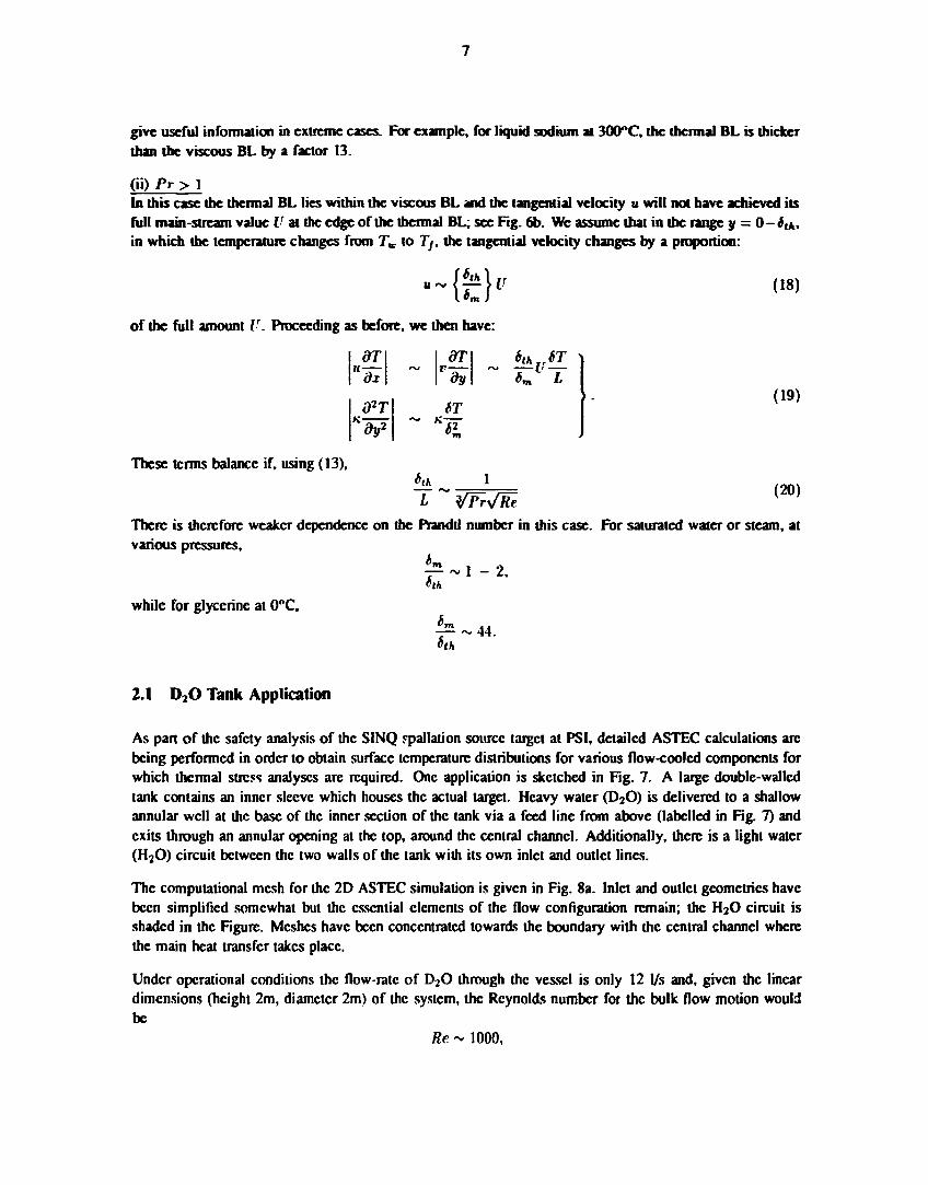
give useful information in extreme cases. For example, for liquid sodium at 300"C, the theimal BL is thicker than the viscous BL by a factor 13.

(ii) Pr > 1 In this case the thermal BL lies within the viscous BL and the tangential velocity u will not have achieved its full main-stream value U at the edge of the thermal BL; see Fig. 6b. Wc assume that in the range y = 0 - Stk, in which the temperature changes from Tw to Tj, the tangential velocity changes by a proportion:

l | rv m u (18)

of the full amount U. Proceeding as before, we then have:

dT

d2T

/Nrf dT

ST

*«A

*th *T )

4

1

(19)

These terms balance if. using (13),

T~VrWFe m

There is therefore weaker dependence on the Prandtl number in this case. For saturated water or steam, at various pressures,

6,k

while for glycerine at 0°C.

* M

1 - 2,

44.

2.1 D 2 0 Tank Application

As part of the safety analysis of the SINQ spallation source target at PSI, detailed ASTEC calculations are being performed in order to obtain surface temperature distributions for various flow-cooled components for which thermal stress analyses are required. One application is sketched in Fig. 7. A large double-walled tank contains an inner sleeve which houses the actual target. Heavy water (D20) is delivered to a shallow annular well at the base of the inner section of the tank via a feed line from above (labelled in Fig. 7) and exits through an annular opening at the top, around the central channel. Additionally, there is a light water (H20) circuit between the two walls of the tank with its own inlet and outlet lines.

The computational mesh for the 2D ASTEC simulation is given in Fig. 8a. Inlet and outlet geometries have been simplified somewhat but the essential elements of the flow configuration remain; the H 2 0 circuit is shaded in the Figure. Meshes have been concentrated towards the boundary with the central channel where the main heat transfer takes place.

Under operational conditions the flow-rate of D 2 0 through the vessel is only 12 1/s and, given the linear dimensions (height 2m, diameter 2m) of the system, the Reynolds number for the bulk flow motion would be

Re ~ 1000,

8

so that a laminar flow regime will prevail. Taking Pr ~ 5 for D 2 0 . the viscous and thermal BL thicknesses will be, respectively:

Sm ~ 3cm; S^ ~ 2cm.

The disposition of meshes along the inner tank wall and the inner sleeve are given in Figs. 8b, 8c, respectively. The wavy lines in the Figures signify the edges of the (conceptual) viscous and thermal BLs in the D 2 0 . The irregular mesh widths adjacent to the sleeve result from considerations of inlet and outlet details, not shown in the Figure.

The principal heat transfer surface is the inner sleeve; particularly at mid-height. Fig. 8b shows there are sufficient mesh points within the thermal BL to resolve the details of temperature profiles without recourse to the use of imposed heat transfer correlations. Steep thermal gradients arc not expected on the outer tank wall and the courser mesh seen in Fig. 8c is acceptable. Similar remarks apply to the expected velocity profiles within the viscous BLs, also marked in the Figures, and drag correlations arc not needed.

The remarks above refer to the bulk flow motion in the D 2 0 tank. Velocities at the inlet and outlet are higher and the respective Reynolds numbers based on appropriate hydraulic diameters are Rc(inlet) ~ 3500 and Re(ontlct) ~ 6300. Though mesh widths remain adequate for resolving laminar flow gradients, some mild turbulence may occur.

3 Turbulent Boundary Layers

3.1 Background

For high Reynolds number applications (Re Z 2000) turbulent motions can be expected. These can occur as a consequence of amplification of small pcrturbatioas in the bulk flow, or as a result of instabilities in shear and stratified layers. Turbulent motion is characterised by the presence of three-dimensional, irregular variations in the pressure, velocity and temperature fields. The paths of the fluid particles in turbulent motion are extremely complicated, resulting in extensive mixing of the fluid.

Turbulent motions take place at a multitude of scales ranging from the dimensions of the fluid enclosure L, down to the level at which molecular viscous action becomes important, /. It is shown below that

where Re is the bulk Reynolds number. As an example, for flow through a domestic cold water pipe. Re ~ 2 x 10s, and the length scales of interest will range from d, the diameter of the pipe, down to \0~4d. A direct 3D simulation of a section of pipe using the Navicr-Stokcs equations would therefore require of the order of If)12 mesh points to capture all the flow details. This is clearly impractical and alternative procedures must be employed.

The most common approach is to statistically timc-avcragc the conservation laws over time scales long compared to the turbulent fluctuations. This produces conservation-type equations for the mean variations. However, because the (molecular) conservation laws arc non-linear, the averaging process results in statistical correlations involving products of fluctuating quantities to appear in the mean flow equations. Such correla­tions cannot be determined directly from the solution of the averaged equations and further constitutive-type relations arc needed to close the system. Any particular model of turbulence supplies these missing relations.

9

Several approaches are possible (see Rodi [20] for a review), but we concentrate here on the (it - <) model as this is certainly the most popular, and the one which is implemented in the ASTEC code.5

In order to place the (it - 0 model in context, some discussion of earlier models is necessary. First ideas concerning turbulence modelling appear to date back to Boussincsq (1877) who suggested that the turbulent shear stresses in the averaged equations of motion, which arise from the cross-correlation of fluctuating velocities, be expressed in a similar form to the molecular «hear stresses in the Navier-Stokes equations [21 ]. For example, the shear stress r^, is expressed as

du Try = - P U V = // , — . (21)

in which fit is a new quantity termed the 'turbulent viscosity'. In this relation, u', v' refer to fluctuating velocity components in the i, y directions respectively, and ti is the mean x-component of velocity. Similar expressions pertain to the other stress components. Thus, if an expression for /i t can be obtained, (and. for heat transfer problems, an analogous expression for the turbulent heat flux) the system of equations is closed and the mean velocity (and temperature) fields may then be computed. Unlike fim, the molecular viscosity, / j , is not a fundamental physical property of the fluid, but will be largely determined by the state of the turbulence at, and probably upstream of, the locality.

Likewise, in the heat equation, a turbulent conductivity X, is introduced in order to relate the turbulent heat flux q" to the mean temperature gradient. Thus, for the ^-component:

dt tf = - r T ' = A , — , (22)

where V is the fluctuating temperature and f the mean value. A turbulent Prandtl number can also be defined:

crt = epp,/\t, (23)

and since the turbulent transport processes for vorticity and heat arc essentially the same, crt ~ I.

By analogy with the kinetic theory of gases. /i, is expressed in the following form:

/'« = r > ^ , . (2-1)

in which r,, (t arc characteristic velocity and length scales for the turbulence and c' is an empirical constant. The quantity (t is often termed the mixing length, and expression (24) the mixing-length hypothesis. Though dimcnsionally correct, it should be emphasised that there is really no physical justification for adopting the expansion (24) for the turbulent viscosity, nor indeed for expressing the turbulent stresses and heat fluxes in terms of mean velocity and temperature gradients, as is done in (21), (22). The derivation of the molecular equivalent of (24) in the kinetic theory of gases follows statistical arguments based on the existence of intermediate scales. That is, there exist length and time scales which arc small in comparison with variations in the mean quantities but arc large compared to the microscopic processes which determine the momentum and heat transport — the continuum hypothesis. The existence of intermediate scales is central to the statistical averaging procedure in ensuring that the derived properties arc local, and independent of the mean-flow characteristics. Isotropy at the local level follows from the random nature of the molecular interactions.

Turbulent motions, even fully-developed ones, possess none of these characteristics. As already remarked, fluctuating turbulent motions exist at many scales, up to that of the fluid enclosure. There arc no clearly-defined intermediate scales separating the mean and fluctuating variations. Consequently, the averaging

sAn algebraic stress model for ASTEC is currently in development.

10

process applied to turbulent flow is not well-founded, large-scale information is lost, there Is no guarantee that local effccLs depend only on local properties, and isotropy cannot a priori he assumed. However, all these considerations arc ignored in the mixing-length hypothesis in the expectation that the resulting model will at least give a usable approximation to the actual mean-flow behaviour in lieu of actually solving the full, non-avcragcd equation set.

The turbulent viscosity [tt is taken as constant, for simplicity, in the original mixing-length model, but later Prandtl (22] suggested relating the turbulent velocity. vt in (24), to the mean flow gradient via the relation

. I«">« l r. = f,|— . (23)

and correlating the remaining parameter ft from the flow geometry. Later still, von Karmin [231 proposed

' / = ihj i)y2 (26)

which alleviated the problem of prescribing (t for each situation, but results were not in accord with experi­ment, except for flow near walls. Further, for turbulent jets and mixing layers.

i)2u

0y2 = 0

at approximately the position of maximum shear stress. This point represents a singularity in die von Kärmän model and the maximum value cannot be calculated.

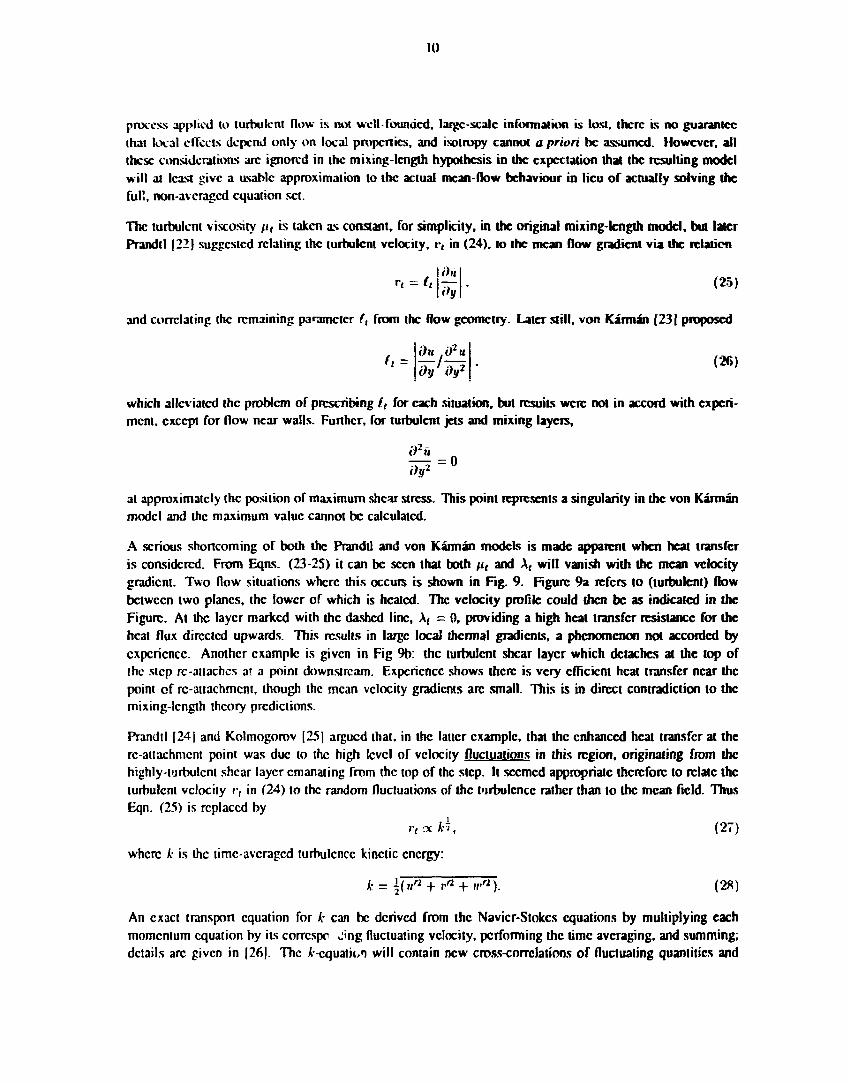
A serious shortcoming of both the Prandtl and von Kärmän models is made apparent when heat transfer is coasidcrcd. From Eqns. (23-2S) it can be seen that both fit and A, will vanish with the mean velocity gradient. Two flow situations where this occurs is shown in Fig. 9. Figure 9a refers to (turbulent) flow between two planes, the lower of which is heated. The velocity profile could then be as indicated in the Figure. At the layer marked with the dashed line. A, = 0, providing a high heat transfer resistance for the heat flux directed upwards. This results in large local thermal gradients, a phenomenon not accorded by experience. Another example is given in Fig 9b: the turbulent shear layer which detaches at the top of the step re-attaches a? a point downstream. Experience shows there is vciy efficient heat transfer near the point of rc-aitachmcnt, though the mean velocity gradients arc small. This is in direct contradiction to the mixing-length theory predictions.

Prandtl [24] and Kolmogorov [25] argued that, in the latter example, that the enhanced heat transfer at the re-attachment point was due to the high level of velocity fluctuations in this region, originating from the highly-turbulent shear layer emanating from the top of the step. It seemed appropriate therefore to relate the turbulent velocity r, in (24) to the random fluctuations of the turbulence rather than to the mean field. Thus Eqn. (25) is replaced by

» ' , «** , (27)

where k is the timc-avcraged turbulence kinetic energy:

k = \(n" + t* + w"). (28)

An exact transport equation for k can he derived from the Navicr-Stokcs equations by multiplying each momentum equation by its corrcspo Jng fluctuating velocity, performing the time averaging, and summing; details arc given in [26]. The A-cquati»,n will contain new cross-correlations of fluctuating quantities and

11

these must be related back to the mean-flow variables in order to close the equation set. We write here the it-equation (in symbolic form only) as:

^ = D + P + G-(, (29) at

in which the lhs represents the derivative following the motion. Thus, the rate of change of k along a streamline is determined by:

(1) the diffusive transport as a consequence of velocity and pressure fluctuations, D;

(2) the production of k due to the work done by the Reynolds stresses, P;

(3) the work done by the buoyancy force, G;

(4) the dissipation of k into heat by viscous action, e.

Such models go under the collective name of one-equation turbulence models and give improved predictions for flow and heat transfer in ducts and for separated flow. However, there remains the problem of specifying the mixing-length tt in (24).

A further development is to derive lt itself, or an equivalent turbulent propety, via a second transport equation. The (k - t) model is one such two-equation turbulence model in which the second variable is chosen to be t, the turbulence energy dissipation rate. The choice lies partly in the ease with which a transport equation for e can be derived from the exact equations, and partly in the fact that e already appears directly in the transport equation (29) for k. Further discussion of the particular benefits of the (k - e) choice is given by Launder and Spalding [11]. An exact transport equation for e may be derived from the Navier-Stokes equation for the fluctuating vorticity. Again, several additional closure assumptions are necessary before the equation is tractable; see [27] for details of the derivation.

With k, i determined via their respective transport equations, the mixing-length tt needed in Eqn. (24) follows immediately from the Kolmogorov relation:

tt = cDk2/e, (30)

with cD a universal constant. This relation too is based on simple, dimensional arguments. As already stated, the mean dissipation of turbulent energy, e, takes place at the smallest scales due to the direct action of the molecular viscosity fim. However, the energy itself is derived from the largest eddies. Hence, /zm

will define Üu ultimate scale at which the dissipation takes place, npi the degree of dissipation. It follows that the magnitude of e is determined by those quantities which characterise the largest eddies. These are the mixing-length £,, and the turbulent velocity, ki in the present model. The expression (30) is the only combination of these quantities giving the correct dimensions.

An estimate of the scale I at which 'he turbulent dissipation c takes place as a result of molecular viscous action also follows from similar dimensional arguments. The only quantities which can determine the scale I are the fluid density p, the mean dissipation rate itself e, and the molecular kinematic viscosity v. The only combination of these quantities giving the correct dimensions is

l~V-T- (31)

12

The mixing-length lt in (30) is associated with the largest turbulence scales, and these we have seen are characteristic of the length-scale L of the mean motion. Hence, we can re-cast (31) in the form:

(JJ * * ry ( 3 2 )

Since the mean turbulent kinetic energy k is determined primarily by the motions at the largest eddy scales, the fluctuating velocities are of the same order as the changes in the mean flow field occurring over the distance L. It follows that the inverse of the expression in brackets in (32) would be a good definition of the bulk Reynolds number Re. Hence, we have

l~LjRe$, (33)

the estimate for the smallest eddy scales quoted at the start of the section.

The high Reynolds number Kk - c) turbulence model (with buoyancy) is programmed into the ASTEC code. Thus, in addition to the usual conservation equations for mass, momentum and energy, the transport equations for k, ( must be solved simultaneously. The procedures are described in [29]. Modifications to the model are required close to solid (no-slip) boundaries where local Reynolds numbers become small. Though low Reynolds number (k — c) models have been proposed [10,11], a popular alternative is to use universal wall functions [12], to which the solution in the far-field is matched. This is the procedure adopted for ASTEC.

3.2 The Wall Function for Turbulent Shear

The Law of the Wall was originally derived on dimensional grounds by Prandtl [30], and von Kärmän [23]. The main arguments arc sketched out here for the sake of completeness. Consider turbulent flow over a heated, stationary plate, as depicted in Fig. 10. The frictional force/unit area due to turbulence, r, is just the tangential component of momentum transmitted towards the surface per unit time. For the flow direction defined in Fig. 10, the force is clearly in the negative x-direction and arises as a consequence of the mean tangential velocity gradient (dü/dy) in the layers next to the wall, though outside the laminar sub-region along the wall where the molecular viscous forces dominate. If there were no gradient with respect to y, the co-ordinate perpendicular to the surface, there would be no net momentum flux and no drag due to turbulence. Outside the viscous sub-layer molecular viscous forces may be ignored so that the factors determining the magnitude of r are the velocity gradient (dü/dy), the density p and the distance from the wall y. The only combination of these variables giving the correct dimensions is:

K"W"*i- (34)

where the proportionality factor \ (=0.42) is called von Kärmän 's constant and is estimated based on velocity gradient measurements for turbulent pipe flow.

Near the wall, but still outside the viscous sub-layer region, the turbulent momentum flux — like the heat flux — can be treatul as a constant TW, the frictional force per unit area on the plate surface due to turbulence, and (34) then integrates giving:

u* u = — (In y + c) (35)

in which

«* = (rjptf (36)

13

is an effective turbulent shear velocity and c is a constant of integration to be determined by application of a suitable boundary condition. This cannot be applied at the wall itself (y = 0) since (35) has a singularity there, reflecting the neglect of molecular viscosity during the derivation. Likewise, there is no sensible condition at infinity, where the formula is again singular. Instead, a suitable point is chosen near, but not at, the wall.

An important consequence of the above dimensional arguments is that the velocity u* must characterise the scale of the fluctuating velocity of the turbulence independently (to leading order) of the distance y from the wall, since it is not possible to derive any other quantity having the dimensions of velocity from the three variables TW, p, y . Hence, at a distance ya from the wall, the local Reynolds number must be of the form:

Re' = u'yjv (37)

where v is the molecular kinematic viscosity. Viscous effects become important for Re ~ 1, and this will occur at the distance

Vo ~ v/u* (38)

from the wall, which becomes a measure of the extent of the viscous sub-layer for the wall model. Formally setting u - u" for y = y0 in (35) determines the constant of integration c, so that finally:

u = — ln{Eu'y/v) (39) A

in which the proportionality constant in (38) has been absorbed into the parameter E. This is usually termed the Roughness Parameter and the value E = 9.0 is generally adopted for a hydraulically smooth surface [31,32].

The relation (39) is conveniently written in dimensionless form as:

u+ = -\n(Ey+), (40)

in which u+ = u/u*; y+ = u'yfv. (41)

The logarithmic velocity profile is well confirmed by experiment for the range:

30 < y + < 100, (42)

which is well outside the viscous sub-layer (y+ ~ 1) but not so far that the mean velocity becomes significant compared to u*.

In fact, for non-separated flow, the Reynolds stresses remain approximately constant over this range and it is easy to show that this condition is equivalent to fc=const. by the following i .guments: For k constant it follows from the transport equation (29) that, neglecting buoyancy forces, there is a balance between the production term P and the dissipation term e. That is, using (30),

_ du ki P = TW— = cDp— = e.

dy It

Multiplying both sides of this equation by the turbulent viscosity fit = c'ßpk*tt, end remembering that

rw = ptfy, (43)

14

it follows that: {TW/P)2 = c^k? - const. (44)

where cM = c'ßcD (=0.09) is an empirical constant estimated from experiments [28]. Some practitioners

use the above equality to replace the shear velocity u* = ( W P ) 2 in the wall Equation (39) by one of the following:

7i* = c^fc2, or u* = (Tw/p)/c£k2, (45)

or a combination of both. The first definition is claimed to give more plausible predictions in non-equilibrium (P ^ f) situations. In particular, at points of flow separation and re-attachment, r,„ — 0 whereas k remains finite. A combination of the two alternatives in (45) has been adopted in ASTEC. More of this later.

3.3 The Wall Function for Turbulent Heat Flux

Analogous arguments to those presented in the last Section, which led to the law of the wall (40) for the near-wall velocity, can also be used to derive a law of the wall for the mean temperature profile in turbulent heat transfer. In dimensionless form, this is

T+ = ^ln(Ey% (46) A

in which the temperature scaling is given in terms of the wall superheat according to

T+=pcp(Tw-T)u'/ql (47)

with cp the specific heat and <?" the wall heat flux in the normal direction. Lateral heat exchange is assumed negligible through the near-wall layers giving, at a general point, q"{y) = q'w = const. The parameters \, E appearing in (46) are the thermal equivalents of the von Kärmän and roughness constants x» E. The logarithmic temperature profile is well confined by experiments.

As an alternative to separately determining the new parameters \, E, it is often convenient to combine the velocity and temperature wall expressions (40), (46) giving

T+ = 4 (U+ + V) (48)

in which the pee function,

V = -\n(E/E), (49) A

has been correlated from p'oe-flow data by Jayatilleke [33], as

V = 9.24 (<j< - l) (1 + 0.28exp [-0.007a]), (50)

with Ö = -CT, (51)

A

and a - wcp/A, the molecular Prandtl number.

15

3.4 Use of Wall Function Treatment in ASTEC

The laws of the wall for the velocity and temperature fields arc applicable only to the near-wall layers, but lying outside the viscous svtb-lnycr immediately adjacent to the wall. The implementation of the wall treatment in the ASTEC code is described elsewhere (13,29), and it remains here only to comment on the placement of the mesh in the wall vicinity to ensure consistent use of the model.

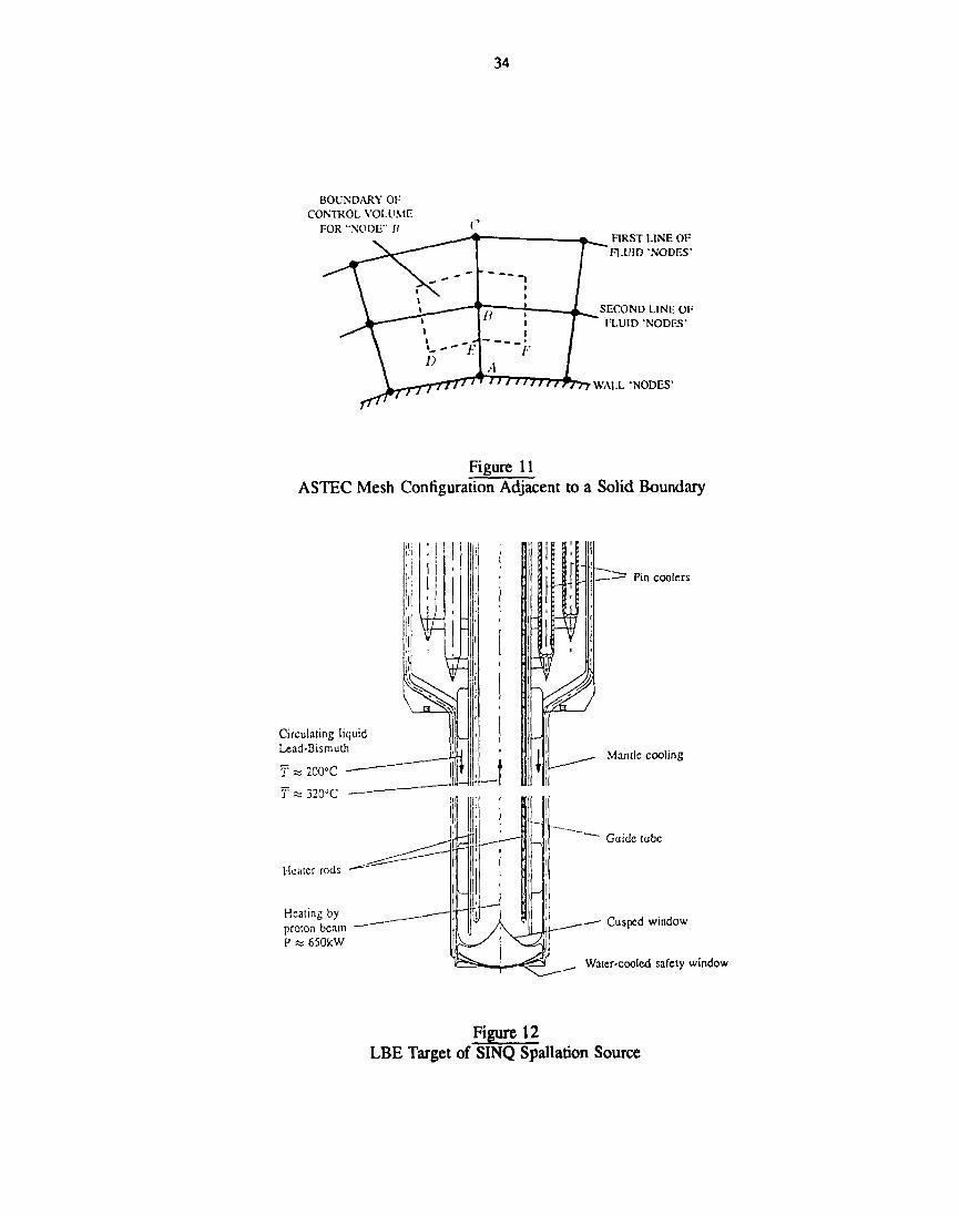
Figure 11 shows, in 2D, a typical mesh configuration in the proximity of a solid boundary. It is always possible, and advisable, with ASTEC to orientate the mesh in approximately rectilinear form in the fluid layers next to the wall surface. The governing equations of motion, including the transport equations for the turbulence quantities k,« arc integrated over control volumes surrounding the nodal points:- a typical control volume is indicated in the Figure.

Rates of change of mass, momentum, energy, k and t within each control volume arc determined by changes due to volumetric sources within the volume, together with the fluxes (convcctivc and diffusive) of respective quantities across the control volume boundaries. For internal fluid nodes, such as node C in Fig. 11, the fluxes across the control surfaces arc estimated using interpolation from nearby nodal values. This is adequate provided the flux quantities vary smoothly through the mesh. However, in the near-wall region, where large velocity and temperature gradients occur, this approach has to be abandoned. Thus for node B, next to the wall, the flux terms over the surface DEF are estimated using the wall function model. Strictly, this means that at the point E the normal momentum flux r£ should be determined directly from the law of the wall (39). ASTEC appears to adopt the first scaling factor for «• in (45) inside the logarithm, and the second factor outside. This would give:

In \EyEclkllv\

where ijK is the distance of the control surface from the wall and kE is the turbulent kinetic energy at E. In fact, a s'ightly modified treatment is coded since the velocity uE is not directly available — the velocities arc known only at the nodal points — and no interpolations can be used due to the large gradients. Instead, the momentum flux is evaluated at the node B according to

l l

r pkBuBXcl TE ~ —7 T1—7' W2)

Ir In \FAjBclkljv\

but then applied to the control surface DEF. This is reasonable provided that B itself lies within the range of validity of the wall function treatment, Eqn. (42). Thus, to ensure that the near-wall treatment in ASTEC is legitimately applied it is necessary to place the first line of fluid nodes at a distance yB from the solid surface, where

30 < c$kiyB/v < 100. (53)

The user is responsible for ensuring that the condition is satisfied: there arc no internal checks within the code.

Similar arguments to those presented apply also to the specification of the heat flux q'E at the control surface DEF. As before, this is evaluated at the node B, where the temperatures arc known, rather tha.. at E itself, on the assumption that q'E is constant in the near-wall layers. In this case, the first scaling factor in (45) is

16

used which gives, in dimensional form:

i i „ pcPxclkl{TA-TB) ....

ie = j—7 r r ^ \ T' (54)

in which 7^, 7 B are the nodal temperatures at A, B. The same condition (53) applies for the heat flux determination.

In order to provide a practical way of determining where to place the ASTEC mesh in the (turbulent) fluid layers next to a solid boundary, we re-cast some of the formulae derived so far in more useful forms. If the first line of fluid nodes is placed a distance yj from the (heated) wall, and L, U are typical length and velocity scales tangential to the wall, then after some manipulation of Eqns. (40), (41) it can be shown that the boundary layer co-ordinate y+ satisfies

y \n(Ey+) = XReyj/L, (55)

where Re = UL/u is the Reynolds number for the main-stream tangential flow. Solving this equation for j / + one can then check whether

30 < y+ < 100,

as required by the wall function treatment. An example follows.

3.5 Application

The SINQ spallation source is designed for continuous thermal neutron production by the bombardment of a target by a 570Mev proton beam. Accompanying the spallation reactions, large amounts of heat arc produced (~640 kW) and an attractive design option is to use a long column of heavy liquid metal (e.g. lead or lead cutectic) as the target and rely on natural circulation currents within the liquid to transport the heat generated in the spallation region upwards to secondary coolers, Fig 12. The feasibility of the cooling arrangement' •; being examined using the ASTEC code and, to complement these studies, validation tests have been devised using liquid sodium as simulant coolant.

The first of the Target Cooling Simulation, or TACOS, tests aims to verify ASTEC code predictions of the temperature distributions over the window, the profiled, steel plate at the base of the liquid metal column, through which the proton beam passes. Figure 13 shows a schematic of the TACOS test configuration. Sodium enters the test section via inlet chambers at the top and, after passing through a flow resistance, descends in the outer annular region to a cusp-shaped, heated plate at the base of the vessel and then up the central channel to the outlet.

Pre-test ASTEC calculations have been performed as part of a basic scoping study and to give guidance on the positioning of instrumentation in the experiment. The ASTEC mesh, given in Fig. 14a, is moulded to the test geometry and aims to capture details of the developing turbulent flow over the heated surface of the window. Under conditions of maximum inlet flow (10kg/s) and maximum heating (10kW) the bulk flow Reynolds number is estimated as

Re ~ 4 x 105.

The viscous sub-layer next to the window surface is estimated from experiments [2f] io extend from y+ = 0 to y+ ~ 5. Using (55), the viscous sub-layer thickness would rx

f>SL ~ 0.02mm.

17

The thermal sub-layer thickness is usually assumed to be of similar magnitude, since the turbulent Prandtl number at ~ 1, though could be slightly narrower for liquid metals.

For comparison purposes, if the buik flow were laminar at this value of Re, the viscous and thermal BL thicknesses would be, according to (13): (17):

6m ~ 0.12mm; 6th ~ 1.5mm.

The disposition of the mesh in the proximity of the window surface is given in Fig. 14b. The first line of fluid nodes, which is at a distance yj = 0.17mm from the wall, corresponds to y + ~ 52, according to (55), and hence satisfies the criterion (42). The second line of nodes corresponds to y + ~ 134 and this lies outside the turbulent boundary layer. It follows that the standard, large Reynolds number (k - e) model can be used legitimately with this mesh placement.

4 Use of Heat Transfer Coefficients in ASTEC

Options exist for user-defined drag and heat transfer correlations to be introduced into the discretised transport equations solved by ASTEC. This is particularly useful for flow through porous media where standard correlations are available, e.g. [34,35], for a variety of fine-scale geometries. The option is also useful however, for open flow (Porosity = 1 ) conditions near boundaries where the computational mesh is too coarse either for the details of the laminar BL profiles to be discerned, or for the wall function turbulence model to apply. In these circumstances, it is necessary to supply external drag and heat transfer data to correlate the bulk flow velocities and temperatures with the wall values.

Adequate instructions are given in the ASTEC input manual [13] for introducing drag correlations, for all internal and external fluid/solid boundaries, and need not be repeated here. It is also straightforward to introduce a heat transfer correlation between a solid surface at a known temperature and the adjacent fluid; details again in [13]. By a slight extension, a constant heat flux boundary condition is also easily handled. However, ASTEC is able to calculate heat transfer by conduction through solid regions and, if this option is invoked, care is needed in the implementation of solid-to-fluid heat transfer correlations.

The problem can be explained in a simplified, two-dimensional context with reference to Fig. 15a, which shows a coarse mesh configuration near the boundary between a hot solid and adjacent moving liquid. The temperature profile along the line of nodes CAB might resemble that given in Fig. 15b, for example. Heat transfer within the solid region is by conduction alone, while in the fluid region (laminar and/or turbulent) convective heat transfer also takes place. As Fig. 15b indicates, the mesh is here too coarse to resolve explicitly the temperature profile in the liquid layers adjacent to the boundary and it will be necessary to input an external heat transfer relation to correlate the normal heat flux at the wall q"A to the temperature drop (TA - TB). This is usually done in terms of a heat transfer coefficient h according to:'

qA = h(TA-TB), (56)

where, for the standard definition of heat transfer coefficient, TA would be the wall temperature and 7g the bulk fluid temperature. If turbulent flow conditions prevail in the far field, it will be necessary to by-pass the wall function treatment in the code by modification of the wall function routine (WALFNT for ASTEC

'Note that h used in this expression is the usual heat transfer coefficient with units W/M2K. The quantity h which appears in the ASTEC input manual [13] in this context relates to a volumetric source and has units W/M3K.

18

version 1.4B). If the bulk flow is laminar, wc will assume that the heat flux arising from molecular diffusion from the wall is negligible compared to the q"A in (56), otherwise steps will have to be taken to remove it.

In order to solve the discrete equations resulting from integrating the transport equations for mass, momentum, energy (and additionally for k, ( if the turbulence irodcl is tcing used) over the nodal control volumes (two such volumes arc shown in Fig. 15a), ASTEC invokes an iterative solution procedure based on the SIMPLE [5] algorithm. The algorithm converges only if the solution matrices arc diagonally-dominant. Relaxation factors, minimum values of which arc user-controlled, are introduced to ensure such dominance exists. The method normally works well but convergence is slow for stiff systems which result if one of the off-diagonal terms is of comparable size to the diagonal term, and is not easily improved by redefining relaxation factors. This situation can arise as a consequence of user-input heat transfer correlations. This point is taken up later.

Details of the iterative procedures in ASTEC arc adequately described in the code documentation [13], but the basic principles will be sketched here for the sake of continuity. Each iterative step J begins with a guess at the pressure field p'J* throughout the fluid domain. Usually, the pressure at the previous iteration (with optional undcr-rclaxation) is used. The linearised momentum equations arc then solved by multiple sweeps using pointwise, successive-ovcr-rclaxation (SOR), with a Jacobi iteration for the first sweep. This scheme reduces to standard Gauss-Seidcl if the relaxation factor is unity. Having computed, for the given pressure distribution p^J\ the 3-D velocity field {u^J\v^J\w^), within a specified tolerance, the next step is to check whether mass continuity is satisfied, again to within a specified tolerance. In general, the computed velocity field will violate the mass conservation condition and spurious mass sources (or sinks) would need to be introduced to maintain mass balance. The second step of the solution procedure is to introduce changes to the velocity field (Su^KSv^^Sw^), sufficient to eliminate the spurious mass sources. Writing the velocity changes in terms of pressure changes 6p^JK using the incremental form of the momentum equations, enables a Poisson-type equation for the ip^ to be formulated. This is solved iterativcly to within a given tolerance using a pre-conditioned (the Poisson matrix is non-symmetric), conjugate gradient method.

Next, the transport equations for energy, the turbulent quantities k, e, and any other scalar function (e.g. concentration) arc solved in a similar way to the momentum equations, each with their own relaxation parameters and convergence criteria. The entire process is repeated until all the convergence criteria are satisfied simultaneously.

Restricting attention to the computation of the temperature field within the iteration scheme, the discrctised energy conservation equation may be written in the general form for the ith node:

«» i>i

in which T, is the temperature (for the given iteration) at node i, and the summations are taken over all nodes which share an element with the node i. In the framework of the SOR scheme, all temperatures on the rhs of (57) arc latest values. The first summation, for / < i, is over those nodes which precede i in the SOR sweep. The superscript (./) signifies that for such nodes the temperature has already been updated within the current iteration. The second summation, for I > i, is over those nodes which follow i in the SOR sweep. The temperatures at such nodes have yet to be updated within the current iteration; hence the superscript (./ - 1). The dimcnsionlcss coefficients a„ bu, arc calculated according to the contributions arising from the advective and diffusive heat fluxes, while c,i, which has the dimensions of temperature, is made up from heat source terms and previous cycle quantities.

In order for successive sweeps of his equation to lead to a convergent solution for the Tj, it is necessary

19

that

kl > £ IM for **'nodes '• (58) Vi

In other words, the diagonal entry must be at least as large as the sum of the off-diagonal terms, and there must be strict inequality for at least one rode. If these conditions are satisf cd the SOR scheme will converge. However, the rate of convergence depends on the distribution .f the 6,;'s: if one entry in the matrix row becomes comparable in size to a„ convergence is seriously impaired.

There are three options for implementing heat transfer correlations in the ASTEC code. These we refer to as

(i) Explicit: previous cycle temperatures used in (56);

(ii) Jacobian: previous iteration temperatures used in (56);

(iii) Implicit: current cycle temperatures used in (56).

Each case above will be examined with reference to Fig. 15a. Using (57), the discretised energy equations for the wall node A (node number = i) and the fluid node B (node number = j) at the Jth itcratior may be written as follows:

a,TJJ) =-6, JT J ' 7 - 1 ) - E i < > T / - ' ) -D> , f c /T / J - 1 ) +c, Wall Node A

a3TJJ) = -b]%T\J) - £ ( < J 6 j ,r/J ) - D > , b}lT\J-x) +Cj Fluid Node B (59)

in which the particular interaction between the two nodes i, j has been emphasised by extracting the ap­propriate factor from the general summation terms. Without loss of generality, it has been assumed that : < j .

During the time step St an amount of heat SQ is transferred from the wall node A to the fluid node B, where

6Q = Aq"fil = Ahbt{Tt - Tj), (60)

and A is the area of the control surface FGH in Fig. 15a. The three implementation schemes itemised above stem from the different assumptions made for the temperatures in the expression (60).

4.1 Explicit Scheme

This is conceptually the simplest approach, in which the nodal temperatures TJ \ 7'- ' at the previous cycle arc used in (60). The heat exchange between A, B then remains constant during the inner iteration sweeps within the cycle and can be included in the source terms in (59) as follows:

< = a - Ah6t.(Tl0) - TJ0))/pcp

d3 =cJ+Ah6t(Tl0)-TJ0))/pcp

(61)

in which p, cp arc the density and specific heat capacity of the fluid, and p, cp those of the wall material. The SOR iteration sweeps then proceed as normal.

20

Though the explicit approach has the benefit of simplicity, the main disadvantage is that there will be a stability limit for the time step St. A simplified stability analysis is given in Appendix 1 and yields the following criteria. For the wall node A, if

h < ^r, (62)

the scheme is stable. Here, A is the thermal conductivity of the wall material and 6y is the mesh width in the wall perpendicular to the heat transfer surface. The criterion, which is independent of time step, states simply that the heat exchange via the heat transfer correlation must be smaller than that due to conduction, there being no convection effects. In other words, the implicit part of the calculation (conduction) must dominate over the explicit component (heat transfer correlation) to preserve stability.

However, if h represents the dominant heat transfer process, and the condition (62) is violated, the heat exchange between the wall and fluid nodes A, B must not take place on a shorter time scale than that determined by the physical process of conduction. Hence we can anticipate a time step restriction on the imposed heat transfer process. The analysis in Appendix 1 shows this to be:

6t<-~ 2 h - X/Sy

(63)

in which 6y is the mesh width on the fluid side of the heat transfer surface, other symbols have the usual meanings, and the tilde signifies that the physical property pertains to the wall material.

Examining now the stability of the solution process for the control volume centred around the fluid node B, if the following condition is satisfied:

h < — - pcpVj , (64)

in which Vj is the velocity perpendicular to the wall at the point J in Fig. 15a, the scheme is stable for all values of the time step. This expression is the analogue of (62) for the fluid: the factors X/6y and pcpVj represent heat transfer effects by conduction and (vertical) convection respectively, both of which are handled implicitly by ASTEC. These effects can maintain numerical stability provided the heat transfer via the correlation h is not too large.

However, if condition (64) is violated, there is a time-step restriction given by:

6t < pcp6y(h + pcpVj + X/Sy)

hi _ {X6y - pcpVjf (65)

Since the explicit method only results in changes being made to die source terms in the equation &ct (59), the rate of convergence of the iteration sweeps within a cycle is unaffected. Provided the criteria (62)-(65) do not result in prohibitive restrictions, particularly with regard to the time step, the scheme is workable in ASTEC and requires no changes to the code.

4.2 Jacobian Scheme

In this method the nodal temperatures TJ ~ , TJ _ 1 ' at the previous iteration are used in the imposed heat transfer expression (60) and are only updated at the end of the current iteration sweep. This means that the factor -b3iT\J) in the second of the equations in (59) is replaced by -bjiTJJ~^ degrading the SOR iterations to Jacobian for the fluid nodes next to the heated wall. The stability of the iteration scheme within a cycle

21

may be examined using a similar analysis to that given in Appendix 1 but with the cycle number n replaced by the iteration number J. This will lead, for the special case in which the relaxation parameter ui - 1 (no relaxation), to the same stability criteria (62)-(65) derived for the explicit case. However, if over-relaxation (UJ > 1) is used it has been shown (in an analysis not included here) that the stability criteria arc much stricter than for the u; = 1 case, and can lead to unconditional instability if the heat transfer coefficient h is large. Consequently, this scheme is not recommended.

4 J Implicit Scheme

If current cycle temperatures Tt , T arc used in (60) the scheme is fully implicit and there will be no restriction on time step size, at least from the standpoint of numerical stability. The heat exchange between nodes A , Ii is directly incorporated into the overall iteration scheme (59) by appropriately modifying the coefficients of 7 ' / ' ' , T- according to the following prescription:

n- = a, + Ahf>t/pcp

b'l} = btJ - Ahdt/pcp

a'j = dj + Ahttfpcp

b'}, =bji-Ah6t/pcp

} • (66)

Note that for each equation in (59) the same term is added to both sides of the equation. Hence, the inequality (58) remains valid and the SOR iteration scheme will still converge. However, if the heat exchange represented by the heat transfer coefficient h is the dominant heat transfer process, the additional terms in (66) will be larger in absolute amount than the original coefficients, and

\<\ ~ 1^1 ~ \Ah6t/pcp\ ) (67)

l«SI ~ K.I ~ \^6t/pcp\ J In other words, for those rows of the solution matrix representing wall and fluid nodes of the type A, B in Fig. 15a, one off-diagonal entry will be of similar magnitude to the diagonal term. The matrix system would then be stiff and we would anticipate accompanying deterioration in the rate of convergence of the SOR scheme. The principle is best illustrated by means of a specific example.

Consider the case of pure heat conduction in 2-D on a square lattice, as shown in Fig 16a. The governing equation which, under steady-state conditions, reduces to

0 = M ^ + ^ i W ' , (68)

with q'" the volumetric power density, is integrated over each nodal control volume to give the discrctiscd energy equations for the system. For the two nodes A(i,j) and 7?(J, j + 1) in Fig. 16a, these would be:

, ( 6 9 )

where the temperature has been scaled in order to make the source term unity. For the matrix system derived from (69), each diagonal entry {4} would equal the sum of the off-diagonal terms {1 + 1 + 1 + 1}.

22

If we now impose an additional heat transfer from node (t, j ) to node (i,j + 1) of, in scaled quantities,

i f ^ - T . j + j ) , (70)

in which the factor H is the scaled equivalent of the heat transfer coefficient h, the Eqns. (69) are modified to:

(4 + / o r , , , = Tt.hj +i;-J-_, + r l + 1 J +(i + H)Tid+1 +1 ) \ (71)

The overall balance of the diagonal to the sum of the off-diag jnal terms is not disturbed by this addition, but one of the off-diagonal terms now dominates the others and, if H > 1, becomes comparable to the diagonal te;m on the lhs. In order to see the effect of this on the convergence rate of the SOR iteration scheme, a small interactive computer program has been written based on the equation set (71). A listing of the program is given in Appendix 2 and sample results are displayed in Table 1. The Table shows clearly (in the third column) the lack of convergence for increasing values of H. It is also evident that there is only limited improvement with adjustment of the relaxation parameter, and the optimum relaxation is also H dependent.

Heat Transfer Parameter

H =0.0

// = 10.0

H = 100.0

H = 500.0

Relaxation Parameter

w= 1.00

w = 1.75 (optimum)

w= 1.85

w= 1.93

u= 1.97

w= 1.00

u/= 1.75

a/= 1.85 (optimum)

w = 1.93

u= 1.97

u>= 1.00

w= 1.75

u= 1.85

u = 1.93 (optimum)

w= 1.97

u>= 1.00

w= 1.75

u= 1.85

u>= 1.93

u = 1.97 (optimum)

Number of Iterations (Standard Case)

tf=205

JV = 26

iV=45

iV = 94

iV = 229

# = 4 1 5

N = 7S

N = 46

JV=93

JV = 209

N = 1555

iV = 386

iV=240

jV = 82

iV = 200

N = 2919

JV = 1214

JV = 817

# = 435

JV = 209

Number of Iterations (Augmented Case)

N= 178

JV = 29 (optimum)

iV = 48

N= 100

# = 236

N= 167

N = 28 (optimum)

JV = 46

JV = 98

# = 226

N= 165

N = 27 (optimum)

# = 45

# = 97

# = 228

# = 165

# = 27 (optimum)

# = 45

# = 97

# = 229

Number of equations = 25, tolerance for convergence = 0.01

Tabic 1: Rates of Convergence for Sample Problem

23

(72)

In order to improve convergence for large H it proves useful to augment tiic standard SOR iteration sweep with a local simultaneous solution procedure between the two dominant terms in (71): that is. for the terms representing the two nodes A, 11 between which the main heat exchange takes place. A similar procedure has been used successfully by the author in the past [361. and also appears in the two-phase versions of PH0EN1CS [371 and FL0W3D [381 under the acronym PEA (Partial Elimination Method) to alleviate slow convergence problems associated with tight coupling between the phases. The basic idea is to locally solve the equation set (71) as a 2 x 2 linear algebraic system with unknowns T,,r 7*;J+1. Thus, wc eliminate the 7"ij41 term from the first of the equations, using the second, and the TU] term from the second, using the first. This gives:

3(5 + 2H )7/t j = (4 + 11) [(Tt.Uj + 7,.,.., + 7,+ I J

+ (1 + l / ) [r ,_ U l _ , + ri+Uj+t 4- T,.,+2] +(5 4 21/)

3(5 + 2 / / ) / , . , + 1 = (1 + H)[(rt_Uj + / , , _ , + 7-,+Ij]

+ ( i + / / ) [ 7 , - , . ^ , + / ;+, . J + ! f 7 ; . ; + 2 j +(o + 2W)

The diagonal entry in the matrix system derived from (72) is again equal to the sum of the off-diagonal terms, but these arc now more evenly distributed, for all values of // . This augmented scheme is included in the demonstration program given in Appendix 2. and Ihc improvement it brings to the convergence rate of the SOR procedure is shown in the last column of Table 1. As the Table shows, there is now no penalty on convergence for increasing values of //. Indeed, the optimum relaxation parameter for maximum convergence efficiency remains unchanged. This represents a significant improvement over the standard scheme.

The implicit formulation therefore, coupled with the augmented SOR iteration method, looks the most attractive of the three schemes considered, but necessitates some minimal code modifications to accommodate the additional entries in the solution matrix required by (72). It should be noted however, that the analysis carried out here is for smooth surfaces in which it is always possible to ascribe a unique fluid node, B, to every wall node. A, where the imposed heat transfer is to take place. At angles and corners, see Fig. 16b. more nodes arc involved and some further code logic will be needed to select the dominant coefficients in the solution matrix for the local 2 x 2 simultaneous solution. Heat transfer correlations would, in any case, be untrustworthy for such configurations and it is questionable whether the extra programming effort is worthwhile.

5 Final Summary

The ASTEC code utilises a discrete, finite volume algorithm to solve the equations of fluid dynamics and heat transfer on an unstructured mesh. The placement of the mesh in the vicinity of no-slip boundaries to derive maximum information with regard (o prevailing velocity and temperature profiles is described in the text. Derived criteria, based on a dimensional analysis of boundary layer behaviour, translate into practical hints for ASTEC users and arc summarised as follows:

• For laminar flow conditions, Reynolds number fir < 2000, respective thicknesses fim, filfl of the viscous and thermal boundary layers may be estimated in terms of the tangential length scale /, according to:

b» _J_

24

and ttk 1

Stk 1

for Pr< 1;

iorPr> 1.

where Pr is the molecular Prandtl number. It is recommended that at least three mesh points be placed within the layers to resolve the velocity and temperature gradients reliably.

• Under turbulent flow conditions. Re ^ 2000, the distance yj between the boundary and the first line of fluid nodes should be chosen in order that the solution y+ of the following transcendental equation:

y+ln(Ey+) = XReyj/L,

in which E (= 9.0), \ (= 0.42) are the roughness and von Karmin constants respectively, satisfies the criterion:

30 < y+ < 100.

If the line of fluid nodes is placed outside the laminar and/or turbulent boundary layers, according to the above cnteria, it will be necessary to impose external drag and/or heat transfer correlations to supply the missing boundary layer information. ASTEC does not calculate the motion of solid structures and the introduction of drag coefficients does not result in strong coupling between the fluid and structural nodes. Likewise, imposed heat transfer from a solid surface at a given temperature presents no problem. Details for these ca^cs are described in the ASTEC User's Manual [13).

However, the introduction of a heat transfer correlation of the standard type:

q" = h(Tw- Tj),

in which the wall temperature Tw is not known a priori, but must be calculated internally by the code, requires special consideration. Three methods of implementation have been discussed:

• In the EXPLICIT approach, previous cycle values are used for the unknown temperatures Tw, Tj. The heat exchange between a typical wall node and its adjacent fluid node is taken into account by suitably adjusting the source terms in the respective energy balance equations. However, as is usual with explicit schemes, there arc criteria to be satisfied to maintain numerical stability. For the wall node calculation, if

by

where X is the thermal conductivity of the wall material and jy is the mesh width perpendicular to the wall in the solid, the scheme will be stable for all time steps. If this condition is violated, there is a time-step limit for stability given by:

«i pcp6y + pcvt

h - X/Sy

in which fnj is the mesh -idth perpendicular to the wall in the fluid.

For the fluid node calculation, the scheme will be stable for all time steps provided that:

h< T,--'v

25

in which V is a representative fluid velocity away from the wall (often difficult to estimate) and p, cp, A now refer to the fluid material properties. If this condition is violated, there is a time-step limit for stability given by:

pcp6y(h + pepVj + \/by) 6t<

h2 _ (Afy - pcpVjf

• In the JACOBIAN scheme, wall and fluid temperatures at the previous iteration are used for Tw, Tj. This option does not combine well with the SOR procedures in ASTEC and can result in unconditionally unstable situations. Consequently, this method is not recommended.

• In the IMPLICIT method, current (and hence unknown) values are used for Tw, Tj. There are no stability restrictions. However, if the heat transfer represented by h is much larger than the other heat exchange mechanisms — advection and conduction — the solution matrix derived from the heat balance equations may be difficult to invert using iterative methods, such as SOR. For such cases it is recom ended to augment the standard SOR treatment in ASTEC with a local 2 x 2 linear equation solver. This restores the efficiency of the solution procedure.

26

References

[1] R. D. LONSDALE "An Algorithm for Solving Thermal-Hydraulic Equations in Complex Geom­etry: The ASTEC Code," Int. Top. Mtg. on Advances in Reactor Physics, Math. & Comp., Paris, April 27-30, 1987.

[2] R. D. LONSDALE & R. WEBSTER "The Application of Finite Volume Methods for Modelling Three-Dimensional Incompressible Flow on an Unstructured Mesh," Proc. 6th Int. Conf. on Num. Meth. in Lam. and Turb. Flow, Swansea, July 1989.

[3] I. P. JONES et al "FLOW-3D, A Computer Program for the Prediction of Laminar and Turbulent Flow and Heat Transfer: Release 1," UKAEA Report, AERE R 11825, Harwell (1985).

[4] J. C. LUDWIG, H. Q. QIN & D. B. SPALDING "The PHOENICS Reference Manual," Com­bustion Heat and Momentum (CHAM) Document TR/200 (1989).

[5] S. V. PATANKAR "Numerical Heat Transfer and Fluid Flow," Hemisphere 1980.

[6] 0. C. ZIENKIEWICZ "The Finite Element Metho„." 3rd Edition, McGraw-Hill (1977).

[7] R. PEYRET & T. D. TAYLOR "Computational Methods for Fluid Flow," Springer Verlag (1985).

[8] C. S. DESAI & J. F. ABEL "Introduction to the Finite Element Method," Van Nostrand Reinhold (1972).

[9] B. E. LAUNDER & D. B. SPALDING "Mathematical Models of Turbulence," Academic Press (1972).

[10] W. P. JONES & B. E. LAUNDER "The Prediction of Laminarisation with a Two-Equation Model of Turbulence," Int. J. Heat Mass Transfer, 15, 301 (1972).

[11] B. E. LAUNDER & D. B. SPALDING "The Numerical Computation of Turbulent Flows," Comp. Meth. in Appl. Mcch. & Eng., 3, 269 (1974).

[12] B. E. LAUNDER "On the Computation of Convective Heat Transfer in Complex Turbulent Hows," J. Heat Transfer, Trans ASME, 110, 1112 (1988).

[13] R. D. LONSDALE "ASTEC Release 1.8A: Users Manual," private communication (1990).

[14] I. H. ABBOT & A. E. VON DOENHOFF "Theory of Wing Sections," Dover (1959).

[15] T. J. R. HUGHES "New Directions in Computational Mechanics," Nucl. Eng. Des., 114, 197 (1989).

[16] G. K. BATCHELOR "An Introduction to Fluid Dynamics," C.U.P. (1967).

[17] L. PRANDTL "Über Flüssigkeit bei sehr kleiner Reibung," Vcrh III Int. Math. Kongr., Heidelberg, pp 484-491 (1905).

[18] L. D. LANDAU & E. M. LIFSHITZ "Fluid Mechanics," Pergamon (1963).

[19] M. VAN DYKE "Perturbation Methods in Fluid Mechanics," Academic Press (1964).

[20] W. RODI 'Turbulence Models and their Application in Hydraulics - A State-of-the-Art Review," IAHR State-of-thc-Art Paper, Delft, Netherlands (1980).

[21] J. BOUSSINESQ "Theorie de rEcoulement Tourbillant," Mem. Pre. par. div. Sav., 23, Paris (1877).

[22] L. PRANDTL "Bericht über Untersuchungen zur ausgebildeten Turbulenz," Zeitschr. für Ange­wandte Math, und Mcch., 5, 136 (1925).

[23] T. VON KARMAN "Mechanische Ähnlichkeit und Turbulenz," Proc. 3rd Int. Congr. Appl. Mech., Stockholm, pt 1, p.85 (1930).

27

[24] L. PRANDTL "Über ein neues Formelsystem für die ausgebildete Turbulenz," Nachr. Akad. Wissensch., Göttingen (1945).

[25] A. N. KOLMOGOROV "Equations of Turbulent Motion of an Incompressible Turbulent Fluid," Izv. Akad. Nauk. SSSR Ser. Phys. VI, No. 1-2, 56 (1942).

[26] H. TENNEKES & J. L. LUMLEY "A First Course in Turbulence," MIT Press (1972).

[27] K. HANJALIC "Two-Dimensional Asymmetrie Turbulent Flow in Ducts," Ph.D. Thesis, Univ. London (1970).

[28] B. E. LAUNDER, A. MORSE, W. RODI & D. B. SPALDING "The Prediction of Free Shear Flows - A Comparison of the Performance of Six Turbulence Models," Proc. NASA Conf. on Free Shear Flows, Langley (1972).

[29] R. D. LONSDALE 'Turbulence Modelling in the ASTEC Code," private communication (1986).

[30] L. PRANDTL "Zur Turbulenten Strömung in Rohren und längs Platten," Ergeb. AVA Oöttingen IV Lfg., 18 (1932).

[31] J. NIKURADSE "Gesetzmässigkeiten der turbulenten Strömung in glatten Rohren," Forschung a.d.Geb. Ing., No. 356 (1932).

[32] D. B. SPALDING "A Single Formula for the Law of the Wall," J. Appl. Mech., Trans. ASME, Vol. 28, 455 (1961).

[33] C. L. V. JAYATILLEKE "The Influence of Prandtl Number and Surface Roughness on the Re­sistance of the Laminar Sublayer to Momentum and Heat Transfer," Prog. Heat Mass Transfer, Vol. 1, pl93 (1969).

[34] J. E. IDEL'CHIK "Handbook of Hydraulic Resistance: Coefficients of Local Resistance and Friction," AEC-rr-6630 (1966).

[35] VDI-Wärmcatlas, 4. Auflage, VDI-Verlag GmbH, Düsseldorf (1984).

[36] B. L. SMITH "The Introduction of Deforming Perforated Plates into SEURBNUK-2," UKAEA Report, AEEW-M 1874 (1981).

[37] D. B. SPALDING & N. C. MARKATOS "Computer Simulation of Multi-Phase Flows, A Course of Lectures and Computer Workshops," Imperial College Report, CFD/83/4, Univ. London (1983).

[38] S. M. LO "Mathematical Basis of a Multi-Phase Flow Model," UKAEA Report, AERE R 13432 (1989).

[39] J. VON NEUMANN "Proposal and Analysis of a Numerical Method for the Treatment of Hy-drodynamic Shock Problems," Nat. Def. and Res. Com. Report AM-551 (1944).

28

S ^

Figure 1 Typical Finite Element Mesh for Flow Past a Circular Cylinder

NODES

EQUATIONS INTEGRATED WmilN ELEMENT A BCD

FLUID REGION

"NODES"

EQUATIONS INTEGRATED WITHIN CONTROL VOLUME AROUND

NODE" B

"ELEMENT

Figure 2 Close-Up of Mesh Structure

at Fluid-Solid Interface (a) Finite Element (b) Finite Volume

29

J = 5 ( = 20 1 = 45

t = 10 I = 25 » = 55

1 - 15 ( = 35 « = 65

Figure 3 Development of Flow Past a Circular Cylinder (from Hughes [15])

Figure 4 Wake behind a Moving Sphere in Water (from Batchelor [16])

(a) Smooth Surface (b) Rough Surface

30

UPPER EDGE OF BOUNDARY LAYER

DIRECTION OF FLUID FLOW

SOLID SURFACE

Figure 5 Schematic of Laminar Boundary Layer Development over a Plane Surface

u *

v

* • y

(a) Pr < 1

*• y

*• y

Figure 6 Laminar Viscous and Thermal Boundary Layers for Different Prandtl Numbers

31

r D20 RETURN

LINE

H20 RETURN

LINE

Figure 7 Double-Walled Tank and Circuits for SINQ Spallation Source

-»?

(a)

(b)

ft

(c)

-t),h.-

- fir

Figure 8 Double-Walled Tank Simulation (n) ASTfiC Mesh Configuration

fb) Inner Sleeve Details fc) Tank Wall Details

33

COLD SURFACE

V///V7 /' / /A \ HOT SURFACE

(a) Flow Between

Hot and Cold Plates

(b) Flow Over

a Heated Step

~7 7—7—7 9/ A _ > , V /

HOT SURFACE

Figure 9 Shortcomings of the Prandtl and von Kärmän Turbulence Models

/ TURBULENT NEAR-WALL

LAYER

LAMINAR SUB-LAYER

SOLID SURFACE

Figure 10 Schematic of Turbulent Boundary Layer Development over a Plane Surface

34

BOUNDARY OF CONTROL VOLUME

FOR "NODE" II C

D

M

- J

'E

>

~ i i

7 r — | • _ i

~ F

FIRST LINE OF FLUID NODES'

SECOND LINE OF FLUID 'NODES'

r WALL'NODES'

Figure 11 ASTEC Mesh Configuration Adjacent to a Solid Boundary

Circulating liquid Lead-Bismuth

r ~ 200°c

f ~ 320°C

Heater rods

Heating by proton beam P as 650kW

— > Pin coolers

Mantle cooling

Guide tube

Cuspcd window

Water-cooled safely window

Figure 12 LBE Target of SINQ Spallation Source

35

Sodium —~~~ outlet

Movable rake

Movable velocity probe

Sodium inlet

Auxiliary heating

Guide tube, insulated

Dividing wall

. Guide tube, not insulated

— Drain

Removable window

Figure 13 TACOS Experimental Rig

36

OUTLET

acMcszz i * .

PROFILED HEATER PLATE (WINDOW)

(EDGE OF TURBULENT BL)

Figure 14 TACOS Simulation

(a) ASTEC Mesh and Flow Velocities (b) Fluid Mesh Configuration near Window

37

CONTROL SURFACE FOR 'NODE* B

CONTROL SURFACE FOR 'NODE' .4

(a) O 'NODES' CONNECTED TO A D NODES' CONNECTED TO B

TA p

TB

\^ —»j ijki«- ;

i \ i

1 ^ s * — — • '

• i i » * i t

C A B

(b)

Figure 15 Use of Heat Transfer Correlations in ASTEC

(a) Mesh Configuration at Solid/Fluid Interface (b) Schematic of Temperature Profile

lt\i,j + l)

( M ) !

CONTROL VOLUME . FOR 'NODE* A

DIRECTION OF HEAT TRANSFER

m

B

h B'

7777

B

A"

(a) (b)

Figure 16 Sample Two-Dimensional Heat Conduction Problem

(a) Square Mesh Configuration (b) Heat Transfer Paths at Edges and Comers

38

Appendix 1: Stability Analysis for Explicit Scheme

Stability criteria are derived for imposed heat transfer from a heated solid surface to an adjacent flowing liquid of the form:

f = h(T„-Tj) (A.l)

in which previous cycle values are used to estimate the wall and main-stream fluid temperatures Tw, Tj; this is the EXPLICIT scheme described in Section 4.

It is sufficient to consider the two-dimensional situation shown in Fig. Al with the bulk fluid flow (predominantly) tangential to the heated surface. Cartesian axes arc defined with the x-axis along and the y-axis perpendicular to the surface. For simplicity, we assume the velocity field (U,V) in the near-surface region to be uniform. Writing down the heal balance condition for the control volume surrounding the fluid node B gives.

f*P (Tif1 - TTj) ixSg = +tfSySt + pcpT*Jl)JU8yH + <ßtx6t + pcpT?f_\V6xlt

-tgSyft - pcpT*fxU6ySt - q'iixit - pe9T^xV6x6t

in which the superscripts n and n + 1 refer to previous and current cycle quantities, respectively. Donor-cell differencing has been used for the advection terms. The subscripts 1 - 1 refer, respectively, to the left, lower, right and upper faces of the control volume. The heat fluxes arc:

(A.2)

92

«73

= +A(7?J--,-7?J-)

-*(S), (A.3)

Thus, for three of the faces, the heat flux is defined in terms of the (mean) temperature gradient, and expressed in central difference form using current-cycle nodal temperatures; the coefficient A can include both laminar and turbulent thermal conduction effects. For Face 2, between the wall and fluid nodes, the heat transfer correlation form is used, and expressed in terms of previous-cycle values. This imposes the explicit component to the formulation.

Introducing the following dimcnsionlcss parameters:

r = a = pcp\fx2)'

f>X

X '

hy

NUg =

(A.4)

allows the heat balance Equation (A.2) to be written in the following form:

T. n+l >.; -TT, = -«{W'-^-VjJ + A ^ - ^ f T ^ - ^ . J + ÄTffJ,

(A.5)

39

Here, r is the mesh aspect ratio, a the mesh conduction parameter, ß\, ß2 the two mesh Courant numbers, and Nug the mesh Nusselt number.

To examine the stability of the discrctised equation (A.5), following von Neumann [39], the tempera­tures are developed as Fourier components,

7 £ = ABexp{J(iM* + jk2ty)} (A.6)

with / = yf—\, and system stability is examined with respect to all wave numbers k - {k\,k2). Substituting the expansion (A.6) into the discrctised heat equation (A.5), cancelling out the common factor and collecting terms, one obtains, after some manipulation, the amplification factor G as:

G(kUh2) = An+i _ [Gi] - I{G2] A, [G3] + I[G4]

in which

[Gl] = 1 . £ ^ ( 1 . c a )

r

[G2] = ls2

[G3] = l + (2a + A ) ( l - c , ) + (a/r-2 + / ? 2 Kl- C2 )

[G4] = /MI+ ( & - £ ) «2

and C\ - cos(fci^), s\ = sin(fci^x), c2 = cos(k2Sy), s2 = sm(k2Sy).

The condition for stability is that

M2 = [ | j^§$<l, for all*,,*,

(A.7)

(A.8)

(A.9)

(A.10)

It is convenient to examine the convergence criterion in terms of the function

F(cuc2) = [G3}2 + [G4?-[Gl?-[G2]

2

over the square domain V, defined by:

- 1 < cuc2 < +1, (A.ll)

and sketched in Fig. A2. The condition for stability in then simply,

F > 0 on V. (A.12)

It can be shown that a local minimum of the function F occurs on the boundary BC of the domain V for which c\ = 1 and

c2 = &»+$-&-$

i-,02 (A.13)

However, it is easily seen from (A.8), (A. 10) that F - 0 at the point C (Fig. A2), for which c\ = c2 = +1. Hence, if the local minimum were to occur strictly between B and C, this would result

40

in negative values for F. Thus, for stability, we require c2 > +1 in (A. 13) with the local minimum at or beyond the point C, and the global minimum, F = 0, at C itself. Using (A. 13), this gives, in dimensional form:

(j- ~ PCpV\ it + pcpSy (J- + pcpV + h\~ h2St > 0, ' A.14)

for stability. If

h < \-r - pcvV (A.15)

the stability criterion (A.14) is satisfied for arbitrary time steps, and the scheme is unconditionally stable. If not, it follows from (A.14) that

6t< (A.16) pcp6y (h + pcpV + X/8y)

h* - (pcpV - X/6y)2

is required for stability, resulting in a time-step restriction.

The stability of the discretised heat equation for the control volume surrounding the wall node A may be examined similarly. The volume, in this case, contains both fluid and solid material. Thus, in an obvious notation, and with the tilde used to signify properties pertaining to me solid, the following extra parameters are introduced:

Sy pcp

s = — 7i = ~ 72 = 7-Sy pcp

A A'

(A.17)

Proceeding as before, the discretised heat balance equation for die control volume is developed in Fourier modes, and this leads eventually to the following expression for the amplification factor:

G(kuk2) = An+1 ^ [Gi] - I[G2]

An [G-J\ + IlG4y (A.18)

in which

[Gi] 1+571 - arNug(l - c%)

[G2] = arNugS?

[G3] = i ± ! 2 i + a ( l - f , 7 2 ) ( l - C l ) + ^ ( l - c 2 )

IG4J = s2

(A.19)

AJ before, cj = cos(fcj6x), s\ = sin(fci^x), c2 = cos(A;2Äj/), s2 - sin(fc2^2/)-

The criterion for stability is \G? < 1,

or, alternatively, F(c„c2) = [G3]2 + [G4]2 - [G,]2 - [G2]

2 > 0, (A.20)

over the domain V, defined by (-1 < c\,c2 < +1). It is straightforward to demonstrate that there are no local maxima and minima in this case and, examining the boundary of the domain, the stability criterion reduces to:

2ar272 1 + 571 + - 2arNug > 0. (A.21)

41

If

* ~ s or, in dimensional form,

h < A (A.22)

the stability criterion (A.21) is always satisfied and the scheme is unconditionally stable (for node A) for all time steps. If not, it follows from (A.21) that

St < /*& + & ' (A.23)

is required for stability. This, and the other stability criteria derived above, are those cited in Sec­tions 4, 5.

42

(i+lj)

Figure AI Rectangular Mesh Used for Stability Analysis

Figure A2 Domain for Stability Function F(ci,C2)

43

Appendix 2: Demonstration Program for Iterative Matrix Inversion

PROGRAM GSTEST

IMPLICIT REAL*8 (A-H.O-Z)

CHARACTER YN*1

PARAMETER (NDIM=10OO)

DIMENSION X(NDIM),XO(NDIM),B(NDIM) c

C THIS PROGRAM SOLVES MATRIX SYSTEM AX=B USING GAUSS-SEIDEL/SOR C THERE IS AN OPTION TO ADD A HTC FACTOR TO LINE PAIRS COUPLED

C WITH A LOCAL SIMULTANEOUS SOLUTION METHOD, EXACT OR JACOBI c

C**** REQUEST DIMENSIONS, RELAXATION PARAMETER AND HTC FACTOR WRITE(6,'(A,$)') ' INPUT NEQ, OMEGA, HTC: '

READ(5,*) NEQ,OMEGA,HTC

C**** FILL B.X.XO ARRAYS

LOOP=0

50 L00P=L00P+1

DO 1 N=1,NEQ

B(N)=1.0

X(N)=1.0

X0(N)=1.0

1 CONTINUE

IT=0

2 IT=IT+1

C

C**** CALCULATE NEW SOLUTION

C

IF(L00P.Eq.2) GO TO 51

IF(L00P.EQ.3) GO TO 71

C**** FIRST 2 LINES

X1=0.25*(B(1)+X(2)+X(3))

X(1)=0MEGA*X1+(1-0-OMEGA)*XO(l)

X2=0.333333*(B(2)+X(1)+X(3)+X(4))

X(2)=0MEGA*X2+(1,0-0MEGA)*X0(2)

C**** MAIN PART

NF=3

DO 3 N=3,NEQ-2

IF(N.NE.NF) GO TO 32

XN=(B(N)+X(N-2)+X(N-l)+(1.0+HTC)*X(N+l)+X(N+2))/(4.0+HTC)

GO TO 34

32 IF(N.NE.NFtl) GO TO 33

XN=(B(N)+X(N-2) + (1.0+HTC)*X(N-l)+X(N+l)+X(N+2)',/(4.0+HTC)

NF=NF+3

IFCNF.EQ.NEQ-2) NF=NF*3

GO TO 34

33 XN=0.25*(B(N)*X(N-2)+X(N-l)4X(N+l)*X(N*2))

34 X(N)=0MEGA*XN+(1.0-OMEGA)*XO(N)

44

3 CONTINUE C**** LAST 2 LINES

XNEQMl=0.333333*(B(NEQ-l)+X(NEQ-3)+X(NEQ-2)+X(NEQ))

X(»EQ-1)=OMEGA*XNEQH1+(1.0-OMEGA)*XO(NEQ-1) XNEQ=0.25*(B(NEq)+X(NEq-2)+X(NEq-l))

X(NEQ)=OHEGA*XNEq+(1.0-OHEGA)*XO(NEq) GO TO 60

C**** SIMULTANEOUS SOLUTION O*** FIRST 2 LINES

51 X1=0.25*(B(1)+X(2)+X(3)) X(1)=OMEGA*X1+(1.0-OMEGA)*XO(1) X2=0.333333*(B(2)+X(1)+X(3)+X(4)) X(2)=OMEGA*X2+(1.0-OMEGA)*XO(2)

C**** MAIN PART NF=3

DO 53 N=3,NEq-2 IF(N.NE.NF) GO TO 52 Rl=B(N)+X(N-2)+X(N-l)+X(N+2) R2=B(N+l)+X(N-l)+X(N+2)+X(N+3)

XN=((4.0+HTC)*R1+(1.0+HTC)*R2)/((4.0+HTC)**2-(l.0+HTC)**2) XN1=((1.0+HTC)*R1+(4.0+HTC)*R2)/((4.0+HTC)**2-(l.0+HTC)**2) X(N)=0MEGA*XN+(1.0-OMEGA)*XO(N) GO TO 53

52 IF(N.NE.NF+1) GO TO 54 X(N)=OMEGA*XN1+(1.0-OMEGA)*XO(N) NF=NF+3

IF(NF.EQ.NEq-2) NF=NF+3 GO TO 53

54 XN=0.25*(B(N)+X(N-2)+X(N-l)+X(N+l)+X(N+2)) X(N)=0MEGA*XN+(1.0-0MEGA)*X0(N)

53 CONTINUE C**** LAST 2 LINES

IF(NEq-l.Eq.NF+l) THEN

X(NEq-l)=0MEGA*XNl+(l.O-0MEGA)*XO(NEQ-l) ELSE

XNEqMl=0.333333*(B(NEq-l)+X(NEq-3)+X(NEq-2)+X(NEq)) X(NEq-l)=0MEGA*XNEqMl+(l.O-0MEGA)*XO(NEq-l)

ENDIF

XNEq=0.25*(B(NEQ)+X(NEq-2)+X(NEq-D) X(NEq)=0MEGA*XNEq+(l.O-0MEGA)*XO(NEq) GO TO 60

C**** SIMULTANEOUS SOLUTION WITH JACOBI ITERATION C**** FIRST 2 LINES 71 X1=0.25*(B(1)+X(2)+X(3))

X(1)=OMEGA*X1+(1.0-OMEGA)*XO(1) X2=0.333333*(B(2)+X(1)+X(3)+X(4)) X(2)=0MEGA*X2+(1.0-0MEGA)*X0(2)

C**** MAIN PART

45

NF=3 DO 73 N=3,NEQ-2

IF(N.NE.NF) GO TO 72

Rl=B(N)+X(N-2)+X(N-l)+X(N+2) R2=B(N+l)+X(N-l)+X(N+2)+X(N+3)

R10=B(N)+XO(N-2)+XO(N-1)+XO(N+2) R20=B(N+l)+X0(N-l)+X0(N+2)+X0(N+3) XN=((4.O+HTC)*R1+(1.O+HTC)*R20)/((4.O+HTC)**2-(1.O+HTC)**2)

XNl=((1.0+HTC)*R10+(4.0+HTC)*R2)/((4.O+HTC)**2-(l.O+HTC)**2)

X(N)=OMEGA*XN+(1.O-OMEGA)*X0(N)

GO TO 73

72 IFCN.NE.NF+1) GO TO 74 X(N)=OMEGA*XN1+(1.0-OMEGA)*XO(N) NF=NF+3

IF(NF.Eq.NEQ-2) NF=NF+3 GO TO 73

74 XN=0.25*(B(N)+X(N-2)+X(N-l)+X(N+l)+X(N+2)) X(N)=OMEGA*XN+(1.O-OMEGA)*XO(N)

73 CONTINUE C**** LAST 2 LINES

IF(NEQ-l.Eq.NF+l) THEN

X(NEq-l)=OMEGA*XNl+(1.0-OMEGA)*XO(NEq-l)

ELSE

XNEQMl=0.333333*(B(NEq-l)+X(NEq-3)+X(NEq-2)+X(NEq))

X(NEq-l)=OMEGA*XNEqMl+(1.0-OMEGA)*XO(NEq-l)

ENDIF

XNEq=0.25*(B(NEq)+X(NEQ-2)+X(NEq-l))

X(NEq)=0HEGA*XNEq+(l.O-OMEGA)*XO(NEq)

C**** CALCULATE ERROR

60 ERR=0.0

DO 4 N=1,NEQ

ERR=ERR+(X(N)-X0(N))**2

4 CONTINUE

ERR=SQRT(ERR)

WRITE(6,100) IT,ERR

IF((IT/10)*10.NE.IT) GO TO 40

WRITE(6,'(A,$)') ' CARRY ON? [Y] '

READ(5,'(q,A)') LEN.YN

IF(LEN.EQ.O) YN='Y'

IF(YN.NE.'Y') GO TO 10

C**+* LOOP BACK

40 DO 5 N=l,NEq

X0(N)=X(N)

5 CONTINUE

GO TO 2

10 WRITE(6,101) (X(N),N=1,NEQ)

C

C**** SIMULTANEOUS SOLUTION

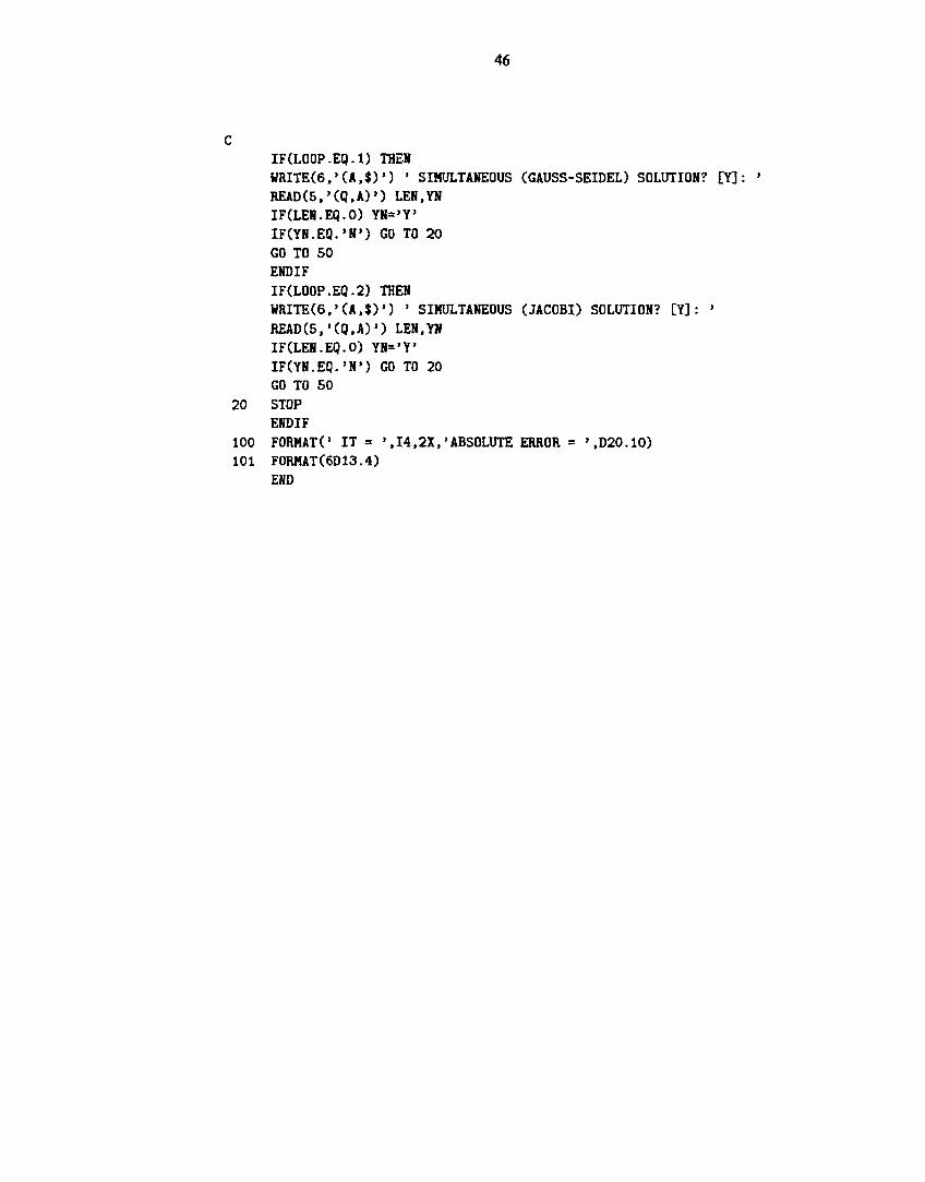
46

IF(LOOP.EQ.l) THEN WRITE(6,'(A,$)') ' SIMULTANEOUS (GAUSS-SEIDEL) SOLUTION? [Y]: » READ(5,'(Q,A)') LEN.YN IF(LEN.EQ.O) YN='Y' IF(YN.EQ.'N') GO TO 20 GO TO 50 ENDIF

IF(L00P.Eq.2) THEN WRrrE(6,'(A.$)') ' SIMULTANEOUS (JACOBI) SOLUTION? [Y]: • READ(5,'(Q,A)') LEN.YN IF(LEN.EQ.O) YN='Y' IFUN.Eq.'N') GO TO 20 GO TO 50

20 STOP ENDIF

100 FORMATC IT = ',14,2X,'ABSOLUTE ERROR - '.D20.10) 101 F0RMAT(6D13.4)

END