1

Lecture 2

Time: M _ _ _ _14:45 - 17:30

MECH 344/X

Machine Element Design

• Introduction to Static Stresses

• Axial, Shear and Torsional Loading

• Bending in Straight and Curved Beams

• Transverse Shear in Beam

• Mohr Circle

• Combined Stresses

• Stress Concentration

• Residual Stresses

Contents of today's lecture

3

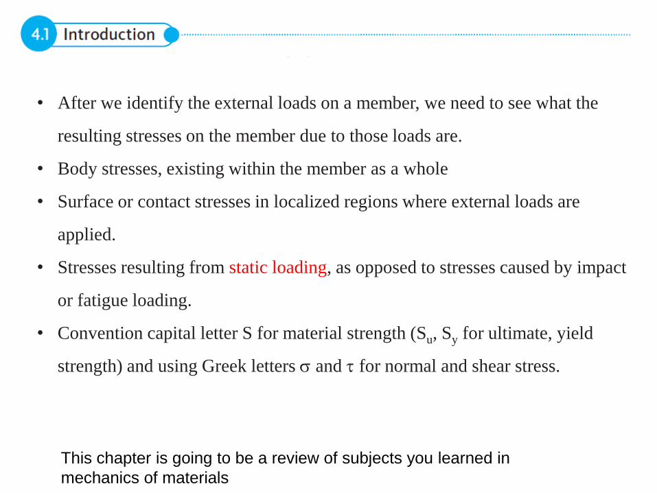
This chapter is going to be a review of subjects you learned in

mechanics of materials

• After we identify the external loads on a member, we need to see what the

resulting stresses on the member due to those loads are.

• Body stresses, existing within the member as a whole

• Surface or contact stresses in localized regions where external loads are

applied.

• Stresses resulting from static loading, as opposed to stresses caused by impact

or fatigue loading.

• Convention capital letter S for material strength (Su, Sy for ultimate, yield

strength) and using Greek letters and for normal and shear stress.

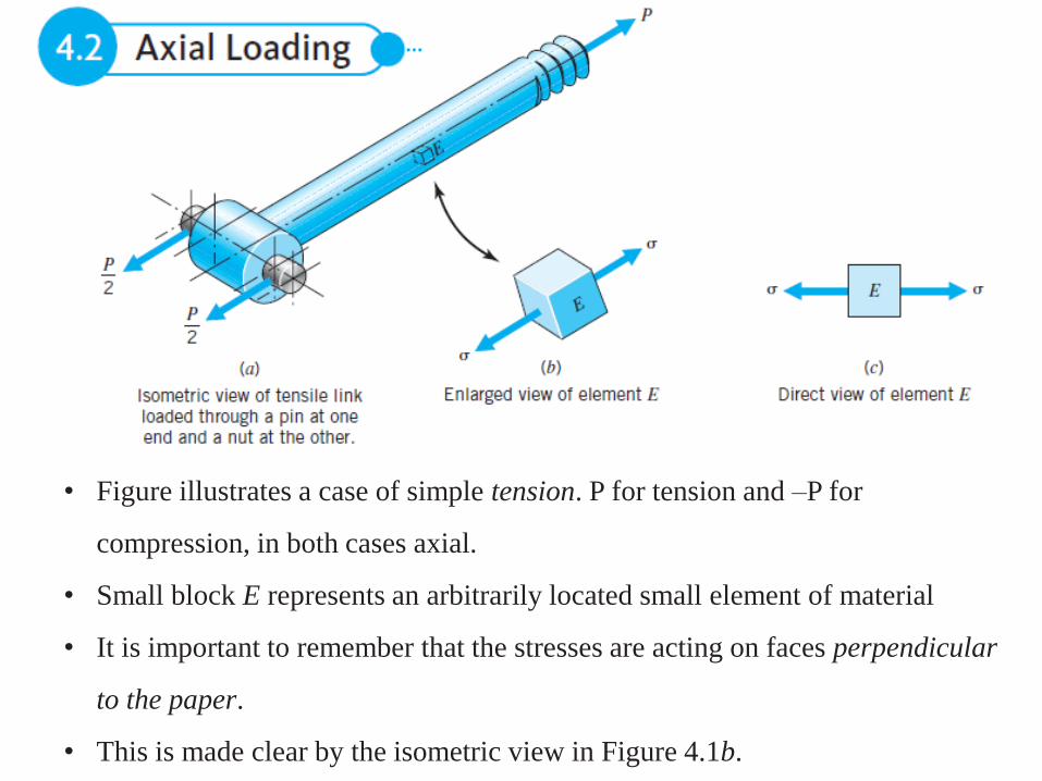
• Figure illustrates a case of simple tension. P for tension and –P for

compression, in both cases axial.

• Small block E represents an arbitrarily located small element of material

• It is important to remember that the stresses are acting on faces perpendicular

to the paper.

• This is made clear by the isometric view in Figure 4.1b.

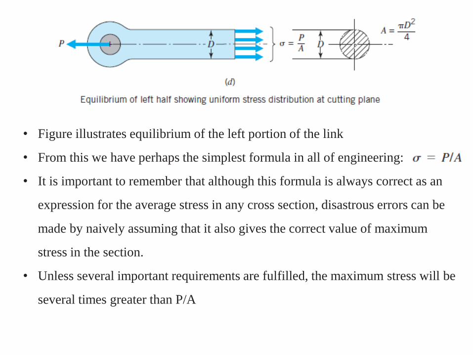
• Figure illustrates equilibrium of the left portion of the link

• From this we have perhaps the simplest formula in all of engineering:

• It is important to remember that although this formula is always correct as an

expression for the average stress in any cross section, disastrous errors can be

made by naively assuming that it also gives the correct value of maximum

stress in the section.

• Unless several important requirements are fulfilled, the maximum stress will be

several times greater than P/A

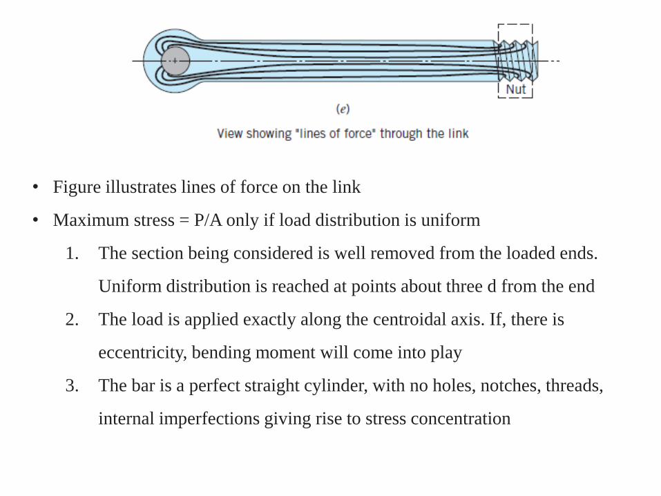
• Figure illustrates lines of force on the link

• Maximum stress = P/A only if load distribution is uniform

1. The section being considered is well removed from the loaded ends.

Uniform distribution is reached at points about three d from the end

2. The load is applied exactly along the centroidal axis. If, there is

eccentricity, bending moment will come into play

3. The bar is a perfect straight cylinder, with no holes, notches, threads,

internal imperfections giving rise to stress concentration

• Figure illustrates lines of force on the link

• Maximum stress = P/A only if load distribution is uniform

4. The bar is free of stress when the external loads are removed. - No

residual stresses due to manufacture and past mechanical/thermal loading

5. The bar comes to stable equilibrium when loaded. If, the bar is in

compression, or if it long, buckling occurs, and elastically unstable.

6. The bar is homogeneous. Not a composite material (where 2 different Es

make a material so that one with larger E gets stressed more)

• 6 welds represent redundant force paths of different stiffnesses.

• The paths to welds 1 and 2 are much stiffer; they may carry nearly all the load.

• A more uniform distribution could be obtained by adding two side plates

• One might despair of ever using P/A as an acceptable value of maximum stress

for relating to the strength properties of the material.

• The student should acquire increasing insight for making “engineering

judgments” relative to these factors as his or her study progresses and

experience grows.

• Figure shows where unexpected

failure can result from assuming

• P is 600 N and 6 identical welds

are used. The average load 100 N

per weld

• If the nut in Figure is tightened to produce an initial bolt tension of P, the direct

shear stresses at the root of the bolt threads (area 2 ), and at the root of the nut

threads (area 3), have average values P/A.

• The thread root areas involved are cylinders of a height equal to the nut

thickness. (for V threads)

• If the shear stress is excessive, shearing or “stripping” of the threads occurs in

the bolt or nut, whichever is weaker.

• Direct shear is used in metal cutting, rivets, pins, keys, splines etc..

• Direct shear loading involves equal and

opposite forces, collinear that the material

between them experiences shear stress,

with negligible bending.

• In figure neglecting interface friction

direct shear with happens @

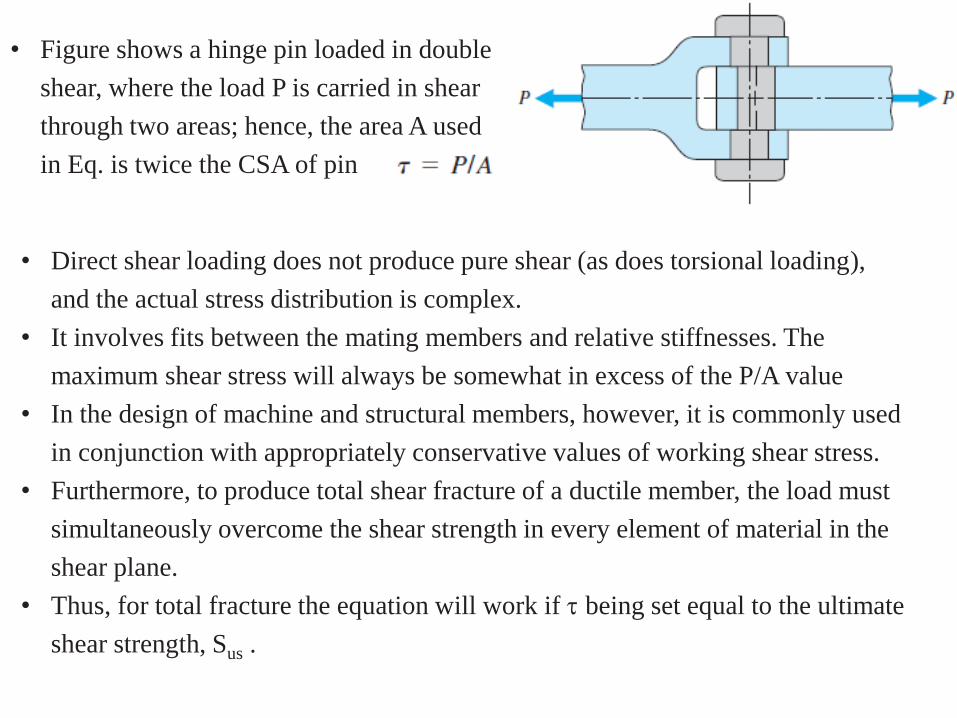
• Direct shear loading does not produce pure shear (as does torsional loading),

and the actual stress distribution is complex.

• It involves fits between the mating members and relative stiffnesses. The

maximum shear stress will always be somewhat in excess of the P/A value

• In the design of machine and structural members, however, it is commonly used

in conjunction with appropriately conservative values of working shear stress.

• Furthermore, to produce total shear fracture of a ductile member, the load must

simultaneously overcome the shear strength in every element of material in the

shear plane.

• Thus, for total fracture the equation will work if being set equal to the ultimate

shear strength, Sus .

• Figure shows a hinge pin loaded in double

shear, where the load P is carried in shear

through two areas; hence, the area A used

in Eq. is twice the CSA of pin

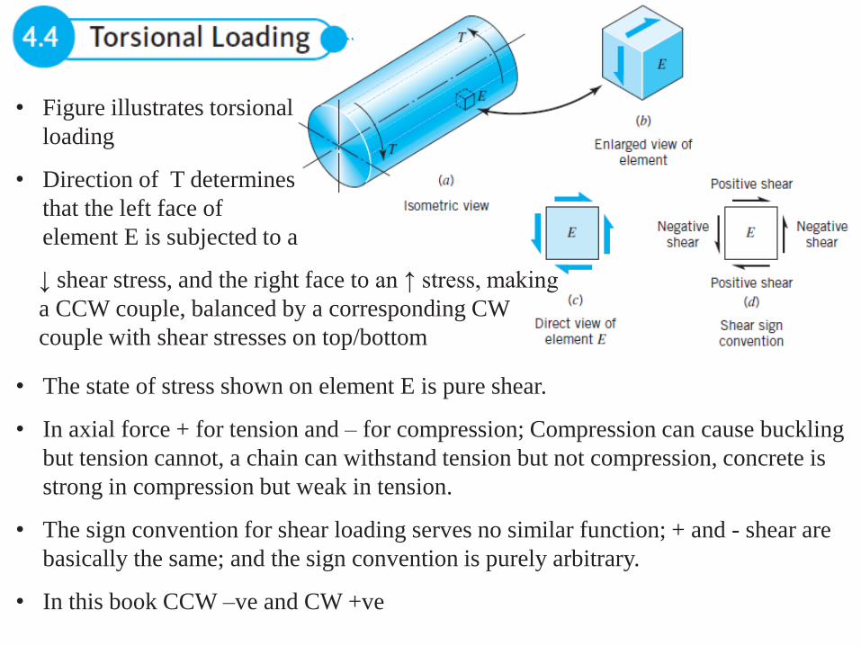
• Figure illustrates torsional

loading

• Direction of T determines

that the left face of

element E is subjected to a

• The state of stress shown on element E is pure shear.

• In axial force + for tension and – for compression; Compression can cause buckling

but tension cannot, a chain can withstand tension but not compression, concrete is

strong in compression but weak in tension.

• The sign convention for shear loading serves no similar function; + and - shear are

basically the same; and the sign convention is purely arbitrary.

• In this book CCW –ve and CW +ve

↓ shear stress, and the right face to an ↑ stress, making

a CCW couple, balanced by a corresponding CW

couple with shear stresses on top/bottom

• For round bar in torsion

stresses vary from 0 at

center to max at surface

• = Tr/J where r is the

radius and J polar moment

• Max shear stress will be

• Important assumptions for this equation are

1. The bar must be straight and round (either solid or hollow), and the torque must

be applied about the longitudinal axis.

2. The material must be homogeneous and perfectly elastic within the stress range

involved.

3. The cross section considered must be sufficiently remote from points of load

application and from stress raisers (i.e., holes, notches, keyways, surface

gouges, etc.).

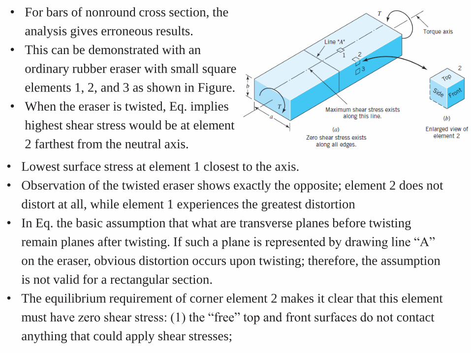
• For bars of nonround cross section, the

analysis gives erroneous results.

• This can be demonstrated with an

ordinary rubber eraser with small square

elements 1, 2, and 3 as shown in Figure.

• When the eraser is twisted, Eq. implies

highest shear stress would be at element

2 farthest from the neutral axis.

• Lowest surface stress at element 1 closest to the axis.

• Observation of the twisted eraser shows exactly the opposite; element 2 does not

distort at all, while element 1 experiences the greatest distortion

• In Eq. the basic assumption that what are transverse planes before twisting

remain planes after twisting. If such a plane is represented by drawing line “A”

on the eraser, obvious distortion occurs upon twisting; therefore, the assumption

is not valid for a rectangular section.

• The equilibrium requirement of corner element 2 makes it clear that this element

must have zero shear stress: (1) the “free” top and front surfaces do not contact

anything that could apply shear stresses;

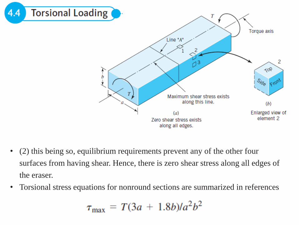
• (2) this being so, equilibrium requirements prevent any of the other four

surfaces from having shear. Hence, there is zero shear stress along all edges of

the eraser.

• Torsional stress equations for nonround sections are summarized in references

15

• Pure Bending – it is rare for beam to be loaded in pure

bending. It is useful though to understand the situation

• Mostly shear loading and bending moments act

together

• Applying point loads P equidistant at the simply

supported beam, absence of shear loading makes this

pure bending

• Assumptions used for analysis

16

17

• N-N along the neutral axis, no change in length

• A-A shortents (in compression) and B-B lengthens (in tension

• Bending stress is 0 at N-N and is linearly proportional to distance y away from

N-N

• Where M is the bending moment and I is the area moment of Inertia of

the beam cross section at the neutral plane, y the distance from N-N

• The max stress at outer plane is

• Where c is distance from neutral plane (it should be same both sections

if the beam is symmetrical about the neutral axis

• C is taken as +ve

initially and

proper sign

applied based on

loading

compression –ve

and tension +ve

• Figure shows bending load applied to beam of CS having 2 axes of symmetry

• cutting-plane stresses max are obtained from Eq. 4.6 by substituting c for y

• Section modulus Z (I/c) is used, giving max as

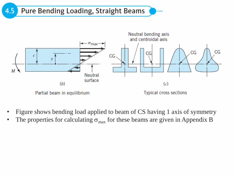
• Figure shows bending load applied to beam of CS having 1 axis of symmetry

• The properties for calculating max for these beams are given in Appendix B

20

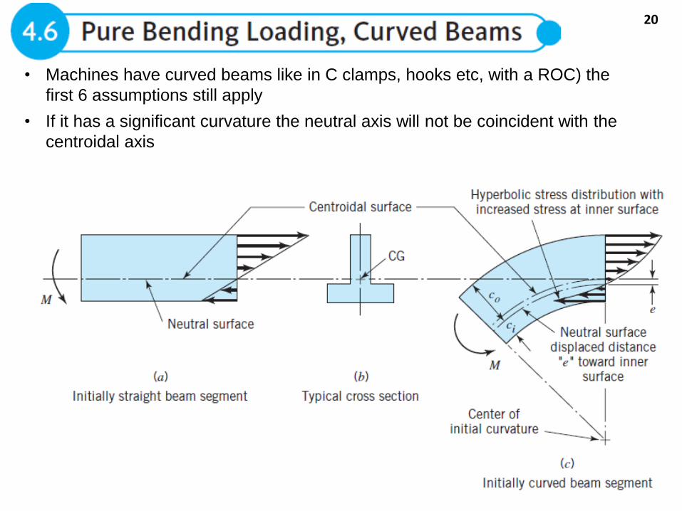
• Machines have curved beams like in C clamps, hooks etc, with a ROC) the

first 6 assumptions still apply

• If it has a significant curvature the neutral axis will not be coincident with the

centroidal axis

21

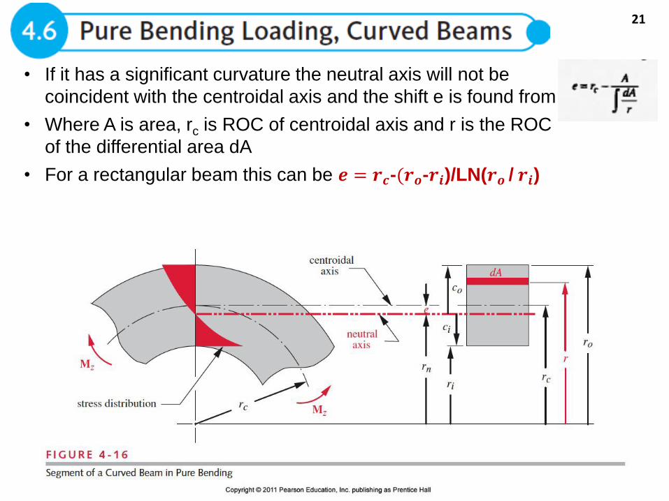
• If it has a significant curvature the neutral axis will not be

coincident with the centroidal axis and the shift e is found from

• Where A is area, rc is ROC of centroidal axis and r is the ROC

of the differential area dA

• For a rectangular beam this can be 𝒆 = 𝒓𝒄-(𝒓𝒐-𝒓𝒊)/LN(𝒓𝒐 / 𝒓𝒊)

22

• Stress distribution is not linear but hyperbolic. Sign convention is +ve moment

straightens the beam (tension inside and compression outside)

• For pure bending loads stresses at inner and outer surface is

• And if a force F on the CSA “A” is applied on the curved beam

then the stresses will be

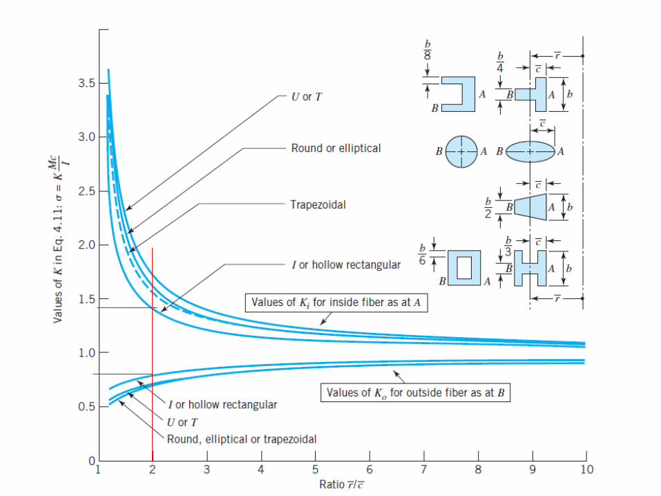
Stress values given by Eq differ from the straight-beam “Mc/I”

value by a curvature factor, K. Thus, using subscripts i and o to

denote inside and outside fibers, respectively, we have

Values of K in Figure illustrates a common rule of thumb: “If r is

at least ten times inner fiber stresses are usually not more

than 10 percent above the Mc/I value.” Values of Ko, Ki , and e

are tabulated for several cross sections in references.

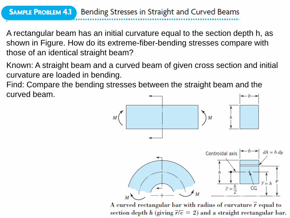
A rectangular beam has an initial curvature equal to the section depth h, as

shown in Figure. How do its extreme-fiber-bending stresses compare with

those of an identical straight beam?

Known: A straight beam and a curved beam of given cross section and initial

curvature are loaded in bending.

Find: Compare the bending stresses between the straight beam and the

curved beam.

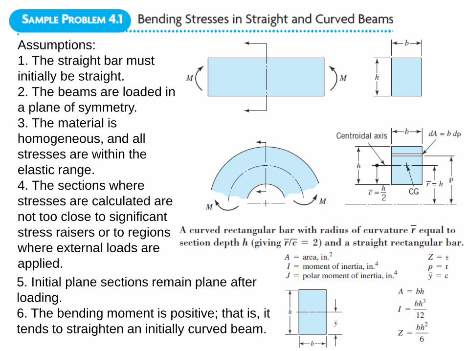
Assumptions:

1. The straight bar must

initially be straight.

2. The beams are loaded in

a plane of symmetry.

3. The material is

homogeneous, and all

stresses are within the

elastic range.

4. The sections where

stresses are calculated are

not too close to significant

stress raisers or to regions

where external loads are

applied.

5. Initial plane sections remain plane after

loading.

6. The bending moment is positive; that is, it

tends to straighten an initially curved beam.

• e = rc-(ro-ri)/LN(ro / ri)

• ro = 1.5h and ri = .5h and rc = h

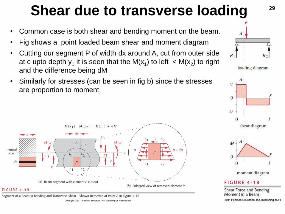
29Shear due to transverse loading

• Common case is both shear and bending moment on the beam.

• Fig shows a point loaded beam shear and moment diagram

• Cutting our segment P of width dx around A, cut from outer side

at c upto depth y1 it is seen that the M(x1) to left < M(x2) to right

and the difference being dM

• Similarly for stresses (can be seen in fig b) since the stresses

are proportion to moment

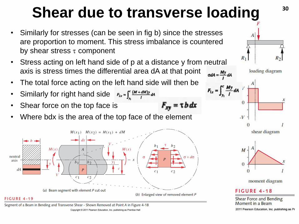
30Shear due to transverse loading

• Similarly for stresses (can be seen in fig b) since the stresses

are proportion to moment. This stress imbalance is countered

by shear stress component

• Stress acting on left hand side of p at a distance y from neutral

axis is stress times the differential area dA at that point

• The total force acting on the left hand side will then be

• Similarly for right hand side

• Shear force on the top face is

• Where bdx is the area of the top face of the element

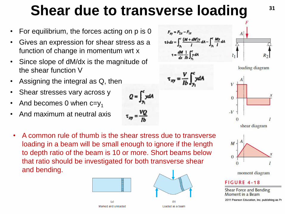
31Shear due to transverse loading

• For equilibrium, the forces acting on p is 0

• Gives an expression for shear stress as a

function of change in momentum wrt x

• Since slope of dM/dx is the magnitude of

the shear function V

• Assigning the integral as Q, then

• Shear stresses vary across y

• And becomes 0 when c=y1

• And maximum at neutral axis

• A common rule of thumb is the shear stress due to transverse

loading in a beam will be small enough to ignore if the length

to depth ratio of the beam is 10 or more. Short beams below

that ratio should be investigated for both transverse shear

and bending.

32

33

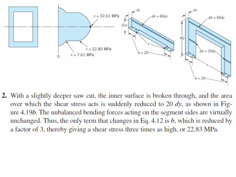
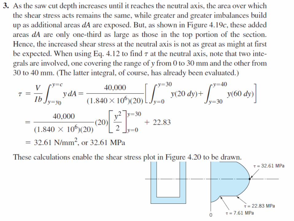
Determine the shear stress distribution for the beam and loading

shown in Figure 4.18. Compare this with the maximum bending

stress.

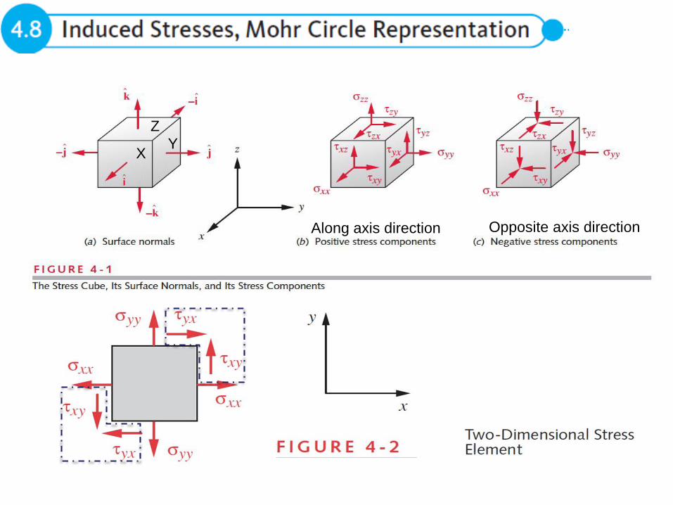
Along axis direction Opposite axis direction

XY

Z

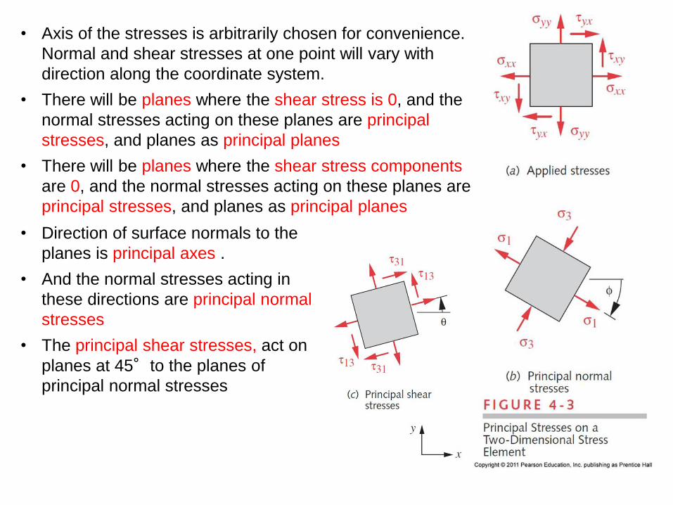
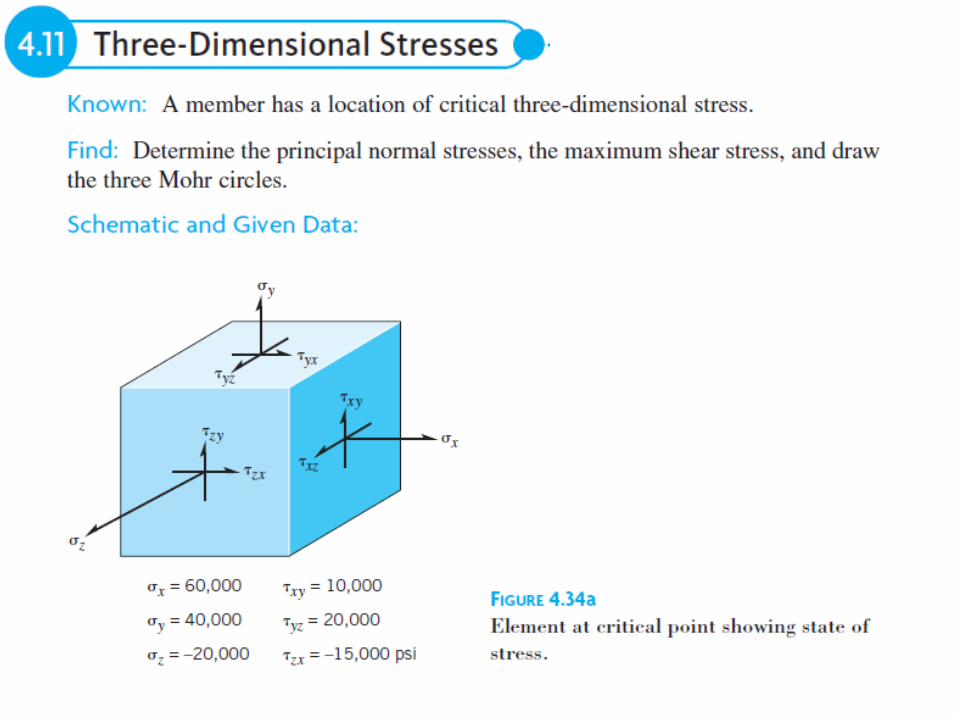
41• Axis of the stresses is arbitrarily chosen for convenience.

Normal and shear stresses at one point will vary with

direction along the coordinate system.

• There will be planes where the shear stress is 0, and the

normal stresses acting on these planes are principal

stresses, and planes as principal planes

• There will be planes where the shear stress components

are 0, and the normal stresses acting on these planes are

principal stresses, and planes as principal planes

• Direction of surface normals to the

planes is principal axes .

• And the normal stresses acting in

these directions are principal normal

stresses

• The principal shear stresses, act on

planes at 45°to the planes of

principal normal stresses

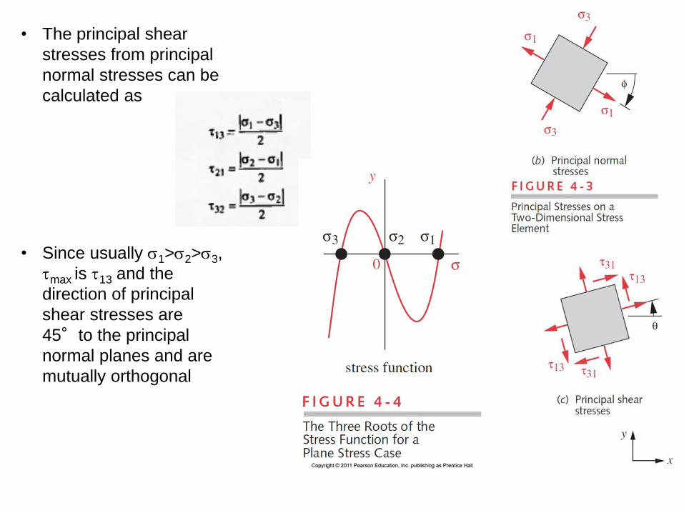
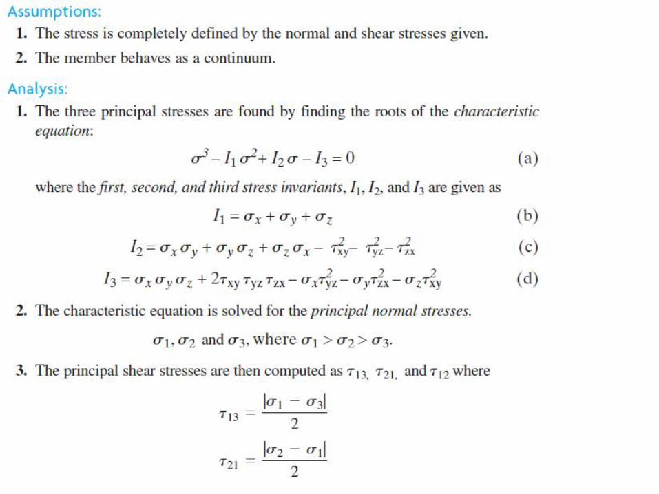
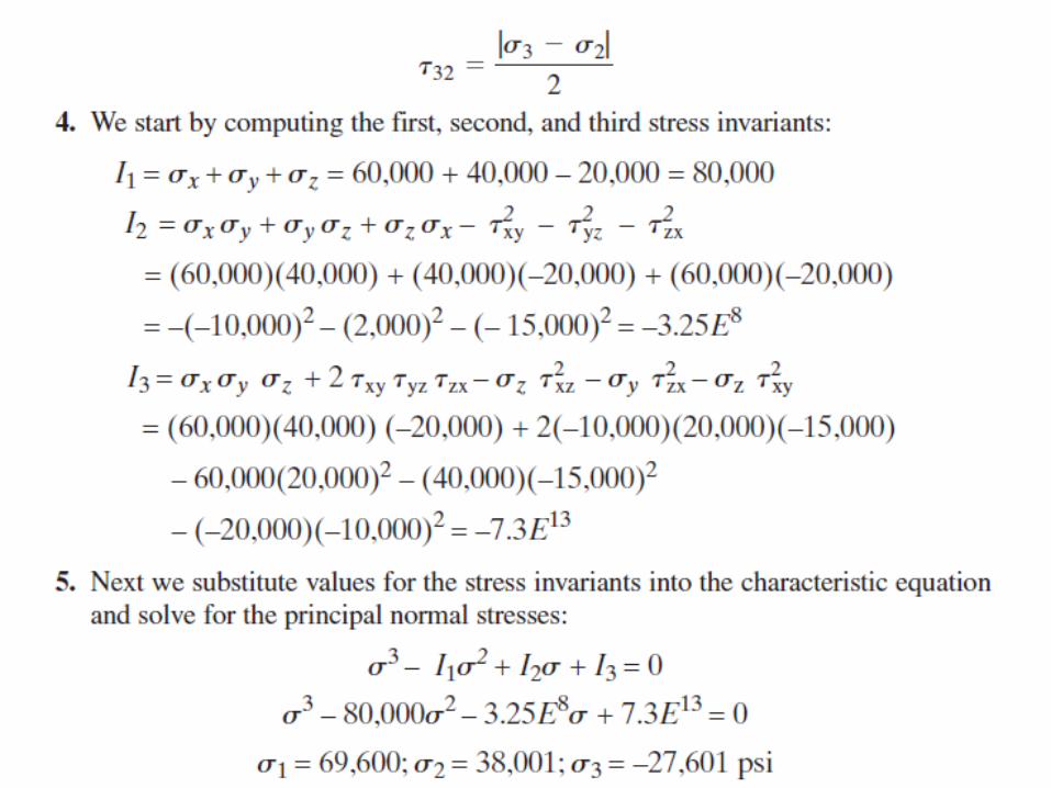
43• The principal shear

stresses from principal

normal stresses can be

calculated as

• Since usually 1>2>3,

max is 13 and the

direction of principal

shear stresses are

45°to the principal

normal planes and are

mutually orthogonal

44

• Mohr circle is a graphical method find the principal stresses

The Mohr’s Circle

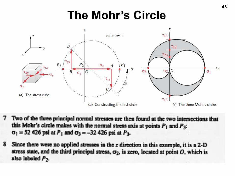
45

The Mohr’s Circle

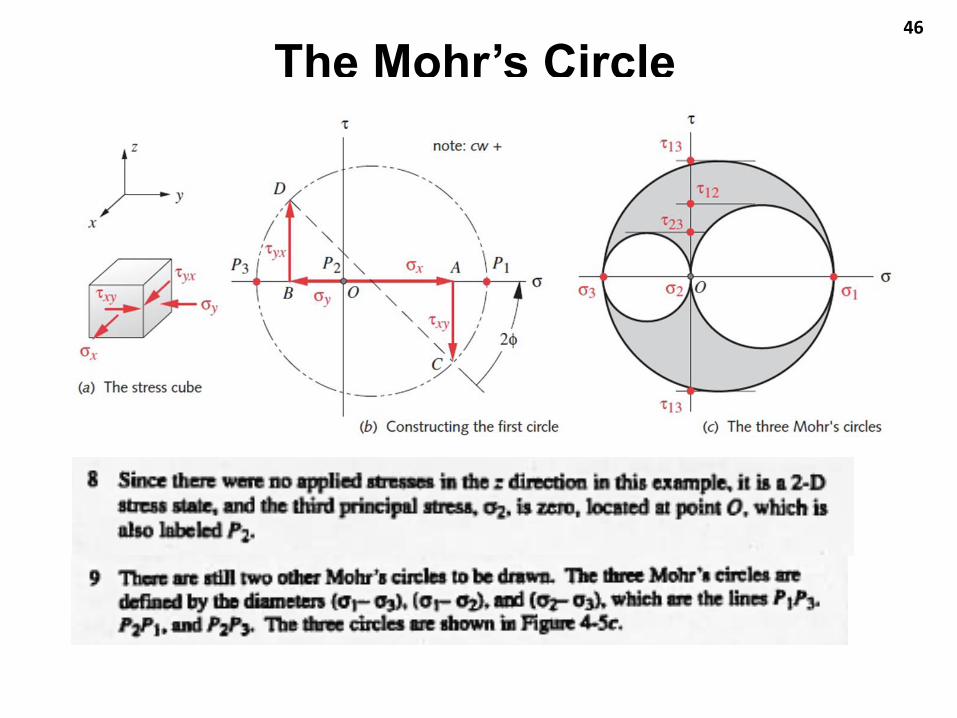
46

The Mohr’s Circle

47

The Mohr’s Circle

48

49

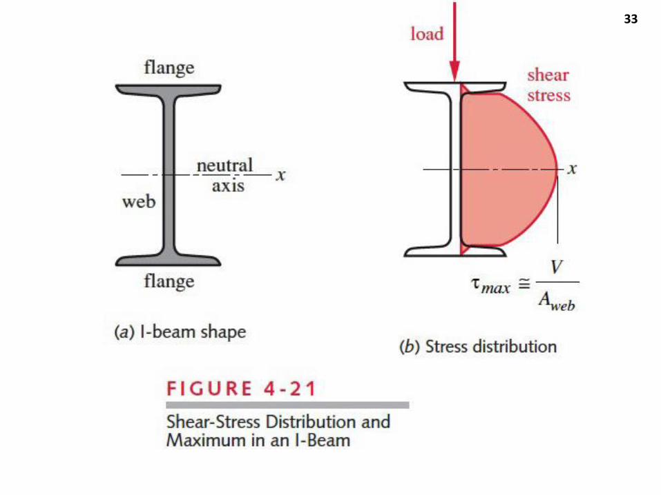
• The shaft is subjected to torsion, bending, and transverse shear. Torsional stresses

are max @ shaft surface. Bending stresses are a maximum at points A and B

• Transverse shear stresses are relatively small compared to bending stresses, and

equal to zero at points A and B

50

• Since the largest of the three

Mohr circles always represents

the maximum shear stress as

well as the two extreme values of

normal stress, Mohr called this

the principal circle.

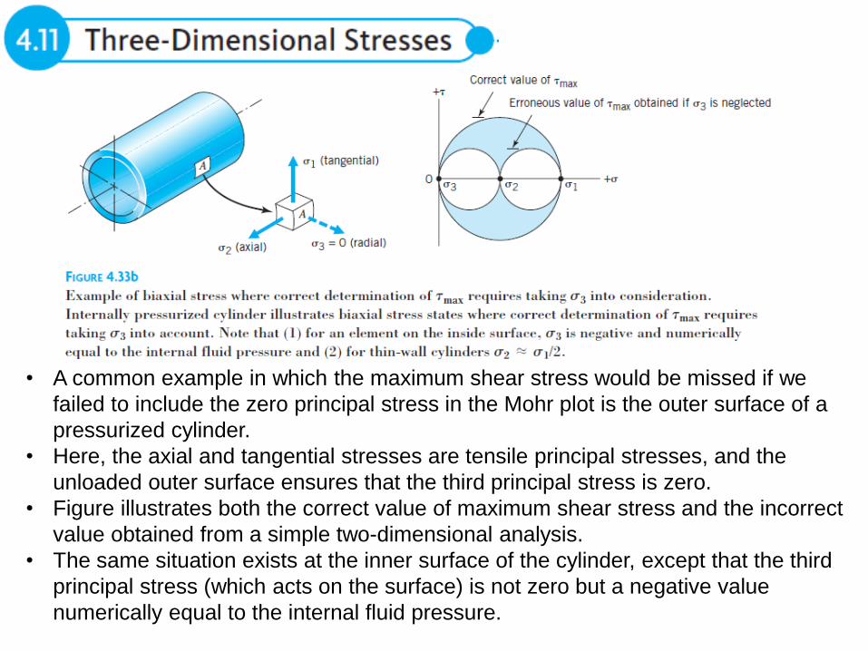
• A common example in which the maximum shear stress would be missed if we

failed to include the zero principal stress in the Mohr plot is the outer surface of a

pressurized cylinder.

• Here, the axial and tangential stresses are tensile principal stresses, and the

unloaded outer surface ensures that the third principal stress is zero.

• Figure illustrates both the correct value of maximum shear stress and the incorrect

value obtained from a simple two-dimensional analysis.

• The same situation exists at the inner surface of the cylinder, except that the third

principal stress (which acts on the surface) is not zero but a negative value

numerically equal to the internal fluid pressure.

• Figure indicates lines of force flow through a tensile link.

• Uniform distribution of these lines exist in regions away from the ends.

• At the ends, the force flow lines indicate stress concentration near outer surface.

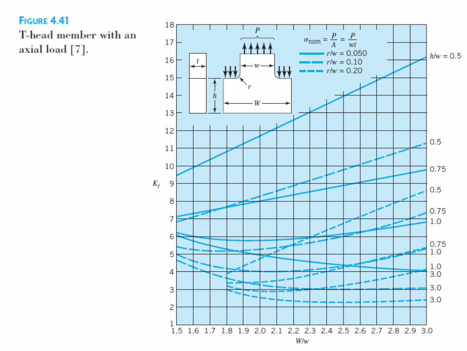
• We need to evaluate the stress concentration associated with various geometric

configurations to determine maximum stresses existing in a part

• The first mathematical treatments of stress concentration were published after

1900 with experimental methods for measuring highly localized stresses

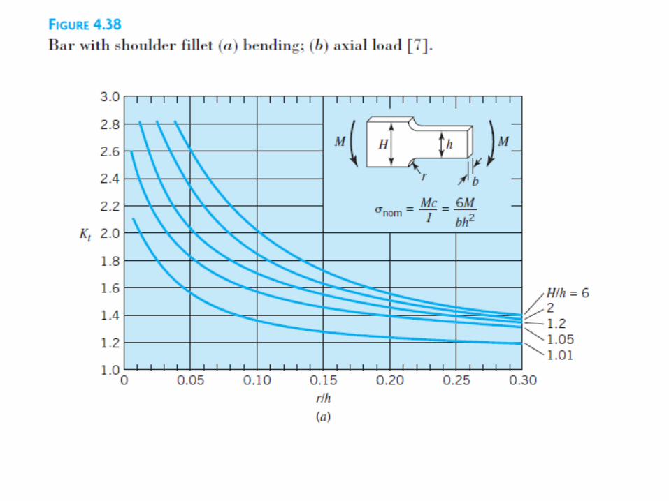
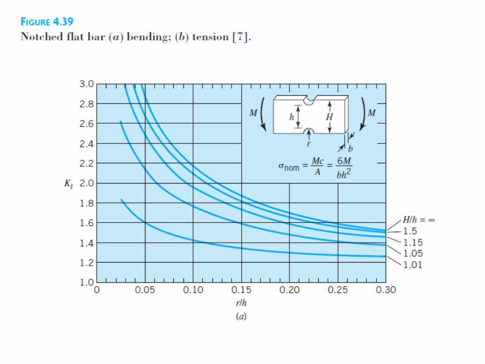
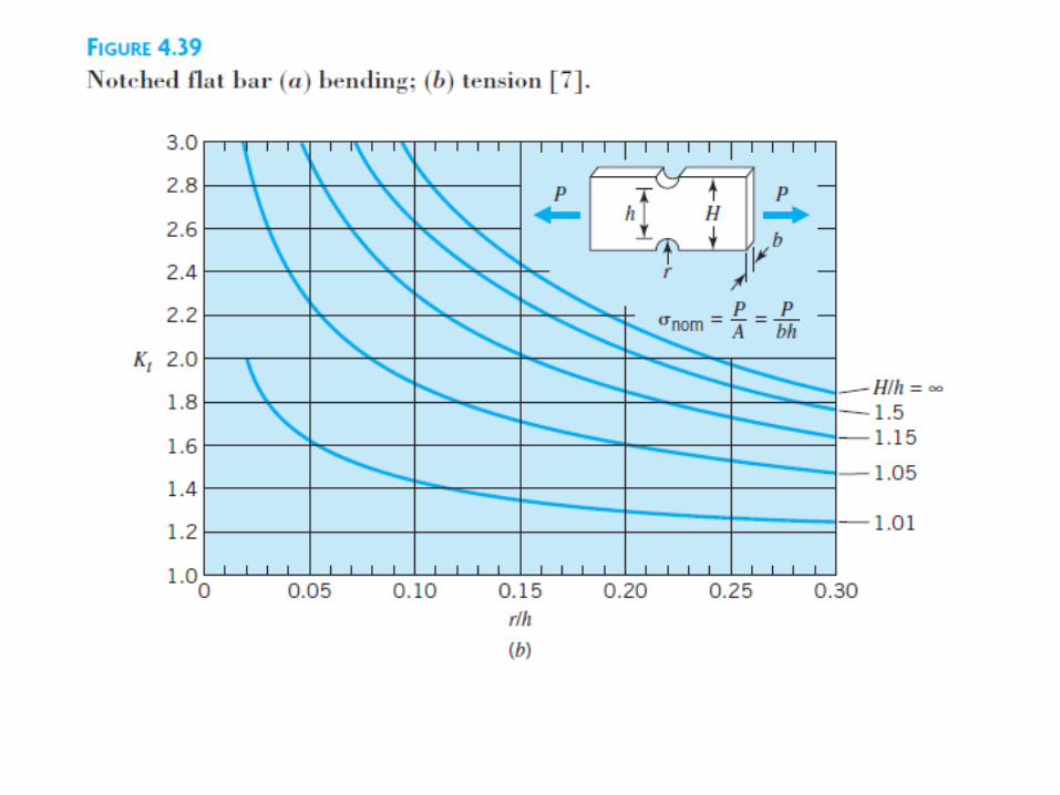
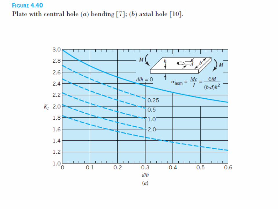
• In recent years, FEM studies have also been employed. The results of many of

these studies are available in the form of published graphs giving values of the

theoretical stress concentration factor, Kt (based on a theoretical elastic,

homogeneous, isotropic material), for use in the equations

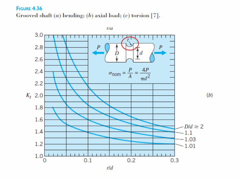
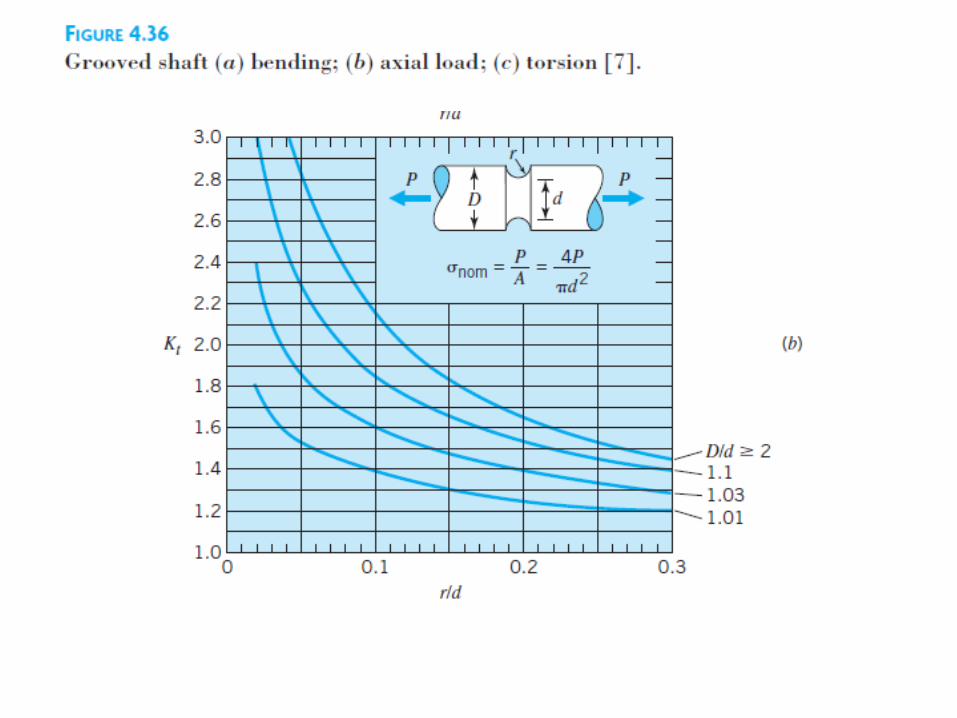
• For eg, the maximum stress for axial loading would be P/A * appropriate Kt .

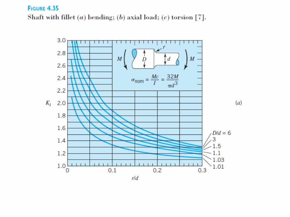
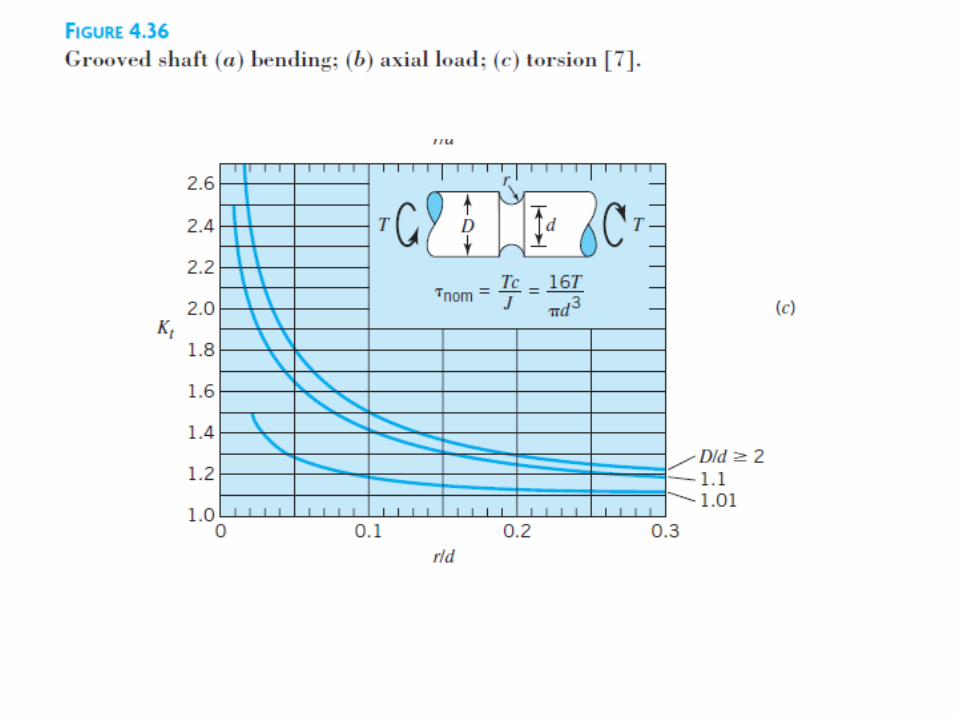
• Note that the stress concentration graphs are plotted on the basis of dimensionless

ratios, indicating that only part shape (not size) is involved. Also note that stress

concentration factors are different for axial, bending, and torsional loading.

• In many situations involving notched parts in tension or bending, the notch not only

increases the primary stress but also causes one or both of the other principal

stresses to take on nonzero values.

• This is referred to as the biaxial or triaxial effect of stress raisers (“stress raiser” is a

general term applied to notches, holes, threads, etc.).

• Consider, for example, a soft rubber model of the grooved shaft in tension illustrated

in Figure 4.36b. As the tensile load is increased, there will be a tendency for the

outer surface to pull into a smooth cylinder.

• This will involve an increase in the diameter and circumference of the section in the

plane of the notch. The increased circumference gives rise to a tangential stress,

which is a maximum at the surface. The increase in diameter is associated with the

creation of radial stresses. (Remember, though, that this radial stress must be zero

at the surface because there are no external radial forces acting there.)

• Kt factors given in the graphs are theoretical (hence, the subscript t) or

geometric factors based on a theoretical homogeneous, isotropic, & elastic mat’l

• Real materials have microscopic irregularities causing a certain nonuniformity of

microscopic stress distribution, even in notch-free parts.

• Hence, the introduction of a stress raiser may not cause as much additional

damage as indicated by the theoretical factor.

• Moreover, real parts—even if free of stress raisers—have surface irregularities

(from processing and use) that can be considered as extremely small notches.

• The extent to which we must take stress concentration into account depends on

• (1) the extent to which the real material deviates from the theoretical and

• (2) whether the loading is static, or fatigue

• For materials permeated with internal discontinuities, such as gray cast iron,

stress raisers usually have little effect, regardless of the nature of loading, as

geometric irregularities affect less than the internal irregularities.

• For fatigue & impact loading of engineering materials, Kt must be considered

• For the case of static loading, Kt is important only with unusual materials that

are both brittle and relatively homogeneous;

• When tearing a package wrapped in clear plastic film, a sharp notch in the

edge is most helpful!

• or for normally ductile materials that, under special conditions, behave in a

brittle manner

• For the usual engineering materials having some ductility (and under conditions

such that they behave as ductile), it is customary to ignore Kt for static loads.

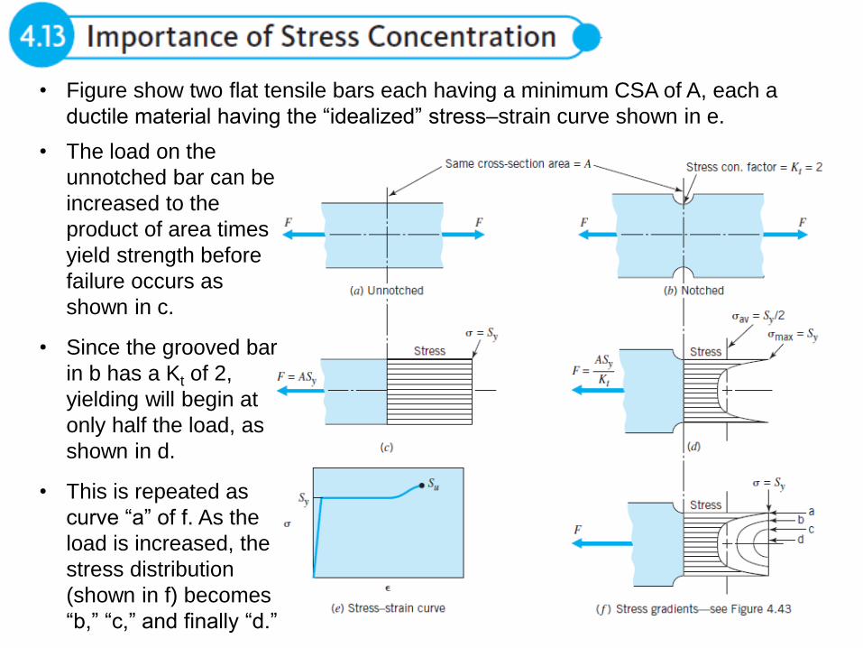
• Figure show two flat tensile bars each having a minimum CSA of A, each a

ductile material having the “idealized” stress–strain curve shown in e.

• The load on the

unnotched bar can be

increased to the

product of area times

yield strength before

failure occurs as

shown in c.

• Since the grooved bar

in b has a Kt of 2,

yielding will begin at

only half the load, as

shown in d.

• This is repeated as

curve “a” of f. As the

load is increased, the

stress distribution

(shown in f) becomes

“b,” “c,” and finally “d.”

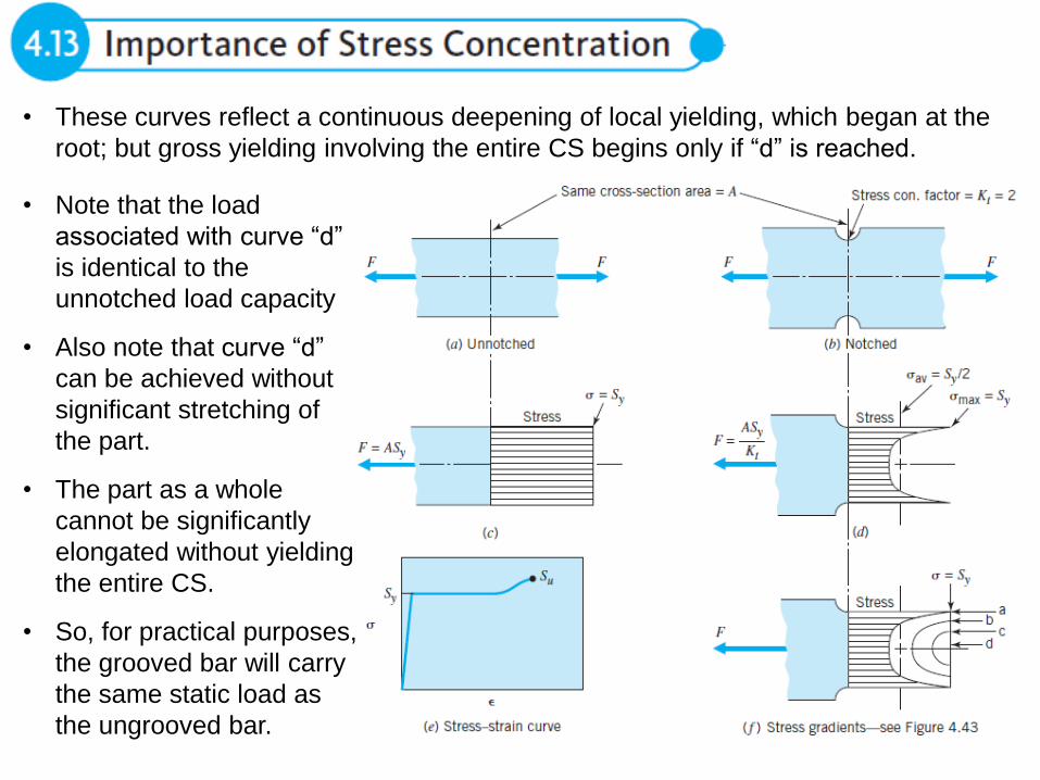
• These curves reflect a continuous deepening of local yielding, which began at the

root; but gross yielding involving the entire CS begins only if “d” is reached.

• Note that the load

associated with curve “d”

is identical to the

unnotched load capacity

• Also note that curve “d”

can be achieved without

significant stretching of

the part.

• The part as a whole

cannot be significantly

elongated without yielding

the entire CS.

• So, for practical purposes,

the grooved bar will carry

the same static load as

the ungrooved bar.

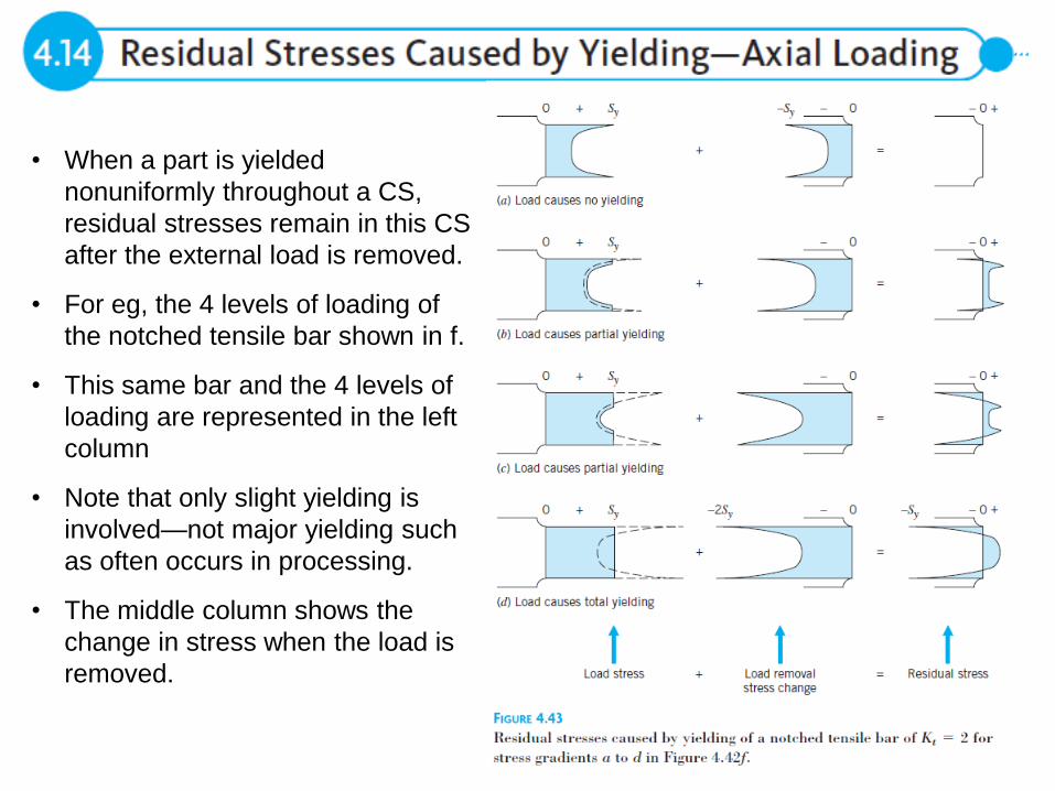
• When a part is yielded

nonuniformly throughout a CS,

residual stresses remain in this CS

after the external load is removed.

• For eg, the 4 levels of loading of

the notched tensile bar shown in f.

• This same bar and the 4 levels of

loading are represented in the left

column

• Note that only slight yielding is

involved—not major yielding such

as often occurs in processing.

• The middle column shows the

change in stress when the load is

removed.

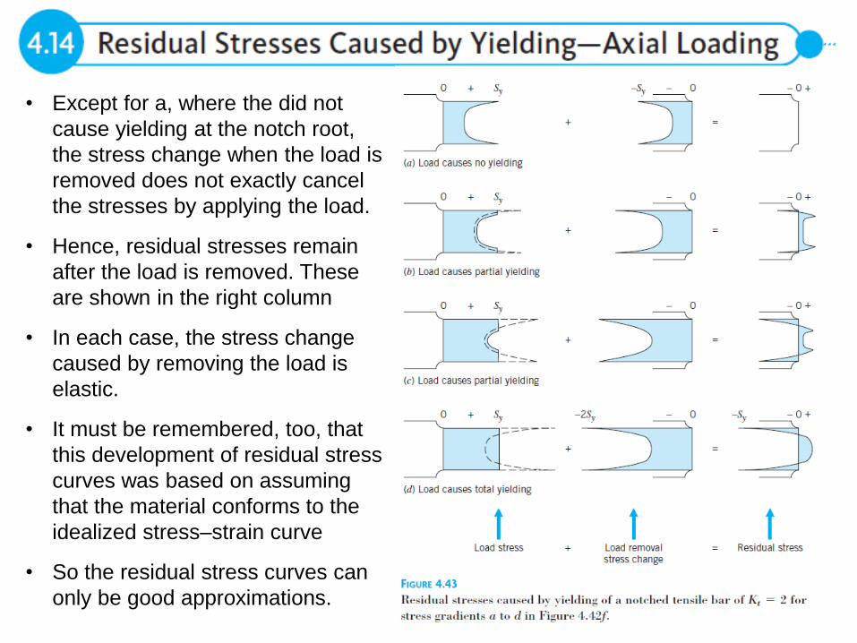
• Except for a, where the did not

cause yielding at the notch root,

the stress change when the load is

removed does not exactly cancel

the stresses by applying the load.

• Hence, residual stresses remain

after the load is removed. These

are shown in the right column

• In each case, the stress change

caused by removing the load is

elastic.

• It must be remembered, too, that

this development of residual stress

curves was based on assuming

that the material conforms to the

idealized stress–strain curve

• So the residual stress curves can

only be good approximations.

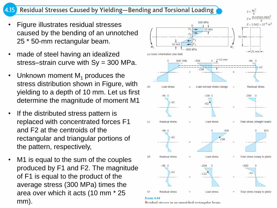
• Figure illustrates residual stresses

caused by the bending of an unnotched

25 * 50-mm rectangular beam.

• made of steel having an idealized

stress–strain curve with Sy = 300 MPa.

• Unknown moment M1 produces the

stress distribution shown in Figure, with

yielding to a depth of 10 mm. Let us first

determine the magnitude of moment M1

• If the distributed stress pattern is

replaced with concentrated forces F1

and F2 at the centroids of the

rectangular and triangular portions of

the pattern, respectively,

• M1 is equal to the sum of the couples

produced by F1 and F2. The magnitude

of F1 is equal to the product of the

average stress (300 MPa) times the

area over which it acts (10 mm * 25

mm).

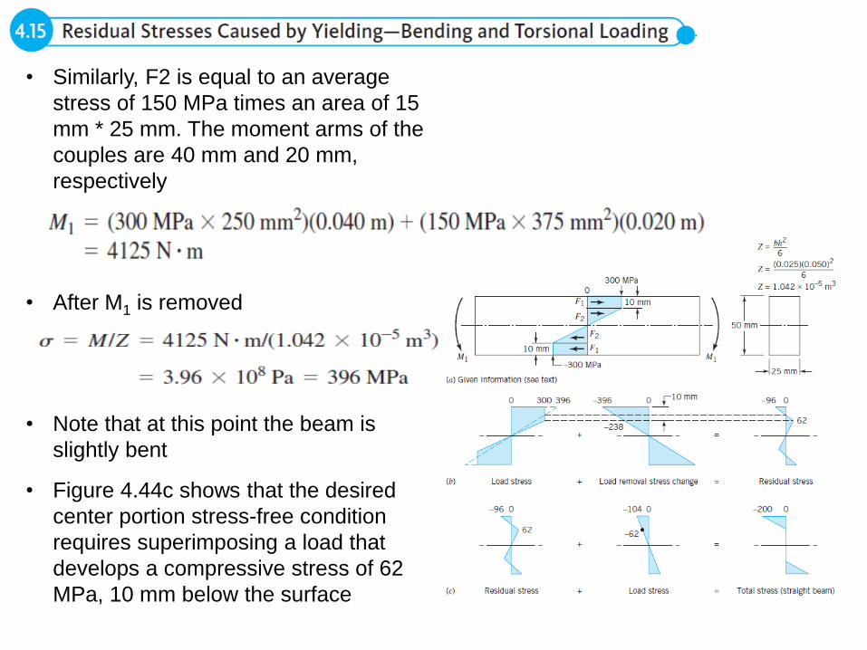
• Similarly, F2 is equal to an average

stress of 150 MPa times an area of 15

mm * 25 mm. The moment arms of the

couples are 40 mm and 20 mm,

respectively

• After M1 is removed

• Note that at this point the beam is

slightly bent

• Figure 4.44c shows that the desired

center portion stress-free condition

requires superimposing a load that

develops a compressive stress of 62

MPa, 10 mm below the surface

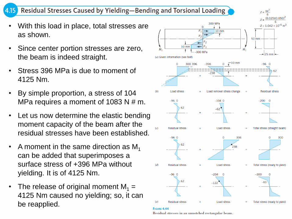
• With this load in place, total stresses are

as shown.

• Since center portion stresses are zero,

the beam is indeed straight.

• Stress 396 MPa is due to moment of

4125 Nm.

• By simple proportion, a stress of 104

MPa requires a moment of 1083 N # m.

• Let us now determine the elastic bending

moment capacity of the beam after the

residual stresses have been established.

• A moment in the same direction as M1

can be added that superimposes a

surface stress of +396 MPa without

yielding. It is of 4125 Nm.

• The release of original moment M1 =

4125 Nm caused no yielding; so, it can

be reapplied.

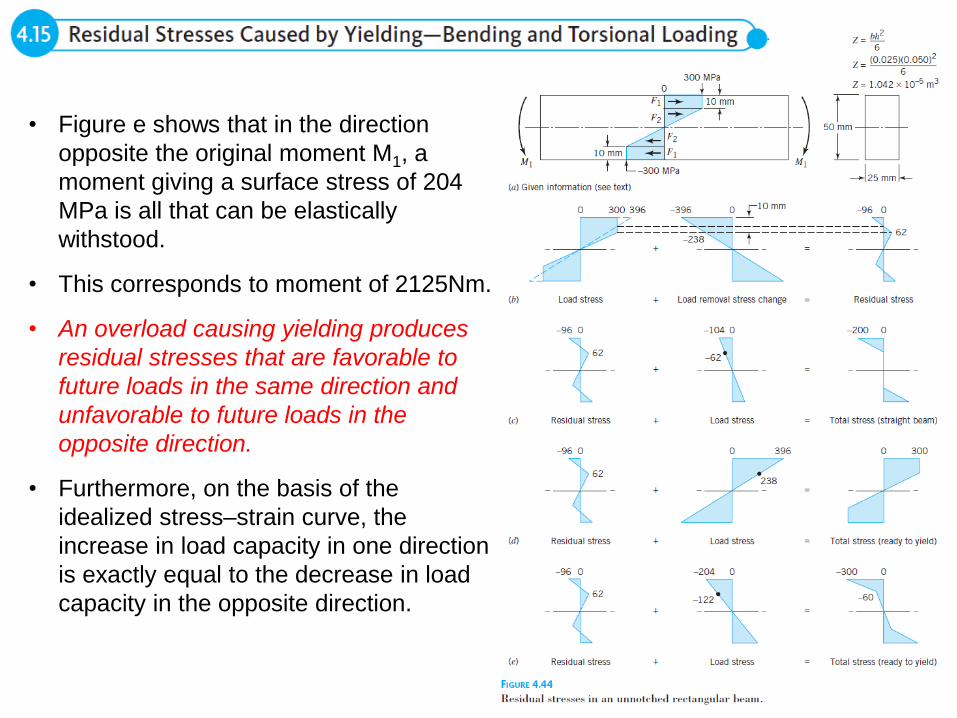
• Figure e shows that in the direction

opposite the original moment M1, a

moment giving a surface stress of 204

MPa is all that can be elastically

withstood.

• This corresponds to moment of 2125Nm.

• An overload causing yielding produces

residual stresses that are favorable to

future loads in the same direction and

unfavorable to future loads in the

opposite direction.

• Furthermore, on the basis of the

idealized stress–strain curve, the

increase in load capacity in one direction

is exactly equal to the decrease in load

capacity in the opposite direction.

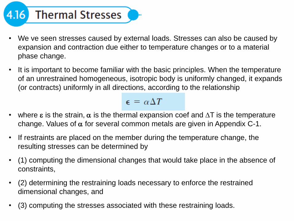
• We ve seen stresses caused by external loads. Stresses can also be caused by

expansion and contraction due either to temperature changes or to a material

phase change.

• It is important to become familiar with the basic principles. When the temperature

of an unrestrained homogeneous, isotropic body is uniformly changed, it expands

(or contracts) uniformly in all directions, according to the relationship

• where is the strain, is the thermal expansion coef and T is the temperature

change. Values of for several common metals are given in Appendix C-1.

• If restraints are placed on the member during the temperature change, the

resulting stresses can be determined by

• (1) computing the dimensional changes that would take place in the absence of

constraints,

• (2) determining the restraining loads necessary to enforce the restrained

dimensional changes, and

• (3) computing the stresses associated with these restraining loads.

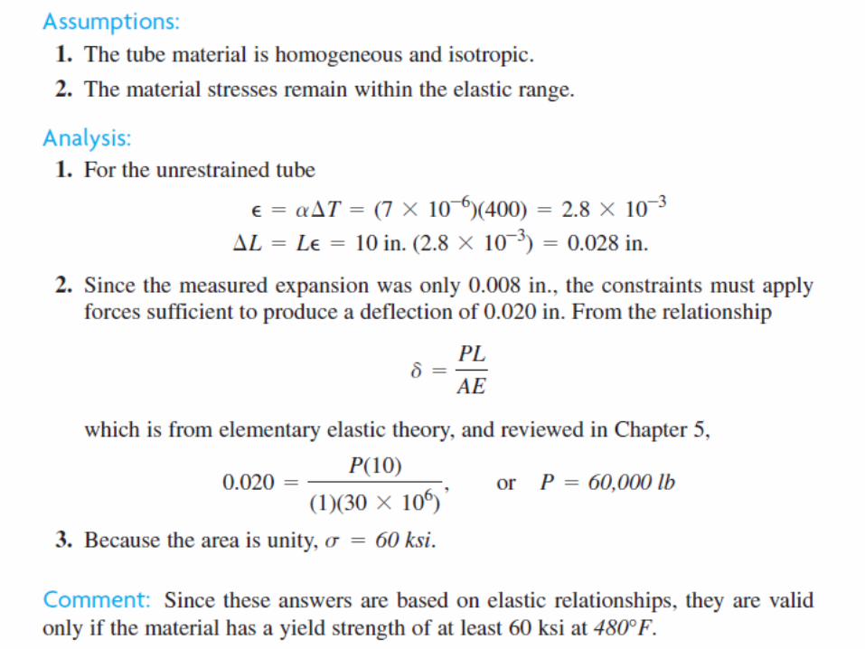
• We ve seen stresses caused by external loads. Stresses can also be caused by

expansion and contraction due either to temperature changes or to a material

phase change. A 10-in. L steel tube (E = 30 X 106 psi and = 7 X 10-6 per °F)

having a CSA of 1 in2 is installed with “fixed” ends so that it is stress-free at

80°F. In operation, the tube is heated throughout to a uniform 480°F. Careful

measurements indicate that the fixed ends separate by 0.008 in. What loads are

exerted on the ends of the tube, and what are the resultant stresses?

• Known: A

given length of

steel tubing

with a known

CSA expands

0.008 in. from

a stress-free

condition at

80°F when

the tube is

heated to a

uniform

480°F

• If stresses caused by temperature change are undesirably large, the best

solution is often to reduce the constraint. - using expansion joints, loops,

or telescopic joints

• Thermal stresses also result due to temperature gradients - if a thick metal

plate is heated in the center of one face with a torch, the hot surface is

restrained from expanding by the cooler surrounding material; it is in a

state of compression.

• Then the remote cooler metal is forced to expand, causing tensile

stresses.

• If the forces and moments do not balance for the original geometry, it will

distort or warp to bring about internal equilibrium.

• If stresses are within the elastic limit, the part will revert to its original

geometry when the initial temperature conditions are restored.

• If some portion of the part yields, this portion will not tend to revert to the

initial geometry, and there will be warpage and internal (residual) stresses

when initial temperature conditions are restored. This must be taken into

account in the design

• Residual stresses are added to any subsequent load stresses in order to

obtain the total stresses.

• If a part with residual stresses is machined, the removal of residually

stressed material causes the part to warp or distort. As this upsets the

internal equilibrium.

• A common (destructive) method for determining the residual stress in a

particular zone of a part is to remove very carefully material from the zone

and then to make a precision measurement of the resulting change in

geometry. (Hole drilling method)

• Residual stresses are often removed by annealing. The unrestrained part

is uniformly heated (to a sufficiently high temperature and for a sufficiently

long period of time) to cause virtually complete relief of the internal

stresses by localized yielding.

• The subsequent slow cooling operation introduces no yielding. Hence, the

part reaches room temperature in a virtually stress-free state.

• In general, residual stresses are important in situations in which stress

concentration is important.

• These include brittle materials involving all loading types, and the fatigue and

impact loading of ductile as well as brittle materials.

• For the static loading of ductile materials, harmless local yielding can usually

occur to relieve local high stresses resulting from either (or both) stress

concentration or superimposed residual stress.

• It is easy to overlook residual stresses because they involve nothing that ordinarily

brings them to the attention of the senses. When one holds an unloaded machine

part, for example, there is normally no way of knowing whether the stresses are

all zero or whether large residual stresses are present.

• a reasonable qualitative estimate can often be made by considering the thermal

and mechanical loading history of the part.

• An interesting example shows that residual stresses remain in a part as long as

heat or external loading does not remove them by yielding.

• The Liberty Bell, cast in 1753, has

residual tensile stresses in the

outer surface because the casting

cooled most rapidly from the inside

surface.

• After 75 years of satisfactory

service, the bell cracked, probably

as a result of fatigue from

superimposed vibratory stresses

caused by ringing the bell.

• Holes were drilled at the ends to

keep the crack from growing, but

the crack subsequently extended

itself.

• Almen and Black cite this as proof

that residual stresses are still

present in the bell.